Embed Size (px)
Citation preview

2015
MMFI THESIS Wits Business School University of the Witwatersrand Johannesburg, South Africa Supervisor: Prof Kalu Ojah
Hugh Napier 9601398N
[AN EMPIRICAL ANALYSIS OF
MACROECONOMIC FACTORS AND THE EFFECTS ON INSURANCE DEMAND AND
PROFITABILITY] .

ii | P a g e
Acknowledgements
Only occasionally do functional requirements overlap with ones interests. It has been as much a
pleasure to gain new insights as it has been a professional need. I would like to thank my supervisor,
Kalu Ojah, for his encouragement and guidance and most importantly providing a platform for
growth.

iii | P a g e
Abstract
In any business it is critical to understand the key drivers of sales, costs and sustainability. This study
aimed to understand whether macroeconomic indicators could be used to explain and predict
insurance sales, cancellations and overall underwriting profitability in South Africa, and whether the
drivers for insurance demand and profitability differed based on individual wealth. The significance
of answering these questions is directly related to managing and running an insurance business in
terms of which products to sell, and which consumer segments to target based on prevailing
macroeconomic conditions. Regression analyses using Ordinary Least Squares were completed on
both low income and high income consumer groups. Predictive models for sales (low income and
high income groups) and profitability (low income group) were derived; however no model
sufficiently explained cancellations in either income group. The explanatory variables for sales in the
low and high income groups differed, suggesting that macroeconomic factors differentially influence
buying behaviours in these groups. Sales and profitability in the low income group were explained by
the same macroeconomic factors.

iv | P a g e
Table of contents
Acknowledgements ................................................................................................................................ ii
Abstract ................................................................................................................................................. iii
Table of contents ................................................................................................................................... iv
List of figures ......................................................................................................................................... vi
List of tables.......................................................................................................................................... vii
1. Introduction .................................................................................................................................... 1
1.1. Project context ....................................................................................................................... 1
1.1.1. Drivers of sustainable business profitability ....................................................................... 1
1.1.2. Theory of insurance demand and profitability ................................................................... 2
1.2. Problem statement and research objectives ........................................................................ 3
1.3. Significance of study ............................................................................................................... 4
1.4. Overview of methodology ..................................................................................................... 4
1.4.1. Data ..................................................................................................................................... 4
1.4.2. Building the models ............................................................................................................ 5
1.5. Outline of research report ..................................................................................................... 5
2. Literature Review ........................................................................................................................... 6
2.1. Insurance industry overview .................................................................................................. 6
2.1.1. Insurance profitability drivers and measures ..................................................................... 9
2.1.2. The impact of inflation and interest rate changes on insurance profitability .................. 12
2.2. State of the insurance industry in South Africa relative to Africa, emerging and
developed economies ....................................................................................................................... 13
2.3. Factors influencing insurance demand ................................................................................ 15
2.3.1. Key questions .................................................................................................................... 16
3. Data and Methodology ................................................................................................................ 17
3.1. Research objectives .............................................................................................................. 17
3.2. Approach .............................................................................................................................. 17
3.2.1. Data ................................................................................................................................... 17

v | P a g e
3.2.2. Building an explanatory model ......................................................................................... 18
4. Results and Discussion ................................................................................................................. 20
4.1. Descriptive statistics and diagnostic tests ........................................................................... 20
4.2. Estimation of models ........................................................................................................... 27
4.3. Interpretation of results and discussion .............................................................................. 33
5. Conclusion .................................................................................................................................... 35
6. References .................................................................................................................................... 37
vi | P a g e
List of figures
Figure 1: Comparison of year on year changes in GDP to total insurance industry returns in South
Africa ....................................................................................................................................................... 3
Figure 2: Individual Household Earnings from StatsSA (2012) ............................................................. 4
Figure 3: Stylised summary of an insurance income statement ........................................................... 6
Figure 4: Historic insurance industry income returns ........................................................................... 7
Figure 5: Classes of business in Life and Short Term insurance (2012) ................................................ 7
Figure 6: Key components and measures of profitability for life insurance ...................................... 10
Figure 7: Explanation of Market Consistent Embedded Value calculation ........................................ 11
Figure 8: Use of profitability indicators over time .............................................................................. 11
Figure 9: Predictive power of individual demographics for insurance demand ................................ 15
Figure 10: Predictive power of economic and financial indicators for insurance demand ............... 16
Figure 11: Approach to determining explanatory regression models ................................................ 19
Figure 12: Graphical view of core data (change form) ........................................................................ 21
Figure 13: Box plots of core data ......................................................................................................... 23
Figure 14: Graphical view of actual data (red) vs fitted regression (blue) ......................................... 31
Figure 15: Proposed regression models .............................................................................................. 32

vii | P a g e
List of tables
Table 1: Business drivers of sales, costs and retention ......................................................................... 1
Table 2: Distribution of market share across Life and Short Term insurers (2012) ............................. 8
Table 4: Comparison of insurance competitive market size and growth in Africa ............................ 13
Table 3: Overview of insurance industry size in advanced markets, emerging markets and Africa . 14
Table 5: Summary of sourced economic indicators ............................................................................ 18
Table 6: Core data used for analysis (change form) ............................................................................ 22
Table 7: Summary statistics of macroeconomic indicators (change form) ........................................ 23
Table 8: Correlation matrix of macroeconomic indicators ................................................................. 25
Table 9: R2 values for single variable regression analyses .................................................................. 26
Table 10: Summary of top three (highest R2) regressors .................................................................... 27
Table 11: Determination of optimal regression models ..................................................................... 27
Table 12: Summary statistics for optimal regression models ............................................................. 28
Table 13: Robustness test: OLS regression using all independent variables ..................................... 29
Table 14: Summary of robustness test for regression models ........................................................... 30
Table 15: Diagnostic tests for regression models................................................................................ 31

1 | P a g e
1. Introduction
1.1. Project context
1.1.1. Drivers of sustainable business profitability
In any business that involves selling a good or service, the short term drivers of profitability are
the volume of sales and the cost of production and distribution. In the longer term, client retention
drives business sustainability. Table 1 summarises some of the classic factors that influence sales,
costs and customer retention. On a high level, it is thus logical that business strategic planning and
decision making often focus on three dimensions: product characteristics, price, and market
opportunity (Nattermann, 2000). Since consumer behaviours and demand as a function of income
are generally beyond a company’s control, much focus has been placed on product design and
pricing.
More recently significant consideration has been placed on how to identify customer needs and
then back solve what goods and services are relevant to them (Vandermerwe, 2004). This approach
focuses on customer value and theoretically the resulting demand for a given good or service from
consumers should ensure the long term sustainability of a business. Interestingly several studies
have shown that longevity of a customer relationship is not the sole determinant of profitability
(Reinartz & Kumar, 2000). Segmenting customers based on purchasing behaviours (such as value of
purchase, number of purchases, frequency of purchases and cross buying) has allowed researchers
to segment customer groups and measure profitability as a function of customer longevity (Mark,
Niraj, & Dawar, 2012; Reinartz & Kumar, 2003).
These studies provide insights into both acquisition and retention strategies. Ultimately a
balance between product innovation, pricing, cost of production and consumer loyalty is necessary
for a business to thrive (i.e. be characterised by growth and profitability).
TABLE 1: BUSINESS DRIVERS OF SALES, COSTS AND RETENTION
Sales Costs Customer retention
Type of good or service Level of mechanisation Customer service levels
Product differentiation Scale and volume of production
Perception of value / risk / need
Product price Labour force skill level Affordability
Competitors Labour force size Barriers to switching
Dedicated sales force Supply chain management Loyalty
Sales process Advice vs non-advice sale Brand
Geographic footprint of distributors
Process and workflow management
Customer relationship management

2 | P a g e
1.1.2. Theory of insurance demand and profitability
In the insurance industry the drivers of sales, costs and sustainability are common to those
described above for all businesses. A great deal of research has explored both demographic and
economic factors that drive insurance demand and thus influence its profitability (Zietz, 2003).
As a starting point most studies on insurance demand have attempted to characterise and
relate how an individual’s risk aversion influences product uptake. Early studies defined an equation
for risk aversion as a utility function of wealth or net worth (Pratt, 1964). This framework is useful in
suggesting purchasing behaviours and the notion that as an individual’s wealth grows, his/her risk
aversion will decrease and he/she will take on more risk (Mossin, 1968). Of great practical relevance
is the predicated shape of these utility curves. Interestingly, in a scenario where a consumer is faced
with multiple consumption opportunities the overall utility function that they follow to maximise
their wealth across all consumption does not necessarily follow the underlying utility function of
each individual consumption opportunity (Mossin, 1968).
Over and above this, there is a growing body of evidence that consumer behaviour is often
anomalous to theoretical predictions: insurance is often bought unnecessarily, or not bought when
theory suggests that it should be held, and worst of all, purchasing decisions are unduly influenced
by irrelevant considerations (Schwarcz, 2010). Four common categories of deviation from
theoretical risk aversion expectations are (i) bimodal demand for catastrophe (ignore high risk low
frequency events such as earthquakes), (ii) favour small financial risk, (iii) non-pecuniary benefit
preference, and (iv) low deductible preference (Schwarcz, 2010).
The use of panel data to explore household insurance demand, has highlighted the dynamic
nature of buying behaviours, and emphasises the breadth of factors that can trigger shifts in demand
(Liebenberg, Carson, & Dumm, 2012).
A detailed description of the economics of insurance is provided in Chapter 2. In the Life
insurance industry there are three primary components to profit (underwriting performance,
investment returns and fee income). Both the underwriting performance and investment returns are
sensitive to macroeconomic changes and particularly fluctuations in inflation and interest rates
(Doherty & Kang, 1988; Frey & Steinmann, 2012; Karl, Holzheu, & Laster, 2010).
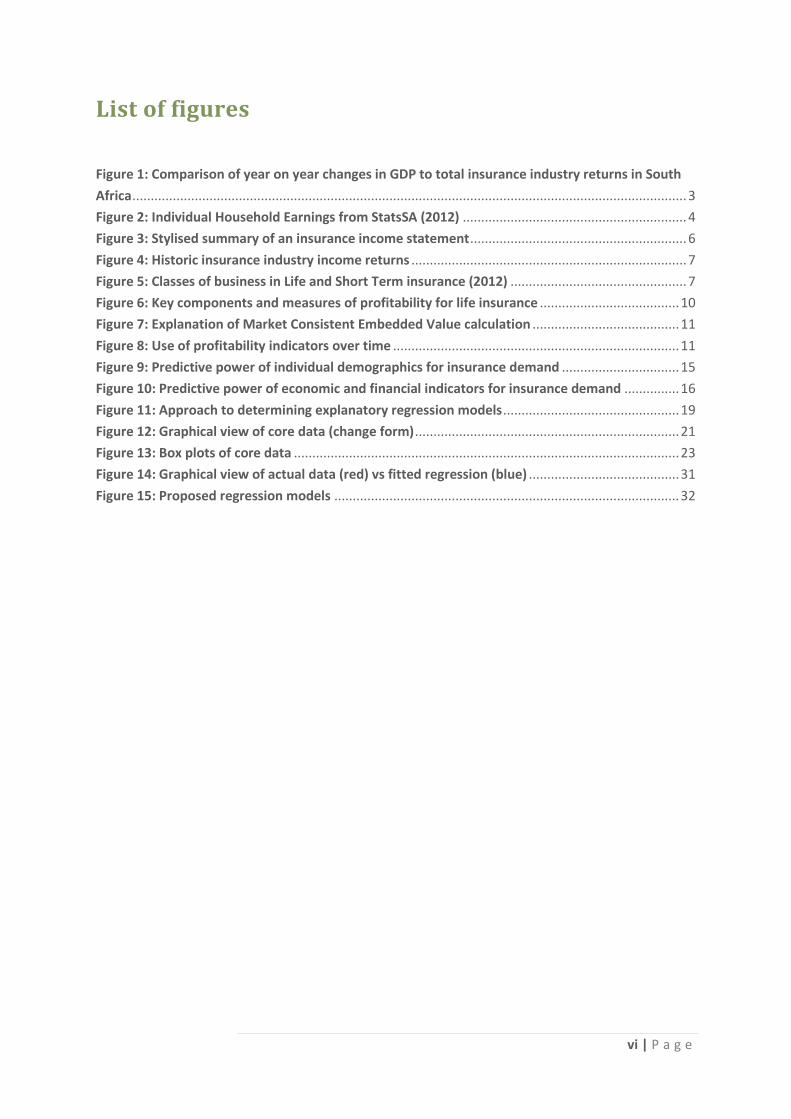
Figure 1 shows the annual change in underwriting performance of the South African Life
insurance industry relative to annual changes to GDP. GDP across all sectors as well as the finance,
real estate and business sector on its own were obtained from Statistics South Africa and annual
percentage changes calculated (StatsSA, 2014). Although the insurance returns show more volatility,
the movements between GDP and underwriting performance do seem to track together. This
suggests that insurance demand and performance (profitability), might be dependent on
macroeconomic factors and this hypothesis forms the basis for this study.
3 | P a g e
Source: FSB annual reports for Life and Short Term insurance, and Stats SA (FSB, 2014; StatsSA, 2014).
FIGURE 1: COMPARISON OF YEAR ON YEAR CHANGES IN GDP TO TOTAL INSURANCE INDUSTRY RETURNS
IN SOUTH AFRICA
1.2. Problem statement and research objectives
South African Life insurance markets include customers across a broad range of earnings. Figure
2 shows the monthly earnings of employed individuals across South Africa and highlights the range
of earnings, with the majority of individuals earning less than R 6 000 per month (Eighty20, 2014). It
is thus likely that insurance demand in this segment of the market is very sensitive to
macroeconomic factors, whereas demand from higher income individuals (> R 16 000 per month)
may follow macro-economic trends less closely. However, the actual empirical evidence for this is
unclear and this information seems vital, if not indispensable, for insurance companies to remain
profitable and sustainable. The earlier background context relating to determinants of demand for
insurance products makes this point strongly. These insights into demand would represent powerful
lead indicators for business planning and sales strategies.

4 | P a g e
Source: Eighty20 database (Eighty20, 2014)
FIGURE 2: INDIVIDUAL HOUSEHOLD EARNINGS FROM STATSSA (2012)
The aim of this research is thus to determine whether:
I. insurance demand and profitability in South Africa can be explained using a
macroeconomic model.
II. insurance demand in the low income market (individuals earning < R 6 000 per month)
can be explained differently from insurance demand in the higher income market
(individuals earning > R 16 000 per month) using macroeconomic factors.
1.3. Significance of study
By understanding the relationship between macroeconomic factors and insurance demand
(across income segments), insurance businesses are able to build forecasts accurately as well as gain
additional insights in terms of which business (products / customer segments) to promote or favour
based on the prevailing economic conditions. Understanding profiles of disparate income (economic)
groups and what differential products are most attractive to them would be a valuable knowledge.
1.4. Overview of methodology
1.4.1. Data
As discussed in the introduction, profitability is ultimately determined both by new business
growth as well as customer loyalty and longevity. In order to understand insurance demand and

5 | P a g e
profitability it thus makes sense to track three key metrics (policy sales, policy cancellations and
underwriting profit)
Sales data is an excellent proxy for insurance demand as it reflects buying behaviours of
consumers. Cancellations reflect policy off movements and relate to a consumer’s risk appetite,
brand loyalty and product features (e.g., affordability, perceived value). The underwriting margin
captures all of the above and is a good indicator of business sustainability.
Low income consumer data was collected from funeral policies, while the high net worth
consumer data was collected from underwritten Life products. Numerous macroeconomic indicators
are available to build the regression models (GDP, Repo Rate, CPI, Unemployment, Credit Standing
of consumers, Consumer enquiries for credit, Civil cases of debt, Financial Services confidence index,
Consumer Confidence). Their selection for this study is based on evidence within the literature that
they may influence insurance demand (Chui & Kwok, 2009; Doherty & Kang, 1988; Lee & Chiu, 2012;
Lee, Lee, & Chiu, 2013; Zietz, 2003).
1.4.2. Building the models
GRETL software was used to build all regressions and complete any relevant statistical analyses
(GRETL, 2014). In order to test whether macroeconomic factors influence insurance demand, six
different regression models have been determined. For each of the three insurance metrics (sales,
cancellations and underwriting profit) data was drawn from Life insurance sales for low income and
high net worth individuals. The best predictive model was then determined for each of these six
dependent variables using a bottom up approach as outlined in Chapter 3.
Although the insurance data is available on a monthly basis, the majority of macroeconomic
factors are published quarterly. Thus regression models using quarterly values of sales, cancellations
and underwriting profit were constructed, so as to compile a data set of uniform quarterly frequency
for the study.
1.5. Outline of research report
Following from this introduction is a detailed literature review, which provides an overview of
the insurance industry and explores in more detail which factors (demographic and economic)
influence insurance demand (Chapter 2). This leads to a description of the problem statement and
research objectives in Chapter 3, where the approach to collecting data and building regression
models to test the predictive power of macroeconomic factors on insurance demand is then
outlined. All of the descriptive statistics and model estimation data are then provided together with
an interpretation of the results in Chapter 4. Finally, the conclusions are presented and a list of
references provided in Chapters 5 and 6.
6 | P a g e
2. Literature Review
2.1. Insurance industry overview
The aim of this study is to better understand which key external drivers influence the insurance
industry and to then explore how they can be used in structuring and managing an insurance
company. This section summarises the key features (size, class of business, competitive landscape
and performance) of the insurance industry as a whole in South Africa and sets the context for a
more detailed description of what drives insurance demand at the end of this chapter.
The first documented evidence of Life insurance forms part of the Hammurabi Code, which
dates back to ancient Babylonian times (2500 BC). This code consists of 282 laws and includes
reference to basic insurance in that a debtor did not have to pay back his loans if some personal
catastrophe made it impossible to do so (Prince, 1904). Subsequently, stonemasons in Egypt are
believed to have formed funeral cooperatives to support each other in the event of death and
similar burial societies were common in India (1000 BC) and ancient Rome (Kirova & Steinmann,
2012).
Today the insurance industry is highly regulated and at the highest level distinction is made
between insurance policies which are short term in nature (renewable on an annual basis (Inseta,
2014)) versus those that have long term horizons (Life policies). Short Term insurance is divided into
seven classes of business (Property, Transportation, Motor, Accident & Health, Guarantee, Liability
and Engineering) (FSB, 2014). The Life industry includes four main classes of business (Investments,
Risk, Annuities and Universal Life).
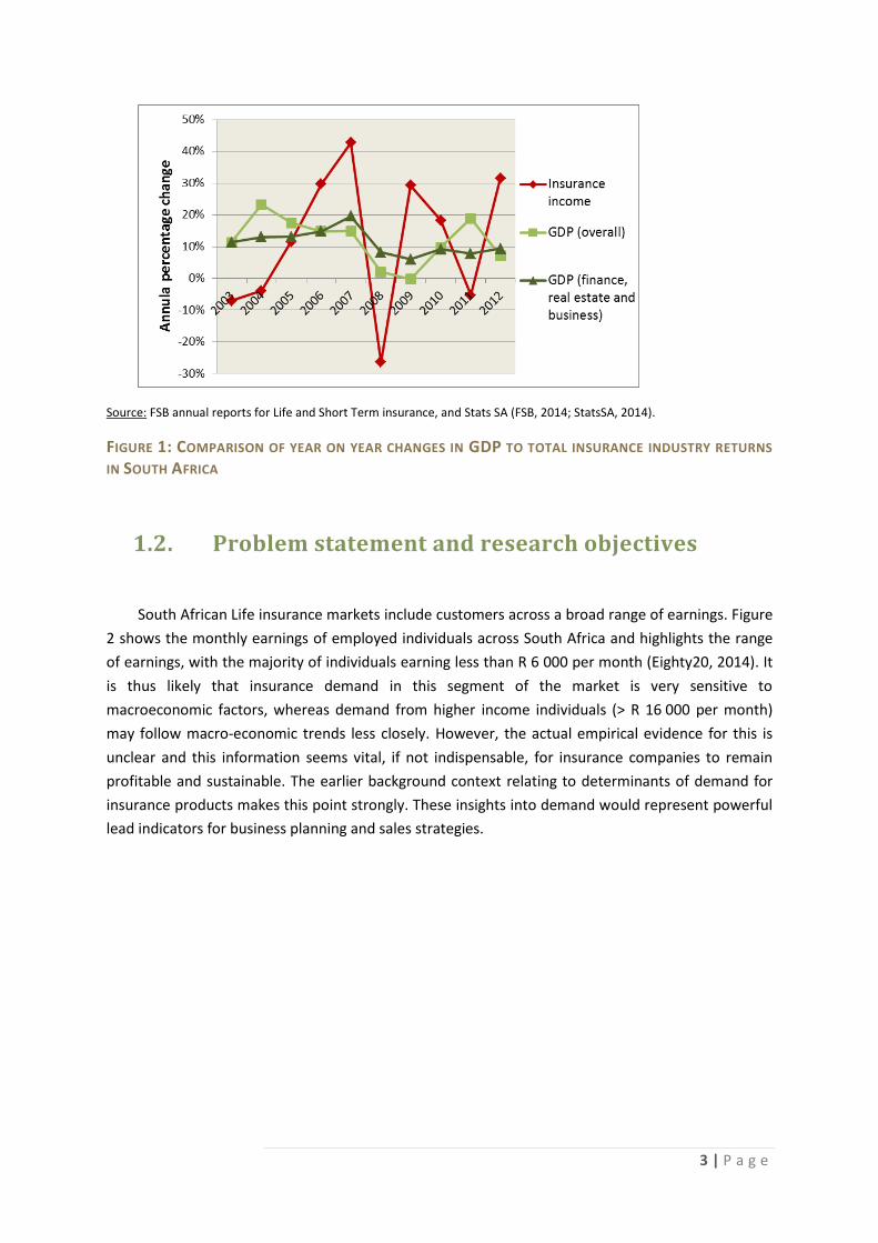
A high level summary of typical insurance revenues and costs is summarised in Figure 3.
Revenues are earned from the risk premium, asset fee income, inward reinsurance commissions and
investment income from holding the earned premium. Typical insurance costs include commissions
paid out to intermediaries such as brokers, policy administration costs, claims payments and other
expenses related to policy acquisition and marketing.
FIGURE 3: STYLISED SUMMARY OF AN INSURANCE INCOME STATEMENT
7 | P a g e
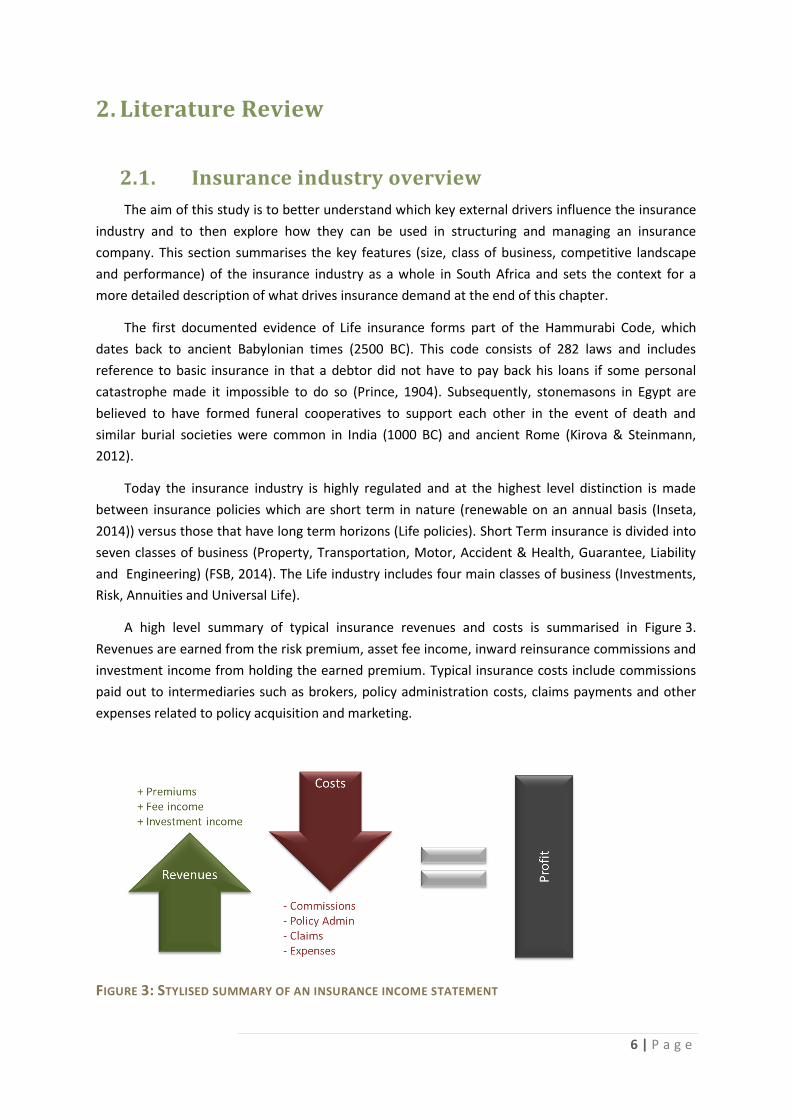
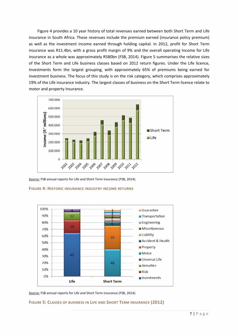
Figure 4 provides a 10 year history of total revenues earned between both Short Term and Life
insurance in South Africa. These revenues include the premium earned (insurance policy premium)
as well as the investment income earned through holding capital. In 2012, profit for Short Term
insurance was R11.4bn, with a gross profit margin of 9% and the overall operating Income for Life
insurance as a whole was approximately R580bn (FSB, 2014). Figure 5 summarises the relative sizes
of the Short Term and Life business classes based on 2012 return figures. Under the Life licence,
Investments form the largest grouping, with approximately 65% of premiums being earned for
investment business. The focus of this study is on the risk category, which comprises approximately
19% of the Life insurance industry. The largest classes of business on the Short Term licence relate to
motor and property insurance.
Source: FSB annual reports for Life and Short Term insurance (FSB, 2014).
FIGURE 4: HISTORIC INSURANCE INDUSTRY INCOME RETURNS
Source: FSB annual reports for Life and Short Term insurance (FSB, 2014).
FIGURE 5: CLASSES OF BUSINESS IN LIFE AND SHORT TERM INSURANCE (2012)
8 | P a g e
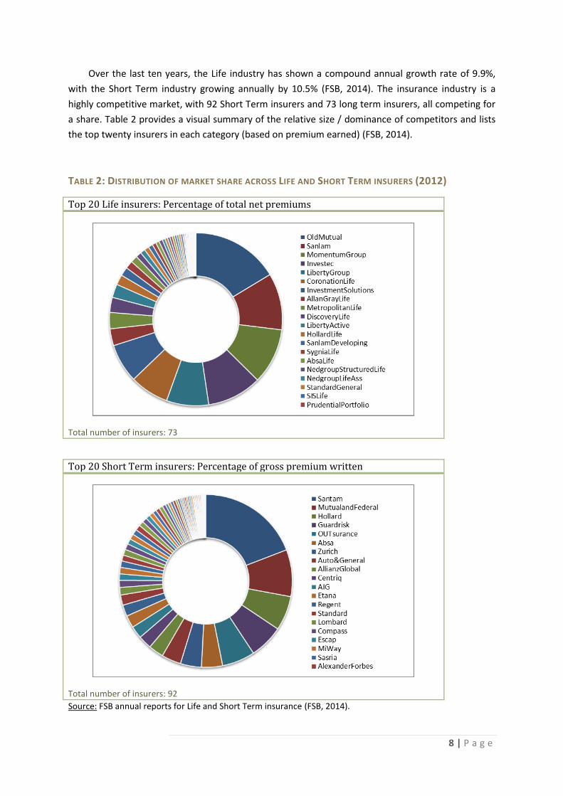
Over the last ten years, the Life industry has shown a compound annual growth rate of 9.9%,
with the Short Term industry growing annually by 10.5% (FSB, 2014). The insurance industry is a
highly competitive market, with 92 Short Term insurers and 73 long term insurers, all competing for
a share. Table 2 provides a visual summary of the relative size / dominance of competitors and lists
the top twenty insurers in each category (based on premium earned) (FSB, 2014).
TABLE 2: DISTRIBUTION OF MARKET SHARE ACROSS LIFE AND SHORT TERM INSURERS (2012)
Top 20 Life insurers: Percentage of total net premiums
Total number of insurers: 73
Top 20 Short Term insurers: Percentage of gross premium written
Total number of insurers: 92
Source: FSB annual reports for Life and Short Term insurance (FSB, 2014).

9 | P a g e
2.1.1. Insurance profitability drivers and measures
In general, companies aim to understand and track both internal and external business drivers
in order to maintain a competitive advantage in their respective markets. External business drivers
include overall economic performance and stability (public perceptions of the government,
institutional frameworks and governance) of the country in which you operate, labour resource
constraints such as skills, costs and availability as well as the overall market maturity and
competitive landscape (Barksdale & Lund, 2006). In emerging economies, such as South Africa, both
‘housekeeping’ (macro-policies, political environment, corporate governance and the maturity of
financial markets) and ‘plumbing’ factors (legal and regulatory frameworks and execution thereof)
are critical in establishing investor confidence (Ladekarl & Zervos, 2004). A strong understanding of
these factors and their impacts on business operations is essential for existing companies. In
addition to this, in emerging African economies capital structures often rely primarily on internal
finance and short term debt, which also impacts on business growth potential and profits (Gwatidzo
& Ojah, 2009).
External factors are often used as lead indicators to set or adjust business strategies and
operating models. Internal business drivers such as technology development / acquisition and
process design are often informed by external trends (Barksdale & Lund, 2006). Softer issues such a
shareholder management and leadership organisation (shaping the culture and managing change)
vary more across companies.
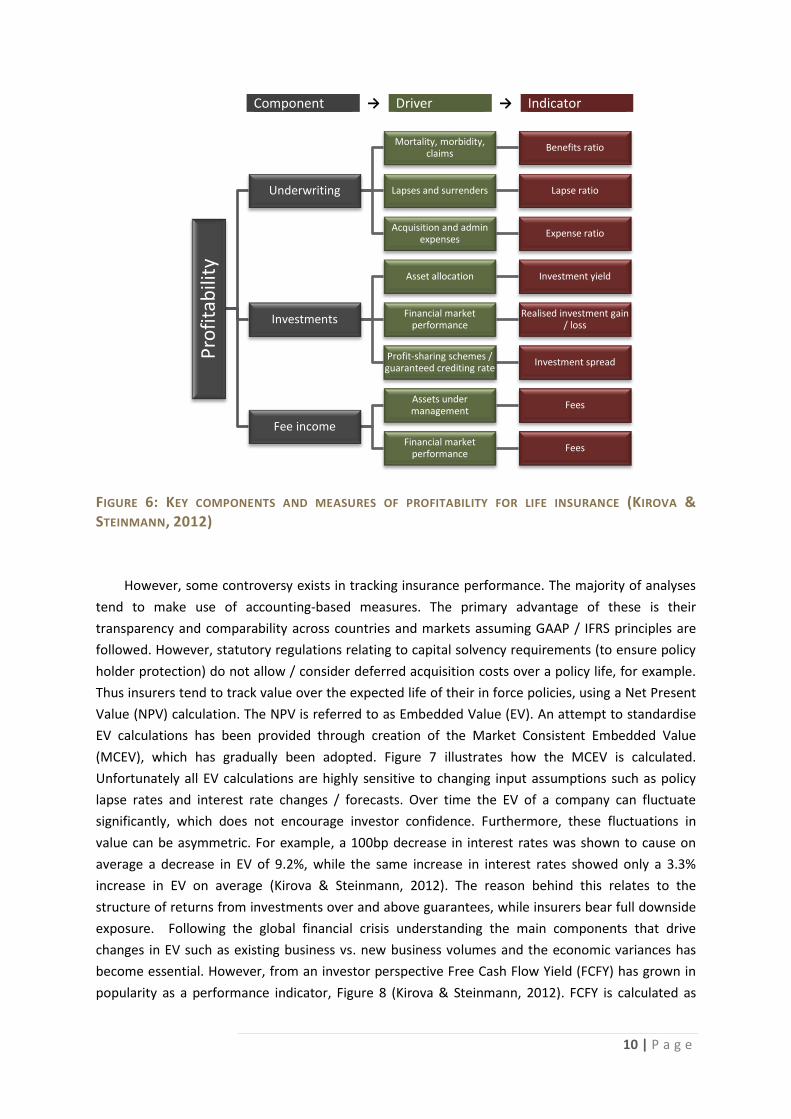
In the Life insurance industry there are three primary components to profit (underwriting
performance, investment returns and fee income). Figure 6 summarises these components and links
these to their respective key drivers and also provides economic indicators for each of these drivers.
Overall, business profitability has generally been tracked using accounting based ratios and analyses
such as total shareholder return, book value per share, price to book value, return on equity,
operating margin, return on assets and net investment results (Kirova & Steinmann, 2012). Historic
analyses have shown a close correlation between price to book ratios and earnings. This measure
effectively incorporates the exposure of overall profitability to stock market fluctuations. Return on
equity is more volatile than the price to book ratio, but is also a good proxy for performance and
there is a close correlation between these two benchmarks of performance (R2 = 0.727) (Kirova &
Steinmann, 2012).
10 | P a g e
Component → Driver → Indicator
FIGURE 6: KEY COMPONENTS AND MEASURES OF PROFITABILITY FOR LIFE INSURANCE (KIROVA &
STEINMANN, 2012)
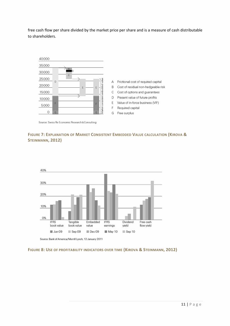
However, some controversy exists in tracking insurance performance. The majority of analyses
tend to make use of accounting-based measures. The primary advantage of these is their
transparency and comparability across countries and markets assuming GAAP / IFRS principles are
followed. However, statutory regulations relating to capital solvency requirements (to ensure policy
holder protection) do not allow / consider deferred acquisition costs over a policy life, for example.
Thus insurers tend to track value over the expected life of their in force policies, using a Net Present
Value (NPV) calculation. The NPV is referred to as Embedded Value (EV). An attempt to standardise
EV calculations has been provided through creation of the Market Consistent Embedded Value
(MCEV), which has gradually been adopted. Figure 7 illustrates how the MCEV is calculated.
Unfortunately all EV calculations are highly sensitive to changing input assumptions such as policy
lapse rates and interest rate changes / forecasts. Over time the EV of a company can fluctuate
significantly, which does not encourage investor confidence. Furthermore, these fluctuations in
value can be asymmetric. For example, a 100bp decrease in interest rates was shown to cause on
average a decrease in EV of 9.2%, while the same increase in interest rates showed only a 3.3%
increase in EV on average (Kirova & Steinmann, 2012). The reason behind this relates to the
structure of returns from investments over and above guarantees, while insurers bear full downside
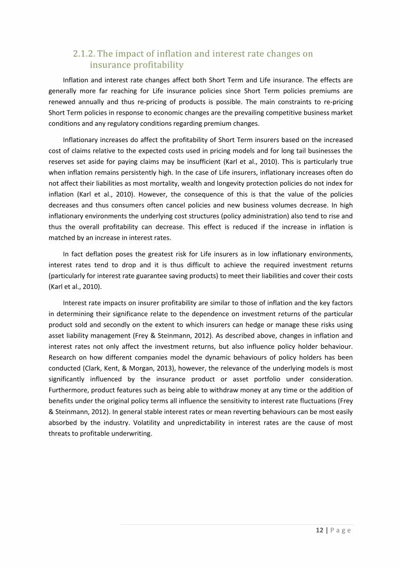
exposure. Following the global financial crisis understanding the main components that drive
changes in EV such as existing business vs. new business volumes and the economic variances has
become essential. However, from an investor perspective Free Cash Flow Yield (FCFY) has grown in
popularity as a performance indicator, Figure 8 (Kirova & Steinmann, 2012). FCFY is calculated as
Pro
fita
bili
ty
Underwriting
Mortality, morbidity, claims
Benefits ratio
Lapses and surrenders Lapse ratio
Acquisition and admin expenses
Expense ratio
Investments
Asset allocation Investment yield
Financial market performance
Realised investment gain / loss
Profit-sharing schemes / guaranteed crediting rate
Investment spread
Fee income
Assets under management
Fees
Financial market performance
Fees
11 | P a g e
free cash flow per share divided by the market price per share and is a measure of cash distributable
to shareholders.
FIGURE 7: EXPLANATION OF MARKET CONSISTENT EMBEDDED VALUE CALCULATION (KIROVA &
STEINMANN, 2012)
FIGURE 8: USE OF PROFITABILITY INDICATORS OVER TIME (KIROVA & STEINMANN, 2012)
12 | P a g e
2.1.2. The impact of inflation and interest rate changes on insurance profitability
Inflation and interest rate changes affect both Short Term and Life insurance. The effects are
generally more far reaching for Life insurance policies since Short Term policies premiums are
renewed annually and thus re-pricing of products is possible. The main constraints to re-pricing
Short Term policies in response to economic changes are the prevailing competitive business market
conditions and any regulatory conditions regarding premium changes.
Inflationary increases do affect the profitability of Short Term insurers based on the increased
cost of claims relative to the expected costs used in pricing models and for long tail businesses the
reserves set aside for paying claims may be insufficient (Karl et al., 2010). This is particularly true
when inflation remains persistently high. In the case of Life insurers, inflationary increases often do
not affect their liabilities as most mortality, wealth and longevity protection policies do not index for
inflation (Karl et al., 2010). However, the consequence of this is that the value of the policies
decreases and thus consumers often cancel policies and new business volumes decrease. In high
inflationary environments the underlying cost structures (policy administration) also tend to rise and
thus the overall profitability can decrease. This effect is reduced if the increase in inflation is
matched by an increase in interest rates.
In fact deflation poses the greatest risk for Life insurers as in low inflationary environments,
interest rates tend to drop and it is thus difficult to achieve the required investment returns
(particularly for interest rate guarantee saving products) to meet their liabilities and cover their costs
(Karl et al., 2010).
Interest rate impacts on insurer profitability are similar to those of inflation and the key factors
in determining their significance relate to the dependence on investment returns of the particular
product sold and secondly on the extent to which insurers can hedge or manage these risks using
asset liability management (Frey & Steinmann, 2012). As described above, changes in inflation and
interest rates not only affect the investment returns, but also influence policy holder behaviour.
Research on how different companies model the dynamic behaviours of policy holders has been
conducted (Clark, Kent, & Morgan, 2013), however, the relevance of the underlying models is most
significantly influenced by the insurance product or asset portfolio under consideration.
Furthermore, product features such as being able to withdraw money at any time or the addition of
benefits under the original policy terms all influence the sensitivity to interest rate fluctuations (Frey
& Steinmann, 2012). In general stable interest rates or mean reverting behaviours can be most easily
absorbed by the industry. Volatility and unpredictability in interest rates are the cause of most
threats to profitable underwriting.

13 | P a g e
2.2. State of the insurance industry in South Africa relative to Africa, emerging and developed economies
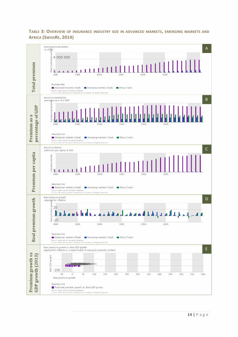
Table 3 provides a high level overview of the relative sizes of insurance in developed
economies, emerging markets as a whole and Africa (SwissRe, 2014). The relative dominance in size
of developed markets to both emerging economies and Africa is clear in panels A and C. Panel B
shows insurance premium expressed as a percentage of GDP and reveals a more promising view of
how the insurance industry has grown in the last 20 years in both emerging markets and Africa. This
growth (panel D), was most significant between 2000 and 2010, with emerging economies share of
the world’s GDP increasing from 21% to 34%, and in parallel total insurance premiums grew by 11%
annually in emerging economies, while insurance premiums only grew by 1.3% in industrialised
economies over this period (Kalra & Futterknecht, 2011).
Despite a global trend towards consolidation of markets and expansion of larger global insurers
into emerging economies, local insurers have outperformed their international counterparts in
emerging economies. This is largely due to richer consumer insights, the development of innovative,
tailored products (such as index-based weather insurance for agriculture) , control of distribution
channels (particularly leverage of bancassurance), and stable economic environments (low inflation)
(Kalra & Futterknecht, 2011).
Growth in insurance markets across Africa has been significant and is forecast to continue.
Table 4 provides a snapshot of a few African countries and their historic growth rates and market
composition. Although positive growth is forecast across most of these countries, the persistence of
low interest rates and new regulations (solvency regimes) is likely to dampen growth forecasts (Kalra
& Futterknecht, 2011).
TABLE 4: COMPARISON OF INSURANCE COMPETITIVE MARKET SIZE AND GROWTH IN AFRICA
Country Licence Number of insurers ⱡ Historic growth 2008-2012 (CAGR %)
South Africa Life 73 19.3 Short Term 92 6.1 Nigeria Life 16 10.1 Short Term 30 32.8 Kenya Life 11 17 Short Term 24 17.7 Ghana Life 18 19.1 Short Term 23 38.1 ⱡ Excludes composite insurance licences in Nigeria, Kenya and Ghana
14 | P a g e
TABLE 3: OVERVIEW OF INSURANCE INDUSTRY SIZE IN ADVANCED MARKETS, EMERGING MARKETS AND
AFRICA (SWISSRE, 2014) T
ota
l p
rem
ium
Pre
miu
m a
s a
p
erc
en
tag
e o
f G
DP
Pre
miu
m p
er
cap
ita
Re
al
pre
miu
m g
row
th
Pre
miu
m g
row
th v
s G
DP
gro
wth
(2
01
3)
A
B
C
D
E
15 | P a g e
2.3. Factors influencing insurance demand
As described in the introduction, a great deal of research has centred on developing models to
predict insurance demand relative to various risk aversion proxies. As with any model of human
behaviour it is not surprising that inconsistencies and deviations from expected or ‘rational’
behaviour are commonplace. Schwarcz (2010), describe four common categories of deviation from
theoretical risk aversion expectations: (i) bimodal demand for catastrophe (ignore high risk low
frequency events such as earthquakes), (ii) favour small financial risk, (iii) non-pecuniary benefit
preference, and (iv) low deductible preference.
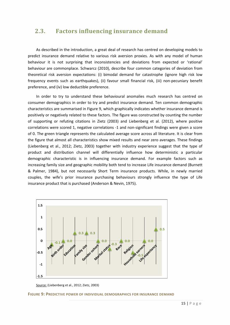
In order to try to understand these behavioural anomalies much research has centred on
consumer demographics in order to try and predict insurance demand. Ten common demographic
characteristics are summarised in Figure 9, which graphically indicates whether insurance demand is
positively or negatively related to these factors. The figure was constructed by counting the number
of supporting or refuting citations in Zietz (2003) and Liebenberg et al. (2012), where positive
correlations were scored 1, negative correlations -1 and non-significant findings were given a score
of 0. The green triangle represents the calculated average score across all literature. It is clear from
the figure that almost all characteristics show mixed results and near zero averages. These findings
(Liebenberg et al., 2012; Zietz, 2003) together with industry experience suggest that the type of
product and distribution channel will differentially influence how deterministic a particular
demographic characteristic is in influencing insurance demand. For example factors such as
increasing family size and geographic mobility both tend to increase Life insurance demand (Burnett
& Palmer, 1984), but not necessarily Short Term insurance products. While, in newly married
couples, the wife’s prior insurance purchasing behaviours strongly influence the type of Life
insurance product that is purchased (Anderson & Nevin, 1975).
Source: (Liebenberg et al., 2012; Zietz, 2003)
FIGURE 9: PREDICTIVE POWER OF INDIVIDUAL DEMOGRAPHICS FOR INSURANCE DEMAND

16 | P a g e
Over and above the individual’s risk aversion and demographic profiling, economic and financial
indicators have also been used to predict insurance demand (Zietz, 2003). These are less ambiguous
than demographic indicators as shown in Figure 10. The same analysis as for Figure 9 was followed
to construct Figure 10.
Source: (Zietz, 2003); ∆ Note: Stock market and credit card indices only include one reference each
FIGURE 10: PREDICTIVE POWER OF ECONOMIC AND FINANCIAL INDICATORS FOR INSURANCE DEMAND
The literature thus supports the contention that insurance demand is a function of individual
risk aversion, demographic characteristics which influence consumer attitudes and behaviours as
well as economic drivers. In running an insurance business, being able to plan and predict insurance
demand and ultimately to know which customers to target (acquisition and retention strategies) are
critical elements in structuring a profitable and sustainable business over time.
2.3.1. Key questions
It thus follows that it is of great interest and relevance to understand whether insurance
demand and profitability in South Africa can be explained using a macroeconomic model. A detailed
description and explanation of which factors are predictive of insurance demand (sales and
cancellations) and long term profitability, would allow proactive business strategies to be enacted. A
granular view of how individual consumer segments respond to macroeconomic changes would add
further insight and allow insurers to develop and structure their marketing and sales campaigns
based on both consumer needs and likely responsiveness.

17 | P a g e
3. Data and Methodology
3.1. Research objectives
The intention of this research study is to understand whether macroeconomic factors can
explain and ultimately act as lead indicators to predict insurance demand. Three factors are used as
proxies for insurance demand: i) new business sales, ii) policy cancellations and lapses and iii)
profitability. The latter refers more to business sustainability. The study also separated low income
consumers (individuals earning < R 6 000 per month) from the higher income market (individuals
earning > R 16 000 per month). The premise for this separation is to test whether lower income
consumers are more vulnerable / responsive to economic shifts.
3.2. Approach
3.2.1. Data
As discussed in the introduction, profitability is ultimately determined both by new business
growth as well as customer loyalty and longevity. In order to understand insurance demand and
profitability it thus makes sense to track three key metrics:
I. Policy sales
Sales are defined as those policies which are taken up by a customer and where a first
premium is collected
II. Policy cancellations
Cancellations for the purpose of this study are defined as when a customer actively
cancels a policy as well as when a policy lapses (and no premium is collected for three
successive months)
III. Underwriting profit
Underwriting profit refers to the insurance business profitability and represents income
earned after all insurance claims, actuarial reserving, operating expenses and direct
expenses are defrayed.
Sales data is an excellent proxy for insurance demand as it reflects buying behaviours of
consumers. Cancellations reflect policy off movements and relate to a consumer’s risk appetite,
brand loyalty and product features (e.g., affordability, perceived value). The underwriting margin
captures all of the above and is a good indicator of business sustainability.
All insurance data was collected from a single insurance company. Although the data was
available on a monthly basis, only quarterly data was collected to match the frequency of the

18 | P a g e
macroeconomic data set. Unfortunately, several changes to policy administrative systems across the
various books of business made collecting policy information earlier than January 2008 impossible.
Low income consumer data was collected from funeral policies sold through two direct to market
channels (non-advice), while the high net worth consumer data was collected from underwritten Life
products sold through brokers (advice). Although the distribution channels differ between the low
and high income consumers, the proposed study is only concerned with relative trends and not
absolute numbers of sales, cancellations and profitability, and so this is not deemed a material
difference.
Numerous macroeconomic indicators are available to build explanatory regression models.
Based on the literature review twelve indicators were identified and sourced for the purpose of this
study (Table 5) and their influence on insurance demand explored (Chui & Kwok, 2009; Doherty &
Kang, 1988; Lee & Chiu, 2012; Lee et al., 2013; Zietz, 2003).
TABLE 5: SUMMARY OF SOURCED ECONOMIC INDICATORS
Indicator Available data Frequency Source
GDP - Total at 2005 prices Jan 1993 – Jun 2014 Quarterly Stats SA
GDP-Finance, Real Estate, Bus Services at 2005 prices
Jan 1993 – Jun 2014 Quarterly Stats SA
Repo rate Jan 1982 – Jun 2014 Daily SARB
CPI00000 (Overall - 2012=100) Jan 2002 – Jun 2014 Monthly Stats SA
CPI12500 (Insurance - 2012=100) Jan 2002 – Jun 2014 Monthly Stats SA
Unemployment Jan 2008 – Jun 2014 Quarterly Stats SA
Civil cases recorded and summonses issued for debt (S1100000)
Jan 2000 – Jun 2014 Monthly Stats SA
Num Consumers with good credit standing Jun 2007 – Jun 2014 Quarterly NCR
Num Consumers with impaired records Jun 2007 – Jun 2014 Quarterly NCR
EY Financial Index (unweighted) Jan 2002 – Mar 2014 Quarterly Ernst & Young
EY Life Insurance index Jan 2002 – Mar 2014 Quarterly Ernst & Young
FNB-BER consumer confidence index Sep 1983 – Mar 2014 Quarterly BER / FNB
3.2.2. Building an explanatory model
Figure 11 provides a high level summary of the approach used to determine the most
descriptive regression model for each of the six dependent variables (Low and High income: sales,
cancellations and profits). Since the majority of macroeconomic variables are reported on a
quarterly basis, the models were built using quarterly data and in order to ensure that all variables
had similar units they were converted to quarterly change format [(Valuet - Valuet-1)/ Valuet-1].
Summary statistics were determined and the assumption that the data was normally distributed was
tested. Any independent variables showing high degrees of cross correlation were then rationalised
and only uncorrelated variables were used to build the subsequent regression models. Individual
regressions for each of these variables were calculated using the Ordinary Least Squares
methodology with GRETL software (GRETL, 2014). In each regression a constant plus one
independent variable was regressed against each of the six dependent variables. Since the intention

19 | P a g e
of the analysis was to build a predictive model, lags (zero to four) for each variable were also tested
individually and R2 values calculated.
Finally, a step wise approach was adopted to determine which combination of independent
variables best predicts each of the six dependent variables. The three variables with the highest R2
values were selected, combined sequentially and adjusted R2 values were calculated. The adjusted R2
is used as this approach ensures that only regressors which add to the explanatory power of the
model increase the R2 value (spurious regressors are excluded). The combination with the highest
adjusted R2 value was then noted as the optimal model.
Diagnostic tests, to ensure the underlying assumptions of the ordinary least squares approach
were not violated, were conducted. Initially all independent variables were tested for outliers and
whether they followed a normal distribution using the Grubbs and Doornik-Hansen tests,
respectively (Brooks, 2014; GraphPad Software, 2014). Once the proposed models were established
the residual error terms were tested for normality, heteroscedasticity (White’s test) and
autocorrelation (Bresch-Godfrey test). The overall robustness of each proposed model was also
tested by comparing the final outputs to an OLS regression, for each of the three dependent
variables (sales, cancellations and profits), which included all twelve original macroeconomic
variables.
FIGURE 11: APPROACH TO DETERMINING EXPLANATORY REGRESSION MODELS
Data
• Convert to change form: (Valuet - Valuet-1) / Valuet-1
Statistics
• Summary statistics
• Tests for normality and outliers
• Cross correlation of independent variables
Individual regressions
• Determine R2 values for each indpenedent variable with and without lags (L0, L1, L2, L3 and L4)
Descriptive model
•Combine variables and calculate optimal model (adjusted R2)
•Test statistics for normality, homoscedasticity and auctocorrelation

20 | P a g e
4. Results and Discussion
4.1. Descriptive statistics and diagnostic tests
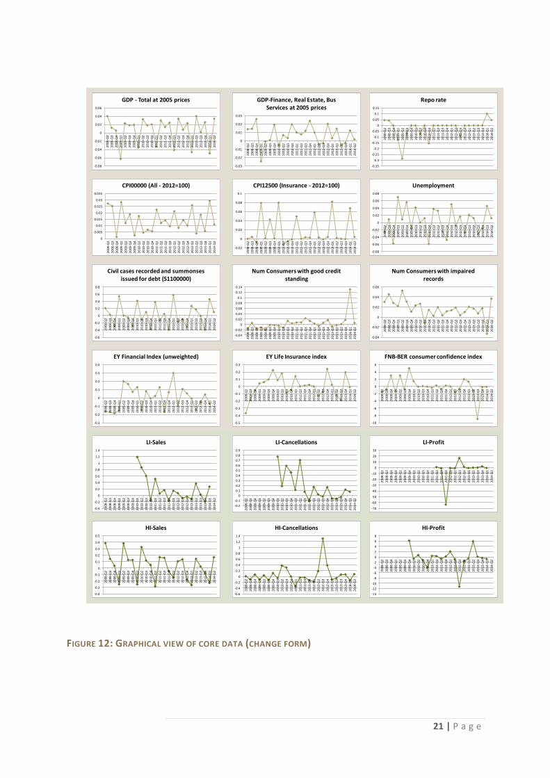
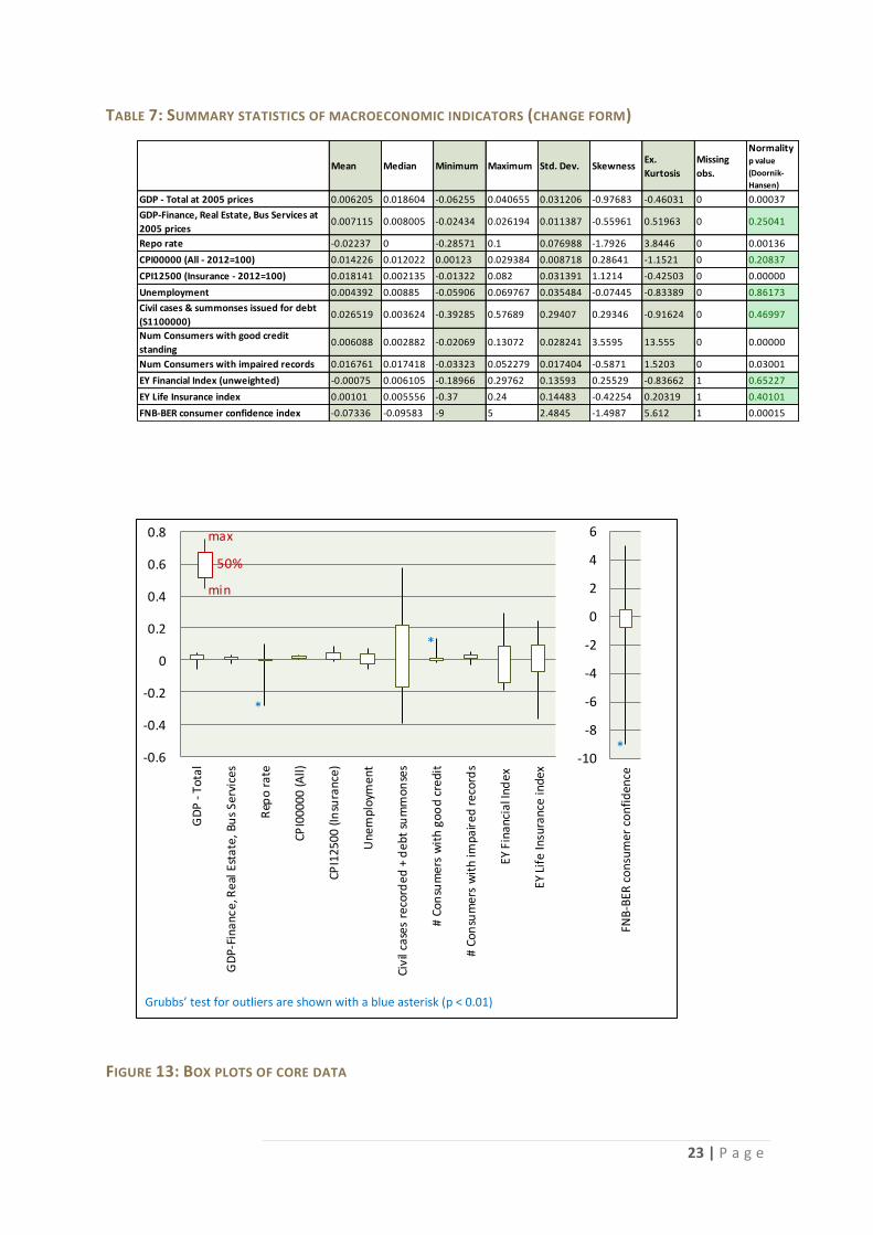
The core data used for this study is graphed in Figure 12 and summarised in Table 6. The
quarterly data was expressed in change format [(Valuet - Valuet-1)/ Valuet-1] to ensure that all
variables had similar units. Summary statistics for the test sample of regressors are provided in Table
7. All of the regressors have a mean close to zero and six are normally distributed based on the
Doornik-Hansen test (highlighted in green). The Grubbs’ test for sample outliers was also completed,
with three variables (repo rate, number of consumers with good credit standing and the FNB-BER
consumer confidence index) having statistically significant outliers, Figure 13 (GraphPad Software,
2014). Although outliers can skew OLS estimates, they do generally represent real events. For
example a spike in repo rate is not a spurious event and if it is in fact a valid predictor in a regression
model an outlier should not be excluded from an analysis. For this reason initial analyses included
all data from the independent variables even if an outlier was present.
In completing an ordinary least squares analysis five core assumptions of the underlying
regressors and residual error terms exist (Brooks, 2014):
1. Average value of error terms is zero
2. Variance of the error terms is constant (errors are homoscedastic)
3. Error terms are uncorrelated with each other (zero covariance)
4. Error terms are uncorrelated with the regressors
5. Error terms are normally distributed
In this study a constant term was included in all regressions, thus assumption 1 above was not
violated. In the final regression models several tests were used to test the other assumptions:
White’s test for heteroscedasticity, the Bresch-Godfrey test for autocorrelation of residuals (with up
to four lags) and the Doornik-Hansen test for normality.
21 | P a g e
FIGURE 12: GRAPHICAL VIEW OF CORE DATA (CHANGE FORM)
-0.08
-0.06
-0.04
-0.02
0
0.02
0.04
0.062
008
-Q2
20
08-Q
3
20
08-Q
4
20
09-Q
1
20
09-Q
2
20
09-Q
3
20
09-Q
4
20
10-Q
1
20
10-Q
2
20
10-Q
3
20
10-Q
4
20
11-Q
1
20
11-Q
2
20
11-Q
3
20
11-Q
4
20
12-Q
1
20
12-Q
2
20
12-Q
3
20
12-Q
4
20
13-Q
1
20
13-Q
2
20
13-Q
3
20
13-Q
4
20
14-Q
1
20
14-Q
2
GDP - Total at 2005 prices
-0.03
-0.02
-0.01
0
0.01
0.02
0.03
20
08-Q
2
20
08-Q
3
20
08-Q
4
20
09-Q
1
20
09-Q
2
20
09-Q
3
20
09-Q
4
20
10-Q
1
20
10-Q
2
20
10-Q
3
20
10-Q
4
20
11-Q
1
20
11-Q
2
20
11-Q
3
20
11-Q
4
20
12-Q
1
20
12-Q
2
20
12-Q
3
20
12-Q
4
20
13-Q
1
20
13-Q
2
20
13-Q
3
20
13-Q
4
20
14-Q
1
20
14-Q
2
GDP-Finance, Real Estate, Bus Services at 2005 prices
0
0.005
0.01
0.015
0.02
0.025
0.03
0.035
20
08-Q
2
20
08-Q
3
20
08-Q
4
20
09-Q
1
20
09-Q
2
20
09-Q
3
20
09-Q
4
20
10-Q
1
20
10-Q
2
20
10-Q
3
20
10-Q
4
20
11-Q
1
20
11-Q
2
20
11-Q
3
20
11-Q
4
20
12-Q
1
20
12-Q
2
20
12-Q
3
20
12-Q
4
20
13-Q
1
20
13-Q
2
20
13-Q
3
20
13-Q
4
20
14-Q
1
20
14-Q
2
CPI00000 (All - 2012=100)
-0.02
0
0.02
0.04
0.06
0.08
0.1
20
08-Q
2
20
08-Q
3
20
08-Q
4
20
09-Q
1
20
09-Q
2
20
09-Q
3
20
09-Q
4
20
10-Q
1
20
10-Q
2
20
10-Q
3
20
10-Q
4
20
11-Q
1
20
11-Q
2
20
11-Q
3
20
11-Q
4
20
12-Q
1
20
12-Q
2
20
12-Q
3
20
12-Q
4
20
13-Q
1
20
13-Q
2
20
13-Q
3
20
13-Q
4
20
14-Q
1
20
14-Q
2
CPI12500 (Insurance - 2012=100)
-0.6
-0.4
-0.2
0
0.2
0.4
0.6
0.8
20
08-Q
2
20
08-Q
3
20
08-Q
4
20
09-Q
1
20
09-Q
2
20
09-Q
3
20
09-Q
4
20
10-Q
1
20
10-Q
2
20
10-Q
3
20
10-Q
4
20
11-Q
1
20
11-Q
2
20
11-Q
3
20
11-Q
4
20
12-Q
1
20
12-Q
2
20
12-Q
3
20
12-Q
4
20
13-Q
1
20
13-Q
2
20
13-Q
3
20
13-Q
4
20
14-Q
1
20
14-Q
2
Civil cases recorded and summonses issued for debt (S1100000)
-0.04
-0.02
0
0.02
0.04
0.06
0.08
0.1
0.12
0.14
20
08-Q
2
20
08-Q
3
20
08-Q
4
20
09-Q
1
20
09-Q
2
20
09-Q
3
20
09-Q
4
20
10-Q
1
20
10-Q
2
20
10-Q
3
20
10-Q
4
20
11-Q
1
20
11-Q
2
20
11-Q
3
20
11-Q
4
20
12-Q
1
20
12-Q
2
20
12-Q
3
20
12-Q
4
20
13-Q
1
20
13-Q
2
20
13-Q
3
20
13-Q
4
20
14-Q
1
20
14-Q
2
Num Consumers with good credit standing
-0.35
-0.3
-0.25
-0.2
-0.15
-0.1
-0.05
0
0.05
0.1
0.15
20
08-Q
2
20
08-Q
3
20
08-Q
4
20
09-Q
1
20
09-Q
2
20
09-Q
3
20
09-Q
4
20
10-Q
1
20
10-Q
2
20
10-Q
3
20
10-Q
4
20
11-Q
1
20
11-Q
2
20
11-Q
3
20
11-Q
4
20
12-Q
1
20
12-Q
2
20
12-Q
3
20
12-Q
4
20
13-Q
1
20
13-Q
2
20
13-Q
3
20
13-Q
4
20
14-Q
1
20
14-Q
2
Repo rate
-0.08
-0.06
-0.04
-0.02
0
0.02
0.04
0.06
0.08
20
08-Q
2
20
08-Q
3
20
08-Q
4
20
09-Q
1
20
09-Q
2
20
09-Q
3
20
09-Q
4
20
10-Q
1
20
10-Q
2
20
10-Q
3
20
10-Q
4
20
11-Q
1
20
11-Q
2
20
11-Q
3
20
11-Q
4
20
12-Q
1
20
12-Q
2
20
12-Q
3
20
12-Q
4
20
13-Q
1
20
13-Q
2
20
13-Q
3
20
13-Q
4
20
14-Q
1
20
14-Q
2
Unemployment
-0.04
-0.02
0
0.02
0.04
0.06
20
08-Q
2
20
08-Q
3
20
08-Q
4
20
09-Q
1
20
09-Q
2
20
09-Q
3
20
09-Q
4
20
10-Q
1
20
10-Q
2
20
10-Q
3
20
10-Q
4
20
11-Q
1
20
11-Q
2
20
11-Q
3
20
11-Q
4
20
12-Q
1
20
12-Q
2
20
12-Q
3
20
12-Q
4
20
13-Q
1
20
13-Q
2
20
13-Q
3
20
13-Q
4
20
14-Q
1
20
14-Q
2
Num Consumers with impaired records
-0.3
-0.2
-0.1
0
0.1
0.2
0.3
0.4
20
08-Q
2
20
08-Q
3
20
08-Q
4
20
09-Q
1
20
09-Q
2
20
09-Q
3
20
09-Q
4
20
10-Q
1
20
10-Q
2
20
10-Q
3
20
10-Q
4
20
11-Q
1
20
11-Q
2
20
11-Q
3
20
11-Q
4
20
12-Q
1
20
12-Q
2
20
12-Q
3
20
12-Q
4
20
13-Q
1
20
13-Q
2
20
13-Q
3
20
13-Q
4
20
14-Q
1
20
14-Q
2
EY Financial Index (unweighted)
-0.5
-0.4
-0.3
-0.2
-0.1
0
0.1
0.2
0.3
20
08-Q
2
20
08-Q
3
20
08-Q
4
20
09-Q
1
20
09-Q
2
20
09-Q
3
20
09-Q
4
20
10-Q
1
20
10-Q
2
20
10-Q
3
20
10-Q
4
20
11-Q
1
20
11-Q
2
20
11-Q
3
20
11-Q
4
20
12-Q
1
20
12-Q
2
20
12-Q
3
20
12-Q
4
20
13-Q
1
20
13-Q
2
20
13-Q
3
20
13-Q
4
20
14-Q
1
20
14-Q
2EY Life Insurance index
-10
-8
-6
-4
-2
0
2
4
6
20
08-Q
2
20
08-Q
3
20
08-Q
4
20
09-Q
1
20
09-Q
2
20
09-Q
3
20
09-Q
4
20
10-Q
1
20
10-Q
2
20
10-Q
3
20
10-Q
4
20
11-Q
1
20
11-Q
2
20
11-Q
3
20
11-Q
4
20
12-Q
1
20
12-Q
2
20
12-Q
3
20
12-Q
4
20
13-Q
1
20
13-Q
2
20
13-Q
3
20
13-Q
4
20
14-Q
1
20
14-Q
2
FNB-BER consumer confidence index
-0.4
-0.2
0
0.2
0.4
0.6
0.8
1
1.2
1.4
20
08-Q
2
20
08-Q
3
20
08-Q
4
20
09-Q
1
20
09-Q
2
20
09-Q
3
20
09-Q
4
20
10-Q
1
20
10-Q
2
20
10-Q
3
20
10-Q
4
20
11-Q
1
20
11-Q
2
20
11-Q
3
20
11-Q
4
20
12-Q
1
20
12-Q
2
20
12-Q
3
20
12-Q
4
20
13-Q
1
20
13-Q
2
20
13-Q
3
20
13-Q
4
20
14-Q
1
20
14-Q
2
LI-Sales
-0.2
-0.1
0
0.1
0.2
0.3
0.4
0.5
0.6
0.7
0.8
0.9
20
08-Q
2
20
08-Q
3
20
08-Q
4
20
09-Q
1
20
09-Q
2
20
09-Q
3
20
09-Q
4
20
10-Q
1
20
10-Q
2
20
10-Q
3
20
10-Q
4
20
11-Q
1
20
11-Q
2
20
11-Q
3
20
11-Q
4
20
12-Q
1
20
12-Q
2
20
12-Q
3
20
12-Q
4
20
13-Q
1
20
13-Q
2
20
13-Q
3
20
13-Q
4
20
14-Q
1
20
14-Q
2
LI-Cancellations
-70
-60
-50
-40
-30
-20
-10
0
10
20
30
20
08-Q
2
20
08-Q
3
20
08-Q
4
20
09-Q
1
20
09-Q
2
20
09-Q
3
20
09-Q
4
20
10-Q
1
20
10-Q
2
20
10-Q
3
20
10-Q
4
20
11-Q
1
20
11-Q
2
20
11-Q
3
20
11-Q
4
20
12-Q
1
20
12-Q
2
20
12-Q
3
20
12-Q
4
20
13-Q
1
20
13-Q
2
20
13-Q
3
20
13-Q
4
20
14-Q
1
20
14-Q
2
LI-Profit
-0.4
-0.3
-0.2
-0.1
0
0.1
0.2
0.3
0.4
0.5
20
08-Q
2
20
08-Q
3
20
08-Q
4
20
09-Q
1
20
09-Q
2
20
09-Q
3
20
09-Q
4
20
10-Q
1
20
10-Q
2
20
10-Q
3
20
10-Q
4
20
11-Q
1
20
11-Q
2
20
11-Q
3
20
11-Q
4
20
12-Q
1
20
12-Q
2
20
12-Q
3
20
12-Q
4
20
13-Q
1
20
13-Q
2
20
13-Q
3
20
13-Q
4
20
14-Q
1
20
14-Q
2
HI-Sales
-0.6
-0.4
-0.2
0
0.2
0.4
0.6
0.8
1
1.2
1.4
20
08-Q
2
20
08-Q
3
20
08-Q
4
20
09-Q
1
20
09-Q
2
20
09-Q
3
20
09-Q
4
20
10-Q
1
20
10-Q
2
20
10-Q
3
20
10-Q
4
20
11-Q
1
20
11-Q
2
20
11-Q
3
20
11-Q
4
20
12-Q
1
20
12-Q
2
20
12-Q
3
20
12-Q
4
20
13-Q
1
20
13-Q
2
20
13-Q
3
20
13-Q
4
20
14-Q
1
20
14-Q
2
HI-Cancellations
-14
-12
-10
-8
-6
-4
-2
0
2
4
6
8
20
08-Q
2
20
08-Q
3
20
08-Q
4
20
09-Q
1
20
09-Q
2
20
09-Q
3
20
09-Q
4
20
10-Q
1
20
10-Q
2
20
10-Q
3
20
10-Q
4
20
11-Q
1
20
11-Q
2
20
11-Q
3
20
11-Q
4
20
12-Q
1
20
12-Q
2
20
12-Q
3
20
12-Q
4
20
13-Q
1
20
13-Q
2
20
13-Q
3
20
13-Q
4
20
14-Q
1
20
14-Q
2
HI-Profit

22 | P a g e
TABLE 6: CORE DATA USED FOR ANALYSIS (CHANGE FORM)
GDP - Total at
2005 prices
GDP-
Finance,
Real Estate,
Bus Services
at 2005
prices
Repo rate
CPI00000
(All -
2012=100)
CPI12500
(Insurance -
2012=100)
Unemploym
ent
Civil cases
recorded
and
summonses
issued for
debt
(S1100000)
Num
Consumers
with good
credit
standing
Num
Consumers
with
impaired
records
EY Financial
Index
(unweighted
)
EY Life
Insurance
index
FNB-BER
consumer
confidence
index
SalesCancellation
sProfit Sales
Cancellation
sProfit
2008-Q2 0.04062776 0.013958 0.045455 0.027202 0 -0.02586 0.212763 -0.01611 0.030349 -0.16667 -0.37 -1.5 0.386836 0.009399
2008-Q3 0.01183882 0.014499 0.043478 0.025221 0.004005 0.00885 0.021247 0.004817 0.045655 -0.17143 -0.19048 -0.83333 0.140139 -0.09622
2008-Q4 0.00552237 0.026194 0 0.00123 -0.00798 -0.05702 -0.2863 -0.0163 0.028169 -0.18966 -0.05882 3 0.03279 0.060103
2009-Q1 -0.0625488 -0.02434 -0.125 0.028256 0.079088 0.069767 0.537568 -0.01072 0.021918 -0.14894 0.041667 -1.25 -0.2538 -0.10799
2009-Q2 0.02324473 -0.00084 -0.28571 0.011947 0.001242 0.008696 0.003624 -0.02069 0.052279 0.2 0.06 3 0.383185 0.030872
2009-Q3 0.0186036 0.00103 -0.06667 0.01889 0.042184 0.056034 -0.04834 -0.00201 0.030573 0.166667 0.09434 -0.75 0.125806 -0.12331
2009-Q4 0.01879962 0.01936 0 0.002317 0.00119 -0.01633 -0.28176 -0.00302 0.011125 0.071429 0.224138 5 0.125327 0.119223 6.128262
2010-Q1 -0.0359708 -0.00506 0 0.017341 0.079667 0.041494 0.412906 -0.00506 0.023227 0 0.084507 1.5 1.187874 0.769437 -0.25167 -0.05566 -0.66321
2010-Q2 0.03239847 0.006925 -0.07143 0.004545 -0.01322 0 -0.11343 -0.01118 0.026284 0 0.181818 -0.06667 0.863456 0.183712 0.323295 0.370089 0.682204
2010-Q3 0.01817457 0.003425 0 0.006787 -0.00558 0.011952 0.098607 0.013361 -0.01164 0 -0.08791 0.071429 0.600834 0.59008 0.117898 0.309898 -1.15138
2010-Q4 0.02033851 0.019731 -0.15385 0.005618 -0.00112 -0.05906 -0.37594 0.004057 0.014134 0 -0.04819 -0.06667 -0.15237 0.457637 0.044917 -0.00812 -4.0668
2011-Q1 -0.0330084 0.010157 0 0.022346 0.049438 0.037657 0.37661 0.007071 0.002323 0.020243 0.139241 -0.35714 0.512198 0.109347 -0.28544 -0.34781 0.354156
2011-Q2 0.03019316 0.008005 0 0.012022 0 0.032258 -0.13249 0.007021 0.019699 0 0 0.222222 0.052219 0.700933 0.620929 0.168162 -0.04258 0.294041
2011-Q3 0.01412334 0.012046 0 0.014039 0.003212 -0.02344 0.042725 0.022908 0.003409 0 0.011111 -0.63636 0.159654 0.075108 -1.022 0.159012 -0.0382 -0.61874
2011-Q4 0.02403349 0.023965 0 0.009585 0.002134 -0.048 -0.39285 0.013632 0.011325 0.067797 0.021978 0.25 -0.16526 -0.10767 -63.5393 -0.043 -0.14464 0.117737
2012-Q1 -0.0417441 0.010213 0 0.021097 0.058573 0.05042 0.576891 0.002882 0.013438 0 0 0 0.148167 0.170842 -0.52555 -0.14933 -0.18503 2.062553
2012-Q2 0.03385722 -0.00425 0 0.008264 0.003018 -0.008 -0.16838 -0.00575 0.018785 0 0 -1.6 0.069489 0.022864 -0.89386 0.103415 0.180272 -0.87424
2012-Q3 0.00775881 -0.0027 -0.09091 0.014344 -0.001 0.016129 -0.10365 0.006744 0.003254 0 0 -0.66667 -0.08028 -0.02223 16.26215 0.133208 1.303314 -11.2967
2012-Q4 0.02295978 0.020425 0 0.010101 0.004016 -0.02778 -0.31392 0.016268 0.00973 0 0.24 2 -0.0352 0.163709 1.473498 -0.1783 0.38411 -1.61844
2013-Q1 -0.0464836 0.003146 0 0.026 0.082 0.020408 0.272406 -0.00659 0.020343 0 0.021505 1.333333 -0.10877 -0.0591 -0.66731 -0.26437 -0.10938 -0.596
2013-Q2 0.04065541 0.014663 0 0.003899 0.001848 0.012 0.169651 -0.00284 0.016789 -0.1437 -0.12632 -1.14286 0.366188 -0.06308 -0.30788 0.14147 -0.05658 5.92819
2013-Q3 0.00145442 -0.00503 0 0.018447 0 -0.03162 -0.00889 0.000951 0.007224 0 0 -9 0.020603 -0.03095 -0.13284 0.021643 0.058634 0.077053
2013-Q4 0.02534008 -0.00192 0 0.00572 -0.00092 -0.01633 -0.39258 0.017094 0.017418 0.039711 0.19403 -0.125 -0.19841 0.118325 1.993128 -0.07804 0.066311 -0.43659
2014-Q1 -0.049038 0.012331 0.1 0.029384 0.067405 0.045643 0.454516 0.130719 -0.03323 0 -0.0125 -0.14286 0.265342 0.071943 -0.51513 -0.22958 -0.14201 -0.70681
2014-Q2 0.03399878 0.001928 0.045455 0.01105 0.004325 0.011905 0.101976 0.004955 0.036458 0.166709 0.082199
Dependent variables
Low income High IncomeIndependent variables
23 | P a g e
TABLE 7: SUMMARY STATISTICS OF MACROECONOMIC INDICATORS (CHANGE FORM)
Grubbs’ test for outliers are shown with a blue asterisk (p < 0.01)
FIGURE 13: BOX PLOTS OF CORE DATA
Mean Median Minimum Maximum Std. Dev. SkewnessEx.
Kurtosis
Missing
obs.
Normality p value
(Doornik-
Hansen)
GDP - Total at 2005 prices 0.006205 0.018604 -0.06255 0.040655 0.031206 -0.97683 -0.46031 0 0.00037
GDP-Finance, Real Estate, Bus Services at
2005 prices0.007115 0.008005 -0.02434 0.026194 0.011387 -0.55961 0.51963 0 0.25041
Repo rate -0.02237 0 -0.28571 0.1 0.076988 -1.7926 3.8446 0 0.00136
CPI00000 (All - 2012=100) 0.014226 0.012022 0.00123 0.029384 0.008718 0.28641 -1.1521 0 0.20837
CPI12500 (Insurance - 2012=100) 0.018141 0.002135 -0.01322 0.082 0.031391 1.1214 -0.42503 0 0.00000
Unemployment 0.004392 0.00885 -0.05906 0.069767 0.035484 -0.07445 -0.83389 0 0.86173
Civil cases & summonses issued for debt
(S1100000)0.026519 0.003624 -0.39285 0.57689 0.29407 0.29346 -0.91624 0 0.46997
Num Consumers with good credit
standing0.006088 0.002882 -0.02069 0.13072 0.028241 3.5595 13.555 0 0.00000
Num Consumers with impaired records 0.016761 0.017418 -0.03323 0.052279 0.017404 -0.5871 1.5203 0 0.03001
EY Financial Index (unweighted) -0.00075 0.006105 -0.18966 0.29762 0.13593 0.25529 -0.83662 1 0.65227
EY Life Insurance index 0.00101 0.005556 -0.37 0.24 0.14483 -0.42254 0.20319 1 0.40101
FNB-BER consumer confidence index -0.07336 -0.09583 -9 5 2.4845 -1.4987 5.612 1 0.00015
-0.6
-0.4
-0.2
0
0.2
0.4
0.6
0.8
GD
P -
To
tal
GD
P-F
inan
ce, R
eal E
stat
e, B
us
Serv
ices
Rep
o r
ate
CP
I00
00
0 (
All
)
CP
I12
50
0 (I
nsu
ran
ce)
Une
mpl
oym
ent
Civ
il ca
ses
reco
rded
+ d
ebt
sum
mo
nse
s
# C
on
sum
ers
wit
h g
oo
d c
red
it
# C
on
sum
ers
wit
h im
pai
red
rec
ord
s
EY F
inan
cial
Ind
ex
EY L
ife
Insu
ranc
e in
dex
50%
max
min
-10
-8
-6
-4
-2
0
2
4
6
FNB
-BER
co
nsu
mer
co
nfi
den
ce
*
*
*

24 | P a g e
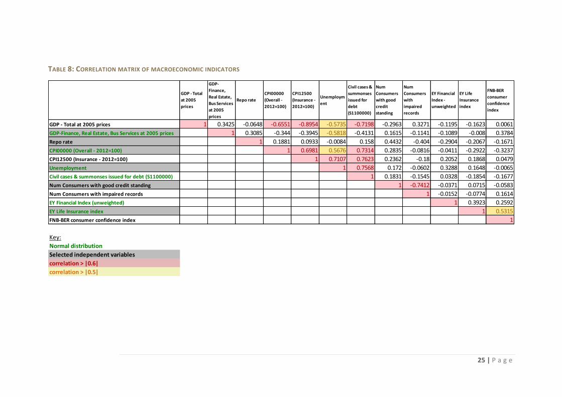
Table 8 represents a correlation matrix for the independent variables used in this study. All
correlations greater than |0.5| were noted. Based on the findings the overall number of
independent variables used in the study was reduced from twelve to six. Where possible, normally
distributed variables were selected. For example total CPI and CPI for insurance are correlated (0.7),
but only total CPI is normally distributed and thus this variable selected for the study. In summary
the following independent variables were selected and used for all subsequent regression analyses:
CPI00000 (Overall - 2012=100)
EY Life Insurance index
GDP-Finance, Real Estate, Bus Services (2005)
Number of consumers with good credit standing
Repo rate
Unemployment
Only the repo rate and number of consumers with good credit standing were not normally
distributed.
Based on this revised universe of independent variables, the next step in building a predictive
regression model was to determine which of the independent variables had the most explanatory
power for each of the six dependent variables. For each of the six dependent variables a regression
(ordinary least squares) with each independent variable was conducted and the R2 value captured.
All regressions included a constant term as well as separate lags from zero to four. Thus a total of
180 individual regressions were performed and are summarised in Table 9. Significant R2 values are
highlighted in the table and the highest R2 value per variable is highlighted with a red box.
25 | P a g e
TABLE 8: CORRELATION MATRIX OF MACROECONOMIC INDICATORS
GDP - Total
at 2005
prices
GDP-
Finance,
Real Estate,
Bus Services
at 2005
prices
Repo rate
CPI00000
(Overall -
2012=100)
CPI12500
(Insurance -
2012=100)
Unemploym
ent
Civil cases &
summonses
issued for
debt
(S1100000)
Num
Consumers
with good
credit
standing
Num
Consumers
with
impaired
records
EY Financial
Index -
unweighted
EY Life
Insurance
index
FNB-BER
consumer
confidence
index
GDP - Total at 2005 prices 1 0.3425 -0.0648 -0.6551 -0.8954 -0.5735 -0.7198 -0.2963 0.3271 -0.1195 -0.1623 0.0061
GDP-Finance, Real Estate, Bus Services at 2005 prices 1 0.3085 -0.344 -0.3945 -0.5818 -0.4131 0.1615 -0.1141 -0.1089 -0.008 0.3784
Repo rate 1 0.1881 0.0933 -0.0084 0.158 0.4432 -0.404 -0.2904 -0.2067 -0.1671
CPI00000 (Overall - 2012=100) 1 0.6981 0.5676 0.7314 0.2835 -0.0816 -0.0411 -0.2922 -0.3237
CPI12500 (Insurance - 2012=100) 1 0.7107 0.7623 0.2362 -0.18 0.2052 0.1868 0.0479
Unemployment 1 0.7568 0.172 -0.0602 0.3288 0.1648 -0.0065
Civil cases & summonses issued for debt (S1100000) 1 0.1831 -0.1545 0.0328 -0.1854 -0.1677
Num Consumers with good credit standing 1 -0.7412 -0.0371 0.0715 -0.0583
Num Consumers with impaired records 1 -0.0152 -0.0774 0.1614
EY Financial Index (unweighted) 1 0.3923 0.2592
EY Life Insurance index 1 0.5315
FNB-BER consumer confidence index 1
Key:
Normal distribution
Selected independent variables
correlation > |0.6|
correlation > |0.5|
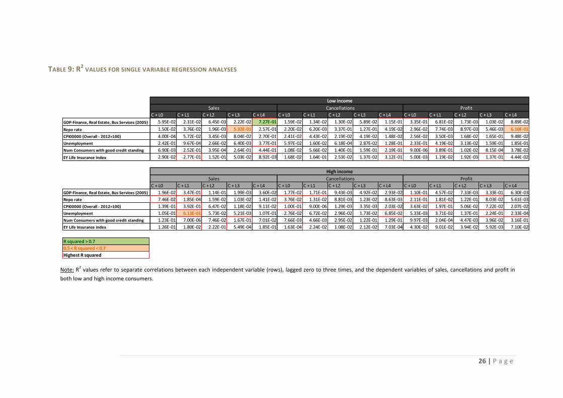
26 | P a g e
TABLE 9: R2 VALUES FOR SINGLE VARIABLE REGRESSION ANALYSES
Note: R2 values refer to separate correlations between each independent variable (rows), lagged zero to three times, and the dependent variables of sales, cancellations and profit in
both low and high income consumers.
C + L0 C + L1 C + L2 C + L3 C + L4 C + L0 C + L1 C + L2 C + L3 C + L4 C + L0 C + L1 C + L2 C + L3 C + L4
GDP-Finance, Real Estate, Bus Services (2005) 5.95E-02 2.31E-02 6.45E-03 2.22E-02 7.27E-01 1.59E-02 1.34E-02 1.30E-02 5.89E-02 1.15E-01 3.35E-01 6.81E-02 1.73E-03 1.03E-02 8.89E-02
Repo rate 1.50E-02 3.76E-02 1.96E-03 5.32E-01 2.57E-01 2.20E-02 6.20E-03 3.37E-01 1.27E-01 4.19E-02 2.96E-02 7.74E-03 8.97E-03 5.46E-03 6.10E-01
CPI00000 (Overall - 2012=100) 4.00E-04 5.72E-02 3.45E-03 8.04E-02 2.70E-01 2.41E-02 4.43E-02 2.19E-02 4.19E-02 1.48E-02 2.56E-02 3.50E-03 1.68E-02 1.65E-01 9.48E-02
Unemployment 2.42E-01 9.67E-04 2.66E-02 6.40E-03 3.77E-01 5.97E-02 1.60E-02 6.18E-04 2.87E-02 1.28E-01 2.33E-01 4.19E-02 3.13E-02 1.59E-01 1.85E-01
Num Consumers with good credit standing 6.90E-03 2.52E-01 3.95E-04 2.64E-01 4.44E-01 1.08E-02 5.66E-02 1.40E-01 1.59E-01 2.19E-01 9.00E-06 3.89E-01 1.02E-02 8.15E-04 3.78E-02
EY Life Insurance index 2.90E-02 2.77E-01 1.52E-01 5.03E-02 8.92E-03 1.68E-02 1.64E-01 2.53E-02 1.37E-02 3.12E-01 5.00E-03 1.19E-02 1.92E-03 1.37E-01 4.44E-02
C + L0 C + L1 C + L2 C + L3 C + L4 C + L0 C + L1 C + L2 C + L3 C + L4 C + L0 C + L1 C + L2 C + L3 C + L4
GDP-Finance, Real Estate, Bus Services (2005) 1.96E-02 3.47E-01 1.14E-01 1.99E-03 3.60E-02 1.77E-02 1.71E-01 9.43E-03 4.92E-02 2.93E-02 1.10E-01 4.57E-02 7.33E-03 3.33E-01 6.30E-03
Repo rate 7.46E-02 1.85E-04 1.59E-02 1.03E-02 1.41E-02 3.76E-02 1.31E-02 8.81E-03 1.23E-02 8.63E-03 2.11E-01 1.81E-02 1.22E-01 8.03E-02 5.61E-03
CPI00000 (Overall - 2012=100) 1.39E-01 3.92E-01 6.47E-02 1.18E-02 9.11E-02 1.00E-01 9.00E-06 1.29E-03 3.35E-03 2.03E-02 3.63E-02 1.97E-01 5.06E-02 7.22E-02 2.07E-02
Unemployment 1.05E-01 6.13E-01 5.73E-02 5.21E-03 1.07E-01 2.76E-02 6.72E-02 2.96E-02 1.73E-02 6.85E-02 5.33E-03 3.71E-02 1.37E-01 2.24E-01 2.33E-04
Num Consumers with good credit standing 1.23E-01 7.00E-06 7.46E-02 1.67E-01 7.01E-02 7.66E-03 4.66E-03 2.95E-02 1.22E-01 1.29E-01 9.97E-03 2.04E-04 4.47E-03 3.96E-02 3.16E-01
EY Life Insurance index 1.26E-01 1.80E-02 2.22E-01 5.49E-04 1.85E-01 1.63E-04 2.24E-02 1.08E-02 2.12E-02 7.03E-04 4.30E-02 9.01E-02 3.94E-02 5.92E-03 7.10E-02
Sales Cancellations Profit
Low income
Sales Cancellations Profit
High income
R squared > 0.7
0.5 < R squared < 0.7
Highest R squared
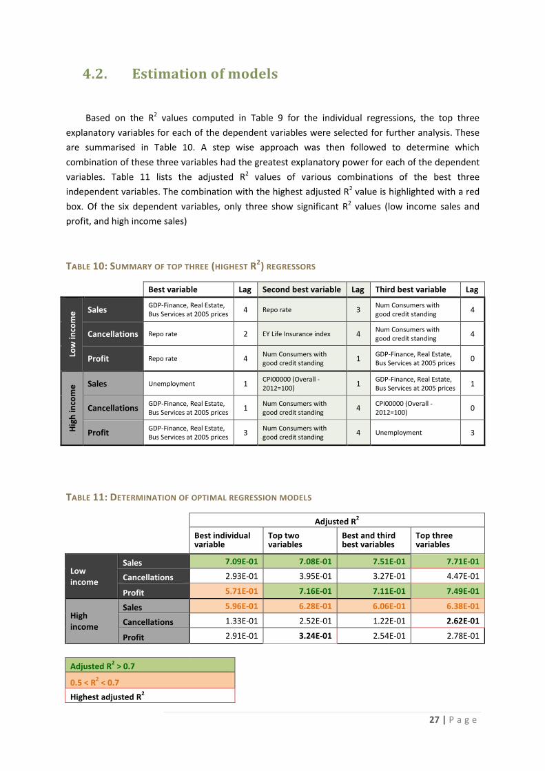
27 | P a g e
4.2. Estimation of models
Based on the R2 values computed in Table 9 for the individual regressions, the top three
explanatory variables for each of the dependent variables were selected for further analysis. These
are summarised in Table 10. A step wise approach was then followed to determine which
combination of these three variables had the greatest explanatory power for each of the dependent
variables. Table 11 lists the adjusted R2 values of various combinations of the best three
independent variables. The combination with the highest adjusted R2 value is highlighted with a red
box. Of the six dependent variables, only three show significant R2 values (low income sales and
profit, and high income sales)
TABLE 10: SUMMARY OF TOP THREE (HIGHEST R2) REGRESSORS
Best variable Lag Second best variable Lag Third best variable Lag
Low
inco
me
Sales GDP-Finance, Real Estate, Bus Services at 2005 prices
4 Repo rate 3 Num Consumers with good credit standing
4
Cancellations Repo rate 2 EY Life Insurance index 4 Num Consumers with good credit standing
4
Profit Repo rate 4 Num Consumers with good credit standing
1 GDP-Finance, Real Estate, Bus Services at 2005 prices
0
Hig
h in
com
e Sales Unemployment 1
CPI00000 (Overall - 2012=100)
1 GDP-Finance, Real Estate, Bus Services at 2005 prices
1
Cancellations GDP-Finance, Real Estate, Bus Services at 2005 prices
1 Num Consumers with good credit standing
4 CPI00000 (Overall - 2012=100)
0
Profit GDP-Finance, Real Estate, Bus Services at 2005 prices
3 Num Consumers with good credit standing
4 Unemployment 3
TABLE 11: DETERMINATION OF OPTIMAL REGRESSION MODELS
Adjusted R
2
Best individual variable
Top two variables
Best and third best variables
Top three variables
Low income
Sales 7.09E-01 7.08E-01 7.51E-01 7.71E-01
Cancellations 2.93E-01 3.95E-01 3.27E-01 4.47E-01
Profit 5.71E-01 7.16E-01 7.11E-01 7.49E-01
High income
Sales 5.96E-01 6.28E-01 6.06E-01 6.38E-01
Cancellations 1.33E-01 2.52E-01 1.22E-01 2.62E-01
Profit 2.91E-01 3.24E-01 2.54E-01 2.78E-01
Adjusted R2 > 0.7
0.5 < R2 < 0.7
Highest adjusted R2
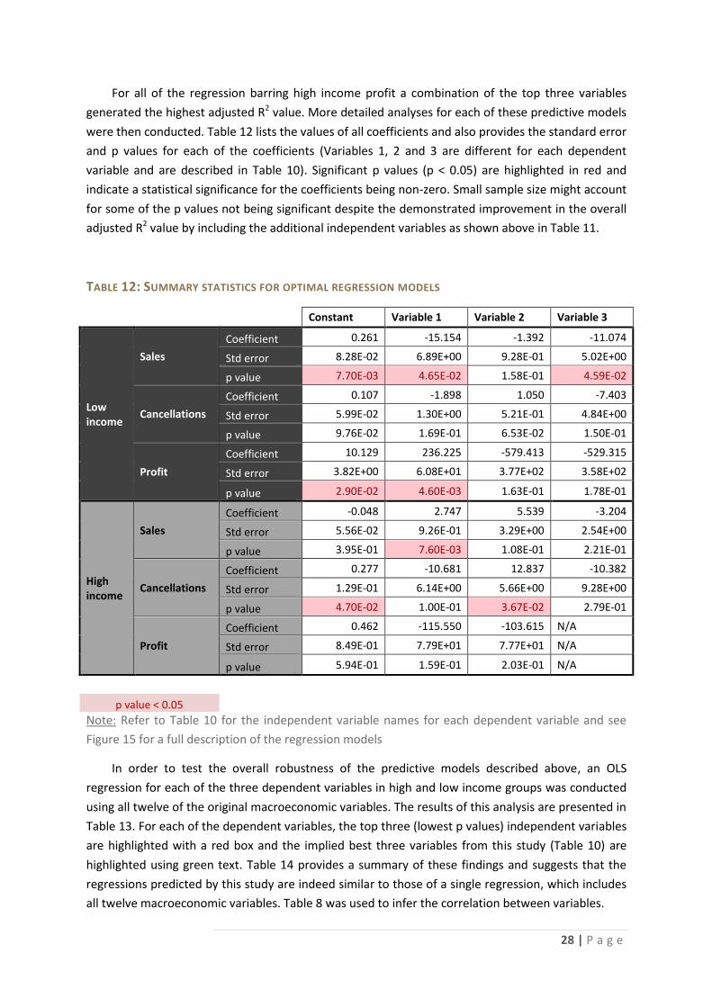
28 | P a g e
For all of the regression barring high income profit a combination of the top three variables
generated the highest adjusted R2 value. More detailed analyses for each of these predictive models
were then conducted. Table 12 lists the values of all coefficients and also provides the standard error
and p values for each of the coefficients (Variables 1, 2 and 3 are different for each dependent
variable and are described in Table 10). Significant p values (p < 0.05) are highlighted in red and
indicate a statistical significance for the coefficients being non-zero. Small sample size might account
for some of the p values not being significant despite the demonstrated improvement in the overall
adjusted R2 value by including the additional independent variables as shown above in Table 11.
TABLE 12: SUMMARY STATISTICS FOR OPTIMAL REGRESSION MODELS
Constant Variable 1 Variable 2 Variable 3
Low income
Sales
Coefficient 0.261 -15.154 -1.392 -11.074
Std error 8.28E-02 6.89E+00 9.28E-01 5.02E+00
p value 7.70E-03 4.65E-02 1.58E-01 4.59E-02
Cancellations
Coefficient 0.107 -1.898 1.050 -7.403
Std error 5.99E-02 1.30E+00 5.21E-01 4.84E+00
p value 9.76E-02 1.69E-01 6.53E-02 1.50E-01
Profit
Coefficient 10.129 236.225 -579.413 -529.315
Std error 3.82E+00 6.08E+01 3.77E+02 3.58E+02
p value 2.90E-02 4.60E-03 1.63E-01 1.78E-01
High income
Sales
Coefficient -0.048 2.747 5.539 -3.204
Std error 5.56E-02 9.26E-01 3.29E+00 2.54E+00
p value 3.95E-01 7.60E-03 1.08E-01 2.21E-01
Cancellations
Coefficient 0.277 -10.681 12.837 -10.382
Std error 1.29E-01 6.14E+00 5.66E+00 9.28E+00
p value 4.70E-02 1.00E-01 3.67E-02 2.79E-01
Profit
Coefficient 0.462 -115.550 -103.615 N/A
Std error 8.49E-01 7.79E+01 7.77E+01 N/A
p value 5.94E-01 1.59E-01 2.03E-01 N/A
p value < 0.05 Note: Refer to Table 10 for the independent variable names for each dependent variable and see
Figure 15 for a full description of the regression models
In order to test the overall robustness of the predictive models described above, an OLS
regression for each of the three dependent variables in high and low income groups was conducted
using all twelve of the original macroeconomic variables. The results of this analysis are presented in
Table 13. For each of the dependent variables, the top three (lowest p values) independent variables
are highlighted with a red box and the implied best three variables from this study (Table 10) are
highlighted using green text. Table 14 provides a summary of these findings and suggests that the
regressions predicted by this study are indeed similar to those of a single regression, which includes
all twelve macroeconomic variables. Table 8 was used to infer the correlation between variables.
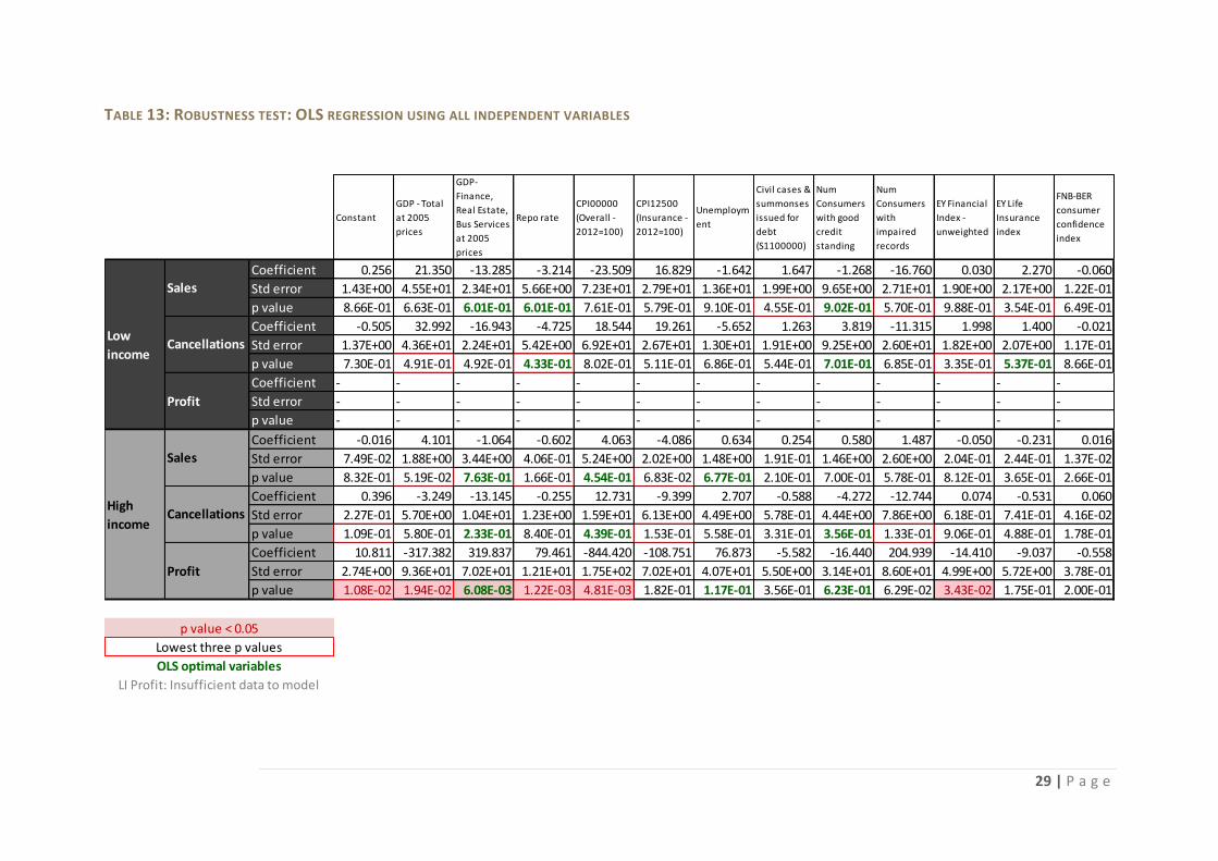
29 | P a g e
TABLE 13: ROBUSTNESS TEST: OLS REGRESSION USING ALL INDEPENDENT VARIABLES
Constant
GDP - Total
at 2005
prices
GDP-
Finance,
Real Estate,
Bus Services
at 2005
prices
Repo rate
CPI00000
(Overall -
2012=100)
CPI12500
(Insurance -
2012=100)
Unemploym
ent
Civil cases &
summonses
issued for
debt
(S1100000)
Num
Consumers
with good
credit
standing
Num
Consumers
with
impaired
records
EY Financial
Index -
unweighted
EY Life
Insurance
index
FNB-BER
consumer
confidence
index
Coefficient 0.256 21.350 -13.285 -3.214 -23.509 16.829 -1.642 1.647 -1.268 -16.760 0.030 2.270 -0.060
Std error 1.43E+00 4.55E+01 2.34E+01 5.66E+00 7.23E+01 2.79E+01 1.36E+01 1.99E+00 9.65E+00 2.71E+01 1.90E+00 2.17E+00 1.22E-01
p value 8.66E-01 6.63E-01 6.01E-01 6.01E-01 7.61E-01 5.79E-01 9.10E-01 4.55E-01 9.02E-01 5.70E-01 9.88E-01 3.54E-01 6.49E-01
Coefficient -0.505 32.992 -16.943 -4.725 18.544 19.261 -5.652 1.263 3.819 -11.315 1.998 1.400 -0.021
Std error 1.37E+00 4.36E+01 2.24E+01 5.42E+00 6.92E+01 2.67E+01 1.30E+01 1.91E+00 9.25E+00 2.60E+01 1.82E+00 2.07E+00 1.17E-01
p value 7.30E-01 4.91E-01 4.92E-01 4.33E-01 8.02E-01 5.11E-01 6.86E-01 5.44E-01 7.01E-01 6.85E-01 3.35E-01 5.37E-01 8.66E-01
Coefficient - - - - - - - - - - - - -
Std error - - - - - - - - - - - - -
p value - - - - - - - - - - - - -
Coefficient -0.016 4.101 -1.064 -0.602 4.063 -4.086 0.634 0.254 0.580 1.487 -0.050 -0.231 0.016
Std error 7.49E-02 1.88E+00 3.44E+00 4.06E-01 5.24E+00 2.02E+00 1.48E+00 1.91E-01 1.46E+00 2.60E+00 2.04E-01 2.44E-01 1.37E-02
p value 8.32E-01 5.19E-02 7.63E-01 1.66E-01 4.54E-01 6.83E-02 6.77E-01 2.10E-01 7.00E-01 5.78E-01 8.12E-01 3.65E-01 2.66E-01
Coefficient 0.396 -3.249 -13.145 -0.255 12.731 -9.399 2.707 -0.588 -4.272 -12.744 0.074 -0.531 0.060
Std error 2.27E-01 5.70E+00 1.04E+01 1.23E+00 1.59E+01 6.13E+00 4.49E+00 5.78E-01 4.44E+00 7.86E+00 6.18E-01 7.41E-01 4.16E-02
p value 1.09E-01 5.80E-01 2.33E-01 8.40E-01 4.39E-01 1.53E-01 5.58E-01 3.31E-01 3.56E-01 1.33E-01 9.06E-01 4.88E-01 1.78E-01
Coefficient 10.811 -317.382 319.837 79.461 -844.420 -108.751 76.873 -5.582 -16.440 204.939 -14.410 -9.037 -0.558
Std error 2.74E+00 9.36E+01 7.02E+01 1.21E+01 1.75E+02 7.02E+01 4.07E+01 5.50E+00 3.14E+01 8.60E+01 4.99E+00 5.72E+00 3.78E-01
p value 1.08E-02 1.94E-02 6.08E-03 1.22E-03 4.81E-03 1.82E-01 1.17E-01 3.56E-01 6.23E-01 6.29E-02 3.43E-02 1.75E-01 2.00E-01
LI Profit: Insufficient data to model
Lowest three p values
p value < 0.05
OLS optimal variables
Low
income
Sales
Cancellations
Profit
High
income
Sales
Cancellations
Profit

30 | P a g e
TABLE 14: SUMMARY OF ROBUSTNESS TEST FOR REGRESSION MODELS
Variables predicted in study
Variables suggested by single regression
Discussion
Low
inco
me
Sales
GDP-Finance, Real Estate, Bus Services at 2005 prices Repo rate Num Consumers with good credit standing
Civil cases & summonses issued for debt (S1100000) EY Life Insurance index Num Consumers with impaired records
Two of the three independent variables suggested by the study overlap with variables estimated by the single regression. Only the Repo rate and EY Life insurance index are uncorrelated
Cancellations
Repo rate EY Life Insurance index Num Consumers with good credit standing
Repo rate EY Financial Index –unweighted GDP - Total at 2005 prices
The Repo rate is suggested in both regression analyses as are the slightly correlated EY indices. The two models differ in the selection of the third best variable
Profit
Repo rate Num Consumers with good credit standing GDP-Finance, Real Estate, Bus Services at 2005 prices
- Data set too small to conduct analysis
Hig
h in
com
e
Sales
Unemployment CPI00000 (Overall - 2012=100) GDP-Finance, Real Estate, Bus Services at 2005 prices
Repo rate CPI12500 (Insurance - 2012=100) GDP - Total at 2005 prices
Inflation (CPI) and GDP are suggested as explanatory variables in both regression analyses with unemployment being excluded from the single regression test case
Cancellations
GDP-Finance, Real Estate, Bus Services at 2005 prices Num Consumers with good credit standing CPI00000 (Overall - 2012=100)
Constant Num Consumers with impaired records CPI12500 (Insurance - 2012=100)
Credit worthiness and inflation (CPI) are suggested in both regressions as explanatory variables. In the single regression no other variables showed higher p values than the constant, but GDP was significant in the study
Profit
GDP-Finance, Real Estate, Bus Services at 2005 prices Num Consumers with good credit standing Unemployment
GDP-Finance, Real Estate, Bus Services at 2005 prices Repo CPI00000 (Overall - 2012=100)
All three variable suggested in this study were identified directly or through correlated variables in the single regression
Highly correlated or matching variables are highlighted in green Weakly correlated variables are highlighted in orange
This above robustness test provides strong support for the predictive models put forward in this
study. Finally, for each of the six proposed regression models (Table 12), a series of statistical
analyses were performed in order to test the assumptions of residual errors being i) normally
distributed, ii) homoscedastic and iii) not autocorrelated. These findings are summarised in Table 15.
Only the regressions for high income cancellations violated any assumptions (both normality and
homoscedasticity). Since this adjusted R2 value for this particular dependent variable was low
(0.262), this violation was not deemed important as the model itself is not highly predictive. Figure
14 shows graphical plots, where the actual values of the dependent variables are compared to the
predictive regression models.
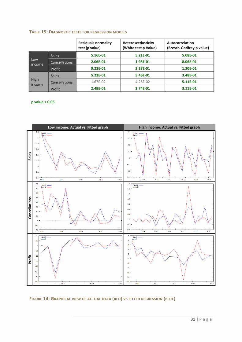
31 | P a g e
TABLE 15: DIAGNOSTIC TESTS FOR REGRESSION MODELS
Residuals normality test (p value)
Heteroscedasticity (White test p Value)
Autocorrelation (Bresch-Godfrey p value)
Low income
Sales 5.16E-01 5.21E-01 5.08E-01
Cancellations 2.06E-01 1.93E-01 8.06E-01
Profit 9.23E-01 2.27E-01 1.30E-01
High income
Sales 5.23E-01 5.46E-01 3.48E-01
Cancellations 1.67E-02 4.28E-02 5.11E-01
Profit 2.49E-01 2.74E-01 3.11E-01
p value > 0.05
Low income: Actual vs. Fitted graph High income: Actual vs. Fitted graph
Sale
s
Can
cella
tio
ns
Pro
fit
FIGURE 14: GRAPHICAL VIEW OF ACTUAL DATA (RED) VS FITTED REGRESSION (BLUE)

32 | P a g e
Figure 15 summarises the proposed regression models for each of the dependent variables.
Based on the adjusted R2 values (Table 11) only the models highlighted in red appear to have
significant explanatory power. The regressions for low income sales and profits had the highest
adjusted R2 values (0.77 and 0.75 respectively), while high income sales had an adjusted R2 value of
0.64. These three regression models thus serve as potentially strong predictors of sales and
profitability in the insurance industry. The models suggest that movements in GDP, consumer credit
standing and the repo rate will inform future sales and profitability for low income consumer groups;
while future sales in high income consumer groups are better explained by changes in
unemployment, CPI and GDP.
General equation: 𝐼𝑛𝑠𝑢𝑟𝑎𝑛𝑐𝑒 𝑑𝑒𝑚𝑎𝑛𝑑 = 𝛽0 + 𝛽1 𝑉1 + 𝛽2 𝑉2 + 𝛽3 𝑉3
Where 𝛽𝑖 are coefficients and 𝑉𝑖 are independent variables
Key to variable names:
CPI00000 (All - 2012=100) C
EY Life insurance index E
GDP-Finance, Real Estate, Business Services at 2005 prices G
Number of consumers with good credit standing N
Repo rate R Unemployment U
Low income: Sales = 0.261 - 15.154 G(L4) - 1.392R(L3) - 11.074 N(L4) Cancellations = 0.107 - 1.898R(L2) + 1.050 E(L4) - 7.403 N(L4) Profit = 10.129 + 236.225R(L4) - 579.413 N(L1) - 529.315 G(L0)
High income:
Sales = -0.048 + 2.747U(L1) + 5.539 C(L1) - 3.204 G(L1) Cancellations = 0.277 - 10.681 G(L1) + 12.837 N(L4) - 10.382 C(L0) Profit = 0.462 - 115.550 G(L3) - 103.615 N(L4)
Note: Equations in red have adjusted R2 values > 0.64 Subscripts explain the variable lags
FIGURE 15: PROPOSED REGRESSION MODELS

33 | P a g e
4.3. Interpretation of results and discussion
The objective of this research was to determine whether insurance demand can be explained by
any macroeconomic factors. Two sample cohorts were selected for this study; a low income group
and a high income group. The underlying hypothesis being that a low income consumer may be
more sensitive and responsive to shifts in the macroeconomic environment than a high income
consumer. This builds on early studies which modelled insurance demand (risk aversion) as a
function of wealth and net worth (Mossin, 1968; Pratt, 1964). Since net worth and risk aversion have
an inverse relationship, it is reasonable to propose that high income consumers’ demand for
insurance is not tightly coupled to the macro economy and rather based on individual demographic
factors such as age, education, family size, marital status, race, gender and religion (Liebenberg et
al., 2012; Zietz, 2003). In order to explore this, insurance demand and profitability were investigated
in this study using three different variables: sales, cancellations and underwriting profit.
Sales
Models with significant adjusted R2 values were identified for sales in both the low and high
income data sets. Interestingly, only GDP (Finance, Real Estate, and Business Services) was a
common independent variable for both models, but was most informative with four lags in the low
income group and only one lag in the high income group. The coefficient in both models was
negative, which suggests that as the macro economy contracts insurance demand increases. This
supports a view that consumer risk aversion is dynamic and seems to have an inverse relationship to
economic performance.
Sales to low income consumers also had an inverse relationship to the repo rate (three lags) and
their credit standing (four lags). As the repo rate increases prime interest rates tend to increase and
thus the cost of borrowing increases, which is likely to impact low income consumers and reduce
consumption. The negative coefficient for credit standing might imply that individuals with a
sustainable ability to support current consumption levels may change their risk aversion and start to
self-insure. All of the independent variables used to explain sales to low income consumers had 3 or
4 lags, which suggests a slow response time to macroeconomic factors.
Conversely all explanatory variables used for high income sales only had one lag. In addition to
GDP, sales to high income consumers showed proportional relationships to inflation (total CPI) and
unemployment. The positive coefficients for CPI and unemployment are of interest. In the case of
demand push inflation an inverse relationship is expected; however if cost push inflation occurs,
then inflation and unemployment can move together causing stagflation.
Generally, inflationary increases and higher unemployment lead to reduced consumption. In
this case high income consumers may actually be adjusting their consumption based on sentiment
and not financial constraint. The policies sold in this study are individual Life policies and the short
lags (quick response time) suggests that buying behaviours are proactive rather than reactive as is
34 | P a g e
the case for the low income consumers where macroeconomic changes take up to a year to start
affecting buying behaviours.
Cancellations
Neither low nor high income groups demonstrated any significant correlation between the
selected macroeconomic factors and policy cancellations. Policy sales were influenced by inflation,
interest rates, unemployment and credit standing; which ultimately relate to an individual’s net
worth. Although some of these variables produced the “best” model for cancellations, the overall
adjusted R2 values were relatively low to deem significant (0.45 and 0.26 respectively for low and
high income consumers). Thus the decision to cancel an insurance policy is likely to be informed by
other social or demographic factors over and above macroeconomic factors (Schwarcz, 2010).
Underwriting profit
Profitability was well described for the low income consumer group with an adjusted R2 value of
0.75. Interestingly the explanatory variables were the same as those that influenced sales, the only
difference being a positive coefficient for the repo rate in the regression for profit. This is easily
explained by the investment income returns that Life insurers earn by investing premiums. In high
interest environments the returns will improve and thus the overall profitability of the business
should also improve (Frey & Steinmann, 2012; Karl et al., 2010).
Interestingly there is a lag of a year before a change to interest rates influences underwriting
profitability; however the other explanatory variables of consumer credit standing and GDP
(Finance, Real Estate, and Business Services) have more immediate impacts (one and zero lags,
respectively). Although GDP and consumer credit standing were common variables that also
produced the “best” model for high income consumer underwriting profits, the adjusted R2 was
quite low (0.32).
35 | P a g e
5. Conclusion
Understanding the drivers of insurance demand is complicated by the variety of products sold,
consumer segments, distribution channels and business environments. This study aimed to remove
some of this complexity by focusing on one type of product (Life insurance policies sold to
individuals), separating low from high income consumers and exploring insurance demand in a single
business environment. Three potential measures of insurance demand were investigated: new
business sales, policy cancellations and underwriting profit. For each of these dependent variables
an initial universe of twelve macroeconomic variables was identified and each candidate explanatory
variable was evaluated using an ordinary least squares regression analysis. Using a step wise
approach optimal regressions for each of the three dependent variables (sales, cancellations and
profitability split into high and low income groups) were defined. Three of the six regressions
generated adjusted R2 values which implied the models were informative.
Sales for both low and high income consumers were defined with GDP (Finance, Real Estate,
and Business Services) being a common independent variable. Other explanatory variables included
repo rate and consumer credit standing (low income) and unemployment and total CPI (high
income). As described in Chapter 4, the variable lags for low income consumers suggested buying
behaviours shifted slowly (up to 1 year) in response to macroeconomic changes, while high income
consumer responses were more rapid (3 months). This might suggest that the drivers of a shift in
buying behaviour may differ between low and high income consumers. The rapid response of high
income consumers might imply consumption is based on sentiment and personal preferences rather
than financial constraint. However, the insignificance of the EY Life insurance index in these models
is surprising and could discount this view.
Since both low income and high income consumer groups buying behaviours could be
successfully modelled, the hypothesis that high income consumers are insensitive to macroeconomic
changes cannot be supported. However, based on the above findings the underlying basis for the
shift in consumption has not been adequately explained. It is still an open question whether reduced
disposable income in low income consumers and sentiment / demographic factors in high income
consumers are the true drivers of the shifts in consumption in these two groups. A more detailed
study with a larger sample and additional demographic data may resolve this question.
Underwriting profits in the low income consumer group could also be explained well by the
proposed regression model, which included GDP (Finance, Real Estate, and Business Services), repo
rate and consumer credit standing. The overlap of independent variables between sales and profits
for the low income consumer models is not surprising and it rather suggests a natural relationship
between the two. The only difference is the positive correlation between repo rate and profits,
while for sales it has an inverse relationship. It is likely that the correlation between investment
returns and interest rates accounts for the positive correlation with profits (Frey & Steinmann, 2012;
Karl et al., 2010).
Unfortunately the sample sizes used in this study were too small to permit inclusion of forecast
tests. In order to progress and advance this study, it is essential to test the current models using hold

36 | P a g e
out samples and ideally with data sets from multiple insurers. This would help to substantiate the
current findings and allow for the creation of more robust models. Additional demographic factors
such as age, education, family size, marital status, race, gender and religion (Liebenberg et al., 2012;
Zietz, 2003), should also be included in order to separate whether insurance demand differs
between low and high income consumers based on demographic characteristics as well as
macroeconomic factors. A further extension would be to explore insurance demand across multiple
products. This would help businesses in making strategic decisions on which products to sell, and
which consumer segments to target based on prevailing macroeconomic conditions.

37 | P a g e
6. References
Anderson, D. R., & Nevin, J. R. 1975. Determinants of Young Marrieds' Life Insurance Purchasing Behavior: An Empirical Investigation. Journal of Risk and Insurance, 42(3): 375-387.
Barksdale, S., & Lund, T. 2006. 10 Steps to Successful Strategic Planning: ASTD Press.
Brooks, C. 2014. Introductory econometrics for finance: Cambridge university press.
Burnett, J. T., & Palmer, B. A. 1984. Examining Life Insurance Ownership through Demographic and Psychographic Characteristics. Journal of Risk and Insurance, 51(3): 453-467.
Chui, A. C. W., & Kwok, C. C. Y. 2009. Cultural practices and life insurance consumption: An international analysis using GLOBE scores. Journal of Multinational Financial Management, 19(4): 273-290.
Clark, D., Kent, J., & Morgan, E. 2013. Dynamic policyholder behaviour and management actions survey report. Milliman Survey: 59.
Doherty, N. A., & Kang, H. B. 1988. Interest rates and insurance price cycles. Journal of Banking & Finance, 12(2): 199-214.
Eighty20. 2014. General Household Survey 2012 - Persons. http://www.eighty20.co.za/databases/.
Frey, A., & Steinmann, L. 2012. Facing the interest rate challenge. Swiss Re sigma(4): 40.
FSB. 2014. https://www.fsb.co.za/Departments/insurance/Pages/documents.aspx#.
GraphPad Software, I. 2014. http://graphpad.com/quickcalcs/Grubbs1.cfm.
GRETL. 2014. GRETL software http://gretl.sourceforge.net/, 2014 ed.
Gwatidzo, T., & Ojah, K. 2009. Corporate capital structure determinants : evidence for five African countries, Vol. 11: 1-23.
Inseta. 2014. http://www.inseta.org.za/.
Kalra, A., & Futterknecht, O. 2011. Insurance in emerging markets: growth drivers and profitability. Swiss Re sigma(5): 35.
Karl, K., Holzheu, T., & Laster, D. 2010. The impact of inflation on insurers. Swiss Re sigma(4): 31.
Kirova, M., & Steinmann, L. 2012. Understanding profitability in life insurance. Swiss Re sigma(1): 33.
Ladekarl, J., & Zervos, S. 2004. Housekeeping and plumbing: the investability of emerging markets. Emerging Markets Review, 5(3): 267-294.
Lee, C.-C., & Chiu, Y.-B. 2012. The impact of real income on insurance premiums: Evidence from panel data. International Review of Economics & Finance, 21(1): 246-260.
Lee, C.-C., Lee, C.-C., & Chiu, Y.-B. 2013. The link between life insurance activities and economic growth: Some new evidence. Journal of International Money and Finance, 32(0): 405-427.

38 | P a g e
Liebenberg, A. P., Carson, J. M., & Dumm, R. E. 2012. A Dynamic Analysis of the Demand for Life Insurance. Journal of Risk and Insurance, 79(3): 619-644.
Mark, T., Niraj, R., & Dawar, N. 2012. Uncovering Customer Profitability Segments for Business Customers. Journal of Business-to-Business Marketing, 19(1): 1-32.
Mossin, J. 1968. Aspects of Rational Insurance Purchasing. Journal of Political Economy, 76(4): 553.
Nattermann, P. M. 2000. Best practice ≠ Best strategy. McKinsey Quarterly(2): 22-31.
Pratt, J. W. 1964. Risk Aversion in the Small and in the Large. Econometrica (pre-1986), 32(1,2): 122.
Prince, J. D. 1904. The Code of Hammurabi. The American Journal of Theology, 8(3): 601-609.
Reinartz, W. J., & Kumar, V. 2000. On the profitability of long-life customers in a noncontractual setting: An empirical investigation and implications for marketing. Journal of Marketing, 64(4): 17-35.
Reinartz, W. J., & Kumar, V. 2003. The Impact of Customer Relationship Characteristics on Profitable Lifetime Duration. Journal of Marketing, 67(1): 77-99.
Schwarcz, D. 2010. Insurance Demand Anomalies and Regulation. Journal of Consumer Affairs, 44(3): 557-577.
StatsSA. 2014. http://beta2.statssa.gov.za/.
SwissRe. 2014. http://www.swissre.com/sigma/.
Vandermerwe, S. 2004. Breaking Through: Implementing Customer Focus in Enterprises. New York: Palgrave Macmillan.
Zietz, E. N. 2003. Perspectives: An Examination of the Demand for Life Insurance. Risk Management & Insurance Review, 6(2): 159-191.