Embed Size (px)
Citation preview
An Empirical Assessment of the Efficiency of Trading Halts
to Disseminate Price-Sensitive Information During the Opening
Hours of a Stock Exchange. The Case of Euronext Brussels
Peter-Jan Engelen University of Antwerp, Belgium
Abstract This paper examines the effect of temporarily suspending the trading of exchange-listed individual stocks. It evaluates whether regulatory authorities can successfully use the mechanism of trading halts in forcing companies to disclose new and material information to the capital market. In contrast to previous studies which mainly concentrate on North-American stock markets, this study utilises a data set comprising of firms listed on Euronext Brussels. The results show that suspension is indeed an effective means of disseminating new information. Stock prices adjust completely and instantaneously to the new information released during trading suspensions. We also observe a significant increase in trading volume after the reinstatement of trading. On the other hand, we do not find any increase in stock return volatility around trading suspensions. Overall, the results confirm the efficacy of trading suspensions in disseminating new information. JEL-Code: G10, G14, G18 Keywords: information dissemination, trading halt, trading suspension, market efficiency
0.Introduction
Do investors care about the quality of the financial markets in which they operate? Although
an affirmative answer seems obvious and natural, only recently the so-called law and finance
literature, which was initiated by the seminal papers of La Porta, Lopez-de-Silanes, Shleifer
and Vishny (1997, 1998), investigated the relationship between a country’s legal framework
and its financial development. The law and finance literature offers strong empirical evidence
on the importance of the legal environment (market integrity, investor protection) for the
development of these markets and economic growth. La Porta e.a. (1997) show that a good
legal environment expands the ability of companies to raise external finance through either
debt or equity. In its recent proposal of the Market Abuse Directive, the European
Commission as well stresses the importance of an adequate legal framework in order for
companies to raise capital1: “High growth entreprises depend on the efficiency and
transparency of financial markets in order to raise capital. Indeed, the smooth functioning of
financial markets and public confidence in them are prerequisites for sustained economic
1 European Commission, Explanatory Memorandum, Proposal for a Directive of the European Parliament and of the Council on Insider Dealing and Market Manipulation, 30 May 2001, COM(2001) 281 final.

2
growth and wealth.” The Forum of European Securities Commissions (FESCO)2 and the
Federation of European Stock Exchanges (FESE) subscribe to that statement as well (see
FESCO, 2000, 2001 and FESE, 2000, 2001).
Although FESE and the European Commission are both committed to highest levels of
market quality, they disagree on the implementation. The European Commission supports the
idea of a single central, administrative regulatory authority in each EU Member State, which
should be independent of the exchanges. Because many exchanges demutualised fully,
confess to a profit motive and have become listed companies themselves such as Stockholm,
Deutsche Börse, Euronext and LSE, the European Commission argues that such exchanges
cannot any longer be entrusted with regulation as they have a conflict of interest (Arlman,
2001a, 2001b). However, for a stock exchange to be successful in the long term, it must be
able to show that it runs a fair and honest market for all participants, otherwise investors will
avoid trading in such a market. Or as Arlman (2002) puts it: “Serving as a quality market is
their most important brand.” Instead of a central authority substituting the supervision of the
exchanges, FESE (2001) stresses the complementary role of the exchanges and their
experience and investment in detection and market surveillance.
As the European Commission defines market abuse as a situation in which investors “have
used information which is not publicly available to their own advantage”, the supervision of
ongoing disclosure obligations, particularly to the ad-hoc disclosure of price-sensitive news,
is of crucial importance in order to promote market integrity and market quality. In this
respect, FESE (2001) particularly stresses the need for market knowledge and proximity and
supports the allocation of regulatory powers ‘closer to the market’. The alleged benefits of
allocating the supervision to the exchange itself are: (a) familiarity with the trading system
and its screening and filtering algorithms, (b) closer contact with market participants and (c)
more timely actions when market irregularities are detected, all of which are crucial elements
for installing trading halts for disseminating price-sensitive news. This empirical study adds
to the above debate because it examines whether an exchange can add value by ensuring
market integrity. In particular, it evaluates the use of trading halts on Euronext Brussels3 to
disseminate price-sensitive information during the opening hours of the stock exchange. Put
2 Now called the Committee of European Securities Regulators (CESR). 3 Formerly known as the Brussels Stock Exchange (BXS). In 2000 BXS, Amsterdam (Amsterdam Exchanges) and Paris (ParisBourseSBF) merged to the form the single securities market Euronext.

3
differently, it evaluates whether a supervision ‘close to the market’ can maintain an orderly
market.
A trading suspension (also known as trading halt) represents a temporary interruption in
official trading of an individual stock on a stock exchange4. Authorities usually adopt this
regulatory measure to provide investors extra time to evaluate newly released information
about a specific company. It is especially used when there may have been a breach of
confidence in relation to inside information or market manipulation, in which case companies
are required to disclose additional information. Therefore, trading suspensions are said to be a
crucial regulatory and supervisory measure in order to maintain a fair and orderly market in
which “all investors should have simultaneous access on a timely basis to the information
they require to take their investment decisions (FESCO, 2001).”
The desirability of trading suspension is subject to debate among regulators, market
participants and academics. Proponents of trading suspension argue that it provides traders
extra time to evaluate newly released information so that no specific group of investors obtain
an unduly advantage in stock trading. They also argue that stock prices become more
informative, uncertainty is reduced and investors are protected from volatile price movements.
On the other hand, critics argue that trading suspension simply delays stock price adjustments,
imposes additional costs to investors who are deprived of trading opportunities and makes an
exchange less attractive to investors. Ultimately, it is the supervisory authority that needs “to
weigh the benefits of allowing continuous trading against the desirability of interposing
processes which afford market users the opportunity to reassess a changed situation and to
alter their orders accordingly5.”
4 The term ‘trading halt’ is often used to refer to different kinds of regulatory measures. First, it has to be distinguished from a circuit breaker which involves a market-wide halt of trading of all stocks because of the movement of prices (or volumes) beyond pre-set parameters in order to reduce market volatility (e.g. rule 80B of the NYSE). Besides market-wide circuit breakers, restrictions on daily price variations of individual financial instruments also exist, such as the static and dynamic volatility interruptions on Euronext (see rule 4404/1 Euronext Rule Book and Euronext Instruction nr.4-01, Euronext Cash Market Trading Manual, Notice nr.2001-3807, 29 October 2001 and 2001-3840, 30 October 2001). Second, it has to be distinguished from listing suspensions when the supervisory authority decides to suspend the listing of a particular financial instrument until the situation of non-compliance with the continuing obligations arising from a listing, has been remedied. Finally, delisting refers to the permanent cancellation of the listing. The terms ‘trading halt’ and ‘trading suspension’ will be used interchangeably throughout the remainder of this paper and refers to suspensions related to the dissemination of price-sensitive information. 5 FESCO, Standards for Regulated Markets (99-FESCO-C), standard 7, paragraph 14.

4
This paper assesses the efficiency of trading halts to disseminate information among market
participants on Euronext Brussels. Therefore, we examine the pattern of trading activity
before and after the trading suspension in order to evaluate this regulatory policy measure.
Moreover, based on detailed information provided by the stock exchange, the empirical
analysis traces if the return behavior surrounding the trading halt is affected by the publicly
announced reason for the suspension. This is of major importance, because section one shows
that existing empirical studies mainly provide evidence for North-American stock markets,
while European stock markets are barely investigated with regard to the efficiency of trading
suspension. This current empirical research can therefore add new evidence with regard to the
use of a regulatory measure on small stock exchanges by examining trading suspensions on
Euronext Brussels. Moreover, examining Euronext Brussels offers an opportunity to evaluate
the efficiency of trading halts on a order-driven market with an electronic automated trading
system without any influence of market-makers or specialists on the effect of a trading
suspension, as is the case, for instance, on the New York Stock Exchange (NYSE). While
trading halts on the NYSE tend to protect specialists (Howe and Schlarbaum, 1986), trading
suspensions on Euronext Brussels don’t appear to protect any particular member or interest
group, but are intended to protect investors in general.
The remainder of this paper is organized as follows. In the next section, we review the
relevant literature. Section three explains the research design. It describes the data, the
sample, the variables and the methodology. Empirical results are reported in section four.
Conclusions and policy recommendations appear in the final section.
1.Review of Literature
Although several theoretical discussions on the use of a particular regulatory measure can be
made (see supra), the answer to the question on the efficiency of securities regulation is
mainly an empirical one. Several empirical studies investigated the suspension of trading of a
particular stock, mainly on North-American stock markets. However, the empirical results on
the efficiency of trading halts show mixed results.

5
Hopewell and Schwartz (1978) examine NYSE-initiated trading halts from 1974 till 1975.
News suspensions lasted for 261 minutes or approximately four and one-half hours6. Delayed
openings tended to last longer than intraday suspensions7 (437 minutes compared to 149
minutes). Securities experience a relatively large price adjustment during a trading halt, and
the longer the trading halt, the larger the price adjustment8. Their empirical results show that
security prices adjust rapidly to the new information released during the trading halt. Post-
trading halt abnormal return behavior shows that the price adjustment is almost complete by
the end of the trading halt. However, a commission-paying investor could not earn abnormal
trading profits. While prices react efficiently to significant new information, pre-trading halt
anticipatory price behavior can be detected. Although their analysis cannot distinguish
between the possible causes of this abnormal return behavior, Hopewell and Schwartz suggest
insider trading as a possible explanation. A distinction between bull and bear markets does
not result in different conclusions (Hopewell and Schwartz, 1976).
Apart from the stock exchanges, also the Securities and Exchange Commission (SEC) can
halt trading in U.S. markets. These trading suspensions are often intended to force compliance
with reporting and disclosure requirements to protect investors or to promote investor equity
by ensuring that sufficient information is available to make rational, informed decisions.
Compared to NYSE halts, SEC-initiated trading halts are less frequent (frequency of SEC-halt
is one tenth of NYSE-halts). The average length of the SEC-trading halts is substantially
longer: on average 12.2 weeks (Howe and Schlarbaum, 1986). It appears that SEC-trading
halts have to be viewed rather as a disciplinary measure to force compliance with securities
regulation. Howe and Schlarbaum find a substantial negative abnormal return over the trading
halt period. After the trading halt stock prices keep declining in the weeks thereafter.
Apparently, SEC-trading halts disclose unfavorable news, to which investors react very
slowly. No anticipatory abnormal return behavior is found. The Ferris, Kumar and Wolfe
(1992) study, which examines 40 SEC-initiated trading halt during 1959 and 1987, detects
anticipatory price behavior as well as no complete price adjustment to new information
released during the trading halt, especially for the bad news subsample.
6 News suspensions are initiated by a pending or actual news announcement which is deemed to have a significant impact on the market price of a security. The NYSE has another event triggering a trading halt: a substantial imbalance of buy and sell orders and are requested by specialists. These trading halts are called imbalance suspensions. See Hopewell and Schwartz (1978) for more details. 7 Trading halts that are initiated sometime after the opening trade. 8 Similar results are being reported by Schwartz (1976).

6
Other empirical studies focusing on major stock exchanges are Kryzanowski (1978, 1979) on
Canadian stock exchanges and Kabir (1994) on the London Stock Exchange (LSE).
Kryzanowski (1978) reports abnormal returns in the presuspension period as well as in the
postsuspension period. He concludes that trading halts are not an effective mechanism to
detect the exploitation of private information nor to disclose price-sensitive information
during the suspension of trading. Examining a slightly different sample Kryzanowski (1979)
distinguishes between good and bad new information. Both subsamples shows abnormal
returns prior to the trading halts, but only the bad news subsample show abnormal negative
returns in the postsuspension period. Only the disclosure of favourable news appears to be
efficient. Examining the trading halts on the LSE, Kabir (1994) confirms the doubts on the
efficiency of this mechanism in disseminating price-sensitive information. Anticipatory price
behavior as well as abnormal returns in the month following the month of trading reinstalment
are reported.
Where as the efficiency of trading halts on large stock exchanges as the NYSE, the Montreal
Stock Exchange or the London Stock Exchange is doubtful, empirical results on smaller stock
exchanges seem more promising. Examining the trading halts on the Stockholm Stock
Exchange (Sweden) De Ridder (1990) concludes that this is an effective mechanism to
disseminate new information. No abnormal return behavior is detected in the postsuspension
period, so prices fully adjust over the trading halt period. Moreover, no anticipatory price
behavior is found during the presuspension period indicating that insiders did not benefit
systematically from their informational advantage. Analogous conclusions can be drawn
regarding to the trading halts on the Amsterdam Stock Exchange (the Netherlands). The
market authority of the Amsterdam Stock Exchange appears to be very efficient in utilizing
this regulatory mechanism in order to disclose new information. Kabir (1992) detects no
anticipation of any trading halt, nor any share price behavior in the postsuspension period
indicating a possibility of abnormal profit-making. Share prices fully incorporate the
information released during the trading halt. With regard to the Stock Exchange of Hong
Kong, Wu (1998) shows that there are no abnormal profits in the postsuspension period.
However, some anticipatory price behavior is detected.
While previous empirical studies focused on return behavior around trading halts recent
empirical studies also examine volume and volatility patterns around the suspension of
trading. Examining SEC-halts, Ferris, Kumer and Wolfe (1992) observe a higher stock return
7
volatility in the presuspension period as well as in the postsuspension period. Only several
months later a significant decline of volatility is detected indicating that trading halts are not
effective in immediately reducing return volatility. Analogous results are reported with regard
to volume: higher than normal volume in the presuspension as well as in the postsuspension
period. Only four weeks after the trading halt normal volume patterns reoccur. Also Kabir
(1992) reports higher trading volume around trading halts on the Amsterdam Stock Exchange.
In his study, trading volume is slightly higher than normal in the ten-day period before the
trading halt, and significantly higher in the ten-day period after the suspension. Lee, Ready
and Seguin (1994) report increased volume and volatility after the reinstalment of trading on
the NYSE. Similar results are reported by Wu (1998) with regard to the Stock Exchange of
Hong Kong. Kryzanowski and Nemiroff (1998) detect higher trading activity in the
presuspension period on the Montreal Stock Exchange. Trading activity declines in the
postsuspension period, but is still higher than in the period prior to the event window. Also
increased volatility is reported in the presuspension and in the postsuspension period, but
volatility only increases temporarily in the postsuspension period and decreases within five
hours after the trading halt to its level of the pre-event window9.
This review of literature showed mixed results concerning the use of trading halts to
disseminate information among market participants. The efficiency of this regulatory measure
is doubtful on major stock markets as the NYSE, the Canadian market and the London Stock
Exchange. The efficiency on smaller stock markets as Stockholm or Amsterdam is more
promising. The remainder of this chapter analyzes whether the efficiency of trading
suspensions on Euronext Brussels is high or low and whether these results confirm the
empirical findings on the use of trading halts on small stock exchanges. Table 1 summarizes
the review of literature.
9 Given the existence of specialists on the NYSE or the Montreal Stock Exchange, some empirical studies focus on the role of specialists around trading halts. Because the role of specialist is irrelevant to this empirical study on the Brussels Stock Exchange, it will not be explained in extenso. See for details King, Pownall and Waymire (1991) and Kryzanowski and Nemiroff (1998). These studies focus on the price discovery process during trading halts using specialist indications (sequential forecasts of the upper and lower bounds of the security’s price at the resumption of trade). See King, Pownall and Waymire (1991, 518) for an example.

8
Table 1. Overview of the empirical studies on trading halts Study Country Final
sample of news
suspensions
Period examined in study
Who initiated the
trading halt?
Anticipatory price
behaviour?
Complete adjustment to
new information released during
trading halt?
Volume? Volatility?
Schwartz (1976) USA 242 Febr.’74 –Oct’74 NYSEa - - - - Hopewell and Schwartz (1976) USA Bull: 201
Bear: 300 Febr’74 – June‘75 NYSE yes yes - -
Hopewell and Schwartz (1978) USA 501 Febr’74 – June‘75 NYSE yes yes - - Kryzanowski (1978) Canada 34 Jan’67 –Dec’73 4 stock
exchanges yes no - -
Kryzanowski (1979) Canada Good: 43 Bad: 77
Jan’67 –Dec’73 4 stock exchanges
yes yes – good news no – bad news
- -
Howe and Schlarbaum (1986) USA 49 Febr’59 – May‘79 SEC no no - - De Ridder (1990) Sweden 137 Jan’80 – June‘88 SSE no yes - - Kabir (1992) Netherlands 59 Jan’83 – March’89 ASE no yes Increases - Ferris, Kumer and Wolfe (1992) USA 40 Febr’59 – Oct’87 SEC yes no Increases Increases Kabir (1994) UK 83 Jan’70 – March’88 LSE yes no - - Lee, Ready and Seguin (1994) USA 518 ‘88 NYSE - no Increases after
trading halt Increases after
trading halt Wu (1998) Hong-Kong 522 April’86-Dec.’93 SEHK yes yes Increases Increases Kryzanowski and Nemiroff (1998)
Canada 412 March-Aug’88 May-Oct’89
Oct’90-March’91
MSE - yes Increases Increases temporarily
a NYSE: New York Stock Exchange; SEC: Securities and Exchange Commission; SSE: Sweden Stock Exchange; ASE: Amsterdam Stock Exchange; LSE: London Stock Exchange; MSE: Montreal Stock Exchange; SEHK: Stock Exchange of Hong Kong

9
2.Research Design
2.1.Data
The initial population consisted of all suspensions of common stocks of Belgian companies
on Euronext Brussels from January 1992 through June 2000. This list totalled 210 trading
halts. This means, on average, 2.06 trading halts per month and 0.10 trading halts per trading
day or one trading halt every 10.1 trading days10. This list was provided by the Market
Authority of Euronext Brussels. The list included for each trading halt: the company name,
the date of the trading halt, the date of trading reinstatement, the last stock price before and
the first stock price after the trading halt and finally, the detailed reason for suspending the
trading11. When data was missing or was incomplete, additional data was collected from the
leading Belgian financial newspaper De Financieel Economische Tijd. Share price data were
collected from Datastream.
2.2.Sample description
The initial sample consisting of 210 trading halts was further reduced in several ways. First,
12 trading halts were deleted because these companies were delisted shortly after the
suspension of trading, meaning no after-suspension market price of the stock was formed.
These trading halts were mainly the result of a bankruptcy, a corporate reorganization ordered
by court or a regulatory measure of the supervisory authorities for non-compliance of the
disclosure regulation. Second, all related trading halts are left out of the sample. When the
trading is suspended in one stock, trading in related companies is suspended as well. For
example, when trading in Petrofina was suspended on 30 November 1998 because of the
takeover bid by Total, trading in the stocks of the shareholders of Petrofina was suspended as
well. In this way, seven other stocks were suspended: Tractebel, Electrabel, Sofina, NPM,
Sidro, GBL and Electrafina. Therefore the trading halts of related companies are left out of
the final sample. Thirdly, 31 observations were lost because of lack of data. These 31 trading
halts include mainly very small, thinly traded companies for which no stock price data was
available, such as Musson-Halanzy, Aiseau-Presle, Charbonnages du Hasard, Aurex or
Roumanie-Société Générale des Sucreries. Finally, 22 observations were excluded because of
10 Given 250 trading days in one year. 11 The author thanks Mr. V. Van Dessel and Mr. L. Delboo of Euronext Brussels for providing this data.

10
overlapping event periods as well as overlapping pre-event periods used for the estimation of
parameters to calculate abnormal returns (see infra). For instance, Ion Beam Applications
(IBA) was suspended on 15 February 1999 and again on 3 March 1999. Because the pre-event
period of the second trading halt includes the first trading halt, the estimation of the
parameters can be affected. Therefore, the second trading halt was left out of the sample.
In this way, the final sample consists out of 102 trading halts involving 72 companies. Of
these companies, 48 (66.67%) were suspended only once during the sample period, while 24
companies were suspended more than once. Eighteen companies were suspended two times
and six companies three times (see panel B in table 2). The average number of trading halts
per company is 1.42 and the median is 1.00 (see panel A in table 2). Of the 102 trading halts
from January 1992 through June 2000, 82 are single day suspensions (80.4%), while 20 are
multiday suspensions (19.6%). The average suspension period is 2.34 days (see panel A of
table 3). Panel B shows that 92% of all trading halts lasts two days or less.
Table 2.Number of trading halts per company for the final sample
Panel A. Number of trading halts
Number of trading halts 102
Number of companies 72
Average number of trading halts per company 1.42
Median number of trading halts per company 1.00
Panel B. Distribution over number of trading halts per company
Number of trading halts Number of companies 1 48 2 18 3 6 4 0 5 0
Table 3. Single day versus multiday trading halts of the final sample Panel A. Single versus multiday suspensions
single day 82 80.4% multiday 20 19.6% average 2.34 min 1 median 1 max 65
Panel B. Duration of suspension (number of days) 1 82 80.39% 2 12 11.76% 3 4 3.92% ≥4 4 3.92%
Legend: Final sample of 102 trading halts from January 1992 through June 2000

11
Table 4 give more descriptive statistics for the final sample of 102 trading halts. Panel A
through C give the distribution of the trading halts per year, per month and per day of the
week. Except for 1997, we notice that the number of trading halts increased substantially
during the last five years. There is no specific pattern of trading halts throughout the year.
Most trading halts occur in October, September and May, while the least trading halts occur
in August and June. Although most of the trading halts occur on Thursday, no day-of-the-
week pattern is present.
Table 4. Descriptive statistics for the final sample Absolute number Percentage
Panel A. Number of trading halts per year 1992 15 14.7% 1993 9 8.8% 1994 5 4.9% 1995 5 4.9% 1996 19 18.6% 1997 8 7.8% 1998 14 13.7% 1999 18 17.6% 2000 9 8.8%
Panel B. Number of trading halts per month
Jan 8 7.8% Febr 7 6.9% March 9 8.8% April 8 7.8% May 10 9.8% June 3 2.9% July 7 6.9% Aug 6 5.9% Sept 11 10.8% Oct 16 15.7% Nov 9 8.8% Dec 8 7.8%
Panel C. Number of trading halts per day of the week
Monday 18 17.6% Tuesday 13 12.7% Wednesday 21 20.6% Thursday 30 29.4% Friday 20 19.6%
Legend: Final sample of 102 trading halts from January 1992 through June 2000
Because the list provided by the Market Authority of Euronext Brussels included detailed
information on the reason for suspending the trading of each particular stock, each trading
halt of the final sample was categorized according to a specific type of news. A detailed list of
12
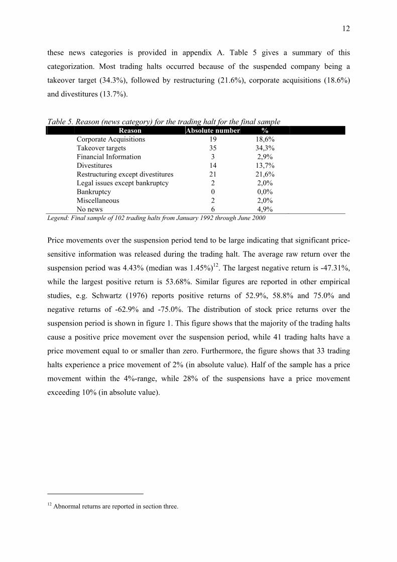
these news categories is provided in appendix A. Table 5 gives a summary of this
categorization. Most trading halts occurred because of the suspended company being a
takeover target (34.3%), followed by restructuring (21.6%), corporate acquisitions (18.6%)
and divestitures (13.7%).
Table 5. Reason (news category) for the trading halt for the final sample Reason Absolute number %
Corporate Acquisitions 19 18,6% Takeover targets 35 34,3% Financial Information 3 2,9% Divestitures 14 13,7% Restructuring except divestitures 21 21,6% Legal issues except bankruptcy 2 2,0% Bankruptcy 0 0,0% Miscellaneous 2 2,0% No news 6 4,9% Legend: Final sample of 102 trading halts from January 1992 through June 2000
Price movements over the suspension period tend to be large indicating that significant price-
sensitive information was released during the trading halt. The average raw return over the
suspension period was 4.43% (median was 1.45%)12. The largest negative return is -47.31%,
while the largest positive return is 53.68%. Similar figures are reported in other empirical
studies, e.g. Schwartz (1976) reports positive returns of 52.9%, 58.8% and 75.0% and
negative returns of -62.9% and -75.0%. The distribution of stock price returns over the
suspension period is shown in figure 1. This figure shows that the majority of the trading halts
cause a positive price movement over the suspension period, while 41 trading halts have a
price movement equal to or smaller than zero. Furthermore, the figure shows that 33 trading
halts experience a price movement of 2% (in absolute value). Half of the sample has a price
movement within the 4%-range, while 28% of the suspensions have a price movement
exceeding 10% (in absolute value).
12 Abnormal returns are reported in section three.

13
Figure 1.Frequency distribution of the average raw return over the suspension period for the final sample of 102 trading halts
0
2
4
6
8
10
12
14
16
18
20<-
0,40
-0,4
0<-0
,30
-0,3
0<-0
,20
-0,2
0<-0
,15
-0,1
5<-0
,10
-0,1
0<-0
,08
-0,0
8<-0
,06
-0,0
6<-0
,04
-0,0
4<-0
,02
-0,0
2<0,
00
>0,0
0-0,
02
>0,0
2-0,
04
>0,0
4-0,
06
>0,0
6-0,
08
>0,0
8-0,
10
>0,1
0-0,
15
>0,1
5-0,
20
>0,2
0-0,
30
>0,3
0-0,
40
>0,4
0
Return over suspension period
Num
ber o
f obs
erva
tions
2.3.Description of the variables
In the rest of this paper the following terms are used:
Ri, t = the logarithmic return of stock i in period t13
Rm, t = the logarithmic market index return in period t
ARi, t = abnormal return of stock i on day t of the estimation period
ARi, E = abnormal return of stock i on the event day
Rm, t = market index return on day t of the estimation period
Rm, E = market index return on the event day
mR = average market index return during the estimation period
N = number of stocks in the sample
T = number of trading days in the estimation period
is = estimated standard deviation of the abnormal return of stock i during the estimation
period
SARi, E = standardized abnormal return of stock i on the event day
w = number of stocks in the sample with a positive abnormal return on the event date

14
2.4.Methodology
To evaluate the efficiency of using trading halts to disseminate price-sensitive information
among market participants, an event-time study is used to analyze the impact of the trading
suspension. In this case the event is the suspension of the stock and therefore day 0 is defined
as the day on which the trading halt occurs, while day –1 is the trading day immediately
before the suspension day and day +1 is the day immediately after the suspension day. The
return on day 0 is calculated between the last closing price before the trading halt to the first
closing price after the trading halt, while the return of day +1 is calculated as the return
between this first closing price and the next day’s closing price14. While 80% of the trading
halts are single day suspensions (see table 2), 20 trading halts out of 102 are multiday
suspensions. In order to obtain comparable daily returns on event day 0, the multiday returns
over the suspension period are scaled by the number of suspension days.
An event study examines if the average abnormal return on the event day is equal to zero (null
hypothesis) versus an alternative hypothesis of a non-zero abnormal return:
≠=
0:0:
1
0
E
E
AARHAARH
[1]
The average abnormal return (AARE) on the event day is the aggregation of the individual
stock abnormal returns aligned in event time:
∑=
=N
iEiE AR
NAAR
1,
1 [2]
On the event day and on twenty trading days before and after the suspension, resulting in a
41-day event window15, abnormal returns are being calculated to examine returns behavior
around the trading halt. Individual stock abnormal returns are measured as the difference
between the realized or actual return on the event day (Ri, t) and the expected return E[Ri, t],
which is the benchmark normal return in the absence of the event:
13 The logarithmic return of a stock is calculated as:
+=
−1,
,,, ln
ti
tititi P
DPR , where Pi, t is the i-stock closing price
on trading day t, Di, t is the cash dividend paid on trading day t and Pi, t-1 is the i-stock closing price on trading day t-1, all adjusted for all capital changes as stock splits and stock dividends. 14 Although more precise data on raw returns is available, i.c. the return between the last market price before the trading halt and the first market price after the trading halt, the corresponding data on market index returns lacked. Therefore, returns on day 0 are calculated from close to close. 15 The typical length of the event period ranges from 21 to 121 days for daily studies. See Peterson (1989).

15
[ ]tititi RERAR ,,, −= [3]
Several methods exist to estimate the expected return of the stocks. In this study the market
adjusted model and the market model are used. Moreover, the market model is adjusted to
incorporate thin trading problems by using the Dimson (1979) methodology. These models
are discussed in the next section.
2.4.1.Calculating the benchmark expected return
The benchmark expected return for each individual stock depends on the model used:
[ ] tmti RRE ,, = , for the market-adjusted model,
[ ] tmiiti RbaRE ,,ˆˆ ⋅+= , for the market model,
[ ] tmDi
Diti RRE ,,
ˆˆ ⋅+= βα , for the Dimson model, and
The expected return of a stock in the market-adjusted model is the current market index
return. The market-adjusted abnormal return is thus equal to:
tmtiti RRAR ,,, −= [4]
This model uses no information from outside the event window to calculate abnormal returns
during the event period.
Market model abnormal returns are calculated as:
( )tmiititi RbaRAR ,,,ˆˆ ⋅+−= [5]
where ‘^’ denotes the OLS-estimates from the market model:
titmiiti eRbaR ,,, +⋅+= [6]
with
Ri, t = the return of stock i in period t
Rm, t = the market index return in period t
ai, bi = intercept and slope coefficient of the market model (stock-i-specific and time-
independent parameters)
ei, t = random disturbance term of the market model for stock i in period t

16
In order to calculate market model abnormal returns information from outside the event
window is used. The parameters of the market model are estimated over a period from –21 to
–140 trading days before the event day16.
When there is thin trading of stocks, the OLS-estimates of market model betas can be
affected. Thin trading of stocks can reduce the measured correlation with the market index,
and consequently the beta estimate: thinly traded stocks appear to have downward biased
betas, while actively traded stocks have upward biased beta estimates. These biased beta
estimates can cause biased abnormal returns and misspecified test statistics in event studies
(Strong, 1992). Our sample consists of many thinly traded stocks. Therefore, the Dimson
(1979)-method was used to adjust betas for the extent of thin trading17.
The estimation of the Dimson-beta consists of the aggregation of five estimated beta
coefficients using two lead and two lag variables18:
∑+=
−=
=2
2,
ˆˆk
kik
Di bβ , or [7]
iiiiiDi bbbbb ,2,1,0,1,2
ˆˆˆˆˆˆ++−− ++++=β [8]
The variables ikb ,ˆ with k = -2, -1, 0, +1, +2 are estimates of the slope coefficients in a multiple
regression of the stock return in period t against the return on the market in periods t-2, t-1, 0,
t+1 and t+2 (Dimson, 1979):
titmitmitmitmitmiiti wRbRbRbRbRbaR ,2,,21,,1,,01,,12,,2, +⋅+⋅+⋅+⋅+⋅+= ++++−−−− [9]
While the OLS-estimation of beta uses the complete (-140,-21) estimation-window, the
Dimson estimation uses an (-138,-23) estimation-window to allow for the two day leading and
lagging. The abnormal returns are calculated as (Brown and Warner, 1985):
tmDi
Dititi RRAR ,,,
ˆˆ ⋅−−= βα [10]
with
∑+=
−=
=2
2,
ˆˆk
kik
Di bβ , and [11]
16 The typical length of the estimation period ranges from 100 to 300 days for daily studies. See Peterson (1989). 17 An alternative procedure is Scholes and Williams (1977). However, Fowler and Rorke (1983) show that the choice between Dimson and Scholes-Williams is equivalent. 18 Empirical studies use a large variety of leads and lags. For instance, Brown and Warner (1985) use k=-3,…,0,… ,+3; Dimson and Marsh (1986) use k=-1,…,0,…,+5; Kabir (1994) uses k=-3,…,0,+1; O’Hanlon and Steel (1997) use k=-1,0,+1 and Ibbotson, Kaplan and Peterson (1997) use k=-1,0.

17
∑∑−=
−=
−=
−=
−=23
138,
23
138, 116
1ˆ116
1ˆt
ttm
Di
t
tti
Di RR βα [12]
However, the use of procedures to correct for thin trading can be questioned. Brown and
Warner (1985) show that there is no evidence that these procedures improve the specification
or the power of the tests. Similar results were found by Dyckman, Philbrick and Stephan
(1984). These findings were also reported by Reinganum (1982), Theobald (1983) and Cowan
and Sergeant (1996)19. Strong (1992) points out that, although OLS beta estimates can bias
the abnormal returns for an individual stock, these biases may average out to zero in the
sample of the event study. Moreover, Bartholdy and Riding (1994) show that OLS even
outperforms the use of alternative methods of beta estimation.
2.4.2.Test statistics
The traditional test procedure assuming cross-sectional independence is the Patell (1976)-
test20. This test statistic standardizes the abnormal return for each stock by its standard
deviation. The resulting test statistic is given by equation [13]21.
( )1,0~
42
1
1,
N
TT
SARZ
N
i i
i
N
iEi
∑
∑
=
=
−−
= [13]
with
( )( )∑
−=
−=
−
−++
=
21
140
2,
2,
,,
11ˆt
tmtm
mEm
ii
EiEi
RR
RRT
s
ARSAR [14]
However, traditional test statistics assume stable variances, meaning that there is no change in
variance between the estimation period and the event period. Event-induced variance, on the
19 Strong (1992) reports similar results found by Gheyara and Boatsman (1980), Dodd and Warner (1983), Linn and McConnell (1983) and Dopuch et al. (1986). 20 Since the trading halts occur independent of each other and no event-date clustering is present, no correction for cross-sectional dependence is necessary. Moreover, Brown and Warner (1985) point out that dependence adjustment can be harmful compared to procedures which assume independence because tests assuming cross-sectional dependence are only half as powerful and usually not better specified than test assuming independence.

18
other hand, means that the variance during the event window exceeds the variance over the
estimation period (Seiler, 2000). If the variance is underestimated, traditional test statistics
will reject the null hypothesis too frequently, even when the average abnormal return is in fact
zero (Brown and Warner, 1985; Boehmer, Musumeci and Poulsen, 1991). Several studies
report indeed increases of the variance of returns when certain events occur. A parametric test
that incorporates event-induced variance is offered by Boehmer, Musumeci and Poulsen
(1991). This test improves the Patell-test by allowing the abnormal return variances to differ
between the event and the estimation periods. They show that even a very small increase in
variance is very problematic for the traditional tests. Their test statistic incorporates variance
information from the estimation as well as the event window (Boehmer, Musumeci and
Poulsen, 1991):
( )
( )1,0~
11
1
1
2
1
,,
1,
N
NSAR
SARNN
SARNZ
N
i
N
i
EiEi
N
iEi
∑ ∑
∑
= =
=
−
−
= [15]
with
( )( )∑
−=
−=
−
−++
=
21
140
2,
2,
,,
11ˆt
tmtm
mEm
ii
EiEi
RR
RRT
s
ARSAR [16]
The main disadvantage of parametric tests is that they are based on assumptions about the
probability distribution of returns. Non-parametric tests do not depend on the assumption of
normality. Because non-parametric tests do not use the return variance, these tests are more
appropriate in case of event-induced variance. Two parametric tests are generally used: the
sign test (see infra) and the rank test of Corrado (1989). Corrado (1989), Corrado and Zivney
(1992) and Campbell and Wasley (1993) show that the rank test performs better than the
traditional test statistics in case of event-induced variance. The rank test is given by equation
[17] (Corrado, 1989 and Corrado and Zivney, 1992):
( )( )1,0~
5.011
0, NS
U
NZ
N
i U
i∑=
−= [17]
with
21 See section 1.3 for a description of the variables.

19
( )∑ ∑+
−= =
−=
20
140
2
1, 5.01
1611
t
N
iti
tU
t
UN
S [18]
( )1,
, +=
i
titi M
KU [19]
with Ki,t = rank (ARi,t), Mi represents the number of non-missing abnormal returns for stock i
and Nt represents the number of nonmissing abnormal returns in the cross-section of N firms
on day t in event time.
Besides event-induced variances, thin trading is another crucial problem for the event study
test specification. Cowan and Sergeant (1996) point out that thinly traded stocks are
characterized by numerous zero and large non-zero returns, causing non-normal return
distributions. This causes traditional test statistics to be poorly specified (Campbell and
Wasley, 1993). Similar results are reported by Maynes and Rumsey (1993) showing that the
rank test is a good alternative for thinly traded stocks causing traditional tests to be
misspecified. Cowan (1992) reports departures from normality (right skewness) causing
parametric tests based on the normality assumption to be less well specified for Nasdaq stocks
as compared to NYSE and AMEX stocks. Moreover, the rank test is also misspecified for
Nasdaq stocks! However, the generalized sign test performs well for thinly traded stocks. The
generalized sign test by Cowan (1992) is given in equation [22].
( )( )
( )1,0~ˆ1ˆ
ˆN
ppnpnwZ−
−= [20]
where w represents the number of stocks in the sample with a positive abnormal return on the
event date, p represents the fraction of positive abnormal returns expected under the null
hypothesis, and
∑ ∑=
−=
−=
=N
i
t
ttiN
p1
21
140,120
11ˆ ϕ [21]
with ϕi,t = 1 when ARi,E > 0 and 0 otherwise22.
The poorly specification of the Patell-test is also confirmed by Cowan and Sergeant (1996).
Their simulations show that the best test for thinly traded stocks with no increase of the return
variance on the event date is either the rank or the generalized sign test. In case of an increase

20
of the return variance on the event date, results are less clear. For lower-tailed tests the
generalized sign test should be used. For upper-tailed tests the standardized cross-sectional
test of Boehmer, Musumeci and Poulsen (1991) can be used, but it is not very powerful and it
risks to be misspecified if the variance increase does not occur. An alternative is the
generalized sign test, but it is misspecified in a few thinly traded samples. Results are
summarized in table 6.
In the remainder of this paper we perform both parametric and non-parametric tests to
determine statistical significance. The traditional Patell t-test assuming cross-sectional
independence is performed first23. Next, we also use the generalised sign test of Cowan
(1992) as a non-parametric test to test statistical significance of abnormal returns24.
Table 6. Best replacement of the Patell-test in case of event-induced variance or thinly traded stocks
Tickly traded stocks Thinly traded stocks
No variance
increase on
event date
Patell-test
-Generalized sign test
-Rank test
Variance
increase on
event date
-Standardized cross-sectional test of
Boehmer, et al. (1991)
-Rank test of Corrado (1989)
-Generalized sign test of Cowan (1992)
Lower-tailed tests:
-Generalized sign test
Upper-tailed tests:
-Standardized cross-sectional test
-Generalized sign test
Sources: Corrado (1989), Corrado and Zivney (1992), Cowan (1992), Campbell and Wasley (1993), Maynes and Rumsey (1993), Cowan and Sergeant (1996), Seiler (2000).
22 The difference between the generalized sign test and the traditional sign test is the value of p under the null hypothesis. While the traditional sign test uses a value of 0.50, the generalized sign test uses the fraction of positive returns in the estimation period, measured across N stocks and T days as value for p. 23 See equation [13]. 24 See equation [20].

21
3.Empirical results
The empirical analysis of the efficiency of trading halts on Euronext Brussels starts with an
examination of the abnormal returns in section 3.1. This analysis is completed by an analysis
of the abnormal trading volume in section 3.2 and the volatility of the stock returns around the
suspension in section 3.3.
3.1.Analysis of abnormal returns
3.1.1.Complete sample
Because trading halts are a regulatory action designed to disseminate price-sensitive
information among market participants, this section examines the process of the price
adjustment to this new information before, during and after the suspension. Through an
analysis of the valuation effects of the suspensions we can evaluate the effectiveness of
trading halts as a regulatory measure. If Euronext Brussels were a semi-strong form
informationally efficient stock market, the stock price would adjust instantaneously to the
new information that was released during the trading halt. Moreover, semi-strong form
efficiency would imply that there isn’t any anticipatory price behavior in the presuspension
period, nor any significant abnormal return behavior in the postsuspension period. In this
section we examine (a) if trading halts are associated with an important release of
information, (b) if there is any unusual return behavior before the suspension and (c) if there
is a complete adjustment to new information released during the trading halt.
To examine the abnormal return behavior over the suspension period, a market adjusted
model was used as the benchmark expected return (see equation [4]). Table 7 contains the
results for the entire sample of 102 suspensions from 1992 through 2000. The mean abnormal
return over the suspension period amounts 3,31%. The cumulative abnormal returns are
visualized in figure 2.
In order to test whether the abnormal returns in the event window are significantly different
from zero, a non-parametric test was used. For, as explained in section 2.4.2, the traditional t-
test performs very poorly in case of thin trading or variance increase on event date. Because
the sample in this study contains a large amount of thinly traded stocks, a generalized sign test

22
(see equations [20]) is used to test statistical significance of the abnormal returns. The
traditional t-test is merely reported for the sake of completeness25.
Figure 2. Market adjusted mean CARs for the entire sample from 1992 to 2000
-0,0100
0,0000
0,0100
0,0200
0,0300
0,0400
0,0500
-20 -18 -16 -14 -12 -10 -8 -6 -4 -2 0 2 4 6 8 10 12 14 16 18 20
Event window
CA
R
CAR
Note: CAR = market adjusted cumulative mean abnormal returns Sample size: n=102 suspensions
Table 7 shows that only the abnormal return over the trading suspension (day [0]) is
significantly different from zero. It appears that there is no anticipatory price behavior in the
presuspension period. The CAR over the presuspension period [-20, -1] is 0.45%, although
insignificant. Although many previous studies show anticipatory price behavior prior to the
trading halt (see e.g. Hopewell and Schwartz, 1978; Kryzanowski, 1979 or Kabir, 1994), our
results are in line with the findings on other small stock exchanges as Stockholm (De Ridder,
1990) or Amsterdam (Kabir, 1992).
Once the trading suspension is over, share prices do not follow any particular pattern.
Although the CAR in figure 2 shows a downward trend after the reinstalment of trading, this
is not statistically significant. We can conclude that share prices instantaneously incorporate
25 However, the results of the t-test have to be interpreted with caution because under the conditions of this sample, the traditional t-test will reject the null hypothesis of a zero abnormal return too often while in reality there is no abnormal return present.

23
the new information released during the trading halt. Again, these results are in line with De
Ridder (1990) and Kabir (1992)26.
Table 7.Market adjusted mean abnormal returns and cumulative abnormal returns for the entire sample from 1992 to 2000
Market adjusted (n = 102)
AR CAR t-test p-value Z-value Gen.Sign Test
-20 -0,0017 -0,0017 -0,85 0,3977 -0,41
-15 -0,0020 -0,0032 -1,35 0,1796 -0,21
-10 0,0017 -0,0005 1,97 0,0516 -0,01
-5 0,0025 0,0045 1,66 0,0995 1,38
-4 -0,0019 0,0026 -1,19 0,2374 0,39
-3 -0,0004 0,0022 -0,09 0,9296 -0,21
-2 -0,0011 0,0011 0,81 0,4197 0,78
-1 0,0034 0,0045 1,25 0,2154 0,39
0 0,0331 0,0377 28,20** 0,0000 2,96*
1 -0,0012 0,0364 0,22 0,8265 -0,01
2 -0,0024 0,0341 -0,40 0,6918 0,19
3 0,0038 0,0379 2,30* 0,0235 1,38
4 -0,0010 0,0369 -0,64 0,5267 -1,40
5 -0,0013 0,0356 -0,38 0,7017 1,18
10 -0,0033 0,0276 -1,92 0,0572 -0,81
15 0,0017 0,0253 0,54 0,5871 -0,01
20 -0,0034 0,0132 -1,43 0,1555 -1,00
Note: AR = market adjusted mean abnormal return CAR = market adjusted cumulative mean abnormal returns Sample size: n=102 suspensions t-test and p-value: test statistics for traditional t-test Z-value: test statistic for generalized sign test ** denotes significant at the 1% level * denotes significant at the 5% level
26 See table 1 for an overview of the abnormal return behavior on US markets.

24
3.1.2.Robustness of the benchmark model
To examine the sensitivity of the above results to the choice of the benchmark model to
calculate the abnormal returns, the analysis was repeated for the market model and the
Dimson model. The parameters ( iα and iβ ) of the market model are calculated over the 120
days estimation period, starting with day [-140] through day [-21]. Similar to Brown and
Warner (1985) we excluded all observations that did not have at least 30 daily returns in the
estimation period. In this way, the sample size was reduced to 82 observations. Because our
sample contains many thinly traded stocks, the beta estimate of the market model will be
biased downward (see section 2.4.1). Therefore, we use the Dimson-method to correct for thin
trading, using two lead and two lag variables. Although the average beta obtained from the
Dimson method (0.61) is much higher than the average beta from the OLS-estimation (0.14) it
is still fairly low. The abnormal returns around the trading halts using the market model and
the Dimson model as the benchmark expected return, are reported in appendix B. The results
are similar to the results obtained from the market adjusted model. The mean abnormal return
on day [0] is 3,43% and 3,45% for the market model and the Dimson model, respectively,
compared to 3,31% using the market adjusted model. Again, the generalized sign test shows
no significant abnormal returns prior to or after the trading halt.
Because the results are largely insensitive to the choice of the benchmark model, we use the
market adjusted model as benchmark instead of the market model or the Dimson model in the
rest of the chapter. First of all, the use of the latter would reduce the sample size from 102 to
82 observations. Secondly, the correct estimation of betas of thinly traded stocks is rather
difficult. Thirdly, Fedenia, Hodder and Triantis (1994) show that the estimation of betas can
seriously be distorted on stock exchanges, as Euronext Brussels, that are characterized by the
presence of holding companies and equity cross-holdings.
3.1.3.Subsamples based on news categories
Because the results, as shown in figure 2 and table 7, include the entire sample, it is difficult
to interpret these price adjustments. Because the entire sample includes both positive and
negative news, as well as different news categories (e.g. corporate acquisitions, restructuring
or legal issues), aggregation across securities makes the results difficult to interpret because of

25
potential offsetting price impacts of the different subsamples. Therefore, we divide the total
sample of trading halts in three subsamples according to the reason for the suspension. The
first subsample contains 54 trading halts for news concerning corporate acquisitions and
takeover targets27. This subsample is labelled “mergers and acquisitions”. The second
subsample includes all trading halts with regard to divestitures, as the sale of business
segments, participations and spin-offs. This group includes 14 observations. Finally, a
subsample of 21 trading halts is used for news related to other restructurings28. Although a
finer partitioning of the data, according to the detailed scheme in appendix A, would be very
useful, it is not possible because of the small sample size.
Figure 3. Mean CARs for the three subsamples based on the reason for the suspension
-0,0800
-0,0600
-0,0400
-0,0200
0,0000
0,0200
0,0400
0,0600
0,0800
0,1000
0,1200
-20 -18 -16 -14 -12 -10 -8 -6 -4 -2 0 2 4 6 8 10 12 14 16 18 20
Event window
CA
R
M&A Divest. Restr.
Note: CAR = market adjusted cumulative mean abnormal returns Sample size: n=54 (Mergers and acquisitions), n=14 (Divestitures) and n=21 (Restructuring)
27 See appendix A for the different new categories. 28 News categories 41 to 45 in appendix A.

26
Table 8. Abnormal returns and cumulative abnormal returns over the event window for three subsamples
Mergers and acquisitions (n=54) Divestitures (n=14) Restructuring (n=21)
AR CAR t-test p-value Z-value AR CAR t-test p-value Z-value AR CAR t-test p-value Z-value
-20 0,0016 0,0016 0,24 0,81 0,72 -0,0017 -0,0017 -0,53 0,60 -0,78 -0,0065 -0,0065 -0,92 0,37 -0,83
-15 -0,0036 -0,0035 -1,62 0,11 -0,37 0,0018 0,0125 0,62 0,54 0,29 -0,0031 -0,0074 -1,30 0,21 -0,83
-10 0,0022 -0,0045 1,91 0,06 0,45 -0,0028 0,0082 -0,21 0,84 -1,31 0,0068 0,0071 1,58 0,13 0,48
-5 0,0015 0,0047 0,80 0,43 0,99 0,0050 0,0103 1,76 0,10 0,83 -0,0013 0,0139 0,72 0,48 -0,39
-4 0,0000 0,0047 -0,74 0,46 0,99 0,0008 0,0110 0,91 0,38 0,83 -0,0046 0,0094 -1,00 0,33 -0,83
-3 0,0026 0,0074 0,99 0,33 1,27 0,0012 0,0122 0,14 0,89 -0,78 -0,0052 0,0042 -1,00 0,33 -1,70
-2 0,0047 0,0120 0,93 0,35 0,72 -0,0061 0,0062 0,35 0,73 0,29 0,0002 0,0044 1,12 0,28 0,92
-1 0,0027 0,0148 0,76 0,45 -0,37 0,0054 0,0115 1,89 0,08 -0,78 0,0017 0,0061 1,20 0,24 0,92
0 0,0803 0,0951 39,75** 0,00 3,72** -0,0040 0,0075 3,24** 0,01 0,83 -0,0366 -0,0304 -1,69 0,11 0,48
1 -0,0048 0,0903 -1,84 0,07 0,17 0,0136 0,0211 2,59* 0,02 0,29 -0,0079 -0,0384 -0,30 0,77 -0,83
2 -0,0019 0,0884 -0,62 0,54 0,99 -0,0042 0,0169 -1,09 0,30 -1,31 -0,0039 -0,0423 -0,13 0,89 -0,39
3 0,0080 0,0964 3,41** 0,00 2,36* 0,0033 0,0202 -1,70 0,11 -0,24 -0,0145 -0,0568 -1,40 0,18 -1,26
4 0,0031 0,0995 0,34 0,73 0,45 -0,0029 0,0174 -0,71 0,49 -1,31 -0,0069 -0,0637 -1,93 0,07 -1,70
5 0,0011 0,1006 0,02 0,98 0,17 -0,0037 0,0137 -1,03 0,32 -0,24 0,0006 -0,0631 0,72 0,48 3,11*
10 -0,0056 0,0861 -2,00 0,05 -0,92 -0,0032 0,0195 -1,22 0,25 -1,31 0,0001 -0,0604 0,07 0,94 0,48
15 0,0014 0,0832 -0,13 0,90 -0,10 0,0002 0,0219 0,37 0,72 0,29 0,0077 -0,0403 0,87 0,39 0,48
20 -0,0039 0,0746 -1,59 0,12 -1,73 0,0010 0,0089 0,45 0,66 0,83 -0,0044 -0,0500 -1,12 0,28 -0,39
Legend: n= number of trading halts in the sample; AR = market adjusted mean abnormal return; CAR = market adjusted cumulative mean abnormal return; t-test & p-value= test statistic resp. p-value for the traditional t-test; Z-value= test-statistic for the generalized sign test; ** denotes significant at the 1% level and * denotes significant at the 5% level

27
The results for the three subsamples are reported in table 8. Figure 3 contains a graphic
representation of the CARs. None of the three subsamples shows any anticipatory price
behavior. It appears that there is not any information leakage to the market with regard to
mergers and acquisitions, divestitures or restructuring plans. Over the suspension period the
mean abnormal return of the mergers and acquisitions subsample is 8,03%, which is
significant at the 1% level. The mean abnormal return for the divestitures and restructuring
subsamples are –0,4% and –3,66% respectively, although not statistically significant. Notice
that figure 3 shows that the mergers and acquisitions subsample have, an average, a positive
price impact, while the restructuring subsample has a negative price impact. If one compares
figure 3 and figure 2, it is clear that the mergers and acquisitions subsample dominates the
results of the total sample. Similar findings are reported by De Ridder (1990) for the Swedish
stock market29. Furthermore, table 8 shows that there is no significant abnormal return
behavior after the reinstalment of trading. It appears that stock prices adjust completely to the
new information released during the trading suspension.
3.1.4.Price impact over the span of the suspension period
Regardless of the sign of the price movement (positive or negative), figure 4 represents the
magnitude of the abnormal returns over the event window [-20, +20]. It is clear that a trading
halt is associated with the release of important price-sensitive information, resulting in an
abnormal return over 8% (in absolute value) on day [0]. This is not surprisingly because the
trading halts on Euronext Brussels are generally associated with the release of nonroutine and
extremely price-sensitive information as mergers and acquisitions or restructurings. Routine
announcements of earnings or dividends are in general not released during a trading halt.
Only three cases out of the total sample of 102 trading halts concern the release of financial
information as earnings or dividend announcements. Similar results are reported by King,
Pownall and Waymire (1991) for the US: 79.3% of their sample is related to disclosures about
corporate takeovers and leveraged buyouts, which cannot be predicted by investors, but which
have large price impacts.
29 Compare figures 3 and 4 in De Ridder (1990). His subsample of mergers and acquisitions contains 70 trading halts out of a total sample of 137 observations.

28
Figure 4. Magnitude of the abnormal returns over the event window
0,0000
0,0100
0,0200
0,0300
0,0400
0,0500
0,0600
0,0700
0,0800
0,0900
-20 -18 -16 -14 -12 -10 -8 -6 -4 -2 0 2 4 6 8 10 12 14 16 18 20
Event window
Abs
olut
e va
lue
(AR
)
ABS(AR)
Note: ABS(AR) = absolute value of the market adjusted mean abnormal returns Sample size: n=89 (Mergers and acquisitions, divestitures and restructuring) Figure 5. Median CARs for the three subsamples based on the reason for the suspension
-0,03
-0,02
-0,01
0
0,01
0,02
0,03
0,04
-20 -18 -16 -14 -12 -10 -8 -6 -4 -2 0 2 4 6 8 10 12 14 16 18 20
Event w indow
Med
ian
CA
R
M&A Restr. Divest.
Note: median CAR = market adjusted cumulative median abnormal returns Sample size: n=54 (Mergers and acquisitions), n=14 (Divestitures) and n=21 (Restructuring)

29
3.1.5.The impact of outliers
To test the impact of outliers on the mean abnormal returns, median abnormal returns are
calculated as well. The median abnormal return for the three subsamples are 3.11%, 0.19%
and 0.16% for the mergers and acquisitions, divestitures and restructuring subsamples,
respectively. In general, the conclusions of the median abnormal return analysis are similar to
the mean abnormal returns. No anticipatory stock price behavior and complete price
adjustment over the trading suspension (see table 9 and figure 5).
Table 9.Median abnormal returns and cumulative abnormal returns over the event window for three subsamples
Mergers and acquisitions Divestitures Restructuring
AR p-value CAR AR p-value CAR AR p-value CAR
-20 0,0003 0,4207 0,0003 -0,0042 0,4263 -0,0042 -0,0030 0,1349 -0,0030
-15 -0,0003 0,2025 -0,0046 0,0005 0,6698 -0,0033 -0,0040 0,1491 -0,0018
-10 0,0000 0,5156 -0,0062 -0,0039 0,2412 -0,0021 0,0025 0,3377 0,0061
-5 0,0016 0,3263 -0,0035 0,0023 0,4631 -0,0024 -0,0001 0,9861 0,0117
-4 0,0015 0,7962 -0,0020 0,0025 0,7064 0,0001 -0,0001 0,4340 0,0116
-3 0,0014 0,2056 -0,0006 -0,0003 0,9749 -0,0002 -0,0048 0,0885 0,0068
-2 0,0003 0,3705 -0,0002 0,0001 0,9515 -0,0001 0,0013 0,8649 0,0081
-1 -0,0002 0,6512 -0,0005 -0,0059 0,8077 -0,0060 0,0022 0,4041 0,0103
0 0,0311** 0,0000 0,0306 0,0019 0,7609 -0,0041 0,0016 0,5315 0,0119
1 -0,0001 0,4409 0,0305 0,0006 0,5830 -0,0035 -0,0019 0,5663 0,0100
2 0,0005 0,7664 0,0310 -0,0036 0,0580 -0,0070 -0,0002 0,7281 0,0099
3 0,0050** 0,0053 0,0360 -0,0007 0,7775 -0,0078 -0,0021 0,1790 0,0078
4 0,0001 0,7962 0,0361 -0,0010 0,3151 -0,0088 -0,0050 0,2722 0,0028
5 -0,0001 0,8228 0,0360 -0,0018 0,3792 -0,0105 0,0034* 0,0290 0,0062
10 -0,0009 0,1643 0,0352 -0,0035 0,4263 -0,0097 0,0013 0,6091 0,0111
15 -0,0001 0,6920 0,0323 -0,0003 0,8260 -0,0139 0,0016 0,3133 0,0133
20 -0,0028* 0,0453 0,0285 0,0013 0,5830 -0,0214 -0,0003 0,3754 0,0115
Note: AR = market adjusted median abnormal return CAR = market adjusted cumulative median abnormal returns Sample size: n=54 (Mergers and acquisitions), n=14 (Divestitures) and n=21 (Restructuring) p-value: test statistics for the Wilcoxon signed rank test ** denotes significant at the 1% level * denotes significant at the 5% level

30
3.1.6.Good news versus bad news subsamples
Besides subsamples based on the news categories of appendix A, another two subsamples are
formed: a good news and a bad news subsample. In order to categorize a trading halt in one of
the two subsamples, the tick sign test of Kraus and Stoll (1972), Hopewell and Schwartz
(1976, 1978) and King, Pownall and Waymire (1991) was used. The tick sign is the sign of
the price movement over the span of the suspension. This method permits the classification of
those securities experiencing favorable and unfavorable developments such as good and bad
news (Hopewell and Schwartz, 1976). If the return was positive, the trading halt was
classified as good news (61 observations); if it was negative, it was classified as bad news (33
observations)30. The mean abnormal returns and CARs for the good and bad news subsamples
are reported in table 10 and visualized in figure 6.
Figure 6. Mean CARs for the bad and the good news subsample
-0,1000
-0,0800
-0,0600
-0,0400
-0,0200
0,0000
0,0200
0,0400
0,0600
0,0800
0,1000
0,1200
-20 -18 -16 -14 -12 -10 -8 -6 -4 -2 0 2 4 6 8 10 12 14 16 18 20
Event window
CA
R
negative tick test positive tick test
Note: CAR = market adjusted cumulative mean abnormal returns Sample size: n=33 (bad news) and n=61 (good news)
Again, both subsamples are in line with the predictions of a semi-strong form informationally
efficient stock market. No anticipatory price behavior is detected and a complete and
instantaneous price adjustment over the trading suspension is observed. The mean abnormal
return for the good news subsample is 8.42%, while the mean abnormal return for the bad
news subsample is –4.18%. The CARs for the good news subsample remain stable in the

31
postsuspension period, while the CARs for the bad news sample show a downward trend,
which is, however, not statistically significant. In contrast to Kryzanowski (1979) and Howe
and Schlarbaum (1986) we do not find lags and frictions in the downward adjustment of
security prices to the release of unfavourable information during a trading suspension.
Table 10. Abnormal and cumulative abnormal returns for the bad and good news sample
Bad news sample (n = 33) Good news sample (n=61) AR CAR t-test p-value Z-value AR CAR t-test p-value Z-value
-20 0,0047 0,0047 1,17 0,250 1,66 -0,0046 -0,0046 -1,63 0,108 -1,62 -15 0,0018 0,0011 0,74 0,467 0,97 -0,0040 -0,0040 -2,38* 0,021 -0,85 -10 -0,0032 -0,0034 -0,06 0,955 -1,13 0,0036 -0,0026 2,19* 0,032 0,18 -5 -0,0012 0,0012 -0,15 0,883 0,27 0,0035 0,0038 2,14* 0,037 1,71 -4 -0,0030 -0,0018 -1,01 0,320 1,32 -0,0011 0,0027 -0,76 0,450 -0,34 -3 -0,0048 -0,0065 -1,35 0,187 -1,48 0,0021 0,0048 0,89 0,377 0,69 -2 0,0032 -0,0033 1,07 0,294 0,27 -0,0029 0,0019 0,07 0,942 0,18 -1 0,0002 -0,0031 -1,73 0,092 -0,43 0,0051 0,0070 2,48* 0,016 0,43 0 -0,0418 -0,0449 -13,91** 0,000 -2,87** 0,0842 0,0912 45,88** 0,000 5,81**
1 -0,0123 -0,0572 -1,57 0,126 -0,08 0,0033 0,0945 0,80 0,428 0,69 2 -0,0054 -0,0626 -0,80 0,430 -0,78 0,0000 0,0945 0,13 0,893 1,71 3 0,0030 -0,0595 2,69* 0,011 1,66 0,0003 0,0947 -0,15 0,881 -0,08 4 -0,0090 -0,0686 -2,09* 0,045 -1,48 -0,0007 0,0940 0,05 0,960 -0,59 5 -0,0011 -0,0697 -0,11 0,916 1,32 -0,0028 0,0912 -0,29 0,773 0,43
10 -0,0008 -0,0784 0,34 0,733 -0,43 -0,0002 0,0834 -0,64 0,527 -0,34 15 0,0081 -0,0703 1,57 0,125 0,97 -0,0003 0,0808 -0,64 0,522 -0,59 20 -0,0030 -0,0855 -0,11 0,910 1,66 -0,0069 0,0772 -2,14* 0,036 -3,16**
Note: AR = market adjusted mean abnormal return CAR = market adjusted cumulative mean abnormal returns t-test and p-value: test statistics for traditional t-test Z-value: test statistic for generalized sign test ** denotes significant at the 1% level * denotes significant at the 5% level
3.2.Analysis of abnormal trading volume patterns
Being a ‘close to the market’ supervisor, the Market Authority of Euronext Brussels monitors
price as well as volume patterns of shares traded on the exchange. In some cases abnormal
price or volume patterns indicate a possible unequal distribution of price-sensitive
information among market participants and, in this way, a potential danger for insider trading.
If abnormal volumes are detected and if there is a danger of unequal distribution of price-
30 Eight zero tick suspensions are excluded from the analysis.

32
sensitive information, then the Market Authority can halt trading in this share31. Besides
analyzing the abnormal returns around trading halts on Euronext Brussels, the behaviour of
abnormal trading volume around the suspensions is therefore investigated as well in this
section. Moreover, as pointed by, for instance, Kabir (1992), Holthausen and Verrecchia
(1990) and Stickel and Verrecchia (1994), a simultaneous price and volume study is necessary
in order to assess the information content of an event more accurately. If trading halts show
abnormal trading volumes, than these trading suspensions are likely to be associated with
major information content.
Kabir (1992) reports higher than average trading volumes around suspensions, especially in
the postsuspension period. The highest trading volume occurs on day [+1] and shows a
decreasing trend from day [+1] through day [+10]. Also, Ferris, Kumar and Wolfe (1992)
report higher abnormal trading volumes around the trading suspension. Their results show
that trading volume returns to normal levels four weeks after the trading halt. An increase of
trading volume after the trading suspension is found by Lee, Ready and Seguin (1994).
Furthermore, the empirical results of Kryzanowski and Nemiroff (1998) and Wu (1998) show
an increase of trading volume as well.
To analyze the abnormal trading volumes around the trading halt, we follow the methodology
of Michaely, Thaler and Seguin (1994) and Wu (1998). First, the normal trading turnover for
each stock was calculated over the estimation period from day [-100] to day [-21]. The normal
trading turnover is defined as the number of traded shares by the number of outstanding
shares of stock i:
i
itit SHARES
VOLUMETURN = , with i = 1, 2, …, N and t = -100, …, -21 [22]
where VOLUMEit is the number of traded shares of stock i on date t, and SHARESi is the
number of outstanding shares of stock i. Next, on each trading day, the average trading
turnover is calculated across firms:
∑=
=N
iitt TURN
NTURN
1
1 , with t = -100, …, -21 [23]
31 Interview with Mr. V. Van Dessel, President of the Market Authority of Euronext Brussels, in June 2000.

33
where N is the number of trading halts in the sample. Because of data availability the sample
size was reduced from 102 trading halts to 61 trading halts. The average trading turnover is
then calculated across all days in the estimation period [-100, -21]:
∑−=
−=
=21
100801 t
ttTURNTURN [24]
Finally, the abnormal trading volume, measured as abnormal trading turnover, can be
calculated over the event window [-20, +20]32:
TURNTURN
AV EE = , with E = -20, …, +20 [25]
Table 11. Abnormal trading volume patterns around trading halts on Euronext Brussels
Event period Abnormal trading turnover t-statistic p-value
-20 0,87 -0,40 0,6930
-15 1,21 0,68 0,5005
-10 0,89 -0,36 0,7220
-5 0,90 -0,33 0,7452
-4 1,08 0,25 0,8020
-3 1,19 0,60 0,5524
-2 1,32 1,00 0,3229
-1 1,16 0,51 0,6097
1 6,32 16,76** 0,0000
2 3,70 8,51** 0,0000
3 3,27 7,15** 0,0000
4 2,90 5,98** 0,0000
5 1,93 2,93** 0,0048
10 1,57 1,81 0,0757
15 1,40 1,25 0,2150
20 1,22 0,69 0,4902
Note: Abnormal trading volume is measured as the abnormal trading turnover, i.e. the ratio between the daily trading turnover in the event period [-20, +20] and the daily average trading turnover across firms and across trading days in the estimation period [-100, -21]; Sample size: n=61 trading halts in the period 1992-2000 t-test and p-value: test statistics for t-test ** denotes significant at the 1% level * denotes significant at the 5% level
32 Note that the standard deviation can be calculated as:
( )∑−=
−=
−=21
100
2
791 t
ttt AVAVSTDEV , with ∑
−=
−=
=21
100801 t
ttAVAV .

34
The abnormal trading volume is reported in table 11 and figure 7. Before the trading
suspension no abnormal trading volume pattern is present. On the first trading day after the
suspension the average daily trading turnover is six times as high as normal (significant at a
1% level). On day [+2] and [+3] the abnormal daily trading turnover is 3.70 and 3.27 (t-values
are 8.51 and 7.15 respectively). Table 11 shows that abnormal volumes are found during the
first five trading days after the suspension. Figure 9 clearly shows that the trading volume has
a decreasing trend from day [+1] to day [+20]. It appears that the trading volume returns to its
normal levels after ten trading days. A similar volume pattern is reported by Wu (1998). The
increase of the trading volume during the first trading days after the suspension confirms the
findings from the abnormal return behavior, indicating that trading halts are associated with
an important release of information. Moreover, our results confirm the results of prior
empirical studies as Kabir (1992), Ferris, Kumer and Wolfe 1992), Lee, Ready and Seguin
(1994), Wu (1998) and Kryzanowski and Nemiroff (1998).
Figure 7. Abnormal trading volume pattern around trading halts
0
1
2
3
4
5
6
7
-20 -18 -16 -14 -11 -9 -7 -5 -3 -1 1 3 5 7 9 11 13 15 17 19
Event window
Abn
orm
al v
olum
e
AV
3.3.Analysis of stock return volatility
Besides analyzing abnormal return and trading volume behavior around trading halts, recent
empirical studies also examine stock return volatility around suspensions (see e.g. Lee, Ready
and Seguin, 1994 and Wu, 1998). For, this is a parameter which can be of interest for
supervisory bodies in order to install a trading halt or not. This parameter is closely related to

35
the objectives of circuit breakers. This section investigates the impact of trading halts on stock
return volatility. In fact, it is analyzed if a sudden information flux causes abnormal volatility
around the trading halt. The stock price volatility is measured as the variance of daily stock
returns. To obtain a benchmark estimate of normal volatility, the variance of daily returns
over the historical period [-140, -81] was calculated33. Analogously, the variances for the
complete suspension period [-20, +20], for the presuspension period [-20, -1] and for the
postsuspension period [+1, +20] were calculated.
Skinner (1989) shows that the median is more representative of the true change in volatility
than the mean. Therefore, table 12 tests whether the median variance around the suspension
increases compared to the median historical variance (VAR hist). It appears that the median
variance of the complete event period [-20, +20] is about twice that of the historical variance.
To test if these medians are significantly different from each other, a Wilcoxon signed rank
test was used. The Z-score for the Wilcoxon signed rank test that the median variance is the
same in the two periods is –4.30, which is significant at the 1% level. This means that the
variance in the event period [-20, +20] is higher than the historical variance. However, the
higher variance in the event period is solely due to the large price jump over the trading halt.
This can be seen when the event window is broken up in a presuspension and a
postsuspension period. Although the variance of the presuspension period (VAR pre) slightly
increases compared to the historical variance (VAR hist) and slightly declines in the
postsuspension period (VAR post compared to VAR pre), the Z-values of the Wilcoxon
signed rank test are insignificant. This means that the variances are not significantly different
in the different periods (see table 12). Similar results are found if we use abnormal instead of
raw returns.
Therefore, one can conclude that the volatility does not increase prior to or after the
instalment of a trading halt. This evidence contradicts the results of Ferris, Kumar and Wolfe
(1992) and Lee, Ready and Seguin (1994) for US markets and Wu (1998) for the stock
exchange of Hong Kong. This is an important finding because it implies that the Market
Authority does not have to worry about increasing volatility around suspensions. Therefore,
33 Similar to Ferris, Kumar and Wolfe (1992) a conservative choice of the historical period to calculate the normal volatility was used, by opting for a distant period [-140, -81] compared to the event period [-20, +20]. Ferris, Kumar and Wolfe (1992) use a historical period [-210, -151] compared to an event period [-60, +60].

36
the Market Authority should not focus on volatility as a parameter for their regulatory policy
towards the dissemination of price-sensitive information. Our findings are especially
interesting because the key issue in the decision by the Market Authority to halt trading is the
expected price impact of the news, not the expected volatility34.
Table 12. Volatility patterns around trading suspensions RAW RETURNS ABNORMAL RETURNS
MEDIAN Z-value p-value MEDIAN Z-value p-value
VAR hist (-140, -81) 0,000269 -4,30** 0,0000 0,000237 -4,42** 0,0000
VAR susp (-20,+20) 0,000598 0,000485
VAR hist (-140, -81) 0,000269 -0,30 0,3837 0,000237 -0,12 0,4522
VAR pre (-20,-1) 0,000280 0,000238
VAR pre (-20,-1) 0,000280 -0,19 0,4248 0,000238 -0,70 0,2411
VAR post (+1, +20) 0,000277 0,000256
VAR hist (-140, -81) 0,000269 -0,43 0,3336 0,000237 -1,22 0,1111
VAR post (+1, +20) 0,000277 0,000256
Note: VAR hist refers to the stock return variance calculated over the estimation period [-140, -81]; VAR susp refers to the stock return variance calculated over the event period [-20, +20]; VAR pre refers to the stock return variance calculated over the presuspension period [-20, -1] and VAR post refers to the stock return variance calculated over the postsuspension period [+1, +20] Sample size: n=82 trading halts in the period 1992-2000 Z-value and p-value: test statistics for the Wilcoxon signed rank test that the variance is the same in the two periods Abnormal returns are calculated using a market adjusted model ** denotes significant at the 1% level * denotes significant at the 5% level
4.Conclusions
Because investors care about the quality of the financial markets, it is of the upmost
importance for the growth and development of European financial markets as a financing
source for companies to exhibit the highest levels of market quality and market integrity. This
is especially the case with respect to the ad-hoc disclosure of price-sensitive information
during the opening hours of the stock exchange. This paper empirically examines trading
34 Interview with Mr. V. Van Dessel, President of the Market Authority of Euronext Brussels, in June 2000.

37
suspensions on the Euronext Brussels. The study is of particular interest because of three
reasons.
First, these suspensions occur in order to compel firms to disclose new information to the
market. This is different from suspensions of stock trading at times of imbalances in buy or
sell orders and extreme volatility. In particular, this paper analyzed the use of trading halts to
disseminate new information. If there arises a situation of unequal distribution of price-
sensitive information among market participants because of an information leakage prior to a
press release and there is a danger for insider trading, the Market Authority of Euronext
Brussels can halt trading in the shares of the company at issue. This paper examined the
efficiency of trading halts to disseminate price-sensitive information among market
participants on Euronext Brussels in order to maintain a high level of market quality.
Secondly, prior studies show conflicting results with regard to the effectiveness of trading
suspensions. Both efficient and inefficient stock price adjustments are documented. Although
previous empirical studies on the NYSE, the Canadian stock market and the London Stock
Exchange show mixed results on the efficiency of trading halts, the use of trading suspensions
on smaller stock exchanges as Stockholm or Amsterdam seemed more promising. This paper
analyzes whether the empirical results of Euronext Brussels are in line with these smaller
stock exchanges.
Thirdly, this empirical study adds to the debate whether an exchange can add value by
ensuring market integrity, compared to a single central, administrative regulatory authority
which is promoted by the European Commission.
In this study, we focus on three different parameters: stock return, trading volume and return
volatility to determine in a robust way the efficiency of trading suspensions. Examining the
entire sample of trading halts we find that there is not any anticipatory or unusual return
behavior before the suspension. Nor is there any significant abnormal return pattern in the
postsuspension period, meaning that there is a complete and instantaneous adjustment to the
new information released during the trading halt. It seems that the Market Authority was very
effective concerning the correct timing to install a trading suspension. Moreover, the results
also indicate the semi-strong form informationally efficiency of Euronext Brussels. Our
results, furthermore, show that trading halts are associated with an important release of

38
information. This is not surprisingly because the trading halts on Euronext Brussels are
generally associated with the release of nonroutine information, which is extremely price-
sensitive, such as mergers and acquisitions or restructurings. On average, the magnitude of the
abnormal return over the span of the trading halts was over 8%.
An analysis of three subsamples based on the news categories, shows similar results. On
average, mergers and acquisitions have a positive price impact (+8.03%), while restructurings
have a negative price impact (-3.66%). Our investigation shows that there is no anticipatory or
unusual return behaviour before the suspension. Nor is there any significant abnormal return
pattern in the post-suspension period. It indicates that there is a complete and instantaneous
adjustment to the new information released during trading halts. It seems that the Exchange
was successful concerning the correct timing to install a trading suspension as well as to
reinstate trading. Also, an analysis of the good news and the bad news subsamples confirms
these results.
Next, the abnormal trading volume was examined as well. We find an increase of the trading
volume during the first five trading days of the trading halts. The trading volume pattern
shows a decreasing trend returning to normal levels approximately ten trading days after the
suspension. The abnormal volume analysis confirmed the results of the abnormal return
analysis. Finally, the analysis of stock return volatility shows that volatility does not increase
prior to or after the instalment of a trading halt.
Overall, our results confirm the efficiency of trading halts to disseminate price-sensitive
information among market participants on Euronext Brussels. It appears that, in line with
other small stock exchanges as Stockholm or Amsterdam, this regulatory action of the Market
Authority on Euronext Brussels to disseminate price-sensitive new information among market
participants is very efficient. One explanation for small stock exchanges to be more efficient
in using trading halts as a regulatory measure is the ‘closeness’ of supervisory bodies of the
exchange. For, the exchange is more familiar with its trading system and its screening
devices, it has closer contact with market participants and it can react more timely when
market irregularities are detected. With respect to the dissemination of price-sensitive
information and the instalment of trading halts, the empirical results thus show that an
allocation of regulatory powers ‘close to the market’ operates efficiently.

39
Appendix A. News categories
1.Corporate Acquisitions 10.Preliminary negotiations 11.Acquisition: formal proposal or agreement reached 12.Merger: formal proposal or agreement reached 2.Takeover targets (suspended firm = target) 20.Rumor or preliminary disclosure of possible takeover 21.Formal takeover-bid 22.Substantial change in ownership, followed by formal bid or price maintenance 23.Proposal rejected or withdrawn or negotiations terminated 24.Leveraged buyouts 3.Financial Information 30.Earnings announcements (negative news) 31.Management or analyst earnings forecast 32.Dividend announcement (dividend reductions) 4.Restructuring 40.Divestitures (sale of business segments, participations and spin-offs) 41.Announced intent to repurchase stock 42.Capital Structure Changes (stock/debt issues) 43.External restructuring plans (initiated plans or announced progress of restructuring) 44.Internal restructuring (e.g. new management, personnel cut) 45.Announcement of financial difficulties, corporate reorganization ordered by court (creditors) or liquidation of the company 5.Legal issues 50.Announced start of a legal action 51.Legal decisions in favor of the firm 52.Legal decisions against the firm 53.Legal decision concerning the firm 54.Announcement and status of bankruptcy 55.Involvement in criminal procedure 56.Other regulatory measure (e.g. by Banking and Finance Commission) 6.Miscellaneous 60.Important contract 61.Trading halt on other stock exchange 7.No news 70.Unknown or no news 71.Abnormal price behavior (insider trading, stock price manipulation)

40
Appendix B. Results for the market model and Dimson model abnormal returns
Figure B.1. Market model mean CARs for the entire sample from 1992 to 2000
0,0000
0,0100
0,0200
0,0300
0,0400
0,0500
0,0600
0,0700
-20 -18 -16 -14 -12 -10 -8 -6 -4 -2 0 2 4 6 8 10 12 14 16 18 20
Event window
CA
R
CAR
Note: CAR = market model cumulative mean abnormal returns Sample size: n=82 suspensions Figure B.2. Dimson model mean CARs for the entire sample from 1992 to 2000
-0,0100
0,0000
0,0100
0,0200
0,0300
0,0400
0,0500
0,0600
-20 -18 -16 -14 -12 -10 -8 -6 -4 -2 0 2 4 6 8 10 12 14 16 18 20
Event window
CA
R
CAR
Note: CAR = Dimson model cumulative mean abnormal returns Sample size: n=82 suspensions

41
Table B.1. Market model and Dimson model mean ARs and CARs for the entire sample from 1992 to 2000.
Market model (n = 82) Dimson model (n = 82)
AR CAR t-test p-value Z-value AR CAR t-test p-value Z-value
-20 0,0007 0,0007 0,26 0,793 -0,31 -0,0001 -0,0001 -0,14 0,889 -0,54
-15 -0,0023 0,0011 -1,33 0,187 -1,64 -0,0010 0,0010 -1,03 0,305 -1,21
-10 0,0027 0,0071 1,92 0,058 1,02 0,0019 0,0056 1,91 0,059 -0,10
-5 0,0042 0,0195 2,42* 0,017 1,90 0,0042 0,0148 2,30* 0,024 2,55*
-4 -0,0009 0,0186 -0,74 0,460 -0,75 -0,0008 0,0140 -0,69 0,489 0,12
-3 0,0009 0,0195 0,64 0,521 -0,31 -0,0011 0,0130 -0,18 0,855 -0,99
-2 -0,0013 0,0182 1,07 0,288 0,35 -0,0010 0,0120 0,84 0,405 -0,54
-1 0,0047 0,0229 1,84 0,069 1,24 0,0034 0,0154 1,27 0,207 1,00
0 0,0343 0,0572 26,95** 0,000 2,34* 0,0345 0,0500 26,99** 0,000 2,77**
1 -0,0006 0,0566 1,11 0,271 0,80 -0,0017 0,0483 0,47 0,641 0,78
2 -0,0044 0,0522 -1,51 0,134 -0,97 -0,0040 0,0443 -1,29 0,200 -0,32
3 0,0006 0,0528 0,82 0,411 1,46 0,0009 0,0452 0,78 0,436 1,66
4 -0,0003 0,0526 0,30 0,766 0,13 -0,0020 0,0433 -0,62 0,538 -1,21
5 0,0009 0,0535 0,64 0,523 0,13 0,0006 0,0438 0,39 0,698 1,00
10 -0,0028 0,0436 -0,77 0,445 -0,53 -0,0029 0,0342 -1,25 0,213 -0,54
15 0,0009 0,0434 0,24 0,814 -0,75 0,0013 0,0341 0,11 0,910 -0,10
20 -0,0030 0,0311 -0,81 0,421 -1,86 -0,0037 0,0201 -1,06 0,292 -1,43
Note: AR = market model or Dimson model mean abnormal return CAR = market model or Dimson model cumulative mean abnormal returns Sample size: n=82 suspensions t-test and p-value: test statistics for traditional t-test Z-value: test statistic for generalized sign test ** denotes significant at the 1% level * denotes significant at the 5% level
42
References
Arlman, P. (2001a), “Stock Exchange operations in Europe: Towards harmonised regulation”, Speech at the Association Europeenne pour le Droit Bancaire et Financier, Luxembourg, 25th October. Arlman, P. (2001b), “Market Abuse: is legislation necessary?”, Speech to the European Parliamentary Financial Services Forum, Brussels, 6 November. Arlman, P. (2002), “The Future of Securities Markets Regulation in the EU”, Presentation to the Centre for European Policies Studies (CEPS) Conference at One Whitehall Palace, London, 8 February. Bartholdy, J. and A. Riding (1994), “Thin trading and the estimation of betas: the efficacy of alternative techniques”, Journal of Financial Research, vol.17, 241-254. Bhattacharya, U. and M. Spiegel (1998), “Anatomy of a Market Failure: NYSE Trading Suspensions (1974-1988)”, Journal of Business and Economic Statistics, 216-226. Boehmer, E., J. Musumeci and A. Poulsen (1991), “Event-study methodology under conditions of event-induced variance”, Journal of Financial Economics, vol.30, 253-272. Brown, S. and J. Warner (1985), “Using daily stock returns. The case of event studies”, Journal of Financial Economics, vol.14, 3-31. Cohan, K., G. Hawawini, S. Maier, R. Schwartz and D. Whitcomb (1983), “Friction in the trading process and the estimation of systematic risk”, Journal of Financial Economics, vol.12, 263-278. Corrado, C. (1989), “A nonparametric test for abnormal security-price performance in event studies”, Journal of Financial Economics, vol.23, 385-395. Corrado, C. and T. Zivney (1992), “The specification and power of the sign test in event study hypothesis tests using daily stock returns”, Journal of Financial and Quantitative Analysis, vol.27, nr.3, 465-478. Cowan, A. and A. Sergeant (1996), “Trading frequency and event study test specification”, Journal of Banking and Finance, vol.20, 1731-1757. De Ridder, A. (1990), “Trading Suspensions and Insider Activity at the Stockholm Stock Exchange”, Skandinaviska Enskilda Banken Quarterly Review, 36-41. Dimson, E. and P. Marsh (1983), “The stability of UK risk measures and the problem of thin trading”, Journal of Finance, vol.38, 753-783. Dimson, E. (1979), “Risk measurement when shares are subject to infrequent trading”, Journal of Financial Economics, vol.7, 197-226. Dodd, P. and J. Warner (1983), “On corporate governance: a study of proxy contests”, Journal of Financial Economics, vol.11, 401-438.

43
Dopuch, N., R. Hothausen and R. Leftwich (1986), “Abnormal stock returns associated with media disclosure of ‘subject to’ qualified audit opinions”, Journal of Accounting and Economics, vol.8, 93-118. Dyckman, T., D. Philbrick and J. Stephan (1984), “A comparison of event study methodologies. Using daily stock returns: a simulation approach”, Journal of Accounting Research, vol.22, 1-33. Fedenia, M., J. Hodder and A. Triantis (1994), “Cross-holdings: estimation issues, biases, and distortions”, The Review of Financial Studies, vol.7, no.1, 61-96. Ferris, S.P., R. Kumar and G.A. Wolfe (1992), “The Effect of SEC-Ordered Suspensions on Returns, Volatility, and Trading Volume”, Financial Review, 1-34. FESCO (2000), Market Abuse. FESCO’s response to the call for views from the Securities Regulators under the EU’s Action Plan for Financial Services COM(1999)232, report nr.00-0961, 29th June, 17 p. FESCO (2001), Measures to promote market integrity. A follow-up paper to FESCO’s first paper on market abuse, report nr.01-052f, August 1, 23 p. FESE (2000), Report and recommendations on European regulatory structures, September, 21 p. FESE (2001), Regulatory responsabilities of European Exchanges, July, 16 p. Fowler, D. and C. Rorke (1983), “Risk measurement when shares are subject to infrequent trading”, Journal of Financial Economics, vol.12, 279-283. Gheyara, K. and J. Boatsman (1980), “Market reaction to the 1976 replacement cost disclosures”, Journal of Accounting and Economics, vol.2, 107-125. Holthausen, R. and R. Verrecchia (1990), “The effect of informedness and consensus on price and volume behavior”, The Accounting Review, vol.65, 191-208. Hopewell, M.H. and A.L. Schwartz (1976), “Stock Price Movement Associated with Temporary Trading Suspensions: Bear Market versus Bull Market”, Journal of Financial and Quantitative Analysis, 577-590. Hopewell, M.H. and A.L. Schwartz (1978), “Temporary Trading Suspensions in Individual NYSE Securities”, Journal of Finance, 1355-1373. Howe, J.S. and G.G. Schlarbaum (1986), “SEC Trading Suspensions: Empirical Evidence”, Journal of Financial and Quantitative Analysis, 1355-1373. Jain, P. (1986), “Analyses of the distribution of security market model prediction errors for daily returns data”, Journal of Accounting Research, vol.24, 76-96. Kabir, R. (1991a), “Het opschorten van de handel op de Amsterdamse Effectenbeurs”, Bedrijfskunde, 65-71.

44
Kabir, R. (1991b), An Empirical Investigation of Trading Suspension and Insider Trading Restriction, doctoral dissertation, University of Limburg, 155 p. Kabir, R. (1992), “Share Price and Trading Volume Behaviour Around Trading Suspensions”, Maandschrift Accountancy en Bedrijfskunde, 49-56. Kabir, R. (1994), “Share Price Behaviour around Trading Suspensions on the London Stock Exchange”, Applied Financial Economics, 289-295. King, R., G. Pownall and G. Waymire (1991), “Corporate Disclosure and Price Discovery Associated with NYSE Temporary Trading Halts”, Contemporary Accounting Research, 509-531. Kraus, A. and H. Stoll (1972), “Price impacts of block trades on the New York Stock Exchange”, Journal of Finance, 569-588. Kryzanowski, L. and H. Nemiroff (1998), “Price Discovery around Trading Halts on the Montreal Exchange using trade-by-trade data”, Financial Review, 195-212. Kryzanowski, L. (1978), “Misinformation and regulatory actions in the Canadian capital markets: some empirical evidence”, Bell Journal of Economics, 355-368. Kryzanowski, L. (1979), “The Efficacy of Trading Suspensions: A Regulatory Action to Prevent the Exploitation of Monopoly Information”, Journal of Finance, 1187-1200. La Porta, R., F. Lopez-de-Silanes, A. Shleifer and R.W. Vishny (1997), ‘Legal determinants of external finance’, Journal of Finance, vol.52, 1131-1150. La Porta, R., F. Lopez-de-Silanes, A. Shleifer and R.W. Vishny (1998), ‘Law and Finance’, Journal of Political Economy, vol.106, 1113-1155. Lee, C.M.C., M.J. Ready and P.J. Seguin (1994), “Volume, Volatility, and New York Stock Exchange Trading Halts”, Journal of Finance, 183-214. Linn, S. and J. McConnell (1983), “An empirical investigation of the impact of antitakeover amendments on common stock prices” Journal of Financial Economics, vol.11, 361-400. Maynes, E. and J. Rumsey (1993), “Conducting event studies with thinly traded stocks”, Journal of Banking and Finance, vol.17, 145-157. Michaely, R., R. Thaler and P. Seguin (1994), “Price reactions to dividend initiations and omissions: overreaction or drift?”, Journal of Finance, vol.50, 573-608. O’Hanlon, J. and A. Steele (1997), “Estimating the equity risk premium using accounting fundamentals”, working paper, 23 p. Patell, J. (1976), “Corporate forecasts of earnings per share and stock price behavior: empirical tests”, Journal of Accounting Research, 246-276.

45
Reinganum, M. (1982), “A direct test of Roll’s conjecture of the firm size effect”, Journal of Finance, vol.37, 27-35. Schwartz, A.L. (1976), “Recent Evidence on Temporary Trading Suspensions”, University of Michigan Business Review, 24-28. Seiler, M. (2000), “The efficacy of event-study methodologies: measuring EREIT abnormal performance under conditions of induced variance”, Journal of Financial and Strategic Decisions, vol.13, 101-112. Skinner, D. (1989), “Options markets and stock return volatility”, Journal of Financial Economics, vol.23, 61-78. Stickel, S. and R. Verrecchia (1994), “Evidence that trading volume sustains stock price changes”, Financial Analyst Journal, Nov-Dec, 57-67. Strong, N. (1992), “Modelling abnormal returns: a review article”, Journal of Business Finance and Accounting, vol.19, 533-553. Theobald, M., (1983), “The analytic relationship between intervalling and nontrading in continuous time”, Journal of Financial and Quantitative Analysis, vol.18, 199-209. Thompson, R. (1995), “Empirical methods of event studies in corporate finance”, in R. Jarrows et al. (eds.), Handbooks in OR & MS, vol.9, p.963-991.