Embed Size (px)
Citation preview

An Empirical Test of Exogenous versus Endogenous Growth Models
for the G-7 Countries
Hyeon-seung Huh* David Kim
School of Economics School of Economics
Yonsei University University of Sydney 50 Yonsei-ro, Seodaemun-Gu Sydney
Seoul 120-749 NSW 2006 Republic of Korea Australia
Tel: +82-2-2123-5499 Tel: + 61-2-9351-6606 Email: [email protected] Email: [email protected]
Abstract
One of the key differences between exogenous and endogenous growth models is that a
transitory shock to investment share exhibits different long-run effects on per-capita output.
Exploring this difference, the present paper evaluates the empirical relevance of the two growth
models for the G-7 countries. The underlying shocks are identified by an application of a
dynamic factor model. Results show that a transitory shock to investment share permanently
increases per-capita output in four countries, offering support to the endogenous growth model.
This shock also contributes considerably to accounting for the long-run variability of per-capita
output. Overall, the endogenous model is found to be empirically more plausible than previous
time series studies suggest.
Key words: Exogenous growth; Endogenous growth; Dynamic factor model
JEL Classification: C32; E22; O40
* Corresponding author Acknowledgments:
The authors thank two anonymous referees for constructive comments. Financial support from
the LG Yonam Foundation is gratefully acknowledged.

2
1. Introduction
In response to various failures of the standard exogenous growth model, Romer (1986), Lucas
(1988), Rebelo (1991), and others developed endogenous growth models in which steady growth
can be generated endogenously without any exogenous technical progress. Subsequently, testing
the relevance of exogenous versus endogenous growth models has been a priority for exploring
the determinants of long-run growth. Most empirical studies have focused on cross-country
variations, especially with respect to convergence issues. Levine and Renelt (1992) surveyed
these cross-section studies and concluded that the robust results reject exogenous growth models.
Pack (1994), Solow (1994) and Durlauf et al. (2005) suggest that time series studies can make
equally important contributions. However, there are only scant time series studies, and the
evidence also tends to favor exogenous growth models. Jones (1993), Kocherlakota and Yi
(1996), Lau and Sin (1997), and Lau (2008) found that endogenous growth models are not
consistent with data in a number of developed countries.
Intrigued by their empirical rejection of endogenous growth models, this paper revisits
the exogenous and endogenous growth debate in a time series context.1 A structural evaluation of
the competing growth models is important for policy design, as well as helping to guide future
1 A group of studies focus on different policy or predictive implications of endogenous growth models. For instance, Bleaney et al. (2001) tested the role of government expenditure/taxation, while Pyo (1995) focused on human capital as a main source of increasing returns. At the time of writing, an empirical study by Cheung et al. (2012) revisits the association between investment and growth using both cross-sectional and time-series regressions. However, all of these studies are based on standard regressions, and hence are not attempts to structurally evaluate exogenous versus endogenous growth models, bearing little direct relevance to the current paper.

3
theoretical developments. While there are several variables that characterize long-run growth,
investment and output are at the root of both exogenous and endogenous growth models. Hence,
we explore how different implications of the long-run behavior of investment and output can be
more precisely taken to data in a structural time series framework. Particular motivation is due to
Lau (1997; 2008), who shows the time series implications of a Solow-Swan exogenous growth
model and a typical AK endogenous growth model. The time series implications provide the
analytical basis for the empirical tests explored in this paper.2 To be specific, Lau assumes that
log per-capita output and log per-capita investment are I(1) processes, and they are cointegrated
with a coefficient vector of [1, 1 ]. The investment share, defined as the ratio of per-capita
investment to per-capita output, becomes a stationary process. Lau proceeds to prove that a
transitory shock to investment share produces permanent effects on log per-capita output in the
endogenous growth model, whereas it only has transitory effects in the exogenous growth model.
This distinction was similarly used in King et al. (1988) and Kocherlakota and Yi (1996).3
In this paper, we follow the distinction put forth by King et al., Kocherlakota and Yi, and
Lau, and propose how to empirically test the implied differences between the Solow-Swan
exogenous and AK endogenous models of growth. The procedure is based on the dynamic factor 2 In Appendix A, we provide a detailed derivation of the time series implications shown, without derivation, by Lau (1997; 2008). We thank an anonymous referee for making this suggestion. 3 A more oft-cited distinction between the two growth models was their predictions about whether a permanent shock to investment share can permanently affect the growth rate of per-capita output. In endogenous growth models, a permanent investment share shock can, while in exogenous growth models it cannot. The empirical application of this distinction may encounter some difficulties, however. See Lau (2008) for details.

4
models of Stock and Watson (1988), Johansen (1991), Kasa (1992), and Escribano and Pena
(1994). These models were developed for the decomposition of permanent and transitory
components in a cointegrated system. We make a modification to use in the identification of
structural shocks. By construction, the long-run response of log per-capita output to a transitory
shock in investment share is allowed to be determined by data. It is not restricted to being zero,
which is distinct from other competing methods. Because the long-run response is identified
without recourse to restrictions, checking whether it is zero can constitute a legitimate empirical
test for differentiating between the two growth models. In the paper, we also conduct a structural
analysis using the Beveridge and Nelson (1981) decomposition of a type used for vector error
correction models by Mellander et al. (1992), Englund et al. (1994), and Fisher et al. (2000).
This alternative specification is consistent with the exogenous growth model, given that a
transitory shock in investment share is restricted to produce no permanent effects. The results are
utilized to check the robustness of those from the dynamic factor model.
The remainder of this paper is organized as follows. Section 2 discusses the long-run
time-series properties of Solow-Swan exogenous and AK endogenous growth models. Section 3
presents the dynamic factor model for examining the empirical consistency of the two growth
models with actual data. Section 4 provides the test results for the G-7 countries and discusses
policy implications. Section 5 conducts a Monte Carlo experiment to perform a diagnostic check
5
on how well the dynamic factor model performs in recovering the long-run responses of the
variables. Section 6 summarizes the major findings of the paper with concluding remarks.
2. Theoretical models
Drawing on Lau (1997; 2008), this section illustrates a stochastic Solow-Swan model with
exogenous technological processes and, as its endogenous counterpart, a stochastic AK model of
the type suggested by Rebelo (1991). Consider a closed economy which is populated by a
constant number of identical agents N. The supply side of the economy is represented by a Cobb-
Douglas production function:
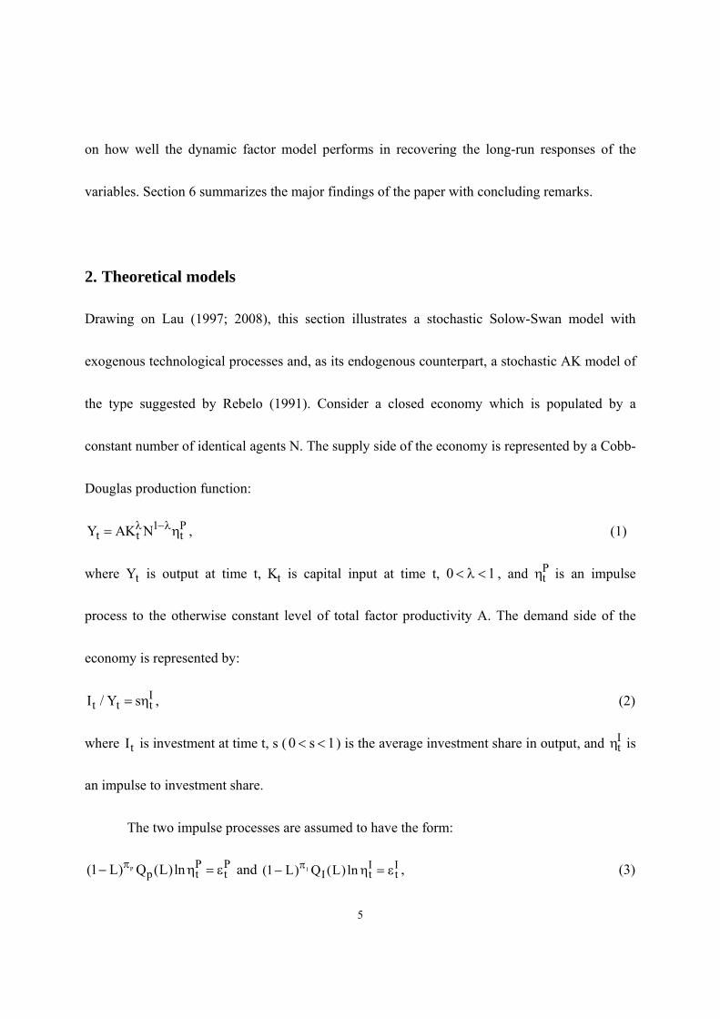
1 Pt t tY AK N , (1)
where tY is output at time t, tK is capital input at time t, 0 1 , and Pt is an impulse
process to the otherwise constant level of total factor productivity A. The demand side of the
economy is represented by:
It t tI / Y s , (2)
where tI is investment at time t, s ( 0 s 1 ) is the average investment share in output, and It is
an impulse to investment share.
The two impulse processes are assumed to have the form:
P P Pp t t(1 L) Q (L)ln and I I I
I t t(1 L) Q (L)ln , (3)

6
where L is the lag operator, j is either 0 or 1, jQ (L) is a polynomial function in L with all
roots outside the unit circle, and Pt and I
t are structural disturbances and are assumed to have a
mean of zero and an identity covariance matrix. The impulse process jtln is I(0) when j =0
and I(1) when j =1. The level of capital stock evolves over time according to
t 1 t tK (1 )K I , (4)
where ( 0 1 ) is a constant rate of depreciation.
In the Solow-Swan exogenous growth model, log per-capita output and log per-capita
investment are I(1) inherited from an I(1) process of productivity. This requires that the
productivity and investment share impulses are I(1) and I(0), respectively, and hence, P 1 and
I 0 in (3). The log-linearized equations of motion near the steady-state growth path result in
the following vector moving average (VMA) system:
t
t
(1 L)ln y
(1 L)ln i
P1 11 tP I
I1 1tP I
LQ (L) (1 L)LQ (L)(1 )L
LQ (L) (1 L)LQ (L)
, (5)
where ty and ti are per-capita output and per-capita investment, respectively.4
The AK endogenous growth model of Rebelo (1991) can be summarized using (2), (3),
(4), and
Pt t tY AK . (6)
If log per-capita output and log per-capita investment are I(1), this model implies that both
4 Appendix A provides a detailed derivation of (5).

7
productivity and investment share impulses are I(0); thus, P 0 and I 0 in (3). The log-
linearization near the steady-state growth path gives the following VMA formation:
t
t
(1 L)ln y ln(1 sA)
(1 L)ln i ln(1 sA)
1 1PP ItI1 1 tP I
1 sA1 L Q (L) L Q (L)
1 sA 1 sA
1 11 L Q (L) 1 L Q (L)
1 sA 1 sA
.5 (7)
This shows that as long as sA , the economy grows even without exogenous technological
progress.
Both Solow-Swan and AK models of growth in (5) and (7) may be rewritten compactly
as:
Pt11 12
t It 21 22 t
ln y (L) (L)constant (L) =constant
ln i (L) (L)
, (8)
where (1 L) is the first difference operator, P It t t[ , ]' is a (2x1) vector of structural
disturbances, and 20 1 2(L) L L . The long-run multiplier matrix of the Solow-
Swan model can easily be obtained from (5):
1P
i 1i 0 P
Q (1) 0(1)
Q (1) 0
. (9)
Similarly, the long-run multiplier matrix for the AK model is derived from (7) as:
5 See also Appendix A.

8
1 1P I
i1 1i 0
P I
sA sAQ (1) Q (1)
1 sA 1 sA(1)
sA sAQ (1) Q (1)
1 sA 1 sA
. (10)
In the Solow-Swan exogenous model, the first column of the long-run multiplier matrix is
non-zero and the second column is zero. A productivity shock produces permanent effects on the
levels of the variables, but a shock to investment share only causes transitory effects. In the AK
endogenous model, both columns of the long-run multiplier matrix are non-zero. The effects of
shocks to productivity and investment share are all permanent. The prediction that the transitory
investment share shock exerts permanent effects on per-capita output is a hallmark of the AK-
style models of endogenous growth. This stands in marked contrast to the Solow-Swan growth
model, in which the long-run level of per-capita output depends solely on the process of
productivity shocks. Therefore, the long-run effect of a transitory shock in investment share on
per-capita output provides a test for evaluating the empirical adequacy of Solow-Swan
exogenous and AK endogenous growth models.6
Equations (9) and (10) suggest that there is also commonality between the two models of
6 In the class of endogenous growth models, other types of shocks besides investment share may potentially have permanent effects on per-capita output. For example, Kocherlakota and Yi (1996) examined whether temporary changes in government policies, i.e., income tax rates, import tariff rates, government expenditures, and growth rate of money supply, affect the long-run level of per-capita U.S. GNP. The survey paper by Grossman and Helpman (1991) provides a summary list of potential determinants of endogenous growth. Stadler (1986) and King et al. (1988) showed that within the context of an endogenous model, any transitory shock can cause permanent effects on output, as long as it produces temporary changes in the amount of resources allocated to growth. Nonetheless, the use of AK models may well serve as a representative for determining the empirical relevancy of endogenous models because the investment variable is present in most, if not all, growth models (Lau, 2008). Jones (1995) suggests that a test based on investment data may be able to address the endogenous and exogenous growth debate for an entire class of models in the literature.

9
growth. For each structural shock, the long-run effects on the variables are identical. The reason
is that log per-capita output and log per-capita investment are cointegrated with a coefficient
vector of [1, 1 ]. This is a stochastic interpretation of balanced-growth constraints. As log per-
capita output and log per-capita investment share a common trend, the great ratio the
difference between the two becomes a stationary stochastic process along the steady-state
growth path (for details, see King et al., 1991; Neusser, 1991; Fama, 1992). One econometric
implication is that a vector error correction (VEC) model needs to be specified, which constitutes
a starting point for the estimation of parameters in the following section.
3. Empirical models
This section presents the procedure that will be in use for the empirical evaluation of Solow-
Swan exogenous and AK endogenous growth models in (9) and (10). Let t t tX [ln y , ln i ]' ,
where tln y and tln i are I(1) processes. Since the Solow-Swan and AK models posit one
cointegrating relationship with a coefficient vector of [1, 1] , the error correction term tz is
given as:
t t t tz 'X ln y ln i , (11)
where y i( , ) ' [1, 1]' is the cointegrating vector of dimension (2x1). The VEC model
may be expressed as:

10
t t 1 t(L) X constant+ z e , (12)
where 2 r1 2 r(L) I L L L , y i[ , ]' is a (2x1) vector of error correction
coefficients, and t yt ite [e , e ]' is a (2x1) vector of reduced-form disturbances with a mean of
zero and covariance matrix .
By employing the Wold decomposition and Granger’s Representation Theorem (Engle
and Granger, 1987), the VEC model in (12) can be inverted into a reduced-form VMA formation
as:
t tX constant C(L)e , (13)
where 21 2C(L) I C L C L . The long-run impacts of the reduced-form shocks on the
levels of the variable are given by C(1). Specifically, as shown in Johansen (1991):
i 'i
i 0
C(1) C L
, (14)
where and are (2x1) vectors of the orthogonal complements to and , respectively,
i.e., 0' and 0
' . is given by ' 1( (1) ) , where r
ii 1
(1) I
is a (2x2) full
rank matrix from (12). The comparison between (8) and (13) reveals the relationships between
the reduced-form and structural parameters:
t 0 te (15a)
and

11
0C(L) (L) . (15b)
Combining (13), (15a), and (15b) yields the corresponding structural VMA representation:
1t t 0 0 t tX constant C(L)e constant C(L) e (L) . (16)
The dynamic factor model we propose for empirical analysis has its origin in Stock and
Watson (1988), Johansen (1991), Kasa (1992), and Escribano and Pena (1994). Specifically, it is
assumed that
'1
0'
, (17)
and its inverse is given as:
' 1 ' 10 [ ( ) ( ) ]
. (18)
From (16) and (17), 'te and '
te are permanent and transitory shocks, respectively, and their
impacts on the variables over time are summarized in 0(L) C(L) . A key feature is that the
long-run effects of a transitory shock are not restricted to zero, but they are determined by data.
This can be verified using (14), (16), and (18), such that:
' ' 1 ' ' 10(1) C(1) [ ( ) ( ) ]
, (19)
where elements in ' ' 1( ) can be any value.
We modify (17) in such a way that the structural shocks have an identity covariance
matrix, i.e., 't tE( ) I . This can be accomplished by assuming that:

12
'11
0 1 ' 12
, (20)
where 1 T '1 1
and ' ' 12 2
. It is straightforward to check that:
't tE( ) = 1 ' T 1 T
0 t t 0 0 0E[e e ] I .
'1 te and 1 ' 1
2 te become the permanent and transitory shocks, respectively. The inverse
matrix of 10 is:
' T0 1 2[ ]
. (21)
The long-run multiplier matrix of structural shocks is calculated from (14) and (21) as:
' ' ' T0 1 2(1) C(1) [ ]
. (22)
As the implied cointegrating vector of [1, 1] ' gives [1, 1]' , (1) of dimension
(2x2) becomes:
' ' ' T1 2
' ' ' T1 2
(1)
. (23)
Equation (23) encompasses the Solow-Swan exogenous and AK endogenous growth models in
(9) and (10). This feature presents a test for distinguishing the two growth models empirically:
The determining factor is whether or not ' T2
is zero. If estimated to be zero, the evidence
is taken to support the Solow-Swan model, in which a shock to investment share exhibits only
transitory effects. If estimated to be non-zero, a shock to investment share produces permanent
effects, and, therefore, the AK model is supported empirically.

13
Lau (2008) suggests an alternative way of testing the empirical veracity of exogenous and
endogenous growth models. He assumes that 0 in (15b) is a lower triangular matrix and then
proves that if y in (12) is zero, the long-run effect of a transitory shock to investment share is
zero in support of the exogenous growth model. This proposition can be easily understood by
noting that when y 0 , ' [1 0] (see Fisher and Huh (2007) for detailed derivation). It
follows that (14) is written as C(1) [ 0] . Because 0 is lower triangular, 0C(1) (1)
of (15b) yields that 12 22(1) (1) 0 , implying no long-run effect of a shock to investment
share. If y 0 , 12 22(1) (1) 0 is refuted, and the endogenous model is chosen. While the
Lau test is easy to implement, it is only valid under the assumption that a shock to investment
share does not have a contemporaneous effect on per-capita output.
In this paper, we also consider the Beveridge and Nelson (1981) type decomposition of
permanent and transitory shocks. The model posits that:
'11
0 1 ' 12
, (24)
where 1 T '1 1
and ' ' 12 2
(Mellander et al., 1992; Englund et al., 1994;
Fisher et al., 2000). The covariance matrix of the structural shocks is
't tE( ) = 1 ' T 1 T
0 t t 0 0 0E[e e ] I . The permanent and transitory shocks are given by
'1 te and 1 ' 1
2 te , respectively. The inverse matrix of 10 is:

14
' T0 1 2[ ]
. (25)
From (16) and (25), the long-run multiplier matrix is given as:
111
0 1 11
0(1) C(1) [ 0]
0
, (26)
where the last expression is obtained with the imposition of [1, 1]' . Equation (26) is
consistent with the exogenous growth model because a shock to investment share produces only
transitory effects. Hence, it can be used to gauge how significantly the results from (23) differ
from those implied by the exogenous growth model.
4. Empirical results and discussion
4-1. Data description
Empirical analysis is undertaken with the quarterly data of output and investment in logarithms
for the G-7 countries. The measure of output is GDP. Both the output and investment series were
initially collected in nominal terms; they are divided by the GDP deflator and then divided by
population to arrive at real per-capita values. Quarterly data on population were obtained by
interpolating the annual series through the procedure INTERPOL in RATS. The sample period is
1960:1 to 2006:4, with the exception that France begins in 1970:1 due to data availability. All
data were drawn from the IMF’s International Financial Statistics (IFS).

15
4-2. Test results
To check the stationarity of the data, the order of integration of the series is examined using the
Kwiatkowski, Phillips, Schmidt, and Shin (KPSS, 1992) test; the results are reported in Table 1.
In all cases, the KPSS test rejects the null hypothesis of stationarity for the levels of the series at
the 5% significance level. When the series are first differenced, the null hypothesis of stationarity
cannot be rejected, implying that log per-capita output and log per-capita investment are
characterized as I(1) processes. This is consistent with the Solow-Swan exogenous and AK
endogenous models of growth described in Section 2.
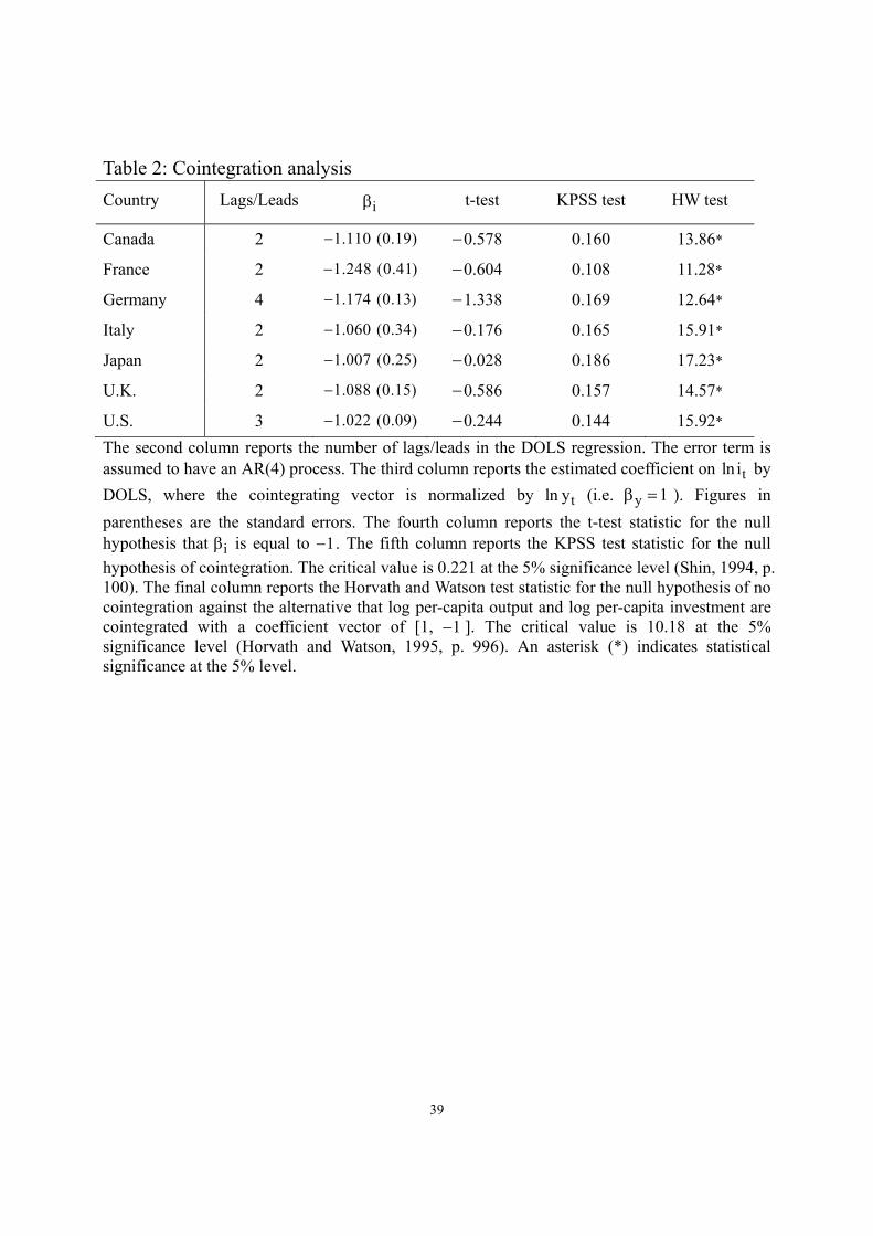
We then employ the dynamic OLS (henceforth DOLS) procedure of Stock and Watson
(1993) to test whether log per-capita output and log per-capita investment are cointegrated with a
coefficient vector of [1, 1 ].7 The DOLS procedure provides estimates of the coefficients and
their standard errors. It is also legitimate to make a statistical inference of the cointegrating
coefficients in the usual manner. Yet, in order to establish that the equation estimated by DOLS is,
in fact, a cointegrating relationship, its residuals must be shown to be stationary. The KPSS test
7 The DOLS approach has some advantages over the Johansen (1991) maximum likelihood procedure. The Johansen method, being a full information technique, is exposed to the problem that parameter estimates in one equation are affected by any misspecification in other equations. DOLS, by contrast, is a single equation approach that corrects the potential of endogeneity and small-sample bias by the inclusion of leads and lags of the first differences of the regressors, and for serially correlated errors by using GLS. Stock and Watson show, through Monte Carlo studies, that DOLS is more favorable, particularly in small samples, compared to a number of alternative estimators including that of Johansen.

16
is applied to the residuals from the DOLS regression, and the critical values tabulated by Shin
(1994) are used.8 Table 2 presents the results of the test. The number of lags/leads in the DOLS
regression was determined using the Schwarz criterion. The estimated cointegrating vectors are
normalized on log per-capita output (i.e., y 1 ).
The table shows that the KPSS test does not reject the null hypothesis of a cointegration
between log per-capita output and log per-capita investment at the 5% level of significance. The
evidence is robust across the G-7 countries. In all cases, the coefficient for tln i ( i ) is also
estimated to be close to the theoretical value of 1 . The t-test confirms this result, as it cannot
reject the null hypothesis of i 1 . Therefore, log per-capita output and log per-capita
investment are cointegrated with a coefficient vector of [1, 1 ], as implied by balanced-growth
constraints. We applied the cointegration test of Horvath and Watson (1995) as a check for
robustness. This test examines the null hypothesis of no cointegration against the alternative of
cointegration with a prespecified cointegrating vector. According to their Monte Carlo
simulations, it possesses better power properties in comparison to other competitors that do not
assume a cointegrating vector. Table 2 shows that the results remain the same. For all G-7
countries, the null hypothesis is rejected at the 5% level in favor of the cointegration relationship
between the two variables with the coefficient vector of [1, 1 ].
8 Note that the standard critical values of the KPSS test become invalid since the appropriate critical values depend on the number of regressors in the cointegrating regression.

17
Once the presence of cointegration is affirmed, VEC models are constructed in which the
error correction term is t t tz ln y ln i . The number of lags in estimation was chosen using the
Schwarz criterion. The estimated VEC models are expanded to models in the levels of the series.
They are then inverted numerically to generate estimates of the reduced-form shocks. After these
have been obtained, the structural shocks are identified, and their impacts on the series are
calculated by utilizing the procedures outlined in Section 3. At issue is the long-run response of
log per-capita output to a shock in investment share estimated from the dynamic factor
(henceforth DF) model. If it is zero, the evidence supports the exogenous growth model. If it is
significantly different from zero, the endogenous growth model is favored. Figure 1 depicts the
responses of up to 100 quarters together with 95% confidence bands generated using 500
bootstrap replications. For comparison, the corresponding figures estimated from the structural
Beveridge and Nelson (henceforth BN) model are also reported. This model assumes that the
shock to investment share produces only transitory effects on log per-capita output, consistent
with the exogenous growth model.
The results for Canada, Japan, the U.K., and the U.S. provide empirical support for the
endogenous growth model. A positive shock to investment share leads to permanent increases in
log per-capita output. The long-run effects are large and statistically different from zero at the 5%
level. In the cases of Canada and Japan, all responses are significantly different from zero across

18
the horizons. Their 95% confidence bands also exclude responses from the BN model,
confirming that the responses are empirically different from those of the exogenous growth
model associated with the BN model. The results remain virtually unchanged for the U.K. and
the U.S. The only exception is that respective responses from the DF and the BN models are
statistically indistinguishable at some initial horizons.
In contrast, results for France, Germany, and Italy support the exogenous growth model.
The long-run effects on log per-capita output of a shock to investment share are small and not
different from zero at the 5% level. In the case of Italy, the long-run responses appear to be larger
than zero, but only marginally significant. Germany shows particularly strong support for the
exogenous growth model. The responses from the DF are statistically indistinguishable from
those of the BN model across all horizons. The evidence is slightly weaker for France and Italy,
but the main finding is the same. At long horizons, the 95% confidence bands constructed from
the DF model include the responses from the BN model.
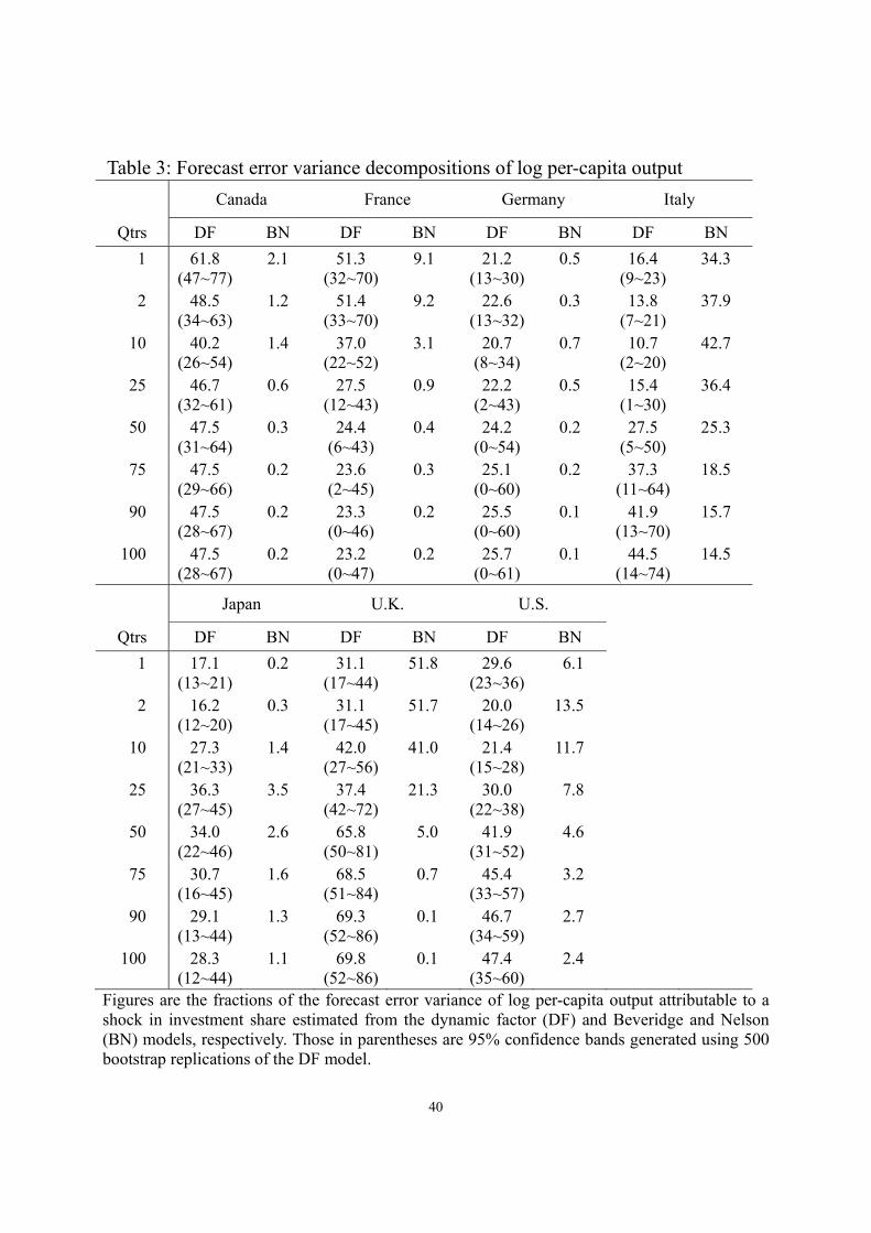
Table 3 presents the fraction of the forecast error variance of log per-capita output
attributable to a shock in investment share calculated from the DF model. Subtracting this from
100 yields the fraction that is attributable to a shock in productivity. The corresponding figures
obtained by the BN model are reported alongside. The DF model indicates that a shock to
investment share is a major determinant of long-run variation in log per-capita output for Canada,

19
the U.K. and the U.S.; it accounts for between 47% and 70% of the forecast error variance over
the horizon of 100 quarters. This shock also explains a significant portion of long-run
movements in Japan’s log per-capita output. These results are significantly different from those
of the BN model, in which the long-run contribution of the investment share shock is restricted
to zero by construction. This is to reinforce the result that Canada, Japan, the U.K., and the U.S.
support the endogenous growth model.
For France and Germany, the DF model indicates that a shock to investment share
explains a statistically insignificant fraction of the forecast error variance of log per-capita output
at long horizons. This is also consistent with our preceding results that support the exogenous
growth model. The evidence for Italy is, however, mixed. On the one hand, the contributions of a
shock to investment share to the long-run variability of log per-capita output are statistically
different from zero, which is in line with the endogenous growth model. On the other hand, their
95% confidence bands include the fractions of the forecast error variance of log per-capita that
are due to the investment share shock in the BN model. As the magnitudes between the DF and
BN models are statistically indistinguishable in the long run, the exogenous growth model is
favored. While it is difficult to make a clearcut case, the latter, assisted by the results from the
impulse response analysis, seems more revealing; hence, the exogenous growth model may be a
better description of the Italian data.

20
It is interesting to compare the results from this section with those obtained from the Lau
(2008) test in Section 3, which uses the statistical relevancy of y 0 to discriminate between
exogenous and endogenous models of growth. Table 4 reports the estimates for y and i . The
t-test shows that the coefficient y is not statistically different from zero in the G-7 countries,
except for the U.K. These six countries favor the exogenous growth model; the U.K. is the only
country receiving empirical support from the endogenous growth model. It is apparent that the
Lau test produces different results for the three countries: Canada, Japan, and the U.S. While
there are other reasons for this disparity, one may be associated with the test’s assumption that
0 is a lower triangular matrix (see Section 3). Figure 1 shows that for these countries, the
contemporaneous response of log per-capita output to a shock in investment share is statistically
different from zero. This indicates that the lower triangularity of 0 is inconsistent with the data,
raising the possibility of producing misleading implications. Indeed, the problem would not
occur if the contemporaneous responses are insignificant from zero in compliance with the
assumption; France, Germany, and Italy serve as examples where this assumption is satisfied.
Lau’s test and the DF model reach the same conclusions as shown in Table 4 and Figure 1.
4-3. Policy implications
Given that our focus is on the long-run output response to a shock in the investment share of

21
output, an immediate implication of the empirical results is that even among the G-7 countries
the appropriate long-run growth strategy should be different. That is, when it comes to
investment policy as a stimulus for long-run growth, it would be misguided to assume that there
is a “one-size-fits-all” strategy for the developed countries. Investment could be more effective
and conducive to long-run growth in some countries over others: for example, a policy focused
on encouraging investment in the US is more likely to have a positive long-run impact on output
than a similar policy in France. It is also worthwhile to note that countries whose long-run
growth are unlikely to be affected by an increase in investment share are the continental
European countries (France, Germany and Italy) while countries in the other group are English
speaking (the U.K., the U.S. and Canada) and/or tend to have high-end manufacturing bases
(Japan is a clear example in this case). Thus, our findings may suggest that an appropriate policy
design to promote long-run growth should take into account the social, legal and possibly labour
market institutions of the respective countries. This is consistent with the presumption that long-
run returns from investment would not simply depend upon the size of investment relative to
output but the complementarities associated with different policies and institutional
characteristics.9 In particular, in countries with a significant long-run output effect of investment,
policymakers need to be particularly concerned when there is a prolonged decrease in investment 9 There is a caveat, however. The policy implications concerning our results are confined to investment policy. Other policies that might have long-run impacts on growth such as education, R&D and so forth would require separate analysis and interpretation, which is beyond the scope of this paper.

22
share. The Lost Decade in Japan may be exemplary in this regard.
5. A Monte Carlo experiment
This section examines the performance of the DF model using a Monte Carlo experiment.
Consider a two-variable VEC model of t 1t 2tX [ x , x ]' :
t t 1 tX z e , (27)
where is a (2x1) vector of error correction coefficients, t t 2t 1tz 'X x x is the error
correction term, and te is a (2x1) vector of reduced-form shocks. Subject to identification, a
structural VMA representation corresponding to (27) is given as:
t tX (L) , (28)
where t 1t 2t[ , ]' is a (2x1) vector of structural shocks and is normally distributed with a
mean of zero and an identity covariance matrix. The long-run multiplier matrix (1) may be
written as:
(1)
, (29)
where and are the parameters to be determined. This follows because [ 1, 1]' and
' (1) 0 .10
10 From (15b), 0'C(1) ' (1) . Since 'C(1) 0 by the Granger’s Representation Theorem (Engle and Granger,
1987), ' (1) 0 .

23
For the present paper, the issue is the long-run effect of 2t on 1tx , denoted as in (29).
We simulate the model for nine cases where =0, 0.25 , 0.5 , 1 , and 1.5 . Details on the
data generating process are discussed further in Appendix B. The total number of simulations is
5,000 and the sample size is 200.11 In each simulation, two sets of impulse responses are
generated: One consists of true impulse responses; the other set of impulse responses is obtained
by applying the DF model. They are compared to determine how exactly the responses from the
DF model match the true ones at long horizons. For a formal test, we employ the Quasi-Lagrange
Multiplier (Q-LM) procedure of Mittnik and Zadrozny (1993) and Nason and Cogley (1994).
The Q-LM test statistic is distributed 2 (1) for the null hypothesis that there is no statistical
difference between the true and DF responses.12 Table 5 reports the percentage of replications in
which the Q-LM statistics reject the null hypothesis at the 5% level of significance.13 The
responses are at horizons of 24, 25, and 26.14
Let us first look at the testing results for the case of 0 , in which the true model
exhibits zero long-run effect of 2t on 1tx . The percentages of rejecting the null hypothesis are
11 Initially, 500 observations were generated: The first 300 observations were discarded to remove any dependence on initial values. 12 The test statistic takes the quadratic form of 1[ ]' [ ] , where is the true response, and is the DF
response. is the covariance matrix of the DF response, which is calculated as 1 Ni 1N [ (i) ][ (i) ]' ,
where (i) is the bootstrapped response of the DF procedure at replication i, and N is the total number of bootstrap
replications. N=500 is used for the application at hand. 13 The long-run responses of 2tx are not reported, since they are the same as the long-run responses of 1tx by the
cointegration restrictions. 14 All impulse response estimates completed their empirical convergence to the long-run values by 23 horizons.

24
all zero for the long-run responses of 1tx to 1t and 2t . The DF model produces the responses
that are statistically indifferent from the true responses, while it did not restrict the long-run
effect of 2t on 1tx to being zero. The evidence remains virtually the same when takes non-
zero values. The true responses are within the 95% confidence bands of the responses from the
DF model. There are a few rejections in the cases of =1 and =1.5, but the effects are minor
and do not alter the main finding. Overall, this experiment augurs well for the DF model in
capturing the long-run responses of the model.
6. Concluding remarks
This paper has examined the empirical relevance of the Solow-Swan exogenous model and AK
endogenous growth model for the G-7 countries by exploiting a key difference between the two:
whether a transitory shock to investment share exhibits permanent effects on per-capita output.
To test for this difference empirically, we develop a dynamic factor model that generates
dynamic responses of the variables to permanent and transitory shocks. The long-run effects of a
transitory shock in investment share are not restricted to being zero; they are determined from
the data. This feature presents a test for distinguishing between the exogenous and endogenous
models of growth empirically. A Monte Carlo experiment indicates that the dynamic factor
model recovers the true long-run responses of the variables.

25
Our results suggest that the endogenous growth model receives more support in Canada,
Japan, the U.K., and the U.S. A transitory shock to investment share leads to permanent increases
in log per-capita output, and the long-run effects are large and statistically different from zero. In
fact, most responses are significantly different from those of the estimated exogenous growth
model across the horizons. The investment share shock is also equally important as a shock to
productivity in accounting for the long-run variability of per-capita output. For the remaining
three countries (France, Germany, and Italy), they are more consistent with the exogenous
growth model than with the endogenous growth model.
In the literature, exogenous growth models tend to have greater empirical support from
time series studies. Different results appear to emerge, however, when a more general model for
empirical investigation is utilized. This is what the current paper shows. The endogenous growth
model responds more favorably than previous studies suggested. This result has important policy
implications because, contrary to the neoclassical presumption, raising investment share even
temporarily can have a significant long-run effect on per capita output in a number of countries.
Growth-focused policymakers in these countries may need to be particularly concerned when the
investment to output ratio is falling. Furthermore, the results from our time series approach are in
line with cross-section studies that provide empirical support for endogenous growth models.
While a more comprehensive analysis is warranted, it appears that there may be a possibility of
26
reconciling the weak support thus far obtained in the time series analysis for endogenous models
with the results from cross-section studies.
Our study provides consideration for future research. First, it is possible that government
policy choices can lead to temporary shocks to the investment share of output; however, our
approach is not designed to address the sources of such variation.15 Second, like previous studies
in the literature, we have focused on one particular testable implication of the exogenous versus
endogenous growth models. Given these limitations in the current empirics of growth models,
future studies may focus on evaluating multiple dimensions of growth models in a single
econometric framework that can utilize both time series and cross-sectional data.
15 For example, both technological change and government policy choices can influence shocks to investment share, but differentiating between these sources is beyond the scope of the current empirical study, as it requires shocks to be endogenous: a challenging econometric issue.

27
Appendix A: Derivation of the equations (5) and (7)
For succinct exposition, the derivation makes a strict reference to the equations shown in the
main section of the paper.
1. Deriving equation (5) from the neoclassical exogenous growth model
Divide through equations (1), (2) and (4) all by (1+τ)tN to transform the equations in terms of the
variables in efficiency units of labour, respectively, to get
Pt t ty Ak (1)*
/ It t ti y s (2)*
1(1 ) (1 )t t tk k i (4)*
where , and (1 ) (1 ) (1 )
t t tt t tt t t
Y K Iy k i
N N N
. Taking logs of (1)* and (2)* gives
ln ln ln ln Pt t ty A k (A-1)
ln ln ln ln It t ti y s (A-2)
To log-linearise (4)*, first divide both sides of the equation by tk
1(1 ) / (1 ) /t t t tk k i k
And then divide through by (1+τ) and re-arrange it to get
11 / (1 ) / (1 ) (1 ) ( / )t t t tk k i k
Using the technique used by Campbell (1994), take logs on both sides and using the fact that for

28
a variable Xt, Xt = exp(xt), where xt = lnXt, we get
11 1ln exp ln ln (1 )
1t t
t t
k i
k k
Given that the LHS is a function of 1 /t tk k , use a first-order Taylor approximation around the
steady state value (N.B. 1t tk k k in the steady state) to obtain
LHS 11ln t
t
k
k
Hence, the linearised equation around the steady state is
11ln ln(1 ) ln lnt
t t
t
ki k
k
Dating backward by one period and then using the lag operator, such that, for a variable Xt, LXt+1
= Xt, we get
1
1 1ln ln(1 ) lnt tL k i
(A-4)
Now take (A-1), ln ln ln ln Pt t ty A k . Divide it through by λ and then multiply
both sides by 1 1
L
to substitute out ln tk , to write as
1
1 1 1 1 1 1ln ln ln(1 ) ln
1 1 1 ln
t t
Pt
L y L A i
L
Dividing this through by 1 1
we get

29
1
1 11 ln ln ln(1 ) ln 1 ln
1 1 1 1 1P
t t tL y A i L
Taking (A-2), ln ln ln ln It t ti y s , along with the above equation, we can write them
as a system of two equations in the vector ln lnt ty i , to arrive at the following matrix system
11 ln ln
1 1 1 ( )ln
1 1 ln
11 ln
1
ln
t
t
Pt
AL L y t
i ts
L
It
(A-5)
Note that ln ln ln(1 )
tt tt
yy y t
, ln(1 ) .
To write the above (2×2) system of structural form (SF) equations in terms of a reduced
form (RF) system, solve for ln ty t and ln ti t , respectively, to get
(1 ) (1 )( )1 (ln ) ln
1 1 ( )
1 1 ln ln
1 1
t
P It t
s AL y t
L L
(A-5-1)
and
(1 ) (1 )( )1 (ln ) ln
1 1 ( )
1 1 1 ln 1 ln
1 1
t
P It t
s AL i t
L L
(A-5-2)
Now the assumption that the productivity impulse is an I(1) process while the saving rate

30
impulse is an I(0) process means πP = 1 and πI = 0, and hence the processes (3) become
P Pp t t(1 L)Q (L) ln
(A-3-1)
I II t tQ (L) ln (A-3-2)
Inverting (A-5-1) and (A-5-2) and then using the moving average form of (A-3-1) and (A-3-2) to
substitute out Ptln and I
tln , we can represent the reduced form system comprising (A-5-1) and
(A-5-2) as
1
1 1
1
(1 ) ln (1 ) (1 )( )1
(1 ) ln 1
11 ( ) (1 ) ( )
1 1
1 11 ( ) (1 ) 1
1 1
t
t
P I
P
L yL
L i
L Q L L L Q L
L Q L L
1
( )
PtIt
IL Q L
Setting τ = 0, the above system can be succinctly written as the following vector moving average
(VMA) formation [equation (5) shown in the paper].
(1 ) ln
(1 ) lnt
t
L y
L i
1 1
1
1 1
( ) (1 ) ( )(1 )
( ) (1 ) ( )
PtP IItP I
LQ L L LQ LL
LQ L L LQ L
2. Deriving equation (7) from the AK endogenous growth model
The AK model assumes the following production technology:
Pt t tY AK

31
Writing it in per capita terms and taking logs, we get
ln ln ln ln Pt t ty A k (A-6)
All other equations (2) through (4) remain the same as in the neoclassical model. The only
difference is to choose the different balanced growth path when log-linearising (4). In the AK
model, the balanced growth path with a constant population is
k y sA
Log-linearising the capital accumulation equation (4) around the balanced growth path, and then
repeating the same process leads to the analogous system
11 ln ln(1 ) ln
1 1 1ln
1 1 ln
11
1
t
t
sA sAL L y sA s
sA sA sAi
s
LsA
ln
ln
Pt
It
Solving for lnyt and lnit, and then using the moving average versions of (A-3-1) and (A-3-2)
above, we obtain the following system of equations (equation (7) shown in the paper),
1 1
1 1
11 ( ) ( )
(1 ) ln ln(1 ) 1 1
(1 ) ln ln(1 ) 1 11 ( ) 1 ( )
1 1
P I Pt t
It tP I
sAL Q L L Q L
L y sA sA sA
L i sAL Q L L Q L
sA sA
.
.

32
Appendix B: A further note on Monte Carlo experiment
For the model of (27) and (28), the following triangular VAR representation is used as a data
generating process
1t 1 t 2 t 1 1tx z z (B-1)
t 3 1t 4 t 1 2tz x z .16 (B-2)
The structural VMA representation for (B-1) and (B-2) is given as:
1t
t
x(L)
z
t . (B-3)
Premultiplying (B-3) by a (2x2) matrix and equating it with (28) yield
(L) (L) , (B-4)
where
1 0
1 1 L
.
Setting L=1 on (B-4) suggests the relationship between the two VMA representations in the long
run that:
11 12
11 12
(1) (1)(1)
(1) (1)
, (B-5)
where ij(1) is the (i, j) element of the long-run multiplier matrix (1) . Equation (B-5) shows
16 See Campbell and Shiller (1988), Mellander et al. (1992), and Lau (2008) for transforming VEC models into triangular VAR counterparts.

33
that and of (1) can be obtained by estimating (B-1) and (B-2), and calculating (B-3).
In (B-1) and (B-2), 1 , 3 , and 4 are all set to 0.3. The equations are then simulated to
generate artificial data for different values of . Nine cases are considered in the text: 1.5 ,
1 .0, 0.5 , 0.25 , 0.0, 0.25, 0.5, 1.0, and 1.5. It is easy to derive the long-run effect of 2t on
1tx as:
1 212
4 3 1 2(1)
(1 ) ( )
. (B-6)
Given 1 , 3 , and 4 , those nine cases of are provided by assuming that 2 2.209 , 1.3 ,
0.712 , 0.489 , 0.3 , 0.137 , 0.004 , 0.238, and 0.424, respectively.

34
References
Beveridge, S. and C. Nelson, 1981, A new approach to decomposition of economic time series
into permanent and transitory components with particular attention to measurement of the
business cycle, Journal of Monetary Economics 7, 151174.
Bleaney, M., Gemmell, N. and R. Neller, 2001, Testing the endogenous growth model: public
expenditure, taxation and growth over the long run, Canadian Journal of Economics 34,
36-57.
Campbell, J., 1994, Inspecting the mechanism: an analytical approach to the stochastic growth
model, Journal of Monetary Economics 33, 463-506.
Campbell, J. and R. Shiller, 1988, Interpreting cointegrated models, Journal of Economic
Dynamics and Control 12, 505522.
Cheung, Y-W, Dooley, M. and V. Sushko, 2012, Investment and Growth in Rich and Poor
Countries, National Bureau of Economic Research Working Paper No. 17788, Cambridge.
Durlauf, S., P. Johnson, and J. Temple, 2005, Growth econometrics, in P. Aghion and S. Durlauf
(eds), Handbook of Economic Growth, North-Holland, 555677.
Engle, R. and C.W.J. Granger, 1987, Cointegration and error correction: Representation,
estimation and testing, Econometrica 55, 251276.
Englund, P., A. Vredin, and A. Warne, 1994, Macroeconomic shocks in an open economy: A
common trend representation of Swedish data 1871-1990, in V. Bergström and A. Vredin
(eds), Measuring and Interpreting Business Cycles, Oxford, Clarendon Press, 125223.
Escribano, A. and D. Pena , 1994, Cointegration and common factors, Journal of Time Series
Analysis 15, 577586.
Fama, E., 1992, Transitory variation in investment and output, Journal of Monetary Economics

35
30, 467480.
Fisher, L. and H-S. Huh, 2007, Permanent-transitory decompositions under weak exogeneity,
Econometric Theory 23, 183189.
Fisher, L., H-S. Huh, and P. Summers, 2000, Structural identification of permanent shocks in
VEC models: A generalization, Journal of Macroeconomics 22, 5368.
Grossman, J. and E. Helpman, 1991, Quality ladders in the theory of growth, Review of
Economic Studies 58, 4361.
Horvath, M. and M. Watson, 1995, Testing for cointegration when some of the cointegrating
vectors are prespecified, Econometric Theory 11, 9841014.
Johansen, S., 1991, Estimation and hypothesis testing of cointegrating vectors in Gaussian vector
autoregressive models, Econometrica 59, 15511580.
Jones, C., 1995, Time series tests of endogenous growth models, Quarterly Journal of
Economics 110, 495525.
Kasa, K., 1992, Common stochastic trends in international stock markets, Journal of Monetary
Economics 29, 95124.
King, R., C. Plosser, and S. Rebelo, 1988, Production, growth and business cycles: II. New
directions, Journal of Monetary Economics 21, 309341.
King, R, C. Plosser, J. Stock, and M. Watson, 1991, Stochastic trends and economic fluctuations,
American Economic Review 81, 819840.
Kocherlakota, N. and K-M. Yi, 1996, A simple time series test of endogenous vs. exogenous
growth models: An application to the United States, Review of Economics and Statistics
78, 126134.
Kwiatkowski, D., P. Phillips, P. Schmidt, and Y. Shin, 1992, Testing the null of stationarity
against the alternative of a unit root: How sure are we that economic time series have a

36
unit root? Journal of Econometrics 54, 159178.
Lau, S-H., 1997, Using stochastic growth models to understand unit roots and breaking trends,
Journal of Economic Dynamics and Control 21, 16451667.
Lau, S-H., 2008, Using an error-correction model to test whether endogenous long-run growth
exists, Journal of Economic Dynamics and Control 32, 648676.
Lau, S-H. and C-Y. Sin, 1997, Observational equivalence and a stochastic cointegration test of
the neoclassical and Romer’s increasing returns models, Economic Modelling 14, 3960.
Levine, R. and D. Renelt, 1992, A sensitivity analysis of cross-country growth regressions,
American Economic Review 82, 942963.
Lucas, R., 1988, On the mechanisms of economic development, Journal of Monetary Economics
22, 342.
Mellander, E., A. Vredin, and A. Warne, 1992, Stochastic trends and economic fluctuations in a
small open economy, Journal of Applied Econometrics 7, 369394.
Mittnik, S. and P. Zadrozny, 1993, Asymptotic distributions of impulse responses, step responses,
and variance decompositions of estimated linear dynamic models, Econometrica 61,
857870.
Nason, J. and T. Cogley, 1994, Testing the implications of long run neutrality for monetary
business cycle models, Journal of Applied Econometrics 9, S37S70.
Neusser, K., 1991, Testing the long-run implications of the neoclassical growth model, Journal
of Monetary Economics 27, 337.
Pack, H., 1994, Endogenous growth theory: Intellectual appeal and empirical shortcomings,
Journal of Economic Perspectives 8, 5572.
Pyo, Hak K., 1995, A time series test of the endogenous growth model with human capital, in T.
Ito and A.O. Krueger (eds.) Growth Theories in Light of the East Asian Experience,

37
NBER-East Asian Studies, Vol 4, University of Chicago Press, pp. 229-245.
Rebelo, S., 1991, Long-run policy analysis and long-run growth, Journal of Political Economy
99, 500521.
Romer, P., 1986, Increasing returns and long-run growth, Journal of Political Economy 94,
10021037.
Shin, Y., 1994, A residual based test of the null of cointegration against the alternative of no
cointegration, Econometric Theory 10, 91115.
Solow, R., 1994, Perspectives on growth theory, Journal of Economic Perspectives 8, 4554.
Stadler, G., 1986, Real versus monetary business cycle theory and the statistical characteristics of
output fluctuations, Economics Letters 22, 5154.
Stock, J. and M. Watson, 1988, Testing for common trends, Journal of the American Statistical
Association 83, 10971107.
Stock, J. and M. Watson, 1993, A simple estimator of cointegrating vectors in higher order
integrated systems, Econometrica 61, 788829.

38
Table 1: Tests for unit roots
tln y tln i tln y tln i
Country no trend trend no trend trend no trend trend no trend trend
Canada 3.69* 0.65* 2.98* 0.36* 0.28 0.08 0.07 0.07
France 2.96* 0.41* 2.19* 0.15* 0.55* 0.13 0.12 0.12
Germany 3.80* 0.46* 3.40* 0.17* 0.32 0.03 0.09 0.04
Italy 3.70* 0.41* 2.87* 0.44* 0.16 0.03 0.11 0.05
Japan 3.45* 0.82* 2.89* 0.73* 0.36 0.13 0.43 0.10
U.K. 3.80* 0.23* 3.29* 0.20* 0.05 0.03 0.07 0.06
U.S. 3.79* 0.32* 3.01* 0.23* 0.10 0.03 0.04 0.03
A truncation lag is set at four. Critical values for the test are drawn from Kwiatkowski et al. (1992): They are 0.463 with no trend and 0.146 with a trend at the 5% significance level. An asterisk (*) indicates statistical significance at the 5% level.
39
Table 2: Cointegration analysis
Country Lags/Leads i t-test KPSS test HW test
Canada 2 1.110 (0.19) 0.578 0.160 13.86*
France 2 1.248 (0.41) 0.604 0.108 11.28*
Germany 4 1.174 (0.13) 1.338 0.169 12.64*
Italy 2 1.060 (0.34) 0.176 0.165 15.91*
Japan 2 1.007 (0.25) 0.028 0.186 17.23*
U.K. 2 1.088 (0.15) 0.586 0.157 14.57*
U.S. 3 1.022 (0.09) 0.244 0.144 15.92*
The second column reports the number of lags/leads in the DOLS regression. The error term is assumed to have an AR(4) process. The third column reports the estimated coefficient on tln i by
DOLS, where the cointegrating vector is normalized by tln y (i.e. y 1 ). Figures in
parentheses are the standard errors. The fourth column reports the t-test statistic for the null hypothesis that i is equal to 1 . The fifth column reports the KPSS test statistic for the null
hypothesis of cointegration. The critical value is 0.221 at the 5% significance level (Shin, 1994, p. 100). The final column reports the Horvath and Watson test statistic for the null hypothesis of no cointegration against the alternative that log per-capita output and log per-capita investment are cointegrated with a coefficient vector of [1, 1 ]. The critical value is 10.18 at the 5% significance level (Horvath and Watson, 1995, p. 996). An asterisk (*) indicates statistical significance at the 5% level.
40
Table 3: Forecast error variance decompositions of log per-capita output
Canada France Germany Italy
Qtrs DF BN DF BN DF BN DF BN
1 61.8 (47~77)
2.1 51.3 (32~70)
9.1 21.2 (13~30)
0.5 16.4 (9~23)
34.3
2 48.5 (34~63)
1.2 51.4 (33~70)
9.2 22.6 (13~32)
0.3 13.8 (7~21)
37.9
10 40.2 (26~54)
1.4 37.0 (22~52)
3.1 20.7 (8~34)
0.7 10.7 (2~20)
42.7
25 46.7 (32~61)
0.6 27.5 (12~43)
0.9 22.2 (2~43)
0.5 15.4 (1~30)
36.4
50 47.5 (31~64)
0.3 24.4 (6~43)
0.4 24.2 (0~54)
0.2 27.5 (5~50)
25.3
75 47.5 (29~66)
0.2 23.6 (2~45)
0.3 25.1 (0~60)
0.2 37.3 (11~64)
18.5
90 47.5 (28~67)
0.2 23.3 (0~46)
0.2 25.5 (0~60)
0.1 41.9 (13~70)
15.7
100 47.5 (28~67)
0.2 23.2 (0~47)
0.2 25.7 (0~61)
0.1 44.5 (14~74)
14.5
Japan U.K. U.S.
Qtrs DF BN DF BN DF BN
1 17.1 (13~21)
0.2 31.1 (17~44)
51.8 29.6 (23~36)
6.1
2 16.2 (12~20)
0.3 31.1 (17~45)
51.7 20.0 (14~26)
13.5
10 27.3 (21~33)
1.4 42.0 (27~56)
41.0 21.4 (15~28)
11.7
25 36.3 (27~45)
3.5 37.4 (42~72)
21.3 30.0 (22~38)
7.8
50 34.0 (22~46)
2.6 65.8 (50~81)
5.0 41.9 (31~52)
4.6
75 30.7 (16~45)
1.6 68.5 (51~84)
0.7 45.4 (33~57)
3.2
90 29.1 (13~44)
1.3 69.3 (52~86)
0.1 46.7 (34~59)
2.7
100 28.3 (12~44)
1.1 69.8 (52~86)
0.1 47.4 (35~60)
2.4
Figures are the fractions of the forecast error variance of log per-capita output attributable to a shock in investment share estimated from the dynamic factor (DF) and Beveridge and Nelson (BN) models, respectively. Those in parentheses are 95% confidence bands generated using 500 bootstrap replications of the DF model.

41
Table 4: Tests for error-correction coefficients
lags tln y tln i
Country y t-test i t-test
Canada 4 0.226 (0.64) 0.353 3.649 (1.71) 2.133*
France 5 0.517 (0.55) 0.940 3.197 (1.48) 2.160*
Germany 5 0.220 (0.97) 0.226 5.705 (2.77) 2.059*
Italy 8 1.256 (1.35) 0.930 5.857 (2.55) 2.296*
Japan 7 0.108 (1.05) 0.102 4.898 (1.80) 2.721*
U.K. 4 1.704 (0.85) 2.004* 5.172 (2.48) 2.085*
U.S. 6 0.954 (1.11) 0.859 7.502 (2.46) 3.049*
The second column reports the number of lags in the VEC model. The third column reports the estimate for the error correction coefficient y in the output equation. Figures in parentheses are
the standard errors. The fourth column reports the t-test statistic for the null hypothesis that y
is equal to zero. The fifth and sixth columns do the same for the investment.

42
Table 5: Monte Carlo experiments
Horizons 1 1x 2 1x 1 1x 2 1x 1 1x 2 1x 1 1x 2 1x
0
24 0 0
25 0 0
26 0 0
0.25 0.5 1 1.5
24 0 0 0 0 1 0 1 0
25 0 0 0 0 1 0 1 0
26 0 0 0 0 1 0 1 0
0.25 0.5 1 1.5
24 0 0 0 0 0 0 0 0
25 0 0 0 0 0 0 0 0
26 0 0 0 0 0 0 0 0
Figures are the percentages of replications in which the Q-LM statistics reject the null hypothesis that there is no statistical difference between the true and DF responses at the 5% significance level.

43
Figure 1: Responses of log per-capita output to a one-standard-deviation shock in investment share (percent)

44
Figure 1 (Continued)
Dynamic factor model 95% confidence bands Beveridge and Nelson model