Embed Size (px)
Citation preview
Available online at www.sciencedirect.com
Fuzzy Sets and Systems 237 (2014) 47–62
www.elsevier.com/locate/fss
An enhanced discriminability recurrent fuzzy neural network fortemporal classification problems
Gin-Der Wu ∗, Zhen-Wei Zhu
Department of Electrical Engineering, National Chi Nan University, Nantou, Taiwan, ROC
Received 30 July 2012; received in revised form 3 December 2012; accepted 15 May 2013
Available online 20 May 2013
Abstract
This paper proposes an enhanced discriminability recurrent fuzzy neural network for temporal classification problems. To con-sider classification problems, the most important consideration is the “discriminability”. To enhance the “discriminability”, thefeedback topology of the proposed fuzzy neural network is fully connected in order to handle temporal pattern behavior. Fur-thermore, the proposed fuzzy neural network considers minimum-classification-error and minimum-training-error. In minimum-classification-error, the weights are updated by maximizing the discrimination among different classes. In minimum-training-error,the parameter learning adopts the gradient descent method to reduce the cost function. Therefore, the novelty of the enhanced dis-criminability recurrent fuzzy neural network is that it not only minimizes the cost function but also maximizes the discriminability.It is constructed from structure and parameter learning. Simulations and comparisons with other recurrent fuzzy neural networksverify the performance of the enhanced discriminability recurrent fuzzy neural network under noisy conditions. Analysis resultsindicate that the proposed fuzzy neural network exhibits excellent classification performance.© 2013 Elsevier B.V. All rights reserved.
Keywords: Enhanced discriminability; Recurrent fuzzy neural network; Temporal classification; Minimum-classification-error;Minimum-training-error
1. Introduction
Feedforward fuzzy neural networks record only the static input–output correlation, making them unsuitable forthe solution of temporal classification problems. In contrast with feedforward fuzzy neural networks, recurrent fuzzyneural networks can store the past information to solve temporal problems. Since the feedback topology of recurrentfuzzy neural networks affects their ability to memorize information, several types of recurrent fuzzy neural networkshave been proposed [1–8]. The recurrent fuzzy neural networks include two categories. The first one category usesfeedback loops from the network outputs as a recurrence structure. Some studies [9,10] propose a recurrent fuzzy net-work in which the output values are fed back as input values. In another recurrent fuzzy network [11], the consequentof a rule is a reduced linear model in an autoregressive form with exogenous inputs.
* Corresponding author.E-mail address: [email protected] (G.-D. Wu).
0165-0114/$ – see front matter © 2013 Elsevier B.V. All rights reserved.http://dx.doi.org/10.1016/j.fss.2013.05.007
48 G.-D. Wu, Z.-W. Zhu / Fuzzy Sets and Systems 237 (2014) 47–62
The second category of recurrent fuzzy neural networks uses feedback loops from internal state variables as itsrecurrence structure. Recurrence can also be achieved by feeding the output of each membership function back toitself [3,6], such that each membership value is influenced by its past values. Additionally, a recurrent self-organizingneural fuzzy inference network (RSONFIN) [2] that uses a global feedback structure is proposed, in which the firingstrengths of each rule are summed up and fed back as internal network inputs. A Takagi–Sugeno (TS) type recurrentfuzzy network (TRFN) [5,8] is proposed for dynamic system processing. Another recurrent self-evolving fuzzy neuralnetwork with local feedbacks [12] is proposed for dynamic system. For processing speech patterns with temporalcharacteristics, a singleton-type recurrent neural fuzzy network (SRNFN) [13] is proposed. However, the disadvantageof the above two categories of recurrent fuzzy networks is that they consider the training data error rather than thetemporal discriminative capability.
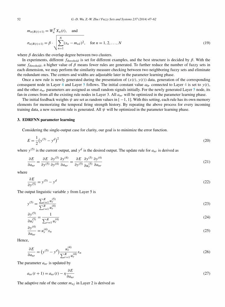
To optimize fuzzy neural networks, particle-swarm optimization (PSO) [14–16] and ant-colony optimization(ACO) [17,18] are adopted in the state-of-the-art hybrid machine learning systems. To model uncertainties, type-2fuzzy networks allow researchers to model and minimize the effects of uncertainties in rule-based systems [19–24].However, to consider the classification problems, the discriminative capability critically determines the classificationperformance. In solving classification problems, principal component analysis (PCA) has been applied in the opti-mization of classification. One study [25] proposes a self-constructing neural fuzzy inference network (SONFIN)using PCA. In a later study [26], SONFIN is applied successfully to classification problems. However, PCA lacksan analysis of the statistics among different classes, explaining why the discriminative capability of PCA is still low.Since linear discriminant analysis (LDA) is a stochastic technique that optimizes the discriminative capability amongdifferent classes, it has been extensively adopted to classify highly confusable patterns. LDA is successfully appliedin the optimization process to yield filters in order to transform a large vector into a robust vector of small dimension.A maximizing-discriminability-based self-organizing fuzzy network (MDSOFN) that can classify highly confusablepatterns is proposed [27]. Experimental and theoretical analysis results indicate that the LDA-derived fuzzy networkoutperforms the PCA-based fuzzy network and support vector machine (SVM) based fuzzy network [28–31]. How-ever, LDA suffers from the “small sample size” (SSS) problem when the signal dimension is bigger than the data size.This problem makes the within-class scatter matrix singular. Other studies [32,33] propose minimum-classification-error (MCE) methods. MCE is used to increase the temporal discriminative capability rather than to fit the distributionsto the data. The experimental results indicate that the MCE-derived filters often outperform the LDA-derived filters.Based on the concept of MCE, an enhanced discriminability recurrent fuzzy neural network (EDRFNN) for solvingclassification problems is proposed in this paper.
The rest of this paper is organized as follows. Section 2 introduces the structure learning of EDRFNN. Section 3introduces the parameter learning of EDRFNN. Section 4 demonstrates the effectiveness of the proposed EDRFNNby using two temporal classification problems. Finally, Section 5 draws conclusions.
2. EDRFNN structure learning
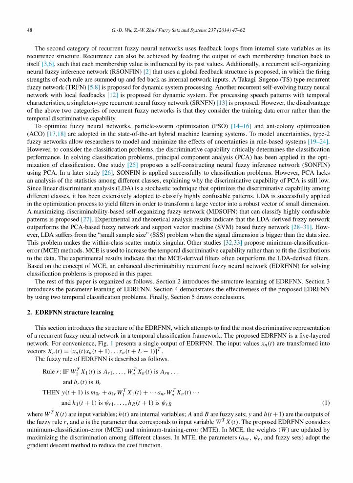
This section introduces the structure of the EDRFNN, which attempts to find the most discriminative representationof a recurrent fuzzy neural network in a temporal classification framework. The proposed EDRFNN is a five-layerednetwork. For convenience, Fig. 1 presents a single output of EDRFNN. The input values xn(t) are transformed intovectors Xn(t) = [xn(t)xn(t + 1) . . . xn(t + L − 1)]T .
The fuzzy rule of EDRFNN is described as follows.
Rule r: IF WT1 X1(t) is Ar1, . . . ,W
Tn Xn(t) is Arn . . .
and hr(t) is Br
THEN y(t + 1) is m0r + a1rWT1 X1(t) + · · ·anrW
Tn Xn(t) · · ·
and h1(t + 1) is ψr1, . . . , hR(t + 1) is ψrR (1)
where WT X(t) are input variables; h(t) are internal variables; A and B are fuzzy sets; y and h(t +1) are the outputs ofthe fuzzy rule r , and a is the parameter that corresponds to input variable WT X(t). The proposed EDRFNN considersminimum-classification-error (MCE) and minimum-training-error (MTE). In MCE, the weights (W ) are updated bymaximizing the discrimination among different classes. In MTE, the parameters (anr , ψr , and fuzzy sets) adopt thegradient descent method to reduce the cost function.
G.-D. Wu, Z.-W. Zhu / Fuzzy Sets and Systems 237 (2014) 47–62 49
Fig. 1. Structure of the enhanced discriminability recurrent fuzzy neural network (EDRFNN).
Layer 1. The nodes in this layer transform input values u(1)n (t) = xn(t) into vectors Xn(t). Then the minimum-
classification-error (MCE) weight W = [w1w2 . . .wL]T is applied to obtain the output y(1)n (t) = WT
n Xn(t).
Layer 2. Each node in this layer corresponds to one linguistic label of one input variable from Layer 1. The operationperformed in this layer is:
y(2) = exp
{− (u
(2)n − mnj )
2
σ 2nj
}(2)
where mnj and σnj are the center and the width of the Gaussian membership function of the j th term of the nth
input variable u(2)n = y
(1)n . Λ = {λm,m = 1,2, . . . , J } is a Gaussian model set where λm = N(WT μ(m),WT Σ(m)W)
represents the class m. According to the class index m, X(t) is classified and sorted as X̂(m)(n) to calculate the meanvector μ(m) and covariance matrix Σ(m):
μ(m) = 1
Nm
Nm∑n=1
X̂(m)(n) (3)
Σ(m) = 1
Nm
Nm∑n=1
(X̂(m)(n) − μ(m)
)(X̂(m)(n) − μ(m)
)T (4)
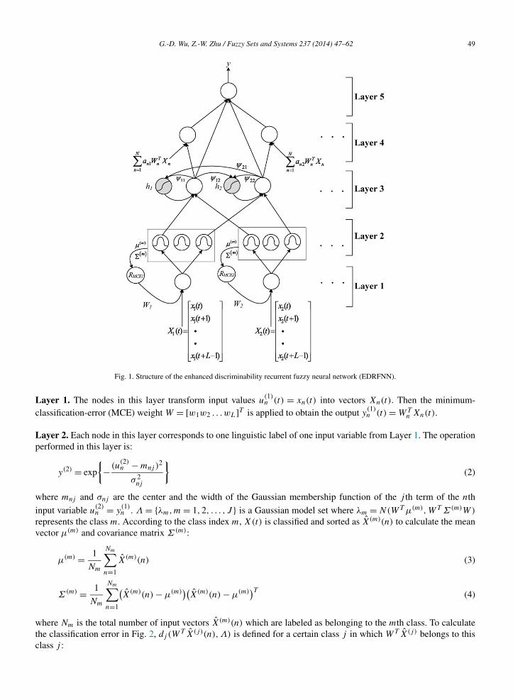
where Nm is the total number of input vectors X̂(m)(n) which are labeled as belonging to the mth class. To calculatethe classification error in Fig. 2, dj (W
T X̂(j)(n),Λ) is defined for a certain class j in which WT X̂(j) belongs to thisclass j :
50 G.-D. Wu, Z.-W. Zhu / Fuzzy Sets and Systems 237 (2014) 47–62
Fig. 2. Classification error.
dj
(WT X̂(j)(n),Λ
) = − lnP(WT X̂(j)(n)
∣∣λj
) + ln
{1
J − 1
J∑m=1m �=j
P(WT X̂(j)(n)
∣∣λm
)}(5)
where J is the total number of classes. This classification error function dj (WT X̂(j)(n),Λ) is smoothed by applying
a sigmoid function.
�(d) = 1
1 + exp(−d)(6)
Accordingly,
l(dj
(WT X̂(j)(n),Λ
)) = 1
1 + exp(−dj (WT X̂(j)(n),Λ))(7)
Then, a total loss function RMCE is defined as the smoothed classification error averaged over all the training datain all different classes:
RMCE =J∑
j=1
Nj∑n=1
l
{− lnP
(WT X̂(j)(n)
∣∣λj
) + ln
{1
J − 1
J∑m=1m �=j
P(WT X̂(j)(n)
∣∣λm
)}}(8)
where Nj is the number of patterns that belong to class j .
Layer 3. The fuzzy AND operation is used to perform the antecedent matching of the fuzzy logic rule r as follows:
fr =N∏
n=1
u(3)n (9)
The output y(3)(t) of this layer depends on not only the current rule firing strength fr but also the feedback nodey
(f )r (t)
y(3)(t) = fr · y(f )r (t) (10)
where
y(f )r (t) = 1
1 + e−hr(11)
and
G.-D. Wu, Z.-W. Zhu / Fuzzy Sets and Systems 237 (2014) 47–62 51
hr =R∑
v=1
y(3)v (t − 1) · ψvr (12)
hr is interpreted as the inference result of the feedback rule, and the feedback weight ψvr represents a fuzzy singletonvalue in the consequent part. hr uses simple weighted-sum instead of conventional average weighted-sum, hr =∑R
v=1 y(3)v (t − 1) · ψvr/
∑Rv=1 y
(3)v (t − 1). Finally, y
(f )r (t) is used to access the influence of hr , and the number of
feedback nodes is equal to the number of fuzzy rules.
Layer 4. The node is the essential node that represents a fuzzy set (Gaussian membership function) of the outputvariable. The center of each Gaussian membership function (a0r = m0r ) is delivered to the next layer for the LMOM(local mean of maximum) defuzzification operation. All WT
n Xn are assigned into this layer as follows:
y(4) = u(4)r
(N∑
n=0
anrWTn Xn
)(13)
where N is the number of input variables, and anr is the parameter that corresponds to input variable WTn Xn. In this
equation, a0rWT0 X0 with WT
0 X0 = 1 represents the center of a Gaussian membership function (a0r = m0r ).
Layer 5. Each node in this layer corresponds to one output variable. To perform the defuzzification, the node integratesall the actions recommended by Layers 3 and 4 as follows:
y(5) =∑R
r=1 u(5)r∑R
r=1 u(4)r
=∑R
r=1[u(4)r (
∑Nn=0 anrW
Tn Xn)]∑R
r=1 u(4)r
(14)
where R is the number of fuzzy rules.
There are no rules initially in EDRFNN. The criterion of clustering on the input variables is used to generate a newrule. Therefore, a cluster in the input space corresponds to a rule. The rule firing strength means the degree of theincoming pattern belongs to the corresponding cluster. An input data with high firing strength means its location iscloser to the cluster center than those with small strength. Based on this concept, the rule firing strength
y(3) =N∏
n=1
exp
{− (u
(2)n − mnj )
2
σ 2nj
}(15)
is used as the criterion to decide whether a new fuzzy rule should be generated. For the first incoming data xn(0),a new fuzzy rule is generated, with the center and width of Gaussian membership function assigned as
mn1 = WTn Xn(0) and
σn1 = σinit, for n = 1,2, . . . ,N (16)
where N is the number of input variables, and a prespecified σinit determines the initial width of the first cluster. Forsucceeding incoming data xn(t), find
I = arg max1�i�R(t)
y(3)i (17)
where R(t) is the number of existing rules at time t . If y(3)i < fthreshold(t), then a new rule is generated, where
fthreshold(t) ∈ (0,1) is a prespecified threshold that decays during the learning process as follows:
fthreshold(t) = fthreshold(t − 1)
(1 − t
Iteration_no + C
)(18)
where Iteration_no is the iteration number, and C is a constant that controls the decay speed. For a more complexlearning problem, a higher initial threshold fthreshold should be set in order to increase the rule number. Once a newrule is generated, the next step is to assign initial centers and widths of the corresponding membership functions as
52 G.-D. Wu, Z.-W. Zhu / Fuzzy Sets and Systems 237 (2014) 47–62
mn(R(t)+1) = WTn Xn(t), and
σn(R(t)+1) = β ·√√√√ N∑
n=1
(xn − mnI )2, for n = 1,2, . . . ,N (19)
where β decides the overlap degree between two clusters.In experiments, different fthreshold is set for different examples, and the best structure is decided by β . With the
same fthreshold , a higher value of β means fewer rules are generated. To further reduce the number of fuzzy sets ineach dimension, we may perform the similarity measure checking between two neighboring fuzzy sets and eliminatethe redundant ones. The centers and widths are adjustable later in the parameter learning phase.
Once a new rule is newly generated during the presentation of (x(t), y(t)) data, generation of the correspondingconsequent node in Layer 4 and Layer 5 follows. The initial constant value a0r connected to Layer 4 is set to y(t),and the other anr parameters are assigned as small random signals initially. For the newly generated Layer 5 node, itsfan-in comes from all the existing rule nodes in Layer 3. All anr will be optimized in the parameter learning phase.
The initial feedback weights ψ are set as random values in [ −1,1]. With this setting, each rule has its own memoryelements for memorizing the temporal firing strength history. By repeating the above process for every incomingtraining data, a new recurrent rule is generated. All ψ will be optimized in the parameter learning phase.
3. EDRFNN parameter learning
Considering the single-output case for clarity, our goal is to minimize the error function.
E = 1
2
(y(5) − yd
)2 (20)
where y(5) is the current output, and yd is the desired output. The update rule for anr is derived as
∂E
∂anr
= ∂E
∂y(5)
∂y(5)
∂y(4)
∂y(4)
∂anr
= ∂E
∂y(5)
∂y(5)
∂u(5)r
∂y(4)
∂anr
(21)
where
∂E
∂y(5)= y(5) − yd (22)
The output linguistic variable y from Layer 5 is
y(5) =∑R
r=1 u(5)r∑R
r=1 u(4)r
(23)
∂y(5)
∂u(5)r
= 1∑Rr=1 u
(4)r
(24)
∂y(4)
∂anr
= u(4)r xn (25)
Hence,
∂E
∂anr
= (y(5) − yd
) u(4)r∑R
r=1 u(4)r
xn (26)
The parameter anr is updated by
anr(t + 1) = anr(t) − η∂E
∂anr
(27)
The adaptive rule of the center mnj in Layer 2 is derived as
G.-D. Wu, Z.-W. Zhu / Fuzzy Sets and Systems 237 (2014) 47–62 53
∂E
∂mnj
= ∂E
∂y(5)
∂y(5)
∂y(3)
∂y(3)
∂y(2)
∂y(2)
∂mnj
= ∂E
∂y(5)
∂y(5)
∂u(4)r
∂y(3)
∂u(3)i
∂y(2)
∂mnj
(28)
where
∂E
∂y(5)= y(5) − yd (29)
∂y(5)
∂u(4)r
= ∂
∂u(4)r
{∑Rr=1[u(4)
r (∑N
n=0 anrxn)]∑Rr=1 u
(4)r
}=
∑Nn=0 anrxn − y(5)∑R
r=1 u(4)r
(30)
∂y(3)
∂u(3)n
= ∂
∂u(3)n
{ ∏Nk=1 u
(3)k
1 + exp[−∑Rv=1 y
(3)v (t − 1) · ψvr ]
}=
∏Nk=1, k �=n u
(3)k
1 + exp[−∑Rv=1 y
(3)v (t − 1) · ψvr ]
(31)
∂y(2)
∂mnj
= efn · 2(u(2)n − mnj )
σ 2nj
and fn = − (u(2)n − mnj )
2
σ 2nj
(32)
Hence,
∂E
∂mnj
= (y(5) − yd
) ·∑N
n=0 anrxn − y(5)∑Rr=1 u
(4)r
·∏N
k=1 u(3)k
1 + exp[−∑Rv=1 y
(3)v (t − 1) · ψvr ]
· 2(u(2)n − mnj )
σ 2nj
(33)
So the update rule of mnj in Layer 2 is
mnj (t + 1) = mnj (t) − η∂E
∂mnj
(34)
Similarly, the update rule of σnj in Layer 2 is
∂E
∂σnj
= ∂E
∂y(5)
∂y(5)
∂y(3)
∂y(3)
∂y(2)
∂y(2)
∂σnj
= (y(5) − yd
) ·∑N
n=0 anrxn − y(5)∑Rr=1 u
(4)r
·∏N
k=1 u(3)k
1 + exp[−∑Rv=1 y
(3)v (t − 1) · ψvr ]
· 2(u(2)n − mnj )
2
σ 3nj
(35)
So the update rule of σnj in Layer 2 is
σnj (t + 1) = σnj (t) − η∂E
∂σnj
(36)
The update rule for the feedback weight ψr is derived as
∂E
∂ψvr
= ∂E
∂y(5)
∂y(5)
∂y(3)
∂y(3)
∂ψvr
= ∂E
∂y(5)
∂y(5)
∂u(4)r
∂y(3)
∂ψvr
(37)
where
∂y(3)
∂ψvr
= ∂
∂ψvr
{ ∏Nn=1 u
(3)n
1 + exp[−∑Rv=1 y
(3)v (t − 1) · ψvr ]
}
=(
N∏n=1
u(3)n
)· y(f )
r (t) · [1 − y(f )r (t)
] · y(3)v (t − 1) (38)
Hence,
∂E
∂ψvr
= (y(5) − yd
) ·∑N
n=0 anrxn − y(5)∑Ru
(4)·(
N∏u(3)
n
)· y(f )
r (t) · [1 − y(f )r (t)
] · y(3)v (t − 1) (39)
r=1 r n=1
54 G.-D. Wu, Z.-W. Zhu / Fuzzy Sets and Systems 237 (2014) 47–62
So the update rule of ψjr is
ψvr(t + 1) = ψvr(t) − η∂E
∂ψvr
(40)
To maximize the discriminative capability, the Gaussian model of MCE is shown as follows:
P(WT X̂(j)(n)
∣∣λm
) = N(WT X̂(j)(n);WT μ(m),WT Σ(m)W
)= 1√
2πWT Σ(m)W× e
− 12 × (WT X̂(j)(n)−WT μ(m))2
WT Σ(m)W (41)
The total loss function RMCE is defined as
RMCE =J∑
j=1
Nj∑n=1
l
{− lnP
(WT X̂(j)(n)
∣∣λj
) + ln
{1
J − 1
J∑m=1m �=j
P(WT X̂(j)(n)
∣∣λm
)}}
=J∑
j=1
Nj∑n=1
l
{− lnN
(WT X̂(j)(n);WT μ(j),WT Σ(j)W
)
+ ln
[1
J − 1
J∑m=1m �=j
N(WT X̂(j)(n);WT μ(m),WT Σ(m)W
)]}(42)
where lnN(WT X̂(j)(n);WT μ(j),WT Σ(j)W) is related to the class-conditioned likelihood.
ln
[1
J − 1
J∑m=1,m �=j
N(WT X̂(j)(n);WT μ(m),WT Σ(m)W
)]
is a function that defines how the class-conditioned likelihoods for the competing models λm, m = 1,2, . . . , J , m �= j ,are counted in the classification error function. Next, the classification error function is smoothed by applying asigmoid function �(d) in (6). To maximize the discriminative capability, RMCE is differentiated with respect to W asfollows:
∂RMCE
∂W=
J∑j=1
N∑n=1
∂l
∂dj
∂dj (WT X̂(j)(n),Λ)
∂W(43)
where
∂l
∂dj
= αl(dj )(1 − l(dj )
)(44)
∂
∂Wdj
(WT X̂(j)(n),Λ
)= − ∂
∂WlnP
(WT X̂(j)(n)
∣∣λj
) + ∂
∂Wln
(1
J − 1
)+ ∂
∂Wln
(J∑
m=1m �=j
P(WT X̂(j)(n)
∣∣λm
))
= − ∂
∂WlnP
(WT X̂(j)(n)
∣∣λj
) +∑J
m=1,m �=j P ′(WT X̂(j)(n)|λm)∑Jm=1,m �=j P (WT X̂(j)(n)|λm)
= − ∂
∂WlnP
(WT X̂(j)(n)
∣∣λj
) +∑J
m=1,m �=j [P(WT X̂(j)(n)|λm)P ′(WT X̂(j)(n)|λm)
P (WT X̂(j)(n)|λm)]∑J
m=1,m �=j P (WT X(j)(n)|λm)(45)
and
P ′(WT X̂(j)(n)|λm)
T ˆ (j)= ∂
∂WlnP
(WT X̂(j)(n)
∣∣λm
)(46)
P(W X (n)|λm)
G.-D. Wu, Z.-W. Zhu / Fuzzy Sets and Systems 237 (2014) 47–62 55
Then
∂
∂Wdj
(WT X̂(j)(n),Λ
) =
{ ∑Jm=1,m �=j {P(WT X̂(j)(n)|λm)[ ∂
∂WlnP(WT X̂(j)(n)|λm)]}
− {∑Jm=1,m �=j P (WT X̂(j)(n)|λm)}[ ∂
∂WlnP(WT X̂(j)(n)|λj )]
}∑J
m=1,m �=j P (WT X̂(j)(n)|λm)
=∑J
m=1,m �=j
{P(WT X̂(j)(n)|λm)[ ∂
∂WlnP(WT X̂(j)(n)|λm)
− ∂∂W
lnP(WT X̂(j)(n)|λj )]}
∑Jm=1,m �=j P (WT X̂(j)(n)|λm)
(47)
where
∂
∂WlnP
(WT X̂(j)(n)
∣∣λm
)= ∂
∂Wln
{1√
2πWT Σ(m)W× e
− 12 × (WT X̂(j)(n)−WT μ(m))2
WT Σ(m)W
}
= ∂
∂W
(−1
2ln 2π
)+ ∂
∂W
(−1
2ln
(WT Σ(m)W
)) − 1
2
∂
∂W
{ [WT (X̂(j)(n) − μ(m))]2
WT Σ(m)W
}
= −1
2
2Σ(m)W
WT Σ(m)W− 1
2
∂
∂W
[WT (X̂(j)(n) − μ(m))(X̂(j)(n) − μ(m))T W
WT Σ(m)W
]
= − Σ(m)W
WT Σ(m)W− 1
2
1
(WT Σ(m)W)2
{[WT
(X̂(j)(n) − μ(m)
)(X̂(j)(n) − μ(m)
)TW
]′(WT Σ(m)W
)− [
WT(X̂(j)(n) − μ(m)
)(X̂(j)(n) − μ(m)
)TW
](WT Σ(m)W
)′}= − Σ(m)W
WT Σ(m)W− 1
2
1
(WT Σ(m)W)2
{[2(X̂(j)(n) − μ(m)
)(X̂(j)(n) − μ(m)
)TW
](WT Σ(m)W
)− [
WT(X̂(j)(n) − μ(m)
)(X̂(j)(n) − μ(m)
)TW
](2Σ(m)W
)}= − Σ(m)W
WT Σ(m)W− 1
(WT Σ(m)W)2
{[(X̂(j)(n) − μ(m)
)(X̂(j)(n) − μ(m)
)TW
](WT Σ(m)W
)− [
WT(X̂(j)(n) − μ(m)
)(X̂(j)(n) − μ(m)
)TW
](Σ(m)W
)}(48)
To minimize RMCE , W is updated as follows:
W(t + 1) = W(t) − ηt
∂RMCE
∂W
∣∣∣∣W=W(t)
(49)
and
∂RMCE
∂W=
J∑j=1
N∑n=1
∂l
∂dj
∂dj (WT X̂(j)(n),Λ)
∂W(50)
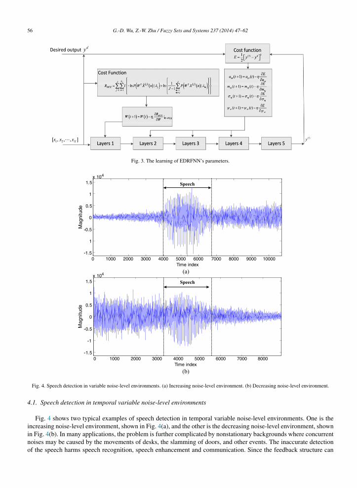
The flowchart of EDRFNN parameter learning is shown in Fig. 3.
4. Experiments
Effectiveness of the proposed EDRFNN is evaluated by two temporal classification problems. The first is speechdetection in temporal variable noise-level environments, and the second is speech recognition under noisy environ-ments. Other recurrent fuzzy neural networks, including singleton-type recurrent neural fuzzy network (SRNFN) [13],TS-type recurrent fuzzy network (TRFN) [5], and TS-type maximizing-discriminability-based recurrent fuzzy net-work MDRFN [34] are tested. For further comparison, MDRFN without MCE is proposed as simple recurrent fuzzynetwork (SRFN).
56 G.-D. Wu, Z.-W. Zhu / Fuzzy Sets and Systems 237 (2014) 47–62
Fig. 3. The learning of EDRFNN’s parameters.
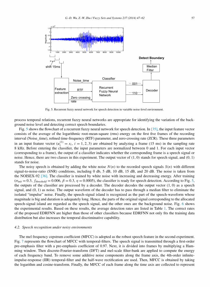
Fig. 4. Speech detection in variable noise-level environments. (a) Increasing noise-level environment. (b) Decreasing noise-level environment.
4.1. Speech detection in temporal variable noise-level environments
Fig. 4 shows two typical examples of speech detection in temporal variable noise-level environments. One is theincreasing noise-level environment, shown in Fig. 4(a), and the other is the decreasing noise-level environment, shownin Fig. 4(b). In many applications, the problem is further complicated by nonstationary backgrounds where concurrentnoises may be caused by the movements of desks, the slamming of doors, and other events. The inaccurate detectionof the speech harms speech recognition, speech enhancement and communication. Since the feedback structure can
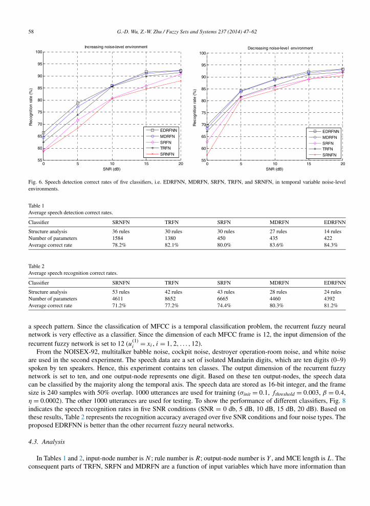
G.-D. Wu, Z.-W. Zhu / Fuzzy Sets and Systems 237 (2014) 47–62 57
Fig. 5. Recurrent fuzzy neural network for speech detection in variable noise-level environment.
process temporal relations, recurrent fuzzy neural networks are appropriate for identifying the variation of the back-ground noise level and detecting correct speech boundaries.
Fig. 5 shows the flowchart of a recurrent fuzzy neural network for speech detection. In [35], the input feature vectorconsists of the average of the logarithmic root-mean-square (rms) energy on the first five frames of the recordinginterval (Noise_time), refined time-frequency (RTF) parameter, and zero-crossing rate (ZCR). These three parametersin an input feature vector (u(1)
i = xi , i = 1,2,3) are obtained by analyzing a frame (15 ms) in the sampling rate8 kHz. Before entering the classifier, the input parameters are normalized between 0 and 1. For each input vector(corresponding to a frame), the output of a classifier indicates whether the corresponding frame is a speech signal ornoise. Hence, there are two classes in this experiment. The output vector of (1,0) stands for speech signal, and (0,1)
stands for noise.The noisy speech is obtained by adding the white noise N(n) to the recorded speech signals S(n) with different
signal-to-noise-ratio (SNR) conditions, including 0 db, 5 dB, 10 dB, 15 dB, and 20 dB. The noise is taken fromthe NOISEX-92 [36]. The classifier is trained by white noise with increasing and decreasing energy. After training(σinit = 0.3, fthreshold = 0.006, β = 0.3, η = 0.0005), the classifier is ready for speech detection. According to Fig. 5,the outputs of the classifier are processed by a decoder. The decoder decodes the output vector (1,0) as a speechsignal, and (0,1) as noise. The output waveform of the decoder has to pass through a median filter to eliminate theisolated “impulse” noise. Finally, the speech-signal island is recognized as the part of the speech-waveform whosemagnitude is big and duration is adequately long. Hence, the parts of the original signal corresponding to the allocatedspeech-signal island are regarded as the speech signal, and the other ones are the background noise. Fig. 6 showsthe experimental results. Based on these results, the average detection rates are listed in Table 1. The correct ratesof the proposed EDRFNN are higher than those of other classifiers because EDRFNN not only fits the training datadistribution but also increases the temporal discriminative capability.
4.2. Speech recognition under noisy environments
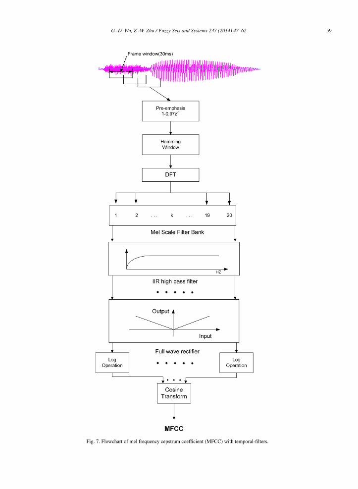
The mel frequency cepstrum coefficient (MFCC) is adopted as the robust speech feature in the second experiment.Fig. 7 represents the flowchart of MFCC with temporal-filters. The speech signal is transmitted through a first-orderpre-emphasis filter with a pre-emphasis coefficient of 0.97. Next, it is divided into frames by multiplying a Ham-ming window. Then discrete-Fourier-transform (DFT) and mel-scale filter-bank are applied to compute the energyof each frequency band. To remove some additive noise components along the frame axis, the 4th-order infinite-impulse-response (IIR) temporal-filter and the half-wave rectification are used. Then, MFCC is obtained by takingthe logarithm and cosine-transform. Finally, the MFCC of each frame along the time axis are collected to represent
58 G.-D. Wu, Z.-W. Zhu / Fuzzy Sets and Systems 237 (2014) 47–62
Fig. 6. Speech detection correct rates of five classifiers, i.e. EDRFNN, MDRFN, SRFN, TRFN, and SRNFN, in temporal variable noise-levelenvironments.
Table 1Average speech detection correct rates.
Classifier SRNFN TRFN SRFN MDRFN EDRFNN
Structure analysis 36 rules 30 rules 30 rules 27 rules 14 rulesNumber of parameters 1584 1380 450 435 422Average correct rate 78.2% 82.1% 80.0% 83.6% 84.3%
Table 2Average speech recognition correct rates.
Classifier SRNFN TRFN SRFN MDRFN EDRFNN
Structure analysis 53 rules 42 rules 43 rules 28 rules 24 rulesNumber of parameters 4611 8652 6665 4460 4392Average correct rate 71.2% 77.2% 74.4% 80.3% 81.2%
a speech pattern. Since the classification of MFCC is a temporal classification problem, the recurrent fuzzy neuralnetwork is very effective as a classifier. Since the dimension of each MFCC frame is 12, the input dimension of therecurrent fuzzy network is set to 12 (u(1)
i = xi , i = 1,2, . . . ,12).From the NOISEX-92, multitalker babble noise, cockpit noise, destroyer operation-room noise, and white noise
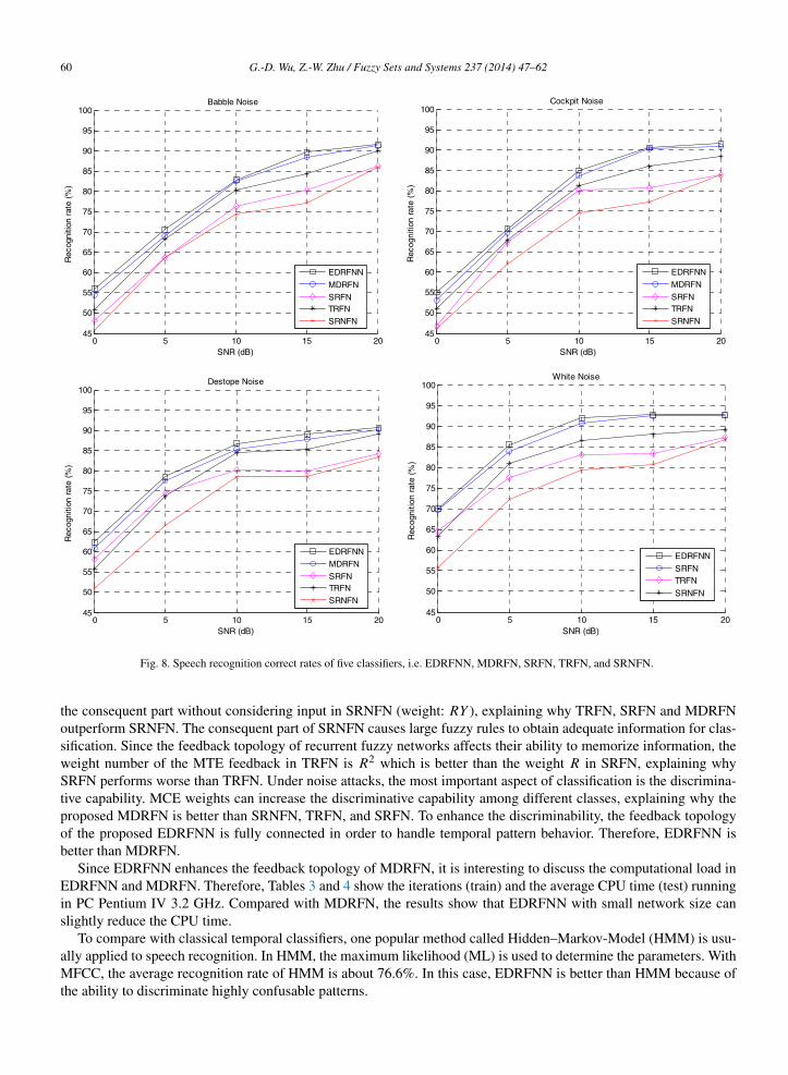
are used in the second experiment. The speech data are a set of isolated Mandarin digits, which are ten digits (0–9)spoken by ten speakers. Hence, this experiment contains ten classes. The output dimension of the recurrent fuzzynetwork is set to ten, and one output-node represents one digit. Based on these ten output-nodes, the speech datacan be classified by the majority along the temporal axis. The speech data are stored as 16-bit integer, and the framesize is 240 samples with 50% overlap. 1000 utterances are used for training (σinit = 0.1, fthreshold = 0.003, β = 0.4,η = 0.0002). The other 1000 utterances are used for testing. To show the performance of different classifiers, Fig. 8indicates the speech recognition rates in five SNR conditions (SNR = 0 db, 5 dB, 10 dB, 15 dB, 20 dB). Based onthese results, Table 2 represents the recognition accuracy averaged over five SNR conditions and four noise types. Theproposed EDRFNN is better than the other recurrent fuzzy neural networks.
4.3. Analysis
In Tables 1 and 2, input-node number is N ; rule number is R; output-node number is Y , and MCE length is L. Theconsequent parts of TRFN, SRFN and MDRFN are a function of input variables which have more information than
G.-D. Wu, Z.-W. Zhu / Fuzzy Sets and Systems 237 (2014) 47–62 59
Fig. 7. Flowchart of mel frequency cepstrum coefficient (MFCC) with temporal-filters.
60 G.-D. Wu, Z.-W. Zhu / Fuzzy Sets and Systems 237 (2014) 47–62
Fig. 8. Speech recognition correct rates of five classifiers, i.e. EDRFNN, MDRFN, SRFN, TRFN, and SRNFN.
the consequent part without considering input in SRNFN (weight: RY ), explaining why TRFN, SRFN and MDRFNoutperform SRNFN. The consequent part of SRNFN causes large fuzzy rules to obtain adequate information for clas-sification. Since the feedback topology of recurrent fuzzy networks affects their ability to memorize information, theweight number of the MTE feedback in TRFN is R2 which is better than the weight R in SRFN, explaining whySRFN performs worse than TRFN. Under noise attacks, the most important aspect of classification is the discrimina-tive capability. MCE weights can increase the discriminative capability among different classes, explaining why theproposed MDRFN is better than SRNFN, TRFN, and SRFN. To enhance the discriminability, the feedback topologyof the proposed EDRFNN is fully connected in order to handle temporal pattern behavior. Therefore, EDRFNN isbetter than MDRFN.
Since EDRFNN enhances the feedback topology of MDRFN, it is interesting to discuss the computational load inEDRFNN and MDRFN. Therefore, Tables 3 and 4 show the iterations (train) and the average CPU time (test) runningin PC Pentium IV 3.2 GHz. Compared with MDRFN, the results show that EDRFNN with small network size canslightly reduce the CPU time.
To compare with classical temporal classifiers, one popular method called Hidden–Markov-Model (HMM) is usu-ally applied to speech recognition. In HMM, the maximum likelihood (ML) is used to determine the parameters. WithMFCC, the average recognition rate of HMM is about 76.6%. In this case, EDRFNN is better than HMM because ofthe ability to discriminate highly confusable patterns.
G.-D. Wu, Z.-W. Zhu / Fuzzy Sets and Systems 237 (2014) 47–62 61
Table 3Computational load of EDRFNN and MDRFN in Experiment A.
Classifier MDRFN EDRFNN
Train: iterations 2000 2000Test: CPU time (s) 0.6 0.58
Table 4Computational load of EDRFNN and MDRFN in Experiment B.
Classifier MDRFN EDRFNN
Train: iterations 800 800Test: CPU time (s) 1.4 1.37
5. Conclusions
This paper proposes an enhanced discriminability recurrent fuzzy neural network (EDRFNN) for temporal classi-fication problems. Since the feedback topology of recurrent fuzzy neural networks affects their ability to memorizeinformation, the feedback topology of the proposed EDRFNN is fully connected in order to handle temporal patternbehavior. Besides, the proposed EDRFNN considers minimum-classification-error (MCE) and minimum-training-error (MTE). In MCE, the weights are updated by maximizing the discrimination among different classes. In MTE, theparameter learning adopts the gradient descent method to reduce the cost function. Therefore, the proposed EDRFNNis characterized by its ability to minimize the cost function and maximize the discriminative capability. Finally, theproposed EDRFNN is evaluated by two temporal classification problems. Experimental results indicate that EDRFNNcan classify highly confusable temporal patterns with a small network structure.
References
[1] M.A.G. Olvera, Y. Tang, A new recurrent neurofuzzy network for identification of dynamic systems, Fuzzy Sets Syst. 158 (10) (2007) 1023–1035.
[2] C.F. Juang, C.T. Lin, A recurrent self-organizing neural fuzzy inference network, IEEE Trans. Neural Netw. 10 (4) (1999) 828–845.[3] C.H. Lee, C.C. Teng, Identification and control of dynamic systems using recurrent fuzzy neural networks, IEEE Trans. Fuzzy Syst. 8 (4)
(2000) 349–366.[4] P.A. Mastorocostas, J.B. Theocharis, A recurrent fuzzy-neural model for dynamic system identification, IEEE Trans. Syst. Man Cybern.,
Part B, Cybern. 32 (2) (2002) 176–190.[5] C.F. Juang, A TSK-type recurrent fuzzy network for dynamic systems processing by neural network and genetic algorithm, IEEE Trans. Fuzzy
Syst. 10 (2) (2002) 155–170.[6] C.J. Lin, C.C. Chin, Prediction and identification using wavelet-based recurrent fuzzy neural networks, IEEE Trans. Syst. Man Cybern., Part B,
Cybern. 34 (5) (2004) 2144–2154.[7] Y. Gao, M.J. Er, NARMAX time series model prediction: Feedforward and recurrent fuzzy neural network approaches, Fuzzy Sets Syst. 150
(2005) 331–350.[8] C.F. Juang, J.S. Chen, Water bath temperature control by a recurrent fuzzy controller and its FPGA implementation, IEEE Trans. Ind. Electron.
53 (3) (2006) 941–949.[9] G. Mouzouris, J.M. Mendel, Dynamic non-singleton fuzzy logic systems for nonlinear modeling, IEEE Trans. Fuzzy Syst. 5 (2) (1997)
199–208.[10] Y.C. Wang, C.J. Chien, C.C. Teng, Direct adaptive iterative learning control of nonlinear systems using an output-recurrent fuzzy neural
network, IEEE Trans. Syst. Man Cybern., Part B, Cybern. 34 (3) (2004) 1348–1359.[11] J. Zhang, A.J. Morris, Recurrent neuro-fuzzy networks for nonlinear process modeling, IEEE Trans. Neural Netw. 10 (2) (1999) 313–326.[12] C.F. Juang, Y.Y. Lin, C.C. Tu, A recurrent self-evolving fuzzy neural network with local feedbacks and its application to dynamic system
processing, Fuzzy Sets Syst. 161 (19) (2010) 2552–2568.[13] C.F. Juang, C.T. Chiou, C.L. Lai, Hierarchical singleton-type recurrent neural fuzzy networks for noisy speech recognition, IEEE Trans.
Neural Netw. 18 (3) (2007) 833–843.[14] M.A. Shoorehdeli, M. Teshnehlab, A.K. Sedigh, Training ANFIS as an identifier with intelligent hybrid stable learning algorithm based on
particle swarm optimization and extended Kalman filter, Fuzzy Sets Syst. 160 (7) (2009) 922–948.[15] R.K. Brouwer, A. Groenwold, Modified fuzzy c-means for ordinal valued attributes with particle swarm for optimization, Fuzzy Sets Syst.
161 (13) (2010) 1774–1789.[16] S.K. Oh, W.D. Kim, W. Pedrycz, B.J. Park, Polynomial-based radial basis function neural networks (P-RBF NNs) realized with the aid of
particle swarm optimization, Fuzzy Sets Syst. 163 (1) (2011) 54–77.
62 G.-D. Wu, Z.-W. Zhu / Fuzzy Sets and Systems 237 (2014) 47–62
[17] R. Jensen, Q. Shen, Fuzzy-rough data reduction with ant colony optimization, Fuzzy Sets Syst. 149 (1) (2005) 5–20.[18] C.F. Juang, C. Lo, Zero-order TSK-type fuzzy system learning using a two-phase swarm intelligence algorithm, Fuzzy Sets Syst. 159 (21)
(2008) 2910–2926.[19] C.F. Juang, R.B. Huang, Y.Y. Lin, A recurrent self-evolving interval type-2 fuzzy neural network for dynamic system processing, IEEE Trans.
Fuzzy Syst. 17 (5) (2009) 1092–1105.[20] F.J. Lin, P.H. Chou, Adaptive control of two-axis motion control system using interval type-2 fuzzy neural network, IEEE Trans. Ind. Electron.
56 (1) (2009) 178–193.[21] C.F. Juang, C.H. Hsu, Reinforcement interval type-2 fuzzy controller design by online rule generation and Q-value-aided ant colony optimiza-
tion, IEEE Trans. Syst. Man Cybern., Part B, Cybern. 39 (6) (2009) 1528–1542.[22] C.F. Juang, R.B. Huang, W.Y. Cheng, An interval type-2 fuzzy-neural network with support-vector regression for noisy regression problems,
IEEE Trans. Fuzzy Syst. 18 (4) (2010) 686–699.[23] X. Du, H. Ying, Derivation and analysis of the analytical structures of the interval type-2 fuzzy-PI and PD controllers, IEEE Trans. Fuzzy
Syst. 18 (4) (2010) 802–814.[24] M. Biglarbegian, W.W. Melek, J.M. Mendel, On the stability of interval type-2 TSK fuzzy logic control systems, IEEE Trans. Syst. Man
Cybern., Part B, Cybern. 40 (3) (2010) 798–818.[25] C.F. Juang, C.T. Lin, An on-line self-constructing neural fuzzy inference network and its applications, IEEE Trans. Fuzzy Syst. 6 (1) (1998)
12–32.[26] G.D. Wu, C.T. Lin, Word boundary detection with mel-scale frequency bank in noisy environment, IEEE Trans. Speech Audio Process. 8 (5)
(2000) 541–554.[27] G.D. Wu, P.H. Huang, A maximizing-discriminability-based self-organizing fuzzy network for classification problems, IEEE Trans. Fuzzy
Syst. 18 (2) (2010) 362–373.[28] J.H. Chiang, P.Y. Hao, Support vector learning mechanism for fuzzy rule-based modeling: A new approach, IEEE Trans. Fuzzy Syst. 12 (1)
(2004) 1–12.[29] Y. Chen, J.Z. Wang, Support vector learning for fuzzy rule-based classification systems, IEEE Trans. Fuzzy Syst. 11 (6) (2003) 716–728.[30] C.T. Lin, C.M. Yeh, S.F. Liang, J.F. Chung, N. Kumar, Support-vector-based fuzzy neural network for pattern classification, IEEE Trans.
Fuzzy Syst. 14 (1) (2006) 31–41.[31] C.F. Juang, S.H. Chiu, S.W. Chang, A self-organizing TS-type fuzzy network with support vector learning and its application to classification
problems, IEEE Trans. Fuzzy Syst. 15 (5) (2007) 997–1008.[32] A. Biem, Minimum classification error training for online handwriting recognition, IEEE Trans. Pattern Anal. Mach. Intell. 28 (7) (2006)
1041–1051.[33] J.W. Hung, L.S. Lee, Optimization of temporal filters for constructing robust features in speech recognition, IEEE Trans. Audio Speech Lang.
Process. 14 (3) (2006) 808–832.[34] G.D. Wu, Z.W. Zhu, P.H. Huang, A TS-type maximizing-discriminability-based recurrent fuzzy network for classification problems, IEEE
Trans. Fuzzy Syst. 19 (2) (2011) 339–352.[35] G.D. Wu, C.T. Lin, A recurrent neural fuzzy network for word boundary detection in variable noise-level environments, IEEE Trans. Syst.
Man Cybern., Part B, Cybern. 31 (1) (2001) 84–97.[36] M.G. Varga, H.J.M. Steeneken, Assessment for automatic speech recognition: II. NOISEX-92: A database and an experiment to study the
effect of additive noise on speech recognition systems, Comput. Speech Lang. 12 (1993) 247–251.