An environmentally forced tropical cyclone hazard model1

Chia-Ying Lee∗2

International Research Institute for Climate and Society, Columbia University, Palisades, NY3

Michael K. Tippett4

Department of Applied Physics and Applied Mathematics, Columbia University, New York, NY5

Department of Meteorology, King Abdulaziz University, Jeddah, Saudi Arabia6

Adam H. Sobel7

Department of Applied Physics and Applied Mathematics, Columbia University, New York, NY8

Lamont-Doherty Earth Observatory, Columbia University, Palisades, NY9

Suzana J. Camargo10

Lamont-Doherty Earth Observatory, Columbia University, Palisades, NY11

∗Corresponding author address: Chia-Ying Lee, International Research Institute for Climate and

Society, Columbia University, 61 Route, 9W, Palisades, NY 10964.

12

13

E-mail: clee@iri.columbia.edu14

Generated using v4.3.2 of the AMS LATEX template 1

ABSTRACT

A physics-based statistical stochastic system is developed for estimating the

long-term hazard of rare, high impact landfall events globally from ensem-

bles of synthetic tropical cyclones. There are three components representing

the complete storm lifetime: an index-based genesis model, a beta-advection

track model and an autoregressive intensity model. All three components de-

pend upon the local environmental conditions, including potential intensity,

relative sea surface temperature, 850 and 250 hPa steering flow, deep-layer

mean vertical shear, 850 hPa vorticity, and midlevel relative humidity. The

hazard model, using 400 realizations of a 32-year period (approximately 3000

storms per realization), captures many aspects of tropical cyclone statistics,

such as genesis and track density distribution. Of particular note, it simu-

lates the observed number of rapidly intensifying storms, a challenging issue

in tropical cyclone modeling and prediction. Using the return period curve

of landfall intensity as a measure of local tropical cyclone hazard, the model

reasonably simulates the hazard in the western north Pacific (coastal regions

of the Philippines, China, Taiwan, and Japan) and the Caribbean islands. In

other regions, the observed return period curve can be captured considering a

local landfall frequency adjustment.

15

16

17

18

19

20

21

22

23

24

25

26

27

28

29

30

31

32

2

1. Introduction33

From 1963 to 2012, tropical cyclones (TCs) were responsible for more than 50% of all34

meteorologically-induced financial losses (Geiger et al. 2016). TC hazard assessment is impor-35

tant to government, industry, finances, NGOs, and even individual households in the context of36

individual events, seasonal predictions, and climate adaptation. Accurate risk assessment depends37

on the hazard — the probability of a TC of a given magnitude in a given location — in addition to38

vulnerability factors, such as the growth of wealth and population (Estrada et al. 2015). We focus39

on hazard in this study. Because of the limited historical record, a common approach for estimating40

TC hazard is to compute statistics from simulated as well as observed storms (e.g., Emanuel et al.41

2008). In this approach, each the complete lifetime of each simulated storm, including its genesis,42

track, intensity and landfall, are simulated. Alternatively, one can statistically model the landfall43

rate alone (Tolwinski-Ward 2015). Most industry catastrophe models (models which represent TC44

hazard as well as vulnerability and financial losses to insured assets) use statistical methods to gen-45

erate synthetic storms that are similar to those in historical data (e.g., AIR WORLDWIDE 2015).46

Some of them include the dependence of storm activity on a few environmental parameters, such47

as basin sea surface temperature (SST) or measures of the El Nino–Southern Oscillation (ENSO)48

(e.g., Hall and Jewson 2007; Yonekura and Hall 2011, 2014). These models, while they generally49

perform well in the current climate, are strongly constrained to the historical records and are not50

designed to consider the effects of climate change.51

To understand the impact of climate change on TC hazard, global climate models or dynamical52

downscaling methods are the most straightforward approaches. Such models calculate individ-53

ual TC evolution based on the laws of physics, and can provide information globally (whereas54

many statistical models are developed for individual basins). However, at the high spatial resolu-55

3

tions necessary for TC simulation, it is computationally expensive to generate a sufficient number56

of synthetic storms for hazard assessment, where one is particularly interested in very rare and57

extreme events. Thus, Emanuel et al. (2006) proposed a novel statistical–dynamical downscal-58

ing method. In this method, each TC’s evolution is calculated using a combination of statistical59

and simplified dynamical models that are forced by environmental conditions taken from global60

models. The model of Emanuel et al. (2008) randomly seeds storms globally, moves them us-61

ing a beta-advection model (Marks 1992), and calculates intensity evolution using a simple cou-62

pled ocean–atmosphere tropical cyclone model (CHIPS, Emanuel et al. 2004). Emanuel’s model63

has been broadly used for understanding the impact of a changing climate on TC climatology64

(Emanuel 2013, 2015), storm surge hazard (Lin et al. 2012), and TC-induced economic losses65

(Geiger et al. 2016).66

In previous work we focused on developing a model for the intensity evolution, which is a67

challenging issue even for hurricane forecasting. Lee et al. (2015, 2016a) describe a global au-68

toregressive (AR) TC intensity model. The AR model contains a deterministic component derived69

empirically, which advances the TC intensity in time and accounts for the surrounding large-scale70

environment. The stochastic forcing of the AR model represents the component of TC intensi-71

fication that is not linearly related to the storm’s ambient conditions. Simulating the intensity72

evolution along the observed tracks, the AR model captures the observed TC intensity climatol-73

ogy well, except for the bimodal distribution in LMI, which is associated with rapid intensification,74

and is important for the simulating the frequency of the most intense storms (Lee et al. 2016b). In75

this study, we will show that the AR intensity model is capable of simulating the observed LMI76

distribution when the simulated storm lifetime is determined consistently with the intensity model,77

rather than by the lifetime of the prescribed tracks. Other intensification models include that of78

Lin et al. (2017), who used a multiple linear regression model, found that the dependence of TC79

4

intensification to environment is nonhomogenuous and suggested a mixture modeling approach80

as a solution. Recently, Emanuel (2017) reduced the complicity of his intensity model to a set81

of two prognostic equations for storm intensity and inner-core moisture and further increased the82

efficiency of his hazard model.83

In the present study, we develop and assess a complete statistical-dynamical downscaling TC84

hazard model. We develop new genesis and track components and couple them to the existing85

AR intensity model described in detail in Lee et al. (2015, 2016a). Both the genesis and track86

components depend on the local environment. Thus, the whole system is environmentally forced87

with no explicit spatially dependent component. The model is developed for current climate with88

all the environmental parameters downscaled from ERA-Interim. The data and methods used89

for the model development and evaluation are described in Section 2. We introduce the individual90

model components (genesis, track, and intensity), respectively, in Section 3. The TC hazard model91

performance is first evaluated by its ability to capture the observed TC climatology, including fre-92

quency, intensity, landfall, and interannual variability (Section 4). Next, we compare the observed93

and simulated hazard in various places across global (Section 5). Throughout this study, we de-94

fine ‘hazard’ as the probability (or equivalently the return period) of the storm intensity at landfall95

exceeding a given threshold at a particular location. The summary and discussion are given in96

Section 6.97

2. Data and Methods98

a. Observational and reanalysis datasets99

The best-track dataset, HURDAT2, produced by the National Hurricane Center (NHC) is used100

for the North Atlantic (ATL) and Eastern North Pacific (ENP) (Landsea and Franklin 2013; NHC101

5

2013). For TCs in the Western North Pacific (WNP), Indian Ocean (IO), and Southern Hemisphere102

Ocean (SH), we use the best-track data from Joint TyphoonWarning Center (JTWC, Chu et al.103

2002; JTWC 2014). Both datasets include 1-min maximum sustained wind, minimum sea level104

pressure, and storm location every 6 hours. Large-scale environmental variables are calculated105

from the European Centre for Medium-Range Weather Forecasts interim reanalysis (ERA-Interim,106

Dee et al. 2011; ECMWF 2013). We use monthly data for all three model components. In the track107

model, additional daily 250 and 850 hPa steering flow winds are used as well. In this study, data108

from 1981 to 2012 are used for evaluation. Data from 1981 to 1999 are used as training data for109

the intensity model1.110

Throughout this study, the Saffir–Simpson scale is used to categorize storm strength in all basins.111

The ranges used are 64–82 kt for category 1 (Cat 1) storms, and 83–95, 96–112, 113–136, >137 kt112

for categories 2-5 (Cat 2-5) storms, respectively. The threshold for tropical storm (TS) is 34 kt.113

Storm lifetime maximum intensity (LMI) is defined as the maximum sustained wind speed during114

the storm’s life cycle.115

b. Identifying landfall locations116

For risk assessment, it is important to calculate the landfall probability at a given location, and117

thus to identify landfall. We first linearly interpolate track data (for both observations and simu-118

lations) to a 15–minute resolution. Surface type (land or ocean) is assigned to each interpolated119

point using 0.5-degree resolution topography data from NASA (https://neo.sci.gsfc.nasa.120

gov/view.php?datasetId=SRTM_RAMP2_TOPO). Then, landfall is defined when a storm center121

moves from a ocean point to a land point. To avoid counting landfalls multiple times in the situa-122

1The training of the intensity model was done in previous study (Lee et al. 2016a), and therefore was using data from different period.

6

tion when a storm moves over archipelago regions, such as the Philippines, landfalls need to be at123

least 100 km and 6 hours apart to be considered as independent landfalls.124

c. Experimental design125

Simulations from the TC hazard model will be called GTI here, in which ‘G’, ‘T’, and ‘I’126

stand for Genesis, Track, and Intensity models, respectively. In order to isolate the influence of127

the individual components on the estimated TC statistics and hazard, we design two additional128

experiments: GTI uses only the intensity model along with the genesis and tracks, represented as129

(ˆ), from the best-track dataset; GTI uses both track and intensity models, but observed genesis130

locations. As we will discuss in the next section, each of three components in the TC hazard model131

contains a stochastic parameter. Thus, the hazard model is a stochastic system. We construct 400132

realizations of a 32 year period (1981 to 1999) in every experiment. In GTI, the 400 realizations133

differ in only in the component due to the intensity model. In GTI, there are 10 sets of tracks134

(with the same observed genesis locations) and each set has 40 intensity realizations. Realizations135

with the same underlying tracks but different intensities can still differ in their lifetimes (due to136

the different realizations of the intensity model solution), and thus in how much of each track is137

actually covered by a storm. A similar design is used for GTI but the genesis locations in each set138

are calculated from the genesis model separately.139

d. Evaluation measures140

To evaluate a stochastic model performance, we use two statistical measures:141

The Z–score of a variable is defined as the observed minus simulated ensemble mean divided by142

the observed variance. In an unbiased model, the Z–score magnitude should be smaller than one in143

most areas, because the model error is small compared to the natural variability. The distribution of144

7

Z–score also tells whether the bias is systematic (i.e., has a pattern) or nonsystematic (the positive145

and negative values are randomly distributed).146

The Rank histogram of a variable is defined as the distribution of the rank (in percentage) of147

the observations with respect to the simulations. If the ensemble members and the observations148

are drawn from the same probability distribution, the rank of observations with respect to the149

simulations will be uniformly distributed. When the simulation is biased, under- or over-dispersed,150

the shape of rank histogram will be tilted, bimodal with peaks at two ends, or mono-modal.151

3. Development of individual model components152

The key hypothesis of our model is that storm properties can be represented using model compo-153

nents that are functions of a small number of key local environmental variables. First, the genesis154

model determines the rate at which weak vortices are formed throughout the domain, which are155

then passed to the intensity and track models to determine the rest of the storms’ life cycles.156

a. Genesis - Tropical Cyclone genesis index (TCGI)157

The essential element in the genesis model is the seeding rate. Previous studies have shown158

that with only a few crucial environmental parameters, various TC genesis (potential) indices can159

capture the location, frequency, and the seasonality of TC formation, including ENSO-induced160

variability (Emanuel and Nolan 2004; Camargo et al. 2007b,a; Emanuel 2010; McGauley and161

Nolan 2011; Tippett et al. 2011; Bruyere et al. 2012). Menkes et al. (2012) compare the existing162

indices, and find that all have similar performance in genesis climatology. The Tropical Cyclone163

Genesis Index (TCGI, developed by Tippett et al. 2011), however, has the least bias and the best164

simulated seasonality. Thus, we calculate the seeding rate based on TCGI:165

8

TCGI = exp(b+bηη850 +bRHRH600 +bSST SSTr +bSHRDSHRD+ log(cosφ)). (1)

The TCGI is the expected number of genesis events. η850, RH600, SSTr, SHRD are the absolute166

vorticity at 850 hPa, the relative humidity at 600 hPa, relative SST (SST relative to tropical mean167

SST), and vertical shear between the 850- and 200- hPa levels. b is the intercept term and bxs are168

the coefficients corresponded to variable x. After fitting Eq. (1) with 32 years of inter–annually169

varying data, we obtain a climatological relationship (b, and bx) between observed genesis rate170

and the predictors. We then apply such relationship to monthly data from 1981 to 2012 at spatial171

resolution of 200 km to obtain monthly TCGI.172

Using the TCGI for seeding rates, we select the grids and months where storms will form. For173

each seed, a genesis location and date are then chosen randomly on a 1 km resolution within the174

selected month. This seeding method allows the hazard model to form more than one vortex on the175

same day at the same location, but this situation never occurs in our simulations. By construction,176

the TCGI is always positive, and thus predicts a non-zero probability of storm formation globally177

even in locations where no TC genesis events have been observed.178

To evaluate the genesis model, we construct 40 realizations of 32-years simulations for the179

period of 1981 to 2012. Globally, there are on average 95 storms per year and 11, 29, 23, 26, and180

5 are in the ATL, WNP, ENP, SH, and IO, respectively. In the simulations, on average there are 94181

storms per year with 8, 33, 18, 32, and 4 in each basin. The TCGI systematically underestimates182

the genesis frequency in the ENP and ATL, and overestimates in the WNP and SH.183

The spatial distributions of 32 years of genesis counts in observations (Fig. 1a) and based on184

the TCGI (Fig. 1b) are in a good agreement. The TCGI has local maxima in approximately the185

right locations, but with lower peak values and a smoother distribution. The observed highest TC186

formation rate occurs in the ENP in observations, but is in the WNP in the TCGI. The simulated187

9

distribution spreads further equatorward in the WNP and IO than in the observations. The for-188

mation rate in the central Pacific is higher than observed. The significance of these differences189

are shown in Fig. 1c using Z–score (Section 2). The negative genesis bias in ENP is statisti-190

cally significant with Z–score of 6 or higher. The biases in tropical Atlantic and southern Indian191

Ocean (negative) and in the southern Pacific and subtropical WNP (positive) are both considered192

significant but only with Z–score of 2–3. The Central Pacific bias and those at equators are not193

significant with Z–score around or smaller than 1. Additionally, Fig. 1c suggests that the TCGI194

errors are systematic, i.e., could be corrected.195

b. Track - Beta-advection model (BAM)196

After genesis, the track model moves the storm forward with an hourly time-step. Following197

Emanuel et al. (2006), we use a Beta Advection Model (BAM, ?). The BAM combines ”beta198

drift” (Li and Wang 1994) with mean advection based on a linear combination of the large-scale199

low-level (850 hPa) and upper-level (250 hPa) winds:200

V = αV850 +(1−α)V250 +Vβ , (2)

V is the vector of zonal (u) and meridional (v) wind time series at 850 and 200 hPa. α is a scalar201

weighting the winds at these two levels, and is set to 0.8 here. Vβ is the beta drift vector. The wind202

components are:203

u250(x,y,τ, t) = u250(x,y,τ)+A11F1(t)

v250(x,y,τ, t) = v250(x,y,τ)+A21F1(t)+A22F2(t)

u850(x,y,τ, t) = u850(x,y,τ)+A31F1(t)+A32F2(t)+A33F3(t)

v850(x,y,τ, t) = v850(x,y,τ)+A41F1(t)+A42F2(t)+A43F3(t)+A44F4(t),

(3)

10

in which u and v are daily resolution (τ) winds interpolated from monthly mean fields in a x and204

y grid. F1 is a Fourier series variable with a random phase which represents a variability in winds205

for timescales(t) smaller than daily, an hour here:206

F1(t)≡

√√√√√√ 2N

∑n=1

n−3

N

∑n=1

n−3/2sin[2π(nt/T +Xn)]. (4)

In F, T is the lowest frequency (15 days) in the time series, N (15) is the total number of waves207

retained, and Xn is, for each n, a random number between 0 and 1. F2, F3, and F4 have the same208

form as F1, but with different random phases, Xn. Ai, j is the ith and jth coefficient in a lower209

triangular matrix A that satisfies210

ATA = COV, (5)

where COV is the covariance matrix of the flow components. A is function of x,y, and τ .211

The coefficient n−3/2 in Eq. (4) is chosen to mimic the observed spectrum of geostrophic turbu-212

lence. The power spectrum of the kinetic energy of the synthetic winds from Eq. (4) falls close to213

the inverse cube of the frequency, and is steeper than that of the steering flow based on daily winds214

from reanalysis data (not shown). In short, Eq. (3) and (4) provide synthetic winds at 850 and 250215

hPa whose monthly means, variances, and covariances match those of reanalyses data.216

Statistics of storm tracks are highly related to genesis location. The observed track density is217

roughly in phase with the observed genesis distribution (comparing Fig. 2a to Fig. 1a). In order218

to separate the BAM’s performance from the genesis bias, we conduct 20 track realizations using219

the 32 years’ observed genesis locations, using the simulated tracks with the same lifetimes as the220

best-track data.221

Two experiments are conducted with different values for Vβ . In the first experiment, we set222

Vβ = (0.0, 2.5) following Emanuel et al. (2006), that is, zero beta drift in the zonal direction and223

11

2.5 ms-1 in the meridional direction. This setting is called “Ubeta0”. A recent study by Nakamura224

et al. (2017) shows a systematical north-northeast-ward track bias in Emanuel’s dataset in the225

WPC. Such bias might be related to the zero beta drift, which prevents westward moving tracks.226

Therefore, in the second experiment we choose Vβ as a function of the cosine of latitude, with a227

maximum of 2.5 ms-1. The cosine function is used because the β -drift changes with Coriolis force228

(Zhao et al. 2009). We call this second experiment “betaLat.”229

The spatial distributions of the observed tracks and both experiments are in good agreement.230

This is primary because they have the same initial location. The spatial correlations between231

observations and Ubeta0 and betaLat are both very high (above 0.9). While there is no clear232

reason, based on these results alone, to view one as the better than the other, the fact that betaLat233

is more physics-based makes it more attractive, and we choose it here.234

c. Intensity - Autoregressive (AR) model235

The AR intensity model:236

Vt+12h −Vt = L(Vt ,Vt−12h,Xt ,Xt+12h)+ εt+12h (6)

was described in our previous studies, Lee et al. (2015, 2016a). We refer readers to these two237

studies for details of the intensity model. Here we describe its general structure. Vt is the storm238

intensity at time t and X are environmental variables related to TC intensification. The deter-239

ministic component, L(Vt ,Vt−12h,Xt ,Xt+12h), has the form of a second-order vector autoregressive240

linear model with environmental variables as exogenous inputs. To predict intensity at t+12h, L241

includes storm information, Vt , Vt −Vt−12h, V 2t , and the storm translation speed. Three essential242

environmental variables, potential intensity (PI, Bister and Emanuel 2002; Camargo et al. 2007b),243

800–200 hPa deep layer mean vertical wind shear (SHR, Chen et al. 2006), 500–300hPa midlevel244

12

relative humidity (midRH), are sufficient to reasonably simulate the storm intensity statistics (Lee245

et al. 2015). PI enters L in the form of the difference between PI and initial storm intensity246

(PI −Vt), and its square and cubic forms: (PI −Vt)2 and (PI −Vt)

3.247

The stochastic forcing component (ε ) accounts, in a statistically representative sense, for the248

internal storm dynamics or other physical processes that do not depend explicitly on the environ-249

ment. In other words, ε is the forecast error resulting from the linear assumption and the limited250

variables included in L. Assuming that the forecast error is uncorrelated in time, i.e., white noise,251

we randomly draw ε from the training period errors in conditioned on the initial intensity Vt . Lee252

et al. (2016a) showed that including the white-noise stochastic term improves the simulated LMI253

distribution as well as the spatial distribution of Cat3-5 storms. When a storm is close to land or254

when it makes landfall, we switch the intensity model to the one that is fitted with an additional255

parameter representing the surface type in L. Gray lines in Fig. 3a are the AR simulated LMI256

distribution using the observed tracks and those in Fig. 3b are the landfall intensity distribution.257

For LMI, the AR model captures the observed (black line) first peak but not the second small peak.258

In the case of the landfall intensity, there is a small leftward shift representing a low bias in the259

simulations.260

4. A TC hazard model261

The next step is to integrate all three components together to form a TC hazard model and to262

evaluate model performance by its capability of simulating TC statistics. When all three compo-263

nents are fully interactive, we refer to the solutions with the label, GTI, where ‘G’, ‘T’, and ‘I’264

represent the genesis, track, and intensity respectively. For each synthetic storm, the initial inten-265

sity is taken from the observed global distribution, not taking into account the basin-dependent266

values of initial storm intensity (15-35 kt for the ATL and ENP, 15-30 for the other basins). The267

13

dissipation is defined as the time when the intensity drops below 10 kt. We examine the storms’268

evolution and only keep those which intensify and reach at least tropical storm (TS) strength (LMI269

larger than 34 kt).270

In GTI, only 70±1% of seeds become TS. This is because TCGI gives a non-negative chance271

for storm formation globally, which can result in some initial seeds starting in very unfavorable272

environments. Similarly, BAM can move the storm to an unfavorable environment since it only273

knows the steering flow. Both situations lead to a frequency bias because TCGI is trained to274

match the genesis of tropical storms (whose lifetime maximum intensity is at least 35 kt), not275

the formation of the disturbed weather that can potentially become a tropical cyclone. In order276

to maintain realistic global mean storm numbers, we revise the GTI simulations by seeding more277

storms, factor of 1.4, globally than what the TCGI suggests. While the survival rate varies by278

basin, we do not use a basin-dependent seeding rate. We will, however, apply a local frequency279

adjustment when conducting hazard assessment (in Section 5).280

After adjusting the survival rate, GTI generates synthetic storms whose climatology is in good281

agreement with the observed one (Fig. 4). They both have more intense storms in the WNP and282

less in the ATL, a westward followed by a north-eastward movement in the northern hemisphere,283

and almost no storms in the southeastern Pacific and southern Atlantic. There are some differences284

as well, such as more central Pacific storms and less pronounced equatorial gap in the simulations.285

In addition to GTI, we designed two more experiments to isolate the influence of individual com-286

ponents on the total estimated TC statistics: GTI, and GTI. When (ˆ) is used above these letters,287

observational data are used instead of simulations. We construct 400 realizations of 32–year global288

simulations (1981-2012) in each experiment (see Section 2 for details). In GTI and GTI, the ob-289

served initial intensities are used for the corresponding formation locations.290

14

a. Genesis density and interannual variability291

GTI and GTI genesis climatology (not shown) are similar to the observed one because best-track292

genesis locations were used. Similarly, the spatial distribution of genesis location in GTI (Fig. 5a)293

is close to TCGI (Fig. 1b) in Section 3. This is because track and intensity models, while they294

determine the survival of initial vortices, do not largely alter the genesis climatology. They do,295

however, enhance the positive bias in central Pacific and WNP (comparing Fig. 1c and Fig. 5b),296

which might be due to too many storms surviving in the central Pacific in GTI.297

The interannual variability of storm frequency in individual basins is shown in Fig. 6. The298

correlation coefficient for ATL hurricanes in GTI is 0.48, similar to Emanuel et al. (2008) while299

with the new intensity model, it increases to 0.7 in Emanuel (2017). The correlation coefficient for300

WNP, ENP, SH, and IO in GTI are 0.30, 0.36, 0.46, and -0.27, respectively. Menkes et al. (2012)301

found that the existing genesis indices, including the TCGI, do not capture the full spectrum of302

interannual variability in storm frequency well, although they are all able to simulate the impact303

of ENSO. This feature is inherited in our model.304

b. Track and landfall frequency305

The track density plots from observations, GTI and GTI are shown in Figs. 2a, 7a, and 7c. The306

GTI track density is the same as to observations and is not shown here. In both observations307

and simulations, the highest value of the track density are in the WNP and ENP, followed by the308

southern Indian Ocean and the western South Pacific. Both simulations show the typical observed309

recurvature track pattern in the ATL. The relatively high track densities over northwestern Aus-310

tralia and the Bay of Bengal, however, are missing in the simulations. A comparison between311

model biases from GTI (Fig. 7b) and GTI (Fig. 7d) suggests that the negative frequency bias in312

the ENP is due to the TCGI, consistent with the results from Section 3a. The positive frequency313

15

bias in the central Pacific, which is also seen in the genesis Z–score in Fig. 5b, extends further314

northwestward in Fig. 7d.315

The regional landfall frequency in GTI simulation is in a good agreement with in observations316

(Fig. 8). There is a low bias at the northern Indian Ocean (Fig. 8a) and Mexico to New England317

(Fig. 8g) coastal regions, where the observed (black) frequency is constantly above the simulated318

spread (red patches). The rank histograms (Section 2) also tilt towards high ranks in these regions319

(Fig. 9). In these regions, we also see negative biases in the track density (Fig. 7d). In Taiwan320

and the Philippines, there is a positive landfall frequency bias and the rank histogram distribution321

tilts towards low ranks. The track density plot, however, shows a negative bias near Taiwan. This322

inconsistency between biases in track density and landfall frequency occurs because the landfall323

frequency is calculated at much finer spatial resolution (50 km) than is the track density (about324

500 km). Thus, Taiwan covers only part of a large grid box in the track density plot. Another325

possible reason is that landfall is related to the direction storm is moving. A low track frequency326

does not necessary result in a low landfall occurrence if the number of westward moving tracks is327

higher. The simulated landfall frequency is unbiased in the coastal regions from Vietnam to China.328

c. LMI and landfall intensity329

In Figure 3a, GTI captures the first peak of the LMI distribution well, but misses the second330

smaller peak due to an insufficient number of simulated RI storms (TCs that intensify, at least331

once, more than 35 kt within 24 hours in their lifetimes), consistent with the results in Lee et al.332

(2016a). PDFs of LMI from GTI (light blue lines) and GTI (red lines), however, successfully333

capture the observed second peak. This improvement has a simple explanation – the consistency334

between track and intensity evolution. In GTI, each synthetic storm ends when the observed335

record ends, regardless of the storm’s intensity at that time. As a result, some die while they are336

16

intensifying, or still at or above TS level, and thus are artificially denied future opportunities to337

undergo RI. Coupling the intensity model to the track model (in GTI and GTI) resolves this artifact338

by giving each synthetic storm a self-consistent opportunity to undergo RI when the environment339

permits. Thus, GTI and GTI generate numbers of RI storms close to those found in observations340

(e.g., Fig. 10) and match the observed LMI distribution. The successful simulation of RI storms341

shows that the stochastic forcing in the intensity model, as proposed in Lee et al. (2016a), is an342

effective way to produce RI storms and gives further evidence that RI and the LMI distribution are343

related. PDFs of the landfall intensity (Fig. 3b) in GTI and GTI are almost indistinguishable from344

the observed one. Coupling between track and intensity model improves not only the simulation345

of peak intensities, but the intensity evolution throughout storms’ lifetimes as well, including at346

landfall.347

5. Tropical cyclone hazard in the current climate348

In Section 4c and b, we discussed the performance of GTI in predicting TC landfall frequency349

and intensity, respectively. When considering hazard, however, it is essential to use joint mea-350

sures that contain both information about both of them. Thus, here we define TC hazard as the351

probability of the landfall intensity exceeding a given threshold at a particular location. TC hazard352

will be calculated based on the historical record, and synthetic storms from the the three simu-353

lations, namely, GTI, GTI, and GTI. We will discuss TC hazard from both global and regional354

perspectives.355

a. Global map of return period356

Figure 11 shows global maps of return period for hurricanes (Cat1+ storms) in observations and357

simulations. At the coastal regions in the south western WNP (southeastern China, Taiwan, and the358

17

Philippines), the observed return period of hurricanes is less than 10 years; it is close to 2-3 years359

near Taiwan and the Philippines. Another distinct area with a low-return period (high hazard) is360

the ENP. In the southern hemisphere, the 10-year return period occurs reach eastern Madagascar.361

In the Northern Australia, Bay of Bengal and most US coastal regions, the return period for Cat1+362

storms is on the order of decades. Because TCs are rare events, the ‘observed hazard’ does not363

actually represent the true hazard, but is based on the length of the reliable historical observations.364

Comparing the simulated return period maps of hurricane strength in Fig. 11 shows the ad-365

vantages of using observed tracks and formation locations. Fig. 11b is much closer to Fig. 11a366

(observations), than Figs. 11c (GTI) and 11d (GTI) are. Some of the biases in the TC climatology367

discussed earlier are reflected in the return period map. For example, GTI estimates a higher haz-368

ard (shorter return period) in the central Pacific than do the observations. This difference is related369

to the overestimation of storm activity in that area shown in Figs. 7b and 7d. In IO, the simulated370

hazard is smaller than the observed one, due to the low frequency and the low intensity biases.371

Despite these differences in detail, GTI captures the primary structure of high hazard regions for372

hurricane strength storms.373

The return period map of Cat4+ storms (Fig. 12) shows the advantages of calculating storm374

evolution in a consistent environment, i.e., in GTI, for more rare events. GTI underestimates the375

Cat4+ storm hazard, especially in the WNP. GTI, on the other hand, reasonably capture the global376

hazard of Cat4+, although the distribution is smoother compared to the observed map. This is377

again because GTI is able to simulate sufficient numbers of RI storms.378

b. Regional return period379

To discuss TC hazard at regional scales, we select 13 sub-basin areas and calculate the return380

period curves as a function of landfall intensity. The 13 chosen areas are the coastal regions of381

18

Madagascar, Bay of Bengal, Vietnam, China, the Philippines, Taiwan, Japan, western Mexico,382

Caribbean islands, Gulf of Mexico, eastern US, Pacific islands (Papua New Guinea and eastern383

Indonesia) and northern Australia (Figs. 13 and 14). The observed return period curves, especially384

those for the strongest landfall intensity thresholds, are limited by the available observations. In385

simulations, the spread of simulated hazard increases with intensity because the low-intensity386

landfall hazard is mostly controlled by the tracks. GTI has only one set of tracks by construction387

— i.e., the observed tracks — and therefore has almost no spread. In the GTI and GTI, there are388

10 sets of tracks that contribute to the spread. At higher intensity thresholds, the intensity model389

ensemble contributes to the spread of the hazard estimation.390

Ideally, the historic return period curve falls within the range of the simulated curves, an indi-391

cation of an unbiased model. Biases in the return period curves have at least two general sources:392

landfall frequency (the location of the curves) and intensity (the shape of the curves). Model393

curves shifted towards the right (left) with steeper (lower) slope can be interpreted as underestima-394

tion (overestimation) of TC hazard. The observed return period curves (black) lay in the simulated395

spreads of GTI (gray patches) in most places. Although the observed tracks are used in GTI, there396

are still a shifts towards the right in the simulated return period curves in the Bay of Bengal, Viet-397

nam, Japan, western Mexico, indicating that some of the observed landfalling storms dissipate in398

simulations before making landfall. In Australia and the Philippines, GTI underestimates land-399

fall intensities. Including the track model (GTI, cyan patches) results in underestimations in most400

places, except in the Pacific islands where GTI has more landfalls than the observations. This is401

consistent with the equatorial bias discussed in Section 4.402

Using the same environment conditions for genesis, track, and intensity (GTI, red patches) im-403

proves the estimated return period curves. There is a small landfall frequency bias in the coastal404

regions of China, Taiwan, Japan, and Caribbean islands. GTI underestimates the landfall fre-405

19

quency in Madagascar, Vietnam, western Mexico, Gulf of Mexico, and eastern US. The bias is406

largest in Gulf of Mexico, followed by Bay of Bengal. Furthermore, GTI results in too many407

landfall events in the Pacific islands due to the equatorward bias in the southern Pacific.408

In order to bias-correct the frequency locally, we shift the return period curve (GTI adjust, purple409

patches) to match the observed return period at the lowest threshold, which is the threshold with410

the most observations, and is more reliable than the higher intensity thresholds. After shifting411

the simulated curves, the observed curves fall within the spread in the simulations for most of the412

regions, staying within the 25 to 75 percentiles (darker purple patches), except in China and the413

Pacific islands. In China, the observed return period curve for landfall intensities larger than 80 kt414

is at the low edge of the simulated spread, i.e., the hazard is overestimated. The overestimation is415

much more severe in the Pacific islands.416

6. Summary and discussion417

This study describes a new, environmentally forced tropical cyclone (TC) hazard model. It is418

composed of three model components that, together, represent the complete storm lifetime: a419

genesis model (TCGI), a beta-advection track model (BAM) and an auto-regressive (AR) intensity420

model. The TCGI and BAM are developed following Tippett et al. (2011) and Emanuel et al.421

(2006), respectively, while AR intensity model is from our previous work (Lee et al. 2016a). The422

TCGI defines the spatial and temporal formation rate (i.e., the numbers of storms that should423

form at a given location within a given period) using the observed climatological relationship424

between storm formation and absolute vorticity, relative humidity, relative sea surface temperature,425

and vertical shear (Section 3a). After the initial seeding, the BAM moves vortices following426

the synthetic steering flow (Section 3b). The synthetic wind has the statistics of the monthly427

averaged winds but also contains high-frequency perturbations calculated from the daily variance428

20

and covariance. The intensity model predicts the storm’s evolution using a deterministic multiple429

linear regression plus a stochastic component (Section 3c). In the deterministic component of430

the intensity model, the TC intensity change is a function of potential intensity, deep layer mean431

vertical wind shear, midlevel relative humidity, and storm intensity persistence. The stochastic432

component represents the physical processes that are not considered in the deterministic model and433

is necessary in order for the intensity model to simulate the observed distribution of TC intensity.434

The model captures many aspects of TC genesis, track, intensity, and landfall statistics, includ-435

ing their density distributions, probability density function (PDF) of storms’ lifetime maximum436

intensity (LMI) and landfall intensity, as well as the landfall frequency. The model has a positive437

frequency bias in the central Pacific and in the equatorial region. A particularly interesting result is438

that it captures the observed LMI PDF, which has a main peak and a ”shoulder” at higher intensi-439

ties. This finding is different from our previous study, Lee et al. (2016a), in which the realizations440

were conducted using the AR intensity model and observed tracks. The observed shoulder feature441

in the global LMI PDF (the regional LMI PDF are bimodals) appears to be due to the separation in442

two mono-modal PDFs, one from storms which undergo rapid intensification (RI, intensity change443

larger than 35 kt per 24 hours) and the other one from those which do not (Lee et al. 2016b). While444

the AR intensity model running along the observed tracks is able to simulate RI storms, it does not445

generate as many RI storms as are found in observations. The reason for this underestimation is446

that some of the synthetic storms end when the observed track ends regardless of their intensities,447

which artificially reduces the probability of RI. Combining the AR intensity model and the BAM448

track model resolves the inconsistency, and gives the synthetic storms opportunity to undergo RI449

when the environment permits. Self-consistent tracks and intensities improve not only the LMI450

distribution but the storms’ lifetime intensities, and therefore also landfall intensities.451

21

With the well-simulated TC climatology, the model can estimate regional TC hazard reasonably452

well. However, it predicts more landfalls in the western North Pacific and Pacific islands, and453

fewer landfalls in the northern Atlantic and Indian Ocean than in observations. These landfall454

biases lead to biases in the estimated TC hazards. These landfall biases can be corrected during455

the post-processing through a local frequency adjustment. The large positive hazard bias for the456

Pacific islands, however, remains because the model generates too many strong landfalling storms457

there. These and other biases in the TC hazard can be corrected to some extent, so that the TC458

hazard model can generate estimates of the probability of landfall at a given intensity that are in459

agreement with observations at shorter return periods, while also giving estimates at longer return460

periods where such estimates cannot be directly generated from observations.461

While the environmental parameters used here are obtained from reanalysis, they can poten-462

tially be obtained instead from global climate model under various climate scenarios. However,463

when assessing hazard in a changing climate, it may be appropriate to choose somewhat different464

predictors. For example, Camargo et al. (2014) showed that using saturation deficit and potential465

humidity allows for a better representation of the response to mean climate warming than using466

relative humidity, although both indices have similar behavior in current climate. Parameters used467

in the intensity model might need some adjustments as well. Preliminary results using one of the468

CMIP5 models (not shown) suggest that the TC hazard model is able to produce reasonable TC469

climatologies in both current and future climates. One of the challenging issues will be how to470

make appropriate bias corrections in the required predictors obtained from different climate mod-471

els. Application of our model in such a climate change context, forced by a range of global climate472

models, will be presented in a future publication.473

22

Acknowledgments. The research was supported by the the New York State Energy Research and474

Development Authority under the research grant NYSERDA GG012621.475

References476

AIR WORLDWIDE, 2015: The AIR hurricane model: AIR Atlantic tropical cyclone model477

V15.0.1 as implemented in Touchstone V3.0.0. Tech. rep., AIR WORLDWIDE.478

Bister, M., and K. A. Emanuel, 2002: Low frequency variability of tropical cyclone potential479

intensity 1. Interannual to interdecadal variability. J. Geophys. Res.: Atmospheres, 107, 4801.480

Bruyere, C. L., G. J. Holland, and E. Towler, 2012: Investigating the use of a genesis potential481

index for tropical cyclones in the North Atlantic basin. J. Climate, 25, 8611–8626.482

Camargo, S. J., K. A. Emanuel, and A. H. Sobel, 2007a: Use of a genesis potential index to483

diagnose ENSO effects on tropical cyclone genesis. J. Climate, 20, 4819–4834.484

Camargo, S. J., A. H. Sobel, A. G. Barnston, and K. A. Emanuel, 2007b: Tropical cyclone genesis485

potential index in climate models. Tellus, 59, 428–443.486

Camargo, S. J., M. K. Tippett, A. H. Sobel, G. A. Vecchi, and M. Zhao, 2014: Testing the per-487

formance of tropical cyclone genesis indices in future climates using the HiRAM model. J.488

Climate, 27, 9171–9196.489

Chen, S. S., J. A. Knaff, and F. D. Marks, 2006: Effects of vertical wind shear and storm motion on490

tropical cyclone rainfall asymmetries deduced from TRMM. Mon. Wea. Rev., 134, 3190–3208.491

Chu, J.-H., C. R. Sampson, A. Lavine, and E. Fukada, 2002: The Joint Typhoon Warning492

Center tropical cyclone best-tracks, 1945-2000. 22pp, Naval Research Laboratory Tech. rep.493

NRL/MR/7540-02-16.494

23

Dee, D. P., and Coauthors, 2011: The ERA-Interim reanalysis: configuration and performance of495

the data assimilation system. Quart. J. Roy. Meteor. Soc., 137, 553–597.496

ECMWF, 2013: Era interim, monthly mean of daily means. ECMWF, URL http://apps.ecmwf.int/497

datasets/data/interim-full-moda/levtype=pl/.498

Emanuel, K., 2010: Tropical cyclone activity downscaled from NOAA-CIRES reanalysis, 1908–499

1958. J. Adv. Model. Earth Syst., 2, doi:10.3894/JAMES.2010.2.1.500

Emanuel, K., 2015: Effect of upper-ocean evolution on projected trends in tropical cyclone activ-501

ity. J. Climate, 28, 8165–8170.502

Emanuel, K., 2017: A fast intensity simulator for tropical cyclone risk analysis. Natural Hazards,503

88, 779–796.504

Emanuel, K., C. DesAutels, C. Holloway, and R. Korty, 2004: Environmental control of tropical505

cyclone intensity. J. Atmos. Sci., 61, 843–858.506

Emanuel, K., R. Sundararajan, and J. Williams, 2008: Hurricanes and global warming: Results507

from downscaling IPCC AR4 simulations. Bull. Amer. Meteor. Soc., 89, 347–367.508

Emanuel, K. A., 2013: Downscaling CMIP5 climate models shows increased tropical cyclone509

activity over the 21st century. PNAS, 110, 12 219–12 224.510

Emanuel, K. A., and D. S. Nolan, 2004: Tropical cyclone activity and global climate. Bull. Amer.511

Meteor. Soc., 85, 666–667.512

Emanuel, K. A., S. Ravela, E. Vivant, and C. Risi, 2006: A statistical determinatic approach to513

hurricane risk assessment. Bull. Amer. Meteor. Soc., 87, 299–314.514

24

Estrada, F., W. J. W. Botzen, and R. S. J. Tol, 2015: Economic losses from US hurricanes consistent515

with an influence from climate change. Nature Geosci, 8, 880–884.516

Geiger, T., K. Frieler, and A. Levermann, 2016: High–income does not protect against hurricane517

losses. Environ. Res. Lett., 11, 084 012.518

Hall, T., and S. Jewson, 2007: Statistical modelling of North Atlantic tropical cyclone tracks.519

Tellus, 59, 486–498.520

JTWC, 2014: Tropical cyclone best track data site. Joint Typhoon Warning Center, URL http:521

//www.usno.navy.mil/NOOC/nmfc-ph/RSS/jtwc/best tracks.522

Landsea, C. W., and J. L. Franklin, 2013: Atlantic hurricane database uncertainty and presentation523

of a new database format. Mon. Wea. Rev., 141, 3576–3592.524

Lee, C.-Y., M. K. Tippett, S. J. Camargo, and A. H. Sobel, 2015: Probabilistic multiple linear525

regression modeling for tropical cyclone intensity. Mon. Wea. Rev., 143, 933–954.526

Lee, C.-Y., M. K. Tippett, A. H. Sobel, and S. J. Camargo, 2016a: Autoregressive modeling for527

tropical cyclone intensity climatology. J. Climate, 29, 7815–7830.528

Lee, C.-Y., M. K. Tippett, A. H. Sobel, and S. J. Camargo, 2016b: Rapid intensification and the529

bimodal distribution of tropical cyclone intensity. Nat. Commun., 7, 10 625.530

Li, X., and B. Wang, 1994: Barotropic dynamics of the beta gyres and beta drift. J. Atmos. Sci.,531

51, 746–756.532

Lin, N., K. Emanuel, M. Oppenheimer, and E. Vanmarcke, 2012: Physically based assessment of533

hurricane surge threat under climate change. Nature Clim. Change, 2, 462–467.534

25

Lin, N., R. Jing, Y. Wang, E. Yonekura, J. Fan, and L. Xue, 2017: A statistical investigation of the535

dependence of tropical cyclone intensity change on the surrounding environment. Mon. Wea.536

Rev., 145, 2813–2831.537

Marks, D. G., 1992: The beta and advection model for hurricane track forecasting. Tech. rep.,538

Natl. Meteor. Center, Camp Springs, Maryland.539

McGauley, M. G., and D. S. Nolan, 2011: Measuring environmental favorability for tropical cy-540

clogenesis by statistical analysis of threshold parameters. J. Climate, 24, 5968–5997.541

Menkes, C. E., M. Lengaigne, and P. Marchesiello, 2012: Comparison of tropical cyclogenesis542

indices on seasonal to interannual timescales. Clim Dyn, 38, 301–321.543

Nakamura, J., and Coauthors, 2017: Western North Pacific tropical cyclone model tracks in present544

and future climates. J. Geophys. Res.: Atmospheres, early online, doi: 10.1002/2017JD02 700.545

NHC, 2013: Best track data (HRUDAT2). URL http://www.nhc.http://www.nhc.noaa.gov/data/546

#hurdat.547

Tippett, M., S. J. Camargo, and A. H. Sobel, 2011: A Possion regression index for tropical cyclone548

genesis and the role of large-scale vorticity in genesis. J. Climate, 21, 2335–2357.549

Tolwinski-Ward, S. E., 2015: Uncertainty quantification for a climatology of the frequency and550

spatial distribution of North Atlantic tropical cyclone landfalls. J. Adv. Model. Earth Syst., 7,551

305–319.552

Yonekura, E., and T. M. Hall, 2011: A statistical model of tropical cyclone tracks in the western553

north Pacific with ENSO-dependent cyclogenesis. J. Appl. Meteor. Climatol., 50 (8), 1725–554

1739.555

26

Yonekura, E., and T. M. Hall, 2014: ENSO effect on East Asian tropical cyclone landfall via556

changes in tracks and genesis in a statistical model. J. Appl. Meteor. Climatol., 53, 406–420.557

Zhao, H., L. Wu, and W. Zhou, 2009: Observational relationship of climatologic beta drift with558

large-scale environmental flows. Geophys. Res. Lett., 36, L18 809.559

27

LIST OF FIGURES560

Fig. 1. Number of TC genesis per 5o × 5o box from 1981 to 2012 (a) from observations, and (b)561

averaged from 40 TCGI simulations. (c) Z–score of TCGI simulations. Z–score lower than562

1 is insignificant and is not shown here. Note that scale in (a) and (b) are logarithmic, and is563

linear in (c). . . . . . . . . . . . . . . . . . . . . . . . 30564

Fig. 2. Track counts every 5o ×5o box from 1981 to 2012 from (a) observations, (b) averaged from565

20 BAM simulations with zero zonal beta component (Ubeta0), and (c) averaged from 20566

BAM simulations with latitude-dependent beta drift (betaLat). The color scale is logarith-567

mic. In (b) and (c) the storms’ genesis locations and lifetime are from observations. . . . . 31568

Fig. 3. (a) LMI from 1981-2012 from observations (black), GTI (gray), GTI (cyan), GTI (red). (b)569

Similar to (a) but for landfall intensity distribution. Each of the experiments contains 400570

realizations. . . . . . . . . . . . . . . . . . . . . . . . 32571

Fig. 4. (a) 2000-2012 historical tracks color-coded by intensity. (b) Similar to (a) but from a ran-572

domly selected member (out of 400 realizations) from GTI . . . . . . . . . . 33573

Fig. 5. (a) Number of TC genesis per 5o ×5o box averaged over 400 GTI simulations. (b) Z–score574

of GTI simulations. Z–score lower than 1 is insignificant and is not plotted. The color scale575

is logarithmic in (a) and linear in (b). . . . . . . . . . . . . . . . . 34576

Fig. 6. Interannual variability of storm genesis in ATL (red), WNP (blue), ENP (green), SH (pur-577

ple), IO (yellow). The observed time–series are in thick solid lines while the GTI simulated578

ones are in thin solid lines with the thick dashed lines representing the ensemble mean. Data579

are normalized by the corresponded mean and standard deviation and the black lines are580

the reference lines (i.e., zero). The interval between two black horizontal lines is four stan-581

dard deviations. The correlation coefficient between observations and ensemble means in582

individual basins are given on the top of the figures. . . . . . . . . . . . . 35583

Fig. 7. (a) Simulated 1981-2012 TC track counts per 5o × 5o box from 400 ensemble mean from584

GTI. (b) Z–score of the GTI simulations. (c) Similar to (a) but from GTI. (d) Z–score of the585

GTI simulations. The scales are logarithmic in (a) and (c) and linear in (b) and (d). . . . . 36586

Fig. 8. Observed (black line) and GTI simulated (red shading) landfall frequencies in number of587

occurrences at every 50 km along the coastline of (a) Northern Indian Ocean, (b) Vietnam588

to China, (c) the Philippines, (d) Taiwan, (e) Japan, (f) Eastern Pacific, (g) Mexico to New589

England, (h) northern Australia. The simulated landfall frequencies are shown as 0, 25, 75,590

100 percentile based on the 400 realizations. X-axis in each panel matches with colors along591

the corresponding coastline in the background map, starting from ’X’ symbol. The color is592

lighter with increasing distance. . . . . . . . . . . . . . . . . . 37593

Fig. 9. The normalized rank histogram from landfall frequencies from Fig. 8. . . . . . . . 38594

Fig. 10. PDF of LMI from 1981-2012 global historical record (black) and from 400 GTI realizations595

(gray). Blue and red lines are PDFs using subsets of non-RI and RI storms from observa-596

tions. Same are the cyan and pink lines but from simulations. . . . . . . . . . . 39597

Fig. 11. Return period map for storms exceeding Category 1 hurricane strength from (a) 1981-2012598

observations, and 12800-yr simulations from (b) GTI, (c) GTI, and (d) GTI. Data are cal-599

culated in 2o × 2o, and a Gaussian smoothing is applied with length scale of 3 grid points.600

40601

28

Fig. 12. Similar to Fig. 11 but for storms exceeding Category 4 hurricane strength. . . . . . . 41602

Fig. 13. Return period curve of landfall intensity in (a) Madagascar,(b) Bay of Bengal, (c) Vietnam,603

(d) China, (e) the Philippines, (f) Taiwan, and (g) Japan from observations (black), and 400604

ensemble members from simulations (from left to right): GTI (gray shading), GTI (cyan605

shading), GTI (red shading) and regional frequency-adjusted GTI (purple shading). The606

solid lines are return period curves calculated using all 12800 year simulations. . . . . . 42607

Fig. 14. Continuation of Fig. 13. (h) western Mexico, (i) Caribbean islands, (j) Gulf of Mexico, (k)608

Eastern US, (l) Pacific islands, and (m) Australia. . . . . . . . . . . . . . 43609

29

FIG. 1. Number of TC genesis per 5o × 5o box from 1981 to 2012 (a) from observations, and (b) averaged

from 40 TCGI simulations. (c) Z–score of TCGI simulations. Z–score lower than 1 is insignificant and is not

shown here. Note that scale in (a) and (b) are logarithmic, and is linear in (c).

610

611

612

30

FIG. 2. Track counts every 5o ×5o box from 1981 to 2012 from (a) observations, (b) averaged from 20 BAM

simulations with zero zonal beta component (Ubeta0), and (c) averaged from 20 BAM simulations with latitude-

dependent beta drift (betaLat). The color scale is logarithmic. In (b) and (c) the storms’ genesis locations and

lifetime are from observations.

613

614

615

616

31

FIG. 3. (a) LMI from 1981-2012 from observations (black), GTI (gray), GTI (cyan), GTI (red). (b) Similar to

(a) but for landfall intensity distribution. Each of the experiments contains 400 realizations.

617

618

32

FIG. 4. (a) 2000-2012 historical tracks color-coded by intensity. (b) Similar to (a) but from a randomly

selected member (out of 400 realizations) from GTI

619

620

33

FIG. 5. (a) Number of TC genesis per 5o × 5o box averaged over 400 GTI simulations. (b) Z–score of GTI

simulations. Z–score lower than 1 is insignificant and is not plotted. The color scale is logarithmic in (a) and

linear in (b).

621

622

623

34

FIG. 6. Interannual variability of storm genesis in ATL (red), WNP (blue), ENP (green), SH (purple), IO

(yellow). The observed time–series are in thick solid lines while the GTI simulated ones are in thin solid lines

with the thick dashed lines representing the ensemble mean. Data are normalized by the corresponded mean

and standard deviation and the black lines are the reference lines (i.e., zero). The interval between two black

horizontal lines is four standard deviations. The correlation coefficient between observations and ensemble

means in individual basins are given on the top of the figures.

624

625

626

627

628

629

35

FIG. 7. (a) Simulated 1981-2012 TC track counts per 5o × 5o box from 400 ensemble mean from GTI. (b)

Z–score of the GTI simulations. (c) Similar to (a) but from GTI. (d) Z–score of the GTI simulations. The scales

are logarithmic in (a) and (c) and linear in (b) and (d).

630

631

632

36

FIG. 8. Observed (black line) and GTI simulated (red shading) landfall frequencies in number of occurrences

at every 50 km along the coastline of (a) Northern Indian Ocean, (b) Vietnam to China, (c) the Philippines,

(d) Taiwan, (e) Japan, (f) Eastern Pacific, (g) Mexico to New England, (h) northern Australia. The simulated

landfall frequencies are shown as 0, 25, 75, 100 percentile based on the 400 realizations. X-axis in each panel

matches with colors along the corresponding coastline in the background map, starting from ’X’ symbol. The

color is lighter with increasing distance.

633

634

635

636

637

638

37

FIG. 9. The normalized rank histogram from landfall frequencies from Fig. 8.

38

FIG. 10. PDF of LMI from 1981-2012 global historical record (black) and from 400 GTI realizations (gray).

Blue and red lines are PDFs using subsets of non-RI and RI storms from observations. Same are the cyan and

pink lines but from simulations.

639

640

641

39

FIG. 11. Return period map for storms exceeding Category 1 hurricane strength from (a) 1981-2012 obser-

vations, and 12800-yr simulations from (b) GTI, (c) GTI, and (d) GTI. Data are calculated in 2o × 2o, and a

Gaussian smoothing is applied with length scale of 3 grid points.

642

643

644

40

FIG. 12. Similar to Fig. 11 but for storms exceeding Category 4 hurricane strength.

41

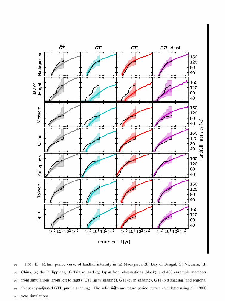
FIG. 13. Return period curve of landfall intensity in (a) Madagascar,(b) Bay of Bengal, (c) Vietnam, (d)

China, (e) the Philippines, (f) Taiwan, and (g) Japan from observations (black), and 400 ensemble members

from simulations (from left to right): GTI (gray shading), GTI (cyan shading), GTI (red shading) and regional

frequency-adjusted GTI (purple shading). The solid lines are return period curves calculated using all 12800

year simulations.

645

646

647

648

649

42

FIG. 14. Continuation of Fig. 13. (h) western Mexico, (i) Caribbean islands, (j) Gulf of Mexico, (k) Eastern

US, (l) Pacific islands, and (m) Australia.

650

651

43