An Epidemiological Approach tothe Spread of Political Third Parties

Karl Calderon1, Clara Orbe2, Azra Panjwani3, Daniel M. Romero4,Christopher Kribs-Zaleta5, Karen Rıos-Soto6

1 University of Arizona,

Department of Mathematics, Tucson, AZ2 Brown University,

Department of Applied Mathematics, Providence, RI3 University of California,

Department of Mathematics, Berkeley, Berkeley, CA4 Arizona State University,

Department of Mathematics and Statistics, Tempe, AZ5 University of Texas, Arlington,

Department of Mathematics, Arlington, TX6 Cornell University,

Department of Biometrics, Ithaca, NY

August 5, 2005

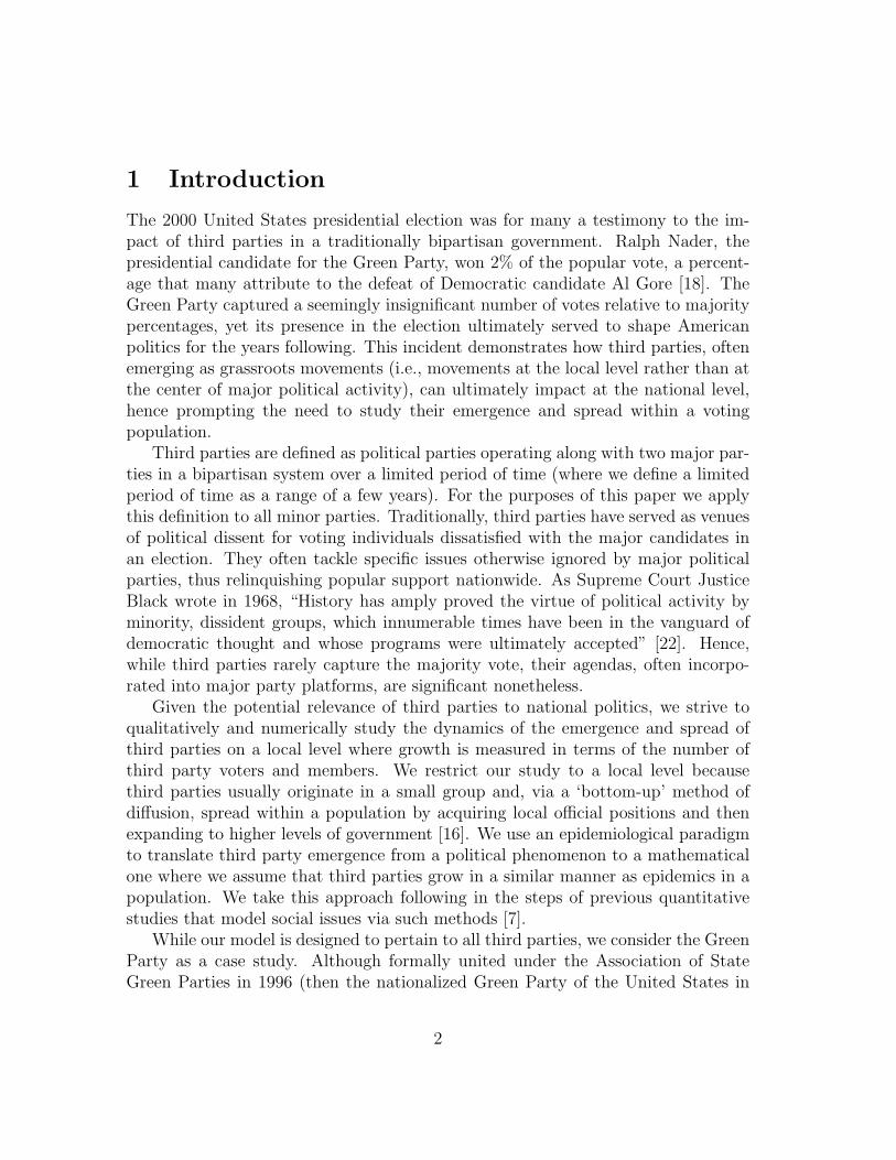
AbstractThird political parties are influential in shaping American politics. In this work we study the

spread of third parties ideologies in a voting population where we assume that party members are

more influential in recruiting new third party voters than non-member third party voters. The study

is conducted using an epidemiological model with nonlinear ordinary differential equations as applied

to a case study, the Green Party. Through the analysis of our system we obtain the party-free and

member-free equilibria as well as two endemic equilibria. We identify two threshold parameters in

our model that describe the different possible scenarios for the political parties and their spread.

Our system produces a backward bifurcation that helps identify conditions under which a third

party can thrive. We perform a sensitivity analysis to the threshold conditions in order to isolate

those parameters to which our model is most sensitive. We explore all results through deterministic

simulations and refer to data from the Green Party in the state of Pennsylvania as a case study.

1

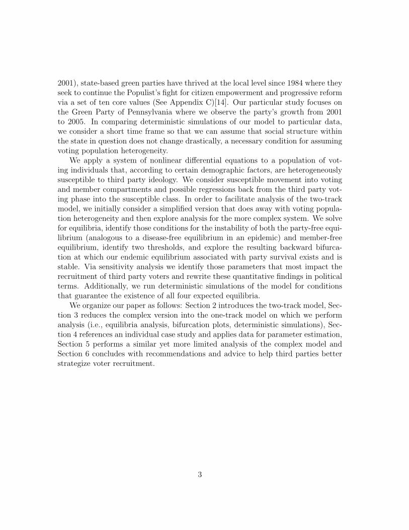
1 Introduction

The 2000 United States presidential election was for many a testimony to the im-pact of third parties in a traditionally bipartisan government. Ralph Nader, thepresidential candidate for the Green Party, won 2% of the popular vote, a percent-age that many attribute to the defeat of Democratic candidate Al Gore [18]. TheGreen Party captured a seemingly insignificant number of votes relative to majoritypercentages, yet its presence in the election ultimately served to shape Americanpolitics for the years following. This incident demonstrates how third parties, oftenemerging as grassroots movements (i.e., movements at the local level rather than atthe center of major political activity), can ultimately impact at the national level,hence prompting the need to study their emergence and spread within a votingpopulation.

Third parties are defined as political parties operating along with two major par-ties in a bipartisan system over a limited period of time (where we define a limitedperiod of time as a range of a few years). For the purposes of this paper we applythis definition to all minor parties. Traditionally, third parties have served as venuesof political dissent for voting individuals dissatisfied with the major candidates inan election. They often tackle specific issues otherwise ignored by major politicalparties, thus relinquishing popular support nationwide. As Supreme Court JusticeBlack wrote in 1968, “History has amply proved the virtue of political activity byminority, dissident groups, which innumerable times have been in the vanguard ofdemocratic thought and whose programs were ultimately accepted” [22]. Hence,while third parties rarely capture the majority vote, their agendas, often incorpo-rated into major party platforms, are significant nonetheless.

Given the potential relevance of third parties to national politics, we strive toqualitatively and numerically study the dynamics of the emergence and spread ofthird parties on a local level where growth is measured in terms of the number ofthird party voters and members. We restrict our study to a local level becausethird parties usually originate in a small group and, via a ‘bottom-up’ method ofdiffusion, spread within a population by acquiring local official positions and thenexpanding to higher levels of government [16]. We use an epidemiological paradigmto translate third party emergence from a political phenomenon to a mathematicalone where we assume that third parties grow in a similar manner as epidemics in apopulation. We take this approach following in the steps of previous quantitativestudies that model social issues via such methods [7].

While our model is designed to pertain to all third parties, we consider the GreenParty as a case study. Although formally united under the Association of StateGreen Parties in 1996 (then the nationalized Green Party of the United States in

2

2001), state-based green parties have thrived at the local level since 1984 where theyseek to continue the Populist’s fight for citizen empowerment and progressive reformvia a set of ten core values (See Appendix C)[14]. Our particular study focuses onthe Green Party of Pennsylvania where we observe the party’s growth from 2001to 2005. In comparing deterministic simulations of our model to particular data,we consider a short time frame so that we can assume that social structure withinthe state in question does not change drastically, a necessary condition for assumingvoting population heterogeneity.

We apply a system of nonlinear differential equations to a population of vot-ing individuals that, according to certain demographic factors, are heterogeneouslysusceptible to third party ideology. We consider susceptible movement into votingand member compartments and possible regressions back from the third party vot-ing phase into the susceptible class. In order to facilitate analysis of the two-trackmodel, we initially consider a simplified version that does away with voting popula-tion heterogeneity and then explore analysis for the more complex system. We solvefor equilibria, identify those conditions for the instability of both the party-free equi-librium (analogous to a disease-free equilibrium in an epidemic) and member-freeequilibrium, identify two thresholds, and explore the resulting backward bifurca-tion at which our endemic equilibrium associated with party survival exists and isstable. Via sensitivity analysis we identify those parameters that most impact therecruitment of third party voters and rewrite these quantitative findings in politicalterms. Additionally, we run deterministic simulations of the model for conditionsthat guarantee the existence of all four expected equilibria.

We organize our paper as follows: Section 2 introduces the two-track model, Sec-tion 3 reduces the complex version into the one-track model on which we performanalysis (i.e., equilibria analysis, bifurcation plots, deterministic simulations), Sec-tion 4 references an individual case study and applies data for parameter estimation,Section 5 performs a similar yet more limited analysis of the complex model andSection 6 concludes with recommendations and advice to help third parties betterstrategize voter recruitment.

3

1.1 A Population Model for the Spread of a Third Party

Our model considers a population of all voters, N , divided into two classes or sub-populations whose susceptibility to third party ideology is based on the followingdemographic factors: education, socioeconomic status, race, gender, age, politicalorientation and professional occupation. We assume that individuals do not movefrom one susceptible class to the other. See Assumption 3 in Section 2.3 (hereonrefer to all assumptions in Section 2.3). Inherently, certain demographic factors,labelled as high affinity, make an individual more likely to subscribe to a third party’sideology that, as detailed in Assumption 4, targets a more specific audience thanalternative majority agendas. For this reason we consider population heterogeneityvital to this study. When an individual enters the voting system that person, dueto his/her characteristic demographic factors, is more statistically inclined to vote acertain way. For example, a progressive environmental activist is statistically morelikely to agree and vote for the Green Party agenda, that stresses communal basedeconomics, local government, and gender and racial equity, than a conservativecorporate executive whose economic philosophy directly conflicts with that of theGreen Party.

We apply the following method of dividing the entering voting population intotwo susceptible classes: if an individual has more high affinity factors than low affin-ity factors then that person directly enters the high affinity class and similarly forlow affinity susceptibles. We define high affinity factors as features of the individualbased on his/her demographic profile that make him/her more inclined to vote forthe third party; conversely, low affinity factors make the individual less statisticallylikely to subscribe to the party’s platform. Each party has its own agenda thatappeals to certain sectors of the voting population. Hence different parties targetvoting populations that are more inclined to subscribe to their ideology. While oneparty, for example, may target individuals from a certain educational backgroundthat we, in our model, label as high affinity and that other parties may overlook, allparties nonetheless recognize that education factors into an individual’s likelihoodto support or refute that party’s platform. It is true that individuals from variedbackgrounds comprise the main parties yet, when dealing with the specific agendasof third parties that do not strive to sway the majority vote, we assume that thirdparties appeal to individuals of certain demographic backgrounds more than others.See Assumption 4. Therefore, we account for the aforementioned standard set of de-mographic factors that parties look at when spreading their ideologies. In our paperwe apply our model to an individual case study of the Green Party of Pennsylvania;however, the same methodology of distinguishing susceptibles can be applied to allthird parties.

4

All voters enter the voting system either to the low affinity, L, or high affin-ity, H, susceptible class. Our Susceptible/Infected-based model then considers twosusceptible and three infected classes, VH , VL, and M , third party voters from thehigh affinity class, third party voters from the low affinity class and party membersrespectively. We define party members as voters of the third party who pay dues tothe party; often such members officiate, volunteer and actively campaign for voterrecruitment. We apply epidemiological terminology, specifically ‘infectious’, whenreferring to susceptibles who transition to the voting and, possibly, member classes.In biological terms, VH and VL correspond to voters of a lower degree of infectionand individuals of the M class are voters infected to a higher degree. Once an indi-vidual is susceptible he/she can become ‘infected’ (either VH or VL) through directcontact with the VH , VL, and M classes. We do not consider a linear term weighingthe influence of media coverage from the third party (i.e., secondary contact factors)in the forward transition from both susceptible classes to third party voting classes.See Assumption 5. Instead, we focus on the nonlinear terms considering the effectsof voters from the VH , VL, and M classes where voters from VH and VL bear an equalinfluence β1 (from H to VH) and β2 (from L to VL) in third party voter recruitment;members from M influence susceptibles at a rate proportional to voter influence,embodied in the multiplicative factors αβ1 and αβ2. See Assumption 6.

We consider the transition back from the third party voting to the susceptibleclasses that involves the linear terms, ε1VH and ε2VL, and nonlinear terms, φ1(τH +L)VH

Nand φ2(τL + H)VL

N, contributions by secondary contacts with the opposition

(i.e., media from well-funded majority voters) and direct contact with the susceptibleclasses respectively. See Assumption 7. Similar to α in the forward transition, wedesignate τ as the augmentation factor. Therefore, in regressing back from VH toH, τH represents the greater influence that H individuals exert on voters from VH

than susceptibles from L, the lower affinity class (similar reasoning applies to theVL to L transition). See Assumption 10.

Once voting for the third party, individuals can become party members. Theyenter this higher state of infection via the nonlinear terms γVH

MN

and γVLMN

, wherewe only consider the effects of party membership on bringing about this transitionembodied in the general parameter γ. See Assumption 5. Given that we are studyingthe spread of the party we assume that party members stay in M and do not regressto other classes. See Assumption 9.

Finally, we consider natural exits from all classes as a result of death or moving.The sum of the equations of the model, for both the complex and simple versions,dNdt

= 0, verifies that our population stays constant, a safe assumption by whichthe number of people entering the voting system (i.e., coming of age, moving in)counterbalances the number of people leaving the system (i.e., dying, moving out).

5

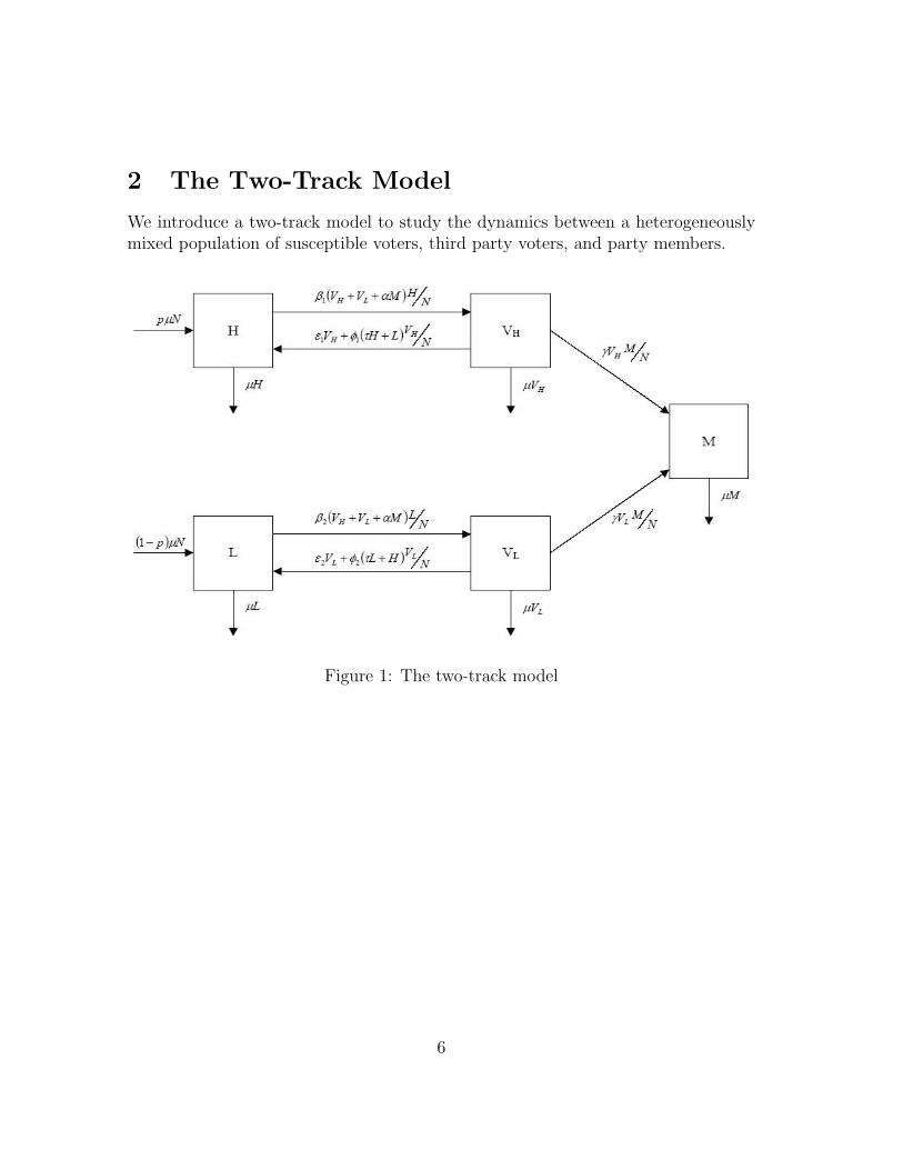
2 The Two-Track Model

We introduce a two-track model to study the dynamics between a heterogeneouslymixed population of susceptible voters, third party voters, and party members.

Figure 1: The two-track model

6

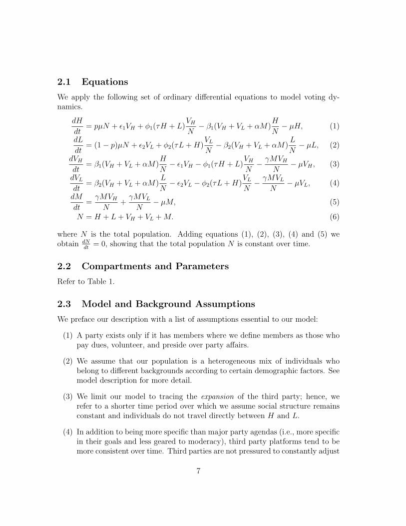
2.1 Equations

We apply the following set of ordinary differential equations to model voting dy-namics.

dH

dt= pµN + ε1VH + φ1(τH + L)

VH

N− β1(VH + VL + αM)

H

N− µH, (1)

dL

dt= (1− p)µN + ε2VL + φ2(τL + H)

VL

N− β2(VH + VL + αM)

L

N− µL, (2)

dVH

dt= β1(VH + VL + αM)

H

N− ε1VH − φ1(τH + L)

VH

N− γMVH

N− µVH , (3)

dVL

dt= β2(VH + VL + αM)

L

N− ε2VL − φ2(τL + H)

VL

N− γMVL

N− µVL, (4)

dM

dt=

γMVH

N+

γMVL

N− µM, (5)

N = H + L + VH + VL + M. (6)

where N is the total population. Adding equations (1), (2), (3), (4) and (5) weobtain dN

dt= 0, showing that the total population N is constant over time.

2.2 Compartments and Parameters

Refer to Table 1.

2.3 Model and Background Assumptions

We preface our description with a list of assumptions essential to our model:

(1) A party exists only if it has members where we define members as those whopay dues, volunteer, and preside over party affairs.

(2) We assume that our population is a heterogeneous mix of individuals whobelong to different backgrounds according to certain demographic factors. Seemodel description for more detail.

(3) We limit our model to tracing the expansion of the third party; hence, werefer to a shorter time period over which we assume social structure remainsconstant and individuals do not travel directly between H and L.

(4) In addition to being more specific than major party agendas (i.e., more specificin their goals and less geared to moderacy), third party platforms tend to bemore consistent over time. Third parties are not pressured to constantly adjust

7

Table of Parameters and CompartmentsH high affinity susceptibles (i.e. voters highly susceptible to third party ideology)L low affinity susceptibles (i.e. voters barely susceptible to third party ideology)VH third party voting individuals deriving from HVL third party voter individuals deriving from SM third party members (i.e. party officials, donors, volunteers)p proportion of the voting population N entering Hβ1 peer driven recruitment rate of H into VH by individuals in VH , VL and Mα factor by which the recruitment rate of H and L into VH and VL by individuals

in M exceeds the recruitment rate by individuals in VH and VL

ε1 linear recruitment rate of VH back into Hvia secondary contacts (i.e., media and campaigning from opposing parties)

φ1 recruitment rate of VH into Hby direct contact with individuals in the opposition classes (i.e., individuals in H and L)

β2 peer driven recruitment rate of L intoVL by individuals in VL, VH , and M (analogous to β1).

τ factor by which the recruitment rate of VH and VL

by members of the same susceptibleclass exceeds the recruitment rate by susceptibles of the other class

ε2 linear recruitment rate of VL back into Lvia secondary contacts (i.e., media and campaigning from opposing parties)

φ2 recruitment rate of VL into L by direct contact with individualsin the opposition classes (i.e., individuals in H and L)

γ recruitment rate of VH and VL into M by individuals in Mµ rate at which individuals enter or leave the voting system

Table 1: Compartments and parameters of the two-track model.

to the shifting demands of the populace since they do not seek the majorityvote. Consequently, they do not target the majority voting population.

(5) We assume that third parties, due to a lack of funding and resulting lack ofmedia exposure to the general population, spread mainly via primary contactsamong susceptibles, H and L, third party voters, VH and VL, and members,M , at the rates β and αβ respectively. We define such direct interaction aspersonal meetings, phone conversations, and personally addressed emails.

8

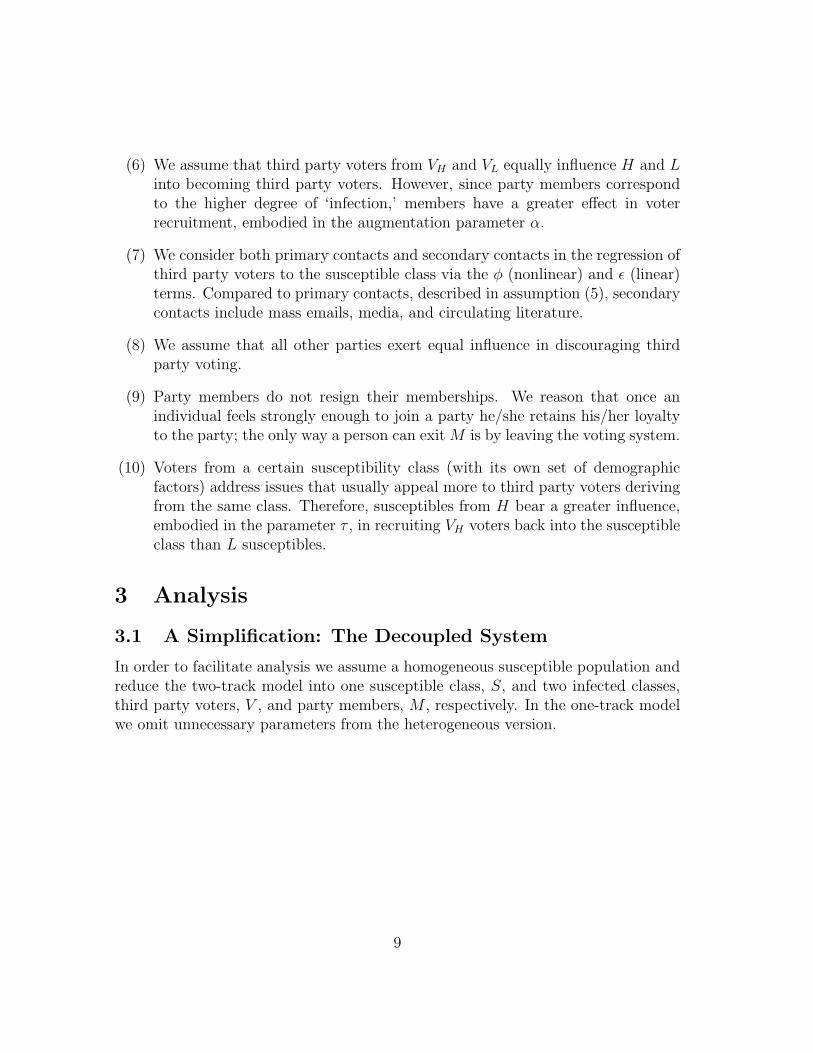
(6) We assume that third party voters from VH and VL equally influence H and Linto becoming third party voters. However, since party members correspondto the higher degree of ‘infection,’ members have a greater effect in voterrecruitment, embodied in the augmentation parameter α.

(7) We consider both primary contacts and secondary contacts in the regression ofthird party voters to the susceptible class via the φ (nonlinear) and ε (linear)terms. Compared to primary contacts, described in assumption (5), secondarycontacts include mass emails, media, and circulating literature.

(8) We assume that all other parties exert equal influence in discouraging thirdparty voting.

(9) Party members do not resign their memberships. We reason that once anindividual feels strongly enough to join a party he/she retains his/her loyaltyto the party; the only way a person can exit M is by leaving the voting system.

(10) Voters from a certain susceptibility class (with its own set of demographicfactors) address issues that usually appeal more to third party voters derivingfrom the same class. Therefore, susceptibles from H bear a greater influence,embodied in the parameter τ , in recruiting VH voters back into the susceptibleclass than L susceptibles.

3 Analysis

3.1 A Simplification: The Decoupled System

In order to facilitate analysis we assume a homogeneous susceptible population andreduce the two-track model into one susceptible class, S, and two infected classes,third party voters, V , and party members, M , respectively. In the one-track modelwe omit unnecessary parameters from the heterogeneous version.

9

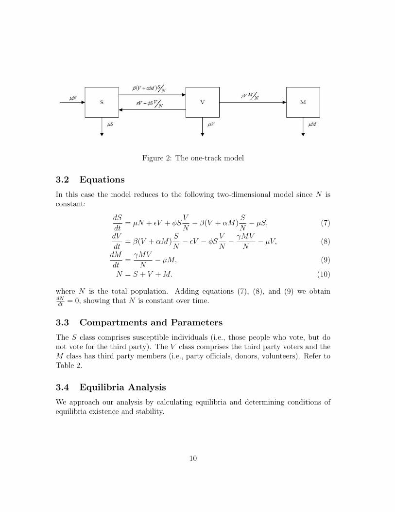
Figure 2: The one-track model

3.2 Equations

In this case the model reduces to the following two-dimensional model since N isconstant:

dS

dt= µN + εV + φS

V

N− β(V + αM)

S

N− µS, (7)

dV

dt= β(V + αM)

S

N− εV − φS

V

N− γMV

N− µV, (8)

dM

dt=

γMV

N− µM, (9)

N = S + V + M. (10)

where N is the total population. Adding equations (7), (8), and (9) we obtaindNdt

= 0, showing that N is constant over time.

3.3 Compartments and Parameters

The S class comprises susceptible individuals (i.e., those people who vote, but donot vote for the third party). The V class comprises the third party voters and theM class has third party members (i.e., party officials, donors, volunteers). Refer toTable 2.

3.4 Equilibria Analysis

We approach our analysis by calculating equilibria and determining conditions ofequilibria existence and stability.

10

β peer driven recruitment rate of S into V by third party voters and membersε recruitment rate of V back into S

via secondary contacts (i.e., media and campaigning from opposing parties)φ recruitment rate of V into S by direct contact with susceptiblesα factor by which the recruitment rate of S into V by

third party members exceeds the recruitment rate by individuals in Vγ recruitment rate of V into M by third party membersµ rate at which individuals enter or leave the voting system

Table 2: Parameters of the one-track model.

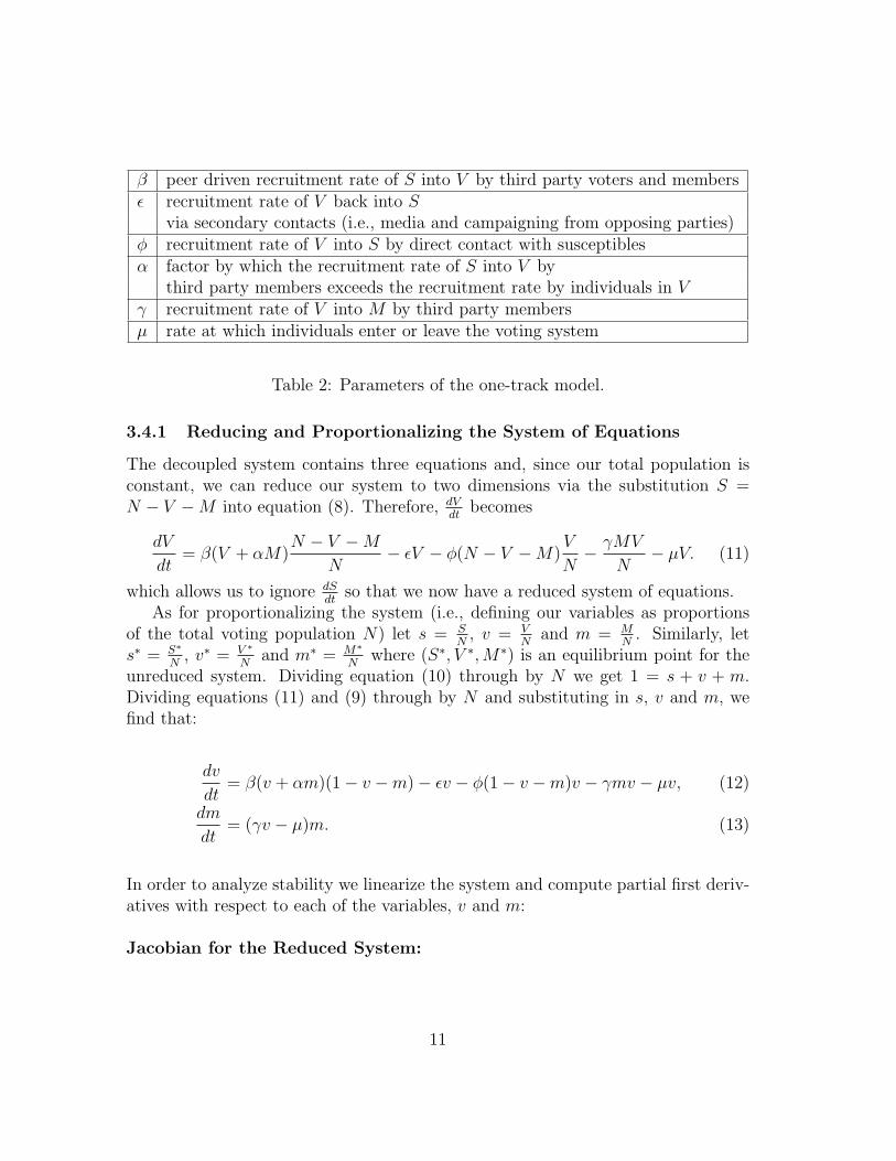
3.4.1 Reducing and Proportionalizing the System of Equations

The decoupled system contains three equations and, since our total population isconstant, we can reduce our system to two dimensions via the substitution S =N − V −M into equation (8). Therefore, dV

dtbecomes

dV

dt= β(V + αM)

N − V −M

N− εV − φ(N − V −M)

V

N− γMV

N− µV. (11)

which allows us to ignore dSdt

so that we now have a reduced system of equations.As for proportionalizing the system (i.e., defining our variables as proportions

of the total voting population N) let s = SN

, v = VN

and m = MN

. Similarly, lets∗ = S∗

N, v∗ = V ∗

Nand m∗ = M∗

Nwhere (S∗, V ∗, M∗) is an equilibrium point for the

unreduced system. Dividing equation (10) through by N we get 1 = s + v + m.Dividing equations (11) and (9) through by N and substituting in s, v and m, wefind that:

dv

dt= β(v + αm)(1− v −m)− εv − φ(1− v −m)v − γmv − µv, (12)

dm

dt= (γv − µ)m. (13)

In order to analyze stability we linearize the system and compute partial first deriv-atives with respect to each of the variables, v and m:

Jacobian for the Reduced System:

11

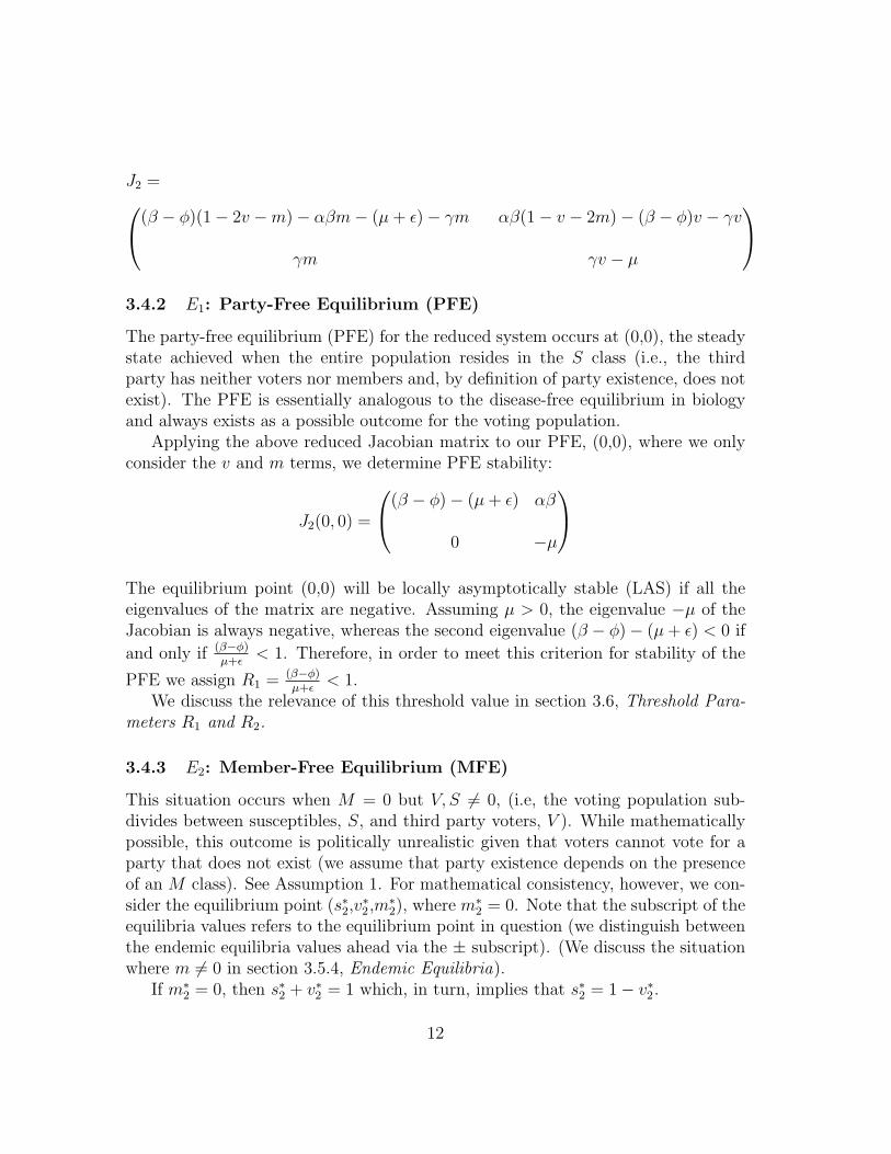
J2 =(β − φ)(1− 2v −m)− αβm− (µ + ε)− γm αβ(1− v − 2m)− (β − φ)v − γv

γm γv − µ

3.4.2 E1: Party-Free Equilibrium (PFE)

The party-free equilibrium (PFE) for the reduced system occurs at (0,0), the steadystate achieved when the entire population resides in the S class (i.e., the thirdparty has neither voters nor members and, by definition of party existence, does notexist). The PFE is essentially analogous to the disease-free equilibrium in biologyand always exists as a possible outcome for the voting population.

Applying the above reduced Jacobian matrix to our PFE, (0,0), where we onlyconsider the v and m terms, we determine PFE stability:

J2(0, 0) =

(β − φ)− (µ + ε) αβ

0 −µ

The equilibrium point (0,0) will be locally asymptotically stable (LAS) if all theeigenvalues of the matrix are negative. Assuming µ > 0, the eigenvalue −µ of theJacobian is always negative, whereas the second eigenvalue (β − φ)− (µ + ε) < 0 if

and only if (β−φ)µ+ε

< 1. Therefore, in order to meet this criterion for stability of the

PFE we assign R1 = (β−φ)µ+ε

< 1.We discuss the relevance of this threshold value in section 3.6, Threshold Para-

meters R1 and R2.

3.4.3 E2: Member-Free Equilibrium (MFE)

This situation occurs when M = 0 but V, S 6= 0, (i.e, the voting population sub-divides between susceptibles, S, and third party voters, V ). While mathematicallypossible, this outcome is politically unrealistic given that voters cannot vote for aparty that does not exist (we assume that party existence depends on the presenceof an M class). See Assumption 1. For mathematical consistency, however, we con-sider the equilibrium point (s∗2,v

∗2,m

∗2), where m∗

2 = 0. Note that the subscript of theequilibria values refers to the equilibrium point in question (we distinguish betweenthe endemic equilibria values ahead via the ± subscript). (We discuss the situationwhere m 6= 0 in section 3.5.4, Endemic Equilibria).

If m∗2 = 0, then s∗2 + v∗2 = 1 which, in turn, implies that s∗2 = 1− v∗2.

12

Rearranging equation (12) of the decoupled system together while substitutingin m∗

2 = 0 and v∗2 we have:

(β − φ)v∗22 + (µ + ε + φ− β)v∗2 = 0 (14)

This implies that either v∗2 = 0 or (β − φ)v∗2 = β − (µ + ε + φ).We consider the situation where v∗2 6= 0, solve for v∗2 and simplify the results as

follows:

v∗2 = 1− µ + ε

β − φ= 1− 1

R1

where v∗2 retains political value only if R1 > 1 or else v∗2 < 0 which is a contradictiongiven that 0 ≤ 1 and is a politically irrelevant number of individuals.

Similarly we solve for s∗2 and obtain s∗2 = 1− v∗2 = µ+εβ−φ

= 1R1

which makes sense

politically only if β > φ (i.e, s2 > 0). From solving for s∗2 and v∗2 above, we expressour member-free equilibrium as E2 = ( µ+ε

β−φ, 1− µ+ε

β−φ, 0).

Expressed in terms of R1, the MFE is ( 1R1

, 1 − 1R1

, 0) and exists if and only ifR1 > 1, since ignoring this condition leads to an otherwise negative third partyvoting population. If R1 > 1, then 1

R1< 1 (i.e., the entire population does not

reside in the susceptible class). This implies that the population has moved out ofS into the V and M classes. Since M = 0, the left over proportion (i.e., 1 − 1

R1)

resides in V .The above situation makes mathematical sense but not political sense since par-

ties, by our original assumption, do not exist without members and in this member-free case we deal with voters that vote for a non-existent party.

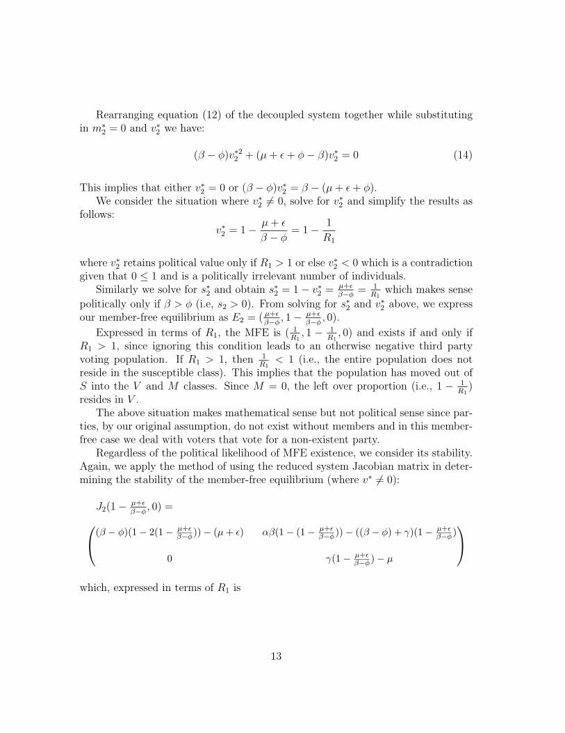
Regardless of the political likelihood of MFE existence, we consider its stability.Again, we apply the method of using the reduced system Jacobian matrix in deter-mining the stability of the member-free equilibrium (where v∗ 6= 0):

J2(1− µ+εβ−φ

, 0) =(β − φ)(1− 2(1− µ+εβ−φ))− (µ + ε) αβ(1− (1− µ+ε

β−φ))− ((β − φ) + γ)(1− µ+εβ−φ)

0 γ(1− µ+εβ−φ)− µ

which, expressed in terms of R1 is

13

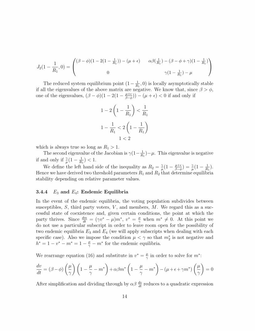
J2(1−1

R1

, 0) =

(β − φ)(1− 2(1− 1R1

))− (µ + ε) αβ( 1R1

)− (β − φ + γ)(1− 1R1

)

0 γ(1− 1R1

)− µ

The reduced system equilibrium point (1− 1

R1, 0) is locally asymptotically stable

if all the eigenvalues of the above matrix are negative. We know that, since β > φ,one of the eigenvalues, (β − φ)(1− 2(1− µ+ε

β−φ))− (µ + ε) < 0 if and only if

1− 2

(1− 1

R1

)<

1

R1

1− 1

R1

< 2

(1− 1

R1

)1 < 2

which is always true so long as R1 > 1.The second eigenvalue of the Jacobian is γ(1− 1

R1)−µ. This eigenvalue is negative

if and only if γµ(1− 1

R1) < 1.

We define the left hand side of the inequality as R2 = γµ(1− µ+ε

β−φ) = γ

µ(1− 1

R1).

Hence we have derived two threshold parameters R1 and R2 that determine equilibriastability depending on relative parameter values.

3.4.4 E3 and E4: Endemic Equilibria

In the event of the endemic equilibria, the voting population subdivides betweensusceptibles, S, third party voters, V , and members, M . We regard this as a suc-cessful state of coexistence and, given certain conditions, the point at which theparty thrives. Since dm

dt= (γv∗ − µ)m∗, v∗ = µ

γwhen m∗ 6= 0. At this point we

do not use a particular subscript in order to leave room open for the possibility oftwo endemic equilibria E3 and E4 (we will apply subscripts when dealing with eachspecific case). Also we impose the condition µ < γ so that m∗

2 is not negative andh∗ = 1− v∗ −m∗ = 1− µ

γ−m∗ for the endemic equilibria.

We rearrange equation (16) and substitute in v∗ = µγ

in order to solve for m∗:

dv

dt= (β−φ)

(µ

γ

)(1− µ

γ−m∗

)+αβm∗

(1− µ

γ−m∗

)− (µ+ ε+γm∗)

(µ

γ

)= 0

After simplification and dividing through by αβ dvdt

reduces to a quadratic expression

14

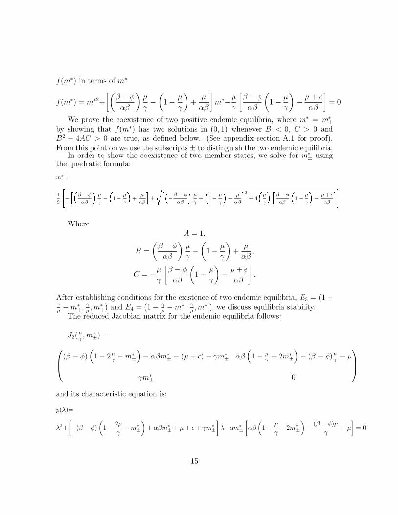
f(m∗) in terms of m∗

f(m∗) = m∗2+

[(β − φ

αβ

)µ

γ−(

1− µ

γ

)+

µ

αβ

]m∗−µ

γ

[β − φ

αβ

(1− µ

γ

)− µ + ε

αβ

]= 0

We prove the coexistence of two positive endemic equilibria, where m∗ = m∗±

by showing that f(m∗) has two solutions in (0, 1) whenever B < 0, C > 0 andB2 − 4AC > 0 are true, as defined below. (See appendix section A.1 for proof).From this point on we use the subscripts ± to distinguish the two endemic equilibria.

In order to show the coexistence of two member states, we solve for m∗± using

the quadratic formula:

m∗± =

1

2

24− ��β − φ

αβ

�µ

γ−�

1−µ

γ

�+

µ

αβ

�±

s��−

β − φ

αβ

�µ

γ+

�1−

µ

γ

�−

µ

αβ

�2+ 4

�µ

γ

��β − φ

αβ

�1−

µ

γ

�−

µ + ε

αβ

�35

WhereA = 1,

B =

(β − φ

αβ

)µ

γ−(

1− µ

γ

)+

µ

αβ,

C = −µ

γ

[β − φ

αβ

(1− µ

γ

)− µ + ε

αβ

].

After establishing conditions for the existence of two endemic equilibria, E3 = (1−γµ−m∗

+, γµ, m∗

+) and E4 = (1− γµ−m∗

−, γµ, m∗

−), we discuss equilibria stability.The reduced Jacobian matrix for the endemic equilibria follows:

J2(µγ, m∗

±) =(β − φ)(1− 2µ

γ−m∗

±

)− αβm∗

± − (µ + ε)− γm∗± αβ

(1− µ

γ− 2m∗

±

)− (β − φ)µ

γ− µ

γm∗± 0

and its characteristic equation is:

p(λ)=

λ2+[−(β − φ)

(1− 2µ

γ−m∗

±

)+ αβm∗

± + µ + ε + γm∗±

]λ−αm∗

±

[αβ

(1− µ

γ− 2m∗

±

)− (β − φ)µ

γ− µ

]= 0

15

The solutions of the characteristic equation are the eigenvalues of J2(µγ, m∗

±), andthe stability of the endemic equilibria depends on the signs of the real parts of theeigenvalues. If the real parts of both eigenvalues are negative then we conclude thatthe endemic equilibrium in question is locally asymptotically stable. Based on thiscriterion, we find that E3 is always LAS when it exists while E4 is never LAS whenit exists. (See appendix A.2 for details).

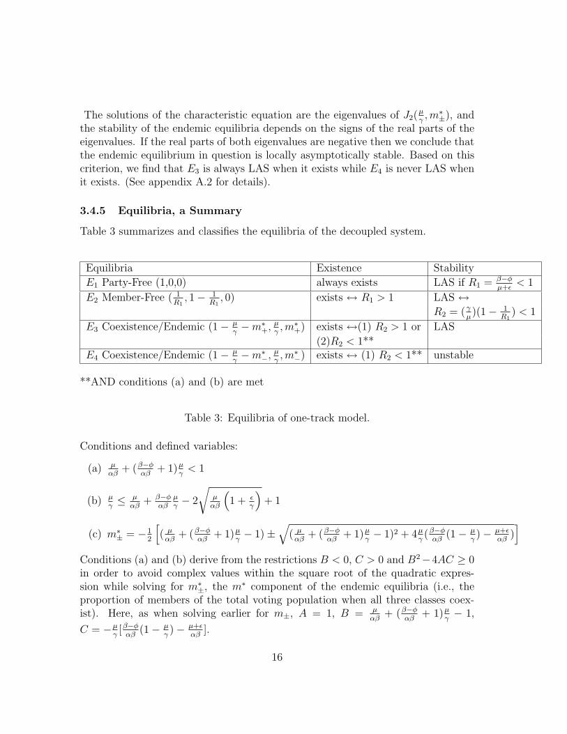
3.4.5 Equilibria, a Summary

Table 3 summarizes and classifies the equilibria of the decoupled system.

Equilibria Existence Stability

E1 Party-Free (1,0,0) always exists LAS if R1 = β−φµ+ε

< 1

E2 Member-Free ( 1R1

, 1− 1R1

, 0) exists ↔ R1 > 1 LAS ↔R2 = ( γ

µ)(1− 1

R1) < 1

E3 Coexistence/Endemic (1− µγ−m∗

+, µγ, m∗

+) exists ↔(1) R2 > 1 or LAS

(2)R2 < 1**E4 Coexistence/Endemic (1− µ

γ−m∗

−, µγ, m∗

−) exists ↔ (1) R2 < 1** unstable

**AND conditions (a) and (b) are met

Table 3: Equilibria of one-track model.

Conditions and defined variables:

(a) µαβ

+ (β−φαβ

+ 1)µγ

< 1

(b) µγ≤ µ

αβ+ β−φ

αβµγ− 2

õ

αβ

(1 + ε

γ

)+ 1

(c) m∗± = −1

2

[( µ

αβ+ (β−φ

αβ+ 1)µ

γ− 1)±

√( µ

αβ+ (β−φ

αβ+ 1)µ

γ− 1)2 + 4µ

γ(β−φ

αβ(1− µ

γ)− µ+ε

αβ)]

Conditions (a) and (b) derive from the restrictions B < 0, C > 0 and B2−4AC ≥ 0in order to avoid complex values within the square root of the quadratic expres-sion while solving for m∗

±, the m∗ component of the endemic equilibria (i.e., theproportion of members of the total voting population when all three classes coex-ist). Here, as when solving earlier for m±, A = 1, B = µ

αβ+ (β−φ

αβ+ 1)µ

γ− 1,

C = −µγ[β−φ

αβ(1− µ

γ)− µ+ε

αβ].

16

3.5 Threshold Parameters, R1 and R2

Our system contains two local thresholds or tipping points where population out-comes, measured as S, V , and M , depend on parameter values. By tipping point werefer to the sociological term that describes the point at which a stable phenomenonturns into a crisis, which in a political context, corresponds to the extreme statesof the party: death and growth [11]. In the context of our model, for example, theparty can very well die out up until parameter conditions reach R1 = 1 after whichpoint the third party voting and member classes gain individuals. We distinguishbetween the aforementioned thresholds, R1 and R2, by analyzing them qualitativelyin a political context.

3.5.1 Interpreting R1 and R2

1. R1 = β−φµ+ε

: We interpret this threshold value as the net peer pressure, β − φ,

on susceptibles by individuals of V multiplied by the average time, 1µ+ε

, spentin the voting class V . The numerator couples those factors that bear a directinfluence (i.e., personal contacts) on the transition between S and V , whereasindirect factors (i.e., secondary contacts such as opposition media and naturalexits from the system), µ and ε, comprise the denominator. R1 denotes theaverage number of susceptibles an individual in V or M would convert ifdropped in a homogeneous population of susceptibles.

2. R2 = ( γµ)(1 − 1

R1): We interpret this threshold value as the product of the

average time in the voting system, 1µ, the rate of recruiting voters from V into

M via influence from party members, γ, and the proportion of the populationN in V , (1− 1

R1). Similar to R1, R2 measures the average number of V to M

conversions per individual in the M class; hence, R2 is essentially a measureof how effective party members are in recruiting third party voters to becomemembers once there are enough individuals in V .

3.5.2 An Analysis of the Various Conditions of R1 and R2

(i) When R1 < 1 the member-free equilibrium, E2, does not exist since V < 0, anunrealistic population. Rather, under such conditions, E1, the PFE, not onlyexists but is locally asymptotically stable and the party dies out. However,under certain initial conditions (i.e., a substantial number of M individuals)we note that the party can survive even when R1 < 1 since, for R2 = γ

µ(1− 1

R1),

R1 < 1 also implies R2 < 0. (See related explanation (iii)).

17

(ii) When R1 > 1 each individual in V and M is converting more than one personin S into V , thus allowing the V class to thrive. In other words, while R1 > 1renders the PFE unstable it also implies the existence and stability of the MFE(given that R2 < 1) which, as described earlier, does not exist in the politicalworld since a party cannot exist without members. However, as with the casewhen R1 < 1, we can ensure the coexistence of the S, V and M classes whenR1 > 1 under sufficient initial conditions.

(iii) R2 < 0 occurs when R1 < 1 due to the special relationship between R2 and R1

where R2 = γµ(1− 1

R1); such a relationship denotes the existence of a negative

voting population in the MFE (i.e., no real population in the V class). SinceR2 signifies the conversion of V to M , R2 < 0 implies that M is converting anegative or non-existent V population into the M class, which initially does notmake sense in a political context. R2 < 0 seems to correspond to the stabilityof either the PFE or to the existence of a state where we have individuals Mand S and a non-existent or negative V class. However, R2 < 0 can still leadto the stable endemic equilibrium E3 via a backward bifurcation if there existsa sufficient initial number of individuals in M .

(iv) The condition R2 < 1 guarantees local asymptotic stability of the member-freeequilibrium, MFE. For this reason, the condition is not typically conducive toparty growth but, as we mentioned before, R2 < 1 may imply the coexistenceand stability of E3. This suggests that R2 is the more important of the thresh-old transitions in political terms since it is primarily concerned with the V toM transition where M individuals are more influential in third party voterrecruitment by the factor α.

(v) The condition R2 > 1 explains the case where the V and M classes grow byrecruiting members from the S and V populations respectively. In other wordsthis condition guarantees that the larger endemic equilibrium exists withoutthe additional conditions (a) and (b) imposed by the quadratic expression ofm∗

±. In a biological analog, this condition describes how M successfully invadesboth the S and V classes.

3.6 Simulations

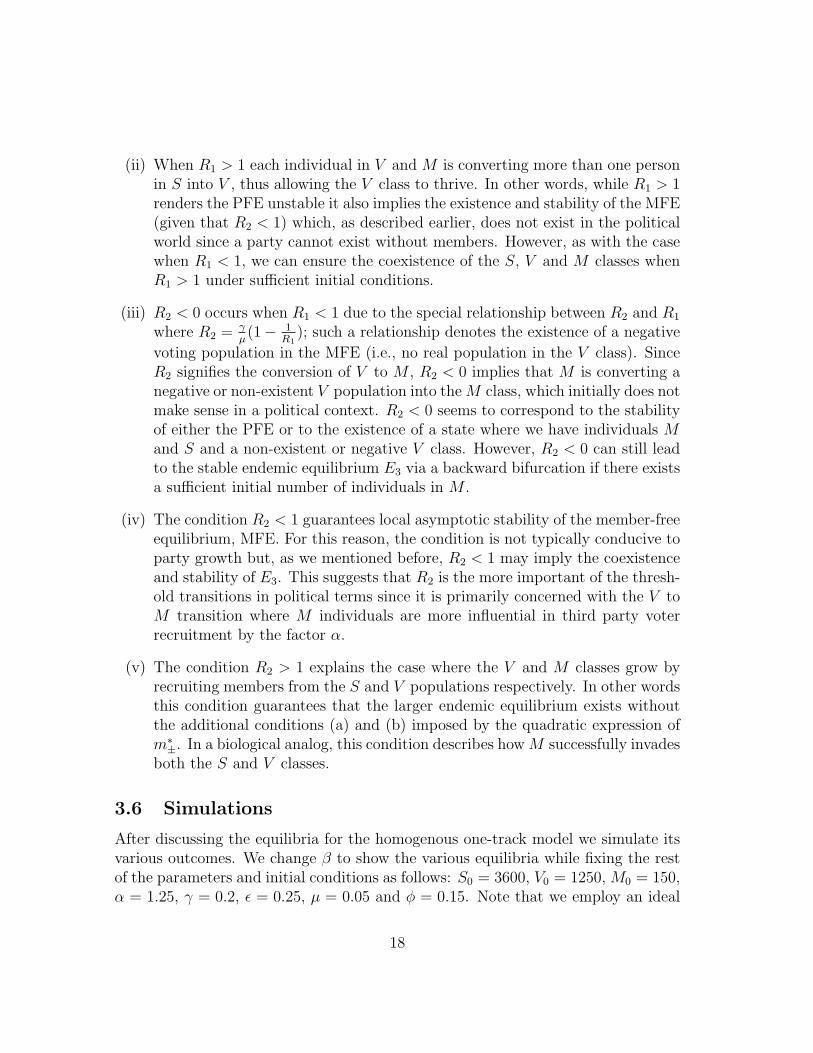
After discussing the equilibria for the homogenous one-track model we simulate itsvarious outcomes. We change β to show the various equilibria while fixing the restof the parameters and initial conditions as follows: S0 = 3600, V0 = 1250, M0 = 150,α = 1.25, γ = 0.2, ε = 0.25, µ = 0.05 and φ = 0.15. Note that we employ an ideal

18

set of parameters that we retain for the bifurcation plots in section 3.7.

Figure 3: (a) β = 0.44. (b) β = 0.49.

Figure 3(a) shows the system approaching the party-free equilibrium (E1) forβ = 0.44. For this scenario, all individuals eventually return to S and the thirdparty has neither voters nor members.

Figure 3(b) shows the system approaching the member-free equilibrium (E2) forβ = 0.49. In this case, there are no third party members and all individuals end upin either S or in V .

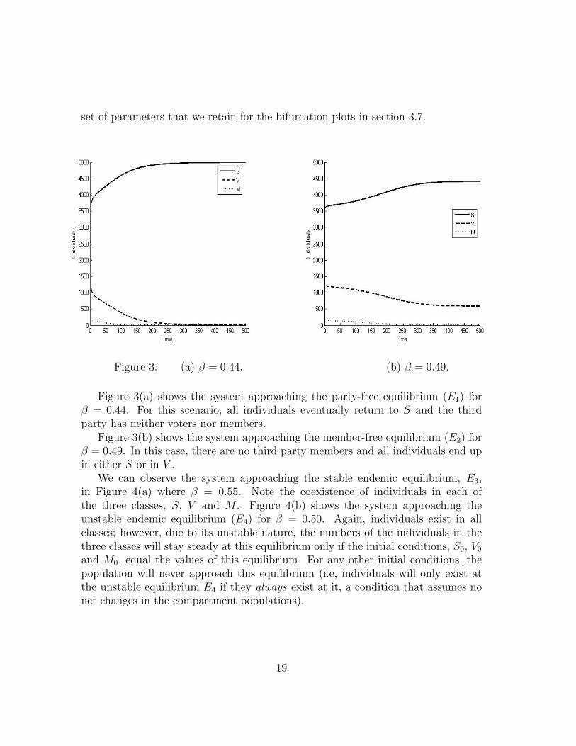
We can observe the system approaching the stable endemic equilibrium, E3,in Figure 4(a) where β = 0.55. Note the coexistence of individuals in each ofthe three classes, S, V and M . Figure 4(b) shows the system approaching theunstable endemic equilibrium (E4) for β = 0.50. Again, individuals exist in allclasses; however, due to its unstable nature, the numbers of the individuals in thethree classes will stay steady at this equilibrium only if the initial conditions, S0, V0

and M0, equal the values of this equilibrium. For any other initial conditions, thepopulation will never approach this equilibrium (i.e, individuals will only exist atthe unstable equilibrium E4 if they always exist at it, a condition that assumes nonet changes in the compartment populations).

19

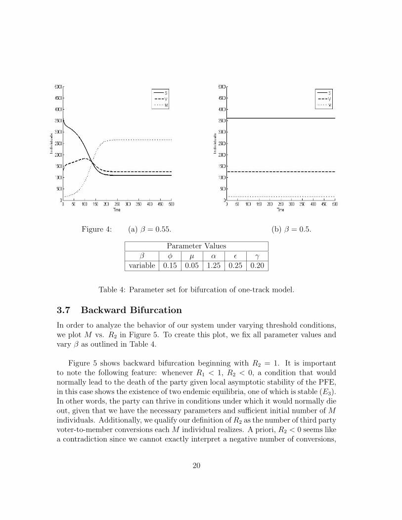
Figure 4: (a) β = 0.55. (b) β = 0.5.

Parameter Valuesβ φ µ α ε γ

variable 0.15 0.05 1.25 0.25 0.20

Table 4: Parameter set for bifurcation of one-track model.

3.7 Backward Bifurcation

In order to analyze the behavior of our system under varying threshold conditions,we plot M vs. R2 in Figure 5. To create this plot, we fix all parameter values andvary β as outlined in Table 4.

Figure 5 shows backward bifurcation beginning with R2 = 1. It is importantto note the following feature: whenever R1 < 1, R2 < 0, a condition that wouldnormally lead to the death of the party given local asymptotic stability of the PFE,in this case shows the existence of two endemic equilibria, one of which is stable (E3).In other words, the party can thrive in conditions under which it would normally dieout, given that we have the necessary parameters and sufficient initial number of Mindividuals. Additionally, we qualify our definition of R2 as the number of third partyvoter-to-member conversions each M individual realizes. A priori, R2 < 0 seems likea contradiction since we cannot exactly interpret a negative number of conversions,

20

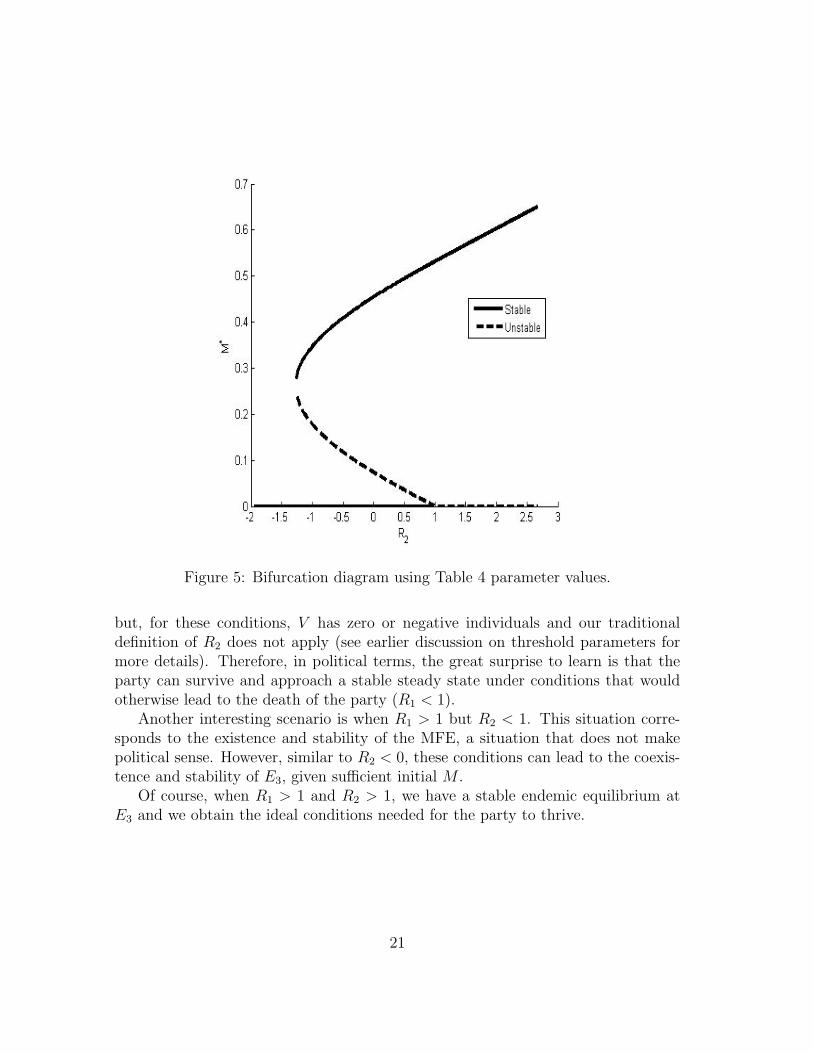
Figure 5: Bifurcation diagram using Table 4 parameter values.

but, for these conditions, V has zero or negative individuals and our traditionaldefinition of R2 does not apply (see earlier discussion on threshold parameters formore details). Therefore, in political terms, the great surprise to learn is that theparty can survive and approach a stable steady state under conditions that wouldotherwise lead to the death of the party (R1 < 1).

Another interesting scenario is when R1 > 1 but R2 < 1. This situation corre-sponds to the existence and stability of the MFE, a situation that does not makepolitical sense. However, similar to R2 < 0, these conditions can lead to the coexis-tence and stability of E3, given sufficient initial M .

Of course, when R1 > 1 and R2 > 1, we have a stable endemic equilibrium atE3 and we obtain the ideal conditions needed for the party to thrive.

21

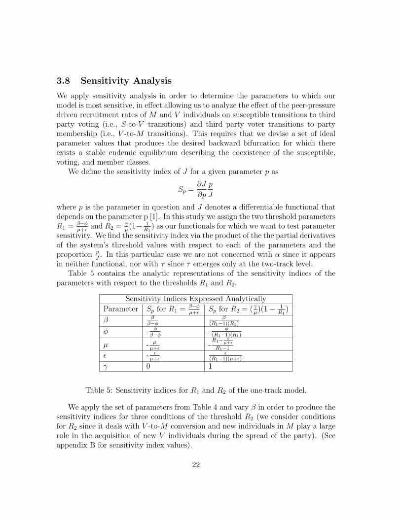
3.8 Sensitivity Analysis

We apply sensitivity analysis in order to determine the parameters to which ourmodel is most sensitive, in effect allowing us to analyze the effect of the peer-pressuredriven recruitment rates of M and V individuals on susceptible transitions to thirdparty voting (i.e., S-to-V transitions) and third party voter transitions to partymembership (i.e., V -to-M transitions). This requires that we devise a set of idealparameter values that produces the desired backward bifurcation for which thereexists a stable endemic equilibrium describing the coexistence of the susceptible,voting, and member classes.

We define the sensitivity index of J for a given parameter p as

Sp =∂J

∂p

p

J

where p is the parameter in question and J denotes a differentiable functional thatdepends on the parameter p [1]. In this study we assign the two threshold parametersR1 = β−φ

µ+εand R2 = γ

µ(1− 1

R1) as our functionals for which we want to test parameter

sensitivity. We find the sensitivity index via the product of the the partial derivativesof the system’s threshold values with respect to each of the parameters and theproportion p

J. In this particular case we are not concerned with α since it appears

in neither functional, nor with τ since τ emerges only at the two-track level.Table 5 contains the analytic representations of the sensitivity indices of the

parameters with respect to the thresholds R1 and R2.

Sensitivity Indices Expressed Analytically

Parameter Sp for R1 = β−φµ+ε

Sp for R2 = ( γµ)(1− 1

R1)

β ββ−φ

β(R1−1)(R1)

φ - φβ−φ

- φ(R1−1)(R1)

µ - µµ+ε

-R1− ε

µ+ε

R1−1

ε - εµ+ε

ε(R1−1)(µ+ε)

γ 0 1

Table 5: Sensitivity indices for R1 and R2 of the one-track model.

We apply the set of parameters from Table 4 and vary β in order to produce thesensitivity indices for three conditions of the threshold R2 (we consider conditionsfor R2 since it deals with V -to-M conversion and new individuals in M play a largerole in the acquisition of new V individuals during the spread of the party). (Seeappendix B for sensitivity index values).

22

We conclude that, regardless of which of the conditions R2 < 0, 0 < R2 < 1,or R2 > 1 we deal with, the most sensitive parameter is β, followed by φ and γ.Recall that β is the peer driven recruitment rate of susceptibles into the third partyvoting class, V , by individuals in V while αβ is the rate at which individuals inS transition into V by persuasion from members. Given the high sensitivity of βwe then assume that these recruitment processes dominate the system, and, as apolitical recommendation, we advise third parties to focus on the degree of theserecruitment rates for bringing about third party voting and membership.

Initially, when the party is small, members should first focus on recruiting S intothe V class in order to acquire V individuals that, in turn, will become members;these members then recruit susceptibles at an increased factor of αβ. Given thisaugmented member efficacy in converting individuals in S to V , our advice is nat-urally to focus the party’s endeavors on member recruitment since an increase inthe M class will result in a heightened increase in both V and M . In this artificialparameter system φ is also very sensitive; however, it is also more difficult to controlsince it signifies the effects of contacts between third party voters and S individualsin regressing from the V to S classes. We also observe that ε is difficult to controlsince it deals with secondary influences (i.e., the media) on V -to-S regression andthird parties can intervene little in opposition advertisements by well funded major-ity parties. Therefore, to conclude, we advise emphasizing S-to-V transitions untila substantial V population forms at which point the party should focus on γ (i.e.,increasing member recruitment that, in turn, bears an even larger impact on voterrecruitment).

4 The One-Track Model: A Graphic Summary

We construct Figure 6 by considering the curves specific to R1 = 1, R2 = 1, B = 0,and B2 − 4AC = 0 (refer to section 3.4.4 for definitions of A, B, and C). We defineq as q = β−φ

αβ, a substitution that facilitates interpretation. We remind the reader

that (a) B < 0, (b) B2 − 4AC > 0, and R2 < 1 are necessary conditions for theexistence of both endemic equilibria E3 and E4. Consider the follow regions wherewe observe equilibria existence and stability:

Refer to section E in the appendix for explanation of figure 6

I In region I where R1 < 1, R2 < 1, and conditions (a) and (b) are satisfied, E1

and E3 are stable; depending on the initial conditions the solution tends toone state or the other.

II In region II where R1 > 1, R2 < 1 and conditions (a) and (b) are met, E2 and

23

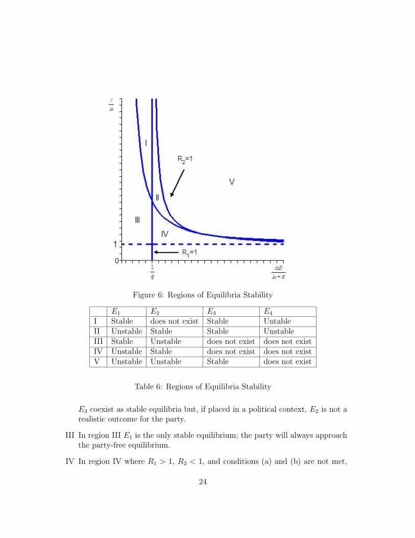
Figure 6: Regions of Equilibria Stability

E1 E2 E3 E4

I Stable does not exist Stable UntableII Unstable Stable Stable UnstableIII Stable Unstable does not exist does not existIV Unstable Stable does not exist does not existV Unstable Unstable Stable does not exist

Table 6: Regions of Equilibria Stability

E3 coexist as stable equilibria but, if placed in a political context, E2 is not arealistic outcome for the party.

III In region III E1 is the only stable equilibrium; the party will always approachthe party-free equilibrium.

IV In region IV where R1 > 1, R2 < 1, and conditions (a) and (b) are not met,

24

E2, the member-free state, is the only stable equilibrium.

V In region V where both R1 > 1 and R2 > 1 and conditions (a) and (b) are notmet, E3 is the only stable equilibrium; the party will inevitably approach anendemic state.

5 The Green Party of Pennsylvania: A Case Study

After discussing hypothetical parameters in backward bifurcation and sensitivityanalysis, we employ real world data from the Green Party to derive parameters andfurther analyze the model.

5.1 Parameter Estimation for the One-Track Model

In our discussion, we estimate the model’s parameters based on the data from theGreen Party of Pennsylvania. We use voter registration for the Green Party in placeof party membership to distinguish between V and M because we could not obtaindata concerning Green Party membership. We initially restricted our complex modelto party membership in order to incorporate the 22 states in which voters cannotregister to specific parties; however, in the case where access to membership data islimited we measure party registration. In other words, we replace membership withparty registration in this particular case study and, for purposes of consistency, werefer to registered voters as M individuals.

After contacting the national Green Party directly, we obtained (1) the numberof registered voters in the Green Party of Pennsylvania sampled over the years2001 to 2005 and (2) access to the number of votes received by all Green Partycandidates running in Pennsylvania since the state party’s founding. However, dueto the lack of data on the net votes cast for Green Party candidates we referenced aparticular campaign to obtain parameters dependent on the number of individualsin V . Due to limited data we also roughly approximated certain parameters (i.e.the augmentation factor α).

We justify our motivation in choosing the state of Pennsylvania because (1) thetotal population of Pennsylvania has increased only 1.01 % from 2000 to 2004, a lowenough increase that allows us to assume constant population, N , and consistency ofsocial structure (i.e., no resulting movement between H and L) [20] and (2) the dataoffered from Pennsylvania was free of drastic changes in M that might be associatedwith exceptional candidates or highly specific events. Our parameter estimationsfollow:

25

(1) µ = 0.014: µ, the exit rate from the system, is essentially the average deathrate of people in the voting age population. We calculate the parameter by di-viding 128,010, the number of deaths in the voting age population in 2002(ages18 and above since individuals become eligible to vote at 18), by 9,358,833,the number of individuals in the voting age population in 2002 [20]. We applya unit of time−1 to µ.

(2) γ = 115.16: We assign γ, the recruitment rate of V individuals into the regis-tered class, M , a numerical value by using the relationship ∆M

∆t= γ V M

Nwhere

∆M is the increase in M per unit time, MN

is the the proportion of M individ-uals in the N voting population and V is the total number of voters excludingregistered voters. We use the following data to calculate γ : (1)∆M

∆tis esti-

mated by the increase in Green Party registration over a specific time period(i.e., one year), (2) M

Nis derived by dividing the number of Green Party reg-

istered individuals by the total voting population N and (3) the total numberof Green Party voters, V , is measured by the votes received in a particularelection subtracted by the number of registered Green Party voters in the sameyear (we find the difference in order to isolate simply those who vote Greenbut are not registered for the party).

Even though we received data of the number of registered Green Party votersin the state of Pennsylvania from 2001 to 2005, we did not have access to thetotal number of Green Party voters excluding registered voters. We avoidedthis obstacle by referencing the gubernatorial campaign of Michael Morrill on11/05/2002 in Pennsylvania in which he received 38,030 votes (i.e., 1.1 % ofthe total votes) and, after subtracting the 3266 registered green party votersat the time [13], we arrive at a voting population V of 34,814 individuals.Note that we assume that all registered Green Party voters voted for Morrill,a relatively safe assumption given the higher level of commitment by registeredvoters to the party and the relative importance of a gubernatorial election.

In order to determine the proportion MN

we calculated N , the number of vot-ers in the voting age population in 2002, by multiplying 9,358,833, the totalnumber of individuals in the voting age population (ages 18 and up), by thevoter turnout for this particular election, 37.39 % (close to the average voterturnout of 38.4 % [21]). We combine these elements in the following quotient:γ = (∆M

∆T)( V

MN

). Substituting in the appropriate values, γ = 3742(0.00093)(34814)

.

After performing the calculation we find that γ = 115.16, an exceptionallyhigh value implying that the third party will soon become a majority party

26

via such a high initial recruitment rate of members, a rather improbable sit-uation. In other words, this value of γ bodes too well for the third party.However, the prediction of an outcome as unlikely as the rapid increase of thethird party to the ranks of a majority party provides support for the necessityof the two-track model, which assumes heterogeneous mixing of susceptibleswith different affinities to the third party ideology. Therefore, while γ maybe initially high due to the availability and high susceptibility of individualsin H, L susceptibles will be particularly resistant to the ideology, in effect,reducing the recruitment into V and thus into M . Over time, a depletion inthe H class due to the conversion of its individuals into the V class along withthe resistance from the L class will cause γ to decrease with time as the initialfervor of member and voter recruitment decreases. We apply a unit of time−1

to γ.

(3) α: We referenced literature regarding the methods and hourly commitmentof party members to voter recruitment and approximated that registered vot-ers are roughly three times as effective in recruiting Green Party voters asindividuals from V [10]. We do not apply units to α given that α is a scalar.

(4) τ : We do not consider τ for the one-track model since we assume homogeneityof the susceptible population (i.e., we do not have two classes with differentrecruitment rates from V to S). We do not apply units to τ given that τ is ascalar.

(5) ε: We regard ε as the linear term representing the role of secondary sources (i.e.,the media) in affecting a voter’s decision. In the case of the Democratic vote,studies show that during a period of low political information, the predictedprobability of a Democratic vote drops from about 0.65 to about 0.55 while athigh levels of information (i.e., just prior to elections), there is an independent,media-influenced movement from a 0.4 to 0.6 probability of voting Democratin 1994 [15]. Assuming that such a phenomenon can be observed in anyindividual who votes and assuming a medium information flow, we averagethe difference of the changes in probability during low and high informationflow and obtain 0.05 as the value for ε. We apply a unit of time−1 to ε.

It is very difficult to obtain politically realistic projections of the endemic state ifwe apply these data-derived parameters of which only µ does not incorporate somedegree of approximation. With such a high γ value, the one-track model bifurcationplot projects an immediate rise of the third party to majority status. Therefore,while it is useful to derive parameters from actual data, we avoid unrealistic projec-tions for the one-track model by considering the aforementioned ideal set of parame-

27

ters used in both the backward bifurcation and sensitivity analysis sections. Fromthese idealized parameters we offer advice as to how third parties can strategize andgrow by changing their recruitment efforts to match the ideal set of parameters.

6 The Two-Track Model

After thoroughly examining the one-track model, deriving conclusions and provid-ing recommendations, we perform analysis on the original, heterogenous two trackmodel. We begin by obtaining the party free equilibrium (PFE) and the first tip-ping point, R′

1, which is analogous to R1 in the one track model. We find thatdetermining any other equilibria or thresholds analytically is too complicated andwe cannot extract anything politically relevant from further analysis; therefore, welook at equilibria stability numerically by fixing parameter values in the Jacobianmatrices. We then present deterministic simulations to observe the outcomes of thevarious equilibrium conditions. Finally, we offer bifurcation diagrams for the modeland analyze the outcomes.

6.1 Analysis

6.1.1 The Party-Free Equilibrium (PFE) and the Threshold/TippingPoint R′

1

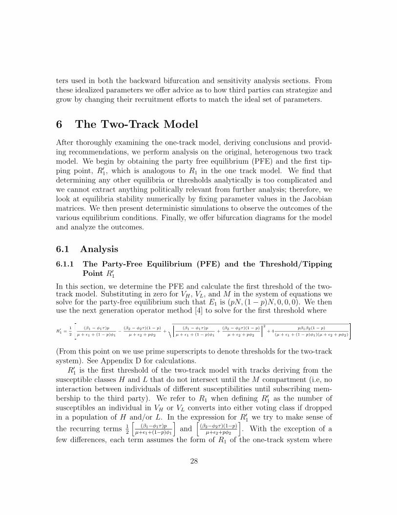
In this section, we determine the PFE and calculate the first threshold of the two-track model. Substituting in zero for VH , VL, and M in the system of equations wesolve for the party-free equilibrium such that E1 is (pN, (1− p)N, 0, 0, 0). We thenuse the next generation operator method [4] to solve for the first threshold where

R′1 =

1

2

264 (β1 − φ1τ)p

µ + ε1 + (1 − p)φ1−

(β2 − φ2τ)(1 − p)

µ + ε2 + pφ2+

vuut" (β1 − φ1τ)p

µ + ε1 + (1 − p)φ1+

(β2 − φ2τ)(1 − p)

µ + ε2 + pφ2

#2+ 4

pβ1β2(1 − p)

(µ + ε1 + (1 − p)φ1)(µ + ε2 + pφ2)

375

(From this point on we use prime superscripts to denote thresholds for the two-tracksystem). See Appendix D for calculations.

R′1 is the first threshold of the two-track model with tracks deriving from the

susceptible classes H and L that do not intersect until the M compartment (i.e, nointeraction between individuals of different susceptibilities until subscribing mem-bership to the third party). We refer to R1 when defining R′

1 as the number ofsusceptibles an individual in VH or VL converts into either voting class if droppedin a population of H and/or L. In the expression for R′

1 we try to make sense of

the recurring terms 12

[(β1−φ1τ)p

µ+ε1+(1−p)φ1

]and

[(β2−φ2τ)(1−p)

µ+ε2+pφ2

]. With the exception of a

few differences, each term assumes the form of R1 of the one-track system where

28

R1 = β−φµ+ε

; for that reason, we designate the first recurring term as R′H (concerned

with the dynamics of the H track) and the second term R′L (concerned with the

dynamics of the L track). We treat these tracks separately because R′1 is primarily

concerned with the susceptible transition to the third party voting stage at whichthe tracks remain independent (i.e., individuals from different tracks do not .

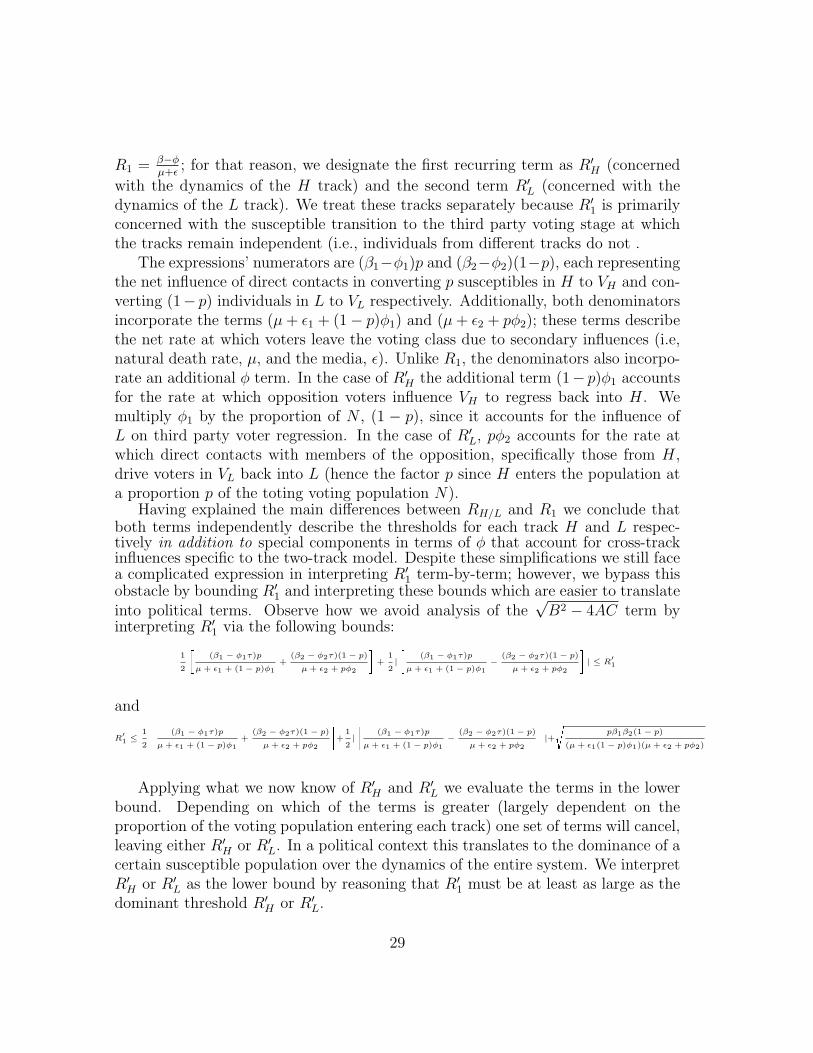
The expressions’ numerators are (β1−φ1)p and (β2−φ2)(1−p), each representingthe net influence of direct contacts in converting p susceptibles in H to VH and con-verting (1− p) individuals in L to VL respectively. Additionally, both denominatorsincorporate the terms (µ + ε1 + (1− p)φ1) and (µ + ε2 + pφ2); these terms describethe net rate at which voters leave the voting class due to secondary influences (i.e,natural death rate, µ, and the media, ε). Unlike R1, the denominators also incorpo-rate an additional φ term. In the case of R′

H the additional term (1− p)φ1 accountsfor the rate at which opposition voters influence VH to regress back into H. Wemultiply φ1 by the proportion of N , (1 − p), since it accounts for the influence ofL on third party voter regression. In the case of R′

L, pφ2 accounts for the rate atwhich direct contacts with members of the opposition, specifically those from H,drive voters in VL back into L (hence the factor p since H enters the population ata proportion p of the toting voting population N).

Having explained the main differences between RH/L and R1 we conclude thatboth terms independently describe the thresholds for each track H and L respec-tively in addition to special components in terms of φ that account for cross-trackinfluences specific to the two-track model. Despite these simplifications we still facea complicated expression in interpreting R′

1 term-by-term; however, we bypass thisobstacle by bounding R′

1 and interpreting these bounds which are easier to translateinto political terms. Observe how we avoid analysis of the

√B2 − 4AC term by

interpreting R′1 via the following bounds:

1

2

"(β1 − φ1τ)p

µ + ε1 + (1 − p)φ1+

(β2 − φ2τ)(1 − p)

µ + ε2 + pφ2

#+

1

2|"

(β1 − φ1τ)p

µ + ε1 + (1 − p)φ1−

(β2 − φ2τ)(1 − p)

µ + ε2 + pφ2

#| ≤ R

′1

and

R′1 ≤

1

2

"(β1 − φ1τ)p

µ + ε1 + (1 − p)φ1+

(β2 − φ2τ)(1 − p)

µ + ε2 + pφ2

#+

1

2|"

(β1 − φ1τ)p

µ + ε1 + (1 − p)φ1−

(β2 − φ2τ)(1 − p)

µ + ε2 + pφ2

#|+

spβ1β2(1 − p)

(µ + ε1(1 − p)φ1)(µ + ε2 + pφ2)

Applying what we now know of R′H and R′

L we evaluate the terms in the lowerbound. Depending on which of the terms is greater (largely dependent on theproportion of the voting population entering each track) one set of terms will cancel,leaving either R′

H or R′L. In a political context this translates to the dominance of a

certain susceptible population over the dynamics of the entire system. We interpretR′

H or R′L as the lower bound by reasoning that R′

1 must be at least as large as thedominant threshold R′

H or R′L.

29

The upper bound considers both (1) the dominant threshold term of the lower

bound and (2) an additional expression√

pβ1β2(1−p)(µ+ε1(1−p)φ1)(µ+ε2+pφ2)

. Similar to the ad-

ditional φ terms in the denominator of the R′H and R′

L, (2) is a cross-track termthat accounts for interaction between the two tracks. Analytically, it translates tothe geometric mean of both thresholds that, when added to the dominant threshold,constitutes the upper bound of R′

1.In order for the PFE to be unstable we need R′

1 > 1. In other words, using thethreshold definition from the one-track model, if an individual from either VH , VL

or M is introduced in a population of H and L, he/she must convert more thanone susceptible into third party voters in order to establish the V class. Similar tothe one-track model, a sufficient initial number of members can bypass stability ofthe PFE as can be observed in the backward bifurcation section for the two-trackmodel. (See section 5.3). Due to the parallels between the one and two-track R1

and R′1 thresholds most recommendations on voter recruitment made earlier in the

sensitivity analysis section of the one-track model pertain to the two-track model.

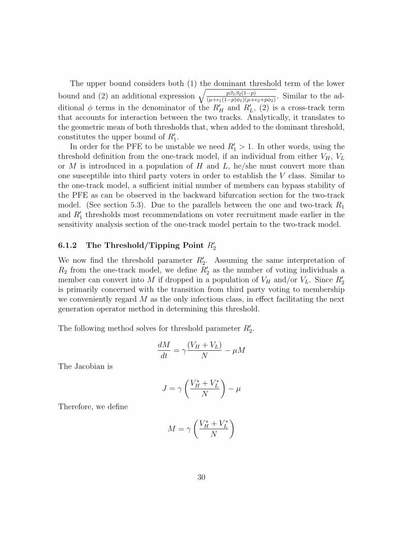
6.1.2 The Threshold/Tipping Point R′2

We now find the threshold parameter R′2. Assuming the same interpretation of

R2 from the one-track model, we define R′2 as the number of voting individuals a

member can convert into M if dropped in a population of VH and/or VL. Since R′2

is primarily concerned with the transition from third party voting to membershipwe conveniently regard M as the only infectious class, in effect facilitating the nextgeneration operator method in determining this threshold.

The following method solves for threshold parameter R′2.

dM

dt= γ

(VH + VL)

N− µM

The Jacobian is

J = γ

(V ∗

H + V ∗L

N

)− µ

Therefore, we define

M = γ

(V ∗

H + V ∗L

N

)

30

and

D = µ

MD−1 =γ

µ

(V ∗

H + V ∗L

N

)Since the matrix only has one eigenvalue we conclude that

R′2 = MD−1 =

γ

µ

(V ∗

H + V ∗L

N

)Note the similarity of R′

2 to R2 of the one-track model from which we expectedsomething of the form γ

µ(1− 1

R1). While R′

2 is not expressed explicitly, given the useof the terms V ∗

H and V ∗L , we can still make conclusions about the two-track model

numerically.

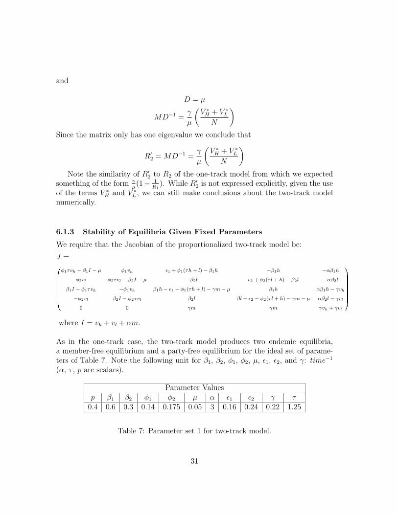
6.1.3 Stability of Equilibria Given Fixed Parameters

We require that the Jacobian of the proportionalized two-track model be:

J =0BBBBBBBB@

φ1τvh − β1I − µ φ1vh ε1 + φ1(τh + l)− β1h −β1h −αβ1h

φ2vl φ2τvl − β2I − µ −β2l ε2 + φ2(τl + h)− β2l −αβ2l

β1I − φ1τvh −φ1vh β1h− ε1 − φ1(τh + l)− γm− µ β1h αβ1h− γvh

−φ2vl β2I − φ2τvl β2l βl − ε2 − φ2(τl + h)− γm− µ αβ2l − γvl

0 0 γm γm γvh + γvl

1CCCCCCCCA

where I = vh + vl + αm.

As in the one-track case, the two-track model produces two endemic equilibria,a member-free equilibrium and a party-free equilibrium for the ideal set of parame-ters of Table 7. Note the following unit for β1, β2, φ1, φ2, µ, ε1, ε2, and γ: time−1

(α, τ , p are scalars).

Parameter Valuesp β1 β2 φ1 φ2 µ α ε1 ε2 γ τ

0.4 0.6 0.3 0.14 0.175 0.05 3 0.16 0.24 0.22 1.25

Table 7: Parameter set 1 for two-track model.

31

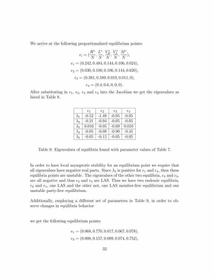
We arrive at the following proportionalized equilibrium points:

ei = (H∗

N,L∗

N,V ∗

H

N,V ∗

L

N,M∗

N),

e1 = (0.242, 0.484, 0.144, 0.106, 0.024),

e2 = (0.030, 0.100, 0.106, 0.144, 0.620),

e3 = (0.381, 0.589, 0.019, 0.011, 0),

e4 = (0.4, 0.6, 0, 0, 0).

After substituting in e1, e2, e3 and e4 into the Jacobian we get the eigenvalues aslisted in Table 8.

e1 e2 e3 e4

λ1 -0.52 -1.48 -0.05 -0.05λ2 -0.21 -0.94 -0.05 -0.05λ3 0.016 -0.05 -0.69 0.010λ4 -0.05 -0.08 -0.90 -0.45λ5 -0.05 -0.15 -0.05 -0.05

Table 8: Eigenvalues of equilibria found with parameter values of Table 7.

In order to have local asymptotic stability for an equilibrium point we require thatall eigenvalues have negative real parts. Since λ3 is positive for e1 and e4, then theseequilibria points are unstable. The eigenvalues of the other two equilibria, e2 and e3,are all negative and thus e2 and e3 are LAS. Thus we have two endemic equilibria,e2 and e1, one LAS and the other not, one LAS member-free equilibrium and oneunstable party-free equilibrium.

Additionally, employing a different set of parameters in Table 9, in order to ob-serve changes in equilibria behavior

we get the following equilibrium points:

e1 = (0.068, 0.770, 0.017, 0.067, 0.078),

e2 = (0.008, 0.157, 0.009, 0.074, 0.752),

32

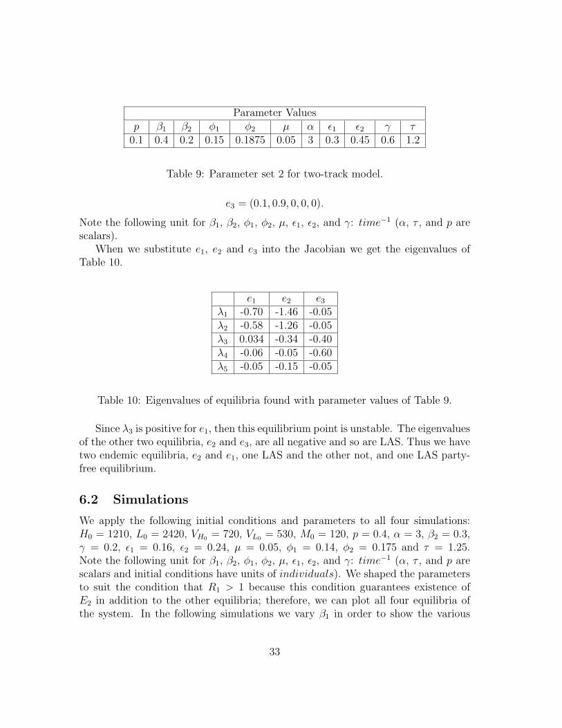
Parameter Valuesp β1 β2 φ1 φ2 µ α ε1 ε2 γ τ

0.1 0.4 0.2 0.15 0.1875 0.05 3 0.3 0.45 0.6 1.2

Table 9: Parameter set 2 for two-track model.

e3 = (0.1, 0.9, 0, 0, 0).

Note the following unit for β1, β2, φ1, φ2, µ, ε1, ε2, and γ: time−1 (α, τ , and p arescalars).

When we substitute e1, e2 and e3 into the Jacobian we get the eigenvalues ofTable 10.

e1 e2 e3

λ1 -0.70 -1.46 -0.05λ2 -0.58 -1.26 -0.05λ3 0.034 -0.34 -0.40λ4 -0.06 -0.05 -0.60λ5 -0.05 -0.15 -0.05

Table 10: Eigenvalues of equilibria found with parameter values of Table 9.

Since λ3 is positive for e1, then this equilibrium point is unstable. The eigenvaluesof the other two equilibria, e2 and e3, are all negative and so are LAS. Thus we havetwo endemic equilibria, e2 and e1, one LAS and the other not, and one LAS party-free equilibrium.

6.2 Simulations

We apply the following initial conditions and parameters to all four simulations:H0 = 1210, L0 = 2420, VH0 = 720, VL0 = 530, M0 = 120, p = 0.4, α = 3, β2 = 0.3,γ = 0.2, ε1 = 0.16, ε2 = 0.24, µ = 0.05, φ1 = 0.14, φ2 = 0.175 and τ = 1.25.Note the following unit for β1, β2, φ1, φ2, µ, ε1, ε2, and γ: time−1 (α, τ , and p arescalars and initial conditions have units of individuals). We shaped the parametersto suit the condition that R1 > 1 because this condition guarantees existence ofE2 in addition to the other equilibria; therefore, we can plot all four equilibria ofthe system. In the following simulations we vary β1 in order to show the various

33

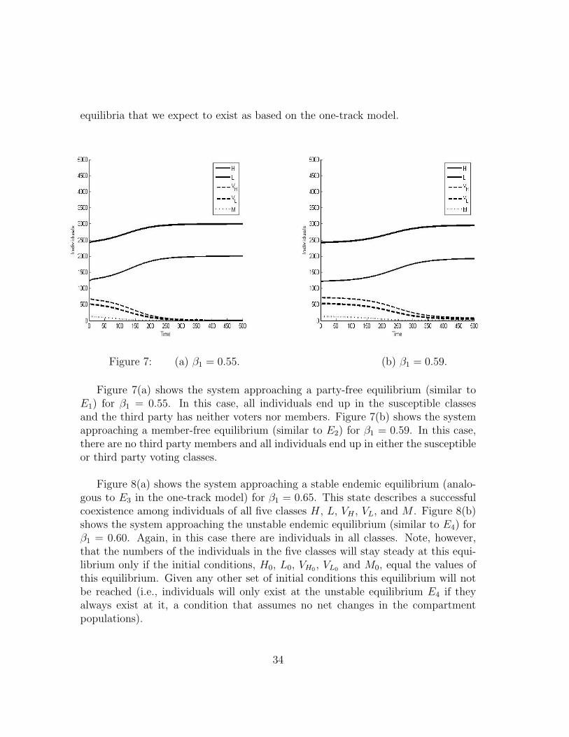
equilibria that we expect to exist as based on the one-track model.

Figure 7: (a) β1 = 0.55. (b) β1 = 0.59.

Figure 7(a) shows the system approaching a party-free equilibrium (similar toE1) for β1 = 0.55. In this case, all individuals end up in the susceptible classesand the third party has neither voters nor members. Figure 7(b) shows the systemapproaching a member-free equilibrium (similar to E2) for β1 = 0.59. In this case,there are no third party members and all individuals end up in either the susceptibleor third party voting classes.

Figure 8(a) shows the system approaching a stable endemic equilibrium (analo-gous to E3 in the one-track model) for β1 = 0.65. This state describes a successfulcoexistence among individuals of all five classes H, L, VH , VL, and M . Figure 8(b)shows the system approaching the unstable endemic equilibrium (similar to E4) forβ1 = 0.60. Again, in this case there are individuals in all classes. Note, however,that the numbers of the individuals in the five classes will stay steady at this equi-librium only if the initial conditions, H0, L0, VH0 , VL0 and M0, equal the values ofthis equilibrium. Given any other set of initial conditions this equilibrium will notbe reached (i.e., individuals will only exist at the unstable equilibrium E4 if theyalways exist at it, a condition that assumes no net changes in the compartmentpopulations).

34

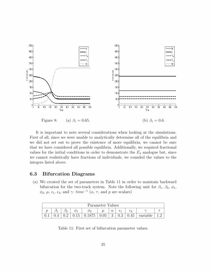
Figure 8: (a) β1 = 0.65. (b) β1 = 0.6.

It is important to note several considerations when looking at the simulations.First of all, since we were unable to analytically determine all of the equilibria andwe did not set out to prove the existence of more equilibria, we cannot be surethat we have considered all possible equilibria. Additionally, we required fractionalvalues for the initial conditions in order to demonstrate the E4 analogue but, sincewe cannot realistically have fractions of individuals, we rounded the values to theintegers listed above.

6.3 Bifurcation Diagrams

(a) We created the set of parameters in Table 11 in order to maintain backwardbifurcation for the two-track system. Note the following unit for β1, β2, φ1,φ2, µ, ε1, ε2, and γ: time−1 (α, τ , and p are scalars)

Parameter Valuesp β1 β2 φ1 φ2 µ α ε1 ε2 γ τ

0.1 0.4 0.2 0.15 0.1875 0.05 3 0.3 0.45 variable 1.2

Table 11: First set of bifurcation parameter values.

35

In order to create the above parameter set we varied β, ε, and φ, approxi-mating the degree by which the corresponding parameters varied. We usedintuition in order to approximate the relative factor by which, for example,β1 exceeds β2. As it turns out, our approximations of the relative differencesbetween corresponding parameters still maintained backward bifurcation.

We started off by assuming that the portion of the population entering theH class, p, was 0.1. This decision was motivated by (1) the considerationthat the Green Party, given its highly progressive, typically youth-cateringagenda directly appeals to about 10 percent of the total voting population(i.e, individuals in a young, educated, progressive social sphere) and (2) theparameter value 0.1 gives us a more reasonable endemic equilibrium that doesnot approach majority status (approximately 1) as quickly as larger values forp. In determining relative β parameters we assumed that H susceptibles aretwice as likely to become voters as L susceptibles; this lower relative value isappropriate given that our methodology of placing individuals into H and Lvia the number of low versus high affinity factors of the individual lessens themagnitude of difference between the susceptible classes. For ε we assumed thatopposition media and other secondary influences would factor 1.5 times morein VL regression back to L than in the transition of VH back to H. Likewise, φ2

is 1.25 times greater than φ1 because, as with ε, φ is greater for L susceptibleswho are more resistant to third party ideology.

Figure 9, the bifurcation diagram for this parameter set, shows the possiblebehaviors of the member class M by varying γ. We observe that the minimumvalue of γ that would give hope to the party is 0.28 because neither endemicequilibrium exists for γ < 0.28. However, given γ > 0.28 and a certain initialnumber of members M , the party can approach a stable endemic equilibrium.We observe the general trend that the larger our value of γ the larger the valuesof the endemic equilibrium. An important conclusion we make concerningthe parallels between the one-track and two-track models is how, even whenR1 < 1, the party can thrive in both tracks given that γ is large enough.

(b) A second set of parameters in Table 12 considers the case when p = 0.05, acondition in which the third party targets a high affinity class that comprisesonly 5 percent of the total voting population:

We start off by assuming that the portion of the population entering the Hclass, p, is 0.05, a situation pertaining to third parties with highly specific,

36

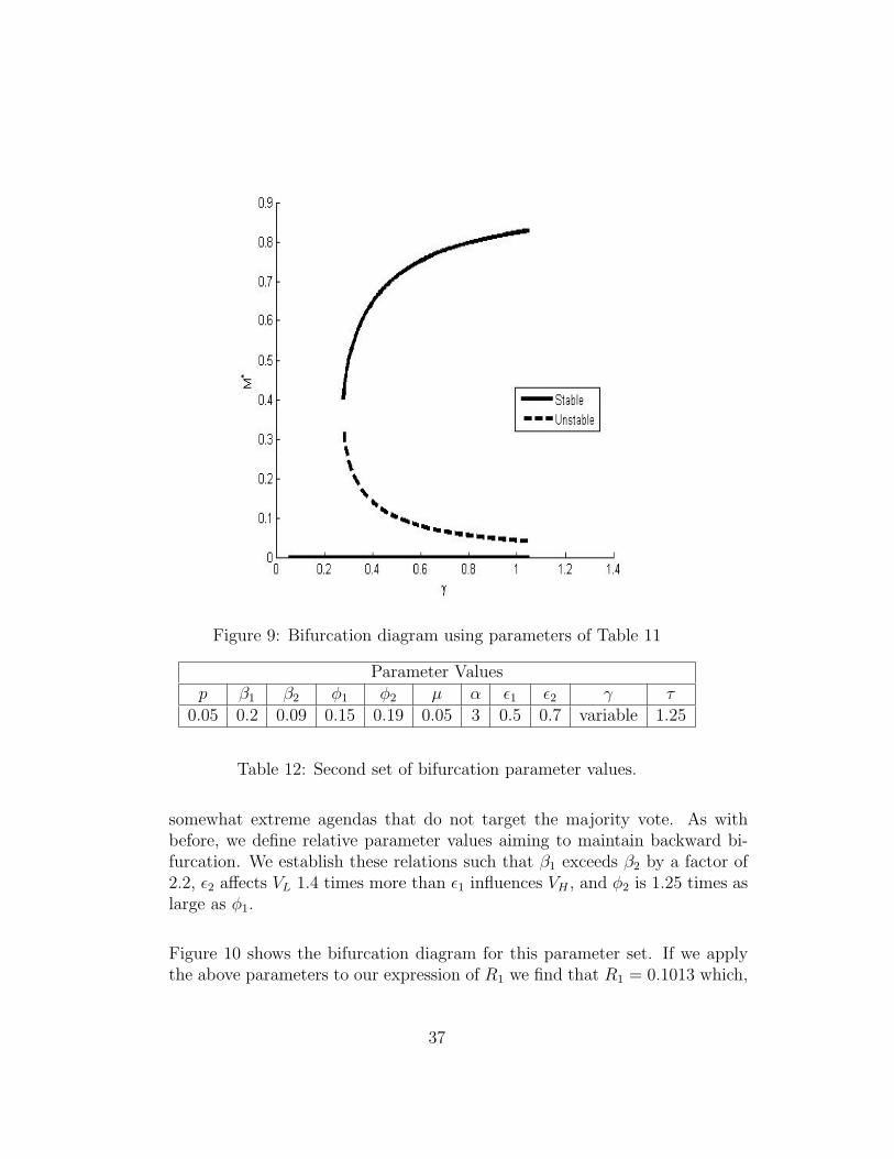
Figure 9: Bifurcation diagram using parameters of Table 11

Parameter Valuesp β1 β2 φ1 φ2 µ α ε1 ε2 γ τ

0.05 0.2 0.09 0.15 0.19 0.05 3 0.5 0.7 variable 1.25

Table 12: Second set of bifurcation parameter values.

somewhat extreme agendas that do not target the majority vote. As withbefore, we define relative parameter values aiming to maintain backward bi-furcation. We establish these relations such that β1 exceeds β2 by a factor of2.2, ε2 affects VL 1.4 times more than ε1 influences VH , and φ2 is 1.25 times aslarge as φ1.

Figure 10 shows the bifurcation diagram for this parameter set. If we applythe above parameters to our expression of R1 we find that R1 = 0.1013 which,

37

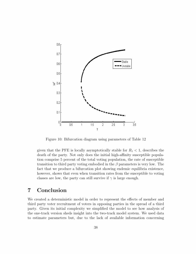
Figure 10: Bifurcation diagram using parameters of Table 12

given that the PFE is locally asymptotically stable for R1 < 1, describes thedeath of the party. Not only does the initial high-affinity susceptible popula-tion comprise 5 percent of the total voting population, the rate of susceptibletransition to third party voting embodied in the β parameters is very low. Thefact that we produce a bifurcation plot showing endemic equilibria existence,however, shows that even when transition rates from the susceptible to votingclasses are low, the party can still survive if γ is large enough.

7 Conclusion

We created a deterministic model in order to represent the effects of member andthird party voter recruitment of voters in opposing parties in the spread of a thirdparty. Given its initial complexity we simplified the model to see how analysis ofthe one-track version sheds insight into the two-track model system. We used datato estimate parameters but, due to the lack of available information concerning

38

net votes cast for Green Party candidates, our estimated parameters provided littlevaluable information. Therefore, instead we created ideal sets of parameters forboth the one and two-track systems in order to obtain a state of class coexistenceand translated these ideal parameters into political terms via strategies that partiescan take to initiate growth. Many of our recommendations derive from consideringseveral scenarios the party might take in terms of the thresholds or tipping points R1,R2, and R′

1 (analogous to R1 of the simple model). We regard these tipping points asdecisive factors in the behavior of the party since they explain how voter recruitmentand opposition efforts, embodied in the values of the system’s parameters, can drivea voting population to death, growth, or unstable stagnancy (i.e., the steady stateE3) depending on the parameters used. Hence, we translate parameters of relativemagnitude into strategies that politicians can use in spreading a third party.

For example, consider a voting population N . Mathematically speaking, thepopulation can assume four different outcomes: the party dies out, members die outbut opposition voters and party voters remain, and all classes coexist in either anunstable or stable state. In the political context, however, we only consider two ofthe possible outcomes since (1) a member-free equilibrium implies that voters votefor a party that does not exist (where we assume that parties require members forexistence) and (2) the population cannot tend to and stay at the unstable endemicequilibrium unless the number of individuals in each compartment stays fixed (ahighly unlikely scenario given the local dynamics of the system where individualstravel between classes).

We now have two possible outcomes: party death or party growth. For the firstoption, the party dies out if R1 < 1 and the population will always tend to thisstate given that the net flow into V , measured as β − φ is less than oppositionfrom the media and the natural exit rate of voters from the system embodied inµ + ε. Therefore, the party dies out unless a stable endemic equilibrium also existsthat guarantees a stable state of class coexistence at which susceptibles, voters, andmembers exist (i.e., the party grows because it has voters and members needed torecruit susceptibles). Backward bifurcation plots of both the one and two-track sys-tems demonstrate the coexistence of the PFE and endemic equilibrium. Therefore,the party can assume two tracks: death or growth where the deciding factor is theinitial number of members in the system that, if large enough, can overcome theparty’s tendency to death.

The case where R1 > 1 and R2 < 1 is similar to the previous case except thatthere is an additional stable member-free equilibrium. However, as we stated earlier,we will not be considering this scenario in a political context.

On the other hand, if R2 > 1, then only the endemic equilibrium will be stable.Then, so long as there is at least one member, the result will be coexistence of all

39

classes. However, this does not seem likely since all bifurcation diagrams that showthis case would imply that a majority of the voting population would become thirdparty members. Given that we study a third party, this outcome seems unrealistic.

In addition to running deterministic simulations of both systems that show thetendency of the population to all four equilibria states, we performed sensitivityanalysis to determine those parameters to which our system was most sensitive.Not surprisingly, β, the recruitment rate of susceptibles into the voting class byvoters and members (with the augmentation factor α), emerged as the most sensi-tive parameter, followed by φ and γ. This indicates that the S-to-V transition ismost important initially since it builds up the population of V . Only after V hasaccumulated a substantial number of individuals should the party focus on the Vto M transition by accruing members with an effort γ. Then, once more membershave joined, the party grows even faster since members recruit opposition voters atan increased factor α.

Even though we used available data to estimate parameters, we ultimately usedideal parameters to model the desired state of endemic coexistence among all classes.Our model does not aim to predict the future of third parties, but rather to offerrecruitment strategies to parties so that they might grow and spread within a votingpopulation. We conclude with the final advice that parties should build up thenumber of initial members in the party since, if R1 < 1, this value ultimatelydetermines the fate of the party: death or growth.

8 Acknowledgements

We would like to thank our principal advisors Christopher Kribs-Zaleta, Karen Rıos-Soto, and Carlos Castillo-Chavez. Additionally, we thank Linda Gao, Baojun Song,Armando Arciniega, Leon Arriola, and all other MTBI participants and LANL af-filiates for their help and advice.

This research has been partially supported by grants from the National SecurityAgency, the National Science Foundation, the T Division of Los Alamos NationalLab (LANL), the Sloan Foundation, and the Office of the Provost of Arizona StateUniversity. The authors are solely responsible for the views and opinions expressedin this research; it does not necessarily reflect the ideas and/or opinions of thefunding agencies, Arizona State University, or LANL.

40

References

[1] Arriola, L. and J. Hyman, Summer 2005. Forward and Adjoint SensitivityAnalysis: With Applications in Dynamical Systems, Linear Algebra and Opti-mization. 3.

[2] Bass, L., and L. Casper, 2001. Impacting the political landscape: who registersand votes among naturalized Americans? Political Behavior,23(2),103-130.

[3] Bettencourt, L., Cintron-Arias, A., Kaiser, D., and C. Castillo-Chavez, 2005.The power of a good idea: quantitative modeling of the spread of ideas fromepidemiological models. Not printed,LAUR-05-0485, MIT-CTP-3589.

[4] Brauer, F., and C. Castillo-Chavez. Mathematical Models in Population Biologyand Epidemiology Springer-Verlag, NY 2001.

[5] Burbank, M., 1997. Explaining contextual effects on vote choice. PoliticalBehavior,19(2),113-132.

[6] Castillo-Chavez, C., and B. Song, 2003. Models for the Transmission Dynam-ics of Fanatic Behaviors. Bioterrorism: Mathematical Modeling Applications inHomeland Security (SIAM Frontier Series in Applied Mathematics). 155-172.H. T. Banks and Carlos Castillo-Chavez, eds. SIAM, Philadelphia, PA.

[7] Castillo-Garsow, M., Henson, L., Mejran, L., Rıos-Soto, K.R., and B. Song.Raves, clubs, and ecstasy: The impact of peer pressure. Cornell Univ., Dept.of Biometrics Technical Report,BU-1581-M.

[8] Crisosto, N., Castillo-Chavez, C., Kribs-Zaleta, C., and S. Wirkus, 2002. Com-munity Resilience in Collaborative Learning. Submitted to Journal of the Learn-ing Sciences, September 2002.

[9] Franklin and Marshall. General Election Turnout for Governor, Jul. 25, 2005,http://www.fandm.edu/x4527.xml.

[10] Gerber, A., and D. Green, 2000. The effects of canvassing, telephone calls, anddirect mail on voter turnout: a field experiment. American Political ScienceReview,94(3),653-663.

[11] Gladwell, Malcolm. The Tipping Point. The New Yorker, June 1996.

[12] Gonzalez, B., Huerta-Sanchez, E., Kribs-Zaleta, C., Ortiz-Nieves, A., and T.Vazquez-Alvarez. Am I Too Fat?: Bulimia as an Epidemic. Cornell Univ., Dept.of Biometrics Technical Report,BU-1578-M.

41

[13] Green Party Ballot Status and Voter Registration Totals. July 22, 2005,http://web.greens.org/stats/.

[14] Green Party of the United States. Ten Key Values of the Green Party. July 14,2005. http://gp.org/tenkey.shtml.

[15] Jackman, S. 2003. Moderating the News: Political Information, Media Effectsand the role of Political Institutions. Unpublished manuscript, Department ofPolitical Science, Stanford University, Stanford, CA.

[16] Kowalewski, D., 1995. How movements move: the dynamics of an ecoprotestcampaign. The Social Science Journal,32(1),49-67.

[17] Southwell, P.L., 2003. The politics of alienation: nonvoting and sup-port of third-party candidates among 18-30-year-olds. The Social ScienceJournal,40(1),99-107.

[18] Southwell, P.L., 2004. Nader voters in the 2000 Presidential Election: whatwould they have done without him? The Social Science Journal,41(3),423-431.

[19] Timpone, R.J., 1998. Ties that bind: measurement, demographics, and socialconnectedness. Political Behavior,20(1),53-77.

[20] US Census Bureau. July 20, 2005, http://factfinder.census.gov/.

[21] Wial, H., 1999. Democracy in Pennsylvania.Keystone Research Center, 1-21.

[22] Wikipedia, the free encyclopedia. third party (United States). July 11, 2005.http://en.wikipedia.org/wiki/Third party (United States).

[23] Wong, J., 2000. The effects of age and political exposure on the developmentof party identification among Asian American and Latino immigrants in theUnited States. Political Behavior,22(4),341-371.

42

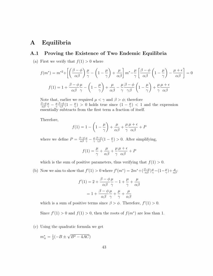
A Equilibria

A.1 Proving the Existence of Two Endemic Equilibria

(a) First we verify that f(1) > 0 where

f(m∗) = m∗2+

[(β − φ

αβ

)µ

γ−(

1− µ

γ

)+

µ

αβ

]m∗−µ

γ

[β − φ

αβ

(1− µ

γ

)− µ + ε

αβ

]= 0

f(1) = 1 +β − φ

αβ

µ

γ−(

1− µ

γ

)+

µ

αβ− µ

γ

β − φ

γβ

(1− µ

γ

)+

µ

γ

µ + ε

αβ

Note that, earlier we required µ < γ and β > φ; thereforeβ−φαβ

µγ− µ

γβ−φγβ

(1 − µγ) > 0 holds true since (1 − µ

γ) < 1 and the expression

essentially subtracts from the first term a fraction of itself.

Therefore,

f(1) = 1−(

1− µ

γ

)+

µ

αβ+

µ

γ

µ + ε

αβ+ P

where we define P = β−φαβ

µγ− µ

γβ−φγβ

(1− µγ) > 0. After simplifying,

f(1) =µ

γ+

µ

αβ+

µ

γ

µ + ε

αβ+ P

which is the sum of positive parameters, thus verifying that f(1) > 0.

(b) Now we aim to show that f ′(1) > 0 where f ′(m∗) = 2m∗+(β−φαβ

)µγ−(1− µ

γ)+ µ

αβ:

f ′(1) = 2 +β − φ

αβ

µ

γ− 1 +

µ

γ+

µ

αβ

= 1 +β − φ

αβ

µ

γ+

µ

γ+

µ

αβ

which is a sum of positive terms since β > φ. Therefore, f ′(1) > 0.

Since f ′(1) > 0 and f(1) > 0, then the roots of f(m∗) are less than 1.

(c) Using the quadratic formula we get

m∗± = 1

2(−B ±

√B2 − 4AC)

43

whereA = 1

B =

(β − φ

αβ

)µ

γ−(

1− µ

γ

)+

µ

αβ

C = −µ

γ

[β − φ

αβ

(1− µ

γ

)− µ + ε

αβ

]Assuming B < 0 then the vertex, −B

2, of f(m∗) is positive and, assuming

that B2 − 4AC > 0 so that f(m∗) has two real solutions, we infer that atleast one solution of f(m∗) is positive. We continue noting that since C > 0then f(0) > 0 and therefore both solutions are positive. Given two positivesolutions that are less than 1 we then claim that both solutions are in (0, 1);hence the existence of two positive endemic equilibria under the conditions:B < 0, C > 0 and B2−4AC > 0. Now that we have shown that B < 0, C > 0and B2− 4AC > 0 support the existence of two positive solutions, we need tofind under what conditions those statements are true.

(d) B < 0, C > 0 and B2 − 4AC > 0 will be true under the following conditions:

C > 0

if and only if

−µ

γ

[β − φ

αβ

(1− µ

γ

)− µ + ε

αβ

]> 0

(β − φ)

(1− µ

γ

)< (µ + ε)

β − φ

µ + ε

(1− µ

γ

)< 1

1− µ

γ<

µ + ε

β − φ

1− µ + ε

β − φ<

µ

γ

R2 =γ

µ

(1− µ + ε

β − φ

)< 1

We then impose B < 0 as an additional condition for the existence of endemicequilibria.

B < 0

44

if and only if1

αβ+

(β − φ

αβ+ 1

)1

γ<

1

µ

which, again, translates to B < 0 where B is defined on the previous page.

We require that B2 − 4AC ≥ 0 for the existence of m∗ (in order to avoidcomplex values of m∗

±). Substituting in the values of A, B and C we get:[µ

αβ+

(β − φ

αβ

)µ

γ− 1

]2

− 4µ

γ

[µ + ε

αβ− β − φ

αβ

(1− µ

γ

)]≥ 0

Expansion and summing like terms yields(µ

αβ

)2

+

(µ

γ

)2

− 2

(µ

γ

)2β − φ

αβ+

(µ

γ

)2(β − φ

αβ

)2

+ 1−

2µ

αβ

µ

γ+ 2

µ

αβ

µ

γ

β − φ

αβ− 2

µ

αβ− 2

µ

γ+ 2

µ

γ

β − φ

αβ− 4

µ

γ

ε

αβ≥ 0

Then by completing the square we get the following equations[µ

αβ−(

1− β − φ

αβ

)µ

γ+ 1

]2

≥ 4µ

αβ

(1 +

ε

γ

)Next we take the square root of both sides,∣∣∣∣ µ

αβ−(

1− β − φ

αβ

)µ

γ+ 1

∣∣∣∣ ≥ 2

õ

αβ

(1 +

ε

γ

)Since we require µ < γ and β > φ, then

µ

αβ−(

1− β − φ

αβ

)µ

γ+ 1 =

µ

αβ+

β − φ

αβ

µ

γ+

(1− µ

γ

)> 0

and so ∣∣∣∣ µ

αβ−(

1− β − φ

αβ

)µ

γ+ 1

∣∣∣∣ =µ

αβ−(

1− β − φ

αβ

)µ

γ+ 1

Then replacing the absolute value terms and rearranging we get

µ

γ≤ µ

αβ+

β − φ

αβ

µ

γ− 2

õ

αβ

(1 +

ε

γ

)+ 1

45

A.2 Determining the Stability of E3 and E4

LetA′ = 1

B′ =

[−(β − φ)

(1− 2µ

γ−m∗

)+ αβm + µ + ε + γm∗

]C ′ = −γm∗

[αβ

(1− µ

γ− 2m∗

)− (β − φ)µ

γ− µ

]The solutions of the characteristic equation are the eigenvalues of J(µ

γ, m∗

±), andthe stability of the endemic equilibria depend of the signs of their real parts. If thereal parts of both eigenvalues are negative then the we conclude that the endemicequilibrium is locally asymptotically stable.

The eigenvalues are given by

λ± =1

2(−B′ ±

√B′2 − 4C ′)

We note that if B′2−4C ′ < 0, then the endemic equilibrium is locally asymptoticallystable if B′ > 0. On the other hand, if B′2 − 4C ′ ≥ 0 then the endemic equilibriumis locally asymptotically stable if B′ > 0 and C ′ > 0.

We now prove that B′ > 0 always holds given m∗± > 0 (i.e., given m∗

± exists).

B′ > 0 holds when[−(β − φ)

(1− 2µ

γ−m∗

±

)+ αβm∗

± + µ + ε + γm∗±

]> 0

m∗±((β − φ) + αβ + γ) > (β − φ)− 2

µ

γ(β − φ)− (µ + ε)

m∗± >

(β − φ)− 2µγ(β − φ)− (µ + ε)

(β − φ) + αβ + γ

m∗± >

β−φαβ− 2µ

γβ−φαβ− µ+ε

αβ

β−φαβ

+ 1 + γαβ

=− γ

µC − µ(β−φ)

γαβ

β−φαβ

+ 1 + γαβ

Recall that C = −µγ[β−φ

αβ(1− µ

γ)− µ+ε

αβ].

46

Note that C > 0 (for the condition that R2 < 1), β > φ, and m∗± > 0 (refer to

the Appendix A.1, where we show that m∗± is contained in (0,1)). Therefore,

− γµC − µ(β−φ)

γαβ

β−φαβ

+ 1 + γαβ

< 0

and so B′ > 0 whenever m∗ is greater than a negative expression. Since this alwaysholds, then B′ > 0 is always true.

We now verify the C ′ > 0 criterion for local asymptotic stability of the endemicequilibria where R2 < 1 whenever m∗ > −B

2.

Recall that B = (β−φαβ

)µγ− (1− µ

γ) + µ

αβ.

C ′ > 0 on condition that

−γm∗[αβ

(1− µ

γ− 2m

)− (β − φ)µ

γ− µ

]> 0

−αβ +µ

γγβ + 2mαβ + (β − φ)

µ

γ+ µ > 0

m∗ >αβ(1− µ

γ

)− (β − φ)µ

γ− µ

2αβ

m∗ >1

2

(1− µ

γ− µ(β − φ)

γαβ− µ

αβ

)= −B

2

Therefore C ′ > 0 whenever m∗ > −B2.

We now try to tie together our findings to distinguish the two endemic equilib-ria. Having shown that B′ > 0 and C ′ > 0 where R2 < 1, we establish the necessarycriteria for LAS for E3 and E4 where m∗ > −B

2

Recalling thatm∗± =

1

2

24− ��β − φ

αβ

�µ

γ−�

1−µ

γ

�+

µ

αβ

�±

s��−

β − φ

αβ

�µ

γ+

�1−

µ

γ

�−

µ

αβ

�2+ 4

�µ

γ

��β − φ

αβ

�1−

µ

γ

�−

µ + ε

αβ

�35

=1

2(−B ±

√B2 − 4C)

Since m∗+ > −B

2, E3 is LAS.

And since m∗− < −B

2, then E4 is unstable.

47

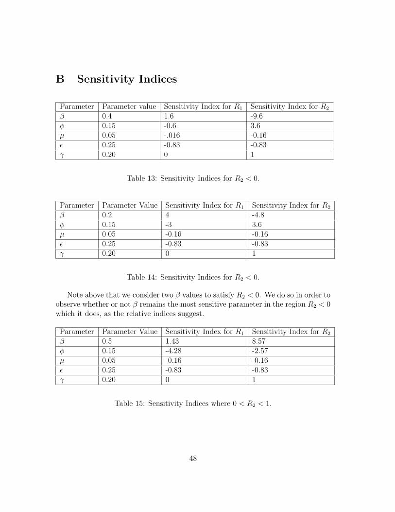
B Sensitivity Indices

Parameter Parameter value Sensitivity Index for R1 Sensitivity Index for R2

β 0.4 1.6 -9.6φ 0.15 -0.6 3.6µ 0.05 -.016 -0.16ε 0.25 -0.83 -0.83γ 0.20 0 1

Table 13: Sensitivity Indices for R2 < 0.

Parameter Parameter Value Sensitivity Index for R1 Sensitivity Index for R2

β 0.2 4 -4.8φ 0.15 -3 3.6µ 0.05 -0.16 -0.16ε 0.25 -0.83 -0.83γ 0.20 0 1

Table 14: Sensitivity Indices for R2 < 0.

Note above that we consider two β values to satisfy R2 < 0. We do so in order toobserve whether or not β remains the most sensitive parameter in the region R2 < 0which it does, as the relative indices suggest.

Parameter Parameter Value Sensitivity Index for R1 Sensitivity Index for R2

β 0.5 1.43 8.57φ 0.15 -4.28 -2.57µ 0.05 -0.16 -0.16ε 0.25 -0.83 -0.83γ 0.20 0 1

Table 15: Sensitivity Indices where 0 < R2 < 1.

48

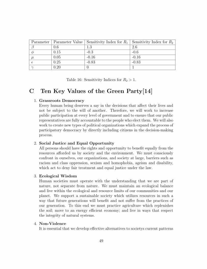
Parameter Parameter Value Sensitivity Index for R1 Sensitivity Index for R2

β 0.6 1.3 2.6φ 0.15 -0.3 -0.6µ 0.05 -0.16 -0.16ε 0.25 -0.83 -0.83γ 0.20 0 1

Table 16: Sensitivity Indices for R2 > 1.

C Ten Key Values of the Green Party[14]

1. Grassroots DemocracyEvery human being deserves a say in the decisions that affect their lives andnot be subject to the will of another. Therefore, we will work to increasepublic participation at every level of government and to ensure that our publicrepresentatives are fully accountable to the people who elect them. We will alsowork to create new types of political organizations which expand the process ofparticipatory democracy by directly including citizens in the decision-makingprocess.

2. Social Justice and Equal OpportunityAll persons should have the rights and opportunity to benefit equally from theresources afforded us by society and the environment. We must consciouslyconfront in ourselves, our organizations, and society at large, barriers such asracism and class oppression, sexism and homophobia, ageism and disability,which act to deny fair treatment and equal justice under the law.

3. Ecological WisdomHuman societies must operate with the understanding that we are part ofnature, not separate from nature. We must maintain an ecological balanceand live within the ecological and resource limits of our communities and ourplanet. We support a sustainable society which utilizes resources in such away that future generations will benefit and not suffer from the practices ofour generation. To this end we must practice agriculture which replenishesthe soil; move to an energy efficient economy; and live in ways that respectthe integrity of natural systems.

4. Non-ViolenceIt is essential that we develop effective alternatives to societys current patterns

49

of violence. We will work to demilitarize, and eliminate weapons of massdestruction, without being naive about the intentions of other governments.We recognize the need for self-defense and the defense of others who are inhelpless situations. We promote non-violent methods to oppose practices andpolicies with which we disagree, and will guide our actions toward lastingpersonal, community and global peace.

5. DecentralizationCentralization of wealth and power contributes to social and economic injus-tice, environmental destruction, and militarization. Therefore, we support arestructuring of social, political and economic institutions away from a systemwhich is controlled by and mostly benefits the powerful few, to a democratic,less bureaucratic system. Decision-making should, as much as possible, remainat the individual and local level, while assuring that civil rights are protectedfor all citizens.

6. Community Bases Economics and Economic JusticeWe recognize it is essential to create a vibrant and sustainable economic sys-tem, one that can create jobs and provide a decent standard of living for allpeople while maintaining a healthy ecological balance. A successful economicsystem will offer meaningful work with dignity, while paying a living wagewhich reflects the real value of a persons work.

Local communities must look to economic development that assures protectionof the environment and workers rights; broad citizen participation in planning;and enhancement of our quality of life. We support independently owned andoperated companies which are socially responsible, as well as co-operativesand public enterprises that distribute resources and control to more peoplethrough democratic participation.

7. Feminism and Gender EquityWe have inherited a social system based on male domination of politics andeconomics. We call for the replacement of the cultural ethics of dominationand control with more cooperative ways of interacting that respect differencesof opinion and gender. Human values such as equity between the sexes, inter-personal responsibility, and honesty must be developed with moral conscience.We should remember that the process that determines our decisions and ac-tions is just as important as achieving the outcome we want.

8. Respect for DiversityWe believe it is important to value cultural, ethnic, racial, sexual, religious and

50

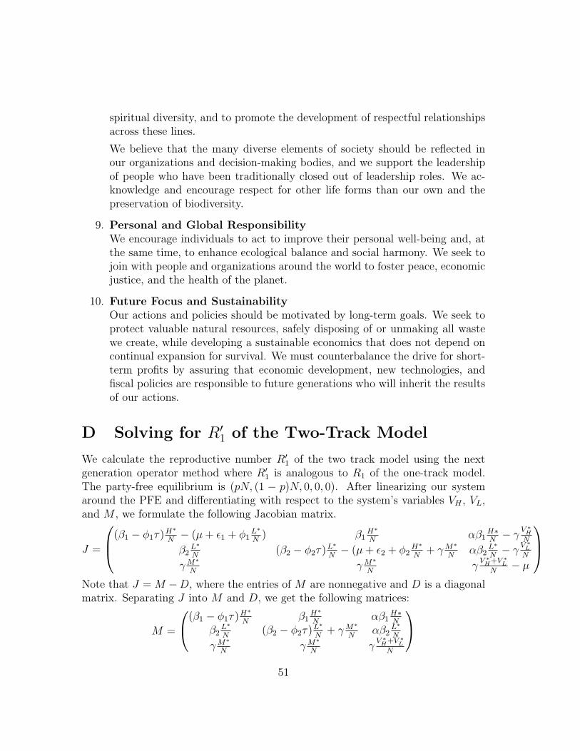
spiritual diversity, and to promote the development of respectful relationshipsacross these lines.

We believe that the many diverse elements of society should be reflected inour organizations and decision-making bodies, and we support the leadershipof people who have been traditionally closed out of leadership roles. We ac-knowledge and encourage respect for other life forms than our own and thepreservation of biodiversity.

9. Personal and Global ResponsibilityWe encourage individuals to act to improve their personal well-being and, atthe same time, to enhance ecological balance and social harmony. We seek tojoin with people and organizations around the world to foster peace, economicjustice, and the health of the planet.

10. Future Focus and SustainabilityOur actions and policies should be motivated by long-term goals. We seek toprotect valuable natural resources, safely disposing of or unmaking all wastewe create, while developing a sustainable economics that does not depend oncontinual expansion for survival. We must counterbalance the drive for short-term profits by assuring that economic development, new technologies, andfiscal policies are responsible to future generations who will inherit the resultsof our actions.

D Solving for R′1 of the Two-Track Model

We calculate the reproductive number R′1 of the two track model using the next

generation operator method where R′1 is analogous to R1 of the one-track model.

The party-free equilibrium is (pN, (1 − p)N, 0, 0, 0). After linearizing our systemaround the PFE and differentiating with respect to the system’s variables VH , VL,and M , we formulate the following Jacobian matrix.

J =

(β1 − φ1τ)H∗

N− (µ + ε1 + φ1

L∗

N) β1

H∗

Nαβ1

H∗N− γ

V ∗H

N

β2L∗

N(β2 − φ2τ)L∗

N− (µ + ε2 + φ2

H∗

N+ γ M∗

Nαβ2

L∗

N− γ

V ∗L

N

γ M∗

Nγ M∗

Nγ

V ∗H+V ∗

L

N− µ

Note that J = M −D, where the entries of M are nonnegative and D is a diagonalmatrix. Separating J into M and D, we get the following matrices:

M =

(β1 − φ1τ)H∗

Nβ1

H∗

Nαβ1

H∗N

β2L∗

N(β2 − φ2τ)L∗

N+ γ M∗

Nαβ2

L∗

N

γ M∗

Nγ M∗

Nγ

V ∗H+V ∗

L

N

51

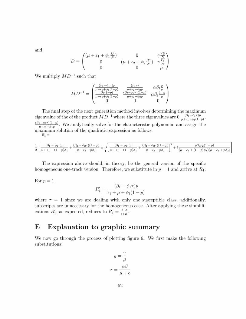
and

D =

(µ + ε1 + φ1L∗

N) 0 γ

V ∗H

N

0 (µ + ε2 + φ2H∗

N) γ

V ∗L

N

0 0 µ

We multiply MD−1 such that

MD−1 =

(β1−φ1τ)p

µ+ε1+φ1(1−p)(β1p)

µ+ε2+φ2pαβ1

pµ

β2(1−p)µ+ε1+φ1(1−p)

(β2−φ2τ)(1−p)µ+ε2+φ2p

αβ21−pµ

0 0 0

The final step of the next generation method involves determining the maximum

eigenvalue of the of the product MD−1 where the three eigenvalues are 0, (β1−φ1τ)pµ+ε1+φ1(1−p)

,(β2−φ2τ)(1−p)

µ+ε2+φ2p. We analytically solve for the characteristic polynomial and assign the

maximum solution of the quadratic expression as follows:R′

1 =

1

2

24 (β1 − φ1τ)p

µ + ε1 + (1− p)φ1+

(β2 − φ2τ)(1− p)

µ + ε2 + pφ2±

s�(β1 − φ1τ)p

µ + ε1 + (1− p)φ1+

(β2 − φ2τ)(1− p)

µ + ε2 + pφ2

�2+ 4

pβ1β2(1− p)

(µ + ε1 + (1− p)φ1)(µ + ε2 + pφ2)

35

The expression above should, in theory, be the general version of the specifichomogeneous one-track version. Therefore, we substitute in p = 1 and arrive at R1:

For p = 1

R′1 =

(β1 − φ1τ)p

ε1 + µ + φ1(1− p)

where τ = 1 since we are dealing with only one susceptible class; additionally,subscripts are unnecessary for the homogeneous case. After applying these simplifi-cations R′

1, as expected, reduces to R1 = β−φε+µ

.

E Explanation to graphic summary

We now go through the process of plotting figure 6. We first make the followingsubstitutions:

y =γ

µ

x =αβ

µ + ε

52

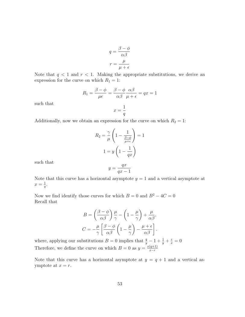
q =β − φ

αβ

r =µ

µ + ε

Note that q < 1 and r < 1. Making the appropriate substitutions, we derive anexpression for the curve on which R1 = 1:

R1 =β − φ

µε=

β − φ

αβ

αβ

µ + ε= qx = 1

such that

x =1

q

Additionally, now we obtain an expression for the curve on which R2 = 1:

R2 =γ

µ

(1− 1

β−φµ+ε

)= 1

1 = y

(1− 1

qx

)such that

y =qx

qx− 1

Note that this curve has a horizontal asymptote y = 1 and a vertical asymptote atx = 1

q.

Now we find identify those curves for which B = 0 and B2 − 4C = 0Recall that

B =

(β − φ

αβ

)µ

γ−(

1− µ

γ

)+

µ

αβ,

C = −µ

γ

[β − φ

αβ

(1− µ

γ

)− µ + ε

αβ

].

where, applying our substitutions B = 0 implies that qy− 1 + 1

y+ r

x= 0

Therefore, we define the curve on which B = 0 as y = x(q+1)x−r

Note that this curve has a horizontal asymptote at y = q + 1 and a vertical as-ymptote at x = r.

53

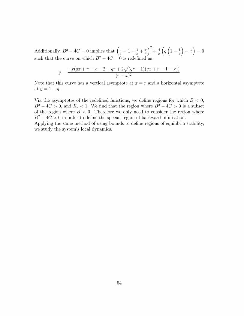
Additionally, B2 − 4C = 0 implies that(

qy− 1 + 1

y+ r

x

)2

+ 4y

(q(1− 1

y

)− 1

x

)= 0

such that the curve on which B2 − 4C = 0 is redefined as

y =−x(qx + r − x− 2 + qr + 2

√(qr − 1)(qx + r − 1− x))

(r − x)2

Note that this curve has a vertical asymptote at x = r and a horizontal asymptoteat y = 1− q.

Via the asymptotes of the redefined functions, we define regions for which B < 0,B2 − 4C > 0, and R2 < 1. We find that the region where B2 − 4C > 0 is a subsetof the region where B < 0. Therefore we only need to consider the region whereB2 − 4C > 0 in order to define the special region of backward bifurcation.Applying the same method of using bounds to define regions of equilibria stability,we study the system’s local dynamics.

54