An estimate of the inﬂation factor and analysis

Nonlin. Processes Geophys., 24, 329–341, 2017https://doi.org/10.5194/npg-24-329-2017© Author(s) 2017. This work is distributed underthe Creative Commons Attribution 3.0 License.

An estimate of the inflation factor and analysis sensitivityin the ensemble Kalman filterGuocan Wu1,2 and Xiaogu Zheng3

1College of Global Change and Earth System Science, Beijing Normal University, Beijing, China2Joint Center for Global Change Studies, Beijing, China3Key Laboratory of Regional Climate-Environment Research for East Asia, Institute of Atmospheric Physics,Chinese Academy of Sciences, Beijing, China

Correspondence to: Guocan Wu ([email protected])

Received: 18 August 2016 – Discussion started: 4 October 2016Revised: 17 May 2017 – Accepted: 26 May 2017 – Published: 3 July 2017

Abstract. The ensemble Kalman filter (EnKF) is a widelyused ensemble-based assimilation method, which estimatesthe forecast error covariance matrix using a Monte Carloapproach that involves an ensemble of short-term forecasts.While the accuracy of the forecast error covariance matrixis crucial for achieving accurate forecasts, the estimate givenby the EnKF needs to be improved using inflation techniques.Otherwise, the sampling covariance matrix of perturbed fore-cast states will underestimate the true forecast error covari-ance matrix because of the limited ensemble size and largemodel errors, which may eventually result in the divergenceof the filter.

In this study, the forecast error covariance inflation factoris estimated using a generalized cross-validation technique.The improved EnKF assimilation scheme is tested on theatmosphere-like Lorenz-96 model with spatially correlatedobservations, and is shown to reduce the analysis error andincrease its sensitivity to the observations.

1 Introduction

For state variables in geophysical research fields, a commonassumption is that systems have “true” underlying states.Data assimilation is a powerful mechanism for estimatingthe true trajectory based on the effective combination of adynamic forecast system (such as a numerical model) andobservations (Miller et al., 1994). Data assimilation providesan analysis state that is usually a better estimate of the statevariable because it considers all of the information provided

by the model forecasts and observations. In fact, the anal-ysis state can generally be treated as the weighted averageof the model forecasts and observations, while the weightsare approximately proportional to the inverse of the corre-sponding covariance matrices (Talagrand, 1997). Therefore,the performance of a data assimilation method relies signifi-cantly on whether the error covariance matrices are estimatedaccurately. If this is the case, the assimilation can be accom-plished with the rapid development of supercomputers (Re-ichle, 2008), although finding the appropriate analysis stateis a much difficult problem when the models are nonlinear.

The ensemble Kalman filter (EnKF) is a practicalensemble-based assimilation scheme that estimates the fore-cast error covariance matrix using a Monte Carlo methodwith the short-term ensemble forecast states (Burgers et al.,1998; Evensen, 1994). Because of the limited ensemble sizeand large model errors, the sampling covariance matrix ofthe ensemble forecast states usually underestimates the trueforecast error covariance matrix. This finding indicates thatthe filter is over reliant on the model forecasts and excludesthe observations. It can eventually result in the divergence ofthe filter (Anderson and Anderson, 1999; Constantinescu etal., 2007; Wu et al., 2014).

The covariance inflation technique is used to mitigate fil-ter divergence by inflating the empirical covariance in EnKF,and it can increase the weight of the observations in the anal-ysis state (Xu et al., 2013). In reality, this method will perturbthe subspace spanned by the ensemble vectors and better cap-ture the sub-growing directions that may not have been cap-tured by the original ensemble (Yang et al., 2015). Therefore,

Published by Copernicus Publications on behalf of the European Geosciences Union & the American Geophysical Union.

330 G. Wu and X. Zheng: An estimate of the inflation factor and analysis sensitivity

using the inflation technique to enhance the estimate accu-racy of the forecast error covariance matrix is increasinglyimportant.

A widely used inflation technique involves multiplying theforecast error matrix by an inflation factor, which must bechosen appropriately. In early studies, researchers usuallytuned the inflation factor by repeated assimilation experi-ments and selected the estimated inflation factor according totheir experience and prior knowledge (Anderson and Ander-son, 1999). However, such methods are very empirical andsubjective. It is not appropriate to use the same inflation fac-tor during all the assimilation procedure. Too small or toolarge an inflation factor will cause the analysis state to overrely on the model forecasts or observations, and can seriouslyundermine the accuracy and stability of the filter.

In later studies, the inflation factor is estimated on-line based on the innovation statistic (observation-minus-forecast; Dee, 1995; Dee and Silva, 1999) with different con-ditions. Moment estimation can facilitate the calculation bysolving an equation of the innovation statistic and its real-ization (Li et al., 2009; Miyoshi, 2011; Wang and Bishop,2003). Maximum likelihood approach can obtain a betterestimate of the inflation factor than moment approach, al-though it must calculate a high-dimensional matrix determi-nant (Liang et al., 2012; Zheng, 2009). Bayesian approachassumes a prior distribution for the inflation factor but is lim-ited by spatially independent observational errors (Anderson,2007, 2009). This study seeks to address the estimation of theinflation factor from the perspective of cross-validation (CV).

The concept of CV was first introduced for linear regres-sions (Allen, 1974) and spline smoothing (Wahba and Wold,1975), and it represents a common approach that can beapplied to estimate tuning parameters in generalized addi-tive models, nonparametric regressions and kernel smooth-ing (Eubank, 1999; Gentle et al., 2004; Green and Silverman,1994; Wand and Jones, 1995). Usually, the data are dividedinto subsets some of which are used for modeling and anal-ysis while others for verification and validation. The mostwidely used technique removes only one data point and usesthe remainder to estimate the value at this point to test theestimation accuracy, which is also called the leave-one-outcross-validation (Gu and Wahba, 1991).

The basic motivation behind CV is to minimize the pre-diction error at the sampling points. The generalized cross-validation (GCV) is a modified form of ordinary CV, thathas been found to possess several favorable properties andis more popular for selecting tuning parameters (Craven andWahba, 1979). For instance, Gu and Wahba (1991) appliedthe Newton’s method to optimize the GCV score with mul-tiple smoothing parameters in a smoothing spline model.Wahba et al. (1995) briefly reviewed the properties of theGCV and conducted an experiment to choose smoothingparameters in the context of variational data assimilationschemes with numerical weather prediction models. Zhengand Basher (1995) also applied the GCV in a thin-plate

smoothing spline model of spatial climate data to deal withSouth Pacific rainfalls.

Actually, the GCV criterion is based on a predictive mean-square-error criterion that attempts to obtain a best estimate(Wahba et al., 1995). It has a rotation-invariant property thatis relative to the orthogonal transformation of the observa-tions and is a consistent estimate of the relative loss (Gu,2002). For the inverse problems in such fields as meteorolog-ical data assimilation, GCV method can choose parameterssystematically by minimizing a given objective function thatwill improve the assimilation results. It can particularly se-lect parameters that reflect not only measurement accuraciesfrom different sources but also model capability (Krakauer etal., 2004).

This study proposes a new method for choosing the infla-tion factor using GCV method. The suitability of this choiceis assessed using a statistic known as the analysis sensi-tivity, which apportions uncertainty in the output to differ-ent sources of uncertainty in the input (Saltelli et al., 2004,2008). In the context of statistical data assimilation, thisquantity describes the sensitivity of the analysis to the ob-servations, which is complementary to the sensitivity of theanalysis to model forecasts (Cardinali et al., 2004; Liu et al.,2009).

This study focuses on a methodology that can be poten-tially applied to geophysical applications of data assimilationin the near future. This paper consists of four sections. Theconventional EnKF scheme is summarized and the improvedEnKF with GCV inflation scheme is proposed in Sect. 2,the verification and validation processes are conducted on anidealized model in Sect. 3, the discussions are presented inSect. 4 and conclusions are given in Sect. 5.

2 Methodology

2.1 EnKF algorithm

For consistency, a nonlinear discrete-time dynamical forecastmodel and linear observation system can be expressed as fol-lows (Ide et al., 1997):

xti =Mi−1

(xai−1)+ ηi, (1)

yoi =Hix

ti + εi, (2)

where i represents the time index; xti =

{xti,1,x

ti,2, . . .,x

ti,n

}T

represents the n-dimensional true state vector at the ith time

step; xai−1 =

{xai−1,1,x

ai−1,2, . . .,x

ai−1,n

}Trepresents the n-

dimensional analysis state vector, which is an estimate ofxti−1; Mi−1 represents a nonlinear dynamical forecast op-

erator such as a numerical weather prediction model; yoi ={

yoi,1,y

oi,2, . . .,y

oi,pi

}Trepresents a pi-dimensional observa-

tion vector; Hi represents the observation operator matrix;and ηi and εi represent the forecast and observation error

Nonlin. Processes Geophys., 24, 329–341, 2017 www.nonlin-processes-geophys.net/24/329/2017/

G. Wu and X. Zheng: An estimate of the inflation factor and analysis sensitivity 331

vectors, which are assumed to be time uncorrelated, statis-tically independent of each other and have mean zero andcovariance matrices Pi and Ri , respectively. The EnKF as-similation result is a series of analysis states xa

i that is anaccurate estimate of the corresponding true states xt

i basedon the information provided by Mi and yo

i .Suppose the perturbed analysis state at a previous time step

xa(j)i−1 has been estimated (1≤ j ≤m and m is the ensemble

size), the detailed EnKF assimilation procedure is summa-rized as the following forecast step and analysis step (Burg-ers et al., 1998; Evensen, 1994).

2.1.1 Step 1: forecast step

The perturbed forecast states are generated by running dy-namical model forward:

xf(j)i =Mi−1

(x

a(j)i−1

). (3)

The forecast state xfi is defined as the ensemble mean of

xf(j)i , and the forecast error covariance matrix is initially es-

timated as the sampling covariance matrix of perturbed fore-cast states:

Pi =1

m− 1

m∑j=1

(x

f(j)i − x

fi

)(x

f(j)i − x

fi

)T. (4)

2.1.2 Step 2: analysis step

The analysis state is estimated by minimizing the followingcost function:

J (x)=(x− xf

i

)TP−1i

(x− xf

i

)+(yoi −Hix

)TR−1i

(yoi −Hix

), (5)

which has the analytic form

xai = x

fi +PiHT

i

(HiPiHT

i +Ri)−1

d i, (6)

where

d i = yoi −Hix

fi (7)

is the innovation statistic (observation-minus-forecast resid-ual in observation space). To complete the ensemble forecast,the perturbed analysis states are calculated using perturbedobservations (Burgers et al., 1998):

xa(j)i = x

f(j)i +PiHT

i

(HiPiHT

i +Ri)−1

(d i + ε

′(j)i

), (8)

where ε′(j)i is a normally distributed random vari-

able with mean zero and covariance matrix Ri . Here,(HiPiHT

i +Ri)−1 can be easily calculated using the

Sherman–Morrison–Woodbury formula (Golub and Loan,1996; Liang et al., 2012; Tippett et al., 2003). Finally, seti = i+ 1, return to Step 1 for the model forecast at the nexttime step and repeat until the model reaches the last time stepN .

2.2 Influence matrix and forecast error inflation

The forecast error inflation procedure should be added toany ensemble-based assimilation scheme to prevent the filterfrom diverging (Anderson and Anderson, 1999; Constanti-nescu et al., 2007). Multiplicative inflation is one of the com-monly used inflation techniques, and it adjusts the initiallyestimated forecast error covariance matrix Pi to λiPi afterestimating the inflation factors λi properly.

In this study, a new procedure for estimating multiplicativeinflation factors λi is proposed based on the following GCVfunction (Craven and Wahba, 1979)

GCVi(λ)=1pidTi R−1/2

i

(Ipi −Ai(λ)

)2R−1/2i d i[

1pi

Tr(Ipi −Ai(λ)

)]2 , (9)

where Ipi is the identity matrix with dimension pi ×pi ;R−1/2i is the square root matrix of Ri ; and

Ai(λ)= Ipi −R1/2i

(HiλPiHT

i +Ri)−1R1/2

i (10)

is the influence matrix (see Appendix A for details).The inflation factor λi is estimated by minimizing the

GCV (Eq. 9) as an objective function, and it is implementedbetween steps 1 and 2 in Sect. 2.1. Then, the perturbed anal-ysis states are modified to

xa(j)i = x

f(j)i + λiPiH

Ti

(HiλiPiHT

i +Ri)−1

(d i + ε

′(j)i

). (11)

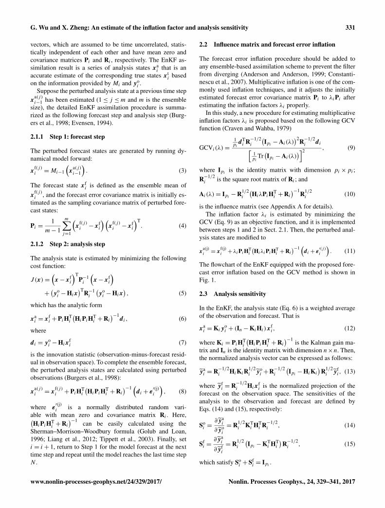
The flowchart of the EnKF equipped with the proposed fore-cast error inflation based on the GCV method is shown inFig. 1.

2.3 Analysis sensitivity

In the EnKF, the analysis state (Eq. 6) is a weighted averageof the observation and forecast. That is

xai =Kiy

oi + (In−KiHi)x

fi, (12)

where Ki = PiHTi

(HiPiHT

i +Ri)−1 is the Kalman gain ma-

trix and In is the identity matrix with dimension n×n. Then,the normalized analysis vector can be expressed as follows:

yai = R−1/2

i HiKiR1/2i yo

i +R−1/2i

(Ipi −HiKi

)R1/2i yf

i, (13)

where yfi = R−1/2

i Hixfi is the normalized projection of the

forecast on the observation space. The sensitivities of theanalysis to the observation and forecast are defined byEqs. (14) and (15), respectively:

Soi =

∂yai

∂yoi

= R1/2i KT

i HTi R−1/2

i , (14)

Sfi =

∂yai

∂yfi

= R1/2i

(Ipi −KT

i HTi

)R−1/2i , (15)

which satisfy Soi +Sf

i = Ipi .

www.nonlin-processes-geophys.net/24/329/2017/ Nonlin. Processes Geophys., 24, 329–341, 2017


a(j)

11; , 1, ,ii j m x

iM

o , ,i i iy R H

T

T f(j) f f(j) f

11

mi

i i i i i i i i i

jm

P H x x H x H x=

T

T f(j) f f(j) f

11

mi

i i i i i i i i i i i i

jm

H PH H x H x H x H x=

a(j) f(j) T T 1 '(j)( )i i i i i i i i i i i i x x P H H P H R d ε?i N

o f

i i id y H xi

=

2T 1/2 1/2

2

1( )

ˆ

1Tr ( )

i

i

i i p i i i

ii

p i

i

pargmin

p

d R I A R d

I A

f f(j)

1

1 m

i i

jm

x x=

f(j) a(j)

1 1i i iM x x=

T

f(j) f f(j) f

1

1

1

m

i i i i i i i

jm

P x x x x P

a f T T 1( )i i i i i i i i i i i x x P H H P H R d

Figure 1. Flowchart of the proposed assimilation scheme.

The elements of the matrix Soi reflect the sensitivity of the

normalized analysis state to the normalized observations; itsdiagonal elements are the analysis self-sensitivities and theoff-diagonal elements are the cross-sensitivities. On the otherhand, the elements of the matrix Sf

i reflect the sensitivity ofthe normalized analysis state to the normalized forecast state.The two quantities are complementary, and the GCV func-tion can be interpreted as minimizing the normalized fore-cast sensitivity because the inflation scheme will increase theobservation weight appropriately.

In fact, the sensitivity matrix Soi is equal to the influence

matrix Ai (see Appendix B for detailed proof), whose tracecan be used to measure the “equivalent number of parame-ters” or “degrees of freedom for the signal” (Gu, 2002; Penaand Yohai, 1991). Similarly, the sensitivity matrix So

i can beinterpreted as a measurement of the amount of informationextracted from the observations (Ellison et al., 2009). Tracediagnostics can be used to analyze the sensitivities to obser-vations or forecast vectors (Cardinali et al., 2004). The globalaverage influence (GAI) at the ith time step is defined as theglobally averaged observation influence:

GAI=Tr(So

i )

pi, (16)

where pi is the total number of observations at the ith timestep.

In the conventional EnKF, the forecast error covariancematrix Pi is initially estimated using a Monte Carlo methodwith short-term ensemble forecast states. However, becauseof the limited ensemble size and large model errors, the sam-pling covariance matrix of perturbed forecast states usuallyunderestimate the true forecast error covariance matrix. Thiswill cause the analysis to over rely on the forecast state andexclude useful information from the observations. This iscaptured by the fact that the GAI values are rather smallfor the conventional EnKF scheme. Adjusting the inflation ofthe forecast error covariance matrix alleviates this problem tosome extent, as will be shown in the following simulations.

2.4 Forecast ensemble spread and analysis RMSE

The spread of the forecast ensemble at the ith step is definedas follows:

Spread=

√√√√ 1n(m− 1)

m∑j=1

∥∥∥xf(j)i − x

fi

∥∥∥2. (17)

Roughly speaking, the forecast ensemble spread is usuallyunderestimated for the conventional EnKF, which also dra-matically decreases until the observations ultimately have an



irrelevant impact on the analysis states. The inflation tech-nique can effectively compensate for the underestimation ofthe forecast ensemble spread, and thereby can improve theassimilation results.

In the following experiments, the “true” state xti is non-

dimensional and can be obtained by a numerical solution ofpartial differential equations. In this case, the distance of theanalysis state to the true state can be defined as the analysisroot mean square error (RMSE), which is used to evaluatethe accuracy of the assimilation results. The RMSE at the ithtime step is defined as follows:

RMSE=

√√√√1n

n∑k=1

(xai,k − xt

i,k

)2. (18)

where xai,k and xt

i,k are the kth components of the analy-sis state and true state at the ith time step. In principle, asmaller RMSE indicates a better performance of the assimi-lation scheme.

3 Numerical experiments

The proposed data assimilation scheme was tested using theLorenz-96 model (Lorenz, 1996) with model errors and a lin-ear observation system as a test bed. The performances of theassimilation schemes described in Sect. 2 were evaluated viathe following experiments.

3.1 Dynamical forecast model and observation systems

The Lorenz-96 model (Lorenz, 1996) is a quadratic nonlin-ear dynamical system that has properties relevant to realisticforecast problems and is governed by the equation

dXkdt= (Xk+1−Xk−2)Xk−1−Xk +F, (19)

where k = 1,2, . . .,40. The cyclic boundary conditionsX−1 = XK−1, X0 = XK and XK+1 = X1 were applied toensure that Eq. (19) is well defined for all values of k.The Lorenz-96 model is “atmosphere-like” because the threeterms on the right-hand side of Eq. (19) are analogous to anonlinear advection-like term, a damping term, and an exter-nal forcing term, respectively. The model can be consideredrepresentative of an atmospheric quantity (e.g., zonal windspeed) distributed on a latitude circle. Therefore, the Lorenz-96 model has been widely used as a test bed to evaluate theperformance of assimilation schemes in many studies (Wu etal., 2013).

The true state is derived by a fourth-order Runge–Kuttatime integration scheme (Butcher, 2003). The time stepfor generating the numerical solution was set at 0.05 non-dimensional units, which is roughly equivalent to 6 h in realtime, assuming that the characteristic timescale of the dis-sipation in the atmosphere is 5 days (Lorenz, 1996). The

forcing term was set as F = 8 so that the leading Lyapunovexponent implies an error-doubling time of approximately 8time steps and the fractal dimension of the attractor was 27.1(Lorenz and Emanuel, 1998). The initial value was chosen tobe Xk = F when k 6= 20 and X20 = 1.001F .

In this study, the synthetic observations were assumed tobe generated by adding random noises that were multivari-ate normally distributed with mean zero and covariance ma-trix Ri to the true states. The frequency was every 4 timesteps, which can be used to mimic daily observations in prac-tical problems, such as satellite data. The observation errorswere assumed to be spatially correlated, which is commonin applications involving remote sensing and radiance data.The variance of the observation at each grid point was set toσ 2

o = 1, and the covariance of the observations between thej th and kth grid points was as follows:

Ri (j,k)= σ 2o × 0.5min{|j−k|,40−|j−k|}. (20)

3.2 Assimilation scheme comparison

Because model errors are inevitable in practical dynamicalforecast models, it is reasonable to add model errors to theLorenz-96 model in the assimilation process. The Lorenz-96model is a forced dissipative model with a parameter F thatcontrols the strength of the forcing. Modifying the forcingstrength F changes the model forecast states considerably.For values of F that are larger than 3, the system is chaotic(Lorenz and Emanuel, 1998). To simulate model errors, theforcing term for the forecast was set to 7, while using F = 8to generate the “true” state. The initially selected ensemblesize was 30.

The Lorenz-96 model was run for 2000 time steps, whichis equivalent to approximately 500 days in realistic problems.The synthetic observations were assimilated at every gridpoint and every 4 time steps using the conventional EnKF,the constant inflated EnKF and the improved EnKF schemesfor comparisons. The time series of estimated inflation fac-tors are shown in Fig. 2. It can be seen that the estimatedinflation factors vary between 1 and 6 in most instances, al-though the values smaller than 1 are estimated in several as-similation time steps. The median of the estimated inflationfactors was 1.88, which was used as the inflation factor inthe constant inflated EnKF scheme. Since the median is a ro-bust and highly efficient statistic of the central tendency, thiscan ensure a relative fair comparison between the constantinflated EnKF and the improved EnKF schemes.

The forecast ensemble spread of the conventional EnKF,constant inflated EnKF and improved EnKF are plotted inFig. 3. For the conventional EnKF, because the forecast statesusually shrink together, the forecast ensemble spread wasquite small and had a mean value of 0.36. The mean spreadvalue of the improved EnKF was 3.32, which was larger thanthat of the constant inflated EnKF (3.25). These findings il-lustrate that the underestimation of forecast ensemble spreadcan be effectively compensated for by the two EnKF schemes



0 500 1000 1500 2000

02

46

810

Time step

Est

imat

ed in

flatio

n fa

ctor

Figure 2. Time series of the estimated inflation factors by minimiz-ing the GCV function. The median of the estimated inflation factorsis 1.88.

EnKFConstant inflated EnKFImproved EnKF

0 500 1000 1500 2000

01

23

45

Time step

Fore

cast

ens

embl

e sp

read

Figure 3. Forecast ensemble spread of the conventional EnKF(black line), the constant inflated EnKF (red line) and the improvedEnKF (blue line) for the Lorenz-96 experiment with 40-observationand 30-ensemble member. The constant multiplicative inflation fac-tor is set as 1.88.

with forecast error inflation and that the improved EnKF ismore effective than the constant inflated EnKF.

To evaluate the analysis sensitivity, the GAI statistics(Eq. 16) were calculated, and the results are plotted in Fig. 4.The GAI value increases from 10 % for the conventionalEnKF to 30 % for the improved EnKF, indicating that thelatter relies more on the observations. This finding is impor-tant because the observations can play a significant role incombining the results with the model forecasts to generatethe analysis state. In addition to small fluctuations, the meanGAI value of the constant inflated EnKF was 27.80 %, whichwas smaller than that of the improved EnKF.


0 500 1000 1500 2000

00.

10.

20.

30.

40.

50.

60.

7

Time step

Valu

e of

GA

I sta

tistic

Figure 4. GAI statistics of the conventional EnKF (black line), theconstant inflated EnKF (red line) and the improved EnKF (blue line)for the Lorenz-96 experiment with 40-observation and 30-ensemblemember. The constant multiplicative inflation factor is set as 1.88.

To evaluate the analysis estimate accuracy, the analysisRMSE (Eq. 18) and the corresponding values of the GCVfunctions (Eq. 9) were calculated and plotted in Figs. 5 and6, respectively. The results illustrate that the analysis RMSEand the values of the GCV functions decrease sharply for thetwo EnKF with forecast error inflation schemes. However,the GCV function and the RMSE values of the improvedEnKF were about 15 % smaller than those of the constantinflated EnKF, indicating that the online estimate methodperforms better than the simple multiplicative inflation tech-niques with a constant value. The correlation coefficient ofthe analysis RMSE and the value of the GCV function at theassimilation time step were approximately 0.76, which indi-cates that the GCV function is a good criterion to estimatethe inflation factor.

The ensemble analysis state members of the conven-tional EnKF, constant inflated EnKF and improved EnKF areshown in Fig. 7, and the results indicate the uncertainty ofthe analysis state to some extent. The true trajectory obtainedby the numerical solution is also plotted. It illustrates that alarger difference occurred between the true trajectory and theensemble analysis state members for the conventional EnKFthan for the improved EnKF and constant inflated EnKF. Inaddition, the analysis state was more consistent with the truetrajectory for the improved EnKF than that for the constantinflated EnKF. Therefore, the GCV inflation can lead to amore accurate analysis state than the simple constant infla-tion.

The time-mean values of the forecast ensemble spread, theGAI statistics, the GCV functions and the analysis RMSEover 2000 time steps are listed in Table 1. These results illus-trate that the forecast error inflation technique using the GCVfunction performs better than the constant inflated EnKF,




0 500 1000 1500 2000

01

23

45

67

Time step

Ana

lysi

s R

MS

E

Figure 5. Analysis RMSE of the conventional EnKF (black line),the constant inflated EnKF (red line) and the improved EnKF (blueline) for the Lorenz-96 experiment with 40-observation and 30-ensemble member. The constant multiplicative inflation factor is setas 1.88.


0 500 1000 1500 2000

010

2030

4050

6070

Time step

Valu

e of

GC

V fu

nctio

n

Figure 6. GCV function values of the conventional EnKF (blackline), the constant inflated EnKF (red line) and the improved EnKF(blue line) for the Lorenz-96 experiment with 40-observation and30-ensemble member. The constant multiplicative inflation factor isset as 1.88.

which can indeed increase the analysis sensitivity to the ob-servations and reduce the analysis RMSE.

3.3 Influence of ensemble size and observation number

Intuitively, for any ensemble-based assimilation scheme, alarge ensemble size will lead to small analysis errors; how-ever, the computational costs are high for practical problems.The ensemble size in the practical land surface assimilationproblem is usually several tens of members (Kirchgessner etal., 2014). The preferences of the proposed inflation method

0 500 1000 1500 2000

−10

−50

510

15

Time step

Con

vent

iona

l EnK

F

(a)

0 500 1000 1500 2000

−10

−50

510

15

Time step

Con

stan

t inf

late

d E

nKF

(b)

0 500 1000 1500 2000

−10

−50

510

15

Time step

Impr

oved

EnK

F

(c)

Figure 7. Ensemble analysis state members of the conventionalEnKF (black line), the constant inflated EnKF (red line) and theimproved EnKF (blue line) for the Lorenz-96 experiment with 40-observation and 30-ensemble member. The constant multiplicativeinflation factor is set as 1.88. The green line refers to the true trajec-tory obtained by the numerical solution.

and the constant inflation method with respect to differentensemble sizes (10, 30 and 50) were evaluated, and the re-sults are listed in Table 1. It shows that for each scheme, us-ing a 10-member ensemble produced a 3-fold increase in theanalysis RMSE, while using a 50-member ensemble reducedthe analysis RMSE by 20 % relative to the analysis RMSEobtained using a 30-member ensemble. The forecast ensem-ble spread increased slightly from a 10-member ensembleto a 50-member ensemble. The GAI and GCV function val-ues changed sharply from a 10-member ensemble to a 30-member ensemble, and they became relatively stable from a30-member ensemble to a 50-member ensemble. Ensemblesless than 10 were unstable, and no significant changes oc-curred for ensembles greater than 50. Considering the com-putational costs for practical problems, a 30-member ensem-ble may be necessary for Lorenz-96 model to estimate sta-tistically robust results. In the realistic problem, a system inwhich the errors grow in multiple directions will need moreensembles to produce statistically robust results.



Table 1. Time-mean values of the forecast ensemble spread, GAI statistics, GCV functions and analysis RMSE over 2000 time steps, as wellas the running times (second) for different assimilation schemes. The observation number is 40 and the ensemble size is selected as 10, 30and 50, respectively.

Scheme Ensemble Spread GAI GCV RMSE Runningsize time

Conventional 10 0.23 4.56 % 36.38 4.50 70.73EnKF 30 0.36 10.78 % 31.14 4.01 215.92

50 0.41 13.58 % 25.21 3.52 346.69

Constant 10 3.15 4.78 % 35.91 4.38 77.41inflated 30 3.25 27.48 % 5.56 1.41 238.25EnKF 50 3.27 19.67 % 5.03 1.14 384.63

Improved 10 3.26 5.24 % 35.56 3.74 81.31EnKF 30 3.32 29.21 % 3.29 1.10 251.06

50 3.45 35.63 % 2.30 0.88 405.68

To evaluate the preferences of the inflation method withrespect to different numbers of observations, synthetic ob-servations were generated at every other grid point and forevery 4 time steps. Hence, a total of 20 observations wereperformed at each observation step in this case. The assimi-lation results with ensemble sizes of 10, 30 and 50 are listedin Table 2, which shows that the GAI values were larger thanthose with 40-observations in all assimilation schemes. Thisfinding may be related to the relatively small denominatorof the GAI statistic (Eq. 16) in the 20-observation experi-ments. The forecast ensemble spread does not change muchbut the GCV function and the RMSE values increase greatlyin the 20-observation experiments with respect to those inthe 40-observation experiments, which illustrates that moreobservations will lead to less analysis error.

4 Discussions

4.1 Performance of the GCV inflation

Accurate estimates of the forecast error covariance matrixare crucial to the success of any data assimilation scheme.In the conventional EnKF assimilation scheme, the forecasterror covariance matrix is estimated as the sampling covari-ance matrix of the ensemble forecast states. However, limitedensemble size and large model errors often cause the matrixto be underestimated, which produces an analysis state thatover relies on the forecast and excludes observations. Thiscan eventually cause the filter to diverge. Therefore, the fore-cast error inflation with proper inflation factors is increas-ingly important.

The use of multiplicative covariance inflation techniquescan mitigate this problem to some extent. Several methodshave been proposed in the literature, and each has differentassumptions. For instance, the moment approach can be eas-ily conducted based on the moment estimation of the innova-tion statistic. The maximum likelihood approach can obtain a

more accurate inflation factor than the moment approach, butrequires computing high-dimensional matrix determinants.The Bayesian approach assumes a prior distribution for theinflation factor but is limited to spatially independent obser-vational errors. In this study, the inflation factor was esti-mated based on cross-validation and the analysis sensitivitywas detected. The estimated inflation factor by minimizingthe GCV function is not affected by the observation unit andcan optimize the analysis sensitivity to the observation.

In fact, the GCV method can evaluate and comparelearning algorithms and represents a widely used statisticalmethod. It can be applied in inverse problems in such fieldsas meteorological data assimilation (Wahba et al., 1995).Specifically, GCV provides a well-characterized method,which can select a regularization parameter by minimizingthe predictive data errors with rotation-invariant in a least-squares solution (MacCarthy et al., 2011). In data assimi-lation research fields, observation data such as in situ ob-servation and remote sensing data are usually from differ-ent sources. GCV is particularly useful for choosing rela-tive parameters that reflect not only measurement accuraciesfrom different sources but also model capability (Krakaueret al., 2004). Apparently, GCV method requires calculatingthe trace of a large matrix, which may be commonly compu-tationally prohibitive for large inverse problems (MacCarthyet al., 2011).

In this study, the GCV concept was adopted for the in-flation factor estimation in the improved EnKF assimilationscheme and was validated with the Lorenz-96 model. Theassimilation results showed that inflating the conventionalEnKF using the factor estimated by minimizing the GCVfunction can indeed reduce the analysis RMSE. Therefore,the GCV function can accurately quantify the goodness of fitof the error covariance matrix. The values of the GCV func-tion obviously decreased in the proposed approach comparedthe conventional EnKF and constant inflated EnKF schemes.The analysis RMSE of the proposed approach was also much



Table 2. Same as in Table 1 but for 20 observations.

Scheme Ensemble Spread GAI GCV RMSE Runningsize time

Conventional 10 0.41 10.77 % 33.64 4.85 67.75EnKF 30 0.59 20.92 % 22.89 4.10 181.27

50 0.68 26.41 % 14.97 3.29 295.92

Constant 10 3.03 11.73 % 33.39 4.64 71.22inflated 30 3.18 30.07 % 17.12 3.92 203.64EnKF 50 3.27 39.51 % 12.74 3.37 322.29

Improved 10 3.33 13.25 % 32.17 4.39 74.84EnKF 30 3.36 35.09 % 14.99 3.46 213.81

50 3.48 41.28 % 5.19 2.86 339.41

smaller than those of the conventional EnKF and constant in-flated EnKF schemes, which suggests that the GCV criterionworks well for estimating the inflation factor.

The analysis sensitivities in the proposed approach and inthe conventional EnKF scheme were also investigated in thisstudy. The time-averaged GAI statistic increases from about10 % in the conventional EnKF scheme to about 30 % us-ing the proposed inflation method. This illustrates that theinflation mitigates the problem of the analysis depending ex-cessively on the forecast and excluding the observations. Therelationship of the analysis state to the forecast state and theobservations are more reasonable.

4.2 Computational cost

The highest computational cost when minimizing the GCVfunction is related to calculating the influence matrix Ai(λ).Since the matrix multiplication is commutative for the trace,the GCV function can be easily re-expressed as follows:

GCVi(λ)=pid

Ti

(HiλPiHT

i +Ri)−1Ri

(HiλPiHT

i +Ri)−1

d i[Tr((

HiλPiHTi +Ri

)−1Ri)]2 . (21)

Because both the numerator and denominator of the GCVfunction are scalars, the inverse matrix is needed onlyin(HiλPiHT

i +Ri)−1, which can be effectively calculated

using the Sherman–Morrison–Woodbury formula. Further-more, the inverse matrix calculation and the multiplicationprocess are also indispensable for the conventional EnKF(Eq. 6). Essentially, no additional computational burden isassociated with the improved EnKF for the inverse matrix.Therefore, the total computational costs of the improvedEnKF are feasible.

For the Lorenz-96 experiments in this study, the conven-tional EnKF, constant inflated EnKF and proposed improvedEnKF assimilation schemes were conducted using R lan-guage on a computer with Intel Core i5 CPU and 8 GB RAM.The running times with different observation numbers andensemble sizes were listed in Tables 1 and 2. It shows that for

each assimilation scheme, the computational cost increasesas the ensemble size grows. For the fixed observation num-ber and ensemble size, the conventional EnKF, which doesnot involve the forecast error inflation, has the least run-ning time but at a cost of losing assimilation accuracy. Theproposed EnKF scheme is about 15 % smaller in analysisRMSE, but only about 5 % longer in running time than theconstant inflated EnKF scheme. For the operational meteoro-logical/ocean models, the most computational cost is in theensemble model integrations (Ravazzani et al., 2016). There-fore, the proposed EnKF scheme does not significantly in-crease computational cost.

4.3 Notes

It is worth noting that the inflation factor is assumed to beconstant in space in this study, which may be not the casein realistic assimilation problems. Forcing all components ofthe state vector to use the same inflation factor could sys-tematically overinflate the ensemble variances in sparsely ob-served areas, especially when the observations are unevenlydistributed. In the presence of sparse observations, the statethat is not observed can be improved only by the physicalmechanism of the forecast model, although this improvementis limited. Therefore, a multiplicative inflation may not besufficiently effective to enhance the assimilation accuracy. Inthis case, the additive inflation and the localization techniquecan be applied to further improve the assimilation qualityin the presence of sparse observations (Miyoshi and Kunii,2011; Yang et al., 2015).

5 Conclusions

In this study, the approach for using GCV as a metric to es-timate the covariance inflation factor was proposed. In thecase studies conducted in Sect. 3, the observations were rela-tively evenly distributed and the assimilation accuracy couldindeed be improved by the forecast error inflation technique.These findings provide insights on the methodology and val-



idation of the Lorenz-96 model and illustrate the feasibilityof our approach. In the near future, methods of modifyingthe adaptive procedure to suit the system with unevenly dis-tributed observations and applying to more sophisticated dy-namic and observation systems will be investigated.

Data availability. No data sets were used in this article.



Appendix A

From Eq. (2), the normalized observation equation can bedefined as follows:

yoi = R−1/2

i Hixti + εi, (A1)

where yoi = R−1/2

i yoi is the normalized observation vector

and εi ∼N(0,I); Ipi is the identity matrix with the dimen-sions pi ×pi . Similarly, the normalized analysis vector isyai = R−1/2

i Hixai and the influence matrix Ai relates the nor-

malized observation vector to the normalized analysis vector,thereby ignoring the normalized forecast state in the obser-vation space (Gu, 2002):

yai −R−1/2

i Hixfi = Ai

(yoi −R−1/2

i Hixfi

). (A2)

Because the analysis state xai is given by Eq. (5), the influ-

ence matrix Ai can be verified as follows:

Ai = Ipi −R1/2i

(HiPiHT

i +Ri)−1R1/2

i . (A3)

If the initial forecast error covariance matrix is inflated asdescribed in Sect. 2.2, then the influence matrix is treated asthe following function of λ

Ai(λ)= Ipi −R1/2i

(HiλPiHT

i +Ri)−1R1/2

i , (A4)

The principle of CV is to minimize the estimated error at theobservation grid point. Lacking an independent validationdata set, a common alternative strategy is to minimize thesquared distance between the normalized observation valueand the analysis value while not using the observation on thesame grid point, which is the following objective function:

Vi(λ)=1pi

pi∑k=1

(yoi,k −

(R−1/2i Hix

a[k]i

)k

)2, (A5)

where xa[k]i is the minima of the following “delete-one” ob-

jective function:(x− xf

i

)T(λPi)−1

(x− xf

i

)+(yoi −Hix

)T−k

R−1/2i,−k

(yoi −Hix

)−k. (A6)

The subscript −k indicates a vector (matrix) with its kth el-ement (kth row and column) deleted. Instead of minimizingEq. (A6) pi times, the objective function (Eq. A5) has an-other more simple expression (Gu, 2002):

Vi(λ)=1pi

pi∑k=1

(yoi,k −

(R−1/2i Hix

ai

)k

)2

(1− ak,k

)2 , (A7)

where ak,k is the element at the site pair (k, k) of the influ-ence matrix Ai(λ). Then, ak,k is substituted with the average1pi

pi∑k=1

ak,k =1pi

Tr(Ai(λ)) and the constant is ignored to ob-

tain the following GCV statistic (Gu, 2002):

GCVi(λ)=1pidTi R−1/2

i

(Ipi −Ai(λ)

)2R−1/2i d i[

1pi

Tr(Ipi −Ai(λ)

)]2 . (A8)

Appendix B

The sensitivities of the analysis to the observation are definedas follows:

Soi =

∂yai

∂yoi

= R1/2i KT

i HTi R−1/2

i , (B1)

Substitute the Kalman gain matrix Ki =

PiHTi

(HiPiHT

i +Ri)−1 into So

i , then:

Soi = R1/2

i KTi HT

i R−1/2i

= R1/2i

(HiPiHT

i +Ri)−1HiPiHT

i R−1/2i

= R1/2i

(HiPiHT

i +Ri)−1 (HiPiHT

i +Ri −Ri)

R−1/2i

= R1/2i

(HiPiHT

i +Ri)−1 (HiPiHT

i +Ri)

R−1/2i

−R1/2i

(HiPiHT

i +Ri)−1RiR

−1/2i

= Ipi −R1/2i

(HiλPiHT

i +Ri)−1R1/2

i

= Ai . (B2)

Therefore, the sensitivity matrix Soi is equal to the influence

matrix Ai .



Competing interests. The authors declare that they have no conflictof interest.

Acknowledgements. This work is supported by the National Natu-ral Science Foundation of China (grant no. 91647202), the NationalBasic Research Program of China (grant no. 2015CB953703), theNational Natural Science Foundation of China (grant no. 41405098)and the Fundamental Research Funds for the Central Universi-ties. The authors would like to gratefully acknowledge the twoanonymous reviewers and the editor for their constructive com-ments, which helped significantly in improving the quality of thismanuscript.

Edited by: Amit ApteReviewed by: two anonymous referees

References

Allen, D. M.: The relationship between variable selection and dataaugmentation and a method for prediction, Technometrics, 16,125–127, 1974.

Anderson, J. L.: An adaptive covariance inflation error correctionalgorithm for ensemble filters, Tellus A, 59, 210–224, 2007.

Anderson, J. L.: Spatially and temporally varying adaptive covari-ance inflation for ensemble filters, Tellus A, 61, 72–83, 2009.

Anderson, J. L. and Anderson, S. L.: A Monte Carlo implementa-tion of the nonlinear fltering problem to produce ensemble as-similations and forecasts, Mon. Weather Rev., 127, 2741–2758,1999.

Burgers, G., Leeuwen, P. J., and Evensen, G.: Analysis scheme inthe ensemble kalman filter, Mon. Weather Rev., 126, 1719–1724,1998.

Butcher, J. C.: Numerical methods for ordinary differential equa-tions, John Wiley & Sons, Chichester, 425 pp., 2003.

Cardinali, C., Pezzulli, S., and Andersson, E.: Influence – matrixdiagnostic of a data assimilation system, Q. J. Roy. Meteor. Soc.,130, 2767–2786, 2004.

Constantinescu, E. M., Sandu, A., Chai, T., and Carmichael, G. R.:Ensemble-based chemical data assimilation I: general approach,Q. J. Roy. Meteor. Soc., 133, 1229–1243, 2007.

Craven, P. and Wahba, G.: Smoothing noisy data with spline func-tions, Numer. Math., 31, 377–403, 1979.

Dee, D. P.: On-line estimation of error covariance parameters foratmospheric data assimilation, Mon. Weather Rev., 123, 1128–1145, 1995.

Dee, D. P. and Silva, A. M.: Maximum-likelihood estimation offorecast and observation error covariance parameters part I:methodology, Mon. Weather Rev., 127, 1822–1834, 1999.

Ellison, C. J., Mahoney, J. R., and Crutchfield, J. P.: Prediction,Retrodiction, and the Amount of Information Stored in thePresent, J. Stat. Phys., 136, 1005–1034, 2009.

Eubank, R. L.: Nonparametric regression and spline smoothing,Marcel Dekker, Inc., New York, 338 pp., 1999.

Evensen, G.: Sequential data assimilation with a nonlinear quasi-geostrophic model using Monte Carlo methods to forecast errorstatistics, J. Geophys. Res., 99, 10143–10162, 1994.

Gentle, J. E., Hardle, W., and Mori, Y.: Handbook of computa-tional statistics: concepts and methods, Springer, Berlin, 1070pp., 2004.

Golub, G. H. and Loan, C. F. V.: Matrix Computations, The JohnsHopkins University Press: Baltimore, 1996.

Green, P. J. and Silverman, B. W.: Nonparametric Regressionand Generalized Linear Models: A roughness penalty approach,Vol. 182, Chapman and Hall, London, 1994.

Gu, C.: Smoothing Spline ANOVA Models, Springer-Verlag, NewYork, 289 pp., 2002.

Gu, C. and Wahba, G.: Minimizing GCV/GML scores with multiplesmoothing parameters via the Newton method, SIAM Journal onScientific and Statistical Computation, 12, 383–398, 1991.

Ide, K., Courtier, P., Ghil, M., and Lorenc, A. C.: Unified nota-tion for data assimilation operational sequential and variational,J. Meteorol. Soc. Jpn., 75, 181–189, 1997.

Kirchgessner, P., Berger, L., and Gerstner, A. B.: On the choice of anoptimal localization radius in ensemble Kalman filter methods,Mon. Weather Rev., 142, 2165–2175, 2014.

Krakauer, N. Y., Schneider, T., Randerson, J. T., and Olsen, S.C.: Using generalized cross-validation to select parameters ininversions for regional carbon fluxes, Geophys. Res. Lett., 31,L19108, https://doi.org/10.1029/2004GL020323, 2004.

Li, H., Kalnay, E., and Miyoshi, T.: Simultaneous estimation ofcovariance inflatioin and observation errors within an ensembleKalman filter, Q. J. Roy. Meteor. Soc., 135, 523–533, 2009.

Liang, X., Zheng, X., Zhang, S., Wu, G., Dai, Y., and Li, Y.: Max-imum Likelihood Estimation of Inflation Factors on Error Co-variance Matrices for Ensemble Kalman Filter Assimilation, Q.J. Roy. Meteor. Soc., 138, 263–273, 2012.

Liu, J., Kalnay, E., Miyoshi, T., and Cardinali, C.: Analysis sensitiv-ity calculation in an ensemble Kalman filter, Q. J. Roy. Meteor.Soc., 135, 1842–1851, 2009.

Lorenz, E. N.: Predictability – a problem partly solved, Seminar onPredictability, ECMWF: Reading, UK, 1996.

Lorenz, E. N. and Emanuel, K. A.: Optimal sites for supplementaryweather observations simulation with a small model, J. Atmos.Sci., 55, 399–414, 1998.

MacCarthy, J. K., Borchers, B., and Aster, R. C.: Efficientstochastic estimation of the model resolution matrix di-agonal and generalized cross–validation for large geophys-ical inverse problems, J. Geophys. Res., 116, B10304,https://doi.org/10.1029/2011JB008234, 2011.

Miller, R. N., Ghil, M., and Gauthiez, F.: Advanced data assimila-tion in strongly nonlinear dynamical systems, J. Atmos. Sci., 51,1037–1056, 1994.

Miyoshi, T.: The Gaussian approach to adaptive covariance infla-tion and its implementation with the local ensemble transformKalman filter, Mon. Weather Rev., 139, 1519–1534, 2011.

Miyoshi, T. and Kunii, M.: The Local Ensemble Transform KalmanFilter with the Weather Research and Forecasting Model: Exper-iments with Real Observations, Pure Appl. Geophys., 169, 321–333, 2011.

Pena, D. and Yohai, V. J.: The detection of influential subsets inlinear regression using an influence matrix, J. Roy. Stat. Soc., 57,145–156, 1991.

Ravazzani, G., Amengual, A., Ceppi, A., Homar, V., Romero, R.,Lombardi, G., and Mancini, M.: Potentialities of ensemble strate-


https://doi.org/10.1029/2004GL020323

https://doi.org/10.1029/2011JB008234


gies for flood forecasting over the Milano urban area, J. Hydrol.,539, 237–253, 2016.

Reichle, R. H.: Data assimilation methods in the Earth sciences,Adv. Water Resour., 31, 1411–1418, 2008.

Saltelli, A., Tarantola, S., Campolongo, F., and Ratto, M.: Sensitiv-ity Analysis in Practice: A Guide to Assessing Scientific Models,John Wiley & Sons, Chichester, 219 pp., 2004.

Saltelli, A., Ratto, A. M., Anders, T., Campolongo, F., Cariboni,J., Gatelli, D., Saisana, M., and Tarantola, S.: Global SensitivityAnalysis: The Primer. John Wiley & Sons, Ispra, 292 pp., 2008.

Talagrand, O.: Assimilation of Observations, an Introduction, J.Meteorol. Soc. Jpn., 75, 191–209, 1997.

Tippett, M. K., Anderson, J. L., Bishop, C. H., Hamill, T. M., andWhitaker, J. S.: Notes and correspondence ensemble square rootfilter, Mon. Weather Rev., 131, 1485–1490, 2003.

Wahba, G. and Wold, S.: A completely automatic french curve,Commun. Stat., 4, 1–17, 1975.

Wahba, G., Johnson, D. R., Gao, F., and Gong, J.: Adaptive tun-ing of numerical weather prediction models randomized GCVin three- and four-dimensional data assimilation, Mon. WeatherRev., 123, 3358–3369, 1995.

Wand, M. P. and Jones, M. C.: Kernel Smoothing, Chapman andHall, Maryland, 212 pp., 1995.

Wang, X. and Bishop, C. H.: A comparison of breeding and ensem-ble transform kalman filter ensemble forecast schemes, J. Atmos.Sci., 60, 1140–1158, 2003.

Wu, G., Zheng, X., Wang, L., Zhang, S., Liang, X., and Li, Y.: ANew Structure for Error Covariance Matrices and Their AdaptiveEstimation in EnKF Assimilation, Q. J. Roy. Meteor. Soc., 139,795–804, 2013.

Wu, G., Yi, X., Wang, L., Liang, X., Zhang, S., Zhang, X., andZheng, X.: Improving the ensemble transform Kalman filter us-ing a second-order Taylor approximation of the nonlinear ob-servation operator, Nonlin. Processes Geophys., 21, 955–970,https://doi.org/10.5194/npg-21-955-2014, 2014.

Xu, T., Gómez-Hernández, J. J., Zhou, H., and Li, L.: The powerof transient piezometric head data in inverse modeling: An appli-cation of the localized normal-score EnKF with covariance infla-tion in a heterogenous bimodal hydraulic conductivity field, Adv.Water Resour., 54, 100–118, 2013.

Yang, S.-C., Kalnay, E., and Enomoto, T.: Ensemble singular vec-tors and their use as additive inflation in EnKF, Tellus A, 67,26536, https://doi.org/10.3402/tellusa.v67.26536, 2015.

Zheng, X.: An adaptive estimation of forecast error statistic forKalman filtering data assimilation, Adv. Atmos. Sci., 26, 154–160, 2009.

Zheng, X. and Basher, R.: Thin-plate smoothing spline modeling ofspatial climate data and its application to mapping south Pacificrainfall, Mon. Weather Rev., 123, 3086–3102, 1995.


https://doi.org/10.5194/npg-21-955-2014

https://doi.org/10.3402/tellusa.v67.26536

Documents

An estimate of the inﬂation factor and analysis