Embed Size (px)
Citation preview
AD-A255 143 0
AN EVALUATION OF PROPULSORS DTICFOR SEVERAL NAVY SHIPS lEL.ECTE
SSEP 31992
MARK A. HUGEL DB. S. Systems Eng., United States Naval Academy
(1977)
SUBMITTED TO THE DEPARTMENT OF
OCEAN ENGINEE.INGIN PARTIAL FULFILLMENT OF THE REQUIREMENTS
FOR THE DEGREES OFMASTER OF SCIENCE IN NAVAL ARCHITECTURE AND MARINE ENGINEERING
airdMASTER OF SCIENCE IN MECHANICAL ENGINEERING
at theMASSACHUSETTS INSTITUTE OF TECHNOLOGY
June, 1992
0 Mark A. Hugel, 1992. All rights reserved.
The author hereby grants to MIT permission to reproduce and todistribute copies of this thesis document in whole or in part.
Signature of Author _ _ _ _ _ _ __,
" I Department of Ocean Engineering
May,1992
Certified by , tJ..- /a., C "H•,• AA. Douglas Carmichael
Thesis Supervisor
Certified by C G I'J__ _ _
David 1 Wilson
Thesis Reader
Accepted by I~ [ ~ ~ JAcuA. Douglas Carmichael
Department Graduate CommitteeDepartment of Ocean EngIirnPi--
92 9 02 218
Aeea~iior For
AN EVALUATION OF FROPULSORS
FOR SEVERAL, NAVY SHIPS _D`Fit H but. ten,.'
bbý Codoa
MARK A. HUGEL AVl /IDlst 9pocial
Submitted to the Department of Ocean Engineeringon May 8, 1992 in partial fulfillment of the .
requirements for the Degrees of Master of Science inNaval Architecture and Marine Engineering endMaster of Science in Mechanical Engineering IP_ QUA=• MPEMM, D I
ABSTRACT
A project was undertaken to develop a relatively simple computer program which modelsthe performance, weight, volume and cost of various combinations of propulsion plantcomponents for three different naval ship types. Within that computer program, thetypes of propulsors from which the user may select include fixed pitch propellers,controllable reversible pitch propellers, contrarotating propellers, propeller/pre-swirlvane combinations, and waterjets. The propeller choices include both ducted andnon-ducted configurations. To model these propulsors in a computer program, routineswere developeo to select the correct propulsor geometry to transmit developedhorsepower to the water, &nd to predict the off-design performance, weight and (ifapplicable) volume of the propulsors chosen.Propeller geometry design and off-design performance for the propeller variants werecharacterized using the Propellei Lifting Line computer program developed at MIT.Waterjet performance was predicted using information obtained for KaMeWa waterjets.Correlations describing optimum propelier geometry versus thrust coefficient, propulsorperformance versus ship speed, propulsor weights and volumes were developed for thedifferent ship types. These correlations ame invoked within the propulsor modellingroutines in the program, thereby ailowing the propulsors to be matched with variousengine and transmission combinations. The computer program logic is outlined which isused to match the size and performance oi the chosen propulsion components with a hullsized to tnvelope the proprision plant and a fixed payload. Details are included todescribe the workings of the propulsor model included in the program, and specificdifferences between the destroyer and amphibious ship propulsor models are discussed.Results of the propulsor routines used in the program are graphed for these two shipsallowing a comparison of propulsor types for various ship displacements.
Thesis Supervisor: Dr. A. Douglas CarmichaelTitle: Professor of Power Engineering
2

Acknowledgments
The author would like to thank several people who provided assistance
during the course of this project.
Dr. A. Douglas Carmichael conceived the project and awoke many nights with
inspiring ideas to guide this effort. His insight proved invaluable and his patience
was immeasurable.
Dr. Justin E. Kerwin provided access to the computer modelling tool, and assisted
greatly in ensuring that realistic propeller design results were obtained. He also
patiently answered many questions during the past sevelal months. He and Dr.
Ching - Yeh Hsin were, gracious enough to provide access to the supercomputer
propeiler design account, only to have the author crash the system during its use.
Finally, a special thanks to Luana, Joshua and Chelsea, who helped to provide a
good balance between being a student, husband and father. Their love and support
were ever present.
3
5 Table of Contents
hChapter One ................................................ 8
Introduction ............................................................ 8Background ............................................................. 9
Project Overview ....................................................... 11
Propulsor Evaluation ....................................................... 13
Chapter Two ............................................... 17Using PLL to Predict Propeller Performance ................................. 17
A Description of PLL ...................................................... 17
Generating Wake Velocity Files for Use by PLL ................................ 19
Generating PLL Input Piles for the Different Ship Types ......................... 21
Correlating PLL Designed Propellers to Realistic Cavitation Performance ........... 23
Propeller Design Performance ............................................. 30
-Chapter Three .............................................. 35I Impacts of Propulsor Off-design Performance ............................... 35
Impact of Propulsor Off-design Performance on Sizing the Geosim Ship ............ 353 Impact of Propulsor Off-design Performance on Ship Annual Operating Costs.......39
Using PLL to Predict Propeller Off-design Performance ....................... 40
Tools Available to Predict Propeller Off-design Performance ...................... 40
I Using PLL to Predict Off-design Performance of Propellers with Fixed Pitch ........ 42
Predicting Off-design Performance for Controllable Pitch Propellers ............... 44
Chapter Four .............................................. 49Impact of Propulsor Selection on Propulsion Group Volume and Weight ......... 49
SChapter Five ............. ......... 53The Application of Waterjet Propulsion to Large Surface Combatants ............ 53
W aterjet Perform ance ...................................................... 55
Waterjet Weight and Volume Impact on Ship Design ............................ 56
Chapter Six .............................................. 59
An Outline of the Propulsion Plant Component Assessment ComputerM odel ............................................................. 59
User Selection of Propulsion Components ...................................... 60
4
Matching the Power Plant to the Geosim Ship .................................. 61
Calculating the Acquisition Costs of the Power Plant ............................ 62
Calculating Annual Operating Costs .......................................... 63
Providing Cost and Performance Infomiation ......................... 64
Structure of the Propulsor Module ......................................... 64
The Prop-Design Function .................................................. 65
The PropPerform ance Function .............................................. 66
The Prop-Size Function ..................................................... 71
-Chapter Seven ............................. 73
Conclusions ........................................................... 73
Recommendations for Further Work ....................................... 74
References .................... ............ 76
Appendix One ..................... ....... 79
PLL W ake Files ........................................................ 79
Appendix Two ........................... 82PLL Input Files ........................................................ 82
Appendix Three ............................................ 85
Destroyer Propeller Design Performance .................................... 85
Appendix Four ............................................. 94Amphibious Ship Propeller Design Performance ............................. 94
Appendix Five .............................................. 97
Submarine Propeller Design Performance ................................... 97
Appendix Six ............................................... 99
Destroyer Propeller Off-design Performance ................................. 99
Appendix Seven ........................................... 108Amphibious Ship Propeller Off-design Performance ......................... 108
Appendix Eight ............................................ 111Submarine Propeller Off-design Performance ............................... 111
Appendix Nine ............................................ 113
Controllable Reversible Pitch Propeller Performance During Constant Speed/ Varying Pitch Operation ............................................ 113
Appendix Ten ............................................. 115
W aterjet Perform ance .................................................. 115
5
Appendix Eleven ........................................... 117Computer Routines for Selecting Optimum Propeller Geometry ................ 117
PropDesign for Destroyer Design ........................................... 117
PropDesign for Amphibious Ship Design .................................... 19
Appendix Twelve ........................................... 121Determination of Propeller Diameter for Three Propeller Destroyer ............. 121
Appendix Thirteen ......................................... 124
Computer Routines for Predicting Off-design Propulsor Performance ........... 124
PropPerformance for Destroyer Design ...................................... 124
Prop-Performance for Amphibious Ship Design ................................ 135
Appendix Fourteen ................... ...................... 139Computer Routines for Predicting Propulsor Size and Weight ................. 139
List id Eiur
Figure I - Matrix of Ship Types and Propulsion System Components ........... 12
Figure 2.1 - Cavitation "Bucket" with Optimum Operating Point ............... 24
Figure 2.2 - Cavitation "Bucket" with Typical Operating Regime .............. 25
Figure 2.3 - Burrill Correlation for DDG-51 Data ............................ 27
Figure 2.4 - CT vs Efficiency for a Destroyer ................................ 33
Figure 2.5 - CT vs Efficiency for an Amphibious Ship ........................ 33
Figure 2.6 - CT vs Efficiency for a Submarine ............................... 34
Figure 6.1 - CT vs Propulsive Coefficient for an Amphibious Ship .............. 69
Figure 6.2 - CT vs Propulsive Coefficient for a Destroyer ..................... 70
Figure A3.1 - CT vs Efficiency, J, EAR and P/D for a Destroyer FPP ............ 86
Figure A3.2 - CT vs Efficiency, J, EAR and P/D for a Destroyer CRPPropeller ..................................................... ..... 87
Figure A3.3 - C1,. vs Efficiency, J, EAR and P/D for a DestroyerContrarotating Propeller ........................................ ..... 88
Figure A3.4 - CT vs Efficiency, J, EAR and P/D for a DestroyerFPP/Preswirl Stator Combination ..................................... 89
Figure A3.5 - CT vs Efficiency, J, EAR and P/D for a Destroyer Ducted FPP ..... 90
6
UI
Figure A3.6 - CT vs Efficiency, J, EAR and P/D for a Destroyer Ducted CRPPropeller ..................................................... ..... 91
Figure A3.7 - q, vs Efficiency, J, EAR and P/D for a Destroyer Ducted3 Contrarotating Propeller ........................................ ..... 92Figure A3.8 - CT vs Efficiency, J, EAR and P/D for a Destroyer Ducted
FPP/Preswirl Stator Combination ................................ ..... 93I3 Figure A4.1 - CT vs Efficiency, J, EAR and P/D for an Amphibious Ship
FPP ......................................................... ..... 95Figure A4.2 - CT vs Efficiency, J, EAR and P/D for an Amphibious ShipI CRP Propeller ................................................ ..... 96Figure A5.1 - CT vs Efficiency, J, EAR and P/D for a Submarine
Contrarotating Propeller ........................................ ..... 98Figure A6.1 - Speed vs Efficiency for a Destroyer FPP ...................... 100Figure A6.2 - Speed vs Efficiency for a Destroyer CRP Propeller ............. 101
Figure A6.3 - Speed vs Efficiency for a Destroyer Contrarotating Propeller ..... 102
Figure A6.4 - Speed vs Efficiency for a Destrwyer FPP/Preswirl Stator ......... IC3
Figure A6.5 - Speed vs Efficiercy for a Destroyer Ducted FPP ................ 104
Figure A6.6 - Speed vs Efficiency for a Destroyer Ducted CRP Propeller ....... 1053 Figure A6.7 - Speed vs Efficiency for a Destroyer Ducted ContrarotatingPropeller ..................................................... .... 106
Figure A6.8 - Speed vs Efficiency for a Destroyer Ducted FPP/PreswirlStator ....................................................... .... 107
Figure A7.1 - Speed vs Efficiency for an Amphibious Ship CRP Propeller ...... 109
3 Figure A7.2 - Speed vs Efficiency for an Amphibious Ship CRP Propeller ...... 110
Figure A8.1 -Speed vs Efficiency for a Submarine Contrarotating Propeller .... 112
Figure A9.1 - Normalized Efficiency vs Speed for a CRP Propeller ............ 114
Figure A10.1 - Speed vs Propulsive Coefficient for Destroyer Waterjet ......... 116IIII
*

UU* Chapter One
i Introductiona
1 The design of a naval warship involves a complex and iterative cycle of
decisions and tradeoffs. In order to begin the process, choices of the desired
I payload, size, maneuvering characteristics and eventual cost are a few of many
£ that must be made to assure that the design team is apprised of the objectives,
requirements, philosophy and constraints of the design effort. Another important
decision which must be made early in formulating the foundation of the design is
3 the selection of technologies which are to be included during the design process.0')
Many propulsion technologies have been, and are being, employed on naval
warships, and many more have been proposed. Selection of propulsion
technologies must be made early in the design process, as changing technologies
later in the process would have too large an impact on the design to be feasible. A
method of modelling the available technologies would facilitate comparative
assessments and would promote the chance of choosing the best propulsion plant
for a new design correctly. This paper describes a portion of a larger project
whose goal is to provide a computer model of propulsion plant technologies to aid
* 8

ithe process of selecting competing technologies during the conceptual stages of
the design of several naval ships.
SBackglound
In some areas of ship design (notably portions of the combat system suite)
it is desirable to loosely define desired technologies in the very ealy stages of the
design since the state-of-the-art for many combat systems components can
dramatically change during the several years from design conception to physical
construction. For other areas of ship design (such as the hull form and propulsion
plant) technology choices must be made early in the process, and little or no
flexibility exists in changing ihese choices at any time later in the design, because
of the impact that these systems and their components have on the entire design.
With so nmuch dependent on making the "best" selection of technologies for
incorporation into these high impact systems at the very beginning of a several
year design and construction effort, a means to select the "best" technologies
based in quantitative analysis rather than subjective selection would improve the
likelihood of making the correct choices.
In today's political and economic environment, the emphasis on what is
important in naval ship design has shifted within the past year from obtaining
9
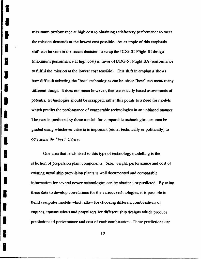
UI3 maximum performance at high cost to obtaining satisfactory performance to meet
the mission demands at the lowest cost possible. An example of this emphasis
I shift can be seen in the recent decision to scrap the DDG-51 Flight III desigii
3 (maximum performance at high cost) in favor of DDG-51 Flight IA (performance
to fulfill the mission at the lowest cost feasible). This shift in emphasis shows
how difficult selecting the "best" technologies can be, since "best" can mean many
-I different things. It does not mean however, that statistically based assessments of
3i potential technologies should be scrapped; rather this points to a need for models
u which predict the performance of comparable technologies in an unbiased manner.
The results predicted by these models for comparable technologies can then be
SI graded using whichever criteria is important (either technically or politically) to
1 determine the "best" choice.
3 One area that lends itself to this type of technology modelling is the
selection of propulsion plant components. Size, weight, performance and cost of
existing naval ship propulsion plants is well documented and comparable
I information for several newer technologies can be obtained or predicted. By using
I these data to develop correlations for the various technologies, it is possible to
build computer models which allow for choosing different combinations of
engines, transmissions and propulsors for different ship designs which produce
I predictions of performance and cost of each combination. These predictions can
10
U
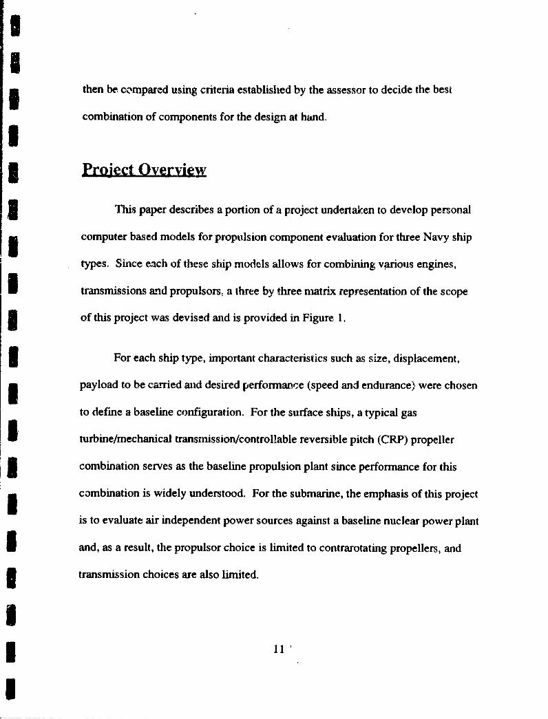
then be. compared using criteria established by the assessor to decide the best
combination of components for the design at hand.U3Project Overview
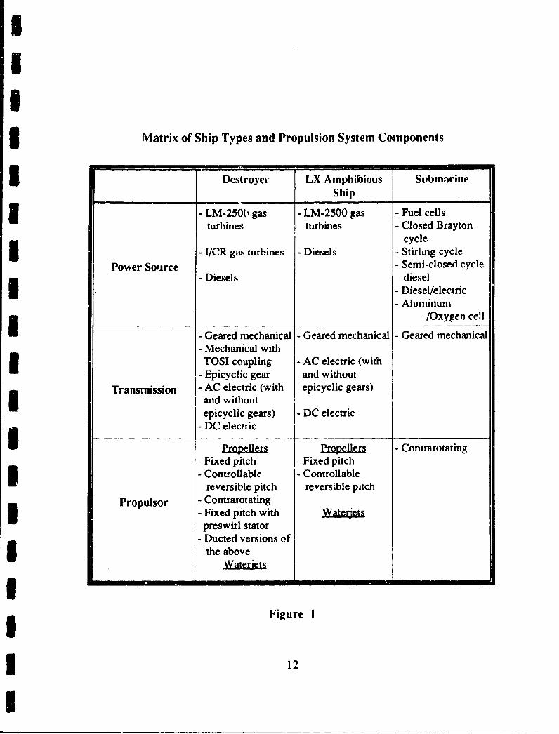
This paper describes a portion of a project undertaken to develop personal
computer based models for propulsion component evaluation for three Navy ship
types. Since each of these ship models allows for combining various engines,
transmissions and propulsors, a three by three matrix representation of the scope
of this project was devised and is provided in Figure 1.
For each ship type, important characteristics such as size, displacement,
payload to be carried and desired performance (speed and endurance) were chosen
to define a baseline configuration. For the surface ships, a typical gas
turbine/mechanical transmission/controllable reversible pitch (CRP) propeller
combination serves as the baseline propulsion plant since performance for this
combination is widely understood. For the submarine, the emphasis of this project
is to evaluate air independent power sources against a baseline nuclear power plant
and, as a result, the propulsor choice is limited to contrarotating propellers, and
transmission choices are also limited.
* 11•
IIIII
3Matrix of Ship Types and Propulsion System Components
Destroyer LX Amphibious SubmarineShip
- LM-250(, gas - LM-2500 gas - Fuel cellsturbines turbines - Closed Brayton
cycle- I/CR gas turbines - Diesels - Stirling cycle
Power Source - Semi-closed cycle- Diesels diesel
- Diesel/electric- Aluminum
i__/Oxygen cell
- Geared mechanical - Geared mechanical - Geared mechanical- Mechanical withTOSI coupling - AC electric (with
- Epicyclic gear and withoutTransmission - AC electric (with epicyclic gears)
i and withoutepicyclic gears) - DC electricI - DC electric
rp_•U P- Contrarotating- Fixed pitch - Fixed pitch3 - Controllable - Controllable
reversible pitch reversible pitch
Propulsor - Contrarotating- Fixed pitch with _Wateriets
preswirl stator- Ducted versions of
the aboveWater lets1-
FigureI
12
U
s Several methods can be employed to assess the impact of propulsor
component variations on a ship design. These include payload fixed or payload
limited and propulsion plant fixed or propulsion plant limited.0) The method
3 employed in this study requires the payload to be fixed, the propulsion system
component types and numbers to be fixed, and then a geometrically similar
(geosim) ship is sized to be as small as possible to contain the payload and power
U plant. The ship endurance is held constant for each propulsion system variation;
this serves as a constant to establish the impact of propulsion efficiency.
I In order to predict operating and life cycle costs, assumptions ha'.'e been
i made regarding the operating profiles of each ship type, other economic factors
(cost estimating methods, discount rates, etc.) and projected number and lifetimes
I of ships to be built. These assumptions are to be applied consistently to each
I component variant taking into account the impact of each variant on volume,
weight, fuel requirements and changes in crew manning.
Propulsor Evaluation
The characterization of the various propulsors listed in Figure 1 involved
choosing a method to predict propulsor efficiency and cavitation performance for
each of the three ship types over a ronge of spec ds, displacements and number of
propulsors in each design. The propeller performance model chosen was the
3 13
U
I
IPropeller Lifting Line (PLL) computer program (developed by Professor J. E.
Kerwin's propeller design group in the Department of Ocean Engineering, MIT).
I This modelling program was chosen because it has the capability to predict
performance for all propeller types included in the project over the range of thrust
and speeds required for each ship type. This program's vortex lattice method of
predicting single propeller performance produces results which are consistent with
U performance predictions for single propellers when applying Lerb's theory (which
produced the most accurate performance predictions of the Mifting line methods).0)
5 It was proposed to detcrmine actuil rather than ideal performance so that
the predictions of the computer program being developed for this project are
re&~istic, and PLL includes features to satisfy this goal. Since PLL has not been
I used for this type of study in the past, it became necessary to correlate PLL
3 propeller designs with some realistic mreasure of cavitation performance (since
ideally PLL designs cavitation-free propeilers). Off-design performance data for
PLL designed propellers was also needed in order to evaluate annual fuel costs for
3 the operating profiles studied.
I Although waterjets have not been used in large naval surface ship
3 applications to this point, there have been proposals that waterjets could be used
for this purpose, particularly in combination with other propulsors. It has been
14
I
I-I shown in some cases, that the lack of appendage drag as a result of using waterjets
more than compensates for higher inefficiencies of waterjets when compared to
I propellers, and a higher propulsive coefficient is attainable.(4) Since no computer
3 model was available to predict waterdet performance, information was obtained
from the Swedish waterjet manufacturer KaMeWa, which is considered to be a
world wide leader in waterjet technology. The waterjet performance information
was correlated in a fashion similar to propeller performance data in order to allow
3 Ifor a fair comparison of results.
3 Weight, volume and cost correlations for propellers and waterjets were
3 included in the propulsor modelling program so that the impact of differences in
these areas could be included within the geosim ship concept described earlier.ITo provide two examples of how the data collected for the various
propulsors is used, the development of the propulsor modules used in the destroyer
5 and amphibious ship power plant models are discussed in this paper. The
3 lpropulsor modules include code for selecting a propeller geometry which is the
most efficient for the required thrust and satisfies cavitation critr ja established
- prior to data collection. Once the geometry is tixed, off-design data correlations
are used to establish propulsive coefficient and propeller rotational speed
3 (revolutions per minute) at maximum speed and cruise speed. Volume, weight
* 15
U

III aand cost correlations are then used to establish the propulsors' contribution to the
geosim ship's size and acquisition cost. Finally, off-design data correlations
i provide predictions of propulsive coefficient and propeller revolutions per minute
3= (rpm) over the operating profile, which are used to determine annual fuel costs for
the combination of propulsion components being assessed.
IIIII,•IIUII
* 16
I
I
* Chapter Two ____
I ]Using PLL to Predict Propeller Perfr nc
A Description of PLL
The use of lifting line theory to model propeller performance has been
3 Ideveloped within the past seventy years, beginning with Prandtl, Betz and
5 Goldstein. Although the early efforts in this area were aimed at modelling high
aspect ratio aircraft propellers, the high aspect ratio assumption had no bearing on
the ability of this method to predict forces on the propeller, which is an important
3 part of preliminary marine propeller design. One drawback in applying lifting line
techniques to propeller design was the large number of tedious calculations
necessary to obtain results. In 1952, Lerbs published the most advanced and
" I accurate of these methods, but without today's computing power available, Lerb's
3theory was not widely applied.(5)
3 More recently, preliminary propeller design using lifting line theory has
u been made feasible by programming the tedious calculations to be performed by
computers. As the computing capabilities have grown, so have the ambitions of
I* 17
U
II
the programmers, resulting in the logical extension of these numerical methods to
multiple component propulsors. While the Lerb's method worked quite well for
I single propellers, the additional desire to model multi-stage and ducted propellers
Swith accuracy comparable to Lerb's theory required developing a computer
program which optimizes blade loading using a lattice of discretized constant
vortex segments. This program, known as the MIT Propeller Lifting Line
I program (PLL), has been developed and refined at MIT over the past six years by
3 Kerwin, Coney and Hsin.(6,7,8,9)
PLL serves as a tool for the preliminary design of propellers. It includes
the capability to model numerous propeller types including
• variable pitch,
contrarotating,
. propeller and pre- or post- swirl stator combinations,
* ducted versions of the above, and
. ringed propellers.
PLL allows the user to vary inputs such as ship speed, propulsor diameter, number
of blades, hub centerline depth, desired thrust (or thrust coefficient) and propeller
rotational speed (or advance coefficient) and then parametrically study the effects
on efficiency, cavitation, strength and cost of the PLL designed propulsor.0'0)
A detailed description of the lifting line theory and vortex lattice methods
18
I
Iemployed by PLL as well as complete details regarding the use of PLL are
provided in reference 10, the PLL User's Manual.I
I Generating Wake Velocity Files for Use by PLL
I In order for PLL to calculate forces induced throughout the vortex lattice
3 representation of the propeller blades, the user is required to provide PLL with
information describing the propeller inflow velocities. This information is
provided in the form of wake files, which are formatted to be read by PLL during
I a PLL design session. Since the wake velocity profiles of the three ships studied
3 during this project were different, separate wake files were generated for each ship
type. These files contain axial, radial and tangential components of the wake field
which are defined in terms of harmonic coefficients of the circumferentially
I varying inflow at specified radii.(') The harmonic coefficients are determined by
3 fitting Fourier cosine and/or sine series curves to the inflow velocities at each
radius.ITo produce the destroyer wake file, a wake velocity file for DDG-51 was
obtained from David Taylor Model Basin. This file contained axial, radial and
I tangential inflow velocities at six different radii gathered during model testing of
the DDG-5 1. This data was plotted, and curve fitting was done using the
19
II
"EasyPlot" plotting computer program to obtain the harmonic coefficients needed
by PLL. The PLL wake file for the destroyer is included in Appendix 1.ITo produce the amphibious ship wake file, a wake velocity file for the
LSD-49 amphibious transport ship was obtained from David Taylor Model Basin.
3 Like the destroyer wake field file, this file contained axial, radial and tangential
3 inflow velocities at six different radii gathered during model testing. These data
were plotted, and the harmonic coefficients obtained by curve fitting these data are
3 included in the PLL wake file for the amphibious ship, which can be found in
3 Appendix 1.
I The PLL wake file for the submarine was constructed using a wake contour
3 diagram for a submarine, which was extracted from the course notes for the MIT
Professional Summer Submarine Design Com-se taught by Captain Harry Jackson,
USN (Ret.). The wake contour diagram was marked at each tenth of a radius from
3 the hub to the tips, and each radius was subdivided into 45 degree increments.
3 The velocity at each radius was then averaged using the velocity at each 45 degree
increment, and these mean velocities were formatted into the PLL submarine wake
I file found in Appendix 1. To verify the accuracy of this method, the Submarine
3 Design Course notes include methods for calculating the wake fraction of a
submarine using correlations based on the hull design. Employing those methods
20
I
Ito a typical, modern nuclear-powered submarine hull resulted in a wake fraction
prediction of 0.637. PLL computes a wake fraction based on the wake file it is
I provided, and the submarine wake file which was generated as described earlier
resulted in a PLL predicted wake fraction of 0.635.
IGenerating PLL Input Files for the Different Ship Types
In addition to information describing the ship's wake velocity field, other
information pertaining to the ship design which affects propeller performance
I must be provided lo PLL. This information includes hub centerline depth,
propeller diameter and (if used) duct dimensions. Therefore, prior to beginning
the propeller design process, predictions of these parameters needed to be made.
j For the twin screw destroyer, the DDG-51 propeller diameter of 17 feet was
chosen for PLL runs, although data related to propeller diameter was collected in
I non-dimensional form using the propeller advance coefficient J defined by
I J = V / (n*Dpp) where V.= speed of advance, ft/secn = shaft rotational speed, revs/sec3D•,OP = propeller diameter, ft.
Hub centerline depths were varied over a range of 15.2 to 17.95 feet, depending
I on the displacement of the ship (four displacements ranging from 8300 to 9500 LT
3 were used). These centerline depths were obtained by running the Advanced Ship
3 21
I
II
Synthesis Evaluation Tool (ASSET) with a DDG-51 input file obtained from
NAVSEA.
The propeller diameter used for amphibious ship propeller design was 16
feet, which matches the diameter of a version of the proposed LX design. Hub
I centerline depth of the LX was known for a 22,700 LT displacement. Tons per
inch immersion (TPI) was calculated using typical amphibious ship hull design
parameters, and this was used to adjust hub centerline depths over the range of
displacements.
IThe diameter selected for the submarine propeller was 18 feet based on
information gathered from the propeller design portion of course notes from the
3I MIT Professional Summer Submarine Design Course. The hub centerline depth
for the submarine propeller was set at 200 feet in order to evaluate propeller
designs against the cavitation criterion described later.IThe dimensions of the ducts (for those propeller designs incorporating
I ducts) were arrived at based on typical duct dimensions described by Coney.('2)
3 Copies of the PLL input files which contain all the parameters discussed above are
included in Appendix 2.
I3 22
I
I
ICorrelating PLL Designed Propellers to Realistic Cavitation PerformanceU
A goal in using PLL for this project was to attempt to predict propulsor
I performance as realistically as possible. With this goal in mind, a limitation in
using PLL is that PLL calculates propeller optimum blade thickness and camber to
produce a propeller which is cavitation-free presuming steady circumferential
inflow at each radius. (As discussed earlier, the wake velocity profile provided to
SI PLL by the user contains velocities which represent the circumferentially averaged
velocities at each control radius.) Blade thickness and camber are optimized by
adjusting them to enable each propeller design to operate at the optimum point on
the associated minmum pressure coefficient versus variation in angle of attack
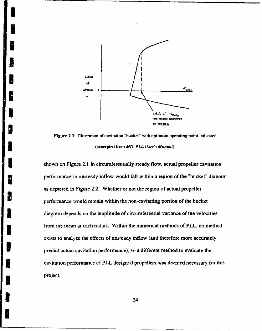
I plot (known as a cavitation "bucket" diagram). Figure 2.1 was excerpted from the
PLL User's Manual to graphically display this idea.
Unfortunately, propellers are normally placed near the stemni of ships where
the wake produced by the ship's hull afkects the inflow velocity field of the
propeller(s). The shafting support struts are also located directly forward of the
I propeller(s), which further disrupts the inflow. The! result is a propeller inflow
3 velocity field which is anything ot, circumferentially steady. as must be assumed
when using the vortex lattice lifting line method in PLL. So, while PLL optimizes
blade thickness and camber to assure that the output propeller operates at the point
I3 23
U
II
I
* ANGLEC
or
A?TACX 0
VA=, or "eCpgFOR V•HIe •E•MTRT
is "TrIMMN
Figure 2 1: Illusmration of cavitation "bucket" with optimum operating point indicated
(excerpted from MIT-PLL User's Manual).
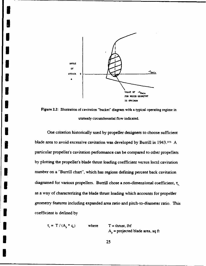
I shown on Figure 2.1 in circumferentially steady flow, actual propeller cavitation
3 Iperformance in unsteady inflow would fall within a region of the "bucket" diagram
as depicted in Figure 2.2. Whether or not the region of actual propeller
Iperformance would remain within the non-cavitating portion of the bucket
3 diagram depends on the amplitude of circumferential variance of the velocities
from thne mean at each radius. Within the numerical methods of PLL, no method
exists to analyze the effects of unsteady inflow (and therefore more accurately
I predict actud cavitation performance), so a different method to evaluate the
cavitation performance cf PLL designed propellers was deemed necessary for this
project.
* 24
U
III
AXGLZ
OrATTA•ICK 0 " ,n
VALM or -cO ,,
FRm VMIOI GZONEThY
Is OP•IIMM
Figure 2.2: Illustration of cavitation "bucket" diagram with a typical operating regime in
unsteady circumferential flow indicated.
One criterion historically used by propeller designers to choose sufficient
3 blade area to avoid excessive cavitation was developed by Burrill in 1943.(13) A
particular propeller's cavitation performance can be compared to other propellers
i by plotting the propeller's blade thrust loading coefficient versus local cavitation
number on a "Burrill chart", which has regions defining percent back cavitation
diagramed for various propellers. Burrill chose a non-dimensional coefficient, ,..
as a way of characterizing the blade thrust loading which accounts for propeller
geometry features including expanded area ratio and pitch-to-diameter ratio. This
coefficient is defined by
r• = T / (Ap*cq) where T = thrust, lbfAP = projected blade area, sq ft
* 25
I
q, = ½6* p..* V,2
V, = relative water velocity at 0.7 tip radius.
The local cavitation number used on a Burrill chart is calculated at 0.7 tip radius
using the following equationIo.• = (p. - p,) / q, where p, - p, = pressure at hub centerline, psi
%q same as defined above.
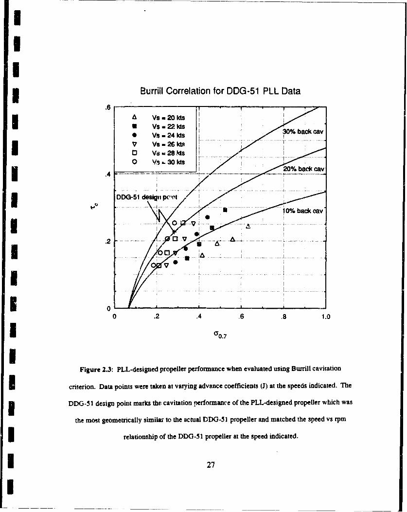
Since the Burrill criterion has been widely used in preliminary propeller
design, and PLL includes all relevant information in its output to determine a PLL
I designed propeller's cavitation peiformance when evaluated using this criterion, it
was chosen as the tool to be used in realistically evaluating potential cavitation
performance. To verify' that this tool would prove useful in comparing PLL
propeller designs, numerous PLL runs were made using speed-power information
I for a DDG-51 while varying ship speed and advance coefficient and then plotting
I the resulting propeller cavitation performance on a Burrill chart. Figure 2.3 shows
that the PLL designs could be easily evaluated using the Burrill criterion, as the
N designs were well separated from each other when plotted on a Burrill chart in this
* method.
Once it was determined that this technique would be useful in comparing
cavitation performance of various PLL desigiis, cavitation performance standards
needed to be established for each of the ship types. For the destroyer and
26
Burrill Correlation for DDG-51 PLL Data.6 0
0 Vs -22OIds
. V-24ts30116back cav
.. .. .. .... ..... .... ..... .. .
3 ODG-51 desigii pcMt
.. ...... ....I. ....
02. 4 ..6 . ... 1.0.....
0 0
Figure 2.3: PLL-designed propeller performance when evaluated using Burrill cavitation
I criterion. Data points were taken at varying advance coefficients (J) at the speeds indicated. The
DDO-5 1 design point marks the cavitation performance of the PLL-designed propeller which was
the most geometrically similar to the actual DDG-51 propeller and matched the speed vs rpm
I relationship of the DDG-51 propeller at the speed indicated.
* 27
!I
amphibious ship, the geometry for the propellers chosen for the respective ship
types was known. It was noted from the PLL output, for example, that the
propeller geometries of the propellers which PLL optimized to operate at 28 knots
3 and 30 knots bounded the geometry of the propeller chosen for ust on DDG-5 1.
3By making several more PLL runs using DDG-51 speed-power information in the
28 to 30 knot regime, the DDG-51 propeller geometry was matched by PLL at 29
N knots ship's speed. This propeller's cavitation performance was plotted on a
Burrill chart (see Figure 2.3) which resulted in 20.7 percent back cavitation. Since
the propeller geometry, rotational speed and thrust produced match the DDG-51
design closely, it was felt that this propeller's cavitation performance must closely
I resemble the cavitation performance of DDG-5 l's propellers, which the Navy
considers satisfactory. Thus, the cavitation standard to be used in evaluating all
other PLL-designed destroyer propellers was established at 20.7 percent back
cavitation while operating at 29 knots ship speed and the corresponding thrust.IIn a similar manner the amphibious ship propeller geometry was matched
using PLL. The Burrill cavitation performance standard for this ship type was
estabhshed at 14.5 percent back cavitation at 23.25 knots ship speed and the
corresponding thrust.
I* 28
I
I
The cavitation stanoard for the submarine propeller was not carried out
using the same method as for the surface ships since actual submarine propeller
geometry information was not available. Instead, it was decided that since the
submarine design was to have a maximum speed of 27 knots, it would be desirable
that the propeller did not cavitate (that is, zero percent back cavitation) up to the
maximum speed when the submarine was submerged with the hub centerline at or
I below 200 feet. PIL runs were then made to assure that this cavitation standard
could be met by contrarotating propellers over the expected range of thrusts. This
standard proved to be feasible, and was therefore adopted.
As stated earlier, realistic cavitation performance predictions were a goal of
the propulsor design, To this end, PLL allows for unloading the propeller hub and
blade tips while optimizing blade loading, which is desirable to minimize sources
of cavitation. This feature was employed to ensure that the propellers designed for
this project using fPLL exhibit the best possible cavitation performance, given that
the tool being used is intended for preliminary propeller design. The effect of hub
I and tip undoading resulted in open water efficiency predictions for the various
propeller designs being several percent less than efficiencies of the same
propwllers with no effort to unload the hub and tips; however, this tradeoff was felt
to be in keeping with the intent of producing realistic performance results.
21 29
I
II
SiPropeller Design Perforwance
I Once the cavitation perfennance standard for each ship type was defined,
3 detennination of satisfactory propeller designs was begun. Since each propulsor
type would be combined with various types and numbers of transmissions and
elgines, the resulting geosim ships could be e.xpected to vary somewhat il size
I and dsplacement from the baseline ship of each type. The variance in
displacements would result in differemt speed-power curves for each geosim ship,
and therefore it became necessary to exercise PLL not oniy to find propeller
designs which satisfied the cavitation criteia, but also which produced a range of
3 thrusts at the design conditions (the design conditions being 29 knots at the
3 corresponding thrust for the DDG, 23.25 knots at the corresponding thrust for the
amphibious ship, and 27 knots at the corresponding thrust foi the submarine).
Once satisfactory propeller designs were generated using PLL, a method
which could be simply programmed to dhoose the most efficient pror.weller
I geometry which produced stifficient thrust was needed. One method offered by
3 IManen (1966) to compare optiraum propulsor efficienries for various types of
propulsors involved comparing open water efficiency versus a non-dirnensional
torque coefficient bq where
3*I 30
I
I
bq= KQ / J. and KQ = propeller torque coefficientJ = propel~ler advance coefficient .(14)
For this project, since thrust, rather than torque, was the variable of interest, a
similar approach to Manen's, comparing open water propeller efficiency versus a
non-dimensional thrust coefficient, was seen as the method to choose the optimum
propeller geometry. The thrust coefficient chosen was CT, where
- Cr =T / (IpwV2AP) and T=thrust,lbf
V. = ship speed, ft/sec"AP = propeller disc area, irDEirp 2 /4.
I Once this method was settled upn, PLL was repeatedly run for the various
pr'peller types of interest. The required thrust was varied and the propeller
designs which 1) satisfied the cavitation performance standard for the ship type,
and 2) showed the optimum open water efficiency, were identified. Propeller
3 designs which had higher efficiencies but did not satisfy the Burrill cavitation
standards for the respective ship type discussed earlier were eliminated from
consideration at this point, so that all possible propeller designs selected from the
remainder were known to meet the cavitation standard developed during this
project. Graphs of the results are presented in Appendix 3 for the DDG propellers,
Appendix 4 for the amphibious ship propellers and Appendix 5 for the submarine
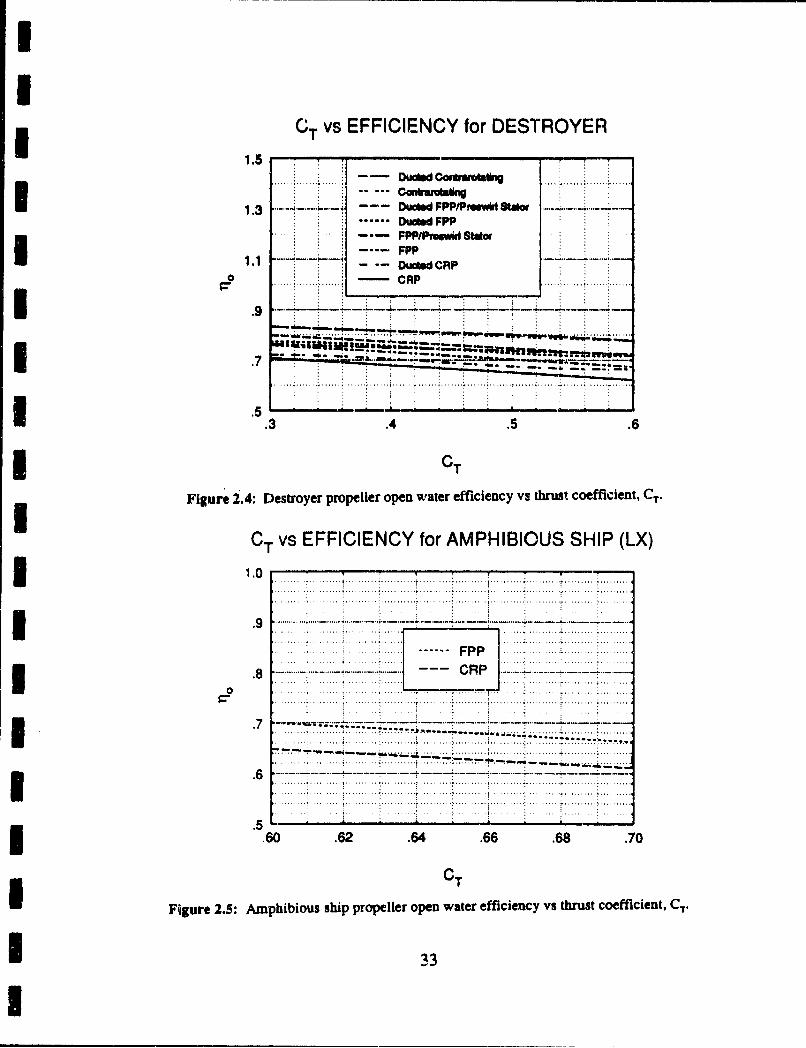
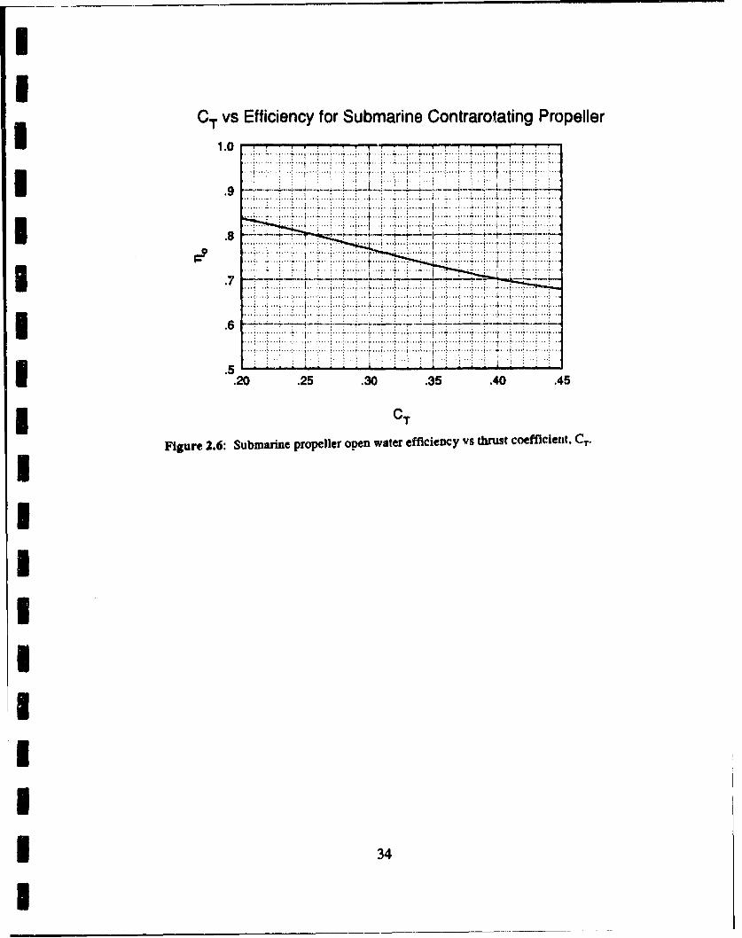
propellers. Comparisons of the design pcrformance of the various propeller types
I being studied for each ship are provided in Figures 2.4, 2.5 -ad 2.6, which depict
*31
open water efficiencies for the various propeller options for the destroyer,
amphibious ship and submarine, respectively. These comparisons show that the
I results of the PLL runs at design conditions are consistent with anticipated
propeller performance; that is, the contrarotating propellers performed at about
seven percent higher efficiency than fixed pitch propellers, propeller-preswirl
stator combinations performed 3-4 percent better, and ducted propellers generally
i performed better than non-ducted versions of the same type.
Included on the graphs in Appendices 3, 4 and 5 are plots of the propeller
geometry characteristics which also vary with changing thrust coefficient. Curves
were fit to the data in these graphs, so that these curve fitting equations provide a
correlation between required thrust and optimum propeller geometry. This
I[ provides the means to select the optimum propeller geometry of a particular
3 propeller type (which exhibits satisfactory cavitation performance) within a
* relatively simple computer program simply by
defining the resistance of the geosim ship at the cavitation design speed,
I • calculating the thrust coefficient based on ship resistance and number ofpropulsors available to generate the required thrust, and
• predicting optimum propeller geometry using the thrust coefficient and therelevant correlation equation.
I Development of the computer program will be discussed later.
* 32
I'
IC vs EFFICIENCY for DESTROYER1.5 -
1.3 ----- - - DUsdWFPP/Pmsww' Sdat....DUCd FPP
FPP/P,'swkl Satdo---- FPP
0 -
** CRP
I .9
.. . ... ... ......uIf ... ... .. .. .. . ...... ..ws w - . W~ .... . .. ..
I -.5.3 .4 .5 .6
3 CTFigure 2.4: Destroyer propeller open water efficiency vs thrut coefficient, CT.
CT vs EFFICIENCY for AMPHIBIOUS SHIP (LX)
1.0 -
1 .9
7.. . . . . . . . . . . . . .. . . ............................. . . . . . . . . . .. .. ...... . . . . ....
S..7 ...I6 ...6... ..6. .6.6.7
.CTFigure...... 2.5:... Am hbou..p.rp.lroe.wtrefiinc..thutcofiiet. T
I...33.... ..... .......I. ... ........
CT vs Efficiency for Submarine Contrarotating Propeller1.0 : : : , -
I .9
*. .. ........
.7 L.6.. .. ..
.............................. .. ...... ..... ,........ ......
.5.
.20 .25 .30 .35 .40 .45
* CT
Figure 2.6: Submarine propeller open water efficiency vs thrust coefficient, CT-.
I3
Chapter Three
Impacts of Propulsor Off-design PerformanceII
Impact of Propulsor Off-design Performance on Sizing the Geosim ShipIAssessing the impact of a particular combination of propulsion components
I on a payload-fixed geosim ship design requires that the weight and volume of the
propulsion plant components, propulsion auxiliaries and propulsion-a3sociated
tankage (hereafter collectively referred to as the propulsion group) be detenmined.
Two performance attributes have the most affect on the weight and volume of the
I propulsion group:
I• attainment of maximum speed as specified in the design objectives, and
attainment of endurance range at cruise speed as specified in the design3 objectives.
Designing to satisfy' these two objectives results in the characterization of
propulsion component size (based on power developed to achieve maximum
I speed) and auxiliary and tankage requirements (based on carrying a sufficient fuel
supply to meet the specified endurance range while the engines power the ship at
1* 35
I
I
cruise speed and the electrical generators produce the power necessary to meet the
24 hour average electrical load).IAssessing a particular propulsor's impact on propulsion group weight and
I volume requires determining the propulsor's capability to take the power
developed in the engines and subsequently delivered to the propulsor via the
transmission and shafting (known as developed horsepower or DHP), and transmit
that power into the water to overcome the resistance of the sea to the hull and its
I appendages (known as effective horsepower or EHP). This capability is known as
the propulsive coefficient of a propulsor and is defined by
(Q)PC = EHP / DHP = I. rlIbullTIwhere io = open water efficiency
Iih.ul = hull efficiency = (l-t) / (l-w)IIRRE = relative rotative efficiencyand t = tf-irust deduction factor
w = wake fraction.
Knowing the propulsive coefficient of a particular propulsor type at high
speed allows predicting the maximum possible ship speed based upon engine
I power installed and EHP necessary to propel the ship at a particular speed. The
rotational speed (typically in revolutions per minute - rpm) of the particular
propulsor at maximum speed must also be found so that the transmission gear ratio
necessary to match maximum engine rpm with propulsor rpm can be determined.
I* 36
I
In this project, since the number of engines, transinissions and propulsors, and the
size of the engines are. fixed up front, the size and weight of the propulsioai
components depend on only the size and weight of the propulsors and
transmissions. The size (and therefore the weights' of these compon:ents depends
5 I on the optimum propulsor geometry (defining the propulsor size/weight) and
transmission gear ratio and capability to transmit maximum engine power to the
propulsors (defining the transmission size/weight). It will be showr later that a
logic path can be mapped to use propulsor PC and the associated rpm at a
projected maximum speed to size the propulsion plant compoments, and then
iteratively match propulsion plant weight, size and maximum speed capability to a
" I geosim ship weight, size and maximurn speed performance.
ITo further define the size and displacement of the geosim ship, fuel tankage
SI requirements must be determined. Knowing propulsor PC and operating rpm at
cruise conditions, and the geosim ship hull resistance at cruise speed, the engine
fuel consumption rate at cruise conditions can be calculated. By knowing engine
fuel consumption rate, fuel rate of the auxiliaries providing electrical power at the
24 hour average electrical load, and the time necessary to spend at cruise speed to
achieve the specified endurance range, fuel tankage capacity can be predicted.
This series of predictions and calculations can be integrated into the logic path
3I 37
I
II
described above to ultimately size the geovim ship so that it is tightly wrapped
around the fixed payload and propulsion plant, yet meets all performance
1 objectives.
From the discussion above, the propulsor characteristics which must be
I found to assist in eizing the geosim ahip are propulsive coefficient and propulsor
rpm at maximum and cruise speeds. Chapter two addressed using PLL to choose
optimum propeller designs at the design condition, which was defined based upon
the ship speed and thrust inputs to PLL to assure that the variety of propeller
geometries produced by PLL, and available to be selected from, all satisfied the
3 cavitation standard established for each ship type. Since it was not likely that the
design condition speed would match the maximum speed, and even less likely that
I it would match both maximum and cruise speeds, the development of a method to
obtain off-design performance predictions (at least at cruise and maximum speeds)
for propellers whose geometry was fixed to meet cavitation criteria became
necessary.
II
I
* 38
I
IImpact of Propulsor Off-design Performance on Ship Annual Operating
* Costs
5 Assessing the impact that a particular combination of propulsion
components has on ship annual operating costs can be broken down into
I assessments of the following costs which are strongly influenced by the type and
number of propulsion plant components included in a ship design:
annual fuel costs,
annual maintenance costs, and
• costs associated with special manning requirements (numbers of peopleand/or types of operating or maintenance skills) established by chosencomponents.
Of the three, fuel costs are directly affected by the type of propulsors chosen,
I while maintenance and manning costs are only of consequence when the
propulsors selected are controllable reversible pitch (CRP) (resulting in costs to
maintain the pitch control system) or waterjets (resulting in costs to maintain the
jet control system). By a wide margin, the propulsor selection's affect on annual
I fuel costs outweighs the other costs (even for the CRP and wateriet options), so
that a small improvement in propulsive coefficient can dramatically reduce costs
over a typical thirty year ship lifetime.
II 39
I'
II
In order to evaluate annual fuel costs, assumptions must be made regarding
how much time during an average year a particular ship type is expected to be
I operating its propulsion plant, and, when the ship is underway, how much of the
time is spent at various speeds (known as the operating profile). For this project,
an operating profile was provided for each ship type. In order to project annual
fuel costs resulting from a particular combination of propulsion components, one
I of the parameters needed is propulsive coefficient. Since the ship operatting
profiles were provided in two knot increments from two knots up to maximum
speed, it was necessary to relate propulsive coefficient to ship speed for all
propulsor types and PLL generated geometries. Thus, the need to paramneterize
off-design performance at maximum and cruise speeds di:cussed earlier swelled
into a need to parameterize off-design propulsor performance over the entire speed
range.I* Using PLL to Predict Propeller Off-design Performance
ITools A vailatle to Predict Propeller Off-design Performance
As a design tool, PLL is normally used to determine the optimum propeller
geometry to satisfy a series of conditions imposed by the user. Its user interface is
I*I 40
I
I
constructed to allow the user to vary the conditions prescribed and assess the
resulting impact on optimum propeller geometry. The need, at this point in the
"I project however, was to parameterize the off-design performance of propellers for
which the optimum geometry had already been determined, a task for which PLL
was not expressly designed.
3 When designing propellers using computational methods, after PLL is used
to define the preliminary performance and geometric characteristics of a propeller,
I other computer modelling tools are employed to further define the propeller
If geometry (in particular, accounting for blade skew and cambner which are not
accounted fcr within the lifting line analysis of PLL) and then analyze the steady
and unsteady flow performance. The steady and unsteady performance analysis
tools involve subdividing the propulsor into small panels and then predicting and
analyzing the potential flow around the propeller blades (and/or ducts, stators)
constructed of these small panel surfaces (appropriately known as panel method
analysis).
While panel methods are extremely flexible in accommodating analysis of
I complex propulsor geometries, these methods require that large numbers of panels
be used to accurately predict performance, which translates into large numbers of
computations requiring substantial computer time.(t5) As such, these tools were
1| 41
I

S
I created for use in more detailed analysis of specific propeller geometries, and
would have required a substantial time investment to have produced useful results
I for the vakiety of potential propulsor geometries studiel in this project.
I Using PLL to Predict Off-design Performance of Propellers with Fixed
PitchISince the use of standard computer tools for off-design performance
I modelling did not appear feasible within the time frmne available, a study of
adapting PLL to the task was begun. Through a series of trial-and-error runs in
PLL, a repeatable method to use PLL to predict off-design performance was
devised. This method involved:Uselecthig an optimum propeller geometry as predicted by PLL during adesign condition run; typically this was most easily done by repeating thedesign run using PLL so that the chord lengths predicted by PLLreproduced the design expanded area ratio and pitch.-to-diametcr ratio,
3 using the PLL opticn to uipdate the biade geometry within PLL with thechord lengths just calcuiated,
- turning off the PLL chord length optimizing scheme and fixing theexpanded area ratio to me design valupe,
3 • changing the s~hip speed used by PLL to the speed of interest,
* inputting a guess for the advance coefficient at the new speed, and thethrust required for the ship type at the new speed (based on thespeed-power curve), and
determining if the pitch-to-diameter ratio output by PLL matched thedesign pitch-to-diameter ratio.
4
*• 42
In
If the pitch-to-diameter ratios did not match, the procedure was repeated using a
different guess for advance coefficient. This process was repeated until the
pitch-to-diameter ratios matched, at which point the advance coefficient and
efficiency were recorded for that propeller geometry and ship speed.
For each propeller •geometry chosen (three different propeller geometries
representing the range of possible thrust coefficients for each type of propulsor
were chosen), this process was repeated at four different ship speeds. The results
of these PLL runs are presented graphically in Appendix 6 for the destroyer
propellers, Appendix 7 for the amphibious ship propellers and Appendix 8 for the
submarine propellers. The graphs depict the propulsive coefficient versus ship
speed for the different types of propulsers, and each graph includes plots of the
off-desigr performance of the three propeller geomet,ies associated with different
thrust coefficients at the design conditions.
From the graphs in these appendices it was clear that the relationship
between efficiency, ship speed and propeller geometry could be predicted by
fitting a surface to the three curves on each graph. This relationship would
provide a means to predict the efficiency of propellers. operating withL-zi !he speed
and geometry ranges for which PLL data had been gathercd. Using this approach,
polynomials relating speed to efficiency were fitted to each of the cui'ves plotted irn
43
Sthese ap-endices. The c,-efflciet.ts in these polynomials were then fitted with
separate polynomials which raswilted in equations relating ship speed and propeller
i geometry (expanded area ratio of the propeller at design c'ndlitions) to open water
3 efficiency, As will be shown later, these coirelations can be earily programmed so
that once a propeller design has been chosen (as described in chapter two), its
off-design perfonnance can be predicted.-ISt Predicting Off-design Petformanctlfor Controllable Pitch Propellers
Propellers for which the blacie pitch car. be varied during operation
(corntrollable reversible pitch - CRP) have generally been used to provide
satisfactory siow ;peed and reversing capability in combination with marine
engines which operate in only one direction of rotation (gas turbines and diesels).
These propellers have two characteristics which distinguish their off-design
perforr&aince from similar propdll•.rs with fixed pitch blades:
pitch changes at slow speeds (up to the speed where the changing pitchrather than engine speed is used to control ship speed) adversely affect theprooefler efficiency, and
j iCRP propeller hubs are larger than hubs of similar fixed pitch propellers,
which adversely affects propeller efficiency at all speeds.
I1 44
I
SSg The afflects of these characteristics on efficiency can be significant and therefore
were taken into account by conecting fixed pitch propeller off-design performance
i to produce CRP off-design pertormance.
S In rnaval ship applications using CRP propellers, ship speed is controlled by
5varying propeller pitch from zero percent at zero knots to one hundred percent at
g about twelve knots. To accelerate from less thazi twelve knots, tne propeller
rotational speed is held constant and the pitch is varied in such a minner so that
the blade angle of attack is altered to make the propeller more efficient. This
3 change in efficiency increases the thrust developed by the propeller, which causes
the ship to accelerate. From this description, it is evident that a relationship must
exist between efficiency and ship speed during the time that pitch contrcl is used
i for speed control.
S To determine the pattern of propeller efficiency change during varying
pitch operation, a short computer program was written. For a particular ship type,
the thrust versus speed curve was determined so that the propeller thrust
coefficient, KT., could be solved for at each speed. For marine engines, idle speeds
Si range fromn 900 to 1200 rpm, P.nd by assumriig a typirai nt-val ship gear ratio,
3 propeller rpm and advance coefficient (J) may be calculated. With KT and J
known for ship speeds between 0 and 12 knots, the Wageningen B-series propeller
* 45
IIg polynomia! was iteratively solved for the changing pitch-to-diameter ratio and
propeller torque coefficient, K., over the speed range of interest. Propeller
5 efficiency at each speed, v, was then calculated using the relationship
v o(v) = (Kr(v) * J(v)) / (2 * *K(v)).IThe efficiency versus speed relationships for several different
I displacements of the destroyer ship type were calculated in this manner. Plots
were made depicting the efficiency versus speed relationship for destroyers of
three different displacements. It was noted from these plots that the shape of the
curve was very similar for all three.IIn an effort to further simplify the correlation, the efficiencies were
I normalized using the 12 knot efficiency; that is
no~m.,d•.d)(V) = T10(v) / T1o(v=12 kts).
The normalized efficiencies for the three destroyer displacements were plotted on
a graph in Appendix 9, and since there was no apparent difference between the
5 three curves, a curve was fit to all the data. This curve can be used to characterize
g the pitch-varying performance of a CRP propeller by solving the equation for
4* 4
II3 normalized efficiency at the desired speed and then multiplying the result by the
open water efficiency at twelve knots.5The second unique characteristic of CRP off-design performance is the
reduced efficiency which results from the larger than normal hub. A portion of the
3 pitch varying apparatus is housed within the propeller and hub, forcing the hub
3 size to be somewhat larger than a similar propeller with fixed pitch blades. For
example, the typical hub size of a fixed pitch propeller is 20 percent of the
I propeller diameter. On the other hand, recent naval ship CRP propellers have hub
9sizes around 30 percent of the propeller. The reduction in blade area due to the
larger hub results in an efficiency penalty for the CRP design. In 1967, Koning
proposed the following efficiency correction factor for CRP propellers:Ig 1iocC = (7lo.lxed) * [1 - (DbdDp,.p) 211 / 0.96.
5 In a later study, Baker verified the accuracy of this relationship.0',) Thus, if the
CRP hub diameter (Dbub) is 20 percent of the diameter, the correction factor is one
V and the fixed pitch efficiency is returned. For the recent naval ship CRP propeller
designs mentioned above, i.c• = 0.948 * , so the efficiency penalty due
to the larger hub is 5.2 percent.
47
St
To account for the two affects described above, CRP propeller efficiency
versus speed correlations describing off-design performance were dejived from the
I fixed pitch propeller correlations. Whereas the fixed pitch efficiency between 0
and 12 knots is nearly constant, the equation describing efficiency versus speed
during pitch changes was substituted for the CRP propeller coiTelat.ions over this
speed range. To account for the efficiency penalty associated with the larger hub,
U it was assumed that the hub diameter would be 30 percent cof the propeller
5 diameter, so 5.2 percent efficiency was subtracted from the fixec, pitch correlations
at all speeds to correct the correlations for predicting CRP propeller off-design
performance. With the completion of this ,work, realistic perfoTmance correlations
I aexisted for all propeller types of interest.
4U
UI!I1 48
I
!
Chapter FourIll
Impact of Propulsor Selection on Propulsion Groupi[• _olume arod'
i The type of propulsors selected to propel a ship directly affects the ships
5 performance characteristics, and can, as a result, affect the ship's acquisition and
annual operating costs. Choosing an efficient propulsor type over one that is less
efficient may mean that less pov erfal and less costly engines can be used in the
Idesign. Incorporating more efficient propulsors into a ship design car also lead to
significantly reduced annual, fuel costs as a result of being able to operate the
engines at lower power levels over the entire speed operating profile. From these
examples, it might be concluded that the optimum propulsor type for any ship
R design is the most efficient one; however, other factors associated with tie
i potential impact of propulsor selection on the ship design must also be taken into
consideration to assure that the propulsor ,type of choice is the "best" from a
systems engineering standpoint.
4
1 49.
I
I
Two of the more important characteristics of any marine system or
component being considered for inclusion in a ship design are. weight and voldme
I of thav system/component, These parameters are important from a naval
architecture viewpoint not only because of the direct impact that a system's weight
and volume have on the design, but also because these two parameters often have
indirect, cascading effects on the design. For example, if a new component
weighs more than the component it replaces, the ship's structural support in the
5 vicinity of the new component might require strengthening. Depending on how
much more the new component weighs, the weight of the structural improvements
could cause the final installation weight of the new component to be significantly
3 higher than the old component weight. Similarly, if a new component requires
more volume than an existing component, providing the additional room to
accommodate the new component will also tend to increase the final installation
I weight.
Applying this concern to propulsor selection, multiple component propulsor
I weighs more than a simple, single propeller and the cascading affect of the
3 additional weight will tend to escalate acquisition costs of a ship designed with
multiple component propulsors. While multiple component propellers tend to be
I more efficient, the effects of more weight on the total ship design can somewhat
offset the efficiency gains. So, while at first the most efficient propulsor type
* 50
I.
IIg may seem to be the best choice in all cases, weight and volume attributes of the
propulsor type under consideration must also be accounted for within a tradeoff
i assessment.iAs discussed in chapter one, the method to be used in this project to
5 account for weight and volume variations resulting from selection of different
3 propuLsion plant components is to:
* determine the performance of a baseline ship using the propulsion plantcomponents selected,
* determine the size and weight of those components,
account for the differences in propulsion component size and weightbetween the baseline ship and the components chosen by adjusting the sizeof a geometrically similr (either largei or smaller) hull to envelope thepayload and power plant, and
* repeat these steps until the propulsion plant power, size and weight areadjusted to match a final hull form which meets the specified performancecriteria with the minimum displacement.
Since the propeller diameter for each ship type is known, equations correlating
5 propeller diameter to weight may be used to predict weights of thie various
propeller types. The following propeller weight correlations were reported in
papers written by Ingalls Shipbuilding and Bird-Johnson Company"):
For fixed pitch single propellers - Wn, = 8.4Dp3 ,lb
For controllable, reversible pitch propellers - Wcp = 13.8Dllb
For pitch control equipment associated
51
with CRP propellers - WCL= 0.25Wc, ,lb
For contrarotating propellers - WcorA= 12. 0Dp' ,b.
SI Since prqpeller/stator combinations are expected to weigh nearly the same as
5 Icontrarotating propellers, the contrarotating propeller correlation has been applied
to these propulsors also. Duct weights can be predicted by calculating the weight
of a steel cylinder having the dimensions used for the ducts analyzed for with
I PLL. From those dimensions WDUvC = 5.78Df3 ,lb.
I Of the propeller types included in this study, only the controllable
5 reversible pitch propellers have an impact on ship hull volume. Intemal volume
-i must be reserved for the pitch control systems associated with these propellers.
Based on the pitch control equipment installed on DDG-5 1, approximately 800
SI cubic feet should be resered for each CRP propeller pitch control system.
I These correlations provide the means to computer program the weight and
5| volume impact of the various propellers studied in this project.
-!52
II* Cha ter Five
-IThe Application of Wateriet Propulsion to Large
• Surface Combatants
I
In 1980, a Swedish manufacturer, KaMeWa, who at the time was widely
5 known for the design and manufacturing of controllable pitch propellers,
I introduced a new high-performance waterjet marine propulsion system into the
market. The basic principle of this new propulsor is similar to propeller
propulsion in that thrust is created by adding momentum to the water by
3 accelerating it toward the stem of the vessel. Unlike a propeller however, a
g waterjet unit is located within the hull, requiring specially designed inlet ducting
to channel the inlet flow efficiently into the unit's pump. The pump discharge is
then directed through the jet nozzle located at the ship's transom, and th'e unit
5 outflow is discharged into the atmosphere near the vessel's waterline. A diagram
depicting a typical KaMeWa waterjet is provided in Figure 5. 1.01)
3 In less than a decade, these propulsors were in service in more than 225
vessels, including many small naval craft.Y9) While the largest ship using waterjet
I*I 53
IIf propulsion thus far is 1000 tons in displacement, KaMeWa has studied the
application of their waterjets to propel a 380 foot frigate design and a 530 foot,
1 8,100 ton destroyer design. The waterjet units designed for these applications are
3 capable of providing up to 44,250 horsepower per unit. Performance of these
p units has been predicted by KaMeWa using a design program which matches data
from scale model jet unit testing in the KaMeWa free-surface cavitation tunnel
I with scale model hull resistance and pertormance data for the vessel of interest.
3Based upon actual performance data gathered for smaller in-service units,
u KaMeWa projects that their jet design program predicts actual performance within
+ two percent.,' 0)
The waterjet installations studied early in this project included
combinations of 2, 4, 6 and 8 waterjet units per hull for the surface ship designs.
if After reviewing the dimensions of the waterjet units provided by KaMeWa for
5 each of these combinations, all but the twin waterjet vauiants were felt to be
impractical. According to the manufacturer, it is necessary to install the jet units
U in the transom, and, as a result, the arrangeable area in the stems of the 4, 6 and 8
3 jet variants was mostly consumed by the propulsion system. In the destroyer
i design, this interfered with area required for the towed array sonar system and
torpedo decoy system which were included in the prescribed fixed payload. In the
* 54
I
amphibious ship design, little area near the waterline at the transom is available
for jet installation due to the requirement to aL w for a large, lowerable stem gate
which provides access to the floodable well deck in the aft portion of the vessel.
For these reasons, only twin waterjet configurations were evaluated beyond the
preliminary stage of the project.
Wateijet Performance
Once the scope was narrowed to only practical designs, KaMeWa was
provided with bare hull speed-power curves for destroyers of three different
displacements, representing the range of expected ship designs under
consideration. Using this information, KaMeWa provided predictions of ship
speed versus propulsive coefficient and ship speed versus pump shaft rpmn for each
ship. The information which they provided characterized the performance of their
twin Model 250 SH jet propulsion units, which they projected to be capable of
developing 57,000 horsepower each in this ship design. Graphs depicting these
relationships for the three ship displacements are provided in Appendix 10.
As evidenced in these graphs, the performance of this waterjet
configuration was only slightly influenced by the displacements of the ships for
which data was obtained. Since the variation of these data is small, and since the
data represent the extremes of possible ship displacements, it was decided to fit
55
3 the data with one curve representing the propulsive coefficient versus ship speed
irelationship, and one curve representing the pump speed versus ship speed
relationship. These two correlations serve to characterize waterjet performance in
3 the destroyer design.
I£ Wateojet Weight and Volume Impact on Ship Design
3 IAs mentioned earlier, a key difference between propellers and waterjets is
that waterjet propulsion units are located within the hull. According to KaMeWa,
advantages to the waterjet arrangement include
B reduced hydroacoustic noise,
• reduced magnetic signature,
. reduced inboard noise and vibration levels, and
I • protection of propulso•s from damage, particularly in shallow waters.(21 )
The main drawback resulting from this arrangement is that the water-ets take up
internal hull volume and area near the stem that normally is devoted to the
if steering system and items in the payload (as discussed earlier in this chapter). The
3 loss of volume for the steering system is of no consequence, since the waterjet
propulsors include steerable nozzles which are advertised to produce steeling
I forces larger in magnitude than rudders, thus obviating the need for a conventiona,
3 steering -ystem. On the other hand, the loss of arrangeable area/volume which
1 56
I
3Ia adversely impacts carrying certain payload items may preclude some waterjet
configurations from being used.IIn any case, the volume and weight requirements of waterjets must be
accounted for in a manner similar to the vechnique described for propeller weight
3 and volume. Since all practical wateijet configurations involved KaMeWa Model
250 SII propulsion units, the weight and volume parameters foi these units were
obtained from the manufacturer. For the destroyer, these parameters per watetjet
unit are
Dry weight including hydraulic controls - 77.55 Long Tons (LT)
Weight of water in inlet - 62.10 LT
Volume - 12,897 ft 3 .
For the amphibious ship, these parameters per waterjet unit are
Dry weight including hydraulic controls - 75.39 LT
Weight of water in inlet - 62.26 LT
Volume - 12,897 ft3 .
I Additionally, KaMeWa indicates that the size and weight of the controls for each
unh are similar to the controls of a CRP propeller of similar size.(22) For these
units, the controls would weigh about 6.80 LT per unit and would require an
additional 800 ft3 per unit.
57
I
3 To account for the wateriets' steering capabilities, which would eliminate
the need for rudders and a steering system, the weight and volume requirements
I for this equipment should be subtracted from the numbers shown above, Typical
"3 values for steering system weight and volume for these size ships are 54 long tons
3 and 3910 ft3. For a twin waterjet design, then, the total weight addition (waterjets
minus rudders and steering system) would be 238.9 LT for a destroyer, and 234.9
I LT for the amphibious ship. The internal volume required would be 9787 ft' for
5 either ship type.
II
I-!
!iIS1!5I
Chapter Six ....
aOutline of the Propulsion Plant C 8jmnn0cIa3 D Mi.,•sment Computer ModelI
IIn the preceding chapters, it was shown that the propulsor performance,
3 size and weight characteristics could be described for the three ship types being
studied using a collection of polynomial equations. During the discussions of the
efforts made to gtnerate these correlations, the reasoning for parameterizing this
-I particular collection of relationships was presented. When this project was begun,
3I the logic path to be followed for combining various propulsion plant components
g• in different combinations to produce viable propulsion systems was coarsely
outlined. Within this outline, variables were separated into those which would be
I user-defined, and those which required evaluation within the program. The
3 Ioutline also defined the interfaces between separate portions of the project,
including which information needed to be passed across the interfaces.
As the pioject has progressed, the outline of the logic to be used in
prograrrming the propulsion component assessment has evolved as necessary to
1 59
I
UI
accommodate sharing additional information between the various portions of the
model so that a stable, iterative process to match a particular propulsion plant with
I the correctly sized geosim ship could be employed. Prior to beginning a detailed
3discussion of the propulsor portion of this computer model, it is worthwhile to
outline the entire logic path in its present form, as this should provide insight into
how the propulsor module interfaces with the remainder of the program. The
U computer model for each ship type can be broken down into five phases
5 • allowing the user to select a combination of propulsion components,
iteratively matching the resulting power plant to a geosim hull,I • calculating acquisition cost of the correctly sized power plant components,
• calculating annual operating costs based on the expected operating profile,andproviding cost and performance information to the user to allow for fairly3 comparing different component combinations.
User Selection of Propulsion Components
In this phase of the program, the user is prompted to provide the number
and tope of propulsors, transmissions and engines. A distinction is made between
number and type of engines used at cruise speed versus at maximum speed, and
number of propulsors used for cruising (which allows evaluating the affects of
trailing a shaft at cruise speed to conserve fuel).
60
II
Matching the Power Plant to the Geosim Ship
g The maximum power per engine, maximum engine rpm and idle engine
rpm are determined based upon the engine type selected by the user. Resistance of
I a baseline ship is calculated at the speed used to design the propulsors (29 knots
5 for the destroyer, 23.25 knots for the amphibious ship and 27 knots for the
submarine). Based on the propulsor type selected and the resistance at design
speed, propulsor geometry is defined. Since maximum engine rpm is known and
I optimum propulsor rpm at high speed can be predicted for the propulsor geometry
5 chosen, a gear ratio and transmission efficiency can be predicted and the
maximum ship speed is then iteratively calculated.INext, the fuel tankage (and weight) to meet the endurance range
requirement at the specified cruise speed must be calculated. Hull resistance and
I propulsor efficiency at the cruise speed are determined, and engine power to reach
5 cruise speed is calculated. Using the engines' specific fuel consumption at that
operating power level, endurance fuel storage requibements are determined.
Weights and sizes of the propulsion plant components which were selected
by the user are calculated and added to the weight and volume of fuel storage.
I These totals are compared to the weight and volume of the baseline propulsion
3 configuration. The size and displacement of the ship is then adjusted up or down
61
3II as necessary to account for the differences, while preserving a geometrically
similar hull form. Finally, this process is iterated until the weight and volume
I changes for two successive iterations are small. At the conclusion of this iterative
3loop, the size and performance of the power plant has been matched with a
5 correctly sized geosim hull.
I3 Calculating the Acquisition Costs of the Power Plant
g Procurement costs for various propulsion plant components are well known
in some cases, and must be predicted in others. Once the type of components is
U selected, the performance required of those components and their weight and size
3 are typically the parameters used to predict their cost. To predict the impact on
acquisition cost resulting from a power plant's affect on ship structural weight, a
weight cost estimating relationship (typically specified in dollars per ton of
I structural weight) is normally used. Together, these methods can be used to
3 estimate the change in acquisition costs as a result of selecting a particular
combination of power plant components compared to the acquisition cost of the
baseline ship with its assumed power plant configuration.
6I3 62
I
IlCalculating Annual Operating Costs
The costs of operating a marine power plant over some time period are, for
the most part, made up of the cost of fuel to operate for a prescribed amount of
I time at various power levels, the cost to maintain the components and the cost of
3 paying people to operate the plant. Maintenance costs vary depending on the
components comprising the power plant, and have been fairly accurately
predicted. Likewise, manning costs are known and vary little except when
3 specific skills are called for or the aumber of operators for a particular component
3 combination is much higher or lower than the baseline. In general, these costs
have increased in a stable pattern over the years, so that the present value of these
U costs 30 years from now can be predicted with reasonable accuracy.
Annual fuel usage can be predicted using an operating profile, which
3 depicts the amount of time that a ship operates at each speed throughout its speed
3 range while the ship is underway. Using this information, and knowing the
efficieiicy of the power train, an estimate of the amount of time during a year that
I the ship's engines are operated at various power levels can be made. The fuel
3 consumption rate at each power level multiplied by the amount of time spent at
that power yields annual fuel consumption. By having a prediction for the amount
of fuel consumed during a typical year, and an estimate of fuel prices, annual fuel
63
I
g ccosts can be estimated. Although fuel prices are relatively unstable, it must be
assumed that the present value of fuel expenses at the end of a thirty year ship life
I can be accurately predicted to predict life cycle fuel costs. While this assumption
3 may not be valid in predicting actual operating costs for budgeting purposes, any
inaccuiacies are equally applied to any propulsion combination being modelled, so
that the results can be compared fairly between variant power plants.U3
Providing Cost and Performance InformationIThis phase of the program gathers information calculated in phases 2,3 and
1 4 and organizes it into the program's output. The cost and performance
5 information produced enables the user to comparatively assess one combination of
power plant components versus other power plant candidates using whichever
criteria the user chooses.I
3 Structure of the Propuisor Module
3 The propulsor module for each ship type was written in the C programming
language and accomplishes three main objectives
364
U
choose the optimum propulsor geometry at the cavitation design conditionsbased on the amount of thrust required to be developed by each propulsor,
predict the propulsive coefficient (PC) and propulsor rpm versus speedcharacteristics for the chosen propulsor geometry, and
calculate the weight and volume of the selected propulsor type.
3 For each ship type, a C funition called "prop-design" selects the optimum
3 propeller geometry, a second C function called "prop-performance" predicts the
PC and propulsor rpm and a third C function called "prop-size" calculates weight
and volume of the propulsor.UI
The PropDesign FunctionIThis function calculates the most efficient propeller geometry for the type
I of propeller selected using the thrust coefficient, CT versus efficiency relationship
3 developed in chapter two. Since each point along those curves represents the
efficiency of a different propeller geometry, equations relating CT versus expanded
area ratio (EAR) and CT versus pitch-to-diameter ratio (PDR) yield the most
U efficient propeller geometry which produces the required amount of thrust while
showing satisfactory cavitation performance.
To predict the optimum geometry, this function takes as information
provided to it
65
3
number of propulsors generating thrust at the design conditions,type of propulsofs in the design being evaluated,. and
Ihull resistance at the design speed.
Using this information, the function calculates CT and evaluates the correlations
1 ppredicting EAR and PDR versus CT tor the type of propeller chosen. This
5 function returns the values for EAR and PDR to the main program for use by the
"prop-performance" function.
Since the type of waterjets shown to be viable for the surface ships was
limited to only one KaMeWa model, there is no need for this function address
I waterjet selection. For the amphibious ship, this function is limited to calculating
the geometry for single fixed pitch and CRP propeller types. For the destroyer,
propeller geometry may be calculated for ducted or non-ducted versions of fixed
pitch, CRP and contrarotating propellers, and fixed pitch propellers with pre-swirl
I stators. Copies of the amphibious ship and destroyer "prop-design" functions are
3 provided in Appendix 11.
IThe PropPerformance Function
3 This function calculates propulsor performance versus speed for a selected
propulsor type and geometry. For propellers, the function takes as input
U 66
I
I•the type of propeller selected,
the number of propellers in use at maximum speed,
the number of propellers in use at cruise speed,•the idle ship speed (ship speed when the engines are idling and CRP
propellers are still a full pitch; this speed marks the point below which ships controlled by varying propeller blade pitch),
the expanded area ratio and pitch-to-diameter ratio of the optimum3- propeller design calculated by the function "prop-design", and
the speed for which the propulsive coefficient is desired to be known.
SI Using this information and the off-design ship speed versus efficiency and ship
3 speed versus advance coefficient correlations discussed in chapter three, the
function calculates propulsive coefficient and propeller rpm of the propeller type
selected at the chosen ship speed.
IIn order to calculate propulsive coefficient for the propellers, a value for the
I hull efficiency for each ship type was needed. Hull efficiency is defined as
3- *vhu, - (l-t) / (l-w).
3 For the amphibious ship, the thrust deduction factor, t, was assumed to be 0.095,
which is typical for the amphibious ship hull form. The wake fraction was
I calculated by PLL to be 0.035, which is also typical for this ship type. These
values resulted in a hull efficiency for the amphibious ship of 0.9378. Fof the
3 destroyer, t = 0.065 and w = 0.026, which yielded a hull efficiency of 0.9702. The
accuracy of these values for hull efficiency was verified by consulting several
61I 67
-I
UI3 David Taylor model basin reports for similar ships. Since relative rotative
efficiency of PLL designed propellers is accounted for by PLL, only the hull
efficiencies are used within "prop_.perfomiance" to convert propeller efficiency to
3 propulsive coefficient. Since KaMeWa provided propulsive coefficient versus
3I speed data for the waterjets, the correlations developed from these data are already
adjusted for hull efficiency.IFigures 6.1 and 6.2 provide plots of "prop-performance' output for the
amphibious ship propulsors and destroyer propulsors respectively. These plots
3 were created by using "prop-performance" to calculate propulsive coefficients at
3 the cavitation design speed for several different ship displacements (represented
by differing thrust coefficients, CT). From these figures, the comparative values of
PC predicted for the various propulsor types appear to be consistent with expected
* results.
I When calculating propeller rpm within "prop-perfermance", it was
3 necessary to assume propeller diameters for the ship types. Since the amphibious
ship design presently being studied is expected to have a propeller diameter of 16
feet, this is the propeller diameter which "prop-performance" uses to calculate
propeller rpm from the ship speed versus advance coefficient relationship. For the
twin screw destroyer, the DDG.51 propeller diameter of 17 feet is used. For a 3
68
I"'
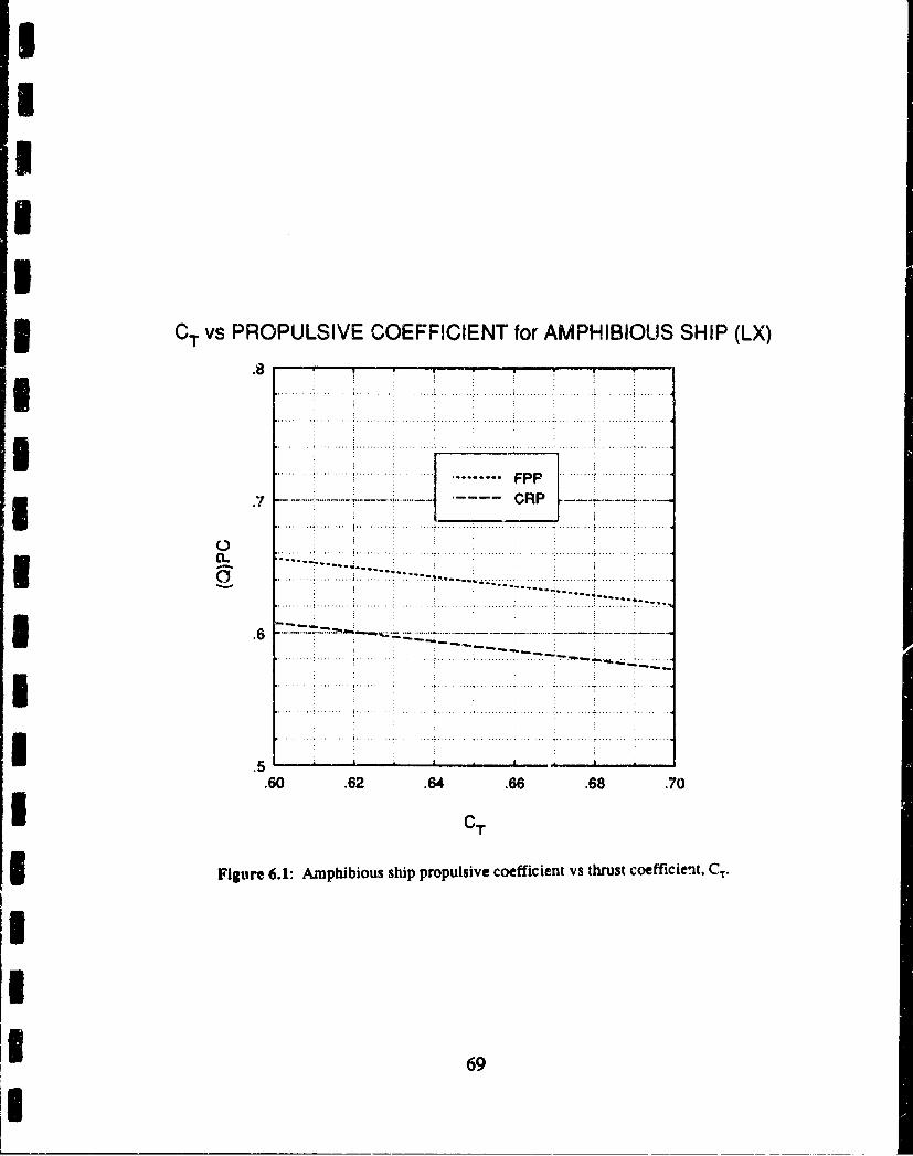
3 0 T vs PROPULSIVE COEFFICIENT for AMPHIBIOUS SHIP (LX)
.. .. .. . .. .. . .. .. .......... .... ... ... ... . . ..
~~.......... .......... ....................
.6 ~ .~ J 7 .
.6 .62 .64 .66 - .68 .70
I CT
I Figure 6.1: Amphibious ship propulsive coefficient vs thrust coefficie-ltCT.
1 69
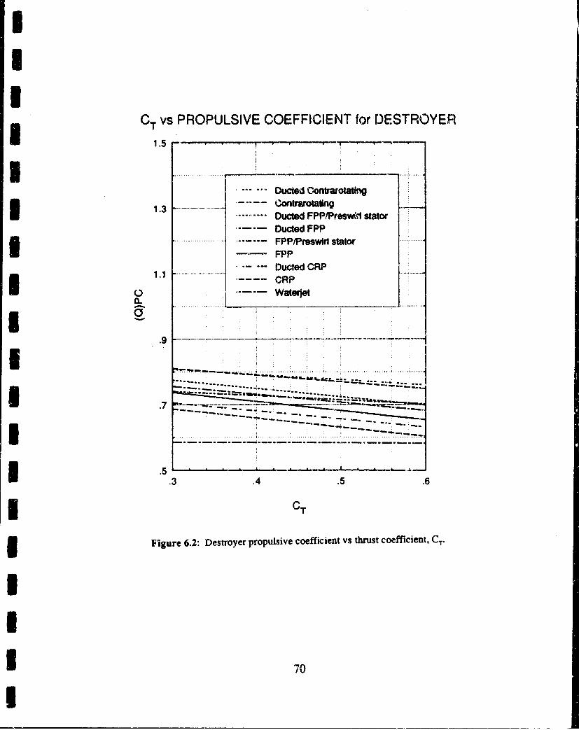
UI
CT vs PROPULSIVE COEFFICIENT for DESTROYER
I _ _ __1.5
*••••••Ducted Contrarota•tgC1ontrarotatingU.1.3.......Ducted FPPfPresw(s1 statorDucted FPP
... . ....... FPP/Preswirt stator
FPP1.1.. -Ducted CRP
1.1 --- CRP
*C 0S~waterjet
.9
.................... ..... a....
!-.5!
I.3 .4 .5 .6
3 CT
Figure 6.2: Destroyer propulsive coefficient vs thrust coefficient, CT.
70
3 screw destroyer, a propeller diameter of 15.2 feet is assumed (justification for this
assumption is provided in Appendix 12).
As mentioned earlier, one of the inputs which "prop-performance" requires
to predict CRP propeller performance is the ship speed when the propellers reach
3 full pitch. This speed is calculated by a separate C function entitled "crpidle".
3 Within "crp-idle" the values for maximum engine rpm and maximum propeller
rpm are used to calculate a gear ratio. The gear ratio is used with idle engine rpm
to calculate the idle propeller rpm. Then, using the ship speed versus advance
3 coefficient correlations, advance coefficient is calculated for the idle propeller rpm
g and, finally, ship speed at that rpm is solved for. At the speed calculated by
"crp-idle", "prop-performance" switches from the constant rpm / varying pitch
I correlation to the constant pitch / varying rpm correlation.
Copies of the "prop-performance" and "crp-idle" functions for the
3 destroyer and amphibious ship are provided in Appendix 13.
I
The Prop-Size Function
3 This function calculates the weight (and internal hull volume when
3 applicable) of the selected propulsor type. If the propulsois selected are
* 71
I

II3 propellers, this function uses the weight (and volume) cor'elations for the various
ducted and non-ducted propellers presented in chapter 4. If waterjets are the
selected propulsors, the weights and volumes of the KaMeWa Model 250 SII
3 discussed in chapter 5 are returned. A copy of the "prop-size" function which is
applicable to either surface ship is provided in Appendix 14.
IIIIII
* 72
IU* Chapter Seven
Choosing the "best" combination of propulsion plant components for a
particular naval ship design is a complex task. This task is further complicated
I because the country's political and economic climate periodically redefines what
I "best" means when applied to design and purchase of a national asset. A computer
program is being developed which will provide cost and performance data for
1 naval ship propulsion plants, to assist the decision-makers in assessing different
component combinations, using whichever criteria they choose.
I Within that computer program, routines characterizing the performance,
3 size and weight impacts of a variety of propulsors were needed. These routines
have been written for up to nine different types of propulsors (eight propeller
1 configurations and one water'et configuration) for three ship types. The
3 correlations for selecting optimum propeller geometry and predicting propeller
3 performance invoked by these routines are the result of propeller computer
modelling carried out using the Propeller Lifting Line (PLL) computer program,
I which was written at MIT for use in preliminary propeller design. PLL-designed
3 propellers were filtered through cavitation criteria developed for each ship type, so
* 73
II
that the propeller efficiencies predicted by these computer routines represent the
performance of only those propellers having reasonable cavitation performance.
I Correlations describing the waterjet configuration were developed from
information supplied by the waterjet manufacturer KaMeWa.
3 To ensure that the propulsor correlations were properly programmed, the
routines were tested for each ship type over a range of displacements and speeds.
They yield realistic predictions over a wide range of ship displacements and
I speeds which are consistent with known propulsor performance for the type of
ship each is associated with.
I
Recommendations for Further WorkIThe ability to model propeller designs and predict performance using PLL
I was invaluable. Without this capability, the collection of data used to characterize
propeller design and performance would have been limited for several of the
propeller types of interest. As stated in chapter two however, PLL was designed
to be a preliminary design tool, and other methods are available to predict more
I accurately the off-design propeller performance in steady and unsteady flow. A
technique was developed to use PLL to predict off-design performance. While the
* 74
I
II
data resulting from applying this technique are consistent with known propeller
performance, the off-design performance information obtained by using PLL
could be further verified by using the steady flow panel methods of the Propeller
3 Steady Flow (PSF) program. Similarly, evaluating the cavitation performance of
PLL designs using Burrill's criterion could be further validated by using the
unsteady flow panel methods of the Propeller Unsteady Flow (PUF) computer
I program. While PSF and PUF programs do not exist for all propeller
configurations included in this project, those that do exist could be used to validate
the PLL methods described herein.
3 Prior to this project, PLL had not been used to compare such a wide range
of potential propeller configurations for the same ship application. Additionally,
I corroboration of PLL output with the Burrill cavitation criterion had not been
done. As a result, two suggested changes to the PLL user interface arose during
this effort:
an item should be added to PLL's main menu which allows the user tochange the hub centerline depth. Presently, if the same propeller is beingstudied for use on two ships of different displacement (affecting hubcenterline depth), PLL must be exited and then reentered using a new inputfile.
since the Burrill cavitation criterion is widely accepted, thenon.-dimensional thrust factor, -;c, used by Burrill could be calculated andprovided in the PLL output summary.
75
I
* References
(1) Rains, Dean A. and John A. Johnson. "Cruiser, Destroyer, Frigate Technology
I Assessments", American Society of Naval Engineers Symposium, 1990, p. 142.
I (2) Ibid.
U (3) Kerwin, Justin E. and David P. Keenan. "Computational Aspects of
Propulsor Design", Presented at Marine Computers '91, The 2nd Symposium on
Computer Applications in the Marine Industry, SNAME New England Section,
Boston, MA, September 1991.I(4) Schlappi, Herman C. "An Innovative Energy Saving Propulsion System for
Navy Ships", Naval Engineer's Journal, April 1982.I(5) Kerwin and Keenan. "Computational Aspects of Propulsor Design".I(6) Coney, W. B. A Method for the Design of a Class of Optimum Marine
Propulsors. PhD thesis, Department of Ocean Engineering, Massachusetts
I Institute of Technology, August 1989.
II* 76
I
II
(7) Hsin, C. - Y. Efficient Computational Methods for Muki-Component Lifting
Line Calculations. Master's thesis, Department of Ocean Engineering,
Massachusetts Institute of Technology, 1986.I(8) Kerwin, J. E., W. B. Coney and C. - Y. Hsin. "Optimum Circulation
I Distributions for Single and Multi-component Propulsors", Twenty-first American
Towing Tank Conference, 1986, pp. 53-62.
3 (9) Kerwin, J. E., W. B. Coney and C. - Y. Hsin, "Hydrodynamic Aspects of
Propeller/Stator Design", Proceedings of the Society of Naval Architects and
Marine Engineers Propellers '88 Symposium, Virginia Beach, VA, September
I 1988.
(10) Coney, William B. MIT-PLL User's Manual. Department of Ocean
I Enghieering, Massachusetts Institute of Technology, November 1988.
I (11) Ibid.
U (12) Coney. A Method for the Design of a Class of Optimum Marine Propulsors.
I(13) Comstock, J. P., editor. Principles of Naval Architecture, Society of Naval
I Architects and Marine Engineers, 1967, p. 408.
II 77
I
II
(14) Harvaid, SV. AA. Resistance and Propulsion of Ships John Wiley and Sons,
New York, 1983, P. 218.I(15) Kerwin and Keenan. "Computational Aspects of Propulsor Design".
(16) Wind, Jaap. "Hub Size Selection Criteria for Controllable Reversible Pitch
Propellers as a Means to Ensure System Integrity", Naval Engineer's Journal,
I December 1978.
(17) Advanced Ship Synthesis Evaluation Tool (ASSET) User's Manual, David
'Taylor Naval Ship Research and Development Center, Volume 2C, Weight
* Module.
(18) Svensson, Rolf. "The KaMeWa Water-jet Propulsion System", Maritime
Defence, December 1987, pp. 427-436.
(19) Svensson, Rolf. "Water Jet Propulsion of Large Naval Craft", American
Society of Naval Engineers Symposium, 1990, pp. 24-43.I(20) Ibid.
(21) Svensson. "The KaMeWa Water-jet Propulsion System".
(22) Ibid.
78
!I
* Appendix One
PLL Wake Files
The following files were created to describe the wake velocity fields at the
propeller inflow for a destroyer, an amphibious ship and a submarine. The
I destroyer and amphibious ship files were created from wake velocity data
Sprovided by David Taylor Model Basin for DDG-51 and LSD-49, respectively.
The wake velocity data used to create the PLL submarine wake file was read from
Figure A-1, which was taken from course notes for the Submarine Design Course
-- taught during Professional Summer at MIT by Captain Hmiry Jackson, USN(Ret).
i Destroyer Wake File
PROPELLER LIFTING LINE RUN: DDG 10 FEB 1992********************* WAKE INPUT FILE **************
NUMBER OF RADII FOR INPUTS: 6NUMBER OF HARMONIC COEFFICIENTS (axial, radial, tangential): 7 3 2NONDIMENSIONAL RADII FOR INPUTS:0.4000 0.5000 0.6000 0.7000 0.8000 0.9000AXIAL VELOCITY COSINE HARMONIC COEFFICIENTS:0.9917 O.9909 0.9810 0.9721 0.9665 0.9657-0.0373 -0.0222 -0.0169 -0.0151 -0.0140 -0.0152-0.0212 -00135 -0.0082 -0.0050 -0.0024 -0.0009-0.0081 -C.0051 -0.0020 0.0004 0.0029 0.00530.0015 00005 0.0014 0.0030 0.0039 0.00640.0044 C.0030 0.0034 0.0039 0.0033 0.00570.0051 0.0036 0.0036 0.0042 0.0036 0.0053AXIAL VELOCITY SINE HARMONIC COEFFICIENTS:0.0000 0.0000 0.0000 0.0000 0.0000 0.0000
79
II
-0.0257 -0.0155 -0.0142 -0.0168 -0.0192 -0.0198-0.0251 -0.0175 -0.0140 -0.0137 -0.0148 -0.0156-0.024 -0.0159 -0.0106 -0.0089 -0.0089 -0.0087-0.0169 -0.0108 -0.0065 -0.0051 -0.0032 -0.0026-0.0100 -0.0045 -0.0016 -0.0020 -0.0010 -0.0011-0.0016 -0,0012 0.0018 0.0006 -0.G003 0.0000
RADIAL VELOCITY COSINE HARMONIC COEFFICIENTS:0.0036 0.0110 0.0088 0.0071 0.0040 -0.00290.0079 0.0066 0.0058 0.0053 0.0048 0.00270.0036 0.0054 0.0071 0.0061 0.0054 0.0050RADIAL VELOCITY SINE HARMONIC COEFFICIENTS:0.0000 0.0000 0.0000 0.0000 0.0000 0.00000.0057 0.0036 0.0013 0.0001 0.0048 -0.00460.0092 0.0091 0.0085 0.0082 0.0070 0.0058TANGENTIL VELOCITY COSINE HARMONIC COEFFICIENTS:-0.0066 0.0128 0.0129 -0.0019 -.0.0018 0.0063-0.0077 -0.0027 -0.0024 0.0034 0.0053 0.0071TANGENTIAL VELOCITY SINE HARMONIC COEFFICIENTS:0.0000. 0.0000 0.0000 0.0000 0.0000 0.00000.0104 -0.0007 -0.0008 0.0027 0.0022 -0.0033I
I Amphibious Ship Wake File
PROPELLER LIFTING LINE RUN: LSD 10 FEB 1992S***A***************** WAKE INPUT FILE ***** * **NUMBER OF RADII FOR INTUTS: 6NUMBER OF HARMONIC COEFFICIENTS (axial, radial, tangential): 7 0 7NONDIMENSIONAL RADII FOR INPUTS:0.4000 0.5000 0.6000 0.7000 0,8000 0.900(0AXIAL VELOCITY COSINE HARMONIC COEFFICIENTS:1.0056 0.9906 0.9694 0.9595 0.9536 0.9428-.0.0113 .0.0215 -0.0366 -0.0479 .0.0578 ..0.0658
0.0178 0.0102 0.0003 -0.0066 -0.0126 -0.01720.0128 0.0107 0.0062 0.0048 0.0026 0.0020-0.0007 0.0030 0.0064 0.0088 0 0101 0.0107.0.0078 0.0000 0.0070 0.0093 0.0091 0.0100-0.0057 -0.0005 0.0062 0.0061 0.0048 0.0045AXIAL VELOCITY SINE HARMONIC COEFFICIENTS:0.0000 0.0000 0.0000 0.0000 0.0000 0.OCO00.0470 0.0379 0.0240 0.0257 0.0324 0.0358
* 80
I
0.0104 0.0119 0,0153 0.0189 0.0213 0.0238-0.0122 -0.0039 0.0068 0.0111 0.0126 0.0126-0.0189 -0.0140 -0.0038 0.0001 0.0016 0.0037-0.0125 -0.0117 -0.9099 -0.0073 -0.0051 -0.0028-0.0049 -0.0090 -0.0114 -0.0119 -0.0088 -0.0058TANGENTIAL VELOCITY COSINE HARMONIC COEFFICIENTS:0.0365 0.0191 0.0025 0.0085 0.0276 0.02990.0237 CG0029 0.0038 0.0010 -0.0032 -0.00550.004.6 0.0010 -0.0022 -0.0020 -0.0018 -0.00120.0097 0.0050 0.0034 0.0010 0.0013 0.00115 0.0076 0.0075 0.0068 0.0041 0.0014 0.00010.0049 0.0059 0.0072 0.0065 0.0036 0.00150.0016 0.0048 0.0094 0.0071 0.0041 0.0020TANGENTIAL VELOCITY SINE HARMONIC COEFFICIENTS:0.0000 0.0000 0.0000 0.0000 0.0000 0.0000
0.0037 0.0008 -0.0054 -0.0075 -0.0077 -0.00960.0095 0.0059 0.0027 0.0012 0.0004 -0.00050.0068 0.0063 0.0066 0.0060 0.0041 0.00300.0008 0.0031 0.0061 0.0066 0.0037 0.0020-0.0024 0.0006 0.0036 0.0044 0.0018 0.0015-0.0002 0.0009 0.0020 0.0018 0.0014 0.0011ISubmarine Wake File
PROPELLER LIFTING LINE RUN: SUBMARINE********************** WAKE INPUT FILE *********************NUMBER OF RADII FOR INPUTS: 9NUMBER OF HARMONIC COEFFICIENTS (axial, radial, tangential): 1 00NONDIMENSIONAL RADII FOR INPUTS:0.2000 0.3000 0.4000 0.5000 0.6000 0 7000 0.8000 0.9000 1.0000AXIAL COSINE HARMONIC COEFFICIENTS:0.4600 0.4900 0.5100 0.5350 0.5800 0.6500 0.69,00 0.7400 0.7900AXIAL SINE COEFFICIENTS:
S0. 0. 0. 0. 0. 0. 0.0. 0.
*81I
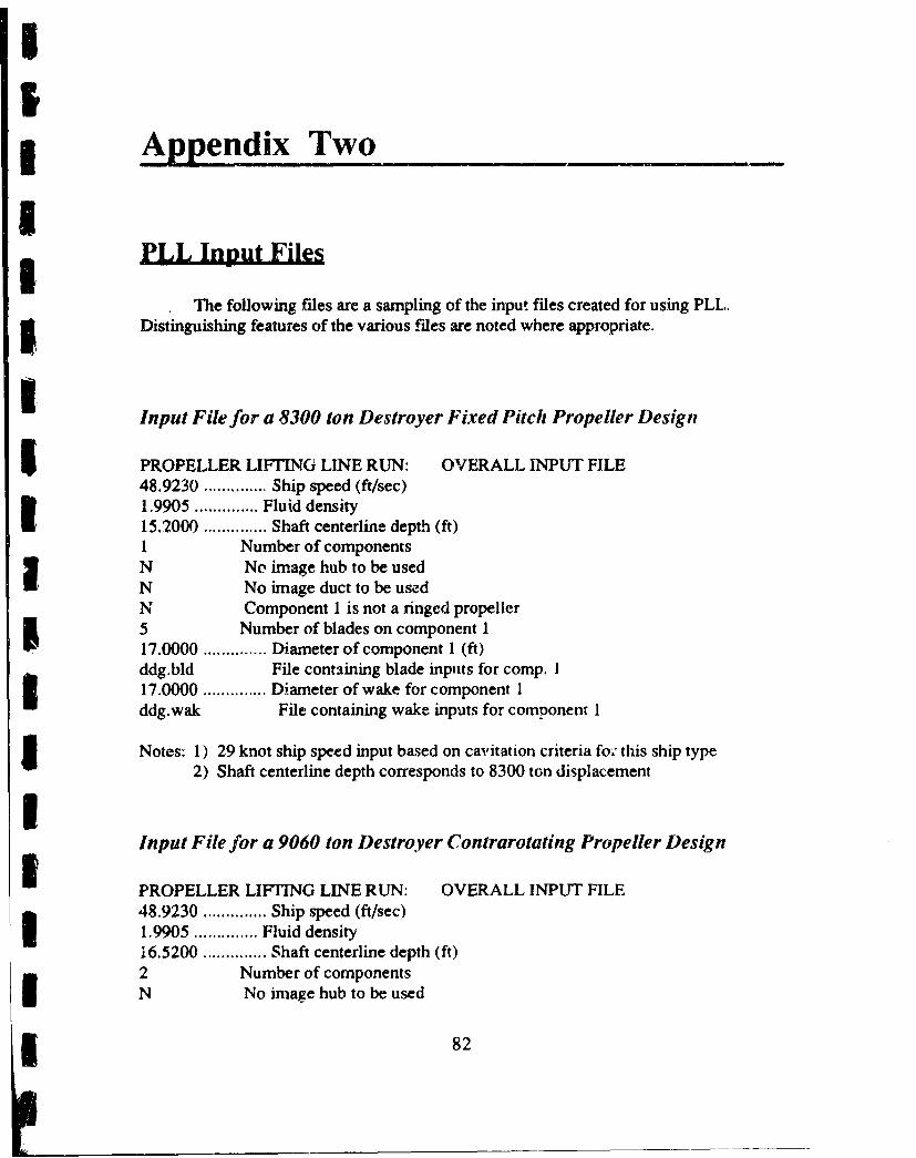
II* Appendix Two
IELL Input Files
The following files are a sampling of the input files created for using PLL.S Distinguishing features of the various files are noted where appropriate.
Input File for a 8300 ton Destroyer Fixed Pitch Propeller Design
5 PROPELLER LIFTING LINE RUN: OVERALL INPUT FILE48.9230 ............. Ship speed (ft/sec)1.9905 .............. Fluid density15.2000 .............. Shaft centerline depth (ft)1 Number of componentsN No image hub to be usedN No image duct to be usedN Component 1 is not a ringed propeller5 Number of blades on component 117.0000 .............. Diameter of component I (ft)ddg.bld File containing blade inputs for comp. I17.0000.........Diameter of wake for component Iddg.wak File containing wake inputs for component I
Notes: 1) 29 knot ship speed input based on cavitation criteria fo; this ship type2) Shaft centerline depth corresponds to 8300 ton displacement
Input File for a 9060 ton Destroyer Contrarotating Propeller Design
PROPELLER LIFTING LINE RUN: OVERALL INPUT FILE48.9230 .............. Ship speed (ft/sec)1.9905 .............. Fluid density16.5200 .............. Shaft centerline depth (ft)2 Number of componentsN No image hub to be used
* 82
SI
N No image duct to be usedN Component 1 is not a ringed propeller2.0000 .............. Axial location of component 1 (ft)5 Number of blades on component 1
17.000...........Diaete o component I ft)
Jdg.bld File containing blade inputs for comp. o17.0000 .............. Diameter of wake for component Iddg.wak File containing wake inputs for component 1N Component 2 is niot a ringed propeller-2.0000 .............. Axial location of component 2 (ft)5 Nuraber of blades on component 217.0000 ....... Diameter of component 2 (ft)ddg.bld File containing blade inputs for comp. 217.0000 .............. Diameter of wake for component 2ddg.wak File containing wake inputs for component 2
5 Notes: 1) Contrarotating design specified through use of two components2) Shaft centerline depth corresponds to 9060 ton destroyerI
Input File for 8500 ton Destroyer Ducted Propeller/Pre-swirl VaneCombination
PROPELLER LIFTING LINE RUN: OVERALL INPUT FILE48.9230 .............. Ship speed (ft/sec)1.9905 ....... Fluid density17,2500 .. ... .Shaft centerline depth (ft)2 Number of componentsN No image hub to be usedY Image duct to be used0.5000 ........... (Duct chord length)/(Component #1 diameter)0.0085 .............. Drag coefficient for the duct0.0 750 .............. (Duct thickness)/(Component #1 diameter)17.7500 .............. Duct diameter (ft)0 ............... Axial location of duct mid-chord (ft)2.0000 .............. Axial location of component I (ft)5 Number of blades on component 117.0000 .............. Diameter of component I (ft)ddg.bld File containing blade inputs for comp. 117.0000 .............. Diameter of wake for component 1
S3 83
I
II
ddg.wak File containing wake inputs for component INu robdocn-2.0000.........Axial location of component 2 (ft)
5 Number of blades on component 2
17.0000 .............. Diameter of component 2 (ft)ddg.bld File containing blade inputs for comp. 217.0000 .............. Diameter of wake for component 2gddg.wak File containing wake inputs for component 2
Notes: 1) Dimensions of the duct defined in this input file2) Propeller/pre-swirl combination specified similarly to contrarotating propeller;when component rpin i3 input to be zero, PLL assumes that the component is astator.
SI Input files for several displacements of each ship type were creased, and diffirencesbetween those files and the sample included here involved:p • specifying the correct cavitation design speed for the ship type,
* adjusting the shaft centerline depth for the displacement,
S•choosing the correct number of propeller components,
. choosing the correct piopeller diameter for the ship type, and
I scifying duct dimensions for ducted designs.
II
I
5I3 Appendix Three
ILDestrgyer Propeller Design Performance
Figures A3. 1-A3.8 depict destroyer propellei open water efficiency versus
thrust coefficient for the various propeller types considered during this project.
I All data in these figures represent propellers which satisfied the cavitation
5 standard developed for the destroyer design (<20.7% back cavitation when
evaluated using Burrill criterion at 29 knot ship speed). The thrust coefficients in
these figures represent thrust at 29 knots.
8IIi
1 8
II
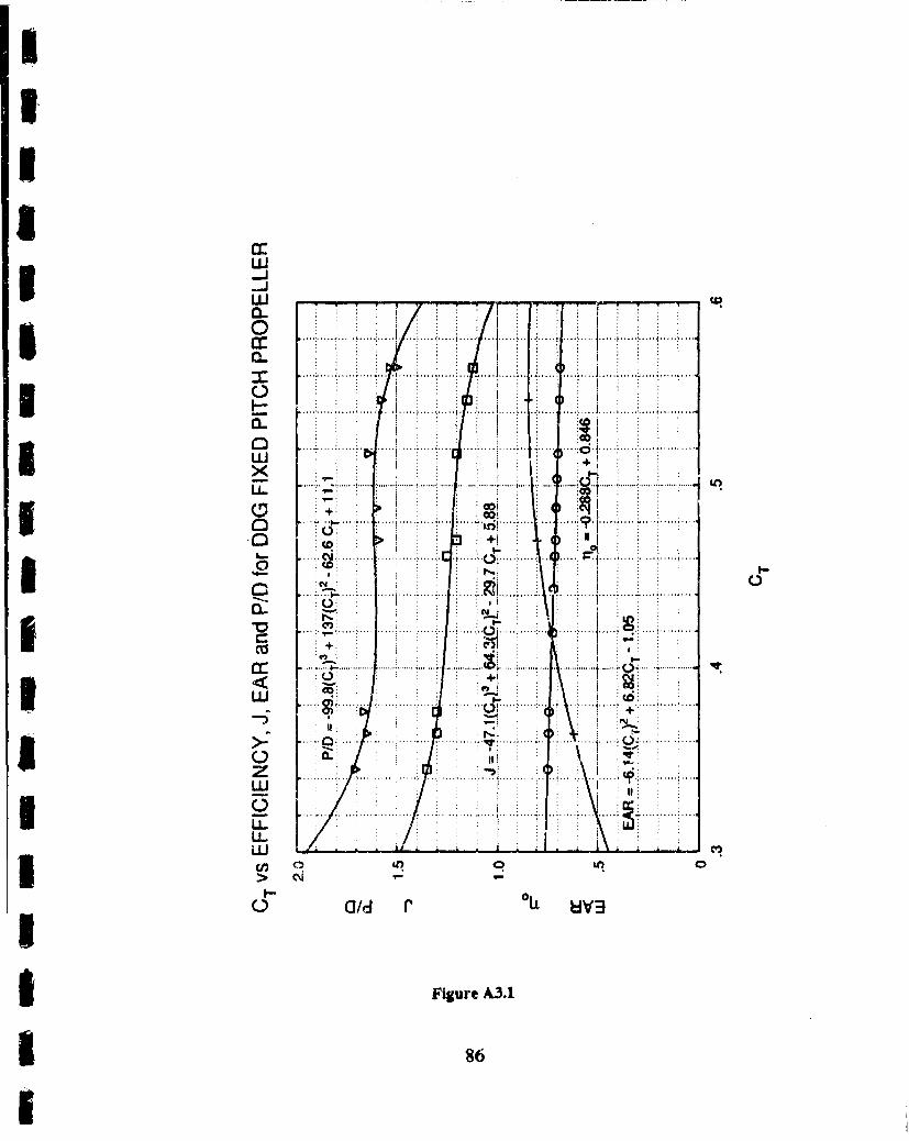
IL
I -j-JwL (
F--
.~ ....... :... ...
++
...........
.. . . .. . . .. I
o000
...........
I .. ....7 .... ..7 .+ .
* Icc 4- .
- +>
w a/ rOL 0
I Figure AM
86
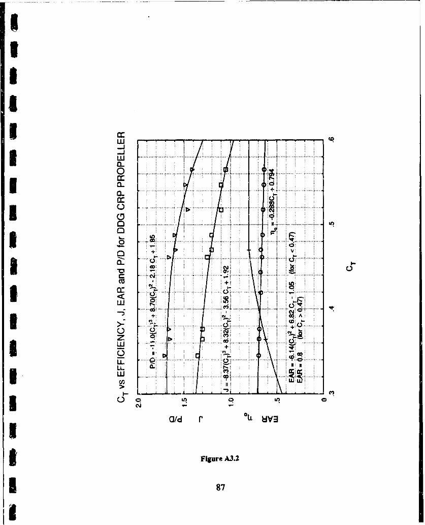
w -9-r-.,--7
... .... I . ..I CL..~.. ... .... .. ....... .. ...
CC
C.)
Iw.. ... .ca~
CC .......0
w ...... .4 .....
IL ....LL 0 f
cn J
Old r HL V3
ft Figure A.3.2
* 87
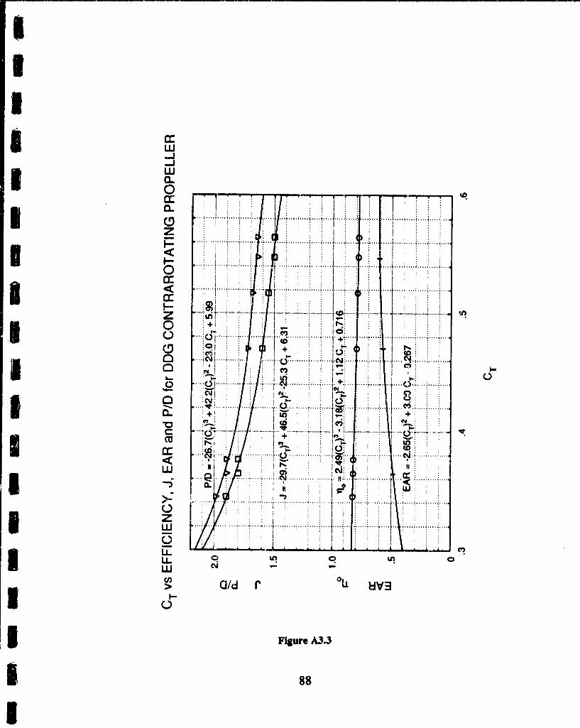
a w:-LJ
w
............ "j. ............
z Ati
ho. C4- : :
C cmJ ... ... ....
cr. ... 1
.. .. .. .. ..... : .. .. ....
IL,
w CJI -~ S/1
>1 .1Tr LL WV
FigurA
0 88
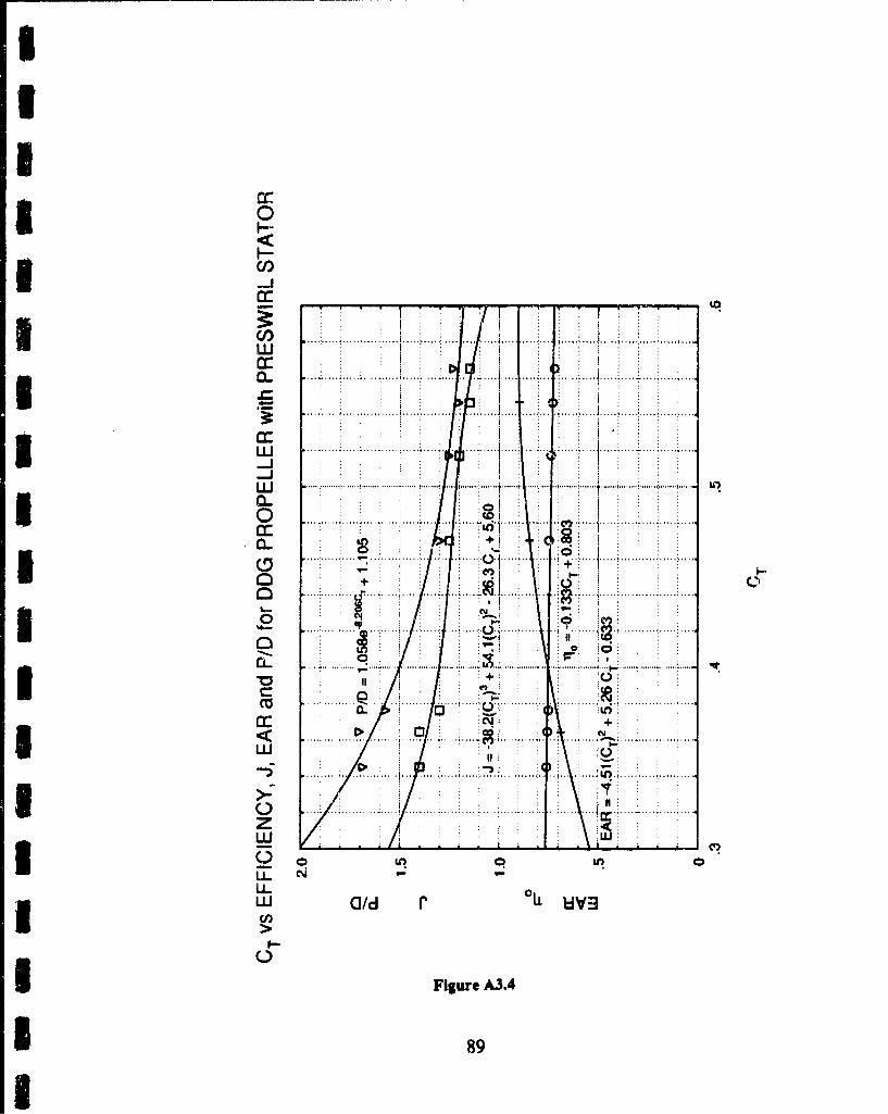
1 0U)
H7U) ...... ......... .. .. .......-Ja - .. ..._ ... .. ..._. ....._ _. .. .._. ...
C,) ....... .....I6 ... ..
0~ ...do....C:(3
01.1
0; ......
w 0 L
£ 0 Figure A3.4
* 89
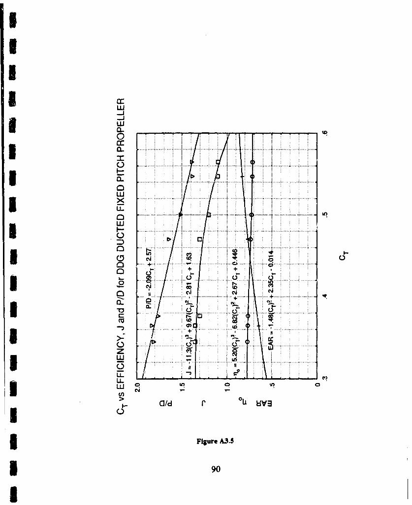
IL
ICLE.......w. .... ..... .....
.. ............ .... .....
-J
I. .......
I 0 ~ ..........
... ..... . .
* 0ý4004
.. ...... ~... . ......
w o 0
.. .... ..... .. ...CCal
3n 0
3 Figure A3.5
5 90
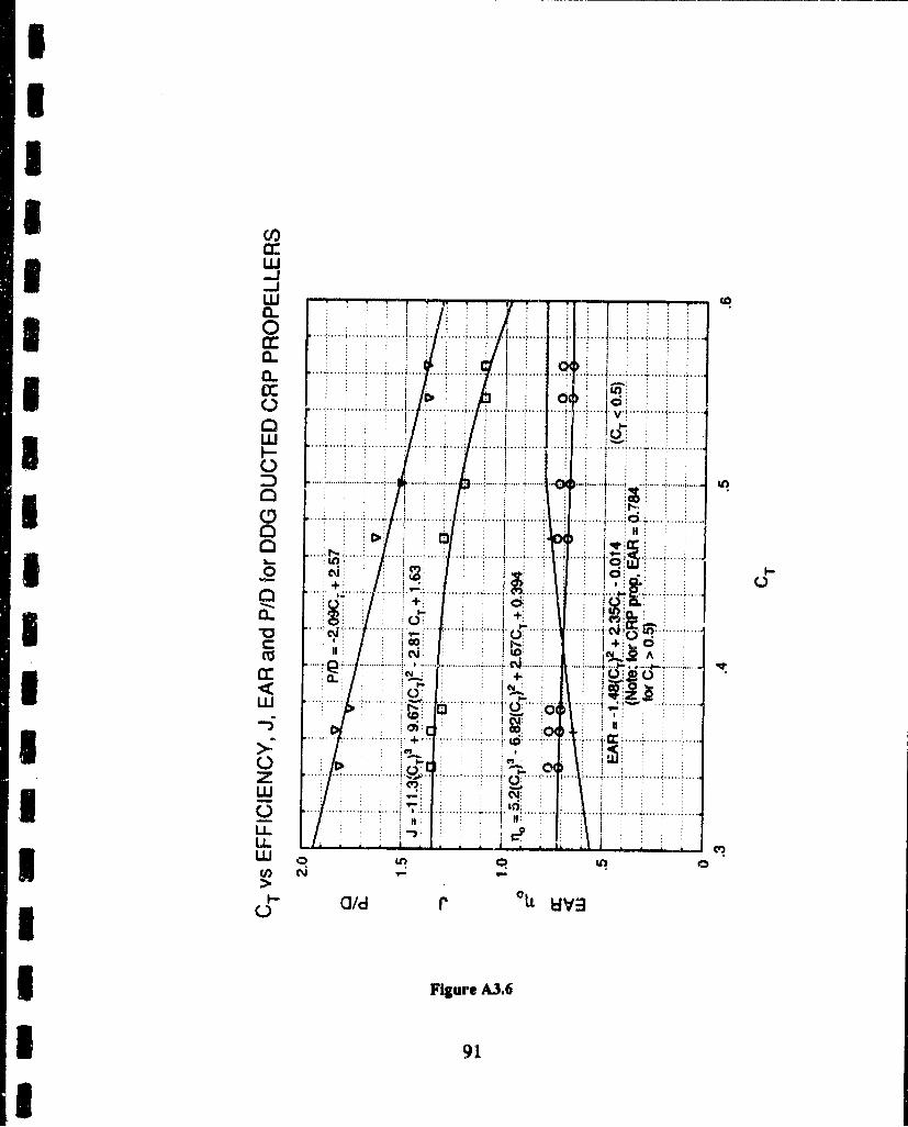
-LJ
a.
*_ 0
L ........................
*. ... .... . .....0 eq:
+n .... .7. .... . .. ... ...
.4: 1+
1J .... . -.. +.. ......... . F... ..
... .. ..
LLJ 1 F
1 /Od r ULL Wva
I Figure A3.6
1 91
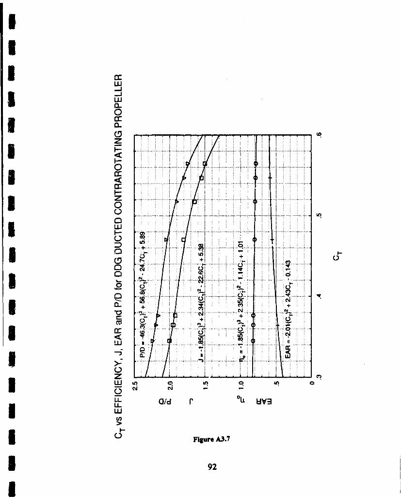
IcIL
0~
.I . . . .. ... ...
cc.. .. ... ...... .. .... .....Ic
0
An ~ ~ ... ... . . .....
co 0
(C;4
C) C
O/d; r *. y
U--3 4: .C;. * *1LU
wFigure A
92I
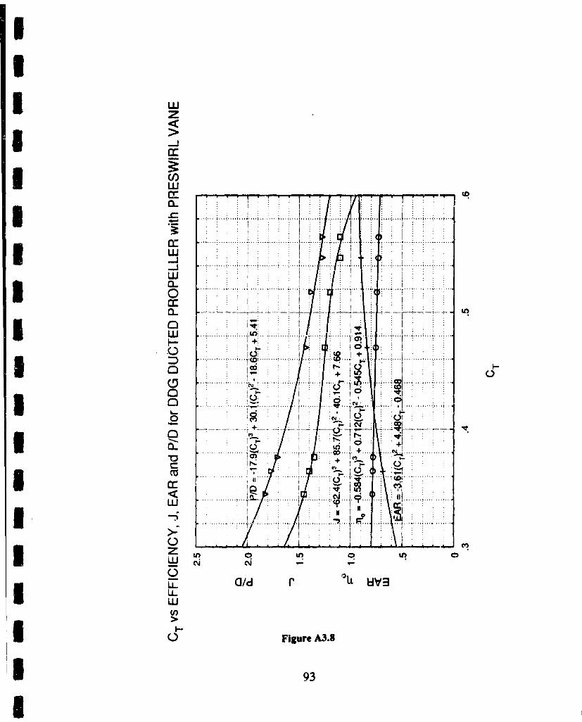
ULz
0aw. >.....................V
w 1U
I0 - I. P i
+
1~ '3
w N N +DL P! .......
U-OI+...... .... . ..IC .. Figure.....
1l .. .....9 3. ...- ............I.. .... .... .... .... c .. ....... ...
I
* Appendix Four
5AmpUhibious Ship Propeller Design Performance
Figures A4.1-A4.2 depict amphibious ship propeller open water efficiency
versus thrust coefficient for the propeller types considered during this project. All
I data in these figures represent propellers which satisfied the cavitation standard
5 developed for the amphibious ship design (<14.5% back cavitation when
evaluated using Burrill criterion at 23.25 knot ship speed). The thrust coefficients
in these figures represent thrust at 23.25 knots.
IIIIII
1 94
Ii
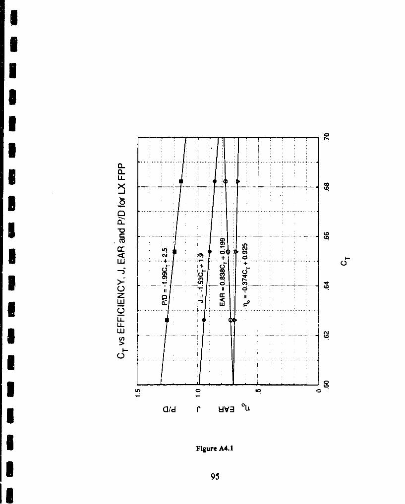
......I. .. ... ..... .................
0~ ...... .... .... .. ....... ...... .........
3o p
00
LU,
....... ..... ..... .... ...
w . + 0
>7
U-
LL
Sn q U,
3Old r Uva L
Figure A4.1
* 95
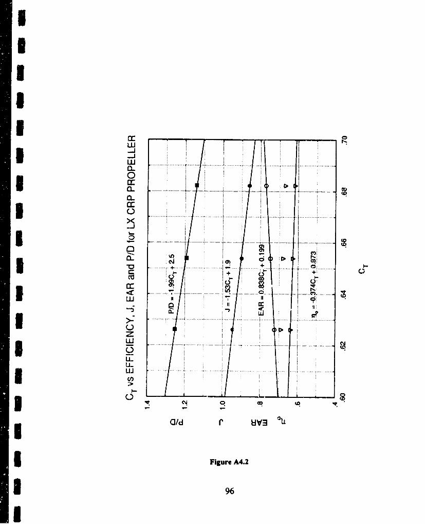
-LJ
LIJ ~ ~~..... ...... .... ........ .................CL
ool
1. ..... .. .. .. .. .. .. .. ... .. ....
I - - t ¶......o. .... ........ ......................... ... ........... C. ... .......... .......
CL)
.. ....... .. ... .. .. .. ..0.. ...CC+4-:-
......~C ........ v .. - .....
... .. .. ... .... . ......1 - I.-
a. IIJ
U-
U-U - ... ........ ..... ... ............ .........
0/Od r HV3
I Figure A4.2
* 96
Appendix Five __
Submarine Propeller Design Perfoma c
Figure A5. 1 depicts submarine contrarotating propeller open watel'
efficieiacy versus thrust coefficient. All data in this figure represent propellers
which satisfied the cavitation stndard developed for the submarine design (0%
back cavitation when evaluated using Burrill criterion at 27 knot ship speed). The
thrust coefficients in these figures represent thrust at 27 knots.
97
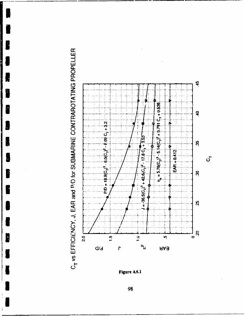
-LJ1 -LJ
0~
..... . ...... ........
cc .............. .... .. ... . ..
; : I : m 4.. .I
...... .. .... U9
5 .... ...... ............... '... ..........,Ci
4 1 -1 ...-. ... . ..... ....
0 4-
.. . ..... . ...
I VVL U .. ... . . . . .. . . . ..... .. U.. t- ,. .li . .
... .....
o...............
U-U
Figure AS. 1
* 98
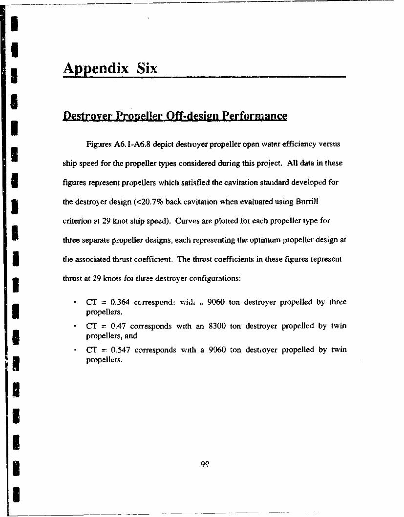
I
* ~Appendix SixI
Destroyer Propeller Off-design PerformanceIFigures A6. 1-A6.8 depict destroyer propeller open water efficiency versus
ship speed for the propeller types considered during this project. All data in these
3 figures represent propellers which satisfied the cavitation standard developed for
5 the destroyer design (<20.7% back cavitation when evaluated using Burrill
criterion at 29 knot ship speed). Curves are plotted for each propeller type for
I three separate p-ropeller designs, each representing the optimum propeller design at
the associated thrust coefficient. The thrust coefficients in these figures represent
i thrust at 29 knots foi three destroyer configurations:
CT = 0.364 correspond, with i, 9060 ton destroyer propelled by threepropellers,
CT = 0.47 corresponds with an 8300 ton destroyer propelled by twin5 propellers, and
CT =, 0.547 corresponds with a 9960 ton destioyer ptopelled by twin* propellers.
9UI* 99
I
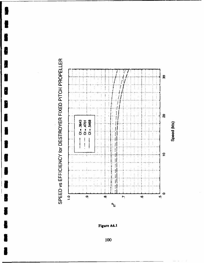
cc
IL ..... .. 7... ....
cc *. I
... .. .. ... ..
......... .. ....
> ................ . . . . . .. . . ..... :........ .............. ......... I.............
LU 0?C 4 l
U?) .iLj
1Figure A6.
* I00
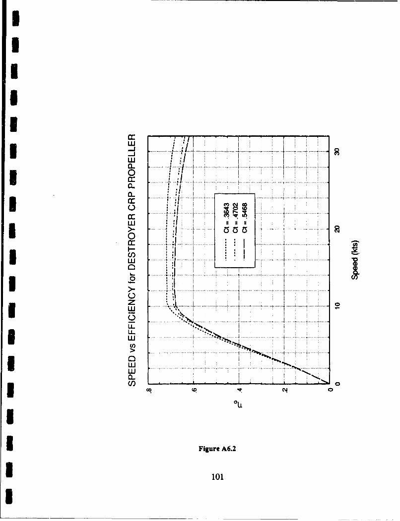
IIII
CCpILLi :i:Ia .......... . • . ....... ......; .......i ...... ......i ......i ......i ...... • .. ..... . ..: ..............
.. . . . . , . . ,.. ....... ;.. . . .. ..... . ..... .. . . .... . .. • . . . . . ... . . .. ... .... . . . . . .
I .......... ~~ ~. ". ':... . .i...... !....... . ...... •...... '. .... .•...... "...... •......
o 6.,o : 'I
.. ........... !. ....... ....... . .1, I I ........ .. .. , ............... ...... ,L 4 . . ' i' 4
4 .,.i Cl
...... •.'! .•... ... .. .. ... ,....•... ... .......
o ' 1 ... ..0.
• -........... '~~..' . . . . .i. . . . . .;...... ;...... •...... ...... ...... ...... ...... i ...... : ............
I .. ....... .. ........ .• .. .. ........ ....... • ... .......... •. . ......... .. .......... ....... ... .... •.......LLI
SI , , , ....... ...... ...... • ..................:• • ...... : ...... t ............. 7 .... .• ...... •.......LL I..........•......... ......... ............... ,...... •...... ....• _.:.........
I _
CLt
I
I Figure A6.2
101
J -"w
...... .. . . ... . . . . ...... : : : T .....
S..... . ,.-.. -.. ,... .. ,. ... •.. .. :. ,, , .,, . , ; .... .... . ..• - .. .. . ... . ... .. ... .. .. . . ......I 4' I : 4:,n i i :
.... :" '" ' " ': " 'V " '" 'f ".' " !'" ''i" T ".l' ' . ... . .. ..... .... ....": " ' ' ': " !' ......... : " •....
S. .. .. .. .. . . .. .. ........... . I. H ....... ... : .... .......... .. . . . . . . , ........ . . . . . .
I' , ti*19' . * j. . . . . .
S....."! " ' : i ":.... ..... ."i " f' : " : ........ .......".':' 'I '' ' ' .. .... . . . .
z .. . :II ' ' i,F-I
o . . [1
i... .... . ....... ... .... . ...
I , I II
"w- *1I'S• . . . . . . . . . . .............. .... 'T. .. . ... ... ... ...... ........ .............. .. . . . . .
. /...................... - o iil 4i ! 0
• i , In ~:1:II. .w . ... .... ....... . ......... ........ . ...........
*, I IIII. ...... ... .. . .. ........
I 102 li
I
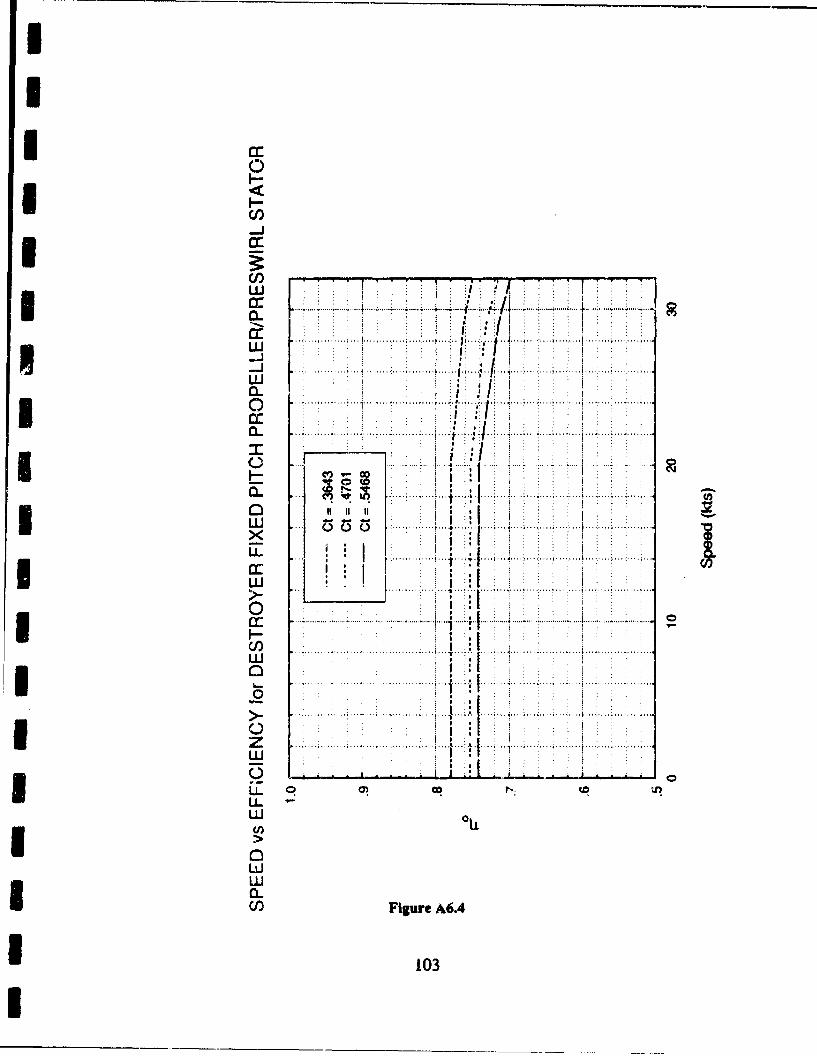
0
U,)-J
pr ........ ...~.
IC.. ...... ..
.. ..... ...... ........o 1.. ....I. ..... .. ......
0V)00I I
UU _ _ _ _ ~.'. .........
I 103.. .......... .........
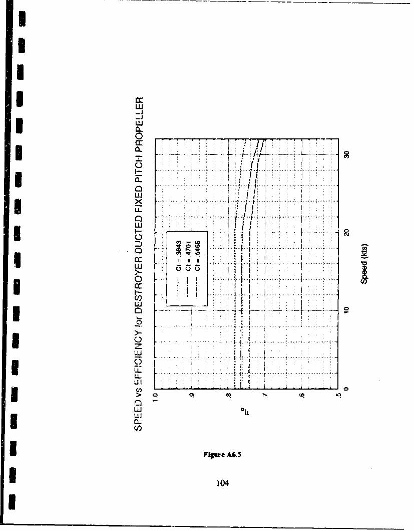
IIII a:
LU-J
a.. ..... . . . .. .. . . . . . ..
" ..... ... . .. .1AS. .... ....... ...• . . ;... .. .. .. ... .• A ." .I • . : . . . .. . ..: .... + . : . . .I... ...
. . . .. . . .. . ... + , .... ............. ... .I ... :.. ... ..... ..... . ' .... ... . - . .....+ .. ........ ......
ILU ! ~ I:: ::
- I X "? ;~~~.. ............. ..."... ... •'.. + . . .... .I'}l ! ! ..• .... . ' " ' • i . ' ...........
.. ..... ... . . : , . . . . . . . . .'
1 ' III : , . ,. . . . I . .
..I.... . ......
w ....... . . .... .. ..I.. ... .. .. .. ... . .. .... .... .... ....
I a: I:I ll
L L' ' .... ... .. .. 'I ... .. .... ; .. •+... .. .. . ., , .. . • . . . . + - , . . . , •
w OIL ' " JuJI Fgr A 6
I 1 . 04
lL. .. . ..I jZ ....... ................... . ''I ........ . . . . . . . ...... I ...... :....
' ' 0
LU o
I Figure A6.5
*n0
l
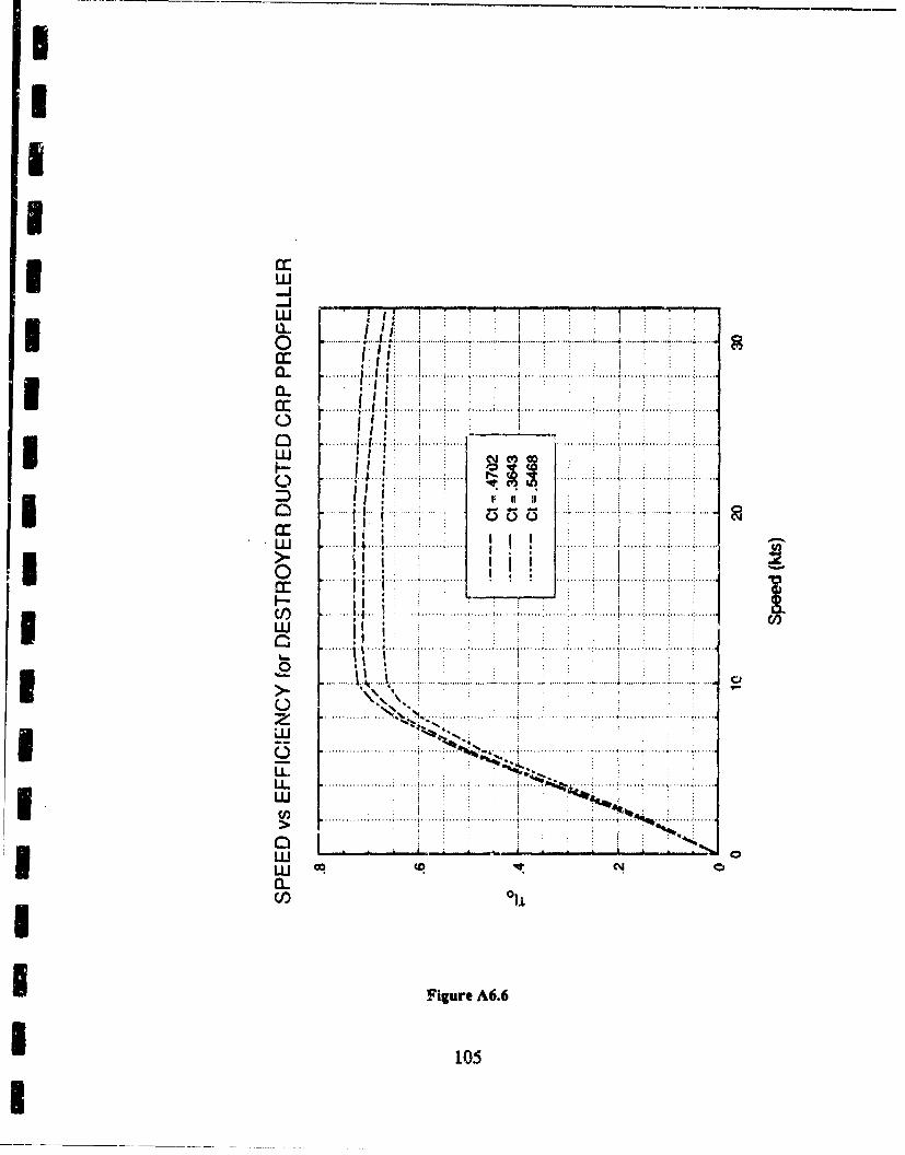
IL
CIL
CL. .. . .L I .[ ..... .i...... ... ..... 1 ... .. . . . . . .i. . . . . .I. . ........ i.......i . ..
i l i t ... ....• s l, , ... ... ... , .. .. ,,, ,, , , i. •. .... • .....t .....• ........ ........ ...LU
I- ... .. I ! : ..... ..... .... ..: .. .i .. ..! .. ... ....• .. .., .. ..Ia
.... ...I ,' '/ " ... .:... .. ... .! • • • I... ...... ....... •.... . ............... . .
|m.~~ ~ ~ ~~ ., . . .. .... . .. .. .• .. ....... . . .. .:. . .. : .. . .. ... .. .. .... . ..
.. .. .. .. ..t , ;: .... .... .. .. ..... ... ...... .. .... ..... ...--.. ... .. .. .. .. .... .. .. .. .. .. .. .... .. ... ... .... .. .. ... ... .[ .. ... .I i : .... i ... .. ... .. .. ...i . .... ...... .... ....... :. . ..i .. . .. ... . .. ...
*. ...
L ... .............. .. . %... .. .......... . . . . . ... i . . . . . . . . . ........ .. .. • . . .............
0 .... ...... ..... : ... .. , . .... ..... "• • ; 1...... •......... . . . . . . .•. . . . . . .
010
n li, •. I Ito
O0 °! •~ -. ~LJJ
•- F~ ~iiur A.
O ~ i0 *
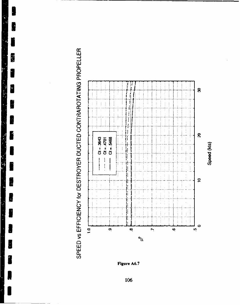
IL
cc
.. .... ..... .... ..... .
cc
........... . .............
.. ..... .. ..... ... .. ...... .
0wLo . (
CL ;I.I
oiur A6.
cc 06
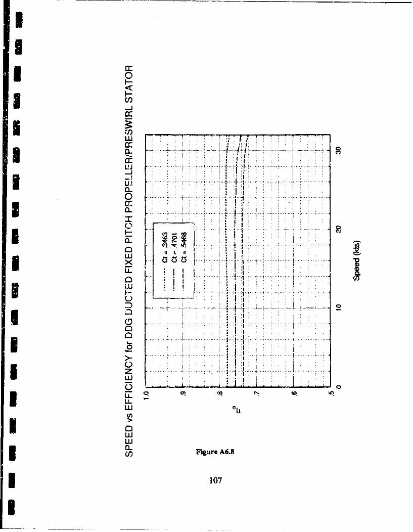
UUUU
* ~cc
W : ... ...... .....
cc
.. .. . ... ... .. ... ..
0
.... ... ..
* ~LiFigur A6.
107..
II* Appendix Seven
IAm• phibious Ship Propeller Off-design Performance
3I Figures A7. 1-A7.8 depict amphibious ship propeller open water efficiency
versus ship speed for the propeller types considered during this project. All data
I in these figures represent propellers which satisfied the cavitation standard
3 developed for the amphibious ship design (<14.5% back cavitation when
evaluated using Burrill criterion at 23.25 knot ship speed). Curves are plotted for
each propeller type for three separate propeller designs, each representing the
I optimum propeller design at the associated thrust coefficient. The thrust
coefficients in these figures represent thrust at 23.25 knots for three amphibious
ship configurations:
CT = 0.626 1 corresponds with a 20,500 ton ship propelled by twin3 propellers,
* CT = 0.6538 corresponds with an 22,700 ton ship propelled by twin3 propellers, and
* CT = 0.6822 corresponds with a 25,000 ton ship propelled by twinpropellers.
3 108
U
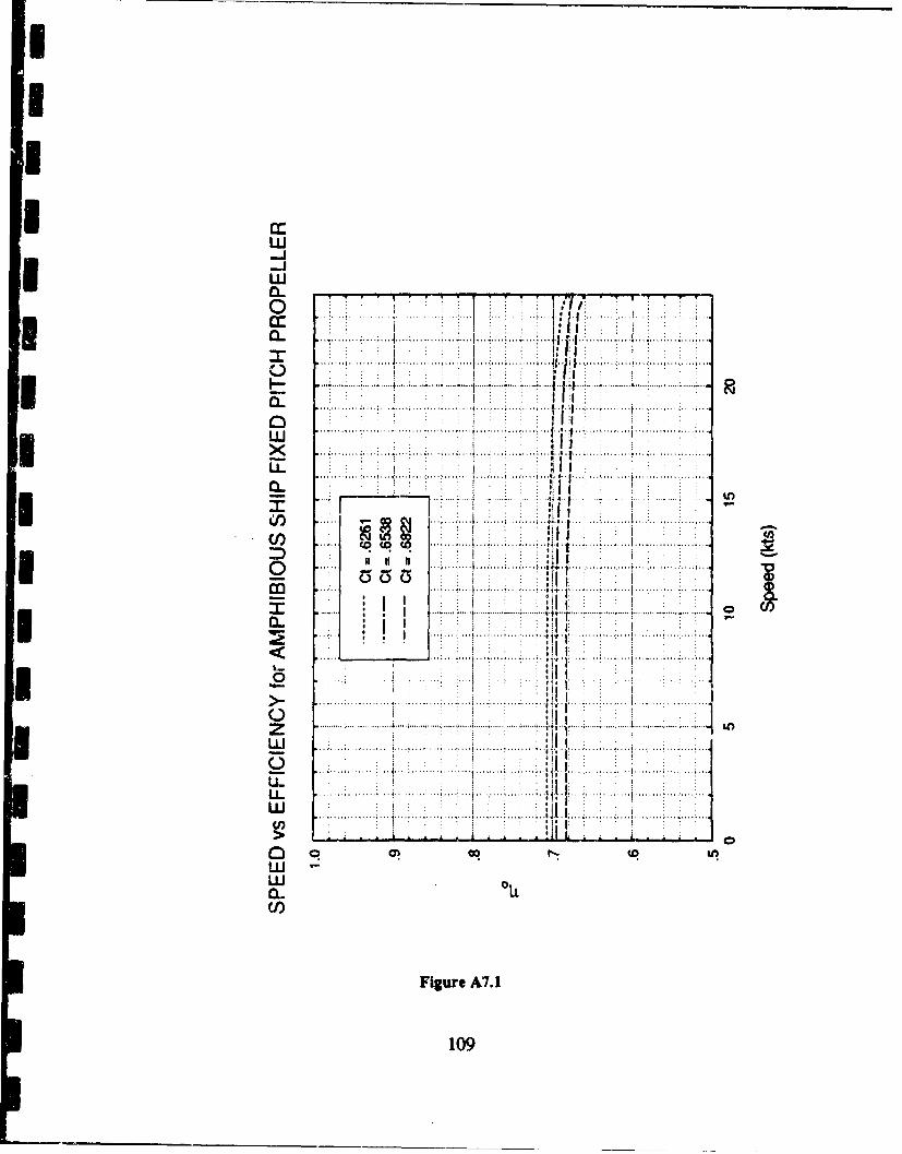
IcILICIa
.. .. ... .
- -...................... .......*... .....
.. .. ... .... ....
iml0 .... ........,
..... ... .. .. ..
..... ..
i .. .. . .. .. .. .. .... .. .
3_ .. .... i ... .... .. .. ... .
........... .... .....>i
LL ...JI
U) I
109
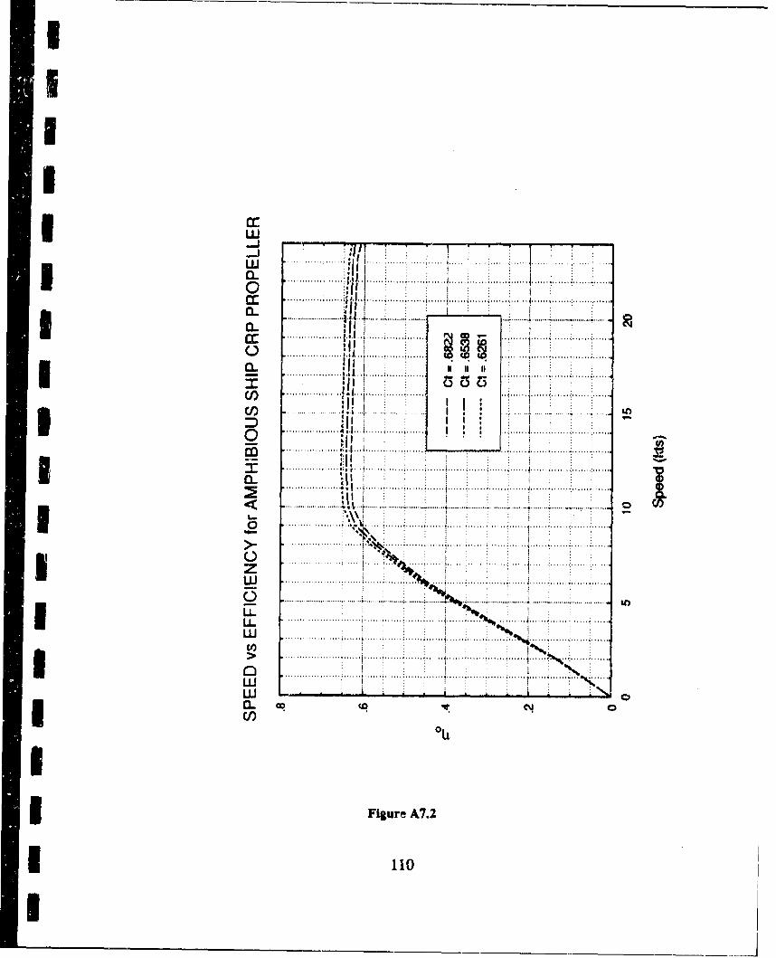
II
II ,,
w.. .. .............
0 . . . ..... .............,I...............c c' .. . . . . . . . . . . . .. . ..
a . ............. ........ ...... ....... ' .. ... ......... ...... •......,.... ....7, 1 .... ...........0..
............. ;...... . . . .. . ... .......... 1i......L...... ,. .
I0..........' ' ...........
cn~:j ... ... ....
0 ...............1 I I.............. ............. ..
..... ..... ........... • • . .........; ...... i .... . ...... !.... .. i ..... ........ •......
Ii If.I i I I II•
......... . .. l l ........ .. ..... ...... .... .............
S.......... ... I ........ . . .......
I -
, z
L , . ... .
> ........ ........ ...,i .l...1 ........ ........ . .. ..... ....... N . ...... .. ..
...........w°l.t....•.......i... ...... .......... ...... i ... I .. ...•...... •.......
w
I II"0: •
1LL
Figure A7.2
110
It, ..............! ... ...• ... ........, • .i ... ...... ... ...
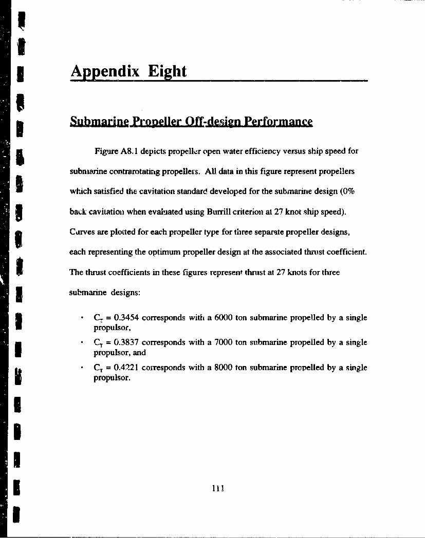
3 Appendix. Eight
Ssign Performance
Figure A8.1 depicts propeller open water efficiency versus ship speed for
subnimrine contrarotatirng propellers. All data in this figure represent propellers
which satisfied the cavitation standard developed for the submarine design (0%
3 back cavitation when evaluated using Burrill criterion at 27 knot ship speed).
3 Cdrves are plotted for each propellcr type for three separate propeller designs,
each representing the optimum propeller design at the associated thrust coefficient.
I; The thrust coefficients in these figures represent thrust at 27 knots for three
I submarine designs:
S C, = 0.3454 corresponds with a 6000 ton submarine propelled by a singleIl propulsor,
- CT = 0.3837 corresponds with a 7000 ton submarine propelled by a singlepropulsor, and
* CT = 0.4221 corresponds with a 8000 ton submarine propelled by a singlepropulsor.
-II
SI11
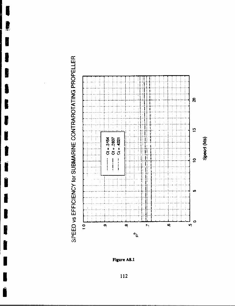
SLILIL
c-J
c c .... ....
.. ....... 4 1 .... ... .....
o'> ......
3 ~ ~ u CcK..Iu;o
>11
!I
Apendix Nine
NControllable Reversible Pitch Propeller PerformanceDuring Constant Speed / VaryinUg Pitch Operation
I Figure A9.1 shows the correlation developed to characterize the
3 perfoanance of CRP propellers during the constant rpm / vaying pitch regime of
operation (typically from 0 to 12 knots). The data points plotted were predicted
using the Wageningen B-series propeller polynomial by matching ship speed vs
thr-ust required with ship speed vs thrust developed by the propeller, while
Sassuming the propeller rpm was constant and the pitch-to-diameter ratio varied.
Data was gathered for different ship configurations, and it was noted that if the
efficiencies were normalized by dividing by the peak efficiency, the same curve
£1 could be used to correlate normalized efficiency to speed for all CRP propellers
analyzed. The correlation is included on Figure A9. 1.
IIII5 113
I
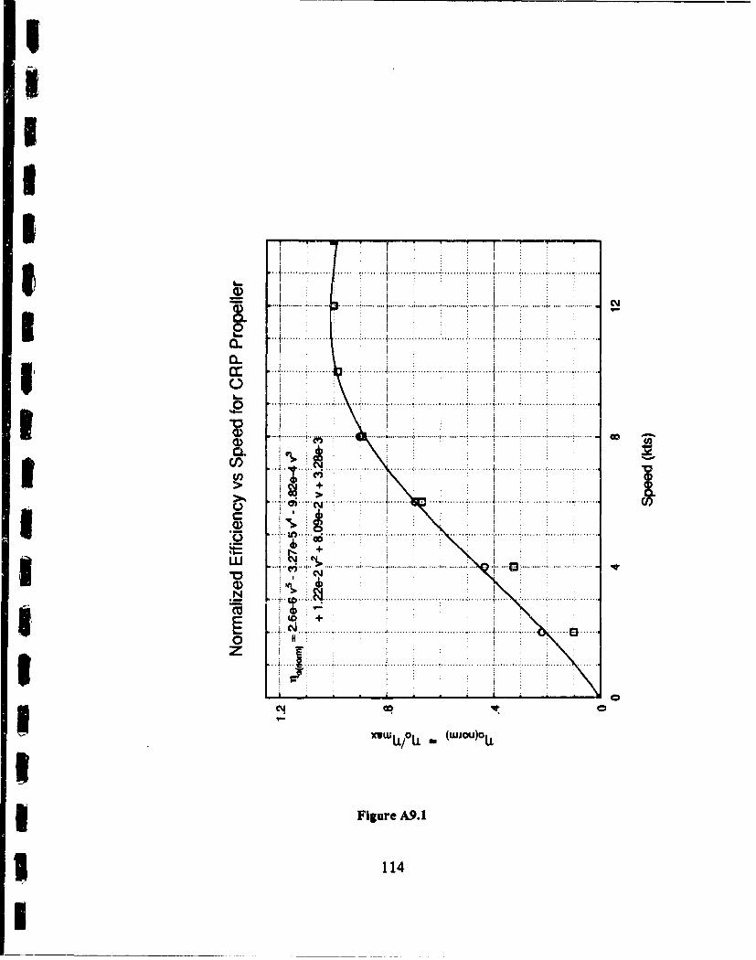
5 ... .... .... .... ...... .... ..... ..... .......... ...
cn cc
.... ... ... ....... ... ... ...
E +C Y .. ..... ... .. ......... 0. . ...
C4I"wWU L .woi)L
Fiur A9.1V114
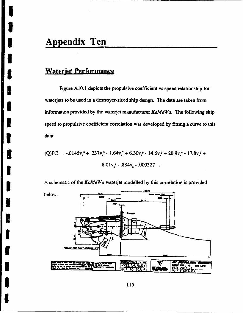
5
5 Appendix TenIS Wateriet Performance
t Figure AlO. 1 depicts the propulsive coefficient vs speed relationship for
watcrjets to be used in a destroyer-sixed ship design. The data are taken from
information provided by the waterjet manufacturer KaMeWa. The following ship
1 speed to propulsive coefficient correlation was developed by fitting a curve to this
3 data:
(Q)PC = -.0145v.9 + .237v,8 -, 1.64v.7 + 6.30v,, - 14.6v., + 20.9v.4 - 17.8v.3 +
8.01v 2 - .884v. -. 000327 .
3 A schematic of the KaMeWa waterdet modelled by this correlation is provided
below. __,---__,-..___
III , 40IJ
S~115
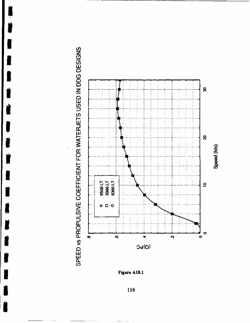
0
....... .... .. .. .....
C/)
C,).. .....H. ... .. ........
wU .. ...I. .... ......... .wL
........ .. ...
.. .....I. ..... .... ..........0 ... .... .... .... . .. ....
Ii-
......L..... ......IU0i
CC)
00
LU
Figure AlO 1
£ 116
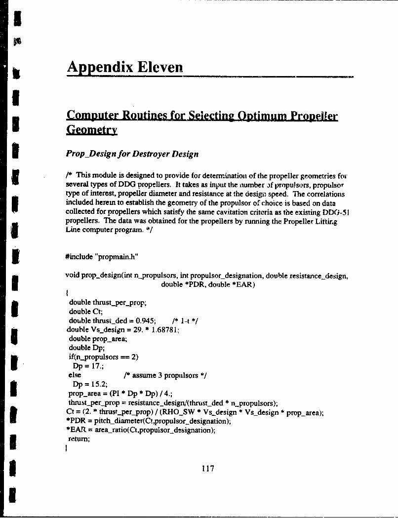
I
Appendix Eleven~
Computer Routines for Selecting Optimum Proeler
Prop-Design for Destroyer Design
/* This module is designed to provide for determination of the propeller geometries foi-several types of DDG propellers. It takes as input the number ,,f propulsors, propulsortype of interest, propeller diameter and resistance at the design• speed. The correlationsincluded herein to establish the geometry of the propulsor of choice is based on datacollected for propellers which satisfy the same cavitation criteria as the existing DDG-51propellers. The data was obtained for the propellers by running the Propeller LiftingLine computer program.
3 #include "propmain.h"
void prop.design(int npropulsors, int propulsor._designation, double resistance_design,3 double *PDR, double *EAR)
double thrustper._prop;double Ct;doible thrust-ded= 0.945; /* 1-t */
i double Vs-design =29. * 1.6878 1;
double prop-area;double Dp;if(npropulsors =- 2)
I Dp = 17.;else /* assume 3 propulsors */
Dp = 15.2;prop-area = (PI * Dp * Dp) / 4.;thrust_perprop = resistance-design/(thrustded * npropulsors);Ct = (2. * thrust_perprop) / (RHOSW * Vsdesign * Vs.design * proparea);*PDR = pitch-diameter(Ct,propulsor-designation);*EAR = arearatio(Ct,propulsor designation);
3 }return;
* 117
I
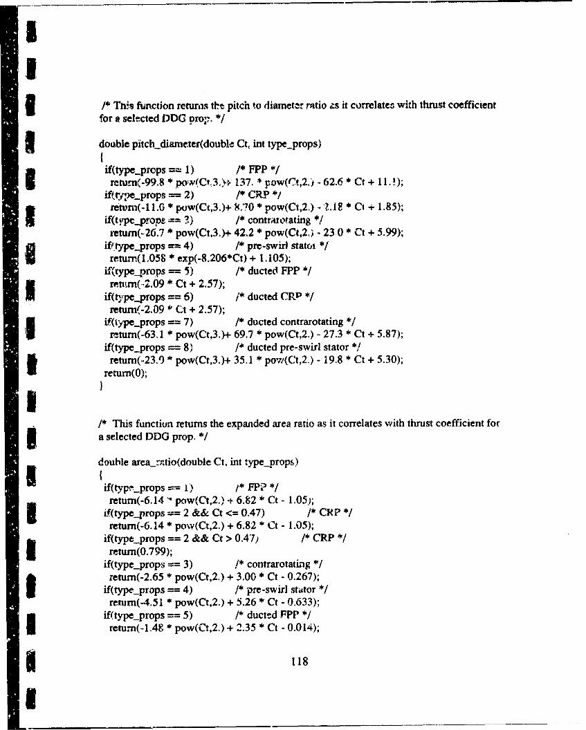
I* Th-9 function returas the. pitch to d~iamneter ratio ts it correlates with thrust coefficientfor a selected DOC prop~. */
double pitch..Aiameter(double Ct, hit type..props)
if(type...props =1) 1* FPP *
return(-99.8 *pow(C#,3.)+ 137. * pow(C7t,2.) -62.6 * Ct + I1A.);-ftpe.props =- 2) /* CR- *
retvrn(-1I1.G pow(Ct,3.)+ 8.70 * pow(Ct,2.) - I. 18 * Ct + 1.8 5);I if~trpe pros 3) * conrrtmtating *retum(.,26.7 *pow(Ct.3.)+ 42.2 * pow(Ct,2.p - 23 0 * Ct + 5.99);
if~rype...props ==4) /* pre-swirl statroiI return(I.058 *exp(-8.206*Ct) + 1. 105);if(type...props ==5) /* ductedi FPP *
rettimr(-2.09 *Ct + 2.57);I ~if(type...props == 6) /* ducted CRP *return(-2.09 *Ct + 2.57);
if(type~props == 7) /* ducted contrarotating/I xetum(-63,1 *pow(Ct,3.)+ 69.7 * pow(Ct,2.) - 27.3 * Ct + 5.87);if (type-props =-- 8) /* ducted pre-swiri stator */3retum(-23.9) pow(Ct,3.)+ 35.1 * po-w-(Ct,2.) - 19.8 * Ct + 5.30);return(O);
1* This functiomn returns the expanded area ratio as it correlates with thrust coefficient for3 a selected DDG prop. */
double area.rmtio(double Ct, int ype.pp)
if(typ(&props 1) * FP? *1retum(-6.14t pnw(Ct,2.) + 6.82 * Ct - 1.05);I if(type..props == 2 && Ct <= 0.47) /* CRP ~return(-6.14 * pow(Ct,2.) + 6.82 * Ct - 1.05);
if(type-props == 2 && Ct > 0.47) /* CRP *I return(0.799);if(type..props == 3) /* contrarotati~ng *
return(-2.65 *pow(Ct,2.) + 3.00 * Ct - 0.267);I if(type-props == 4) /* pre-swirl stastor ~rettrn(-4.51 *pow(Ct,2.) + 5.26 * Ct - 0.633);
if(type-props == 5) /* ducted FPP */
return(-1.48 pow(Ct,2.) + 2.35 * Ct - 0.014);
* 118
I
if(type. props 6 && Ct <= 0.47) P ducted CRP ,retum(-1.48 * pow(Ct,2.) + 2.35 * Ct. 0.014);
if(type-props == 6 && Ct > 0.47) /* CRP */return(0.784);
if(type-props -= 7) /* ducted contrarotating */tetum(-2.01 * pow(Ct,2.) + 2.43 * Ct - 0.143);
if(type-props == 8) /* ducted pre-swirl stator */I return(-3.61 * pow(Ct,2.) + 4.48 * Ct - 0.468);return(0);
U I PropDPesign for Amphibious Ship Design
3 /* This module is designcd to provide for determination of the propeller geometrieF fortwo types of LX propellers, It tak-es as input the number of propulsors. propulsor type ofinterest, propeller diameter and resistance at the design speed. The correlations includedI herein to establish the geometry of the propulsor of choice is based on data collected forpropellers which satisfy the same cavitation criteria as the existing LX propellers. Thedata was obtained for the propellers by running the Propeller Lifting Line computerprogram. */
#include "propjx.h"
void prop-design(int n-propulsors, int propulsor-designation, double resistance.design,5 double *EAR)Idouble thrust-per-prop;double Ct;double thrust_dec; = 0.905; /* 1-t */double Vs-design = 23.25 * 1.68781;double prop-area;double Dp;Dp = 16.;prop-area = (PI * Dp * Dp) / 4.;thrustperprop = resistanceidesign/(thrust-ded * npropulsors);Ct = (2. * thrust_per._prop) / (RHOSW * Vsdesign * Vs-design * proparea);5 *EAR = area ratio(Ct,propulsor designation):
return;
I 1£ 119
I
/* This function returns the expanded arearatio as it correlates with thrust coefficientfor a selected DDG prop. */
double area, ratio(double Ct, int type-props)
if(type.props I= 1) /* FPP */retum(O.838*Ct + .199);
if(type-props =- 2) /* CRP *1return(O.838*Ct +.199);
retuimi(O);
1
I!II
iIINI
* 120
I
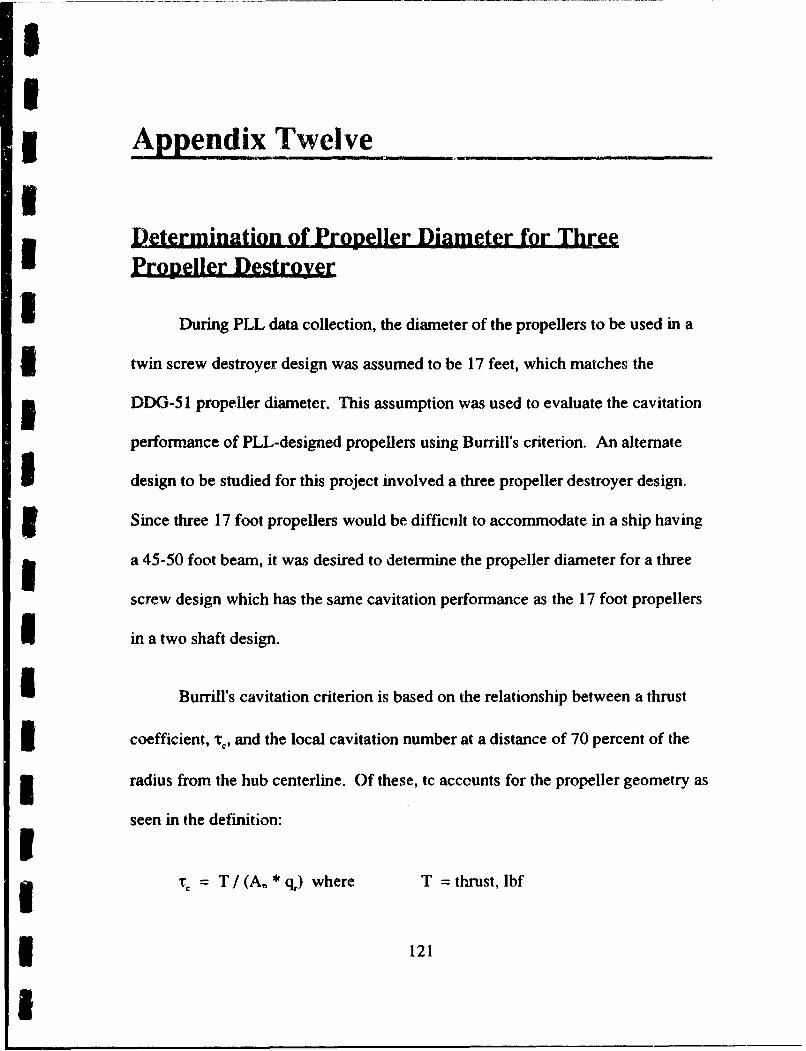
SSI Appendix Twelve
IDetermination of Propeller Diameter for ThreePropeller Destroyer
During PLL data collection, the diameter of the propellers to be used in a
twin screw destroyer design was assumed to be 17 feet, which matches the
5 DDG-51 propeller diameter. This assumption was used to evaluate the cavitation
performance of PLL-designed propellers using Burrill's criterion. An alternate
I design to be studied for this project involved a three propeller destroyer design.
" ! Since three 17 foot propellers would be difficult to accommodate in a ship having
a 45-50 foot beam, it was desired to determine the propeller diameter for a three
screw design which has the same cavitation performance as the 17 foot propellers
I in a two shaft design.
SBurrill's cavitation criterion is based on the relationship between a thrust
I coefficient, T., and the local cavitation number at a distance of 70 percent of the
3 radius from the hub centerline. Of these, tc accounts for the propeller geometry as
seen in the definition:IiT = T / (A. * q,) where T = thrust, lbf
3 121
I
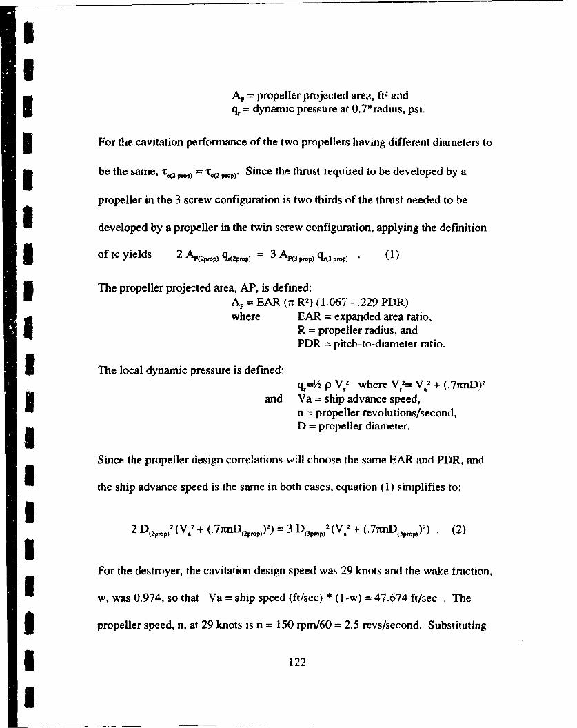
S
Ap = propeller projected area, ft2 andq, = dynamic pressure at 0.7*radius, psi.
SI For the cavitation performance of the two propellers having different diameters to
3 be the same, ".(2 prop) = Xc(3 pro)" Since the thrust required to be developed by a
propeller in the 3 screw configuration is two thirds of the thrust needed to be
developed by a propeller in the twin screw configuration, applying the definition
of tc yields 2 AP( 2P-P) l2prop) = 3 AP3 p-op) q(3 prop) (1)
3 The propeller projected area, AP, is defined:AP = EAR (n R2 ) (1.067 - .229 PDR)where EAR = expanded area ratio,
R = propeller radius, andPDR = pitch-to-diameter ratio.
I The local dynamic pressure is defined-
q,=/2 p Vr2 where V2= V.2 + (.7nmD)2
and Va = ship advance speed,n = propeller revolutions/second,I D = propeller diameter.
Since the propeller design correlations will choose the same EAR and PDR, and
I the ship advance speed is the same in both cases, equation (1) simplifies to:
I2 D(2piop)2 (V. 2 + (.7 lnmD(2prop)) 2) = 3 D(yprp) 2 (V.1 + (.7rnD(3Prop))Y) (2)I
For the destroyer, the cavitation design speed was 29 knots and the wake fraction,
w, was 0.974, so that Va = ship speed (ft/sec) * (l-w) = 47.674 ft/sec . The
5 propeller speed, n, at 29 knots is n = 150 rpm/60 = 2.5 revs/second. Substituting
5 122
I

-- • !these values into equation (2) and assuming a twin screw propeller diameter,
.Dv, of 17 feet yields D<pp = 15.2 feet, which can be fit into a ship with a1 45-50 foot beam,
I
Ii
I
I 123
IISAppendix Thirteen
IComputer Routines for Predicting Off-design Propulsor
SPerformance
3 Prop Performance for Destroyer Design
/* This module is designed to provide performance estimate for several types of DDGpropulsors. It takes as input the propuisor type of interest, propeller geometryinformation generated by the function prop-design and speed for which performance isrequired. It returns the QPC and RPM of the selected propulsor at that speed. Functionsare included which invoke correlations for propeller performance based on data collectedfrom the Propeller Lifting Line computer program. */
#include "propmain.h"
3 void prop-perfomxance(int type-props, int numcruise prop, int n.props, double speed,double idle_speed, double EAR, double PDR, double *QPC,double *rpm)
double thrust ded = 0.945; /* 1-t */double wakefrac = 0.974; /* l-w */double Va; double Dp;double jetQPC~jetjrpm;if(type-props == 9)
jet-performance(speed, &jetQPC, &jet-rpm);*QPC = jetQPC;
*rpm = jet-rpm;return;
if(n.props == 2)Dp = 17;
elseI Dp = 15.2;Va = speed * 1.68781 * wake- frac;iftnumcruise.Aprop == 1)
*124
3
"speed = 1.6 * speed;Va = 16 * Va;*QPC = (efficiency(speed, idle_speed, EAR, PDR, typeprops) * thrust-ded) /
wakefrac;if(type.props == 2 && speed < idle.speed i1 type.props == 6 && speed <
idle-speed)I _
speed = idlespeed;Va = speed* 1.68781 * wake._frac;3 Il*rpm = (Va * 60.)/(J(speed, EAR, PDR, type-props) * Dp);
else3 *rpm = (Va * 60.)/(J(speed, EAR, PDR, type-props) * Dp);
else
*QPC = (efficiency(speed, idle sspeed, EAR, PDR, type_.props) t ,hrustded) /wake_frac;
if(type-props == 2 && speed < idle-speed II type-props == 6 && speed <idle.speed)
speed = idlespeed;Va = speed* 1.68781 * wakefrac;*rpm = (Va * 60.)/(J(speed, EAR, PDR, typeprops) * Dp);-I
elseu •*rpm = (Va 60.)/(J(speed, EAR, PDR, typeprops) * Dp);
return;
/* This function rerurns. the open water efficiency of a selected DDG prop. */
double efficiency(double speed, double idle speed, double EAR, double PDR,ini type-props)
doublc eta;if(type.e_props /* FPP */
eta = ftp.eta(speed, EAR);retura(eta);
5251
if(type-..props =2 && EAR < 0.799) /* CRP *
if(speed < idle-speed)eta = crp eta-low-speed(speed, idle-.speed, PDR, EAR);
elseeta = ifpp1.eta(speed, EAR) -0.052;
retum(eta);
if(type-.props ==2 && EAR >= 0.799) P, CRP *
a ~if(speed < idle..speed)eta = cip-etajow...speed(speed, idle-speed, PDR, 0.799);
elseI ~ ~eta = crp...eta(speed, PDR);retum(eta);
I ~if(type-.props == 3) /* contrarotating *
eta = contra -eta(speed, EAR);return(eta);
3 if(type-~props == 4) f* pre-swiri. stator
eta = preswirl-eta(speed, EAR);3 return(eta);
if(type, -props,- 5) /* ducted FPP ~
eta = ductedj- pp-eta(spmeed, EAR~);return(eta);
if(type-props == 6 && EAR < 0.784) /* ducted CRP ~
if(speed < idle-sptid)eta ducted crp-eta-low_speed(speed, idle-speed, PDR, EAR);
else5 eta =ductedjfpp-eta(speed, EAR) - 0,052;retu~m(eta);
3 if(type-props =-- 6 && EAR >= 0.784) /* dw-ted CRP ~
if(speed < idle-speed)eta = ducted_cwp_eta--low-speed(speed, idl~espeed, PD-R, 0.784);
* 126
elseeta = ducted~srp~eta(speed, PDR);
return(eta);
5 if(type-.props =--7) /* ducted contrarotating *
em~ = ducted-contrA..eta(speed, EAR);3 retum(eta);
if(type-props =-8) /* ducted pre-swirl stator ~
eta = ductedpreswirl~eta(speed, EAR);retum(eta);
retuni(0);
I ~/* This function returns the advance coefficien. at a particular speed for the DDG. *double J(double speed, double EAR. double PDR, int type-.props)
double 3;
I J = fppJ(speed, EAR);return(J),
if(type-props == 2 && EAR < 0.799) /* CR1'P
J = fpp Jspeed, EAR);
return(J);
3 ~if(type-.props =-= 2 && EAR >= 0.799) /* CRP *
J = ctp.,J(speed, PDR);
if(type...props ==3) 1* cmitrarotating *
J = contraJ(speedi, FAR);retun(J);
* 127
ff(type...props == 4) P* pre-swirl stator ~
I 3J = preswirl j(speed, EAR);return(J);
I if(type-props == 5) /* ducted FPP *
3 3= ductedjfppJ(speed, EAR);return(J);
if(type...props == 6 && EAR < 0.784) /P ducted CRP *
J = ducted-fppJT(speed, EAR);Ieu()if(type...props == 6 && EAR >= 0.784) /P ducted CRP *
J3= ducted - rpj(speed, PDR.);ii return(J);
if(type-.props == 7) /* ducted contrarotating *
J r. ducted -contraJ(speed, EAR);return(J)
if(type props == 8) /* ducted pre-swirl stator ~
J = ducted-preswirl J(speed, EAR);retum(J);
retutn(0);
I double fpp~eta(double speed, double ear)
3 ~double aO,aI ,a2,a3,x,eta;aO -0. 291 *ear*ear + 0.273*ear + 0.711;al = .0257*ear*ear - O.0345*ear + 0.0 105;3 a2 = 0.00205*ear*ear + 0.00285*ear - 0.000866;a3 0 .000041 *ear*ear - 0.0000651 *ear + 0.0000214;if (speed < 12.)I eta = a3*pow(l 2.,3.) + a2*pow(1 2.,2.) + alI*12. + aO;
3 128
SI
elseeta = a.3*pow(speed,3.) + a2*pow(speed,2.) + al*speed + aO;
retum(eta);
double crpeta(double speed, double PDR)
double aO,al,a2,a3,x,eta;x = speed;aO = 0.353*PDR + 0.143;al = -0.044*PDR + 0.0672;a2 = 0.00206*PDR - 0.00306;a3 = -0.0000299*PDR + 0.0000416;eta = a3*pow(x,3.) + a2*pow(x,2.) + al*x + aO;retum(eta);II
I double crp-etalow.speed(double speed, double idle-speed, double PDR, double ear)
double aO,al,a2,a3,x,eta,bO,b l,b2,b3,b4,b5;x = speed;bO = 0.00328;bi = 0.0809;b2 = 0.0122;b3 = -0.000982;b4 = -0.0000327;b5 = 0.0000026;if (ear < .799)
I aO = -0.291*ear*ear + 0.273*ear + 0.659;al = 0.0257*ear*ear - 0.0345*eax + 0.0105;a2 = -0.00205*ear*ear + 0.00285*ear - 0.000866;a3 = 0.000041*ear*ear - 0.0000651*ear + 0.0000214;eta = (a3*pow(idlespeed,3.) + a2*pow(idlespeed,2.) + al*idle_speed + aO) *5 (b5*pow(x,5.) + b4*pow(x,4.) + b3*pow(x,3.) + b2*pow(x,2.) + bi *x + bO);
else
aO = 0.353*PDR + 0.143;al = -0.044*PDR + 0.0672;a2 = 0.00206*PDR - 0.00306;
129
a3 = -0.0000299*PDR + 0.0000416;eta = (a3*pow(idle...speed,3.) + a2*pow(idle -speed,2.) + alI *jidle_speed + aO)
(b5*pow(x,5.) + b4*pow(x,4.) + b3*pow(x,3.) + b2*pow(x,2.) + blI*x + bO);
I ~return(eta);
double contra-eia(double speed, double ear)
I ~double, aO,alI,a2,a3 ,x,eta;x = speed;AO = 6.98*ear*ear + 7.35*ear - 1.09;I al = 1.0*ear*ear - 1.09*ear + 0.288;a2 = -0.0455*ear*ear + 0.0494*ear - 0.01 30;a.3 = 0.000625*ear*ear - 0.000679*ear + 0.000177;I if (speed < 12.)
eta = a3*pow(12.,3.) + a2*pow(12.,2.) + al*12. + aO;elseI eta = a3*pow(x,3.) + a2*pow(x,2.) + al*x + aO;
return(eta);
3 double preswirl~eta(double speed, double ear)
double aO,al.,a2,a3,x,eta;I x = speed;aO = -..544*ear*ear + 8.27*ear - 2.32;al = 0.85*ear*ear - 1.32*ear + 0.501;3 a2 = -0.0421l*ear*ear + 0.0654*ear - 0.0248;a3 = 0.00J64*ear*ear - 0.000997*ear +0.000378;if (speed < 12.)I eta = a3*pow(12.,3.) + a2*pow(12.,2.) + aJ.* 12. + aO;else
eta = a3*pow(x,3.) + a2*pow(x,2.) + al*x + a.O;U ~return(eta);
double ducted...fpp-eta(doulle speed, double ear)
double aO,al ,a2,a3,x~eta;I x = specd;
* 130
aO = -1.29*ear*ear + 1.72*ear + 0.208,al. = O.0366*ear*ear - 0.0583*ear + 0.02 13;a2 = -0.00316*ear*ear + 0.00487*ear - 0.00169;03 = 0.00012*car*ear - 0.000182*ear + 0.0000634;if (speed <12.)eta = a3*pow(12.,3.) + a2*pow(12.,2.) + al* 1.2. + aO;
elseI eta = a3*pow(x,3.) + a2*pow(x,2.) + a1*x + aO;retum(eta);
double ducted~crp..eta(double speed, double PDR)
double aO,a1 ,a2,a3 ,x,eta,bO,b 1,b2,b3;x = speed;I aO = -.00106*PDR + 0.762;al = 0.0144*PDR - 0.0287;a2 = -0.000655*PDR + 0.00141;
a3 = 0.0000076*PDR - 0.0000199;eta = a3*pow(x,3.) + a2*pow(x,2.) + alI*x + aO:3 return(eta);
I ~double ductedsCrp...eta low-speed(double speed, double idle~speed, double PDR,double ear)
double aO,al,a2,a3,x,eta,bO,bl ,b2,b3,b4,b5;X = speed;I bO = 0.00328;bi = 0.0809;b2 = 0.0122;3 bW = -0.000982;Mb= -0.0000327;b5 = 0.0000026;3 ~if (ear < .784)
aO = -1.29*ear*ear + 1.72*ear + 0.156;U ~al = 0.0366*ear*ear - 0.0583*ear + 0.0213;a2 = -0.00316*ear*ear + 0.00-487*ear - 0.00169;3 a3 = 0.00012*ear*ear - 0.000182*ear + 0.0000634;
3 131
eta =(a3*pow(.idie..speed,3.) +4 a2"'pow(idle-..speed,2.)+ al*idle_speed + a0 *3 (b5*pow(x,5.) + b4*pow(x,4.) + b3*pow(x,3.) + b2*pow(x,2.) + bl*x + bO);
else
IA aO 0.0106*PDR + 0.762;al.= 0.0144*PDR - 0.0287;a2 -0.000655*PDR + 0.00141;
a3 0.0000076*PDR - 0.00001909;eta = (a3*pow(idlc._.speed,3.) + a2*pow(idle...speed,2.) + at *idle-spleed + aO) ~
(b5*pow(x,ti.) + b4*pow(x,4.) + b3*pow(x,3.) + b2*pow(x,2,) + blI*x + bO);
retum(eta);
3 double ducted_contra eta(double speed, double ear)
double aO,aI1,a2,a3,x,eta:x = speed;aO = -2.42*ear*ear + 2.0*ear + 0.476;al = -0.248*ear*ear + 0.316*ear - 0.104;3 a2 = 0.00557*ear*ear - 0.00836*ear + 0.00323;a3 = 0.0000977*ear*ear - 0.0000716*ear + 0.0000032;if (speed < 12.)Ieta = 3*pow(1 2.,-'1.) + a2*pow(1 2.,2.) + al * 12. + aO;else
eta =n3*pow(x,3.) + a2*pow/x,2.) + al*x + aO;
return(eta);
double ducted~prnswirl...eta(double speed, double ear)
double aO,al ,a2,a3,x,eta;X = speed;aO = -2.l9*ear*ear + 3.18*ear - 0.305;al = O.256*ear*ear - 0.394*ear + 0. 139;a2 =4)0.0137*ear*ear +4 0.02 '11 eai - 0.00748;a3 = 0.000232*ear*ear - 0.000361 *ear + 0.000 129,if (speedJ< 12.)
eta = a3*pow(,121.,3.) + a2*pow(1 2.,2) + al * 12. + aO;I else
* 132
eta = a3*pow(x,3.) + a2*pow(x,2.) + al*x + aO;retum(eta);
double fpp-j(double speed, double ez.)
3 ~double bO,bl,yJ;y = speed;bi. = -0.0l93*ear + 0.00418;3 bO = -O.0638*ear + 1.55;J =bly + b0;retum(J);
3 double crp-J(double speed, double PDR)
double bO,bl,yJ;I y = speed;bi. = -0.00713*PDR + 0.000613;bO = PDR - 0.09;
~ J= b1*y +b0Wretum(J);
3 double contraji(double speed, double ear)
double bO,bl,yJ;y =speed;
bk = -0.000256*ear - 0.0119,bO = 2.62*ear +3.44; J =bI*y +bO;retumr(J)
3 double preswirl-J(double speed, double ear)
double bO,bl,y.,J:y = speed;bl1 = -0.~00i%*ear - 0,007;hO = -0.983*ear + 2.48;
* 133
II
Jbl*y + 0;5retum(J);
S double ducted_fppj(double speed, double ear)
I double bO,bl,yJ;y = speed;bl = -O.000407*ear - 0.0129;bO = -18.5*ear*ear + 26.10*ear - 7.42;J = bl*y + bO;return(J);
I double ducted_.crpJ(double speed, double PDR)
double bO,bl,y,J;y = speed;bl = -0.0245*PDR + 0.0228;
Sb0 = 2.16*PDR - 1.68;J = bl*y + b0;retum(J);I
3 double ducted_contra J(domble speed, double ear)fdouble bO,bl ,y,J;y = speed;bI = 0.00278*ear - 0.013 1;bO = -70.1*ear*ear + 70.7*ear - 15.5;J = bl*y +bO;retum(J);i I
double ducted-preswirlJ(double speed, double ear)
double bO,bl,yJ;y = speed;bI = 0.00122*ear - 0.0107;
3 134
I'
bO = -5.2*ear*ear + 6.97*ear - 0.651;J = bl*y + bO;return(J);I I
PropPerformance for Amphibious Ship Design
/* This module is designed to provide performance estimate for two types of LXpropulsors. It takes as input the propulsor type of interest, propeller geometryinformation generated by the function prop-Aesign and speed for which performance isrequired. It returns the QPC and RPM of the selected propulsor at that speed. Functionsare included which invoke correlations for propeller performance based on datacollected from the Propeller Lifting Line computer program. */
I #include "propjlx.h"
U void prop-performance(int type-props, hat num-cruise-prop, double speed, doubleidlespeed, double EAR, double *QPC, double *rpm)
3dolible thrustded = 0.905; /* 1-*double wakefrac = 0.965; /* l-w I /double Va;double Dp;Dp = 16.;Va = speed * 1.68781 * wakejfrac;if(num-cruise-prop == 1)
speed = 1.6 * speed;Va-= .6 * Va;*QPC = (efficiency(speed, idle-speed, EAR, typeprops) * thrust.ded) / wake_frac;
if(type-props == 2 && speed < idle-speed)I _
speed = idlespeed;Va = speed 1.68781 * wake_frac;* rpm = (Va * 60.)/(J(speed, EAR, type-props) * Dp);
else*rpm = (Va * 60.)/(J(speed, EAR, type..props) * Dp);
else
3 135
I
I
*QPC = (efficiency(speed, idle-speed, EAR, type-props) * thrust-ded) / wake-frac;I if(type-props == 2 && speed < idle_.speed)II
speed = idlespeed;Va = speed * 1.68781 * wake.frac;*rpm = (Va * 60.)/(J(speed, EAR, typeprops) * Dp);
else*rpm = (Va * 60.)/(,(speed, EAR, type-props) * Dp);
)3 }return;
/* This function returns the open water efficiency of a selected LX prop. */
double efficiency(double speed, double idlespeed, double EAR, int type-props)
double eta;if(typeprops = 1) /* FPP*
eta = fpp-eta(speed, EAR);return(eta);
if(type-props == 2) /* CRP */I{if(speed < idle-speed)
eta = crp.etailow.speed(speed, idlespeed, EAR);else
eta = crp eta(speed, EAR);3 } return(eta);
return(O);I/* ITis function returns the advance coefficient at a particular speed for the LX. */
double J(double speed, double EAR, int type-props)
double J;if(type-props == 1) /* FPP *1
I133 1 36
U
J = fppJ(speed, EAR);return(J);
if(type...props == 2) /* CRP *
J = fpp_.J(speed, EAR);retum(J);
return(O);
double fpp...eta(double speed, double ear)
double aO,al ,a2,a3,x,eta;a0 =0.463*ear*ear~ -l.2*ear + 1.331;a aI = -0. 272*ear*ear + 0.424*ear - 0. 165;a2 = 0.0363*ear*ear - 0.0567*car + 0.0221;a3 = -0.001 13*ear*ear + 0.00176*ear - 0.000689;I if (speed < 12.)eta = a3*pow(12.,3.) + a2*pow(12.,2.) + al * 12. + aO;
elseII eta = a3*pow(speed,3.) + a2*pow(speed,2.) + al*speed + aO;retum(eta);
double c~rp...eta(double speed, double ear)
double aO,al ,a2,a3,x,eta;3X = speed;aO = 0.463*ear*ear - 1.2*ear + 1.278;al = -0.272*ear*ear + 0.424*ear - 0. 165;a2 = 0.0363*ear*ear - 0.0567*ear + 0.0221;a3 = -0.001 13*ear(ear + 0.00176*ear - 0.0006899eta = a3*pow(x,3.) + a2*pow(x,2.) + al*x + aO;return(eta);
double cm, -eta-low-speed(douiAo- speed, double idle-speed, double ear)
double aO,al ,a2,a3,x,eta,b0,bl ,b2,b3,b4,b5;
* 137
x = speed;3b = 0.00328;bI = 0.0809;b2 = 0.0122;b3 = -0.000982;Mb= -0.0000327;b5 = 0.0000026;3 '30 = 0.463*ear*ear - 1.2*ear + 1.278;al = -0.272*eai"'ear + 0.424*car - 0. 165;a2 = 0.0363*ear*ear - GO.67*eaix +~ 0.0221;&A5 = -3.00 113 *ear*ear + 0.00 176*ear - 0.000689;eta = (a3*pow(idle~speed,3.) + a2*pow(idle~speed,2.) + al*idle...speed + a(?)*
(b5*pow(y.,5.) + b4*pow(x,4.) + b3pow(x,3.) + b2*'pow(x,2.) + bl*x + bO);U retum(eta);
Joubic fpp.j(double speed, double ear)
I ~double bO,bl,yJ;y = speed;bi = .,.418*ear*ear + 6.28"'ear - 2.36;bO = 102*ear*ea~r - 154*ear + 59.7;J =bl*y +bO,retum(J);
13
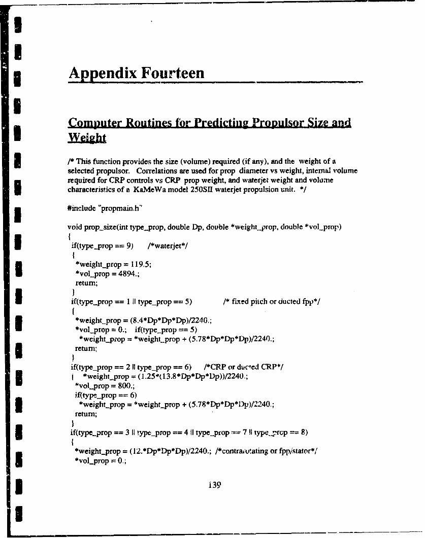
UISAppendix Fourteen
Computer Routines for Predictin'g Propulsor Size and
3 /* This function provides the size (volume) required (if any), and the weight of aselected propulsor. Correlations are used for prop diameter vs weight, internal volumerequired for CRP controls vs CRP prop weight, and waterjet weight and volumeUI characteristics of a KaMeWa model 250S11 waterjet propulsion unit. */
#include "propmain.h"
void prop-size(int type-prop, double Dp, double *weight-prop, double *vol prop)
i if(type-prop == 9) /*waterjet*/
*weiglht-prop = 119.5;
*volprop = 4894.;return;!I
if(type-prop == 1 II type-prop -= 5) /* ftixed pitch or ducted fpp*/
*weight-prop = (8.4*Dp*Dp*Dp)/2240.;*vol-prop = 0.; if(type.prop == 5)*weight-prop = *weight__prop + (5.78 *Dp*Dp*LDp)/2240.;
return;
if(type-prop == 2 11 type.prop == 6) /*CRP or ducted CRP*/*weight prop = (1.25*(13.8*Dp*Dp*Dp))/2240.;
*vol-prop = 800.;if(type-prop == 6)3 ~*weight-prop = *weightpo +N(Iretm;*Wightpr~p *weghtprop + (5.78*Dp*Dp*Dv)/2240.;
return;
if(type-prop == 3 II type-prop == 4 11 type-prop == 7 11 typeprop == 8){*weight-prop = (12.*Dp*Dp*Dp)/2240.; /*contraivtating or fpp/stator*/*vol-prop = 0.;
* 139
U
if(type.,:,p 7 11 type-,.prop =-= 8)3 *weight-.pI.i- * 'weight-prop + (5.78 *Dp*Dp*rDp)/2'240.;ret~irn,
retarn;
14