AN EVALUATION OF NEGATIVE INCOME TAXES WITH HETEROGENEOUS AGENTS

Justin Smith Bachelor of Arts, McMaster University 2003

PROJECT SUBMITTED IN PARTIAL FULFILLMENT OF THE REQUIREMENTS FOR THE DEGREE OF

MASTER OF ARTS

In the Department

of Economics

O Justin Smith 2004

SIMON FRASER UNIVERSITY

April 2004

All rights reserved. This work may not be reproduced in whole or in part, by photocopy

or other means, without permission of the author.

APPROVAL

Name: Justin Smith

Degree: M. A. (Economics)

Title of Project : An Evaluation Of Negative Income Taxes With Heterogeneous Agents

Examining Committee:

Chair: Ken Kasa

David Andolfatto Senior Supervisor

Doug Allen Supervisor

Simon Woodcock Internal Examiner

Date Approved: Tuesday April 6th, 2004

. . 11

Partial Copyright Licence

The author, whose copyright is declared on the title page of this work, has

granted to Simon Fraser University the right to lend this thesis, project or

extended essay to users of the Simon Fraser University Library, and to

make partial or single copies only for such users or in response to a

request from the library of any other university, or other educational

institution, on its own behalf or for one of its users.

The author has further agreed that permission for multiple copying of this

work for scholarly purposes may be granted by either the author or the

Dean of Graduate Studies.

It is understood that copying or publication of this work for financial gain

shall not be allowed without the author's written permission.

The original Partial Copyright Licence attesting to these terms, and signed

by this author, may be found in the original bound copy of this work,

retained in the Simon Fraser University Archive.

Bennett Library Simon Fraser University

Burnaby, BC, Canada

ABSTRACT

In this study I evaluate a negative income tax system set in a simple economy

populated by different types of individuals, whose only choice is a decision about how to

allocate discretionary time between working in the paid labour force and consuming

leisure. In particular, I examine how different skill levels and different preferences for

leisure, both separately and interactively, affect labour supply, earnings, income and

welfare across these different types of individuals. A numerical simulation will predict

the immediate response of these individuals to the sudden implementation of the tax

system, with no attempt to judge the dynamics of the response. The findings are that

there are unambiguously negative labour supply effects for all individuals, which are

worse for those people who either have low skill, a high preference for leisure, or a

combination of both. The effects on income and welfare vary with the type of individual.

DEDICATION

Dedicated to my family and friends.

ACKNOWLEDGEMENTS

First and foremost I would like to thank my committee: David Andolfatto, Doug

Allen and Simon Woodcock for all their help. I would also like to thank all my friends at

Simon Fraser who have helped me along the way.

TABLE OF CONTENTS

. . Approval ............................................................................................................................ 11

... Abstract ............................................................................................................................ 111

Dedication ........................................................................................................................ iv

Acknowledgements ............................................................................................................ v

Table of Contents ............................................................................................................. vi . .

List of Figures .................................................................................................................. vii ...

List of Tables .................................................................................................................. vlll

1 Introduction ..................................................................................................................... 1

2 The Model ........................................................................................................................ 5

3 Calibration ..................................................................................................................... 10

4 Results ............................................................................................................................ 13 ................................................................................................. 4.1 Heterogeneous Skill 13

4.2 Heterogeneous Preference for Leisure ..................................................................... 18 ............................. 4.3 Heterogeneous Skill and Heterogeneous Preference for Leisure 22

5 Discussion ....................................................................................................................... 27

..................................................................................................................... 6 Conclusion 30

Appendices ........................................................................................................................ 31 ..................................................................................................... Appendix A: Figures -32

........................................................................................................ Appendix B: Tables 41 ............................................................................................... Appendix C: Gauss Code 46

Bibliography ..................................................................................................................... 62

LIST OF FIGURES

Figure 1 . The Negative Income Tax ................................................................................. 32

Figure 2 . After Tax Income with Heterogeneous Wage ................................................... 33 Figure 3 . Earnings with Heterogeneous Wage ................................................................. 33

Figure 4 . Welfare with Heterogeneous Wage .................................................................. 34

Figure 5 . Welfare Cost with Heterogeneous Wage .......................................................... 34 Figure 6 . Equilibrium Labour Supply with Heterogeneous Wage ................................... 35

.............................. Figure 7 . After Tax Income with Heterogeneous Leisure Preference 35

Figure 8 . Earnings with Heterogeneous Leisure Preference ............................................ 36

Figure 9 . Welfare with Heterogeneous Leisure Preference .............................................. 36 ................................... Figure 10 . Welfare Cost with Heterogeneous Leisure Preference 37

Figure 1 1 . Equilibrium Labour Supply with Heterogeneous Leisure Preference ............ 37 Figure 12 . After Tax Income with Hetergeneous Wage and Leisure Preference ............. 38

......................... Figure 13 . Earnings with Heterogeneous Wage and Leisure Preference 38 ......................................................................... Figure 14 . Total Taxes Paid and Subsidy 39

Figure 15 . Equilibrium Labour Supply with Heterogeneous Wage and Leisure Preference ..................................................................................................... 39

........................... Figure 16 . Welfare with Heterogeneous Wage and Leisure Preference 40

Figure 17 . Welfare Cost with Heterogeneous Wage and Leisure Preference .................. 40

vii

LIST OF TABLES

Table 1 . Model Results with Heterogeneous Wage ......................................................... 41

Table 2 . Model Results with Heterogeneous Leisure Preference ..................................... 41 ............. Table 3 . Model Results with Heterogeneous Wage and Preference for Leisure 42

Table 4 . Model Comparison with Data for Heterogeneous Wage ................................... 44 ......... Table 5 . Model Comparison with Data for Heterogeneous Preference for Leisure 44

Table 6 . Model Comparison with Data for Heterogeneous Wage and Preference for Leisure ......................................................................................................... 45

... Vl l l

1 INTRODUCTION

For decades, economists have been studying the issue of poverty, specifically,

how to design a mechanism to reduce the number of people having very low incomes.

The most well-known of these mechanisms is what some call the "traditional" welfare

system where, individuals are provided with a sum of money, which is decreased dollar

for dollar with increases in income.' Recognizing the obvious work disincentive of such

a policy, economists have studied a variant of the traditional welfare system - the

negative income tax.

Although popularized by Milton Friedman in his 1962 book "Capitalism and

Freedom," precursors to negative income taxes (NIT) can actually be dated back a couple

of centuries. Since that time this type of policy, commonly referred to as guaranteed

annual income, has been subject to much research as a mechanism to alleviate poverty.

The majority of these studies have been conducted since the 1960's. Over these past four

decades, there have been many commissions and many governments in Canada and the

United States proposing variants of the NIT system as part of their political agendas.

Despite this extensive amount of research, there has still not been a consensus among

policy-makers and academics as to whether an NIT, or a variant thereof, is an effective

policy in alleviating poverty while providing adequate work incentives.

To understand the reason for the lack of consensus, a quick review of the theory is

necessary. There are varying designs of the program, but all have the same basic idea:

' Many people refer to a tax-back rate of 100% as a "traditional welfare regime." There are other schemes with lower tax-back rates, but this paper will follow in that trend.

individuals are guaranteed a basic annual income by the government. If they choose not

to work in the paid labour force, then their income is simply the amount of the guarantee.

If, however, an individual does choose to do paid work, then that person's income is

taxed at a positive rate and subtracted from the basic income guarantee to determine the

amount of benefit the individual will receive. For example, if the guaranteed basic

annual income was $5,000, and the individual earned $1,000 in the paid labour force, and

was subject to a 50% tax rate (typically called the reduction rate), then the benefit for this

person would be $4,500. In this example, for every dollar the individual earns, his

benefit is reduced by $0.50.

This benefit will be a positive amount as long as the after-tax earnings are below

the annual income guarantee. The point at which they are both equal is normally referred

to as the break-even point. Typically, when a person is below this threshold they are

eligible for the NIT program, if they are above the break-even point, they are ineligible.

Once ineligible, they return to the regular tax system. One can now see that the term

"negative income tax" refers to the situation where an individual receives a net benefit

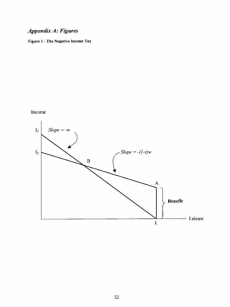
from the government. Figure 1 shows a graphical representation of the textbook NIT

policy. Line LI1 represents a traditional welfare regime, while line A12 represents an NIT

with some tax rate z below loo%, and a basic benefit equal to the distance LA. Point B

is the break-even point in the NIT system. Note that here income and consumption are

interchangeable.

Unfortunately, the theory behind NIT suggests some potential drawbacks. The

positive work incentives of an NIT only apply in a world where a welfare system already

exists; introducing an NIT system in a world where there was no previous welfare system

yields unambiguously negative labour supply effects. First, there is an adverse effect on

labour supply of low-income individuals, taking leisure as a normal good. The income

effect of this system is to induce the individual to work less, given that income is now

higher for this individual at all hours of work below the break-even point. Furthermore,

since each extra dollar earned in the labour force is taxed away - i.e. the cost of leisure is

lower - the individual now has even more incentive to work less (the substitution effect).

These two effects combine to produce a strong disincentive to increase work hours for

those individuals who are receiving a net subsidy from the NIT.

The issue of the amount of the guarantee provides some problems also. For the

government to promise a high amount of basic annual income could be very costly if

there are a large proportion of people eligible for the NIT program. The government

could simply reduce the basic benefit in that case, but if the guaranteed income were

lowered so much that it became insufficient, then this policy would not achieve its goal of

poverty reduction.

Fortunately, it is possible that this work disincentive effect could be very small

and insignificant; also, people could use the extra leisure time they are consuming to

engage in productive job search activities. Finally, comparing the NIT regime to other

welfare designs may actually lead to increased work incentives relative to the

alternative^.^

The discussion of the theoretical implications provides some important insights

into the possible consequences of this poverty-reduction scheme, and begs the question:

- - -

2 Dwayne Benjamin and Morley Gunderson and W. Craig Riddell, Labour Market Economics: Theo y, Evidence and Policy in Canada, 5' ed. (Toronto: McGraw-Hill Ryerson Limited, 2002), 84.

Would the model's predictions be dissimilar for different preferences and skills? Indeed

they are, and the goal of this paper is to examine to what extent this heterogeneity has an

effect on the sudden and unanticipated introduction of an NIT.

Within this context, I propose to evaluate a negative income tax system in a

simple economy populated by different types of individuals, whose only choice is a

decision between working in the paid labour force or consuming leisure. In particular, I

will be examining how different skill levels and different preferences for leisure, both

separately and interactively, affect labour supply, earnings, income and welfare across

these different types of individuals. A numerical simulation will predict the immediate

response of these individuals to the sudden implementation of the tax system, with no

attempt to judge the dynamics of the response. Intuition suggests that those individuals

with the lowest wage and the highest preference for leisure will enjoy the highest amount

of welfare fiom the NIT system. Conversely, individuals with a high wage and a low

preference for leisure will like the NIT regime the least compared to the other types of

individuals in the model.

The paper will be structured as follows: Section 2 describes the model and

provides the equation that characterizes the equilibrium labour supply. Section 3

discusses the calibration of the parameters within the model to some realistic values

based on previous studies. Section 4 provides the results of the model using output from

gauss. Section 5 discusses some of the implications of the results presented, and Section

6 concludes.

2 THE MODEL

The model used in this paper is slightly different than the basic model described

above, but still captures the essence if the NIT design. The difference is that instead of

having a set benefit rate and an eligibility criterion, this model assumes that all

individuals pay a positive amount of income tax, and are subsequently given a subsidy

from the government that is equal across all agents. Notice that this still retains the major

elements of the NIT system: There is a guaranteed annual income equal to the

government subsidy if the individual chooses no hours of work. As individuals increase

their work hours above zero, there exists a point at which the income tax paid by

individuals will exceed the amount of subsidy they receive - this is the break-even point

in this model. In fact, the model used here closely resembles a universal demogrant,

which is another type of guaranteed annual income policy.

Individuals maximize utility over two goods, consumption and leisure, with the

following utility function3:

The parameter cp represents the individual's preference for leisure over

consumption. Higher values of cp represent a higher weight being placed on leisure

relative to consumption. The subscript j = L, M, H placed on this variable refers to its

three possible values: low medium and high. Discussion of the quantitative

This utility function produces smooth, convex indifference curves. We can thus be certain that we have a unique interior solution.

characteristics of these three values follows in the next section. The parameter q is the

curvature parameter on leisure. The higher is the value of this parameter, the less willing

this individual will be to trade leisure for consumption. In other words, the higher the

value of q, the more consumption and leisure are complements, the lower the value, the

more they are substitutes. Note that when q is equal to zero, utility is linear in

consumption and leisure, and non-linear otherwise.

Individuals can choose to allocate their fixed amount of time only to work or to

leisure in this model, thus:

Where work, in this case, refers to participation in the paid labour market, and

leisure refers to any other activity, including activities such as: unpaid work, labour

market search, etc. Individuals are endowed with an amount of time equal to 1.

Individuals are subject to a budget constraint:

c, I (1 - z) win, + S (3)

where c is consumption, T is a distortionary income tax, w is the wage rate, n is

employment and S is a per-person subsidy given to all individuals by the government.

This constraint binds the individual to consume an amount equal to or less than his after-

tax income. The subscript i = L, M, H on wages refers to three possible levels, low

medium and high, the numerical values of which are discussed in the following section.

Notice that since there is no saving in this model, individuals will consume all of their

after-tax income.

Finally, the government in this model has only one role, which is to collect tax

and redistribute its total collection equally to all individuals. Thus, the government's

budget constraint is given by:

With the weighting parameter h, the government's budget constraint incorporates

that approximately 25% of individuals are high-school dropouts, 50% are high-school

graduates and 25% are university graduate^.^ The wage rates in the model will be

calibrated to match the earnings differentials among these three educational groups.

The goal of this paper is a) to examine the effects of changes in the preference

parameter <p, b) to estimate the effects of changes in w, and c) to study the changes

resulting from an interaction of the changes in those two parameters. To accomplish this

end, the labour supply function of each agent must be found. To simplify the

maximization, the constraint in equation (3) is substituted into equation (I), the

individual's utility function. The resulting equation:

is then maximized with respect to nij to yield the agents' labour supply functions.

The first order conditions of this maximization exercise are:

4 David Andolfatto and Christopher Ferrall and Paul Gomme, "Lifecycle Learning, Earning, Income and Wealth," Maunscript: Simon Fraser University (2000), 1.

7

where the solutions to this system of equations characterize labour supply choices

nil*(=). Due to the non-linearity of the utility function, the first-order conditions for this

problem are a series of non-linear functions, which cannot be solved analytically, thus a

numerical estimation procedure will be used. Depending on the number of different

values for the leisure parameter and wage parameter, we will have i*j different first order

conditions, plus the government budget constraint. A natural question to ask is why did I

not specify the utility function so that the solution would be easier to characterize? The

reasoning is that the labour-leisure decision makes much more sense as a non-linear

decision.

It is natural to think that a person's labour-leisure choice has the diminishing

MRS property, that is, that given that a person has almost no leisure, he would be willing

to trade a lot of income for a little more leisure, and so on. The utility function in this

paper generates smooth, convex indifference curves which possess exactly this property.

Another nice property is that the solutions to this problem are interior. It would make

less sense, for example, to use a linear specification, which would say that a person is

equally willing to trade income for leisure regardless of how much of each he already

has. Furthermore, a linear specification can only lead to either non-unique or corner

solutions.

With the equilibrium so characterized, we can construct the Indirect Utility

fimction, which will be used to calculate changes in welfare associated with changing the

tax rate:

where cij* and is* are consumption and leisure choices respectively evaluated at

their equilibrium levels.

Now that the solution equations have been characterized, it is time to choose

values for the parameters to reflect real-world observations.

3 CALIBRATION

There are four parameters in the model that need to be calibrated. First, z, the

value of the tax rate will be a 10-point grid: z E (0, 0.1, 0.2, 0.3, 0.4, 0.5, 0.6, 0.7, 0.8,

0.9). The purpose of this is to examine first the difference between having an NIT

against a laissez-faire regime, and second to observe the effects of an increase in the tax

rate as it gets closer to 1 (the traditional welfare regime).

The value for q is chosen to be 1.5. This is a standard choice for this taste

parameter.5

The value of <p for an average individual is chosen to be 1.48, which reflects the

fact that in the data6, average individuals spend about 35% of their discretionary time in

the paid labour market and 65% of their time in leisure activities. This value will be

considered to be the median value for this taste parameter. The low value is chosen to be

0.84 and the high value 3.52. These values are calibrated to match the fact that,

according to the distribution of hours worked per week, the first third of individuals

spend about 20% of their time working, and the last third spend about 46% of their time

working.'

5 David Andolfatto and Christopher Ferrall and Paul Gornme, "Lifecycle Learning, Earning, Income and Wealth," Maunscript: Simon Fraser University (2000), 9.

6 The source data for this study is a 10% random sample of the 1996 Canada Census individual file. ' To get these values, I took the variable for hours worked per week and sorted it from lowest to highest. I

then separated it into three equal groups which 1 define to be the people with high, median and low preferences for leisure respectively (i.e. low, median and high preferences for work). I then calculate the average hours worked in each group and solve for the value of cp using the first order conditions.

Finally, w is calibrated to match the earnings distribution over three different

education types: high-school dropouts, high-school graduates and university graduates.

From the data, the values of average earnings were calculated for these three groups.8 In

particular, the earnings values reflect only those individuals aged 24-65 who worked

positive hours during the year. Furthermore, observations that were missing were

exc l~ded .~ From this exercise, it was determined that w E (10.34, 12.63, 17.921, where

the numbers are expressed as hourly wage rates.

Some justification is in order for the groups selected in this calibration. First, the

age group was chosen because to compare between groups, it is necessary that most

individuals have finished all of their schooling and begun careers. It is reasonable to

assume that by the age of 24, the university graduates have completed their (bachelor's)

degrees and found employment. Since this paper is concerned more with labour supply

at the intensive margin (i.e. time spent in the labour force), and less at the extensive

margin (i.e. the binary choice of being in or out of work), it is better to have calibrated

the wage parameter with those people who are actually working. For this reason, only

those individuals who worked positive hours were included.

One last note about the calibration of the wage parameter is that there has been

almost no disaggregation in the data (except by what has already been noted in the

previous paragraph). The reader should keep in mind that these values of the wage

8 The variable for highest degree, certificate or diploma (dgreep) was the variable of choice in thls calibration. From the Census survey, those who answered "No degree, certificate or diploma" form the high school dropout group; those who answered "Secondary (hlgh) school graduation certificate or equivalent" form the high school graduate group; those who answered "Bachelor's degree(s)" form the university graduate group.

9 Of course, there is the possibility that there is some systematic reason why certain persons have missing observations and by throwing them away I throw away information. However, there has been no regression done here; simple averages were calculated, so including these observations would have added no useful information.

parameter would be significantly different when comparing females versus males for

example. This will be discussed later in section 5.

With the model so calibrated, it is now time to examine first the effects of the NIT

on individuals with heterogeneous skills and homogeneous preferences for leisure.

Following that, I will study the opposite case where skill is the same across agents, but

their preferences for leisure are heterogeneous. Subsequently, I will examine the effects

when both wages and preferences for leisure are heterogeneous.

4 RESULTS

4.1 Heterogeneous Skill As mentioned in the last section, there will be three values for the wage, which

are calibrated to match earnings differences among high school dropouts, high school

graduates and university graduates. The parameter cp is set here to its median value, 1.48.

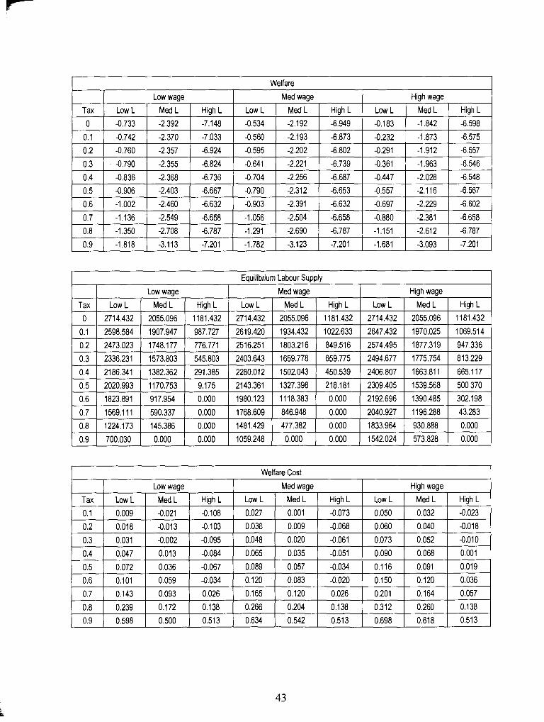
The numerical results of this simulation can be found in Table 1.

Figure 2 plots the after-tax income of the three types of people in this model

economy. As expected, for all individuals, after-tax income is decreasing in the tax

rate.'' Notice that the steepness of the function is greatest for the high-wage individual,

which is to say that marginally, this type of person is most affected by increases in the tax

rate. Intuitively this makes sense because with the NIT regime that has been constructed

in this paper, the high-wage individual is basically subsidizing the lower-wage

individuals. The NIT has a waterfall effect, which is to say that the highest income

individuals are providing subsidy to all individuals below them. However, this is not

always necessarily true, since it is dependent on the concentration of a certain income

group within the population. The population distribution here was calibrated so that

high-school graduates represent 50% of the population, so conceivably there could be

wage structures where the high school grads would actually be subsidizing both higher

income groups and lower income groups.

10 Remember that given the budget constraint for the individual, after-tax income is equivalent to consumption in the NIT regime, while consumption at a zero tax rate (i.e. without the NIT regime) is equivalent to earnings. Thus, any comparison of after-tax income to earnings is the same as comparing consumption with and without the NIT regime. Thls follows from the fact that there is no saving in this model.

What about the effect if the implementation of the regime? One way to gauge the

result is to compare the after-tax income to the earnings for each type of individual.

Figure 3 plots the earnings of the three types of wage earners. For the low-wage

individual, the earnings function lies below the after-tax income function at all levels of

the tax. In fact, the more the tax rate increases, the greater is the gap between these two

functions. Therefore, in this regard, the low-wage individual benefits greatly from the

welfare regime.

For the median-wage individual, the earnings function also lies entirely below the

after-tax income function. Both he and the low wage individual are being subsidized by

the high wage individual. The gap between these two functions widens as the tax rate

rises, but not by much; that is, his labour supply decisions are such that he is paying

almost as much into the subsidy fund as he is receiving.

Finally, for the high-wage individual, earnings are always higher than after-tax

income, with the gap widening at each level of the tax rate. This individual enjoys

consumption most without the NIT system no matter what the tax rate. This result is not

surprising since this type of person contributes a disproportionately high amount to the

total subsidy given his wage is 41% higher than the level below him and 73% above the

lowest wage earner. Thus, what we are seeing here is the waterfall effect that was

described above.

In terms of consumption, the model predicts that for most of the population (about

66% of individuals) the NIT regime is beneficial, and for the other 34% (the high wage

earners) it is detrimental. To get a quantitative estimate of exactly how much better or

worse off these individuals may be from this NIT regime, a welfare function has been

constructed, and is presented in Figure 4.

The first thing to notice is that both the median-wage and low-wage individuals

maximize their welfare at positive tax rates. For the low-wage individual, this tax rate is

around 35%, and for the median wage individual, it is about 20%. This is not true for the

high-wage individual who maximizes his welfare at a zero tax rate. Consequently, using

the welfare function, we can reiterate what was discussed previously with the

consumption comparisons: The low-wage individual likes a NIT regime with a very

heavy tax burden. The reason is that this type of individual contributes relatively little to

the government in terms of taxes, so he stands to gain the most from the subsidy. On the

other hand, the high-wage individual is exactly the opposite, and the median-wage

individual is somewhere in between, leaning slightly towards a positive tax rate.

Although the previous paragraph shed light on exactly how high of a tax rate

would be most preferred by each type of individual, it did not tell us exactly how much

would be gained or lost by the implementation of the NIT regime, and also with

successive increases in the tax rate. For this reason, the compensating variation is used to

provide the percentage of consumption that the individual would have to be given to live

in the progressively burdensome NIT regime. Figure 5 shows these percentages at

increasing levels of the tax rate. It is showing us essentially what the individual would

pay to not have the negative income tax redistribution policy imposed on him, that is,

where he is indifferent between having the negative income tax or no redistribution

policy at all. Intuitively, this should be equal to the losses he expects to generate when he

compares this to the world with no redistribution policy. If there are any gains, then it is

also clear that the individual would be willing to pay that amount to have the policy

imposed on him.

With that in mind, there are a few interesting things to notice in Figure 5. First,

the low-income individual is actually willing to give up a significant amount of

consumption to live in the NIT regime up to a tax rate of about 35%. The median-income

person is virtually indifferent between a tax rate of 20% and no NIT regime. Finally, the

high-wage individual will always need to be compensated a percentage of consumption to

live in a world where the NIT exists. This can be most easily seen on the graph where the

line crosses the horizontal axis.

One final note about Figure 5 is that the cost of a marginal increase in the tax rate

is increasing at an increasing rate. For example, the low-wage individual would have to

be compensated 25% of consumption to live with a tax rate of 0.8, but would have to be

compensated 61% of consumption to live with a tax rate of 0.9. The results are not

surprising since at low levels of tax, the low-wage individual is contributing little and

receiving much, so he will enjoy the welfare state. At the high tax level, the low-wage

person is contributing nothing, but his subsidy is quickly decreasing, so he will not like

the increasing tax burden. As the tax rate increases, all individuals supply less and less

labour in equilibrium, the amount of the subsidy declines, and the individuals lose an

increasing amount in terms of consumption.

What about the labour supply effects? Judging by the results using this model,

there is only a negative incentive effect. Looking at Figure 6, we can see that for all

individuals, the equilibrium labour supply function is always decreasing (at an increasing

rate) in the tax rate. The low-wage individuals have strongest disincentive effect, and

will actually supply no labour once the tax rate reaches about 90%. The other individuals

will supply a positive amount of labour even at very high tax rates, although it is not a

very high amount (as low as 0.7% of their available time). See Table 1 for the tax

elasticity of labour supply.

The substitution effect here is negative since the increase in the tax rate makes the

cost of leisure lower by essentially lowering the wage; hence the incentive is to consume

more leisure. There are two income effects. First, the increase in the tax rate reduces

income at some given number of hours of work, and since leisure is a normal good, he

consumes less of it - and more work. Second, the subsidy provides extra income to

individuals at some given number of hours of work, which decreases work incentives.

What we are seeing here is either a dominant substitution effect or that the net income

effect is working in the same direction as the substitution effect. In any case, individuals

unambiguously choose more leisure at higher tax rates.

The implications of the adverse labour supply effect are somewhat discouraging.

At positive tax rates, the equilibrium labour supply of all individuals is lower, with the

strongest disincentive effect shown by the lowest-wage level. This suggests that the NIT

system has strong negative incentives, which has concerned many researchers in the past,

with the added problem that everyone will supply less labour in equilibrium, not just the

low-wage individuals. The NIT will be evaluated for its redistributive qualities in section

Now that the theoretical implications have been considered, it is usehl to see how

the model's predictions match up with the data. Table 4 presents this comparison for

after-tax income, earnings and subsidy using model results with a flat tax rate of lo%."

The comparison shows that the hypothetical NIT system actually does not do a terrible

job in replicating the real world data, with the obvious exception of the level of the

subsidy.

The general observations are that the model under-predicts the level of earnings

and labour supply hours, and over-predicts the after-tax income and the level of the

subsidy. It must also be noted here that the hypothetical NIT at the 10% tax level is the

best at generating values close to the data. At other tax rates, the subsidy prediction in

particular is much higher than is observed in the data. Nevertheless, the most promising

part of the model is that it captures the fact that in the real world, people with higher

levels of education tend to have higher levels of earnings and after-tax income; In fact,

no matter what the tax rate, the model results possess this feature.

4.2 Heterogeneous Preference for Leisure Now that we have seen the results of the NIT system on different skill levels, it is

time to switch to a comparison across preferences, specifically that for leisure.

Remember that in the section on calibration, it was noted that the average person spends

about 113 of his time in the labour force, which led to cp = 1.48, and that the low and high

values are taken to be 0.84 and 3.52 respectively. Results from this simulation are

presented in Table 2.

The conclusions are much the same as with the different values of skill, which is

to say that the individuals who enjoy leisure the most will have the highest preference for

I I It must be noted here that the Census data did not contain a variable for total taxes paid by individuals. Thus, I had to approximate the after-tax income in the data. To accomplish this end, I used the federal marginal tax rates (16% for first $32,183 and 22% between $32,184 and $64,368) for 1996 and applied them to the individual's total income.

the NIT system, and the strongest negative equilibrium labour supply effect. Figure 7

shows the after-tax income of the three types of individuals at increasing values of the tax

rate. As expected, the person that enjoys leisure the least (or work the most) has the

highest value of after-tax income, while the person who enjoys leisure the most has the

lowest after-tax income. So it follows that the person with the low preference for leisure

enjoys the most consumption at all levels of the tax rate, with the exception that in the

limit as T + 1 everyone converges to a zero level of consumption. The reason for this is

that labour supply goes to zero for all individuals as T + 1. Intuitively, this is

reasonable: why would anyone work if all of the earnings are taxed away?

Comparing once again the after-tax income functions in Figure 7 to the earnings

functions in Figure 8 for each individual, we see nearly the same results as in the

previous subsection. The individual with the highest preference for leisure has the

earnings function lying below the after-tax income function at all levels of the tax rate,

with the gap widening as the tax rate increases. The median-preference-for-leisure

individual has an earnings function slightly below the after-tax function and the low-

preference-for-leisure individual has his earnings function always above the after-tax

income function. The intuition behind this result is that the person who enjoys work the

most is subsidizing those who prefer work less, via the waterfall effect described

previously.

Note that there is a slight upward-sloping portion to the after-tax income function

of the person with the high preference for leisure between a tax rate of 60% and 70%.

This results from the fact that after 60%, this individual drops out of the labour force, and

that his subsidy at a tax rate of 70% is higher than his after-tax income at the lower tax

rate. This also accounts for the funny shape in the welfare cost function.

The welfare functions for the three types of individuals, shown in Figure 9, are

once again maximized at different values of the tax rate. For the person with the highest

preference for leisure, welfare is maximized at a tax rate of about 60%, while the person

with the median preference for leisure maximizes welfare at a very low tax rate in the

range of about 5%. Not surprisingly, the person with the lowest preference for leisure

maximizes welfare at a zero tax rate.

Quantifying the welfare costs, Figure 10 shows that it is always costly in terms of

consumption to increase the tax rate marginally by 10% for the median and low

preference for leisure individuals, while the person with the high preference for leisure

would be willing to give up consumption for such marginal increases up to 60%. Yet

again, these functions are increasing at an increasing rate so that at very high tax rates,

the marginal increases in the tax rate become very costly for individuals. The logic is

that everyone is receiving a lower and lower subsidy at high tax levels. Those still

supplying labour are paying an increasing share, so their welfare cost is the highest.

Those who are not supplying labour are only receiving the subsidy as their income, which

is in decline, so their welfare costs are on the rise.

Finally, examining the labour supply effects, Figure 11 shows that indeed there is

a decreasing equilibrium labour supply effect of increasing the tax rate. The individual

with the highest preference for leisure will stop supplying labour at a tax rate of 60%,

while the other two types will always supply a positive amount in equilibrium. The

income and substitution effects are identical to the ones states in the previous section.

See Table 2 for the tax elasticity of labour supply.

This has potential negative consequences for the NIT theory. The homogeneity

assumption that characterizes the theory of the NIT does not account for the negative

equilibrium labour supply effects on different types of individuals. We see now that

there are in fact significant differences in equilibrium labour supply effects across

individuals with different preferences, which could make the negative effects we saw

with the different wages even more negative. In fact, one could predict now that an

individual with a low wage and a high preference for leisure will experience very

negative labour supply effects of the increasing tax rate. The implications for the NIT

policy are quite different from those when we only have skill differences. This will be

discussed below in section 5.

The comparison of the NIT at a 10% tax level with the data is presented in Table

5. As with the results from the heterogeneous wage, the hypothetical NIT system does a

remarkable job in predicting the earnings and after-tax income, but a fairly poor job in

predicting the level of the subsidy and a mediocre job in prediction labour supply hours

per year. The second to last point is not terribly surprising given that fact that in the

observed data, the level of government transfers to individuals is not uniform across all

individuals. Still, if we were to average the level of the real world subsidy across the

three leisure-preference groups, the model predicts values that are much too high.

The model does a very good job at mimicking the fact that people with a high

preference for leisure tend to earn less and receive less after-tax income than people with

a low preference for leisure, in spite of the fact that it under-predicts earnings and after-

tax income levels.

4.3 Heterogeneous Skill and Heterogeneous Preference for Leisure Now that differences in skills and preferences for leisure have been examined

within an NIT model separately, the focus will now shift to the interactive effect of these

differences. Specifically, skill and preference for leisure will differ quantitatively in the

same manner as above: w E (10.34, 12.63, 17.921, cp E (0.84, 1.48, 3.52). Thus, there

will be nine types of individuals in this simulation. The numerical results are presented

in Table 3.

Figure 12 plots the after-tax income functions of the nine different types of

individuals. First, as predicted, the person with the lowest after-tax income is the low-

wage, high preference for leisure individual, while the highest after-tax income function

is exhibited by the high-wage, low leisure preference individual. There are a couple of

interesting things to observe in Figure 12. First, it is the type of wage category that has

the biggest impact on how much a person earns, while the leisure preference has a much

smaller effect. It is easy to see that despite their differing preferences for leisure, the high

wage individuals have after-tax income functions that lie a good deal above the after-tax

income functions of any other wage category. This reflects the fact that the university

graduates do earn much more than the other two categories, so it is expected that this will

always have a pronounced effect in this analysis.

Another note is the cluster of lines amongst the low and medium wage earners

with their differing preferences for leisure. It shows that the medium-wage, high leisure

preference persons and the low-wage, low leisure preference individuals will have almost

identical responses to the redistribution policy. This is intuitively clear: although a

person may be earning a low wage, his distaste for leisure may drive him to work so

much that he earns almost the equivalent to someone who does not enjoy working so

much, but earns more money.

The final observation in Figure 12 is that the high-wage, low preference for

leisure individual has the steepest after-tax income function, while the low-wage, high

preference for leisure individual has the shallowest after-tax income function. This says

that on the margin, the former individual is hurt more by increases in the tax rate, while

the latter is hurt the least. The other individuals lie somewhere in between. As before,

after-tax income goes to zero as T -+ 1, since as the tax rate approaches unity, no

individual will supply labour.

Comparing the after-tax income to the earnings shown in Figure 13, all low-wage

individuals have an after-tax income function that lies above the earnings function. Thus

no matter what their preference for leisure, low-wage individuals have significant gains

in consumption from the imposition of the NIT regime. The median wage individuals

experience a very similar difference, with the exception of the person with the low

preference for leisure, who actually experiences higher earnings than after-tax income

over all values of the tax rate. Finally, the high-wage individuals all display after-tax

income functions that lie below their earnings functions.

Once again we can decipher who is a subsidizer and who is a subsidizee from the

results of this simulation. What is observed is that the high-wage persons and the

medium-wage, low leisure preference person are subsidizing the five types of people

below them. That is, we have the four top earners providing assistance to the five lowest

earners. To gain some perspective on the quantitative aspects of the amount of the

subsidy, a quick inspection of Figure 14 gives a nice picture of who is really losing the

most with this policy.

This graph shows the individual contributions to the government for each of the

nine types of people, as well as the per-person subsidy each of them receives (the dashed

line). The most striking feature of this picture is the distance between what the high-

wage, high leisure preference individual pays in taxes, and what he receives in subsidy,

especially at very high tax rates - this is reflective of his strong desire to work and his

extra incentive to do so given to him by high wages.

Another prominent feature of this graph is that the median-wage, low leisure

preference person has a tax payment function that is almost identical to the subsidy

function, except at very high levels of tax. This means that he is at the break-even point

and will be indifferent to this policy for the most part.

Finally, the lower wage, higher preference for leisure individuals all have tax

functions below the subsidy functions, with some of them not paying any amount into the

tax function and reaping the full amount of the subsidy paid by the rest of the people in

this simulation economy. The implications of this will be discussed in the following

section.

The labour supply effects are as expected. The lower wage, higher preference for

leisure individuals begin to work substantially less even with low levels of the tax

because they are receiving more and more subsidy, while working less and contributing

less to the government. The tax elasticity of labour supply is presented in Table 3.

Some even opt to stop supplying labour, as can be seen in Figure 15. The NIT system

falls apart once people stop supplying labour in equilibrium because the high wage

individuals are paying a disproportionately high amount to the government, and since the

subsidy is distributed equally to all individuals, they receive little in return. This is in fact

the major incentive problem facing this type of redistributive policy.

The welfare functions are shown in Figure 16. There are some interesting things

to notice here. First, for a wide range of tax rates, the welfare functions for all

individuals are fairly flat. That is, not much welfare is lost by any individual by

increasing the tax rate at very low levels. Second, at a tax rate of about 55%, welfare

starts to drop very rapidly, since nobody in the economy prefers a very high tax rate. The

intuition behind this is that once the tax rate is raised to such a high level, the total

amount contributed to the subsidy fund declines, and so even those people who are

supplying zero hours of labour will dislike a higher tax rate because their total subsidy is

declining.

Not surprisingly, the low-wage, high preference for leisure individual maximizes

his welfare at a very high tax rate, around 55%. The reason for this is the same as

discussed above, which is to say that the redistribution done by the NIT system gives all

individuals a greater level of welfare since the amount of the per-person subsidy is very

high at low tax levels.

It must be noted here that the results hinge crucially on the assumption that the

population is distributed unequally in skill.12 The same simulation yields much different

results when the individuals are distributed equally in the population.

12 Remember that the model was calibrated so that 25% of individuals are high school dropouts, 50% are high school grads and 25% are university grads.

25

The welfare cost functions, shown in Figure 17, exhibit the same shape as they

did when heterogeneity was examined separately. Interestingly, at very high tax rates,

all individuals experience about the same welfare cost in terms of percentage of

consumption. This can be explained by the fact noted above that as z + 1, consumption

across individuals is getting closer, thus is makes sense that the cost of marginal increases

in the tax rate are about the same.

Finally, comparing the model at a 10% tax rate with the data yields some

interesting insights.I3 As with the previous two sections, the model captures the ordering

of earnings and after-tax income levels well. In this case we see that the person that likes

work the most and earns the highest wage has the highest level of after-tax income and

earnings, and vice versa for the person who likes work the least and earns the lowest

wage. Also like the previous two sections, the level of the subsidy is very much over-

predicted while labour supply is underpredicted.

The actual numbers do match fairly well, with the exception of the individuals

that have a high wage; the real world observations are much higher than the model

predicts.

13 It should be noted here that to get the actual data for these groups, I first separated the data into the three educational groups, then within those groups I separated the data into leisure preference categories, to get 9 different types of individuals.

5 DISCUSSION

What are the major implications of this study? In this section, I will abstract from

making social welfare statements in order to avoid the many thorny issues in specifying a

social welfare function, and so this discussion will be limited to positive and negative

effects as judged only by the individual himself.

The conclusions of this numerical exercise support this theory that labour supply

declines when we impose a negative income tax regime on people. Not only is there no

positive labour supply effect in equilibrium, but the low-wage individuals have the most

negative labour supply effects. Thus, in this regard, the NIT system fails when estimated

by the model in this paper. The reason is that if this type of person knows that there are

many other individuals in the economy that are much richer in terms of earnings and like

to work much more, then he will always receive a large enough subsidy to satisfy his

needs.

In the section with only differing skill levels, there are a few implications that

must be considered when trying to generalize to the population. Recall that it was the

people with the lowest skill level that enjoyed this policy the most, and vice versa for the

most skilled. When we think about real world, skill differences are not constant when

people are disaggregated by age and by sex. The conclusions of the heterogeneity in skill

exercise imply that the NIT policy may not have a pronounced effect on younger

individuals, since their earnings differences tend not to be very large. However, since

earnings differences by age are the highest at around age 55, older people would be

strongly affected by this policy, specifically the most skilled. When sex is taken into

account, one can conclude based on this model's predictions that men will be more

adversely affected by the NIT than women since they tend to have lower levels of

earnings, despite their steeper age-earnings profiles.

What are the implications for the NIT when people vary along a different

dimension, namely in their preference for leisure? The results were as expected, with the

person with the lowest preference for leisure disliking the NIT program, and the person

with the highest preference for leisure enjoying it. If the government imposes the NIT on

people, as the tax rate increases, the hard-working individual will be subsidizing the lazy

individual because the lazy person has such strong negative equilibrium labour supply

effects. This is not fair to the person who chooses to work hard. It is basically penalizing

him for having a strong work ethic, and rewarding the person who is lazy.

When individuals vary across both skill and preferences for leisure, once again

the model predicts a steadily declining equilibrium labour supply function for all

individuals as the tax rate increases. Judged by their respective Indirect Utility

Functions, it appears that many of the people with low skill levels in t h s economy would

enjoy this policy. The higher skill people, on the other hand, would not. This is basically

a natural extension of the intuition that was formed in the previous two sections. The fact

that the results make such sense is reassurance that the numerical exercise was done

correctly.

Given that a large proportion of the population maximizes their welfare at positive

tax rates, and also given the distributional characteristics of the population on the basis of

skill, it seems likely that if the individuals in the economy were to be given equal votes

on an optimal tax rate, then the NIT would likely be implemented if the government were

to take a majority voting type of rule as their decision criterion. That is, if we were to

look to the median voter to make the decision on whether or not this policy would be

implemented, in all cases it would indeed.

6 CONCLUSION

Taking a simple model of individual preferences, this study tested the theory of

negative income taxes along varying levels of skill and preferences for leisure. The

findings are that there are unambiguous negative labour supply effects for all individuals,

which are worse for those people who either have low skill, a high preference for leisure,

or a combination of both. Despite these findings, negative income taxes could prove

useful in situations where redistribution is the main goal.

Of course, these conclusions have been derived using a simple numerical

exercise, where no attempt has been made to take dynamics into consideration. If all

people made their decisions in a static manner, perhaps this model would have more

predictive power. However, despite the fact that all of the conclusions of this paper are

specific to its numerical exercise, they all make intuitive sense and even replicate

important features found in real world data. It reaffirms some of the ideas that people

have in the back of their minds regarding the problems associated with such a

redistributive policy. Even if a static model is used, an honest attempt has been made to

calibrate this model to fit the behaviour of people, fi-om the model of preferences, down

to the calibration of the model based on actual earnings data. Thus, this paper's

conclusions should perhaps be given some credit in its explanatory power.

APPENDICES

Appendix A: Figures

Figure 1 - The Negative Income Tax

Income

Benefit

Leisure

Figure 2 - After Tax Income with Heterogeneous Wage

0 J , v

0 0.1 0.2 0 3 0.4 0.5 00 0.7 0.8 0 9

Tax Rate (%)

I- LOW wage + Med wage -+High wage 1

Figure 3 - Earnings with Heterogeneous Wage

0 0.1 0.2 0.3 0.4 0.5 0 6 0 7 0 8 0.9

Tax mte (X)

I+ Low wage +Med wage +Hiih wage 1

Figure 4 - Welfare with Heterogeneous Wage

Figure 5 - Welfare Cost with Heterogeneous Wage

Tax Rate

I-LOW wage + ~ e d wage +tigh wage 1

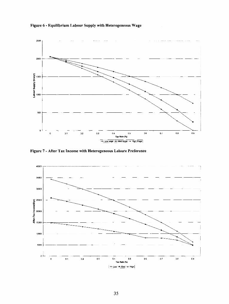
Figure 6 - Equilibrium Labour Supply with Heterogeneous Wage

0 0.1 0.2 0.3 0.4 05 06 0 7 0.8 0.Q

Tax Fate (Y.)

F r w wwage + Med Wage +High Wage 1

Figure 7 - After Tax Income with Heterogeneous Leisure Preference

0 0 1 0.2 0.3 0.4 0.5 0.6 0.7 0.8 0 9

Tax Fate (%)

LOW +Med + H I Q ~ ~

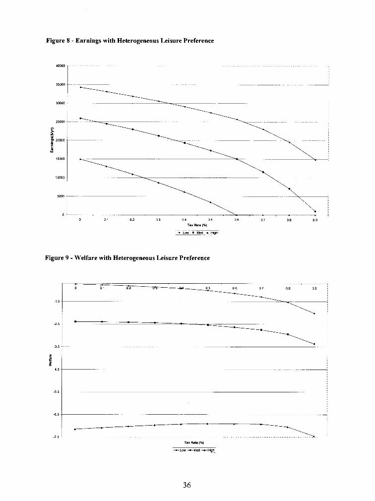
Figure 8 - Earnings with Heterogeneous Leisure Preference

Figure 9 - Welfare with Heterogeneous Leisure Preference

- 1 -&\ -7 3

Tax Rate (X)

I - t ~ o w +Med - t ~ l g h ]

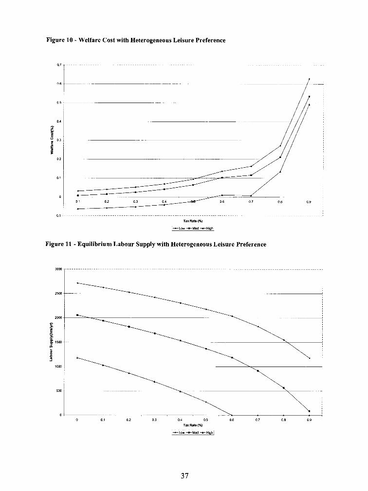
Figure 10 - Welfare Cost with Heterogeneous Leisure Preference

01

Tax Rate (Y.)

1-LOW + ~ e d HI^

Figure 11 - Equilibrium Labour Supply with Heterogeneous Leisure Preference

, - , - 0 0.1 0 2 0.3 0.4 0.5 0.6 0.7

Tax Rate (.A)

r--bw +Med +nigh 1

Figure 12 - After Tax Income with Hetergeneous Wage and Leisure Preference

0 0 1 0 2 0 3 0 4 0 5 0 6 0 7 0 8 0 9

Tax (%) - --

t ~ o w w , ~ o w ~ ~ ~ o w w , r n e d ~ t ~ o w w , h ~ g h ~ X r n e d w , l o w I X r n e d w , r n e d l t m e d w , h ~ g h ~ + h ~ g h w , ~ o w ~ - h ~ g h w , r n e d l - h ~ ~ h w , h ~ g h ~ ,

Figure 13 - Earnings with Heterogeneous Wage and Leisure Preference

-- Tax Rate (%)

L-w,!ow I +low w, rned I t low w, hlgh I X r n e d w, low I *med w, rned I t r n e d w, hlgh I thigh w, low I - - hlgh w, rned I - hlgh w, high I ~

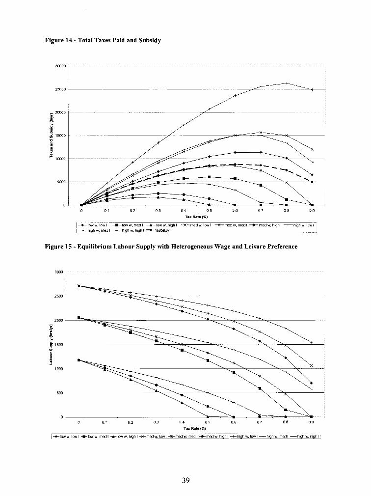
Figure 14 - Total Taxes Paid and Subsidy

0 0 1 0.2 0.3 0.4 0.5 0.6 0 7 0.8 0 9

Tax Rate (Ye)

I t l o w w, low l %low w, rned I +low w, high I X r n e d w, low I e r n e d w, rned I t r n e d w, high I 1- hlgh w, rned I -high w, high I + -subsidy

Figure 15 - Equilibrium Labour Supply with Heterogeneous Wage and Leisure Preference

0 0.1 0.2 0.3 0 4 0.5 0.6 0 7 0.8 0 9

Tax Rate (%)

It low w, low I +-low w, rned I -A- low w, high I -++ rned w, low I -E rned w, rned I t rned w, hlgh I t h i g h w, low I - hlgh w, rned I - hlgh w, high I

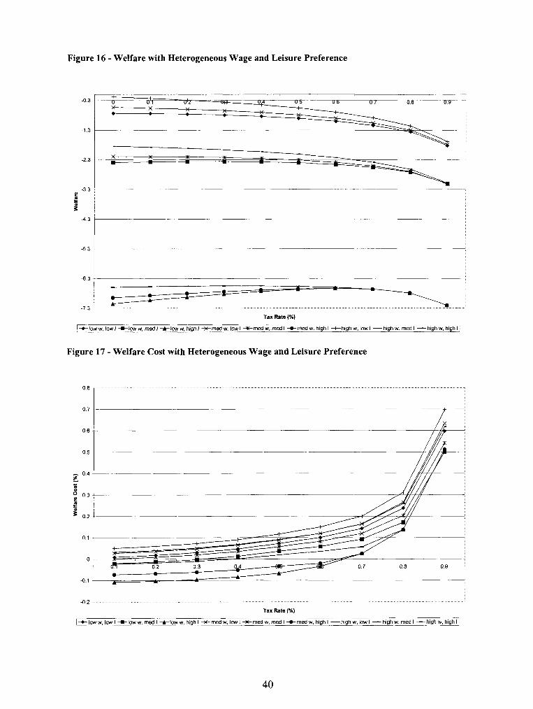
Figure 16 - Welfare with Heterogeneous Wage and Leisure Preference

Tax Rate (%) - . --

I-+~OWW,IOWI f loww,rnedI t l o w w , h i g h I Xrnedw, lOwI -Ytrned~,medI tmedw,h igh~+h lghw, low~-h lghw,medI -hlghw,highIj

Figure 17 - Welfare Cost with Heterogeneous Wage and Leisure Preference

Tax Rate (%) -

i+low w, low I +loww, med I +low w, high I X r n e d w, low I +med w, med I t m e d w, high I thigh w, low I -high w, med I -high w, high 1 1

Appendix B: Tables

Table 1 - Model Results with Heterogeneous Wage

Tax 1 After-tax income I Earnings 1 Welfare 1 Low I Medium I High Low I Medium I High I Low I Medium I High I

Tax

Table 2 - Model Results with Heterogeneous Leisure Preference

0

0.1

Labour Supply

Low I Medium I High

2055.096

1902.354

-

Tax

Welfare Costs

Low I Medium I High

Labour Supply Elasticity

Low I Medium I High

2055.096

1929.871

After-tax income

Low 1 Medium I Hioh

2055.096

1966.781

Earnings

Low I Medium I High

Welfare

Low I Medium 1 High

nil

-0.026

nil

-0.003

nil

0.029

0.000

-0.009

0.000

-0.007

0.000

-0.005

Table 3 - Model Results with Heterogeneous Wage and Preference for Leisure

After Tax Income

I I Low wape 1 Med waae I Hiah waae I

Earnings

Tax

0

Low L

28075.370

Tax

Med L

21255.858

Low wage

Low L I Med L I High L

High L

12219.551

Med wage

Low L I Med L I High L

High wage

Low L I Med L I High L

Low L

34264.275

Med L

25941.477

High L

14913.216

Low L

48650.765

Med L

36833.485

High L

21 174.806

Welfare

Eauilibrium Labour Supply

Low wape I Med wage

Tax

0

High wage

Low L

-0.733

Tax

Welfare Cost

Med L

-2.392

Low wage

Low L I Med L 1 High L

Low waae

Tax

0.1

High L

-7.148

Med wage

Low L I Med L I High L

Med wage

Low L

0.009

High wage

Low L I Med L I High L

High wage

Low L

-0.534

Med L

-0.021

Med L

-2.192

High L

-0.108

High L

-6.949

Low L

0.027

Low L

-0.183

Med L

0.001

MedL

-1.842

High L

-0.073

High L

-6.598

Low L

0.050

Med L

0.032

High L

-0.023

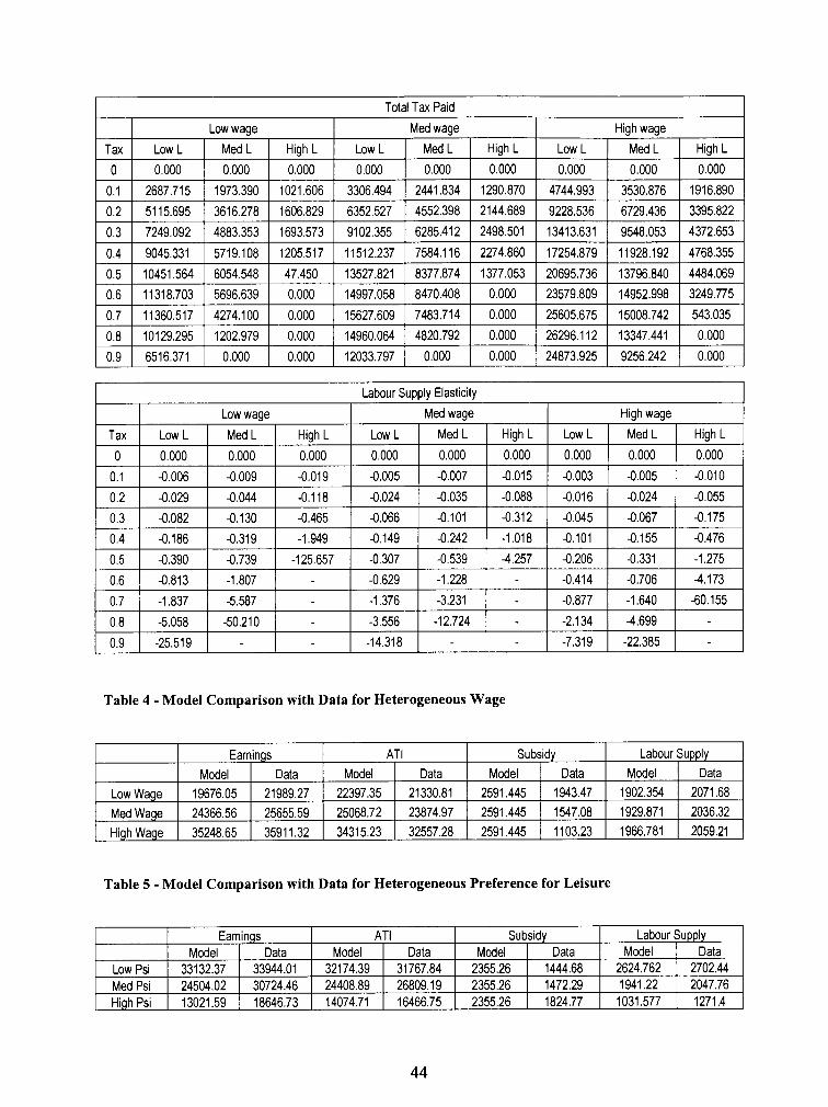
Total Tax Paid

I Low waae I Med waae I Hiah waae 1

Labour Supply Elasticity

Tax

0

Table 4 - Model Comparison with Data for Heterogeneous Wage

Tax

0

Table 5 - Model Comparison with Data for Heterogeneous Preference for Leisure

" "

High L

0.000

Low L

0.000

Low wage

" ., Med L

0.000

Low L

0.000

High L

0.000

Low L

0.000

Low L

0.000

Med wage

Med L

0.000

Low L

0.000

High wage

Med L

0.000

Med L

0.000

Low L

0.000

High L

0.000

High L

0.000

Med L

0.000

High L

0.000

Med L

0.000

High L

0.000

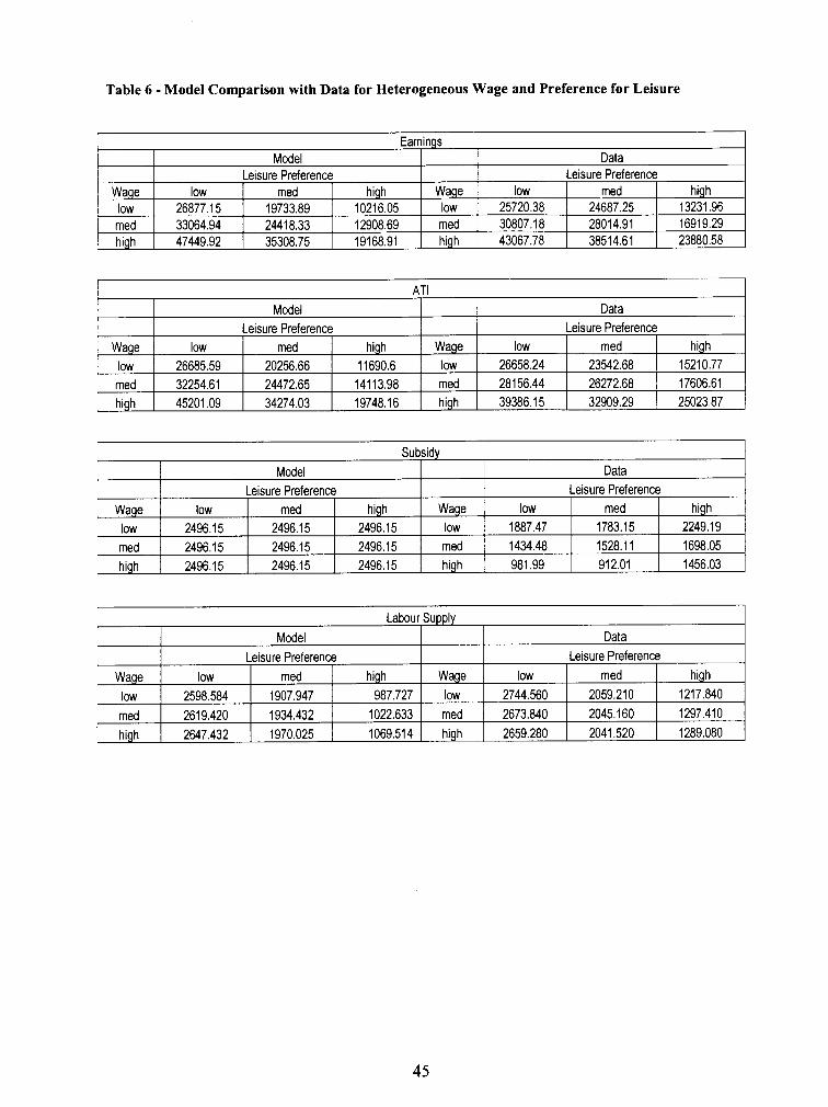
Table 6 - Model Comparison with Data for Heterogeneous Wage and Preference for Leisure

-

Earnings Model

Wage low rned high

Data

Subsidy

I high 1 2496.15 1 2496.15 1 2496.15 1 high I 981.99 912.01 1 1456.03 1

Model Leisure Preference

Wage low rned

Leisure Preference

Data Leisure Preference

Wage low rned high

low 26877.15 33064.94 47449.92

low 2496.15 2496.1 5

Leisure Preference med

19733.89 2441 8.33 35308.75

rned 2496.15 2496.15

low 25720.38 30807.18 43067.78

high 10216.05 12908.69 19168.91

high 2496.15 2496.15

rned 24687.25 28014.91 38514.61

high 13231.96 16919.29 23880.58

Wage low rned

low 1887.47 1434.48

rned 1783.15 1528.11

high 2249.19 1698.05

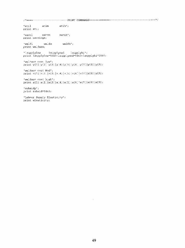
Appendix C: Gauss Code

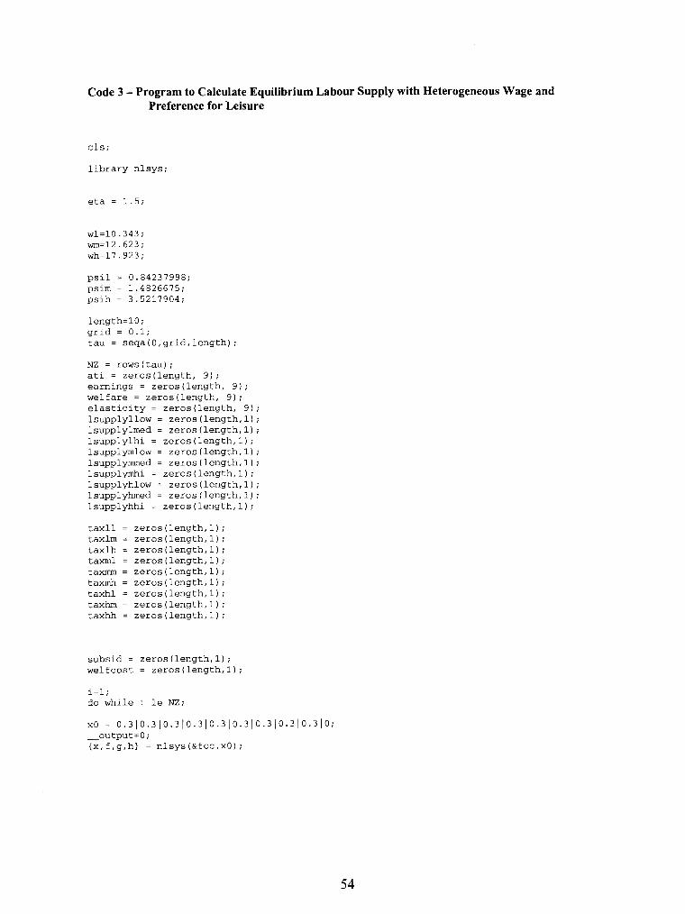
Code 1 - Program to Calculate Equilibrium Labour Supply with Heterogeneous Wage

cls;

library nlsys;

eta = 1.5;

length=lO; grid = 0.1; tao = seqa(o,grid,length);

NZ = rows(tao); ati = zeros(length, 3); earnings = zeros(length, 3); welfare = zeros(length, 3); lsupplylow = zeros(length,l); lsupplymed = zeros(length,l); lsupplyhi = zeros(length,l); subsid = zeros (length, 1) ; welfcost = zeros(length,l); elasticity = zeros(length, 3);

i=l; do while i le NZ;

earn1 = (wl*x[ll)*5840; earnm = (wm*x[21) *584O; earnh = (wh*x[31)*5840;

earnings[i, .I = earnl-earnm-earnh;

atil = (1-tao[i])*earnl + subsid[i]*5840; atim = (I-tao[i])*earnm + subsid[i]*5840; atih = (1-tao[il)*earnh + subsid[il*5840;

ati [i, . ] = atil-atim-atih;

welfl = In( (1-tao[i])*wl*x[l] + subsid[il) + (psi/(l-eta) ) * ( (1-x[l])^(l-eta)); welfm = ln((1-tao[i])*wm*x[2] + subsid[i]) + (psi/(l-eta))*((l-x[2I)Yl-eta)); welfh = ln((1-tao[i])*wh*x[3] + subsid[i]) + (psi/(l-eta) ) * ( (1-x[31 )"(I-eta));

welfare[i, .I = welfl-welfm-welfh;

fnl = ((1-tao[i] )*wl/ ((1-tao[i])*x[ll*wl + x[4l)) - psi*(l-~[ll) (-eta); fn2 = ((1-tao[i])*wm/( (1-tao[i])*x[2l*wm + x[41)) - psi*(l-x[21) A (beta); fn3 = ((1-tao[i])*wh/( (1-tao[il)*x[3l*wh + x[41)) - psi*(l-x[31) A (-eta); fn4 = (((tao[i]/4)*wl*x[l]) + ((tao[il/2)*wm*x[2]) + ((tao[il/4)*wh*x[31) 1 4 ;

if x[l] > 0 and x[21 > 0 and x[31 > 0; retp (fnllfn21fn31fn4); elseif x[l] le 0 and xi21 > 0 and x[31 > 0; retp (fn51fn61fn71fn8); endi f ; endp ;

fnl = (ln((l+y[l])*((l-tao[2])*wl*lsupplylow[21 + subsidL21)) + (psi/(l-eta))* ((1-lsupplylow[21)"(l-eta))) - welfare[l,ll; fn2 = (ln((l+y[2])*((l-tao[3])*wl*lsupplylow[31 + subsid[3])) + (psi/(l-eta))* ((1-lsupplylow[3])"(l-eta))) - welfare[2,11;

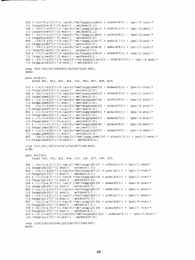
* ( (1-tao[4])*wl*lsupplylow[4] + subsid "(1-eta))) - welfareI3,ll; *((l-tao[5])*wl*lsupplylow[5] + subsid "(1-eta))) - welfare[4,11; * ( (1-tao[6])*wl*lsupplylow[6] + subsid "(1-eta) 1 ) - welfare[5,11; *((l-tao[7])*wl*lsupplylow[7] + subsid

retp (fnlJfn2)fn3)fn4)fn5lfn6] endp ;

proc foc2 ( z ; local fnl, fn2, fn3, fn4,

fnl = (In( (l+z [l]) * ((1-tao[2]) *wm*lsupplymed[2 + subsid[21)) + (psi/ (1-eta) ) * ((1-lsupplymed[2] )^(l-eta))) - welfare[l,21; fn2 = (In((l+z[2])*( (l-tao[3])*wm*1supplymed[31 + subsidL31)) + (psi/ (1-eta) ) * ((l-lsupplymed[31)A(l-eta))) - welfare[2,21;

((1-lsupplymed[lOl)"(l-eta))) - welfare[9,21;

retp (fnl)fn2)fn3)fn4)fn5)fn6)fn7)fn8)fn9); endp ;

proc foc3 (a) ; local fnl, fn2, fn3, fn4, fn5, fn6, fn7, fn8, fn9;

fnl = (In( (l+a[ll) * ((1-tao[2]) *wh*lsupplyhi[21 + subsid ((1-lsupplyhi[2l)"(l-eta))) - welfare[l,31; fn2 = (In( (l+a[2] ) * ( (1-tao[3] ) *wh*lsupplyhi [31 + subsid

((1-lsupplyhi[7])"(1-eta))) - welfare[6,31; fn7 = (In( (l+a[7])*((l-tao[8] )*wh*lsupplyhi[8] + subsid[8 ((1-lsupplyhi[8])"(1-eta))) - welfare[7,31; fn8 = (In( (l+a[8] ) * ( (1-tao[9]) *wh*lsupplyhi [91 + subsid19 ((l-ls~pplyhi[9])~(1-eta))) - welfare[8,31; fn9 = (In( (l+a[9] ) * ( (1-tao[lOl) *wh*lsupplyhi [lo] + subsid ((1-ls~pplyhi[lO])~(l-eta))) - welfare[9,3];

retp (fnl)fn2)fn3)fn41fn5Jfn61fn71fn81fn9); endp ;

"atil atim atih" ; print ati;

"earn1 earnm earnh" ; print earnings;

"welf 1 welfm welfh"; print welfare;

"Isupplylow lsupplymed lsupplyhi"; print lsupplylow*5840-lsupplymed*5840-lsupplyhi*5840;

"welfare cost low"; print ~ [ l l ly[21 ly[31 ly[41

" subsidy" ; print subsid*5840;

"Labour Supply Elasticity"; print elasticity;

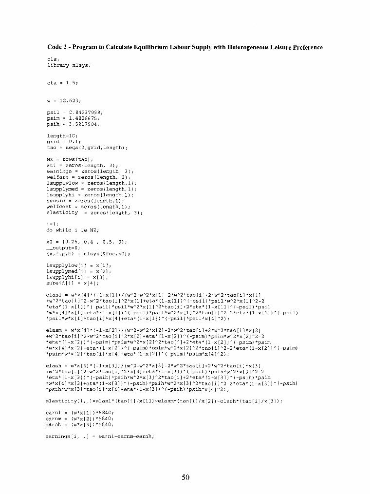
Code 2 - Program to Calculate Equilibrium Labour Supply with Heterogeneous Leisure Preference

cls; library nlsys;

eta = 1.5;

psi1 = 0.84237998; psim = 1.4826675; psih = 3.5217904;

length=lO; grid = 0.1; tao = seqa(O,grid,length);

NZ = rows(tao); ati = zeros(length, 3); earnings = zeros(length, 3); welfare = zeros(length, 3); Isupplylow = zeros(length,l); lsupplymed = zeros(length,l); lsupplyhi = zeros(length,l); subsid = zeros(length,l); welfcost = zeros(length,l); elasticity = zeros(length, 3);

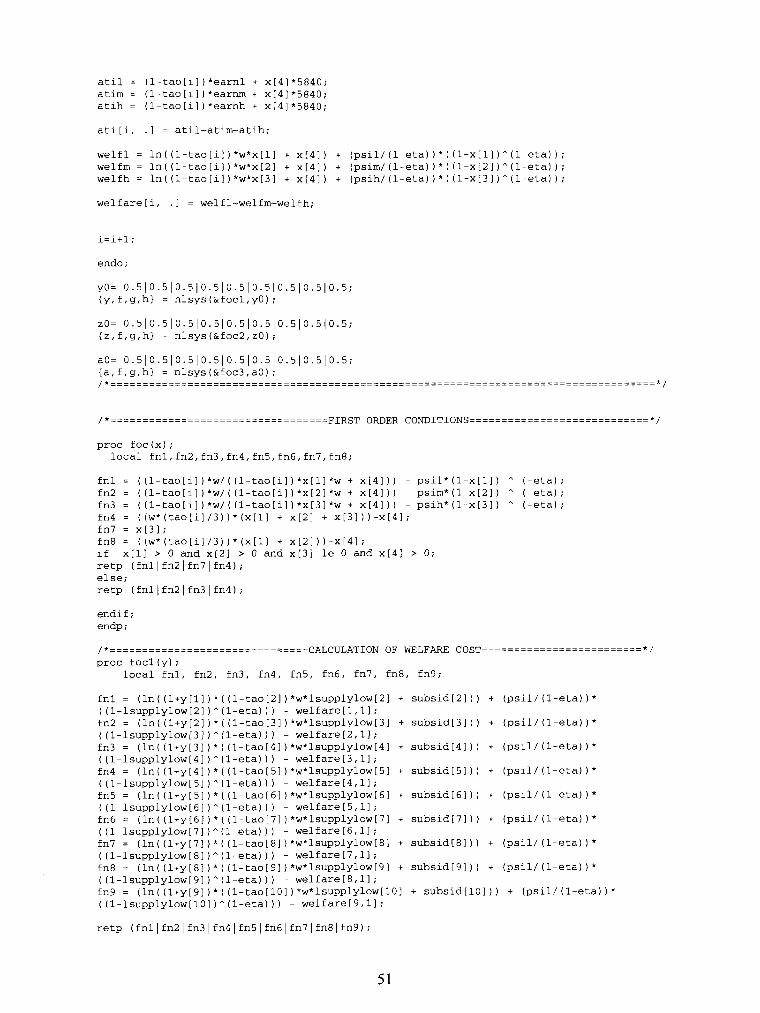
i=l; do while i le NZ;

elasm = w*x[4]*(-1+x[2])/(wA2-~A2*~[2]-2*~A2*tao[il+2*w*2*tao[il*x[2l +wA2*tao[i1A2-wA2*tao[i]^2*x[21+eta*(l-x[21)A~-psim)*psim*wA2*x[2]A2-2 *eta* (1-x[2] )A(-psim) *psim*w^2*x[21"2*tao[i]+2*eta*(l-x[2])A(-psim) *psim *w*x[4] *~[2]+eta*(l-x[2])*(-~sim) *p~im*w~2*~[2]*2*tao[i]~2-2*eta* (1-x[2] )*(-psim) *psim*w*x[2] *tao[i] *x[41 +eta* (1-x[21) "-psim) *psim*x[4] *2) ;

earn1 = (w*x[l] ) *584O; earnm = (w*x[21) *584O; earnh = (w*x[3] ) *584O;

earnings[i, .I = earnl-earnm-earnh;

atil = (1-tao[i])*earnl + x[4]*5840; atim = (1-taolil )*earnm + x[41*5840; atih = (1-tao[i] ) *earnh + x[4] *584O;

ati [i, . I = atil-atim-atih;

welfare[i, .I = welfl-welfm-welfh;

proc foc (x) ; local fnl,fn2,fn3,fn4,fn5,fn6,•’~17,fn8;

fnl = ((1-tao[i]) *w/ ((1-tao[il) *x[ll *w + x[41)) - psil*(l-x[ll ) ^ (-eta) ; fn2 = ((1-tao[i] )*w/((l-tao[i])*x[2l*w + x[41 ) ) - psim*(l-x[21) ̂ (-eta); fn3 = ((1-tao[i] )*w/((l-tao[il)*x[3l*w + x[41 ) ) - psih*(l-x[31) ̂ (-eta); fn4 = ( (w* (tao[i] /3)) * (x[ll + x[21 + x[31)) -x[41 ; fn7 = x[31; fn8 = ((w*(tao[i]/3))*(x[l] + x[2]))-x[41; if x[l] > 0 and x[2] > 0 and x[3] le 0 and x[4j > 0; retp (fnllfn21fn71fn4); else; retp (fnllfn21fn31fn4);

endi f ; endp ;

((1-lsupplylow[9])^(leta)))) fn9 = (In( (l+y[g])*( (1-tao[10 ( (1-lsupplylow[lOl )*eta) ) )

retp (fnllfn21fn31fn4jfn5lfn6

endp ;

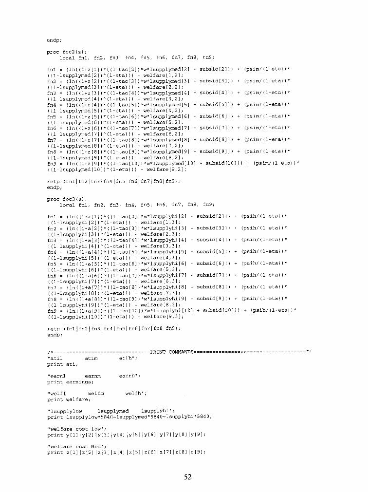
proc foc2(z); local fnl, fn2, fn3, fn4,

fnl = (ln((l+z[l] ) * ( (1-tao[2] ((1-lsupplymed[21)"(1-eta))) fn2 = (ln((l+z[2] ) * ( (1-tao[3]

retp (fnllfn2lfn3 endp ;

local fnl, fn2, fn3, fn4, fn5, fn6, fn

fnl = (ln((l+a[l])*((l-tao[2])*w*lsupplyhi ((1-lsupplyhi[2])"(1-eta))) - welfare[l,31 fn2 = (ln((l+a[2])*((l-tao[3])*w*lsupplyhi ((1-lsupplyhi[3])*(1-eta))) - welfare[2,31 fn3 = (ln((l+a[3])*( (1-tao[4])*w*lsupplyhi ((I-lsupplyhi[4])"(1-eta))) - welfareI3,31 fn4 = (ln((l+a[4])*((1-tao[5])*w*lsupplyhi

^(l-eta))) - welfare[4,31; ) * ( (1-tao[6] ) *w*lsupplyhi[61 + subsid[6 "(1-eta))) - welfare[5,31; ) * ((1-tao[7]) *w*lsupplyhi[71 + subsidL7 ^(I-eta))) - welfare[6,31; ) * ((1-tao[8]) *w*lsupplyhi[81 + subsid[8 *(l-eta))) - welfare[7,31; ) * ((1-tao[9]) *w*lsupplyhi[91 + subsid[9 A(l-eta))) - welfare[8,31; )*((l-tao[lO])*w*lsupplyhi[l01 + subsid

retp (fnllfn21fn31fn41fn5lfn61fn71fn81fn9); endp ;

" earn1 earnrn earnh" ; print earnings;

"welfl welfm welfh"; print welfare;

Ml~~pplylow lsupplymed lsupplyhi"; print lsupplylow*5840-lsupplymed*5840-lsupplyh*5840;

"welfare cost low"; print ~ [ l l ly[21 ly[31 1~141

"welfare cost Med"; print z[11 1z[21 1z[31 1z[41

"subsidy"; print subsid*5840;

"Labour Supply Elasticity"; print elasticity;

Code 3 - Program to Calculate Equilibrium Labour Supply with Heterogeneous Wage and Preference for Leisure

library nlsys;

eta = 1.5;

psi1 = 0.84237998; psim = 1.4826675; psih = 3.5217904;

length=lO; grid = 0.1; tau = seqa(O,grid,length);

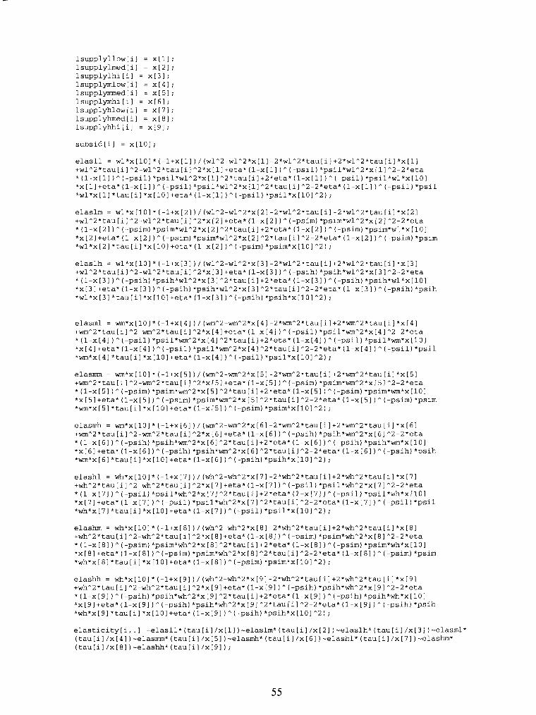
NZ = rows(tau); ati = zeros(length, 9) ; earnings = zeros(length, 9 welfare = zeros(length, 9) elasticity = zeros(length, lsupplyllow = zeros(1ength lsupplylmed = zeros(1ength lsupplylhi = zeros(length,l lsupplymlow = zeros (length, 1) ; lsupplynuned = zeros(length,l); lsupplymhi = zeros(length,l); lsupplyhlow = zeros(length,l); lsupplyhmed = zeros(length,l); lsupplyhhi = zeros(length,l);

tax11 = taxlm = taxlh = taxml = t a m = taxmh = taxhl = taxhm = taxhh =

zeros(length,l); zeros (length, 1) ; zeros(length,l); zeros (length, 1) ; zeros (length, 1 ) ; zeros(length,l); zeros(length,l); zeros(length,l); zeros(length,l);

subsid = zeros(length,l); welfcost = zeros(length,l);

i=l; do while i le NZ;

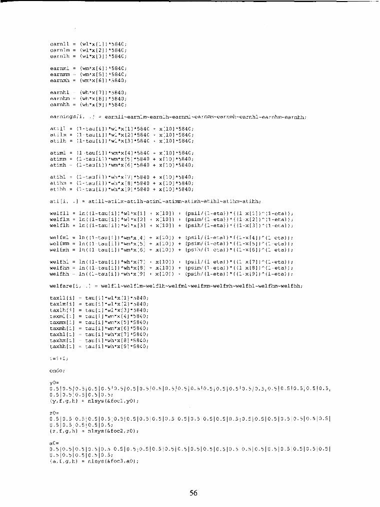
earn11 = (wl*x[ll ) *584O; earnlm = (wl*x[21 ) *584O; earnlh = (wl*x[31 ) *584O;

earnml = (wm*x[41 ) *584O; ear- = (wm*x[51 ) *584O; earnmh = (wm*x[61)*5840;

earnhl = (wh*x[7])*5840; earnhm = (wh*x[81)*5840; earnhh = (wh*x[9])*5840;

atill = (1-tau[il ) *wl*x[ll*5840 + x[101*5840; atilm = (1-tau[i] ) *wl*x[2] *584O + x[10] *584O; atilh = (1-tau[il)*wl*x[3]*5840 + x[101*5840;

atiml = (1-tau[il)*wm*x[4]*5840 + x[101*5840; atim = (1-tau[il ) *wm*x[5] *584O + x[101*5840; atimh = (1-tau[i] ) *wm*x[6] *584O + x[10] *584O;

atihl = (1-tau[i] ) *wh*x[7] *584O + x[101*5840; atihm = (1-tau[iI)*wh*x[81*5840 + x[101*5840; atihh = (1-tau[i])*wh*x[9]*5840 + x[101*5840;

ati[i, .I = a t i l l - a t i l m - a t i l h - a t i m l - a t i m - a t i h - a t i h h ;

welfll = In( (1-tau[i] )*wl*x[l] + x[10]) + (psil/ (1-eta)) * ((1-x[l] )"(l-eta) 1 ; welflm = In( (1-tau[i]) *wl*x[2] + x[101) + (psim/ (1-eta)) * ((1-x[2l )^(lets)); welflh = In( (1-tau[i])*wl*x[3] + x[10]) + (psih/ (1-eta) ) * ( (1-x[3] )%-eta) ) ;

welfhl = ln((1-tau[i])*wh*x[7] + x[10]) + (psill(1-eta))*((l-x[7] )"(I-eta) ) ;

welfhm = ln((1-tau[i])*wh*x[8] + x[10]) + (psim/(l-eta)) * ( (I-x[81 )"(I-eta) ) ;

welfhh = ln((1-tau[i])*wh*x[9] + ~1101) + (psih/(l-eta) )*((l-xl91 )^(I-eta));

welfare[i, .I = welfll-welflm-welflh-welfml-welfm-welfmh-welfhl-welfhm-welfhh;

zo= 0.5~0.5~0.5~0.5~0.5~0.5~0.5~0.5~0.5~0.5~0.5~0.5~0.5~0.5~0.5~0.5~0.5~0.5~0.5~0.5~0.5~0.5~ 0.510.510.510.510.5; {z, f,g,h) = nlsys(&foc2,zO);

aO= 0.5~0.5~0.5~0.5~0.5~0.5~0.5~0.5~0.5~0.5~0.5~0.5~0.5~0.5~0.5~0.5~0.5~0.5~0.5~0.5~0.5~~.5~ 0.510.510.510.510.5; {a, f,g,h} = nlsys(&foc3,aO) ;

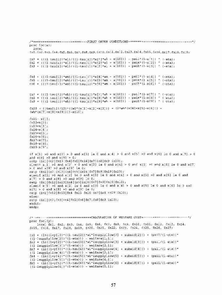
/*=============================FIRST ORDER CONDITIONS================================== * / proc foc(x); local

fnl,fn2,fn3,fn4,fn5,fn6,fn7,fn8,fn9,fn1O,fnll,f~~2,fn~~,f~~~,fnl5,fnl6,fnl7,fnl8,fnl9;

fnl = (((1-tau[i])*wl)/ ((1-tau[i])*x[l]*wl + x[101)) - psil*(l-x[l]) " (-eta) ; fn2 = (((1-tau[i])*wl)/((l-tau[i])*x[2]*wl + x[101)) - psim*(l-x[2]) * (-eta); fn3 = (((1-tau[i])*wl)/((l-tau[i])*x[3]*wl + x[101)) - psih*(l-x[31) " (-eta);

if x[l] >O and x[2] > 0 and x[3] le 0 and xi41 > 0 and x[51 >O and x[6] le 0 and x[7] > 0 and x[8] >O and x[91 > 0; retp (fnllfn2lfnl3lfn4lfn5Ifn16Ifn71fn8~fn9IfnlO); elseif x[l] >O and x[2] > 0 and x[3] le 0 and x[4] > 0 and x[51 >O and x[6] le 0 and x[71 > 0 and xi81 >O and x[91 le 0; retp (fnllfn2lfnl3lfn4lfn5Ifn16Ifn71fn8Ifn19IfnlO); elseif x[l] >O and x[2] le 0 and x[31 le 0 and x[41 > 0 and x[51 >O and x[61 le 0 and x[7] > 0 and x[8] >O and x[91 le 0; retp (fnl~fnl2~fnl3~fn4~fn5~fn16~fn71fn8~fn19~fnl0); elseif x[l] >O and x[2] le 0 and x[31 le 0 and x[41 > 0 and x[51 le 0 and xi61 le 0 and x[7] z 0 and x[8] >O and x[91 le 0; retp (fnllfnl2lfnl3lfn4lfnl5lfnl6lfn7lfn8lfnl9~fnl0); else; retp (fnllfn21fn31fn41fn5Ifn6lfn7)fn8lfn9IfnlO); endi f ; endp ;

/ *------------===----------------CALCULATION ------------ ---------------- O F WELFARE COST=========================*/

proc focl(y); local fnl, fn2, fn3, fn4, fn5, fn6, fn7, fn8, fn9, fnlO, fnll, fn12, fn13, •’1114,

fn15, fn16, •’1117, fn18, •’1119, •’1120, •’1121, •’1122, •’1123, •’1124, •’1125, fn26, fn27;

fnl = (In( (l+y[l] ) * ( (1-tau[2] ) *wl*lsupplyllow[21 + subsid[2] ) ) + (psil/ (1-eta) ) * ((1-lsupplyllow[2])^(1-eta))) - welfare[l,ll; fn2 = (ln((l+y[2])*((1-tau[3])*wl*lsupplyllow[3] + subsid[3])) + (psil/(l-eta))* ((1-lsupplyllow[3])*(l-eta))) - welfare[2,11; fn3 = (ln((l+y[3])*((l-tau[4])*wl*lsupplyllow[4] + subsid[4])) + (psil/(l-eta))* ((1-lsupplyllow[4]] "(1-eta))) - welfare[3,11; fn4 = (In( (l+y[4] ) * ( (1-tau[5] ) *wl*lsupplyllow[51 + subsid[5] ) ) + (psil/ (1-eta) ) * ((1-lsupplyllow[5])Yl-eta))) - welfare[4,11; fn5 = (ln((l+y[5])*((l-tau[6])*wl*ls~pplyllo~[61 + subsid[6])) + (psil/(l-eta))* ((1-lsupplyllow[6])"(l-eta))) - welfare[5,11;

)*wl*lsupplylmed[2] + subsid welfare[l,21; )*wl*lsupplylmed[3] + subsid welfare[2,21 ;

) *wl*lsupplylmed[4] + subsid welfare[3,21; )*wl*lsupplylmed[51 + subsid welfare[4,21; )*wl*lsupplylmed[61 + subsid

fnlO = (ln((l+y[lO ((1-lsupplylmed[2] fnll = (ln((l+y[ll ((1-lsupplylmed[3] •’1112 = (ln((l+y[12 ((1-lsupplylmed[4] •’1113 = (ln((l+y[13 ((1-lsupplylmed[5] •’1114 = (ln((l+y[14 ((1-lsupplylmed[6] fn15 = (ln((l+y[15 ((1-lsupplylrned[7] •’1116 = (ln( (l+y[l6 ((1-lsupplylmed[8] •’1117 = (ln((l+y[17 ((1-lsupplylmed[9] En18 = (ln( (l+y[l8 ((1-lsupplylmed[lO

endp ;

proc foc2 (z ) ; local fnl, fn2, fn3, fn4, fn5, fn6, fn7, fn8, fn9, fnlO, fnll, fn12

•’1120, •’1121, fn22, •’1123, •’1124, •’1125, •’1126,

fnl = (In( (l+z [l] ( (1-lsupplymlow[2 fn2 = (ln( (l+z[2] ((1-lsupplymlow[3 fn3 = (ln( (l+zI3] ( (1-lsupplymlow[4 fn4 = (ln((l+z[4] ((1-lsupplymlow[5 fn5 = (ln((l+z[5] ( (1-lsupplymlow[6 fn6 = (ln((l+z[6] ((1-lsupplymlow[7 'in7 = (ln( (l+z[7] ((l-lsupplymlow[8

eta) ) *

(1-eta) )

1-eta) )

1-eta) )

fnlO = (In( (l+z[lOl I * ( (1-tau12 ( (1-lsupplymmedl21) * (1-eta) ) ) fnll = (In( (l+z[lll) * ( (1-tau13 ((l-ls~pplymmed[31)~(l-eta))) fn12 = (In( (l+z[l21 ) * ( (1-tau14

*wm*lsupplymmed121 + subsid121 welfarell, 51; )*wm*lsupplymmed[31 + subsid131 welfare[2.51 ;

41 + subsid

51 + subsid

61 + subsid

71 + subsid

81 + subsid ((1-lsupplymhi[8l)^(l-eta))) - welfare[7,61; fn26 = (ln( (l+z[26] ) * ( (1-tau191) *wm*lsupplymhiI91 + subsidf91 ((1-lsupplymhi[9] )^(l-eta))) - welfare[8,61 ; fn27 = (ln( (l+z [27] ) * ( (1-tau[lOl) *wm*lsupplymhi 0 + subsidl ((1-lsupplymhi[lO])*(l-eta))) - welfarel9,61;

endp;

proc foc3 (a) ; local fnl, fn2, fn3, fn4,

•’1115, fn16, •’1117, •’1118, •’1119,

fnl = (In( (l+a[ll ) * ( (1-tau121 ((1-lsupplyhlow121 )Yl-eta))) fn2 = (In( (l+a[21 ) * ( (1-tau131 ((l-lsupplyhlow131)A(l-eta))) fn3 = (In( (l+a[31 )*((l-tau141 ((1-lsupplyhlowl4l)^(l-eta))) fn4 = (In( (l+a[41) * ((1-tau[5] ((1-lsupplyhlow[51 )*(l-eta))) fn5 = (In( (l+al5l) * ((1-tau161 ((l-ls~pplyhlow[61)~(l-eta) 1 ) fn6 = (In( (l+a[61 ) * ( (1-tau171 ((1-lsupplyhlow171)A(l-eta)))

retp (fnl~fn2~fn3~fn4~fn5~fn6~fn7~fn8~fn9~fnlO~fnll~fnl2~fnl3~fnl4~fnl5~fnl6~fnl7~fnl8~fnl9~ fn201fn211fn221fn231fn241fn251fn261fn27); endp ;

" earn1 earnm earnh" ; print earnings;

"welfl welfm welfh"; print welfare;

"Isupplyllow lsupplylmed lsupplylhi"; print lsupplyllow*5840-lsupplylmed*5840-lsupplylhi*584O;

ulsupplyrnlow lsupplynuned lsupplymhi"; print lsupplymlow*5840-lsupplymmed*5840-lsuppli*5840;

~lsupplyhlow lsupplyhmed lsupplyhhi"; print lsupplyhlow*5840-lsupplyhmed*584O-lsupplyhhi*5840;

"welfare cost low Med"; print ~[lol ly[llI ly[l21 ly[131 ly[141 ly[151 ly[161 ly[171 ly1181;

"welfare cost low high"; print y[191 1~[201 ly[211 ly[221 ly[231 1 ~ ~ 2 4 1 ly[251 1~1261 1 ~ 1 2 7 1 ;

"welfare cost med Med"; print z[101 1z[111 1z[121

"welfare cost med high" print z[191 1z[201 1z[211

"welfare cost hi low":

"welfare cost hi Med"; print a[lOl la[lll la[l21 la[131

"welfare cost hi high"; print a[191 la[201 la[211 lac221

"subsidy" ; print subsid*5840;

"taxes" ; print t a x l l - t a x l m - t a x l h - t a m l - t a m - t a x h ;

"Labour Supply Elasticity"; print elasticity;

BIBLIOGRAPHY

Andolfatto, David, Chns Ferrall and Paul Gomme. "Lifecycle Learning, Earning, Income and Wealth." Manuscript: Simon Fraser University (2000).

Andolfatto, David, and James Redekop. "Redistribution Policy in a Model with Heterogeneous Time-Preference." Manuscript: Simon Fraser University (2001).

Benjamin, Dwayne, and Morley Gunderson and W. Craig Riddell. Labour Market Economics: Theory, Evidence and Policy in Canada. 5th ed. Toronto: McGraw- Hill Ryerson Limited, 2002.

Government of Canada. Improving Social Security in Canada, Guaranteed Annual Income: A Supplementary Paper. Ottawa, 1 994.

Hum, Derek, and Wayne Simpson. "A Guaranteed Annual Income? From Mincome to the New Millenium." Policy Options (2001): 78-82.

Income Tax Rates and Personal Tax Credits[online] . Taxtips.ca, 12 April 2004 [cited 12 April 20041. Available from: <http://www.taxtips.ca~tax_rates.htm#FederalTaxRates>.

Murphy, Kevin M., and Finis Welch. "The Structure of Wages." The Quarterly Journal ofEconomics, no. 107 (1992): 285-326.

Neil, John R. "The Political Viability of a Negative Income Tax." Social Choice and Welfare, no. 18 (2000): 747-757.