An Exact Approach toHead-On Collisions of Black Holes

Fabian Muller

Master Thesis(30 HP/CP)

Fysikum

Supervisor:Prof. Dr.Kjell Rosquist

Institut furtheoretische Physik

Supervisor:Prof. Dr.

Luciano Rezzolla

November 25, 2014

Abstract

This work deals with head-on collisions of black holes in the full framework ofgeneral relativity. Starting with an overview on basic features of black holeswe proceed with applying concepts of the ADM formalism to set up spatialmetrics containing black holes of equal and unequal mass. Central to ourdiscussion will be the Weyl curvature of these metrics. Along curves thatare locally rotationally symmetric exact evolution equations for the Weylcurvature allow us to compute the time it takes for freely falling observersto fall in any one of the black holes. Additionally we are able to estimatea measure of collision time for freely falling black holes in a fully dynamicscenario.

”Our hopes and expectations,black holes and revelations.”

— Muse

Contents

1 Introduction 31.1 The History of Black Hole Research . . . . . . . . . . . . . . . 31.2 Motivation for this Work . . . . . . . . . . . . . . . . . . . . . 4

2 Black Holes in General Relativity 62.1 The Curvature of Spacetime . . . . . . . . . . . . . . . . . . . 62.2 The Schwarzschild Solution . . . . . . . . . . . . . . . . . . . 82.3 Isotropic Coordinates . . . . . . . . . . . . . . . . . . . . . . . 112.4 Infall Time . . . . . . . . . . . . . . . . . . . . . . . . . . . . 132.5 Interaction Energy of Two Black Holes . . . . . . . . . . . . . 152.6 The Area Theorem . . . . . . . . . . . . . . . . . . . . . . . . 16

3 Initial Data 183.1 Decomposition of Space and Time . . . . . . . . . . . . . . . . 183.2 Constraint Equations . . . . . . . . . . . . . . . . . . . . . . . 203.3 Conformal Flatness . . . . . . . . . . . . . . . . . . . . . . . . 213.4 Orthonormal Frame Approach . . . . . . . . . . . . . . . . . . 24

4 The LRS Concept 264.1 Choosing appropriate Coordinates . . . . . . . . . . . . . . . . 264.2 Evolution Equations . . . . . . . . . . . . . . . . . . . . . . . 28

5 Results 305.1 The Algorithm . . . . . . . . . . . . . . . . . . . . . . . . . . 305.2 Single Black Hole Solutions . . . . . . . . . . . . . . . . . . . 30

5.2.1 Weyl Curvature . . . . . . . . . . . . . . . . . . . . . . 305.2.2 Infall Times . . . . . . . . . . . . . . . . . . . . . . . . 32

5.3 Double Black Hole Solutions with Equal Masses . . . . . . . . 335.3.1 Weyl Curvature . . . . . . . . . . . . . . . . . . . . . . 335.3.2 Variation of Separation . . . . . . . . . . . . . . . . . . 355.3.3 Infall Times . . . . . . . . . . . . . . . . . . . . . . . . 37

5.4 Double Black Hole Solutions with Unequal Masses . . . . . . . 395.4.1 Infall Times . . . . . . . . . . . . . . . . . . . . . . . . 39

6 Conclusion 42

2

1 Introduction

1.1 The History of Black Hole Research

The first ideas of massive objects, from which not even light can escape, dateback to thought experiments of John Michell [1] and Pierre-Simon Laplace[2] in the late 18th century. However, it was not before the establishmentof general relativity by Albert Einstein that those objects appeared in aphysically consistent theory. Only months after Einstein’s publications KarlSchwarzschild derived what is now known as the Schwarzschild solution [3].Though generalizations to electrically charged black holes1 were formulatedby Hans Reissner [4] and Gunnar Nordstrom [5], the understanding of gravi-tational singularities posed significant challenges to the scientific community.Due to the lack of observational evidence development on this field remainedslow in subsequent decades. Black holes were only considered as hypotheti-cal end points of stellar evolution, when massive stars undergo gravitationalcollapse [6]. Since many physicists have been employed in the field of nuclearphysics during World War II and its aftermath, the dawn of the golden age ofgeneral relativity was postponed to occur half a century after Einstein pro-posed his theory. Especially the discovery of the first pulsar by Jocelyn BellBurnell and Antony Hewish [7] in 1967 convinced many scientists that com-pact objects, and thus black holes, might be more than just mathematicalcuriosities. Also around this time solutions to the Einstein Field Equationsfor (electrically charged) rotating black holes have been found by Roy Kerrand Ezra T. Newman [8, 9, 10]. Additionally the observational data of X-raybinary stars, backing up the existence of astrophysical black holes [11], es-tablished the branch of black hole physics in the scientific mainstream. The1970’s were marked by the advent of black hole thermodynamics [12] cul-minating in Stephen W. Hawking’s proposal that black holes emit thermalradiation [13]. With this particle creation process being a quantum mechan-ical effect in strong gravitational fields, theories of quantum gravity becamemore and more prominent. Black holes have always played a crucial role inthis context, since they represent one of the few domains, where quantum me-chanics and general relativity have to be combined. Eventually these trendsled Leonard Susskind to formulate the holographic principle [14] during the

1The term black hole was not used prior to the 1960’s.

3

second superstring revolution in 1995, which could describe higher dimen-sional black holes as a projection on their event horizons. This yet unprovenbut widely accepted conjecture has been proposed to resolve the informationparadox, which had been raised by Hawking’s radiation mechanism. Relatedideas of black holes being ensembles of stringy objects emerged from JuanMaldacena’s work [15]. Apart from those highly theoretical approaches theobservational search for astrophysical black holes has not stood still. Sincethe 1990’s it is commonly believed that supermassive black holes reside inthe centers of most (if not all) galaxies [16] and play a crucial role in theirevolution. The observation of stars orbiting the central region of our owngalaxy rules out the presence of every known astrophysical object with theexception of a black hole [17]. Over the last two decades some attention hasbeen drawn to the production of microscopic black holes in particle accelera-tors like the Large Hadron Collider (LHC) [18, 19]. However, no events havebeen recorded to this date imposing stricter boundary conditions on theorieswith large extra dimensions. While the search for primordial black holes con-tinues with the Fermi Gamma-ray Space Telescope, much effort is also putinto the detection of gravitational waves. The existence of these waves hasbeen confirmed indirectly with the observation of the Hulse-Taylor binarypulsar [20]. It is commonly believed that the collision of two black holes isamong the most intensive sources of gravitational waves. Early successes ofnumerical relativity obtained by Peter Anninos et al. provide estimates ofwave forms and energy scales of such gravitational radiation [21, 22, 23, 24].High precision in this field is necessary if one hopes to find congruent datain detection facilities like the Laser Interferometer Gravitational-Wave Ob-servatory (LIGO). Despite all of these promising projects a whole centuryof research has not been enough to gain a complete understanding of blackholes due to the lack of a consistent theory of quantum gravity.

1.2 Motivation for this Work

Solitary black holes have been studied extensively and many of their proper-ties can be extracted from Einstein’s theory of gravity analytically. Scenar-ios involving dynamical processes of interacting black holes are considerablymore difficult to investigate. This is mainly, because the exact solutionsto the Einstein field equations (EFE) are not known, so that physicists areforced to work with weak field approximations or numerical methods. These

4

are naturally accompanied by uncertainties, so that exact conclusions aboutgravitational wave generation and black hole mergers have eluded the re-searchers ever since. In fact it is believed that black hole collisions are amongthe most efficient sources of such radiation due to the high acceleration oflarge masses. However, the energy levels on which these effects occur cannot be given without inaccuracy. Furthermore such numerical estimates giveno particular insight into the spacetime geometry of metrics with more thanone black hole. Recently it was shown by Clifton et al. [25] how the Weylcurvature can be tracked throughout its entire evolution history along spe-cific curves of symmetry (cf. section 4) not approximately, but exactly. Sincethis method is applicable to spacetime metrics with an arbitrary number ofblack holes, we are confident to gain more knowledge about the dynamics ofcolliding black holes.

5

2 Black Holes in General Relativity

2.1 The Curvature of Spacetime

Most physical theories including special relativity have been formulated ina background of flat space in which proper distances ds between two eventsat (x, y) and (x + dx, y + dy) can straightforwardly be calculated with thePythagorean theorem (cf. Figure 1)

(ds)2 = (dx)2 + (dy)2 . (2.1)

The two-dimensional scenario depicted here can unambiguously be general-ized to the four-dimensional spacetime2

ds2 = −dt2 + dx2 + dy2 + dz2

= ηabdxadxb, (2.2)

where we have now introduced the symmetric matrix ηab = diag(−1, 1, 1, 1)and used the Einstein summation convention3 in the last line. The matrixηab is also called Minkowski metric, which is obviously only a subset of a moregeneral metric gab(x

a) that is curved in all four dimensions. Its components

2By convention the brackets around the differentials are omitted.3See appendix A for a detailed explanation regarding the notation.

Figure 1: In two-dimensional flat space the proper distance between twoevents at (x, y) and (x + dx, y + dy) is calculated with the Pythagoreantheorem.

6

can be coordinate-dependent and in general the off-diagonal entries are non-vanishing. Consequently invariant intervals in such a spacetime are measuredby the line element

ds2 = gabdxadxb. (2.3)

How far the given spacetime deviates from flat Minkowski spacetime can becalculated with the Riemann curvature tensor

Rabcd = ∂cΓ

abd − ∂dΓabc + ΓaecΓ

ebd − ΓaedΓ

ebc, (2.4)

where ∂a ≡ ∂∂xa

and the

Γabc =1

2gab (∂cgdb + ∂bgdc − ∂dgbc) (2.5)

are called Christoffel symbols4. The trace-free part of the Riemann tensor iscommonly referred to as the Weyl conformal tensor given in four dimensionsby

Cabcd = Rabcd −1

2(gacRbd − gadRbc − gbcRad + gbdRac)

+1

6(gacgbd − gadgbc)R. (2.6)

Here we encounter the contractions of the Riemann tensor that are (in ab-stract index notation) Rab = Rc

acb and R = Raa. These are known as the

Ricci tensor and the Ricci scalar respectively. Einstein’s realization hadbeen that the curvature of spacetime is directly related to the (local) energyand matter content Tab of the universe, thus giving rise to the Einstein fieldequations5 (EFE) [28]:

Rab −1

2gabR = 8πTab (2.7)

4in Eq.(2.5) gab denotes the inverse of the metric tensor gab.5A possible term with a cosmological constant has been omitted.

7

2.2 The Schwarzschild Solution

In this chapter we will develop the mathematical foundation of classical blackholes that are eventually a solution to Eq.(2.7). Up to this date the EFE canonly be solved exactly with the assumption of simplifying symmetry condi-tions. Apart from the completely flat Minkowski space the easiest scenariois that of a perfectly spherical mass, which is static and stationary. Math-ematically speaking the metric components of the desired line element ds2

are time-independent so that there do not appear any mixed terms dx0dxi.The spherical symmetry eliminates all mixed terms dxidxj for i 6= j. Withthis we can conclude that the line element must be of the form

ds2 = −A(r)dt2 +B(r)dr2 + C(r)r2dΩ2, (2.8)

with dΩ2 = dθ2 + sin2 θ dφ2. The line element Eq.(2.8) can be simplifiedfurther with the transformation Cr2 = r2 so that

dr

dr=√C

(1 +

r

2C

dC

dr

)and (2.9)

Bdr2 =B

C

(1 +

r

2CdCdr

)−2

dr ≡ Bdr. (2.10)

Together with A(r) = A(r) only two instead of three functions appear in theline element, which we write conventionally as

A(r) = e2ν(r) and B(r) = e2λ(r). (2.11)

Dropping the hats the new line element reads

ds2 = −e2νdt2 + e2λdr2 + r2dΩ2. (2.12)

The remaining task is to find the two yet unknown functions ν and λ. To dothat we have to solve the Einstein field equations (2.7), which in the absenceof matter reduce to the vacuum field equations :

Rab = 0 (2.13)

8

Three equations resulting from Eq.(2.12) and (2.13) are [29]

R00 =

(ν ′′ + ν ′2 − ν ′λ′ + 2ν ′

r

)e2ν−2λ = 0, (2.14)

R11 = −ν ′′ − ν ′2 + ν ′λ′ +2λ′

r= 0, (2.15)

R22 =(− 1− rν ′ + rλ′

)e−2λ + 1 = 0. (2.16)

Here the primes denote derivatives with respect to r. Since the exponentialfunction in Eq.(2.14) cannot become zero, we can sum it up together withEq.(2.15) to obtain ν ′ + λ′ = 0, which gives on integration

ν(r) = −λ(r). (2.17)

The integration constant that would appear is zero due to the boundarycondition of asymptotically flat space, i.e.

limr→∞

ν(r) = 0 = limr→∞

λ(r). (2.18)

With Eq.(2.17) we can integrate Eq.(2.16) to obtain after rearranging

e2ν = 1− 2M

r= −g00 = g−1

11 . (2.19)

The quantity 2M is a constant of integration chosen so that M turns out tobe the mass of the gravitating body, when the comparison with the weak fieldapproximation is done. Eventually we are able to write down the desired lineelement in its original form

ds2 = −(

1− 2M

R

)dt2 +

(1− 2M

R

)−1

dR2 +R2dΩ2, (2.20)

which is called the Schwarzschild solution6. In the following we want to pointout some of the most important features of this metric:

(i)Vacuum Solution: Recalling the derivation above we must note that theSchwarzschild metric approaches Minkowski spacetime ηab at infinitymeaning that there is no mass or energy inside the system except thebody with mass M .

6To properly distinguish the Schwarzschild coordinates from the isotropic coordinates(cf. section 2.3) we changed the notation from r to R .

9

(ii) Event Horizon: It can be seen easily from g11 that the metric shows adiverging behaviour when approaching R = 2M ≡ RS, which is calledthe gravitational or Schwarzschild radius. When crossing RS, the sig-nature of the metric changes, i.e. timelike components becoming space-like and vice versa. Thus, apparently the Schwarzschild coordinates losetheir validity for R ≤ RS. However, it can be shown that the divergenceat RS is a result of bad coordinate choice, so that we speak about acoordinate singularity. There exist various coordinate transformations(e.g Eq.(2.26)) that can resolve the singularity. On the other hand theSchwarzschild radius gives rise to more perplexing features that cannotso straightforwardly be seen from the metric (2.20). For example, RS

coincides with the surface from which not even light can escape. Thisfeature eventually corresponds to the term black hole, since everythingdisappears behind something that is called event horizon. The conceptof such horizons working as a one-way membrane [30] ”still continuesto confuse physicists today”7.

(iii) Gravitational Singularity: It is interesting to consider that M is nota function of R, which means that the spacetime generated outside ofthe massive body is independent of the mass distribution. Like in New-tonian gravity it is of no relevance, if the mass is evenly distributedin spherical shells or concentrated in a singular point. In fact in theabsence of any opposing force8 all matter is falling to the central point.Though we cannot make any conclusion about this point from the met-ric directly (cf.(ii)), we are still able to compute the Kretschmann scalar

RabcdRabcd = 48

M2

R6, (2.21)

which is perfectly regular for R = RS but is diverging for R→ 0. Thisbehaviour is called gravitational or curvature singularity. The simul-taneous occurrence of the different types of singularities led Penroseto his cosmic censorship hypothesis, which states that every physicalsingularity must be hidden from the outside world by an event horizon.As we are approaching a domain of spacetime and matter that shouldbe governed by (still unknown) quantum gravity effects, this feature is

7This was a remark by Herman Verlinde at the Karl-Schwarzschild-Meeting in 2013.8“Regular” stars are prevented from collapse due to radiative and degeneracy pressure.

10

believed by many physicists to indicate the breakdown of the theory ofgeneral relativity.

(iv) Birkhoff’s Theorem: There exist generalizations of the Schwarzschildsolution including charge Q (Reissner-Nordstrom metric), angular mo-mentum J (Kerr metric) or both (Kerr-Newman metric) all reduc-ing to Eq.(2.20) in the limit of Q, J → 0. Furthermore it can beshown [29] that any spherically symmetric vacuum solution must bea Schwarzschild solution, even if A,B and C in Eq.(2.8) are time-dependent. This is known as Birkhoff’s theorem.

We may conclude this section with the realization that the Schwarzschildsolution is the most important spacetime metric in black hole physics (if notin general relativity) and it will be the basis for all subsequent developmentsof this work.

2.3 Isotropic Coordinates

We have already mentioned that Schwarzschild coordinates may not neces-sarily be the best way to handle black hole solutions due to the appearanceof coordinate singularities. One set of coordinates that resolves this prob-lem (at least for the spatial part) is the isotropic metrical system, which isgenerally defined for a spherical configuration by

ds2 = −α2(r)dt2 + ψ4(r)(dr2 + r2

(dθ2 + sin θ2dφ

)). (2.22)

The functions α and ψ are yet to be determined functions of the isotropic ra-dial coordinate r, while the power of four is an arbitrary choice that will turnout to be practical, but has no deeper motivation. To find the correspondingtransformation between the Schwarzschild and the isotropic coordinates, it issufficient to concentrate on the spatial part of the metric only. With settingR = f(r) and consequently dR = f ′(r)dr we can write(

1− 2M

R

)−1

dR2 +R2dΩ2 =f ′2(r)

1− 2Mf(r)

dr2 + f 2(r)dΩ2

≡ ψ4(r)(dr2 + r2dΩ2

), (2.23)

11

which leads to the set of differential equations:

f ′2(r) = ψ4(r)

(1− 2M

f(r)

)(2.24)

f 2(r) = ψ4(r)r2 (2.25)

The solution to this is given by

R = f(r) = r

(1 +

M

2r

)2

(2.26)

and ψ =

(1 +

M

2r

). (2.27)

With the transformation (2.26) the Schwarzschild metric (2.20) can be writ-ten in isotropic form as:

ds2 = −(1− M

2r

)2(1 + M

2r

)2 dt2 +

(1 +

M

2r

)4(dr2 + r2dΩ2

)(2.28)

Still this metric is ill-defined for the point r = M/2, because the timelikecomponent vanishes and the metric becomes entirely spatial. However, if

Figure 2: This two-dimensional projection of the spatial part of the isotropicmetric (cf. Eq.(2.28) shows how two isomorphic spaces, 0 ≤ r ≤ M/2 andM/2 ≤ r ≤ ∞, are connected at the throat r = M/2. This is often referredto as an Einstein-Rosen bridge. The figure is taken from [30].

12

we concentrate on the spatial part of Eq.(2.28), we no longer encounter anycoordinate singularity. While the point R = 0 in the Schwarzschild repre-sentation refers to the position of the curvature singularity, the point r = 0in the isotropic formulation is isomorphically mapped to spatial infinity [30],which can also be shown by the following transformation:

r =

(M

2

)21

r. (2.29)

This property is illustrated by Figure 2 and one can understand it as twoidentical spaces being connected at the gravitational radius r = M/2, whichis often termed the black hole throat or an Einstein-Rosen bridge. We willsometimes refer to the metrical part 0 ≤ r ≤M/2 as the “parallel universe”.Lastly we want to emphasize that the isotropic coordinates, much like theSchwarzschild coordinates, only cover the exterior part of the black holemetric.

2.4 Infall Time

In the following we will now investigate the infall of particles into a blackhole. We are especially interested in the time a particle takes to hit thesingularity at R = 0 when falling from a finite distance R0. Due to the highdegree of symmetry of the Schwarzschild solution we can limit the discussionto radial trajectories. Considering null curves for which ds2 = 0 the metric(2.20) becomes

−(

1− 2M

R

)dt2 +

(1− 2M

R

)−1

dR2 = 0. (2.30)

It follows that

dt

dR= ±

(1− 2M

R

)−1

, (2.31)

which gives on integration

t− t0 ∼ ln(R−RS

)R→RS→ ∞. (2.32)

13

Apparently the distant observer would never see the particle hitting the blackhole singularity, because it takes an infinite amount of time to reach theevent horizon RS. As indicated in section 2.2 this feature is a result ofbad coordinate choices. If we try to calculate the infall time in a comovingreference frame, we will eventually see that the particle crosses the eventhorizon smoothly. To do that we employ the variational principle [31]

δ

∫ [−(

1− 2M

R

)t2 +

(1− 2M

R

)−1

R2︸ ︷︷ ︸≡I

]dτ = 0 (2.33)

and solve the Euler-Lagrange equations

d

dτ

∂I

∂xσ− ∂I

∂xσ= 0 (2.34)

to find for x0 = t:

d

dτ

[− 2

(1− 2M

R

)t

]= 0 =⇒

(1− 2M

R

)t = γ (2.35)

Here the overdots denote derivatives with respect to the proper time τ andγ is simply a constant of integration. For timelike curves we can write

−(

1− 2M

R

)t2 +

(1− 2M

R

)−1

R2 = −1 (2.36)

so that we obtain with Eq.(2.35)

R2 = γ2 −(

1− 2M

R

). (2.37)

To know what γ is, we have to impose the boundary condition that theparticle is initially at rest starting from R = R0, i.e. R2(R = R0) = 0. Thestraightforward result is

γ = ±√

1− 2M

R0

. (2.38)

It is noteworthy that for γ in order to be a real quantity the starting point R0

has to be outside the gravitational radius RS = 2M . Equivalently inside the

14

event horizon the stationary condition cannot be fulfilled so that no particlecan ever be at rest and must fall to the singularity. Proceeding with theseparation of variables yields

τ − τ0 = ±∫ R0

0

dR1√

RS

R− RS

R0

, (2.39)

where the integral can be written in parametric form [32] as:

R =R0

2

(1 + cos η

)(2.40)

τ =R0

2

(R0

2M

)1/2(η + sin η

)(2.41)

Here τ0 has been set to zero. The total proper time to reach the center ofthe black hole at R = 0 is given by η = π with

τ =π

2R0

(R0

2M

)1/2

. (2.42)

Obviously the diverging behaviour of the impact time found in Eq.(2.32) doesnot appear any more. In fact nothing particular happens at the Schwarzschildradius RS = 2M .

2.5 Interaction Energy of Two Black Holes

So far we have only considered the properties of single black holes. Whilewe will leave the discussion about metrics with more than one black hole tochapter 3, we will now investigate how two black holes interact energetically.It is intuitive to conclude that a system constituted of multiple black holesdoes not only contain the holes’ masses mi, which we will from here on callproper or bare masses, but also the energy that is attributed to the holes’ in-teraction. Thus, we cannot straightforwardly sum up multiple Schwarzschildsolutions, since the mass parameter M appearing in the Schwarzschild met-ric (cf. Eq.(2.20)) would require a new physical interpretation. A relationbetween the mass parameters Mi and the bare masses mi for scenarios withmultiple black holes was given by Brill and Lindquist [33] with

mi = Mi +∑j 6=i

MiMj

2rij, (2.43)

15

where rij is the proper distance between the holes. The explicit expressionsfor our two black hole system are then

m1 = M1 +M1M2

2Land (2.44)

m2 = M2 +M1M2

2L, (2.45)

with L ≡ r12 ≡ r21. Furthermore the total energy of the mass configurationis given by

MΣ =N∑i=1

MiN=2= M1 +M2. (2.46)

A comparison between Eq.(2.43) and Eq.(2.46) shows that the total energyis made up not only of the bare masses but also of an additional term, whichcan be interpreted as the interaction energy of the black holes:

MΣ =N∑i=1

mi −N∑i=1

∑j 6=i

MiMj

2rij(2.47)

≡N∑i=1

mi +mint (2.48)

Note that the interaction energy is defined to be negative and has the samestructure as interaction energies in other field theories.9

2.6 The Area Theorem

The discussion of section 2.5 holds true only for a static scenario. Though wecan define all black holes to be initially at rest, the system will become highlydynamical due to the holes’ mutual gravitational attraction. As indicatedin 1.2 such dynamical processes might give rise to considerable emission ofgravitational radiation. These waves carry energy out of the system and itis possible to give an upper limit for the amount of dissipated energy. In the

9The original paper of Brill and Lindquist dealt with charged masses, where the con-nection to electrostatics was even more striking.

16

framework of general relativity Hawking derived that the surface area of ablack hole (defined by its event horizon) cannot decrease in time10 [34, 35],

δA ≥ 0, (2.49)

which later became the second of the four laws of black hole mechanics [12].With this we can investigate a black hole collision by comparing the areasof two infinitely separated holes with the area of the merged black hole withmass mf . As A ∼ R2 ∼ m2 Hawking’s area theorem demands that the squareof mf is at least as large as the sum of the squares of the original black holemasses:

m2f ≥ m2

1 +m22

≥

(M1 +

M1M2

2L

)2

+

(M2 +

M1M2

2L

)2

≥(y2 + 1

)M2

2 + y(y + 1)M3

2

L+

1

2

(yM2

2

L

)2

(2.50)

Here we have used Eq.(2.44) and Eq.(2.45) in the second line and introducedthe parameter y ≡ M1/M2. Likewise the total (initial) mass can be writtenas M = (y + 1)M2 and the amount of energy radiated away is in general∆E = 1−mf/M . Combining this with Eq.(2.50) eventually yields

∆E ≤ 1− 1

y + 1

√y2 + 1 + y

y + 1

L+

1

2

y2

L2, (2.51)

where L ≡ L/M2. For two widely separated black holes with equal masses weobtain ∆Emax ∼ 29%. Again we want to stress that this result is nothing butan upper limit and in fact numerical simulations indicate that the dissipatedenergy could be as low as11 ∆E = 0.2% [21].

10A few years later Hawking proclaimed that black holes emit thermal radiation, whichmeans that mass and therefore the area surface do decrease, if quantum mechanics isapplied [13]. However, the second law remains valid in its generalized form [36].

11This result even included some thermodynamic corrections.

17

3 Initial Data

3.1 Decomposition of Space and Time

One of the major difficulties in understanding general relativity is the “en-tanglement” of space and time. The term spacetime already signalizes thatin tensor notation of four-dimensional objects like the metric tensor gab nodimension is singled out explicitly and space and time cannot be regardedas fundamentally different concepts. However, it is possible to rewrite theEinstein field equations (2.7) in a form that is more suitable to our intu-itive perception of space and time. The resulting formalism is commonlyreferred to as the ADM equations or the 3+1 splitting. In this section we willgive an overview on the underlying concepts following the book of Baum-garte and Shapiro [30]. The mathematical details that we leave out herecan be found therein. The idea of space-time decomposition is to “slice” thefour-dimensional manifold M of spacetime into a family of three-dimensionalhypersurfaces Σ that are each given for a constant time t:

M →

Σ|t=const.

(3.1)

In this context t is not only an ordinary coordinate but also a scalar functionthat brings a temporal order into the purely spatial time slices. With thenormal vector Ωa = ∇at we can define the lapse function α, which measuresthe elapsed time between neighbouring hypersurfaces, by

‖ Ωa ‖2= gab∇at∇bt ≡ −1

α2. (3.2)

Additionally we define the timelike unit vector or unit normal

na ≡ −αgabΩb (3.3)

that is orthogonal to the hypersurface and points in the direction of increasingtime. Now the projection tensor γab is constructed in such a way that alltimelike contributions of the spacetime metric are eliminated:

γab = gab + nanb (3.4)

Thus we have achieved to build three-dimensional spatial metrics γab out offour-dimensional quantities. If we choose a coordinate basis for our frame

18

Figure 3: The two points A and B on neighbouring hypersurfaces (labeledt and t + dt) are connected by the displacement vector dxa = (αnadt) +δai (dx

i + βidt). While α measures the elapsed time, βi measures the spa-tial displacement within a hypersurface. The total displacement vector canalternatively be written as dxa = tadt+ δai dx

i. The figure is taken from [30].

vectors (which we will do in section 3.4), the four-metric can be written inmatrix form as

gab =

(−α2 + βlβ

l βiβj γij

)(3.5)

with the corresponding line element

ds2 = −α2dt2 + γij(dxi + βidt)(dxj + βjdt). (3.6)

Here βi is called the shift vector, which is responsible for spatial displacementsinside the hypersurfaces Σ. This and the “foliation” of spacetime is illustratedin Figure 3. The lapse α and the shift βi must be chosen according to theproblem at hand. For our purpose we define α ≡ 1 and βi ≡ 0. With theintroduction of three-dimensional covariant derivatives (here for tensors ofarbitrary rank)

DaTbc...

df... ≡ γaoγp

bγqcγd

rγfs . . .∇oT

pq...rs... (3.7)

it is possible to rewrite quantities of general relativity so that their structuresshow remarkable similarities to their four-dimensional counterparts. E.g. the

19

Christoffel symbol then reads (in a coordinate basis):

(3)Γabc =1

2γab(∂cγdb + ∂bγdc − ∂dγbc

)(3.8)

So far we have mainly discussed curvature components that are intrinsic tothe spatial timeslices. However, we also need to know how these hypersur-faces are embedded in the higher-dimensional manifold. This is described bythe extrinsic curvature:

Kab ≡ −γacγbd∇cnd (3.9)

The definition shows that Kab, which is a spatial quantity, measures howmuch normal vectors deviate on a spatial time slice i.e. δna ∝ −Kab. Tocomplete the decomposition of space and time we have to consider how onecan project the three-dimensional Riemann tensor out of the four-dimensionalequivalent. This is given by Gauss’ equation:

(3)Rabcd +KacKbd −KadKcd = γpaγqbγrcγsd

(4)Rpqrs (3.10)

A projection of the Riemann tensor along the normal direction gives rise tothe Codazzi equation:

DbKac −DaKbc = γpaγqbγrcn

s(4)Rpqrs (3.11)

3.2 Constraint Equations

Contracting Gauss’ equation (3.10) twice yields

γprγqs(4)Rpqrs = (3)R +K2 −KabKab. (3.12)

With γab = gab + nanb we can rewrite the left-hand side to give

γprγqs(4)Rpqrs = (4)R + nqns(4)Rqs + npnr(4)Rpr + npnrnqns(4)Rpqrs︸ ︷︷ ︸=0

= (4)R + 2npnr(4)Rpr, (3.13)

where we have relabeled the dummy indices in the last equality. Insertingthe Einstein field equations (2.7) we can write

γprγqs(4)Rpqrs = (4)R + 16πnpnrTpr + npnrγpr︸ ︷︷ ︸=0

(4)R− npnrnpnr︸ ︷︷ ︸=1

(4)R

= 16πρ. (3.14)

20

Here we have defined the energy density ρ to be

ρ ≡ npnrTpr. (3.15)

Together with Eq.(3.12) we obtain the Hamiltonian constraint :

(3)R +K2 −KabKab = 16πρ (3.16)

A similar derivation starting with the Codazzi equation (3.11) leads to themomentum constraint

DbKba −DaK = 8πSa, (3.17)

where Sa ≡ −γbancTbc is the momentum density. Eq.(3.16) and (3.17) havebeen constructed from four-dimensional objects, but do not contain themany more. They represent the boundary conditions for embedding three-dimensional time slices into a four-dimensional manifold, i.e. the Hamil-tonian and the momentum constraint have to be satisfied, when choosinginitial data (γab, Kab). Furthermore it can be shown that when choosing acoordinate basis all information of spatial tensors is encoded solely in theirspatial components [30]. Thus the (zeroth) time component can be omittedand we can rewrite spatial tensors like Kab as Kij with spatial indices only.The same argument holds true also for the projection tensor γab and evenChristoffel symbols12. In particular the Hamiltonian constraint (3.16) andthe momentum constraint (3.17) will find applications with spatial indicesfrom now on.

3.3 Conformal Flatness

To further simplify the formalism we want to rewrite the spatial metric γijas a decomposition into a background metric γij and a scaling factor ψ with

γij = ψ4γij. (3.18)

The scaling factor ψ is also called conformal factor and choosing its powerto be four already looks familiar to what we have developed in section 2.3.

12Christoffel symbols are not tensors, but it can be seen from Eq.(3.8) that with γa0 = 0it follows that also (3)Γ0

ba = 0. Subsequently the Ricci tensor can be expressed with spatialindices as well.

21

With this we may find a relation between the 3-Christophel symbols fromsection 3.1 and the new conformally related ones denoted with a bar:

(3)Γijk =1

2γil(∂kγlj + ∂j γlk − ∂lγjk

)+

1

2ψ−4γil

(γlj∂kψ

4 + γlk∂jψ4 − γjk∂lψ4

)= (3)Γijk + 2

(δijDk lnψ + δikDj lnψ − γilγjkD lnψ

)(3.19)

Here we have used γilγlj = δij and the identity ψ−4Dmψ4 = 4Dm lnψ. Also

we have replaced the partial derivatives with the covariant derivatives, whichis allowed, since they are acting on scalar quantities. In the following allobjects related to the background metric γlj will be indicated with a bar. Amore tedious calculation yields for the Ricci tensor [30]

(3)Rij = (3)Rij − 2(DiDj lnψ + γij γ

lmDlDm lnψ)

+ 4((Di lnψ

)(Dj lnψ

)− γij γlm

(Dl lnψ

)(Dm lnψ

)). (3.20)

The contraction of Eq.(3.20) gives a new relation for the Ricci scalar:

(3)R = γij (3)Rij = ψ−4

[ ≡(3)R︷ ︸︸ ︷γij (3)Rij −2

(γijDiDj lnψ +

=3︷ ︸︸ ︷γij γij γ

lmDlDm lnψ)

+ 4(γij(Di lnψ

)(Dj lnψ

)− γij γij γlm

(Dl lnψ

)(Dm lnψ

))]= ψ−4

[(3)R− 2

(4γijDiDj lnψ

)+ 4(− 2γij

(Di lnψ

)(Dj lnψ

))]= ψ−4 (3)R− 8ψ−5D2ψ (3.21)

To derive this result we have relabeled the indices l and m to i and j in thesecond line and used

DiDj lnψ = −(Di lnψ

)(Dj lnψ

)+

1

ψDiDjψ (3.22)

in the last line. D2 = γijDiDj represents the covariant Laplace operatorassociated with the conformally related metric γij. With Eq.(3.21) we canexpress the Hamiltonian constraint (3.16) as

8D2ψ − ψ (3)R− ψ5K2 + ψ5KijKij = −16πψ5ρ. (3.23)

22

If we consider now turning points in the evolution of the spatial metric, thenall time derivates of γij have to vanish. Such time slices are attributed astime-symmetric as they have to be invariant under time reversal. It can beshown that for such a moment of time symmetry the extrinsic curvature hasto vanish, i.e. Kij = 0 = K [37]. Additionally we may assume the conditionfor conformal flatness :

γij ≡ ηij (3.24)

Conformal flatness is a property of all spherically symmetric solutions suchas stationary and static black holes and it implies that (3)Rij = 0 = (3)R. Ifwe further recall (cf. section 2.2) that black holes are vacuum solutions, i.e.ρ = 0, then Eq.(3.23) reduces to

D2ψ = 0, (3.25)

where D2 is now the flat Laplace operator. Solutions to this equation, whichsatisfy the condition of asymptotic flatness, are superpositions of elementaryblack hole solutions

ψ = 1 +∑n

Mn

2rn, (3.26)

with rn denoting the distance between the center of the n-th black holeand the coordinate system’s origin. Considering a single black hole solution(n=1) we immediately obtain the spatial part of the Schwarzschild solutionin isotropic coordinates, Eq.(2.28). Obviously Eq.(3.26) enables us to createtime slices with an arbitrary number of black holes, which is one of the bigadvantages of the 3+1 approach. Especially interesting for us is the config-uration of a two black hole solution for which the conformal factor reads13

ψ = 1 +M1

2r1

+M2

2r2

. (3.27)

13In many works, e.g. [24], the conformal factor is constructed through hyperbolicfunctions to ensure that the Einstein-Rosen bridges of each black hole are connecting tothe same time slice, which is not the case for Eq.(3.27) [30]. However, this property is notcrucial to our undertaking.

23

3.4 Orthonormal Frame Approach

The equations of the 3+1 split can be simplified dramatically, if one adoptsan orthonormal coordinate system. To introduce the new orthonormal vari-ables, we consider the derivative of the timelike unit vector, which is normal-ized by nan

a = −1. In the context of relativistic hydrodynamics it can bedecomposed into irreducible parts [38]:

∇anb = −nanb + θab = −nanb + σab +1

3Θγab − ωab (3.28)

The first equality already emphasizes a “linear independence” of time andspace with the expansion tensor θab being the spatial projection of ∇anb,which makes it equivalent to the extrinsic curvature Kab that appeared inprevious sections. It can be written in terms of the shear tensor σab, theexpansion scalar Θ = Tr[θab] and the vorticity tensor ωab. The overdotsrepresent covariant derivatives along na. Furthermore it is convenient tosplit up the Weyl curvature tensor into an “electric” and a “magnetic” partaccording to

Eab = Cacbdncnd, (3.29)

Hab = ?Cacbdncnd, (3.30)

where ?Cacbd = 12ηac

ef Cefbd is the dual of the Weyl tensor. In the orthonormalframe the first unit vector na = e0

a is complemented by 3 more spatial unitvectors to give the basis eµa, where the index µ runs from 0 – 4. The 3spatial vectors obey the relation eαaeβ

a = δαβ while a contraction with thetimelike vector gives zero. Together they can be used to transform indexobjects from the arbitrary covariant frame to the orthonormal one via

T µν...ρσ... = eµaeνb . . . e

cρedν . . . T

ab...cd.... (3.31)

Within this orthonormal frame the spatial part of the electric Weyl tensorcan be expressed with the variables introduced in Eq.(3.28) as [25]

Eαβ =1

3Θσαβ − σαγσγβ − ωαωβ − 2ω(αΩβ)

+1

3δαβ[2σ2 + ω2 + 2ωγΩ

γ] + Sαβ. (3.32)

24

Here we defined:

σ2 =1

2σabσ

ab (3.33)

ω2 =1

2ωabω

ab (3.34)

ωa =1

2ηabcdωbcud (3.35)

Ωα =1

2εαβγeβ

aeγa (3.36)

The explicit form of Sαβ can be found in appendix B together with a morecomplete set of ADM equations in orthonormal frame variables. For us it isonly of importance that for vanishing voritcity ωα = 0, which we assume,Sαβ is equal to the trace-free part of the Ricci tensor:

Sαβ = (3)Rαβ (3.37)

As we have mentioned in section 3.3 the extrinsic curvature has to vanish onthe time symmetric surface implying

σab = ωab = 0 = Ωα. (3.38)

Eq.(3.32) and (3.37) then show that the Weyl curvature tensor is identicalto the Ricci tensor at the moment of time symmetry:

Eαβ = (3)Rαβ (3.39)

Lastly we introduce the notation

E+ ≡ −3

2E11, (3.40)

which we will adopt in all subsequent chapters.

25

4 The LRS Concept

4.1 Choosing appropriate Coordinates

Obviously a spacetime containing a single black hole is described best byusing spherical coordinates (cf. section 2.2). However, the symmetry of thesystem changes significantly, if the spacetime contains multiple black holes.In the case of two black holes colliding on a straight line it seems plausibleto introduce cylindrical coordinates, which directly reflect the new geometryof the spacetime. The first task is to rewrite the flat part of the conformallyrelated metric:

ηij(r, θ, φ) → ηij(ρ, z, φ) (4.1)

To achieve this we start with the Cartesian flat line element

dl2 = dx2 + dy2 + dz2, (4.2)

and apply the well-known transformation rules for cylindrical coordinates

x = ρ cosφ, (4.3)

y = ρ sinφ, (4.4)

z = z, (4.5)

where ρ is the cylindrical radius. Inserting this into Eq.(4.2) and taking thederivatives gives

dl2 =(

cosφ dρ− ρ sinφ dφ)2

+(

sinφ dρ+ ρ cosφ dφ)2

+ dz2

= dρ2 + dz2 + ρ2dφ2. (4.6)

A similar derivation can be done for the set of spherical coordinates, whichshows the equivalence of both coordinate systems. The relation between thespherical and the cylindrical radius can be seen with

r =√x2 + y2 + z2 =

√ρ2 + z2. (4.7)

By placing each of the two black holes at a position with proper distance ±afrom the origin of the coordinate system, we can write the new spatial metric

26

Figure 4: The cylindrical geometry exhibits (local) rotational symmetry(LRS) around the z-axis. The two black holes (red circles) are placed at±a.

as in [39]:

dl2 = ψ4(ρ, z) ηij(ρ, z, φ) dxidxj

=

(1 +

M1

2√ρ2 + (z + a)2

+M2

2√ρ2 + (z − a)2

)4(dρ2 + dz2 + ρ2dφ2

)(4.8)

Fig.4 shows not only the cylindrical symmetry of our configuration but alsothat the spacetime is obviously locally rotationally symmetric (LRS) aroundthe z-axis.14 LRS models have been studied broadly in the context of cos-mology (see e.g. [40]) and the geometry that is constructed here falls into theLRS class II, where all frame vectors are hypersurface orthogonal [41]. Theterm local in “LRS” shall emphasize that the symmetry is usually restricted

14This concept applies also to the Schwarzschild geometry of a single black hole, whichhas an even higher degree of symmetry, since it is (locally) rotationally symmetric aroundevery axis.

27

to specific points in the spacetime metric. However, since every point on thez-axis exhibits this rotational symmetry, we will frequently refer to it as theLRS curve. Due to this symmetry bringing all covariantly defined quantitiesto vanish along the LRS curve, the only non-zero variables of section 3.4 willbe [25]:

Θ, σ+, E+, H+ (4.9)

Eventually the magnetic part of the Weyl tensor H+ will also vanish as canbe seen from the evolution equations in appendix B.

4.2 Evolution Equations

With the notation of Eq.(3.40) we can write the components of the expansiontensor from Eq.(3.28) as

θ11 =1

3(Θ− 2σ+), (4.10)

θ22 =1

3(Θ + σ+). (4.11)

Applying these to the evolution equations of appendix B together with theLRS conditions from the previous section gives

θ11 + θ211 =

2

3E+ (4.12)

and

θ22 + θ222 = −1

3E+, (4.13)

E+ + 3θ22E+ = 0, (4.14)

where the overdots denote derivatives with respect to the proper time τ .In the following we will be interested in the evolution of every point of theLRS curve in a perpendicular direction to the curve itself. The cylindricalgeometry of our LRS curve suggests that these evolutions are characterizedby the expansion tensor component that is associated with the sphericalradius ρ, i.e.

θρρ =1

2gρρ, (4.15)

28

while the connection to θ22 is given by

θρρ = gρρθ22. (4.16)

Combining these two equations yields

θ22 =1

2

gρρgρρ

=1

2∂τ ln gρρ ≡ ∂τ ln a⊥. (4.17)

This is also the defining equation for the scale factor a⊥. If we insert thisinto the equations (4.13) and (4.14), we obtain after integration

a⊥ = ±

√2

3(E+)0

(1

a⊥− 1

), (4.18)

E+ =(E+)0

a3⊥

. (4.19)

The subscript 0 denotes quantities that reside on the time-symmetric surface,where we have implicitly arranged that a⊥ = 0 and a⊥ = 1. Solutions tothose equations depend crucially on the sign of (E+)0 and can be given inparametric form as

a⊥ = cos2 η, (4.20)

τ − τ0 =1√

23(E+)0

(η +

1

2sin (2η)

), (4.21)

if (E+)0 is positive. The η parameter is defined in the interval −π2< η < π

2

and one might notice the striking resemblance to Eq.(2.41).

29

5 Results

5.1 The Algorithm

All calculations have been carried out with the computational software Wol-fram Mathematica version 9.0.1.0. Additionally we used the Riemannian Ge-ometry & Tensor Calculus package (RGTC) provided by Sotirios Bonanos[42], which is very helpful in computing general relativistic quantities like thecomponents of the Ricci tensor. All that is to be specified in the beginning isthe spatial metric15 of the time-symmetric surface, i.e. Eq.(4.8). From thatwe can compute the Ricci tensor and with Eq.(3.39) and (3.40) we directlyobtain the relevant part of the electric Weyl tensor (E+)0. Eventually theinfall times are then given by Eq.(4.21).

5.2 Single Black Hole Solutions

5.2.1 Weyl Curvature

As described above we find for the Weyl curvature on the time-symmetricsurface

(E+)0 = −3

2

M

ψ6

ρ2 − 2z2√ρ2 + z2

5 (5.1)

with ψ = 1 +M

2√ρ2 + z2

. (5.2)

This can be simplified further if we restrict ourselves to the LRS curve, whichmeans that we take the cylindrical radius to be zero (ρ ≡ 0). Additionally wechoose to work with dimensionless parameters scaled to the mass of the blackhole so that we introduce the coordinate x ≡ z/M . Eq.(5.1) then becomes

(E+)0 =192 |x|3

M2 (1 + 2 |x|)6 . (5.3)

15The spatial metric for a single black hole is given by Eq.(4.8), if M2 ≡ 0 ≡ a.

30

Figure 5: (E+)0 versus the z-coordinate (cf. Eq.(5.3)) scaled to the black holemass. The red lines indicate the position of the event horizon at maximumcurvature.

Eq.(5.3) is plotted in Figure 5, which shows clearly the asymptotic flatness ofthe spacetime metric as (E+)0 → 0 for x → ±∞. Moreover we can identifythe locations of event horizons as points of maximum curvature representingsolutions of the equation [25]

∂(E+)0

∂x= 0. (5.4)

In the isotropic coordinate system16 the event horizons are located at z =±M/2, which corresponds to the Schwarzschild radius RS = 2M . The points−M/2 ≤ z ≤M/2 belong to the other side of the Einstein-Rosen bridge withz = 0 representing spatial infinity of the parallel universe (cf. section 2.3).

16In fact a computation in spherical instead of cylindrical coordinates would leaveEq.(5.3) unchanged. Because of the LRS symmetry z can also be interpreted as a “radial”coordinate.

31

5.2.2 Infall Times

At first we are interested in the time it takes an observer, who is initially atrest, to hit the singularity when starting from position z. To calculate thiswe can directly employ Eq.(4.21) with η = π/2 and t0 ≡ 0 to obtain

τ1BH =π

2

(M2

+ |z|)3

√2M |z|3

. (5.5)

Obviously this expression looks different from the one we derived in section2.4. However, one has to keep in mind that the whole LRS formalism is car-ried out in isotropic coordinates, hence z is an isotropic coordinate while Rin Eq.(2.42) is the radial Schwarzschild coordinate. The corresponding trans-formation between those two variables is given by Eq.(2.26) Applying thisformula shows that the equations for the infall times are in fact equivalent.The isotropic case is plotted in Figure 6. As can be seen clearly Eq.(5.5)

Figure 6: Infall time in isotropic coordinates as given by Eq.(5.5) for observersfalling from position z. The locations of the event horizon are indicated bydashed lines, corresponding to a minimum of the infall time.

32

cannot provide infall times for observers, who are already inside the gravita-tional radius z = M/2, which is also referred to as the black hole throat, sinceit connects the black hole metric with its isomorphic reflection building anEinstein-Rosen bridge [30] (see also section 2.3). Therefore the infall timesfor −M/2 ≤ z ≤ M/2 correspond to observers falling from the other sideof the bridge. The distinction between the Schwarzschild and the isotropiccoordinate systems is only relevant in close proximity to the black hole, sincez ' R in spatial infinity, which can be seen by a Taylor expansion of Eq.(5.5):

τ1BH =π

2

z3/2

√2M︸ ︷︷ ︸

cf. Eq.(2.42)

+O(z1/2)

(5.6)

5.3 Double Black Hole Solutions with Equal Masses

5.3.1 Weyl Curvature

With the construction of our initial data as superpositions of black holesolutions (cf. section 3.3) it is not surprising that the Weyl curvature alongthe LRS curve resembles a superposition of single black hole curvatures witha part of the overall energy being attributed to interaction energy. However,for larger separations, e.g. L/M2 = 10 in Figure 7, the influence of theinteraction energy is quite small. The effects of this are illustrated in themagnified section of Figure 7. The difference in the peaks’ height17, whichis indicated by the blue dashed lines, can be regarded as the superpositionof the curvature “tails” of each of the holes. The red dashed lines show,where the event horizon would be in the case of a single black hole with massM2. Apparently the peaks (corresponding to event horizons) lie within thered lines, indicating that each of the two holes has a smaller proper massthan a single black hole would have. The interaction energy accounts for thedifference (cf. section 2.5). For the two black hole scenario (E+)0 is given

17Actually the magnified section has been plotted using data of a system with L/M2 = 3.For a separation of L/M2 = 10 the effect would have been far to tiny to be visualizedproperly.

33

Figure 7: (E+)0 versus the z′-coordinate scaled to the mass of one of theholes (cf. Eq.(5.7)). The magnified section is explained in the text.

by:

(E+)0 =24L+

(L2 − 4x′2

)2

M22

(L+ + L−

(L+ + 1

))6

[4L(x′L−L+ − 8x′3

)+ 4x′2

(L−L+ + 4x′2

)+ L2

(L−(L+ + 4

)+ 24x′2

)− 8x′L3 + L4

](5.7)

Here L± ≡∣∣L± 2x′

∣∣ and the primed x shall emphasize that we are in prin-ciple dealing with two different sets of coordinates, i.e. the unprimed xcorresponds to the single black hole metric, while the primed x refers to thetwo black hole metric.

34

5.3.2 Variation of Separation

In the following we want to investigate different configurations of initial hy-persurfaces by choosing a variety of separations L = 10, 3, 1 and 0.2. TheWeyl curvature is shown graphically in Figures7 - 10 respectively. It is seenstraightforwardly that the “inner” peaks of the two holes approach each otherand will merge for L = 1 (cf. Figure 9) to form a single peak. The physicalinterpretation of this middle peak is not quite clear and we can only specu-late that it represents the merging of event horizons. However, this bringsalong a puzzling feature if we focus our attention on the point at x′ = 0.With the first derivative of Eq.(5.7) at this point being always zero and thesecond derivative

∂2(E+)0

∂x′2

∣∣∣∣x′=0

=2304

(L− 1

)M2

2

(L+ 2

)6 , (5.8)

it is clear that the middle peak represents a minimum for L > 1, a maximumfor L < 1 and nothing of both for L = 1. This behaviour suggests thatthe merging of horizons begins at exactly L = 1, which sounds plausible inthe first place, if one calculates the location of horizons at x′ = L/2 ± 1/2for a Schwarzschild black hole. However, as we have seen in the previoussection, especially Figure 7, the horizons of each of the holes must be smallerthan that due to the interaction energy and the discrepancy must increasefor decreasing separation. Hence, if our interpretation of merging horizonsis correct, then the merging can only occur for L = 1, if the horizons aredistorted towards each other. It is also worth mentioning that our calcu-lations do not reveal the formation of enclosing apparent horizons that aresupposed to exist for L < 0.767 [30]. For separations approaching zero wefind that the middle peak shrinks until we eventually recover the single blackhole solution (cf. Eq.(5.3) and Figure 5). It is important to keep in mind thatthe situation described here is not a dynamical one, since we are comparingdifferent configurations of initial (static) hypersurfaces. On the other hand,if we assume that the radiation of gravitational waves (or other dynamicaleffects) is energetically negligible, then a fully dynamic black hole mergermight be fairly similar to what is shown in Figures 7 - 10.

35

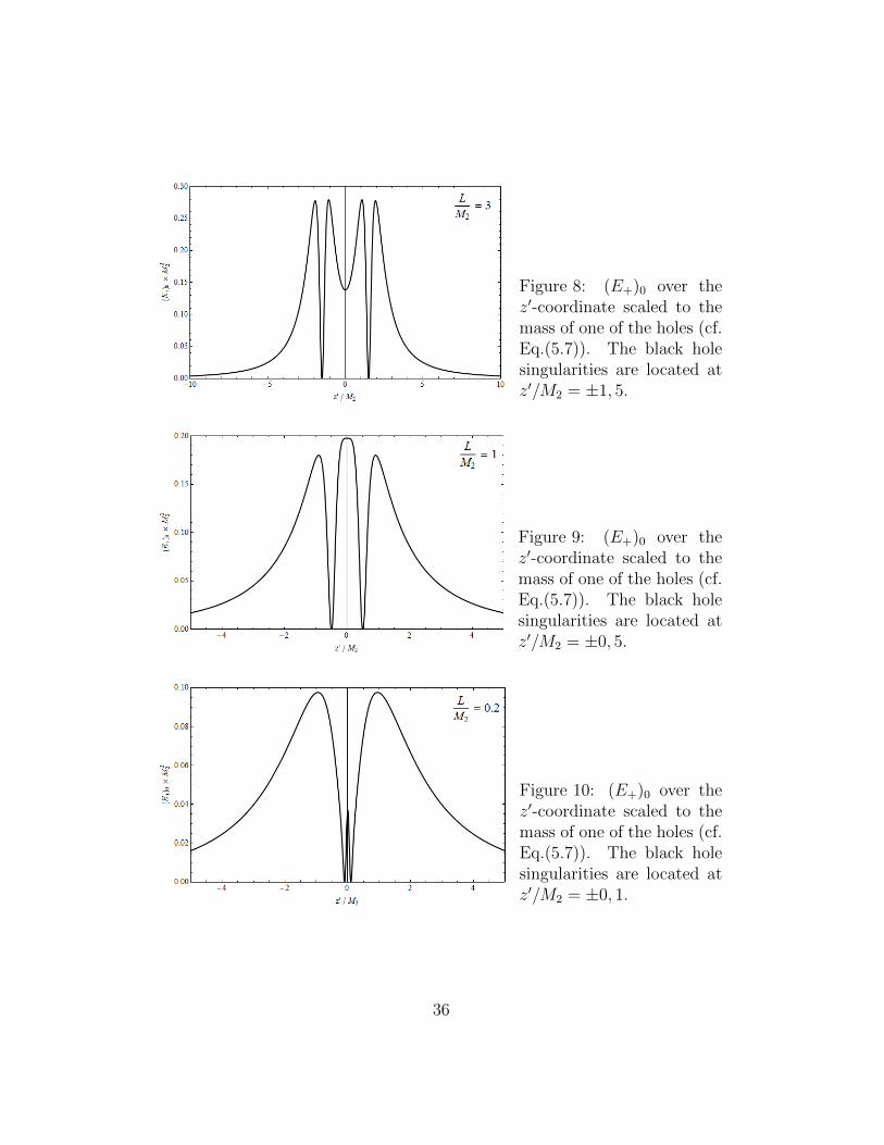
Figure 8: (E+)0 over thez′-coordinate scaled to themass of one of the holes (cf.Eq.(5.7)). The black holesingularities are located atz′/M2 = ±1, 5.

Figure 9: (E+)0 over thez′-coordinate scaled to themass of one of the holes (cf.Eq.(5.7)). The black holesingularities are located atz′/M2 = ±0, 5.

Figure 10: (E+)0 over thez′-coordinate scaled to themass of one of the holes (cf.Eq.(5.7)). The black holesingularities are located atz′/M2 = ±0, 1.

36

5.3.3 Infall Times

From the Weyl curvature Eq.(5.7) we can directly compute the infall timesto be:

τ2BH =πM2

8

√L+(L2−4x′2)2

(L++L−(L++1))6

[4L(x′L−L+ − 8x′3

)+ 4x′2

(L−L+ + 4x′2

)

+ L2(L−(L+ + 4

)+ 24x′2

)− 8x′L3 + L4

]−1/2

(5.9)

Figure 11: Infall times for a two black hole metric with equal masses. Thecollision time τc shows, when the two holes hit each other in the center ofthe coordinate system (red point). Observers outside of the red box fall intothe merged black hole, observers inside of the box fall into one of the holes,with the exception of z′ = 0. po and pi refer to the outer and inner minimalpeaks (blue points). The difference in their height is given by ∆p.

37

Considering that τ ∼ (E+)−1/20 (cf. Eq.(4.21)) the comparison of Figures

7 and 11 demonstrates that Weyl curvature and infall times are roughly“inverses” of each other. In the spacetime diagram 11 one point can besingled out, which is at z′ = 0. It refers to observers residing in the centerof the coordinate system that is due to the particular symmetry of the blackhole distribution not only the center of mass but also the point, where theattractions of each of the holes become equally strong. Theoretically thismeans that the observer at z′ = 0 is not drawn to any of the holes, but staysin the center.18 Eventually this allows us to compute the time of the twoholes’ collision by setting z′ = 0 in Eq.(5.9):

τc =πM2

8√

2

(L+ 2)5/2

L(5.10)

Unfortunately Eq.(5.9) cannot be solved for x′ analytically, but with Eq.(5.10)and specific choices of L we can find the corresponding spatial coordinatesnumerically. Thus for L = 10 we have z′m = ±9.06101, representing theminimal distance from which an observer must start to fall into the mergedblack hole.19 In Figure 11 the region, where observers fall into one of theseparated holes is coloured in red, though the point z′ = 0 must be excludedfrom that. A feature revealing the truly dynamic behaviour of the system isthe difference in height ∆p = 1− pi/p0 of the minimal peaks po and pi, withthe infall times for pi being slightly lower than for po. To the best of ourunderstanding this can only be explained by the simultaneous motion of theblack holes and the observers respectively. Though M1, p0 and pi executea congruent overall motion towards the other black hole M2, the motion ofp0 and pi relative to M1 is fairly different. While the outer observer movesin the same direction as the hole, the inner observer moves in the oppositedirection towards the hole, resulting in lower infall times. However, with∆p = 0.00004 this effect is not very prominent, so that to good approxima-tion the symmetry remains unbroken. Here we also want to point out thatfor observers falling from infinity the time it takes to fall into a double blackhole is to first-order approximation equal to the infall time of a single black

18Physically this configuration is not stable, since every infinitesimal perturbation wouldlead the observer to accelerate towards one of the holes.

19Other coordinate values might be found, if one considers observers falling from theother side of the Einstein-Rosen bridges.

38

hole containing the complete energy of the system:

τ2BH =π

2

z′3/2√2(M1 +M2)︸ ︷︷ ︸

cf. Eq.(2.42)

+O(z′

1/2)

(5.11)

This suggests that the energies lost to dynamical effects like gravitationalradiation must be rather small, which is in accordance with numerical simu-lations [21].

5.4 Double Black Hole Solutions with Unequal Masses

5.4.1 Infall Times

Generalizations to scenarios with different black hole masses are achievedeasily by introducing the inequality parameter

y ≡ M1

M2

, (5.12)

so that absolute values are parametrized in units of M2 with M1 → yM2. Thescaling of the mass M1 is then simply achieved by the scaling of y. However,this brings along some difficulty in understanding Figures 12 and 13. Whileit is intuitive that event horizons corresponding to the minimal peaks aredecreasing in size with xH = y/2, the decreasing of infall times around themuch smaller black hole M1 appears to contradict our findings of τ ∼ 1/

√M

(cf. Eq(2.42)). This puzzle can be solved immediately by remembering thatnot only the spatial coordinates but also the time coordinate in the vicinity ofM1 is given in the much larger units of M2. Eventually the small infall timesaround M1 are an illusion created by the parametrization with M2. One alsohas to keep in mind that the overall energy of the system MΣ = (y + 1)M2

decreases with y → 0, which makes it difficult to compare the various curvesin terms of absolute values. It naturally leads the maximum of the curves torise, while the infall times around M2 remain pretty stable, since it is affectedvery little by the change in interaction energy. This prominent feature isaccompanied by a shift of the maximum z′max towards the smaller black holeM1. As in the equal mass case we can straightforwardly conclude that thecollision times τc correspond to the maxima of the curves, so that observers

39

Figure 12: Infall times for a two black hole metric with unequal masses, i.e.M1 ≤M2. The maxima of the curves correspond to observers being attractedequally strong by each of the holes. The corresponding Weyl curvature (fory = 0.8) is given in appendix C.

to the left of the maximum fall into M1, while those to the right fall into M2.Unfortunately we can only solve the infall time equation

τ2BH =πM2

8

√L+(L2−4x′2)2

(L++L−(L++y))6

[4L(x′L−L+ − 8yx′3

)+ 4x′2

(L−L+ + 4yx′2

)

+ L2(L−(L+ + 4y

)+ 24yx′2

)− 8yx′L3 + yL4

]−1/2

(5.13)

for τc and its corresponding spatial coordinate z′c numerically. However, itremains unclear in how far the information about z′c is contained within theplot. Qualitatively we can only tell that 0 ≤ z′c < L/2, presumably near thecenter of mass, which is with Eq.(2.44), (2.45) and z± = ±L/2 at

z′com =m1z− +m2z+

m1 +m2

=L

2

y − 1

y + 1 + yL

M2. (5.14)

40

This equation is merely a Newtonian approximation and an exact analysiswould require full knowledge about gravitational wave radiation.

Figure 13: Infall times for a two black hole metric with unequal masses, i.e.M1 ≤M2. The maxima of the curves correspond to observers being attractedequally strong by each of the holes. The connected points represent thespacetime coordinates of the black holes’ collision estimated to be (τc, z

′com).

41

6 Conclusion

We have been successful in constructing metrics with multiple black holesand deriving analytically exact infall times into any of these holes in a fullydynamic scenario. To the best of the author’s knowledge this has not beenachieved before, thus making it superior to some of the purely numericalefforts of the past [22]. The formalism that we provide here covers manyof the known results from general relativity and can be applied to the colli-sion of black holes with arbitrary initial separations and mass configurations.Though our results implicate the truly dynamic behaviour of such systems,we remain unable to exactly quantify the effects of gravitational wave ra-diation. We believe that the information about these effects is containedwithin the equations we have, but so far we can only show that gravita-tional waves are negligible in first-order approximations. Consequently thequestion about the black hole’s mass, which forms from the merging of theseparated holes, remains unanswered and might be subject to future investi-gations. Also the discussion of section 5.3.2 about merging horizons requiresmore consideration than could be provided here. With the rough Newtonianapproximation of the collision coordinate z′com for the unequal mass case inmind (cf. Eq.(5.14)), it could be of interest to develop techniques that donot so heavily depend on the highly symmetrized situations that we considerhere.

Acknowledgement

I would like to express my gratitude to Prof. Dr. Kjell Rosquist, who ac-cepted me as a student and provided a comfortable working environmentwithin the Alba Nova facilities. His unreserved commitment and the manyopen-minded discussions ensured the success of this project. Moreover Ithank Stockholm University and all the people behind the ERASMUS ex-change programme for making this collaboration possible. Representative forthat I want to thank the study abroad coordinator Olaf Purkert. Addition-ally my thanks goes to Prof. Dr. Luciano Rezzolla, who provided supervisionof this work at the Goethe University in Frankfurt.

42

Appendix

A Notation Convention

Traditionally general relativity employs the Einstein summation convention:

AµBµ =

3∑µ=0

AµBµ = A0B

0 + A1B1 + A2B

2 + A3B3 (A.1)

As a subset of the Ricci calculus notation it allows to briefly relate ten-sor components to each other for tensors given in a coordinate basis. Thiscoordinate basis need not be specified explicitly and we will use the Latinalphabet to denote spacetime coordinate indices with the letters a − h ando − z running from 0 − 3, while spatial coordinate indices i − n run from1 − 3. When changing explicitly to an orthonormal frame (ONF), we willmake use of Greek letters so that spacetime coordinate indices run over thesecond half of the alphabet (µ, ν, ρ, ... = 0 − 3) and spatial coordinate in-dices run over the first half of the alphabet (α, β, γ, ... = 1− 3). Sometimeswe will emphasize the dimension of an object with a number in brackets,e.g. (3)Tab for a three-dimensional tensor. Throughout this work we willadopt the metric signature (−,+,+,+) for four-dimensional spacetime and(+,+,+) for three-dimensional space. Much of section 3.1 follows the bookof Baumgarte and Shapiro [30], where abstract index notation is used. Thisnotation merely relates tensors but not their components to each other, sinceit abstains from choosing any coordinate frame. However, the distinction be-tween the Einstein summation convention and the abstract index notationis of minor importance for the development of the formalism so that we willmake it visible only where necessary. Also we set G = 1 = c.

43

B ADM equations

in orthonormal frame variables

Here we list the evolution and constraint equations in terms of orthonormalframe variables introduced in section 3.4. They are taken from [25] and holdtrue for vacuum solutions, vanishing cosmological constant and na = 0. Moregeneral expressions and an extensive discussion can be found in [41].

Evolution Equations

e0(Θ) = −1

3Θ2 − 2σ2 + 2ω2 (B.1)

e0(σαβ) = −Θσαβ + 2ω(αΩβ) − Sαβ −2

3δαβωγΩ

γ + 2εγδ(αΩγσβ)δ (B.2)

e0(ωα) = −2

3Θωα + σαβ ω

β − εαβγωβΩγ (B.3)

e0(Eαβ) = −ΘEαβ + 3σ(αγE

β)γ + εγδ(α[(eγ − aγ)Hβ)

δ − (ωγ − 2Ωγ)Eβ)δ

]− δαβ

[σγδE

γδ − nγδHγδ]

+1

2nγγH

αβ − 3n(αγH

β)γ (B.4)

e0(Hαβ) = −ΘHαβ + 3σ(αγH

β)γ + εγδ(α[(eγ − aγ)Eβ)

δ − (ωγ − 2Ωγ)Hβ)δ

]− δαβ

[σγδH

γδ − nγδEγδ]

+1

2nγγE

αβ − 3n(αγE

β)γ (B.5)

e0(aα) = −1

3(δαβeβ + aα)Θ +

1

2(eβ − 2aβ)σαβ

− 1

2εαβγ(eβ − 2aβ)(ωγ − Ωγ) (B.6)

e0(nαβ) = −1

3Θnαβ − δγ(αeγ(ω

β) − Ωβ)) + 2σ(αγ n

β)γ

+ δαβeγ(ωγ − Ωγ)− εγδ(α

[eγσ

β)δ − 2nβ)

γ(ωδ − Ωδ)]

(B.7)

44

Constraint Equations

0 = −1

3Θ2 + σ2 − ω2 − 2ωαΩα − 1

2(3)R (B.8)

Eαβ =1

3Θσαβ − σαγσγβ − ωαωβ − 2ω(αΩβ)

+1

3δαβ[2σ2 + ω2 + 2ωγΩ

γ] + Sαβ (B.9)

Hαβ =1

2nγγ σαβ − 3nγ(ασβ)γ −

1

3δαβ

[(eγ + aγ)ω

γ − 3nγδσγδ]

+ εγδ(α

[(e|γ| − a|γ|) σβ)γ − nβ)γωδ

]+ (e(α + a(α) ωβ) (B.10)

0 = −2

3δαβeβΘ + (eβ − 3aβ) σαβ + nαβ ω

β

− εαβγ[(eβ − aβ) ωγ + nβδσ

δγ

](B.11)

0 = (eβ − 2aβ) nαβ − 2

3Θωα − 2σαβ ω

β + εαβγ[eβaγ + 2ωβΩγ

](B.12)

0 = (eβ − 2aα) ωα (B.13)

0 = (eβ − 3aβ) Eαβ + 3ωβHαβ − εαβγ

[σβδH

δγ + nβδE

δγ

](B.14)

0 = (eβ − 3aβ) Hαβ − 3ωβEαβ + εαβγ

[σβδE

δγ − nβδHδ

γ

](B.15)

Other Relations

(3)R = 2(eα − 3aα) aα − 1

2bαα (B.16)

Sαβ = e(αaβ) + bαβ −1

3δαβ[eγa

γ + bγγ]− εγδ(α(e|γ| − 2a|γ|)nβ)δ (B.17)

bαβ = 2nαγnγβ − nγγnαβ (B.18)

Ωα =1

2εαβγeβ

aeγa (B.19)

eµ = eµa∂a (B.20)

The 1-index object aα and the 2-index object nαβ are defined by the com-mutation relation

[eβ, eγ] = (2a[βδαγ] + εβγδn

δα) eα. (B.21)

45

C Weyl Curvature for Unequal Masses

Figure 14: Weyl curvature for a two black hole metric with unequal masses,i.e. M1 ≤ M2. The corresponding infall times (for y = 0.4) are given inFigure 12.

(E+)0 =24L+

(L2 − 4x′2

)2

M22

(L+ + L−

(L+ + y

))6

×[4L(x′L−L+ − 8yx′3

)+ 4x′2

(L−L+ + 4yx′2

)+ L2

(L−(L+ + 4y

)+ 24yx′2

)− 8yx′L3 + yL4

](C.1)

46

References

[1] John Michell, in a letter to Henry Cavendish, archived in Phil. Trans.R. Soc. Lond. (1784) 74

[2] Charles Coulston Gillispie, Pierre-Simon Laplace, 1749-1827: a life inexact science, Princeton University Press (1997)

[3] Karl Schwarzschild, Uber das Gravitationsfeld eines Massenpunktes nachder Einsteinschen Theorie, Deutsche Akademie der Wissenschaften zuBerlin (1916)

[4] Hans Reissner, Uber die Eigengravitation des elektrischen Feldes nachder Einsteinschen Theorie, Annalen der Physik 50: 106120 (1916)

[5] Gunnar Nordstrom, On the Energy of the Gravitational Field in Ein-stein’s Theory, Verhandl. Koninkl. Ned. Akad. Wetenschap., Afdel.Natuurk., Amsterdam 26: 12011208 (1918)

[6] J.R. Oppenheimer and G.M. Volkoff, On Massive Neutron Cores, Phys-ical Review 55 (4): 374381 (1939)

[7] Jocelyn Bell Burnell and Antony Hewish, Observation of a Rapidly Pul-sating Radio Source, Nature 217 (5130): 709713 (1968)

[8] Roy Kerr, Gravitational Field of a Spinning Mass as an Example ofAlgebraically Special Metrics, Physical Review Letters 11 (5): 237238(1963)

[9] Ezra Newman and Allen Janis, Note on the Kerr Spinning-Particle Met-ric, Journal of Mathematical Physics 6 (6): 915917 (1965)

[10] Ezra Newman et al., Metric of a Rotating, Charged Mass, Journal ofMathematical Physics 6 (6): 918919 (1965)

[11] Charles Thomas Bolton, Identification of Cygnus X-1 with HDE 226868,Nature 235 (5336): 271273 (1972)

[12] James M. Bardenn, Brandon Carter, Stephen W. Hawking, The FourLaws of Black Hole Mechanics, Commun. math. Phys. 31, 161-170 (t973)

[13] Stephen W. Hawking, Particle Creation by Black Holes, Commun. math.Phys. 43, 199220 (1975)

47

[14] Leonard Susskind, The World as a Hologram, Journal of MathematicalPhysics 36 (11): 63776396 (1995)

[15] Juan Maldacena, The Large N limit of superconformal field theoriesand supergravity, Advances in Theoretical and Mathematical Physics2: 231252 (1998)

[16] R. Antonucci, Unified Models for Active Galactic Nuclei and Quasars,Annual Reviews in Astronomy and Astrophysics 31 (1): 473521 (1993)

[17] R. Schodel, A star in a 15.2-year orbit around the supermassive blackhole at the centre of the Milky Way, Nature 419 (6908): 694696 (2002)

[18] S. Dimopoulos and G. L. Landsberg, Black Holes at the Large HadronCollider, Phys. Rev. Lett. 87 (16): 161602 (2001)

[19] S. B. Giddings and S. D. Thomas, High-energy colliders as black hole fac-tories: The End of short distance physics, Phys. Rev. D 65 (5): 056010(2002)

[20] J. M. Weisberg, J. H. Taylor and L. A. Fowler, Gravitational waves froman orbiting pulsar, Scientific American 245: 7482 (1981)

[21] Peter Anninos et al., Collision of Two Black Holes, Physical Review:Volume 71, Number 18 (1993)

[22] Peter Anninos et al., Head-on collision of two equal mass black holes,Phys. Rev. D: Volume 52, Number 8 (1995)

[23] Peter Anninos et al., Head-on collision of two black holes: Comparisonof different approaches, Phys. Rev. D: Volume

[24] Peter Anninos, Steven Brandt, Head-On Collision of Two Unequal MassBlack Holes, Physical Review: Volume 81, Number 3 (1998)

[25] Timothy Clifton, Daniele Gregoris, Kjell Rosquist and Reza Tavakola,Exact evolution of discrete relativistic cosmological models, Journal ofCosmology and Astroparticle Physics (2013)

[26] S.W. Hawking, Black Holes in General Relativity, (Cambridge U.), Oct1971; Published in Commun.Math.Phys. 25 (1972) 152-166

[27] Sean M. Carroll, Spacetime and Geometry, Pearson Education, Inc.,published as Addison Wesley, San Francisco (2004)

48

[28] Albert Einstein, Die Feldgleichungen der Gravitation, Sitzungsberichteder Preussischen Akademie der Wissenschaften zu Berlin: 844-847(1915)

[29] Lewis Ryder, Introduction to General Relativity, Cambridge UniversityPress (2009)

[30] Thomas W. Baumgarte and Stuart L. Shapiro, Numerical Relativity,Cambridge University Press (2010)

[31] A.K. Raychaudhuri, S. Banerji, A. Banerjee, General Relativity, Astro-physics and Cosmology, Springer Verlag, University of Michigan (1992)

[32] C.W. Misner, K.S. Thorne, J.A. Wheeler, Gravitation, Copyright byW.H. Freeman and Company, USA (1973)

[33] Dieter R. Brill, Richard W. Lindquist, Interaction Energy in Geometro-statics, Physical Review: Volume 131, Number 1 (1963)

[34] Stephen W. Hawking, Gravitational Radiation from Colliding BlackHoles, Physical Review: Volume 26, Number 21 (1971)

[35] Stephen W. Hawking, Black Holes in General Relativity, Commun.math. Phys. 25, 152166 (1972)

[36] Stephen W. Hawking, Black holes and thermodynamics, Physical ReviewD: Volume 13, Number 2 (1976)

[37] Helena Engstrom, Properties of mass distributions for discrete cosmol-ogy, Stockholm University (2013)

[38] Jurgen Ehlers, Beitrage zur relativistischen Mechanik kontinuierlicherMedien, Akad. Wiss. Lit. Mainz, Abhandl. Math.-Nat. Kl. 11 (1961)

[39] Andrej Cadez, Apparent Horizons in the Two-Black-Hole Problem, An-nals of Physics 83, 449-457 (1974)

[40] Henk van Elst, George F. R. Ellis, The covariant approach to LRS perfectfluid spacetime geometries, Class. Quantum Grav. 13 (1996) 10991127

[41] Henk van Elst, Claes Uggla, General Relativistic 1+3 OrthonormalFrame Approach Revisited, Class. Quantum Grav. 14 2673 (1997)

[42] Sotirios Bonanos, Riemannian Geometry & Tensor Calculus @ Mathe-matica, http://www.inp.demokritos.gr/~sbonano/RGTC/

49