J. Math. Fluid Mech.c© 2014 Springer BaselDOI 10.1007/s00021-014-0168-3

Journal of MathematicalFluid Mechanics

An Exact Solution for Nonlinear Internal Equatorial Wavesin the f -Plane Approximation

Hung-Chu Hsu

Communicated by A. Constantin

Abstract. We present an exact solution of the nonlinear governing equations for internal geophysical water waves propagatingwestward in the f -plane approximation near the equator. We show that the mass transport velocity induced by this internalequatorial wave is eastward.

Mathematics Subject Classification (2010). Primary 76B55, 86A05, 76E30.

Keywords. Nonlinear internal wave, geophysical waves, exact solution.

1. Introduction

Oceanic variability in the equatorial oceans has been studied extensively over the past several decades,especially the interplay between the flows and the currents in the ocean and atmosphere, which are keyfactors in explaining the El Nino phenomenon. An interesting feature is that the thermocline, whichseparates warm surface water from colder deep water, is basically propagating as an oscillation of aninterface. The field data examined in Moum et al. [1] shows the importance of large amplitude internalwaves in the dynamics of the upper-equatorial oceans. Smyth et al. [2] used linear equatorial wave theoryto discuss the equatorially trapped waves. However, Fedorov and Melville [3] and Greatbatch [4] provideevidence that nonlinear equatorial processes are important in modeling the equatorial waves. This remainsrelatively poorly understood from a theoretical point of view.

Recently, some exact solutions describing nonlinear equatorial flows in the Lagrangian framework wereobtained. The solution in Lagrangian coordinates was found for periodic in a homogenous fluid by Gerstner[5], and rediscovered by Rankine [6]. Constantin [7,8] and Henry [9] offer a modern treatment of Gerstnerswave. This flow has been used to describe a number of interesting studies within the class of gravity edgewaves (cf. Ehrnstrom et al. [10], Henry and Mustafa [11], Johnson [12], Constantin [13], Stuhlmeier [14],Matioc [15], Hsu [16]). In Constantin [17] equatorially trapped wind waves were presented—see alsoConstantin and Germain [18], and Hsu [19]. In Constantin [20] internal waves describing the oscillationof the thermocline as a density interface separating two layers of constant density, with the lower layermotionless, were presented in the β-plane approximation. Hsu [21] extend the flow in Constantin [20] tostudy the geophysical internal waves underlying a uniform current. Constantin [22] demonstrated thatthe f -plane approximation is physically realistic for certain equatorial flows.

The aim of the present paper is to provide an explicit nonlinear solution for internal geophysical wavespropagating westward in the layer above the thermocline and beneath the near-surface layer in whichwind effect are important, valid in the f -plane approximation. The solution is presented in Lagrangiancoordinates by describing the circular path of each particle. The internal equatorially wave is valid withina narrow equatorial band that is symmetric about the equator. In contrast to the situation in the β-planeapproximation, investigated in Constantin [18,23], we construct westward propagating waves.

This work was completed with the support of our TEX-pert.

H.-C. Hsu JMFM

2. Preliminaries

The Earth is taken to be a sphere of radius (R = 6,371 km), rotating with constant rotational speedΩ = 7.29 × 10−5 rad s−1 round the polar axis toward the east, in a rotating frame with the origin at apoint on the Earths surface, so that the Cartesian coordinates (x, y, z) represent longitude, latitude, andthe local vertical, respectively. The governing equations for geophysical ocean waves are, cf. Pedlosky[24], the Euler’s equation

⎧⎪⎨

⎪⎩

ut + uux + vuy + wuz + 2Ωw cos φ − 2Ωv sin φ = − 1ρPx,

vt + uvx + vvy + wvz + 2Ωu sin φ = − 1ρPy,

wt + uwx + vwy + wwz − 2Ωu cos φ = − 1ρPz − g,

(2.1)

coupled with the equation of mass conservation

ρt + uρx + vρy + wρz = 0 (2.2)

and with the incompressibility constraint

ux + vy + wz = 0. (2.3)

Here t stands for time, φ for latitude, g = 9.81 ms−2 is the (constant) gravitational acceleration at theEarths surface, and ρ is the waters density, while P is the pressure. Since we restrict our attention toa symmetric band of width of about 250 km on each side of the equator, we neglect the variations ofthe Coriolis parameter and use the f -plane approximation. For the reasonableness of this approxima-tion within this physical setting we refer to the discussion in Constantin [19]. Note that the f -planeapproximation amounts to replacing the Euler equation (2.1) by

⎧⎪⎨

⎪⎩

ut + uux + vuy + wuz + 2Ωw = − 1ρPx,

vt + uvx + vvy + wvz = − 1ρPy,

wt + uwx + vwy + wwz − 2Ωu = − 1ρPz − g,

(2.4)

We work with a two-layer model: two layers of constant densities, separated by a sharp interface thethermocline. Let z = η(x, y, t) be the equation of the thermocline. The oscillations of this interfacepropagate in the longitudinal direction at constant speed c. The upper boundary of the region M(t) ontop of the thermocline and below the near-surface layer L(t) , where wind effects are not negligible, isgiven by z = η+(x − ct). Beneath the thermocline the water has a constant density ρ+ and is still: atevery instant t we have u = v = w = 0 for z < η(x − ct). From (2.4) we get

P = P0 − ρ+gz for z < η(x, y, t), (2.5)

for some constant P0. We study the westward propagation of internal geophysical waves with vanishingmeridional velocity (v = 0) in the region M(t), without addresing the interaction of geophysical wavesand wind waves in the region L(t). Throughout M(t) the water has constant density ρ0 < ρ+ , the typicalvalue of the reduced gravity

g = gρ+ − ρ0

ρ0(2.6)

being 6× 10−3 ms−2, cf. Fedorov and Brown [25]. We want travelling waves solutions (u(x− ct, z), w(x−ct, z), η(x − ct) and η+(x − ct)) of the Eulers equations in the form

⎧⎪⎨

⎪⎩

ut + uux + wuz + 2Ωw = − 1ρPx,

Py = 0,

wt + uwx + wwz − 2Ωu = − 1ρPz − g,

(2.7)

An Exact Solution for Nonlinear Internal Equatorial Waves

in η(x − ct) < z < η+(x − ct) , coupled with the incompressibility condition

ux + wz = 0 in η(x − ct) < z < η+(x − ct). (2.8)

and with the boundary condition

P = P0 − ρ+gz on z = η(x − ct). (2.9)

3. Main Result

In this section, we will present the exact solution, representing waves travelling westwards in the longi-tudinal direction, at a constant speed of propagation. Throughout this paper, the Lagrangian positions(x, y, z) of the fluid particles are given as functions of labeling variables (q, r, s) and time t by

⎧⎪⎨

⎪⎩

x = q − 1ke−kr sin[k(q − ct)],

y = s,

z = r − 1ke−kr cos[k(q − ct)],

(3.1)

where k is the wave number. The parameter q runs over the whole real line, while s ∈ [−s0, s0] , wheres0 ≈ 250 km, cf. the discussion in Constantin [18], is the equatorial radius of deformation. As for thelabel r, we require r ∈ [r0, r+] , with the two positive numbers to be specified by later on. The particlessubject to (3.1) describe circles. This is like the flow discovered by Gerstner [5]; see the comments inConstantin [7,8] and Henrys [9]. This situation is unlike that in the irrotational flow beneath a Stokeswave, cf. the discussion in Constantin [26], Henry [27], Constantin and Strauss [28]. This suggests shearedflow, an aspect that we address in Section 4 by describing the vorticity of the flow (3.1). The equation(3.1) represent the flow beneath a Gerstner wave propagating westward at constant speed

c =Ω −

√Ω2 + kg

k<0, (3.2)

so that (3.1) defines internal equatorial waves propagating westward. Note that for the case of

c =Ω +

√Ω2 + kg

k> 0,

the internal equatorial waves propagating eastward also exists, which had been discussed by Constantin[18] in the β-plane approximation. To verify that (3.1) is a solution, we first observe that the determinantof the matrix ⎛

⎜⎜⎝

∂x∂q

∂y∂q

∂z∂q

∂x∂s

∂y∂s

∂z∂s

∂x∂r

∂y∂r

∂z∂r

⎞

⎟⎟⎠ =

⎛

⎜⎝

1 − e−ξ cos θ 0 e−ξ sin θ

0 1 0

e−ξ sin θ 0 1 + e−ξ cos θ

⎞

⎟⎠ (3.3)

equals 1 − e−2ξ, whereξ = kr, θ = k(q − ct) (3.4)

Due to the time-independence of the determinant, the fluid flow is volume-preserving, so that (2.3) holds.We require that the labeling variables satisfy

r ≥ r∗ (3.5)

for some r∗ > 0. We rewrite the Eulers equation (2.4) as⎧⎪⎪⎨

⎪⎪⎩

DuDt + 2Ωw = − 1

ρPx,

DvDt = − 1

ρPy,

DwDt − 2Ωu = − 1

ρPz − g.

(3.6)

H.-C. Hsu JMFM

From (3.1) we compute the velocity and acceleration of a particle as⎧⎪⎪⎨

⎪⎪⎩

u = DxDt = ce−ξ cos θ,

v = DyDt = 0,

w = DzDt = −ce−ξ sin θ,

(3.7)

respectively, ⎧⎪⎪⎨

⎪⎪⎩

DuDt = kc2e−ξ sin θ,

DvDt = 0,

DwDt = kc2e−ξ cos θ.

(3.8)

Since⎛

⎜⎝

Pq

Ps

Pr

⎞

⎟⎠ =

⎛

⎜⎜⎝

∂x∂q

∂y∂q

∂z∂q

∂x∂s

∂y∂s

∂z∂s

∂x∂r

∂y∂r

∂z∂r

⎞

⎟⎟⎠

⎛

⎜⎝

Px

Py

Pz

⎞

⎟⎠ , (3.9)

and, in view of (3.7)–(3.8), (3.6) can be written as

Px = −ρ0(kc2 − 2Ωc)e−ξ sin θ, (3.10)Py = 0, (3.11)

Pz = −ρ0[kc2e−ξ cos θ − 2Ωce−ξ cos θ + g], (3.12)

we have that (3.9) is the same as

Pq = −ρ0[kc2 − 2Ωc + g]e−ξ sin θ, (3.13)Ps = 0, (3.14)

Pr = −ρ0[kc2 − 2Ωc + g]e−ξ cos θ − ρ0(kc2 − 2Ωc)e−2ξ − ρ0g, (3.15)

Now, the gradient of the expression

P = ρ0[kc2 − 2Ωc + g]

ke−ξ cos θ + ρ0

(kc2 − 2Ωc)2k

e−2ξ − ρ0gr + P0. (3.16)

with respect to the labeling variables is precisely the right-hand side of (3.13)–(3.15). The choice r = r0

corresponds to the thermocline z = η(x − ct), (3.16) at the thermocline is the same as (2.9) if thedispersion equation

ρ0(kc2 − 2Ωc + g) = ρ+g (3.17)holds. We require c < 0 for our westward-propagating waves. Thus

c =Ω −

√Ω2 + kg

k. (3.18)

This shows that (3.1)–(3.2) yield a solution to (2.4)–(2.9), the thermocline being determined by settingr = r0 , where r0 is the unique solution of the equation

P ∗0 = r +

12k

exp (−2kr) , (3.19)

with

P ∗0 =

P0 − P0

ρ0g.

The functionr �→ r +

12k

exp (−2kr)

is a strictly increasing bijection, so that if

P ∗0 >

12k

, (3.20)

An Exact Solution for Nonlinear Internal Equatorial Waves

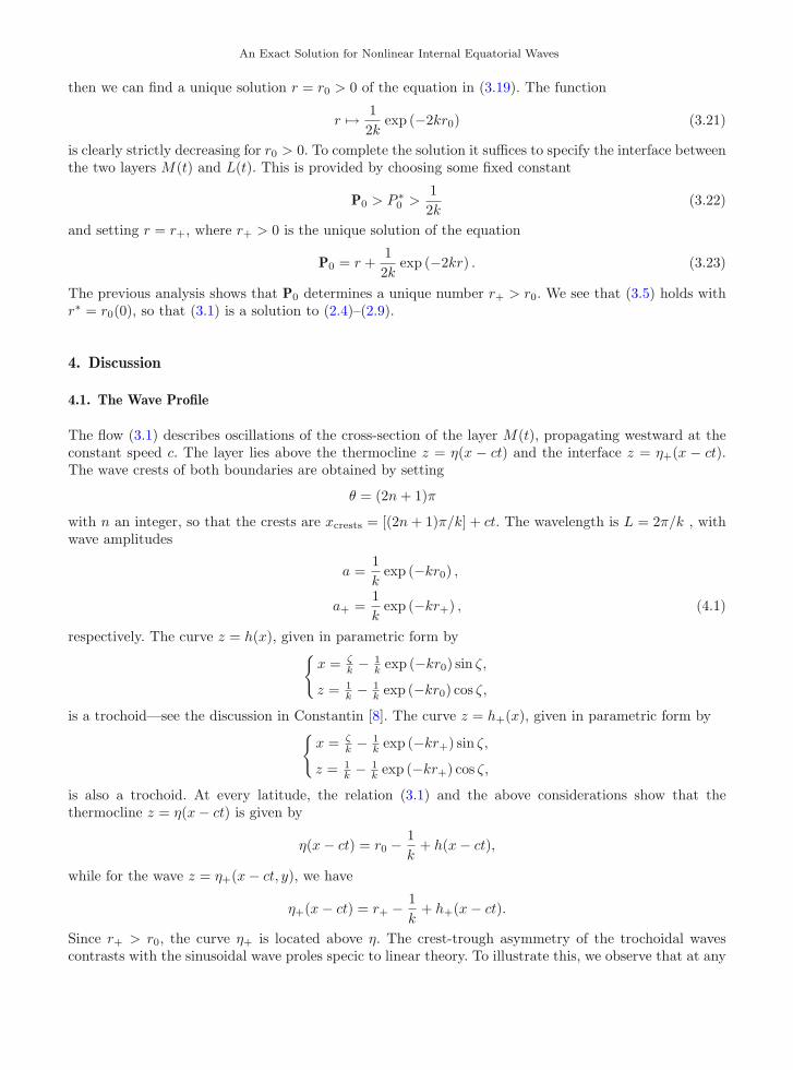
then we can find a unique solution r = r0 > 0 of the equation in (3.19). The function

r �→ 12k

exp (−2kr0) (3.21)

is clearly strictly decreasing for r0 > 0. To complete the solution it suffices to specify the interface betweenthe two layers M(t) and L(t). This is provided by choosing some fixed constant

P0 > P ∗0 >

12k

(3.22)

and setting r = r+, where r+ > 0 is the unique solution of the equation

P0 = r +12k

exp (−2kr) . (3.23)

The previous analysis shows that P0 determines a unique number r+ > r0. We see that (3.5) holds withr∗ = r0(0), so that (3.1) is a solution to (2.4)–(2.9).

4. Discussion

4.1. The Wave Profile

The flow (3.1) describes oscillations of the cross-section of the layer M(t), propagating westward at theconstant speed c. The layer lies above the thermocline z = η(x − ct) and the interface z = η+(x − ct).The wave crests of both boundaries are obtained by setting

θ = (2n + 1)π

with n an integer, so that the crests are xcrests = [(2n + 1)π/k] + ct. The wavelength is L = 2π/k , withwave amplitudes

a =1k

exp (−kr0) ,

a+ =1k

exp (−kr+) , (4.1)

respectively. The curve z = h(x), given in parametric form by{

x = ζk − 1

k exp (−kr0) sin ζ,

z = 1k − 1

k exp (−kr0) cos ζ,

is a trochoid—see the discussion in Constantin [8]. The curve z = h+(x), given in parametric form by{

x = ζk − 1

k exp (−kr+) sin ζ,

z = 1k − 1

k exp (−kr+) cos ζ,

is also a trochoid. At every latitude, the relation (3.1) and the above considerations show that thethermocline z = η(x − ct) is given by

η(x − ct) = r0 − 1k

+ h(x − ct),

while for the wave z = η+(x − ct, y), we have

η+(x − ct) = r+ − 1k

+ h+(x − ct).

Since r+ > r0, the curve η+ is located above η. The crest-trough asymmetry of the trochoidal wavescontrasts with the sinusoidal wave proles specic to linear theory. To illustrate this, we observe that at any

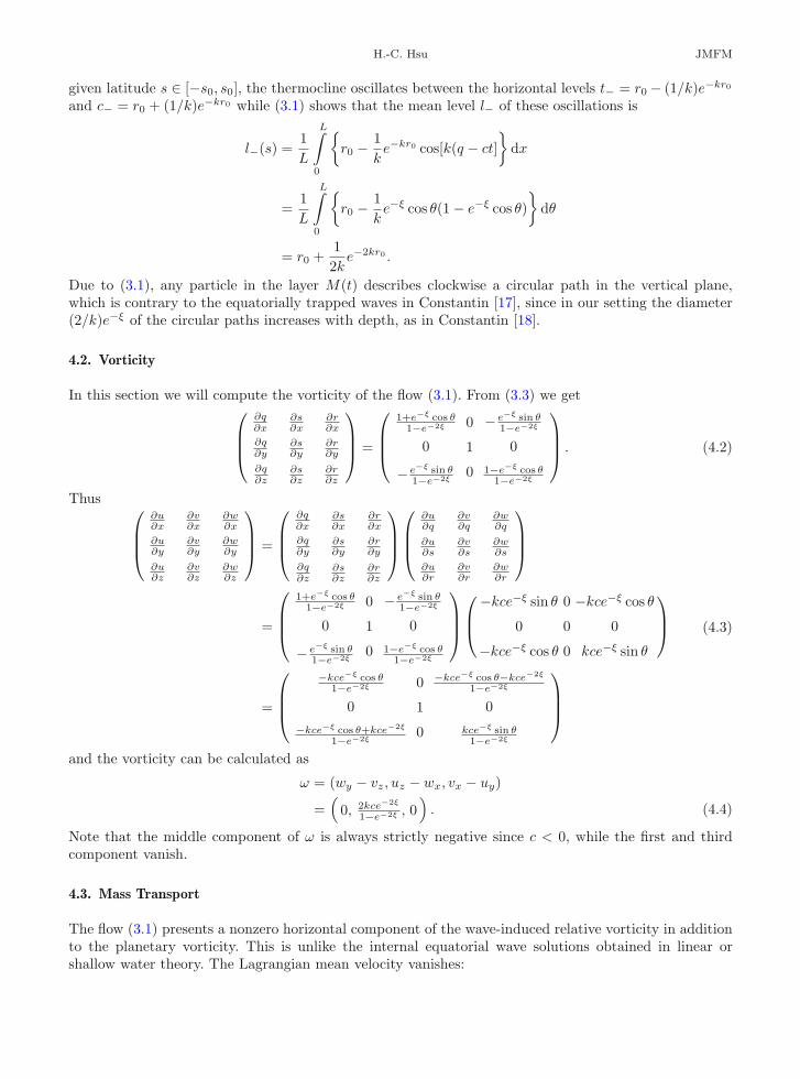
H.-C. Hsu JMFM

given latitude s ∈ [−s0, s0], the thermocline oscillates between the horizontal levels t− = r0 − (1/k)e−kr0

and c− = r0 + (1/k)e−kr0 while (3.1) shows that the mean level l− of these oscillations is

l−(s) =1L

L∫

0

{

r0 − 1k

e−kr0 cos[k(q − ct]}

dx

=1L

L∫

0

{

r0 − 1k

e−ξ cos θ(1 − e−ξ cos θ)}

dθ

= r0 +12k

e−2kr0 .

Due to (3.1), any particle in the layer M(t) describes clockwise a circular path in the vertical plane,which is contrary to the equatorially trapped waves in Constantin [17], since in our setting the diameter(2/k)e−ξ of the circular paths increases with depth, as in Constantin [18].

4.2. Vorticity

In this section we will compute the vorticity of the flow (3.1). From (3.3) we get⎛

⎜⎜⎝

∂q∂x

∂s∂x

∂r∂x

∂q∂y

∂s∂y

∂r∂y

∂q∂z

∂s∂z

∂r∂z

⎞

⎟⎟⎠ =

⎛

⎜⎜⎝

1+e−ξ cos θ1−e−2ξ

0

− e−ξ sin θ1−e−2ξ

0

1

0

− e−ξ sin θ1−e−2ξ

01−e−ξ cos θ

1−e−2ξ

⎞

⎟⎟⎠ . (4.2)

Thus⎛

⎜⎜⎝

∂u∂x

∂v∂x

∂w∂x

∂u∂y

∂v∂y

∂w∂y

∂u∂z

∂v∂z

∂w∂z

⎞

⎟⎟⎠ =

⎛

⎜⎜⎝

∂q∂x

∂s∂x

∂r∂x

∂q∂y

∂s∂y

∂r∂y

∂q∂z

∂s∂z

∂r∂z

⎞

⎟⎟⎠

⎛

⎜⎜⎝

∂u∂q

∂v∂q

∂w∂q

∂u∂s

∂v∂s

∂w∂s

∂u∂r

∂v∂r

∂w∂r

⎞

⎟⎟⎠

=

⎛

⎜⎜⎝

1+e−ξ cos θ1−e−2ξ

0

− e−ξ sin θ1−e−2ξ

0

1

0

− e−ξ sin θ1−e−2ξ

01−e−ξ cos θ

1−e−2ξ

⎞

⎟⎟⎠

⎛

⎜⎝

−kce−ξ sin θ 0 −kce−ξ cos θ

0 0 0

−kce−ξ cos θ 0 kce−ξ sin θ

⎞

⎟⎠

=

⎛

⎜⎜⎝

−kce−ξ cos θ1−e−2ξ

0−kce−ξ cos θ+kce−2ξ

1−e−2ξ

0

1

0

−kce−ξ cos θ−kce−2ξ

1−e−2ξ

0kce−ξ sin θ

1−e−2ξ

⎞

⎟⎟⎠

(4.3)

and the vorticity can be calculated as

ω = (wy − vz, uz − wx, vx − uy)

=(

0, 2kce−2ξ

1−e−2ξ , 0)

. (4.4)

Note that the middle component of ω is always strictly negative since c < 0, while the first and thirdcomponent vanish.

4.3. Mass Transport

The flow (3.1) presents a nonzero horizontal component of the wave-induced relative vorticity in additionto the planetary vorticity. This is unlike the internal equatorial wave solutions obtained in linear orshallow water theory. The Lagrangian mean velocity vanishes:

An Exact Solution for Nonlinear Internal Equatorial Waves

〈u〉L =1T

T∫

0

u(q − ct, r)dt = 0. (4.5)

since the average of u, given by (3.7), over a wave period T = L/c , vanishes. A fixed depth z0 ∈ [c−, t+]is obtained as

z0 = r − 1k

e−ξ cos θ. (4.6)

From (4.6) we getr = α(q − ct, z0). (4.7)

Differentiating (4.7) with respect to the q variable yields

0 = αq + αqe−ξ cos θ + e−ξ sin θ, (4.8)

so that

αq = − e−ξ sin θ

1 + e−ξ cos θ. (4.9)

Thus the Eulerian mean velocity 〈u〉E(z0) at the fixed depth z0 is

c + 〈u〉E(z0) =c

L

L/c∫

0

[c + u(x − ct, z0)]dt

=1L

L∫

0

[c + u(x − ct, z0)]dt

=1L

L∫

0

{c + u(q − ct, α(q − ct, z0))}∂x

∂qdq

=1L

L∫

0

{c + u(q − ct, α(q − ct, z0))} × (1 + e−ξαq sin θ − e−ξ cos θ

)dq

=1L

L∫

0

c(1 + e−ξ cos θ) ×(

1 − e−ξ cos θ − e−2ξsin2θ

1 + e−ξ cos θ

)

dq

=1L

L∫

0

c(1 − e−2ξ)dq.

Thus

〈u〉E(z0) = − c

L

L∫

0

e−2kα(q,z0)dq ∈ (−c, 0), (4.10)

which shows that the Eulerian mean flow is eastward. The Stokes drift, defined by Longuet-Higgins [29]as the difference between the Lagrangian and the Eulerian mean velocities, is consequently westward (theLagrangian mean flow being zero). Differentiating (4.6) with respect to z0, we obtain

1 = αz0 + αz0e−ξ cos θ,

so that

αz0 =1

1 + e−ξ cos θ> 0.

H.-C. Hsu JMFM

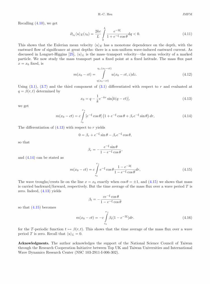
Recalling (4.10), we get

∂z0〈u〉E(z0) =2kc

L

L∫

0

e−2ξ

1 + e−ξ cos θdq < 0. (4.11)

This shows that the Eulerian mean velocity 〈u〉E has a monotone dependence on the depth, with theeastward flow of significance at great depths: there is a non-uniform wave-induced eastward current. Asdiscussed in Longuet-Higgins [25], 〈u〉L is the mass–transport velocity—the mean velocity of a markedparticle. We now study the mass transport past a fixed point at a fixed latitude. The mass flux pastx = x0 fixed, is

m(x0 − ct) =

η+(x0−ct)∫

η(x0−ct)

u(x0 − ct, z)dz. (4.12)

Using (3.1), (3.7) and the third component of (3.1) differentiated with respect to r and evaluated atq = β(r, t) determined by

x0 = q − 1k

e−kr sin[k(q − ct)], (4.13)

we get

m(x0 − ct) = c

r+∫

r0

[e−ξ cos θ](1 + e−ξ cos θ + βre

−ξ sin θ)dr, (4.14)

The differentiation of (4.13) with respect to r yields

0 = βr + e−ξ sin θ − βre−ξ cos θ,

so that

βr = − e−ξ sin θ

1 − e−ξ cos θ,

and (4.14) can be stated as

m(x0 − ct) = c

r+∫

r0

e−ξ cos θ1 − e−2ξ

1 − e−ξ cos θdr, (4.15)

The wave troughs/crests lie on the line x = x0 exactly when cos θ = ±1, and (4.15) we shows that massis carried backward/forward, respectively. But the time average of the mass flux over a wave period T iszero. Indeed, (4.13) yields

βt = − ce−ξ cos θ

1 − e−ξ cos θ

so that (4.15) becomes

m(x0 − ct) = −c

r+∫

r0

βt(1 − e−2ξ)dr. (4.16)

for the T -periodic function t �→ β(r, t). This shows that the time average of the mass flux over a waveperiod T is zero. Recall that 〈u〉L = 0.

Acknowledgments. The author acknowledges the support of the National Science Council of Taiwanthrough the Research Cooperation Initiative between Top UK and Taiwan Universities and InternationalWave Dynamics Research Center (NSC 103-2911-I-006-302).

An Exact Solution for Nonlinear Internal Equatorial Waves

References

[1] Moum, J.N., Nash, J.D., Smyth, W.D.: Narrowband oscillations in the upper equatorial ocean. Part I: interpretationas shear instability. J. Phys. Oceanogr. 41, 397–411 (2011)

[2] Smyth, W.D., Moum, J.N., Nash, J.D.: Narrowband oscillations in the upper equatorial ocean. Part II: properties ofshear instabilities. J. Phys. Oceanogr. 41, 412–428 (2011)

[3] Fedorov, A.V., Melville, W.K.: Kelvin fronts on the equatorial thermocline. J. Phys. Oceanogr. 30, 1692–1705 (2000)[4] Greatbatch, R.J.: Kelvin wave fronts, Rossby solitary waves and the nonlinear spin-up of the equatorial oceans.

J. Geophys. Res. 90, 9097–9107 (1985)[5] Gerstner, F.: Theorie der Wellen samt einer daraus abgeleiteten Theorie der Deichprofile (in German). Ann. Phys. 2,

412–445 (1809)[6] Rankine, W.J.M.: On the exact form of waves near the surface of deep water. Philos. Trans. R. Soc. Lond. A 153,

127–138 (1863)[7] Constantin, A.: On the deep water wave motion. J. Phys. 34, 1405–1417 (2001)[8] Constantin, A.: Nonlinear Water Waves with Applications to Wave-Current Interactions and Tsunamis. CBMS-NvSF

Regional Conference Series in Applied Mathematics, vol. 81, p. 321. SIAM, Philadeplhia (2011)[9] Henry, D.: On Gerstners water wave. J. Nonlinear Math. Phys. 15, 87–95 (2008)

[10] Ehrnstrom, M., Escher, J., Matioc, B.-V.: Two-dimensional stead edge waves. Wave Motion 46, 363–371 (2009)[11] Henry, D., Mustafa, O.G.: Existence of solutions for a class of edge wave equations. Discret. Contin. Dyn. Syst. Ser.

B 6, 1113–1119 (2006)[12] Johnson, R.S.: Edge waves: theories past and present. Philos. Trans. R. Soc. Lond. A 365, 2359–2376 (2007)[13] Constantin, A.: Edge waves along a sloping beach. J. Phys. A 34, 9723–9731 (2001)[14] Stuhlmeier, R.: On edge waves in stratified water along a sloping beach. J. Nonlinear Math. Phys. 18, 127–137 (2011)[15] Matioc, A.V.: An exact solution for geophysical equatorial edge waves over a sloping beach. J. Phys. A 45, 365501–

365509 (2012)[16] Hsu, H.C.: Edge waves with longshore currents. Q. Appl. Math. (2014, accepted)[17] Constantin, A.: An exact solution for equatorially trapped waves. J. Geophys. Res. 117, C05029 (2012)[18] Constantin, A., Germain, P.: Instability of some equatorially trapped waves. J. Geophys. Res. 118, 1–9 (2013)[19] Hsu, H.C.: An exact solution for equatorially waves. Monatsh. Math. (2014, accepted)[20] Constantin, A.: Some three-dimensional nonlinear equatorial flows. J. Phys. Oceanogr. 43, 165–175 (2013)[21] Hsu, H.C.: Some nonlinear internal equatorial flows. Nonlinear Anal. B Real World Appl. (2014)[22] Constantin, A.: On the modelling of equatorial waves. Geophys. Res. Lett. 39, L05602 (2012)[23] Constantin, A.: Some nonlinear, equatorially trapped, non-hydrostatic, internal geophysical waves. J. Phys. Oceanogr.

(2014). doi:10.1175/JPO-D-13-0174.1[24] Pedlosky, J.: Geophysical Fluid Dynamics. Springer, New York (1979)[25] Fedorov, A.V., Brown, J.N.: Equatorial waves. In: Steele, J., (ed.) Encyclopedia of Ocean Sciences, pp. 3679–3685.

Academic Press, Dublin (2009)[26] Constantin, A.: The trajectories of particles in Stokes waves. Invent. Math. 66, 523–535 (2006)[27] Henry, D.: On the deep-water Stokes flow. Int. Math. Res. 22 (2008). doi:10.1093/imrn/rnn071[28] Constantin, A., Strauss, W.: Pressure beneath a Stokes wave. Commun. Pure Appl. Math. 53, 533–557 (2010)[29] Longuet-Higgins, M.S.: On the transport of mass by time-varying ocean currents. Deep-Sea Res. 16, 431–447 (1969)

Hung-Chu HsuTainan Hydraulics LaboratoryNational Cheng Kung UniversityTainan 701, Taiwane-mail: hchsu@thl.ncku.edu.tw

(accepted: January 20, 2014)