Embed Size (px)
Citation preview
University of VermontScholarWorks @ UVM
Graduate College Dissertations and Theses Dissertations and Theses
2017
An Examination Of College Persistence Factors ForStudents From Different Rural Communities: AMultilevel AnalysisAndrew HudacsUniversity of Vermont
Follow this and additional works at: https://scholarworks.uvm.edu/graddis
Part of the Higher Education Commons, and the Statistics and Probability Commons
This Dissertation is brought to you for free and open access by the Dissertations and Theses at ScholarWorks @ UVM. It has been accepted forinclusion in Graduate College Dissertations and Theses by an authorized administrator of ScholarWorks @ UVM. For more information, please [email protected].
Recommended CitationHudacs, Andrew, "An Examination Of College Persistence Factors For Students From Different Rural Communities: A MultilevelAnalysis" (2017). Graduate College Dissertations and Theses. 682.https://scholarworks.uvm.edu/graddis/682

AN EXAMINATION OF COLLEGE PERSISTENCE FACTORS FOR STUDENTS
FROM DIFFERENT RURAL COMMUNITIES: A MULTILEVEL ANALYSIS
A Dissertation Presented
by
Andrew Hudacs
to
The Faculty of the Graduate College
of
The University of Vermont
In Partial Fulfillment of the Requirements
for the Degree of Doctor of Education
Specializing in Educational Leadership and Policy Studies
January, 2017
Defense Date: November 2, 2016
Dissertation Examination Committee:
Kieran Killeen, Ph.D., Advisor
Dona Brown, Ph.D., Chairperson
Sean Hurley, Ph.D.
Vijay Kanagalla, Ph.D.
Cynthia J. Forehand, Ph.D., Dean of the Graduate College
ABSTRACT
Students transitioning into college from public school require more than just
academic readiness; they also need the personal attributes that allow them to successfully
transition into a new community (Braxton, Doyle, Hartley III, Hirschy, Jones, &
McLendon, 2014; Nora, 2002; Nora, 2004; Tinto, 1975). Rural students have a different
educational experience than their peers at schools in suburban and urban locations
(DeYoung & Howley, 1990; Gjelten, 1982). Additionally, the resources, culture, and
educational opportunities at rural schools also vary among different types of rural
communities. Although some studies have examined the influence of rural students’
academic achievement on college access and success, little research has analyzed the
relationship between students of different types of rural communities and their
persistence in post-secondary education.
This study examined the likelihood for college-going students from three different
types of rural communities to successfully transition into and persist at a four-year
residential college. Multilevel logistic modeling was used to analyze the likelihood for
students to persist in college for up to two academic years based on whether they were
from rural tourist communities, college communities, and other rural communities. The
analysis controlled for a variety of student and high school factors. Findings revealed that
student factors related to poverty and academic readiness have the greatest effects, while
the type of rural community has no significant influence on college persistence.
ii
ACKNOWLEDGEMENTS
First, I am grateful to my family for helping me to undertake this project. I am
especially thankful to my parents, John and Susanne, for their endless support and
encouragement to pursue doctoral studies. It is also with exceptional gratitude that I
thank my lovely wife, Mara, who has helped me to become a better student and
researcher. Your inspiration and understanding has been immeasurable. Also, I thank
my brother Chris and his partner Emily with their positive comments and cheer along
the way.
This study would not have been possible without support from many individuals at the
Vermont Agency of Education and Vermont Student Assistance Corporation. The first
two among them are Secretary Rebecca Holcombe and Deputy Secretary Amy Fowler.
The continuous support, encouragement, and inquiry into my work provided a
motivation and obligation to push forward. Moreover, your outstanding capacity to
remain focused on improving education with a critical lens has shaped me as both a
doctoral student and state education agency employee. Also, thank you for approving
the use of the data. I also owe substantial gratitude to Wanda Arce, Scott Giles, and
Robert Walsh for providing data from the Vermont Student Assistance Corporation.
Wendy Geller, Jen Perry, Mike Bailey, Glenn Bailey, Dan Shepard, and Dave Kelly,
thank you for coordinating the data sharing and entertaining the many questions I had
about utilizing the various data sets. Last, but certainly not least, I thank my supervisor,

iii
Michael Hock, for his continuous support, humor, and perspective about graduate
studies and using research to support education.
I also owe substantial gratitude to the several additional individuals who provided
guidance, resources, and data during for my doctoral research: Greg Gerdel of the
Vermont Department of Tourism and Marketing, Victor Gauto of the Vermont
Department of Taxes, and the librarians of the Waterbury Public Library. I thank my
friends from high school, college, Vermont, Bolton Valley, and rural America for your
humbling support throughout the process. Also, the support and leadership of Dr. Judith
Aiken has been inimitable.
Lastly, it is with deep gratitude that I thank my dissertation committee. First, Dr. Kieran
Killeen, thank you for being my advisor and providing guidance during the process.
Dr. Sean Hurley, who was exceptionally generous with the time and space for me to
learn quantitative methods. Dr.Vijay Kanagala, whose positive approach and passion
for studying college success and completion factors has been contagious. Dr. Dona
Brown, thank you for your excitement and interest to bridge academic departments and
perspectives on tourism in New England for this project.

iv
TABLE OF CONTENTS
Page
ACKNOWLEDGEMENTS ......................................................................................... ii
LIST OF TABLES...................................................................................................... vi
LIST OF FIGURES ................................................................................................... vii
CHAPTER 1: INTRODUCTION..................................................................................1
1.1. Problem Statement ..............................................................................................2 1.2. Purpose of the Study ...........................................................................................3
1.3. Hypothesis ..........................................................................................................4
CHAPTER 2: REVIEW OF THE LITERATURE......................................................... 7 2.1. The Role and Relationship of Rural Communities on the Development of Youth
Assets ........................................................................................................................7 2.1.2. What are rural communities? .........................................................................7
2.2. Rural Community and Education Factors of Northern New England ...................9 2.2.1. Tourism of Northern New England and Rural Vermont ............................... 10
2.2.2. Colleges of Rural Vermont .......................................................................... 13
2.2.3. Colleges and the Communities Where they Reside ...................................... 15
2.2.4. Tourism and Communication Interactions ................................................... 18
2.3. Capital and Character of Rural Communities .................................................... 23
2.4. Theoretical Models of College Completion ....................................................... 24 2.5. Factors that Influence a Student’s Transition and Persistence into a Four-Year
Residential College ............................................................................................ 33 2.5.1. College Transitions and Persistence ............................................................. 33
2.5.2. College Completion for Rural Students ....................................................... 34
CHAPTER 3: METHODOLOGY ............................................................................... 38 3.1. Data Collection ................................................................................................. 38
3.2. Study Sample .................................................................................................... 39 3.3. Sources of Data ................................................................................................. 40
3.3.1. Description of Data Sources ........................................................................ 40
3.3.2. Identifying Eligible Postsecondary Institutions for the Analysis .................. 44
3.4. Constructing the Variables and Data Sets .......................................................... 44 3.4.1. Rural Designations ...................................................................................... 44
3.4.2. Community Types ....................................................................................... 46 3.4.3. School Factor Data Set ................................................................................ 52
3.4.4. Student Factor Variables ............................................................................. 54 3.4.5. Final Data Set .............................................................................................. 63
3.4.6. Construction of the Dependent Variable: College Persistence ...................... 64 3.5. Missing Values ................................................................................................. 66
3.5.1. Multiple Imputation Methodology ............................................................... 68

v
3.6. Associations of Group Variables ....................................................................... 69
CHAPTER 4: RESULTS ............................................................................................ 70 4.1. Key Findings for Research Question 1 .............................................................. 70
4.1.1. Frequency and Distribution Analysis of Variables ....................................... 70 4.1.2. Building the Multilevel Model..................................................................... 72
4.2. Key Finding for Research Question 2 ................................................................ 77 4.3. Key Finding for Research Question 3 ................................................................ 80
CHAPTER 5: DISCUSSION ...................................................................................... 84
5.1. Discussion of Findings for Research Question 1 ............................................... 85 5.2. Discussion of Findings for Research Question 2 ............................................... 87
5.3. Discussion of Findings for Research Question 3 ............................................... 89 5.4. Limitations ....................................................................................................... 91
5.5. Conclusion ........................................................................................................ 94
REFERENCES .............................................................................................................. 95
APPENDICES ............................................................................................................. 115

vi
LIST OF TABLES
Table Page
Table 1. Frequency of cases by race and ethnicity for final sample ................................ 56 Table 2. Descriptive Statistics for Standardized Composite SAT Scores. ....................... 59
Table 3. The frequency and percentage of total cases for each dichotomous variable ..... 63 Table 4. Summary of variables with missing values ....................................................... 66
Table 5. Crosstabs of student background and demographic variables sorted by college
Persistence ................................................................................................... 71
Table 6. Descriptive statistics of standardized composite SAT scores for students
who did or did not persist in college ............................................................. 72
Table 7. Parameter Estimates for Multilevel Models with a Single Explanatory
Variable for Student Background Factors on College Persistence ................. 74
Table 8. Parameter Estimates for Multilevel Models with a Single Explanatory
Level 2 Variable for School Characteristics .................................................. 74
Table 9. Effect of Student Factors on College Persistence .............................................. 76 Table 10. Effects for Multilevel Models with a Single Predictor Variable for
Community Type ......................................................................................... 77 Table 11. Crosstabs Count of Students by Tourist Town Membership............................ 82
vii
LIST OF FIGURES
Figures Page
Figure 1. Histograms of Standardized Composite SAT Scores ....................................... 59 Figure 2. Survey Questions with Response Options, Newly Constructed Variable
Titles with Codes, and Descriptions of Constructed Variable Values ............ 61
1
CHAPTER 1: INTRODUCTION
Students transitioning into college from public school require more than just
academic readiness; they also need the personal attributes that allow them to successfully
transition into a new community (Braxton, Doyle, Hartley III, Hirschy, Jones, &
McLendon, 2014; Nora, 2002; Nora, 2004; Tinto, 1975). Several theorists of college
completion have examined factors associated with successful transitions into college,
including the social and cultural forces of school communities that shape student
characteristics (Braxton et al., 2014; Nora, 2002; Nora, 2004). Students from rural
communities have a different educational experience than their peers at schools in
suburban and urban locations (DeYoung & Howley, 1990; Gjelten, 1982). Additionally,
the resources, culture, and educational opportunities at rural schools also vary among
different types rural communities. Although measurements of academic achievement in
rural education research has frequently focused on the use of standardized test scores,
little research has examined the relationship between students of different backgrounds
and how they persist in post-secondary education. Specifically, there is an absence of
research on rural students from different types of rural communities and their success at
transitioning into college. This study proposes to examine the likelihood for college-
going students of different backgrounds to successfully transition into a four-year
residential college after living and attending public school in three different types of rural
communities.
2
1.1. Problem Statement
Rural schools educate approximately 20% of American students in a variety of
different socioeconomic, cultural, and demographic regions throughout the country
(Hamilton, Hamilton, Duncan & Colocousis, 2008; Johnson, Showalter, Klein, & Lester,
2014). The economic and demographic factors of each individual rural community are
often influenced by industries that support the existing residents and also attract new
visitors (Funnell, 2008; Gjelten, 1982; Hamilton et al., 2008; Kaufman & Kaliner, 2011).
The region of northern New England (Maine, New Hampshire, and Vermont) has a
culture rooted in a long history of rural living. Tourism industries and post-secondary
education institutions have economically supported many New England towns, while
many retired mill towns or agricultural villages have struggled economically for decades
(Hamilton et al., 2008).
Although researchers regularly examine the economic conditions and
compositions of rural communities in northern New England, little research examines
how schools and student achievement relates to the context of the rural community where
the school resides. Specifically, little is known about the relationship between types of
rural communities and a student’s likelihood to successfully transition into college and
remain enrolled for at least two years. The lack of knowledge about local and regional
differences in college transition and persistence raises many questions about what type of
policies or support systems are needed for rural students living in poverty. Clearly, there
is a need to better understand both the people and places that make rural school
communities different.

3
1.2. Purpose of the Study
The purpose of this study was to investigate the relationship between factors of
different rural communities and the likelihood of publicly educated students to transition
into college and persist for at least two years. This study examined and compared college
transitions for students who attended college after high school, based on their place of
residence in a rural area that was either heavily influenced by tourism, had a residential
college, or composed of other cultural and economic characteristics. The results of the
study identify the relationship between rural community factors and the college
persistence of graduates of the local public school systems.
College completion is both a state and national problem. The number of students
completing a bachelor degree within six years is substantially lower than the number of
students who enroll in a second year of college (Shapiro, Dundar, Wakhungu, Yuan, &
Harrell, 2015; Shapiro, Dundar, Yuan, Harrell, & Wakhungu, 2014; United States [U.S.]
Department of Education, 2011). Students who complete a baccalaureate degree are
likely to have a higher salary over their career, and provide greater contributions to the
workforce (U.S. Department of Education, 2011). Moreover, policy efforts to increase
college completion have made little progress (Carnevale, Smith, Stone, Kotamraju,
Steuernagel & Green; 2011; Mangan, 2013).
This study may serve to further inform federal, state, and local policy makers
about which rural students may be at a disadvantage for completing college. Informing
policy-makers will allow for a greater understanding of how to equitably distribute
resources for supporting rural students. In regards to community and economic
development, the study also provides an understanding of how tourism activity in a
4
community may impact local residents and the outcomes of public school students to
continue their education after high school.
Leaders of secondary schools and families may also benefit from this study by
gaining a greater understanding of factors that contribute to success in college. School
leaders may be better informed of the relationship between their schools and
communities, and how to better provide support in school for students who will be
transitioning into college. Families can have a better understanding of the impact their
local community may have on preparing their child to transition into college, which can
help guide additional steps to prepare for moving away from home.
1.3. Hypothesis
The hypothesis for this study is that students who complete secondary school in a
rural community with a substantial presence of non-residential tourists or a college within
their residential community show an increased likelihood of persisting in college for at
least two years after initial enrollment. Tourists visiting from outside of the state or
region bring with them behaviors and physical property of a different culture (e.g.,
automobiles, clothing, recreational equipment, and personal technology devices) that
local students are typically exposed to. The kind of social and cultural contributions
tourists bring to a rural area allows local residents to be exposed to behaviors, social
trends, and lifestyles that may not otherwise be experienced in their local community.
Additionally, an increase of tourists also provides for an increased exposure to unfamiliar
people, who are likely from urban and suburban areas, within a community’s small, rural
population. The frequent exposure to unfamiliar people from more populated areas could
potentially reduce the isolation students from rural communities may feel, when
5
compared to their peers in other types of rural communities. The exposure to the ways of
being, habits, and ideas these tourists bring to rural areas might also be encountered in
college environment.
This study posits that rural students who have been exposed to frequent non-
residential tourist behaviors and property are more likely to develop a cultural capital and
habitus that serves as an asset for adjusting to the social and physical environment of a
residential four-year college. As Tinto (1975, 1993) explained, student background
characteristics, such as community of residence, influence dispositions relevant to college
persistence. Nora (2004) built on Tinto’s theory, elaborating that the cultural capital and
habitus, or the unconscious system of transposable dispositions based on someone’s
perception of the environment and their own cultural preferences. He argued that the
cultural capital and habitus students develop prior to college contribute to student
satisfaction within college communities (Nora, 2004). Students who are more satisfied
with their social experience at college and feel more connected with their new
community are more likely to persist (Nora, 2003; Nora, 2004, Tinto, 1993).
Additionally, students exposed to the activities and physical presence of a
residential college campus in a rural community are likely to become familiarized with
the variety of people and behaviors they may encounter during a college experience
(Sage & Sherman, 2014). This study also intends to expand on research findings that
rural students who live closer to colleges are more likely to persist in college through a
successful transition into college campus life (Sage & Sherman, 2014; Turley, 2009).
Because rural communities are more isolated and there are clear geographic boundaries
6
separating areas for social and cultural interactions, community factors can be more
readily tied to the exposure of local residents to colleges and tourists.
The measure of college transition and persistence was students’ completion of a
fourth semester at a residential four-year institution outside of the rural community where
they attended high school. A fourth semester threshold was used rather than college
completion because factors other than college transition are likely to impact college
dropout (Howley, Johnson, Passa, & Uekawa, 2014; Nora, 2004; Tinto, 1975).
The participant cases for the study were Vermont high school students who
completed grades 9 through 12 with their graduation cohort within the same rural school
district and graduated in the years 2008, 2010, and 2012. Students were only included if
they enrolled in college immediately after high school. School districts were categorized
by their location in rural towns with tourism character, college character, or other towns
of rural character.
For the purposes of this study, towns labeled with “rural tourism community
character” were identified by towns with the high rates of tourism and out-of-state
visitors. Communities labeled as “rural college community character” were identified by
the presence of an operating residential four-year college within the town. Rural
communities labeled as having “other rural community character” included the remaining
towns across the state.
7
CHAPTER 2: REVIEW OF THE LITERATURE
This literature review examines the concepts and frameworks scholars have found
pertinent to the college transition and persistence of rural students after graduating from
high school. The review is organized into five sections: 1.) The Role and Relationship of
Rural Communities; 2.) Rural Community and Education Factors of Northern New
England; 3.) Capital and Character of Rural Communities; 4.) Theoretical Models of
College Completion; 5.) Factors that influence a student’s transition and persistence into
a four-year residential college.
2.1. The Role and Relationship of Rural Communities
2.1.2. What are Rural Communities?
Defining “rural” is a challenge that policy makers and researchers have grappled
with for decades. The federal government alone currently uses at least 15 different
definitions for “rural,” each with an intended administrative purpose for an office,
department, agency, or intergovernmental organization (Flora & Flora, 2008; Tieken,
2014). The definitions for rural allow government entities to determine which geographic
places are eligible for programs, funding, or services. Utilizing governmental definitions
for education systems is especially difficult, because schools are often involved with
many different government program (Flora & Flora, 2008; Tieken, 2014). For the
purposes of education policy and research, definitions from the U.S. Census Bureau,
Office of Management and Budget, and National Center for Education Statistics are often
used.
The prevailing theme among the different government definitions of “rural” is a
comparison of geographic areas which are deemed to be either urban or a varying degree
8
of non-urban. The U.S. Census Bureau bases its definition for rural by first identifying
developed territories as Urban Areas, with a population of 50,000 or more people, and
Urban Clusters, as areas “of at least 2,500 and less than 50,000 people” (U.S. Census
Bureau, 2015b). Territories that fall outside of these identified areas are categorized by
their relative distance to Urban Areas and Urban Clusters. The definitions of rural do not
necessarily follow the boundaries of cities and counties (U.S. Census Bureau, 2015b;
U.S. Department of Health and Human Services, 2015).
The Office of Management and Budget uses a definition which “designates
counties as Metropolitan, Micropolitan, or Neither” (U.S. Department of Health and
Human Services, 2015). A Metropolitan county has a core population density with
greater than 50,000 people. A Micropolitan county has a core urban area of at least
10,000 people but less than 50,000 (U.S. Census Bureau, 2015b; U.S. Department of
Health and Human Services, 2015). Counties that are non-metropolitan and do not have
strong economic ties through a commuting labor force to a neighboring metropolitan
county are often considered rural, even if they are classified as Micropolitan (U.S.
Department of Agriculture, 2015). This mechanism for combining statistical areas with
economic ties and different population densities can be an effective geographic tool for
sorting counties into non-rural and rural areas (Office of Management and Budget, 2010;
U.S. Department of Agriculture, 2015).
Lastly, the National Center for Education Statistics within the U.S. Department of
Education devised an “urban centric” classification system, which provides a definition
for rural that is specific to the location of each school’s address relative to the distance
from an urban center. This classification system uses modernized geocoding technology

9
and the Office of Management and Budget metropolitan definitions to provide a discrete
physical measurement of rurality that is specific to the education system (NCES, 2015a).
The physical location of the school building fits within one of four categories (city,
suburb, town, rural), each of which houses three additional, more specific subcategories
with definitions for locale (See Appendix A) (NCES, 2015b).
Despite the wide variety of quantified measures for identifying different rural
communities by location and economic characteristics, there has not been a federally
specified measure for the social or cultural character of rural communities that makes
them unique. The concept of rural “character” has been challenged for decades in
research on rural communities as meaning something different for each rural community.
A 2008 report by the Carsey Institute explained that in rural communities, “the diversity
of its residents as well as economic, political, and environmental changes” vary from
place to place (Hamilton et al., 2008, p. 3). Therefore, it does not make sense to think of
rural communities as the demarcated boundaries within a state, but rather to identify
economic, geographic, and cultural components that define a community within a rural
area. The forces reshaping rural America are often complex, and an analysis of trends and
conditions across different types of rural communities can provide additional guidance
for policy discussions (Hamilton et al., 2008; Howley, 2004).
2.2. Rural Community and Education Factors of Northern New England
2.2.1. Tourism of Northern New England and Rural Vermont
Vermont is in the geographic and cultural region of northern New England, which
also includes New Hampshire and Maine (Johnson & Strange, 2009; Kaufman & Kaliner,
2011; McReynolds, 1987). Vermont has the smallest population of the three states, with
10
an estimated 2013 state population of 626,855, as compared to New Hampshire with
1,322,616 residents, and Maine with 1,328,702 residents (U.S. Census Bureau, 2015a).
Although all three states have many rural communities, Vermont has the highest
percentage of both rural schools and rural students (Johnson et al., 2014). Rural student
populations and the proportion of rural schools by state reported by the Rural School and
Community for 2013 are as follows: Vermont had 57.5% of its students attending rural
school districts (51,062 students) and 72.5% of public schools were rural; New
Hampshire had 34.5% of its students attending rural school districts (66,838 students) and
53% of public schools were rural; Maine had 57.2% of its students attending rural school
districts (107,961 students) and 67.5% of public schools were rural (Johnson et al., 2014).
The culture of rural northern New England has long been viewed by the residents
of coastal cities in northeastern region of the US as sentimental and nostalgic to
traditional values and simple living (Duncan, 1999). The natural landscape of the
mountains, waterways, and small villages create an allure for urban residents who seek a
respite from cities (Basssett, 1987; Chidester, 1934; Kaufman & Kaliner, 2011;
McReynolds, 1987). Recreation and tourism was fostered by many communities during
the 19th century as a way to promote economic development by attracting visitors from
coastal cities in other northeastern states (Chidester, 1934; McReynolds, 1987). As early
as the 1840’s, state officials in northern New England took steps to become involved in
supporting tourism when geologists used illustrations in their reports to “attract tourists to
areas surveyed” (Basset, 1987, p. 554). Public interest in tourism and recreation areas
grew in many parts of the region during the 1890’s and contributed to the transformation
of many communities (Kaufman & Kaliner, 2011). For more than a century, both public
11
and private spaces and facilities were developed, or protected, to meet the needs and
interests of incoming tourists (Basssett, 1987; Chidester, 1934; Kaufman & Kaliner,
2011; McReynolds, 1987). Resorts, restaurants, and lodging facilities cropped up along
the Maine coast, New Hampshire’s lakes, and close to ski areas throughout Vermont
(Basssett, 1987; Chidester, 1934; Kaufman & Kaliner, 2011; McReynolds, 1987). The
expansion of second-home ownership also spread throughout the region (Chidester,
1934). Vermont, for example, had matched Maine’s rate of second-home ownership,
which was considered among the highest in the nation for that period (Kaufman &
Kaliner, 2011). The influx of tourists, changing needs of employment skills, and the
attraction of new residents to rural recreational communities transformed the social
character of the locale (Kaufman & Kaliner, 2011; McReynolds, 1987,). The once
industrial communities designed to process materials from the local natural resources
(paper, lumber mills) transformed into communities with micro-economies driven by
hospitality, tourism, and recreation (Duncan, 1999; Kaufman & Kaliner, 2011;
MacCannell, 1976; McReynolds, 1987).
The tourism activity in northern New England, and especially Vermont, has
remained strong into the 21st century. The number of out-of-state visitors to Vermont
from 2003 to 2014 varied between 12.8 million to 14.3 million (Vermont Tourism
Research Center, 2015). A 2014 report from the UVM Tourism Research Center found
that “most visitors to Vermont lived in nearby states, traveled to Vermont in automobiles,
and were relatively affluent” (p. 17). Measurements of tourist activity have primarily
focused on economic impacts. As one report explains, “Tourism represents almost eight
percent of Vermont’s Gross Domestic Product (GDP) and with significant amounts of
12
money spent in Vermont by visitors” (Vermont Agency of Commerce and Community
Development, 2015, p.1). It was estimated that Vermont visitors spent approximately
$1.7 billion in 2003 and $2.29 billion in 2013 (Vermont Agency of Commerce and
Community Development, 2015).
The impact of tourism on labor and the workforce has also remained strong in
Vermont from 2003 to 2014, according to the most current reports of labor and economic
data. In 2011 and 2012, one of the largest areas of job growth was in the service industry,
which includes workers who serve meals, beverages, and provide lodging and
entertainment services to tourists visiting Vermont vacation areas (Vermont Department
of Labor, 2014a). Monthly reports of economic and travel indicators from the Vermont
Department of Labor shows that Vermont frequently sustained at least 30,000 jobs in the
occupational areas of hospitality and leisure from 2002-2014 with “wages and business
income of more than $850 million” (Vermont Agency of Commerce and Community
Development, 2015, p. 3; Vermont Department of Labor, 2014a). This time span also
encompasses a recession when tourist activity across the nation declined (Chumra
Economics and Analytics, 2014; Vermont Department of Labor, 2014b).
Although it is difficult to differentiate the economic impacts of tourism from out-
of-state visitors versus activities of Vermont residents, certain spending activities are
known to be highly related to visitors from out-of-state. Reports from the Vermont
Lodging Establishment Surveys indicate approximately 90% of overnight lodging sales
are made by out-of-state visitors (Vermont Department of Tourism and Marketing, 2015).
Additionally, the 2013 survey results indicate that approximately 90% of room sales
receipts were from guests on vacation (Vermont Department of Tourism and Marketing,
13
2014). In 2003, it was estimated that $320 million was spent on lodging by visitors,
which increased to $430 million in 2013 (Vermont Agency of Commerce and
Community Development, 2015). It is clear that tourism is a substantial part of the
Vermont economy and communities where tourists visit (Vermont Agency of Commerce
and Community Development, 2015).
2.2.2. Colleges of Rural Vermont
Similar to the development of tourism in rural Vermont, the expansion of post-
secondary institutions has also played an important role with many rural communities
since Vermont’s burgeoning years as a state. The first Vermont Constitution in 1777
clearly emphasized the importance of higher education by declaring that the state should
support a University (Smallwood, 1971). Since that time, several residential colleges
have formed in rural communities throughout all regions of the state.
Both public and private higher education institutions have made significant
contributions to the rural communities of Vermont. The early formation and expansion of
higher education across the state began with private institutions, which were recognized
by the state (Smallwood, 1971). The first rural college in Vermont was Dartmouth
College, which is currently located in Hanover, New Hampshire. The relocation of the
college was an unusual circumstance that occurred because from 1778 to 1781. Hanover
was one of several towns along the Connecticut River Valley that seceded from New
Hampshire to become part of Vermont, thus making Dartmouth College Vermont’s first
rural higher education institution (Smallwood, 1971). After Dartmouth returned to its
original state boundaries of New Hampshire, Middlebury College, formed in 1800,
became the oldest rural, residential higher education institution chartered in Vermont
14
(Smallwood, 1971). Several other private colleges formed during the 1800’s, such as
Norwich University (formed in 1819), Vermont College of Montpelier (organized in
1834 as the Newbury Theological Seminary of the Methodist Church), Castleton Medical
Academy (chartered in 1818), Green Mountain College (formed in 1834), St. Joseph
College (formed in 1926) in Bennington which later became Southern Vermont College
in 1974, Bennington College (formed in 1932), Goddard College (formed in 1938) (low-
residency) in Plainfield, Marlboro College (formed in 1946) in Marlboro, and Sterling
College (formed in 1958) in Craftsbury, Vermont Law School (1972) in South Royalton,
and the School for International Training (formed in 1964) (Consortium of Vermont
Colleges, 2015; Smallwood, 1971). Several other private colleges have formed in
Vermont, but were not listed because they either closed several years ago, have very low
residency, or are no longer located in rural communities.
Vermont has had a relatively small number of rural public higher education
institutions in comparison to the number of private colleges and universities. The
Vermont General Assembly passed Public Act 1 of 1866 to establish three “normal”
schools across the state for the preparation of teachers (Smallwood, 1971). The three
schools were located at existing grammar schools in the towns of Castleton, Johnson, and
Randolph Center (Vermont Governor’s Task Force on High Education, 2009). The
number of state schools increased to four when the State School of Agriculture was
formed in 1910, which replaced the teacher preparation school in Randolph Center
(Smallwood, 1971; Vermont Governor’s Task Force on High Education, 2009). In 1911,
Lyndon Institute, in the town of Lyndon, became the home of state supported teacher
training courses (Smallwood, 1971). The three schools in Lyndon, Castleton, and
15
Johnson were later re-designated as teacher colleges in 1947 (Smallwood, 1971). Then in
1962, these three schools and the State School of Agriculture (which later developed into
Vermont Technical College) became Vermont’s four residential colleges that we know
today (Smallwood, 1971; Governor’s Task Force on High Education, 2009).
Currently, Vermont holds 24 colleges throughout the state who are registered with
the Vermont Consortium of Colleges (2015), 11 of which are residential four-year
colleges operating in rural communities.
2.2.3. Colleges and the Communities Where They Reside
Cities and towns with colleges are different than other communities. The presence
of a college within a town impacts the social, cultural, and economic character of the
community (Gumprecht, 2003; Smallwood, 1971; Weill, 2009). The impact of a college
on a community has been notably studied within the context of communities that are
branded as “college towns.” The concept or definition of a college town was summarized
by Blake Gumprecht (2003) as a town where the college is the largest employer, there is
a high percentage of students living in the community when compared with total
population (about 20%), and a substantial percentage of the labor force works in
education occupations. In Gumprecht’s (2003) study of 59 college towns across the
country, he found that college towns have fundamental differences between other types
of towns or cities by the following attributes:
College towns are youthful places.
College-town populations are highly educated.
College-town residents are less likely to work in factories and more likely to work
in education.
16
In college towns, family incomes are high and unemployment is low.
College towns are transient places.
College-town residents are more likely to rent and live in group housing.
College towns are unconventional places.
College towns are comparatively cosmopolitan.
(Gumprecht, 2003, pp. 54-55)
Other studies of college towns have examined the economic and physical qualities
often found in communities where a college resides. Several authors recognized the
strong purchasing power college students have and the positive effect it can have on
growing or sustaining a local economy (Gumprecht, 2003; Gumprecht 2007; Massey,
Field, & Chan, 2014; Weill, 2009). The physical presence of a college campus with green
space and large buildings creates an additional public space for intellectual pursuits or
recreation (Gumprecht, 2003; Gumprecht 2007; Weill, 2009). Additionally, Weill (2009)
adds that the population in college towns are “generally more diverse than that in other
similarly sized towns” (p. 38).
Although, the literature is predominantly filled with studies and editorials that
examine the relationship between higher education institutions and urban communities,
there have been some parallels for college towns in rural Vermont and other parts of
northern New England. In a study which compared the social and cultural differences that
developed between Vermont and New Hampshire in the 20th century, Kaufman and
Kaliner (2011) identified the formation of higher education institutions in rural Vermont,
such as Goddard College, Bennington College, Middlebury College, and Green Mountain
College, which attracted college professors, students, artists, and writers to relocate to the
17
local communities. The authors explained that the influx of migrants “bolstered the
cultural life and economy of numerous Vermont towns” (Kaufman & Kaliner, 2011, p.
139). It is also likely that many students remained in the communities after graduation to
become part of the local labor force. Over time, the new residents allowed for a cultural
transformation to occur, which is likely attributable to the presence of a college
(Kaufman & Kaliner, 2011).
The literature is clear that towns with colleges are different, but the question
remains about whether the students who are from towns with colleges or a high rate of
tourism are different. Ruth Lopez Turley (2009) found a significant relationship between
the number of colleges within proximity of where a student lives and an increased
likelihood of the student applying to college. Additionally, Turley (2009) found that
where a student lived at the time of applying for college was of greater importance for
predicting the likelihood of college application and enrollment than the length of time
they have been exposed to a local college. However, this study is limited in measuring
factors specific to rural locations and economic factors of the local community.
2.2.4. Tourism and Community Interactions
The concept of tourism does not have a universally accepted definition (Deery,
Jago, & Fredline, 2011; Smith, 1988). Definitions of tourism are continuously changed
and created by government agencies, businesses, and researchers to serve the purposes
and interests of what is trying to being measured (Leiper, 1979; Smith, 1988). Neil Leiper
(1979) attempted to create one of the first scholarly collective definitions by reviewing
the previous studies and reports about tourism. In his review of the literature, Leiper
(1979) organized tourism definitions into three categories: economic, technical, and
18
holistic (Smith, 1988). The findings of his analysis showed that economic definitions tend
to focus on the industry and the services provided to visitors, rather than the tourist itself
(Leiper, 1979; Smith, 1988). Technical definitions focused on the qualities of a tourist,
such as the purpose of their trip, distance traveled, and duration of their stay, which
makes them different from other types of travelers (Leiper, 1979). Lastly, the holistic
definitions look at all the facets of the tourism phenomenon, such as the socio-cultural,
economic and geographical characteristics of the host environment, as they relate to the
central actor, the tourist (Leiper, 1979).
Throughout the tourism literature, towns and communities which have
concentrations of tourism activity are referred to as host communities or local
communities (Craik, 1995; Deery et al., 2011; Dias, Ribeiro, & Correia, 2012; Leiper,
1979; Murphy, 1985; Pearce, Moscado, & Ross, 1996). Among the many descriptions of
tourist communities, tourists are recognized as non-resident visitors who make at least
one overnight stay and remain for at least 24 hours for the reasons of “pleasure, business,
or a combination of the two” (Murphy, 1985, p. 5; Leiper, 1979; Smith, 1988). Visitors
who remain in a community for less than 24 hours and simply pass through are referred
to “excursionists” (Murphy, 1985). Although, excursionists frequently engage in tourist
activities, they are likely to have a different type of social and economic impact on a
community (Murphy, 1985). For the purposes of this study, tourist communities, or towns
with tourism character, are places where the rate and number of tourist visitations has a
driving effect on social and economic activities of a residential area (Leiper, 1979; Smith,
1988).
19
A substantial amount of tourism research, both international and domestic to the
US, has examined the impact of tourism on the quality of life in host communities, as
measured by the perceived economic, sociocultural, and environmental impact of an
increased level of tourism (Anderek, Valentine, Vogt, & Knopf, 2007; Craik, 1995). The
increase in economic activity from tourism provides greater opportunities for local
residents to be employed or become entrepreneurs (Johnson & Moore, 1993; Leiper,
1979; Murphy, 1983; Smith, 1988; Zhao, Ritchie, & Echtner, 2011). The socio-culture
characteristics of the local community are impacted by an increase in festivals, museums
and the image of the town by both residents and visitors (Anderek et al., 2007). The
environmental impacts, which are mostly perceived as negative, relate to crowding and
an increase in pollution (Anderek et al., 2007). In a rural area, impact of tourism on
quality of life may be more noticeable because there are fewer jobs, services, and
amenities available outside of the tourism industry (Deller, 2010; Gossling, 2002;
Hamilton et al., 2008; Hines, 2010; Johnson & Strange, 2009).
Rural communities with sustained levels of tourism are different from other rural
communities for several reasons. First, rural tourist communities have a physical
infrastructure with a capacity to support the needs of people visiting an area in addition to
the needs of the local residents (Deller, 2010; Hines, 2010). Physical infrastructure
includes improved traffic ways, telecommunication systems, wastewater systems, and
emergency services (Beale & Johnson, 1998; Deller, 2010; Hamilton et al., 2008).
Second, rural tourism communities have an increased number of amenities, or economic
infrastructure, such as restaurants, hotels, and recreational facilities that provide services
which are shared by both the visitor and local resident, but would not likely be sustained
20
by the spending power of local residents (Deller, 2010; Hamilton et al., 2008). These
businesses provide employment opportunities for residents, including local youth
(Hamilton et al., 2008). Additionally, the economic infrastructure of rural tourist
communities provides opportunities for economic growth in areas where previous micro-
economies have declined (Deller, 2010; English, Marcouiller, & Cordell, 2000; Hamilton
et al., 2008). Micro-economies based on natural resource extraction (e.g., mining,
logging), agriculture, or modification of raw materials (e.g., textile mills, paper mills) can
be replaced by the tourism based service industry (Duncan, 1999; English et al., 2000;
Hamilton et al., 2008; Petrezelka, Krannich, Brehm, & Trentelman, 2005). It is the
tourism based economy which allows for more social interactions between local residents
and visitors from outside the community (Dogan, 1989; Gossling, 2002).
The relationship between tourism and local communities has been examined in
several studies through the lens of local residents and their attitudes toward both tourism
and tourists. Peter Murphy (1983, 1985) used an ecological approach to provide a
framework for understanding tourism as a community industry. As Murphy (1983, 1985)
explained, the interactions between the visitors, local residents, and the non-living parts
of the community provide a social system within the host community that characterizes a
tourist experience. Other studies of the local perspectives on tourism have focused on the
interactions and interdependence between visitors and local residence for the exchange of
goods and services for an economic contribution to the community (Ap, 1992; Deery et
al., 2011; Devine, Gabe, & Bell; 2009; Pearce et al., 1996; Ward & Berno, 2011).
Although principle measurements of the exchange between visitors and local residents
has been limited to surveys and economic data about business and economic
21
relationships, it is well accepted that tourists will interact with local residents if tourism
has been sustained as an economic contributor in the host community (Ap, 1992; Deery,
et al., 2011; Devine et al., 2009; Ward & Berno, 2011).
The social impact of tourism on individuals in a host community varies
significantly according to the internal or external characteristics of local residents
(Anderek et al., 2007; Deery et al., 2011). Internal characteristics include demographic
factors, such as age, gender, and income, as well as the political, social, and
environmental values of local residents (Anderek et al., 2007; Brougham & Butler, 1981;
Deery et al., 2011). External characteristics include factors such as the level of contact
locals have with visitors, the extent of shared facilities between tourists and locals, and
the ratio of tourists to local residents (Deery et al., 2011; Dogan, 1989; Gossling, 2002).
How these characteristics play a role in the social impact of tourism is also influenced by
the cultural similarities of host community residents and tourists (Dogan, 1989; Gossling,
2002). Tourism communities with high similarities of lifestyle and values between
residents and tourists are more likely to lead to positive interactions (Dogan, 1989;
Gossling, 2002).
In cases where there are vast cultural differences between tourists and local
residents, the locals may perceive the tourists as representation of an elite lifestyle to
which they cannot relate (Dogan, 1989; Gossling, 2002). In communities with a newly
developed tourist industry, tourism may introduce values and behaviors that are extrinsic
to the host community culture and more oriented toward supporting leisure, pleasure, and
consumption by visitors who enter the community to recreate (Andereck et al., 2005;
Craik, 1995; Gossling, 2002; McCool & Martin, 1994). Significant contradictions
22
between the tourism lifestyle within a host community and the traditional culture of a
local community can be prohibitive to fostering positive and meaningful social
interactions (Dogan, 1989; Gossling, 2002). Conversations between tourists and local
residents about topics, such as politics, society, or culture, may not happen, because of
differences in intellectual interests or there simply is not an extended period of time for
meaningful interactions to occur (Dogan, 1989; Gossling, 2002). However, studies have
recognized that differences in culture are not always obstacles for frequent and friendly
conversations between tourists and residents about superficial topics such as the weather
and money (Gossling, 2002).
Research on the impact of tourism on students and youth members of host
communities is very limited, as most age related studies have focused on the attitudes of
adults (Anderek et al., 2007; Brougham & Butler, 1981, Deery et al., 2011). The few
studies that include observations and analysis of local youth are based on international
tourism and set within a context of a developing country or region with tourist visiting
from countries with Western cultures. These studies observed that younger local residents
have made accommodations to their native culture that reflects their experiences from
visitor interactions (Gossling, 2002). An international study by Hasan Dogan (1989) on
the sociocultural impacts of tourism attributed the curiosity and adventurousness of local
youth to a greater propensity to explore different cultural traits of visiting tourists. As
Dogan (1989) explained, youth are more likely to adopt changes to their local culture and
be “motivated to admire the tourists and their lifestyles and to imitate their behavior”
(Dogan, 1989, p. 24). Local youth were observed wearing clothes and consuming
beverages that are from the culture of visiting tourists (Dogan, 1989; Gossling, 2002).
23
These observations illustrate examples of local residents adopting the behavior and
cultural characteristics they observed in the leisure activities and discretionary spending
behaviors of tourists.
2.3. Capital and Character of Rural Communities
Each rural community presents a unique collection of natural, physical, and social
structures which comprise the context or environment where children live and attend
school (Flora & Flora, 2008). The natural resources of northern New England, such as the
mountains and waterways, provide a natural capital which has been used to build other
forms of capital in many rural communities (Flora & Flora, 2008). The natural beauty
attracted people, businesses, and higher education institutions that sought to be removed
from the distractions and landscape of urban life (Bassett, 1987; Chidester, 1934;
Gumprecht, 2003; Kaufman & Kaliner, 2011; McReynolds, 1987). Since the early years
of American higher education, it became common practice for the founders of colleges
and universities to be lured to rural towns as the locations for their new campus
(Gumprecht, 2003; Lucas, 2006). The tourism industry developed properties and physical
infrastructure adjacent to or within areas of natural appeal to visitors from out-of-state
(Bassett, 1987; Chidester, 1934; McReynolds, 1987).
The physical structures of the community, such as the buildings, homes,
businesses, roads, parks, and public works infrastructure, create a framework of resources
that make a town exist. These physical structures and objects which provide a supporting
foundation to facilitate human activity is known as “built capital” (Flora & Flora, 2008).
The rural communities with a college or high level of tourist activities have physical
structures to serve visitors, temporary, and long-term residents, which may not otherwise
24
exist in a rural community. Examples of these physical structures include sports
complexes, recreational facilities, high traffic road ways, public transportation,
wastewater treatment facilities, medium to large multiple-unit housing, theaters,
overnight lodging facilities, internet and communication facilities, and sometimes
medical facilities (Flora & Flora, 2008; Gumprecht, 2003; Gumprecht, 2007; Kaufman &
Kaliner, 2011).
In addition to supporting the public and business activities of the community,
built capital is often available to the public to support social activities that range from the
mundane, such as commuting to work, to the formation of social clubs, including
intermural sports leagues (Flora & Flora, 2008; Gumprecht, 2003). When people reside in
the same community and interact for an extended period of time, social activities often
become organized to form social structures (Flora & Flora, 2008; Molotch, Freudenburg,
& Paulsen, 2000). The social structures of the community, such as the social clubs,
community groups, and collectively understood social norms, plays a valuable role in
shaping the social capital of the community (Coleman, 1988; Flora & Flora, 2008).
Social capital is a group level phenomenon where social structures are in place
among a group of people and “they facilitate certain actions of actors-whether persons or
corporate actors-within the structure” (Bourdieu, 1986; Coleman, 1988, p. S98; Flora &
Flora, 2008). As Coleman (1988) explains, social capital is unique when compared with
other forms of capital because it “inheres in the structure of relations between actors and
among actors” (p. S98). It is within these structures of relations where community
members learn to build connections among others with similar backgrounds and
characteristics though bonding social capital (Bourdieu, 1986; Corbett, 2007; Flora &
25
Flora, 2008). Furthermore, community members connect with a greater diversity of
people within or outside the community through bridging social capital (Flora & Flora,
2008). The connections for bridging social capital tend to be single-purpose oriented and
serve as an instrument toward a greater need, while bonding social capital tends to be
rooted with greater emotion or affection.
The combination of the natural, built, and social capital of rural communities
shapes the identity of towns the residents “sense of place” (Kaufman & Kaliner, 2011).
“Sense of place” refers to how people feel about, interact with, and invest meaning and
value in an environment or locality where they visit or live (Gieryn, 2000; Molotch et al.,
2000; Nanzer, 2004; Prince, 1974). Kaufman and Kaliner (2011) describe “the
“accomplishment of place” as the achievement of a locale’s subjective reputation as
perceived by insiders (residents) and outsiders (nonresidents). Simply stated, this is a
process where both locals and non-residents “come to identify a specific place with
specific values, resources, and behaviors, the emphasis being on the perception of place,
as opposed to the accuracy of said perception” (Kaufman & Kaliner, 2011, p. 121). The
social, economic, demographic, political, and geographic characteristics of communities
shape and influence how residents of rural areas and small towns construct the identity of
their community and see themselves as actors among a network of other individuals and
organizations (Bauch, 2009; Coleman, 1988; Corbett, 2007; Molotch et al., 2000).
In relation to the collective identity formation of a community, the natural,
physical (built), and social structures of a community contribute to how children and
young adults develop socially, interact with others, and develop an “understanding of
society and their role in it, speech, dress, and ways of being…that in turn affect the
26
choices they make” (Flora & Flora, 2008, p. 55). These individual traits constitute a
student’s cultural capital. As Flora and Flora (2008) describe, cultural capital can serve as
the “filter through which people live their lives, …the way they regard the world around
them, and what they think is possible to change” (pp. 55-56). The concept of cultural
capital began with the French sociologist Pierre Bourdieu (MacLeod, 2009; Swartz,
1990; Weininger & Lareau, n.d.). In relation to his theory of cultural capital, Bourdieu
also emphasizes the concept habitus, which he defines as “a system of lasting,
transposable dispositions which, integrating past experiences, functions at every moment
as a matrix of perceptions, appreciations, and actions” (Bourdieu, 1977, p p. 82-83).
Essentially, each individuals’ habitus serves as an intermediary between each person’s
agency and the structures of the outside world (Bourdieu, 1977; MacLeod, 2009; Swartz,
1990). Habitus may also be thought of as embodied capital, or an integral part of a person
to make rational decisions in a structured, unconscious manner based on their perception
of their environment and their own cultural preferences (Bourdieu, 1986; Vilhjálmsdóttir
& Arnkelsson, 2013).
Each student’s cultural capital and habitus plays a substantial role in how they
transition into college after leaving their home community (Demi, Coleman-Jensen &
Snyder, 2010; Nora, 2004). Students who have certain cultural capital are more likely to
integrate into the community on a college campus (Demi et al., 2010; Nora, 2004). Little
is known about the relationship between types of rural communities and how successful
students are at transferring into a college community. Do different rural communities
provide different types of environments, some of which are better able to provide
students with a type of cultural capital which supports their transition into a residential
27
college community than others? Are students from different types of rural communities
different in their college transitions?
2.4. Theoretical Models of College Completion
This study intends to measure student persistence in college as it relates to the
home community where a student lived and attended high school. The hypothesis is that
students from rural communities that contains a college or has high rate of visiting
tourists are more likely to stay in college after they initially enroll. Although studying
student persistence in college is not a novel concept, this research will build upon the
existing theoretical models of college completion, which includes a diverse
representation of students.
Comprehensive theoretical models of college completion began with Vincent
Tinto (1975) when he developed a theoretical framework to understand the different
processes that relate with dropping out of college. Tinto’s interactionalist theory of
departure from higher education posits that students’ transition into and persistence
within college arises out of longitudinal processes of “interactions between an individual
with given attributes,” dispositions, and resources, and “other members of the academic
and social systems of the institution” (Tinto, 1993, p. 113). Students who persist in
college are able to successfully complete three stages: separation from past associations,
transition between high school and college, and incorporate into the new society of
college (Tinto, 1993).
The first stage, separation from past associations and communities, generally
requires the student to disassociate themselves from communities and networks usually
associated with family, high school, and the community where they grew up (Tinto,
28
1993). This stage is often stressful for students, especially when entering college requires
relocating to a different geographic area (Tinto, 1993). The second stage, transitioning
from high school to college, entails the “adoption of new norms and patterns of behavior
and after the onset of separation from the old ones” (Tinto, 1993, p. 97). The length and
intensity of this stage depends on the degree of differences from the students’ original
community and the new college community. Students who come from homes,
communities, and high schools with norms and behaviors that are drastically different
than college life, may not have the social or intellectual skills to participate in the new
community (Tinto, 1993). The third stage, incorporation into the new society of the
college, is required for students to persist in college after they have initially integrated
(Tinto, 1993). It is in this stage when students’ connectedness to the college and
community is ratified (Tinto, 1993). Often there are no circumstances when formal rituals
or declarations are made to signify membership in the college community, but rather the
frequent personal contacts, both formal and informal, create a sense of “satisfying
intellectual and social membership” (Tinto, 1993, p. 99).
Additional considerations in the theory include how a student experiences higher
education over time, when they potentially modify their intentions and commitments
according to his or intellectual and social integration. For example, factors external to the
institution, such as family or health related emergencies, may influence students’
commitments and goals during their college career. Furthermore, student’s backgrounds,
personal attributes, financial resources, and “precollege educational experiences and
achievements,” which are likely to have a direct impact on their persistence or departure
from college (Tinto, 1993, p. 115).

29
Tinto’s model has been highly critiqued and expanded upon by other theorists.
Braxton, Sullivan, and Johnson (1997) tested Tinto’s model on the type of post-secondary
institutions that students choose to attend. The study concluded that college persistence
processes differ between students who attend residential universities, commuter
universities, liberal arts colleges, and two-year colleges (Braxton et al., 2014).
Furthermore, Braxton and colleagues found that Tinto’s theory provides better support
for students enrolled in residential higher education institutions, and little explanation for
students who persist or dropout of commuter institutions (Braxton et al., 2014).
The sociological factors of college persistence play a substantial role in college
completion (Braxton et al., 2014; St. John, Cabrera, Nora, & Asker, 2000; Tinto, 1993).
Specifically, the importance of cultural capital in social integration was asserted by John
Braxton (2000) as an essential factor that cannot be overlooked. The social integration of
students in college includes a bridge between a student’s culture of origin and the culture
of the college community. A students’ cultural capital or habitus that bridges well with
the values, norms, and behavioral styles at college, is likely to support the transition from
their home town and high and formation of a social network (Braxton, 2014; Tinto,
1987). Specifically, Braxton et al. (2014) view cultural capital as a “student entry
characteristic that influences communal potential and psychosocial engagement” (p. 213).
Furthermore, the peer groups that students form at college create a sense of belonging
and shape the culture of a student’s experience. Braxton modified Tinto’s model to
clarify that “students who traverse a long cultural distance must become acclimated to
dominant cultures of immersion or join one or more enclaves to achieve social
integration” (St. John et al., 2000, p. 265).
30
Similar to Braxton, Amaury Nora (2002, 2003) also expanded upon Tinto’s
theory by further exploring the relationship of social and cultural factors with college
persistence. Nora’s (2003) Model of Student Engagement broadened Tinto’s theory by
proposing six categories of factors that lead to college completion: Precollege and Pull
Factors, Sense of Purpose and Institutional Allegiance, Academic and Social
Experiences, Cognitive and Non-Cognitive Outcomes, Goal Determination/Institutional
Allegiance, and Persistence (see Appendix B). The Precollege and Pull Factors include
academic, financial, and psychosocial factors that either encourage a student to attend
college or pull them back toward their home community. The Sense of Purpose and
Institutional Allegiance category encompasses a student’s aspirations and commitment to
attend college. The Academic and Social Experiences category includes a student’s
interactions and involvement with learning communities, peer social interactions,
perceptions of campus climate, and other validating or mentoring experiences from
faculty or staff. The category of Cognitive and Non-Cognitive Outcomes includes the
academic performance and affective results of the student’s social experiences, which
may be perceived as positive or negative. Lastly, the category of Goal
Determination/Institutional Allegiance includes how whether a student reaches their
educational goals and their commitment to the institution. All of these categories lead a
student’s decision to re-enroll at a higher education institution or withdraw (Nora, 2002;
Nora, 2003).
Like Braxton, Nora (2004) also recognized the importance of cultural capital and
habitus as an essential factor for social integration for college students. Nora’s (2002,
2003, 2004) examination of the psychosocial factors, part of the Precollege/Pull Factors
31
category, focused on the role of cultural capital in college enrollment and persistence.
Specifically, habitus and cultural capital play a significant role in the decision making
process of students when choosing which college to attend and whether or not to re-enroll
(Nora, 2004). In other words, the cultural capital students acquire before entering college
is a contributing factor to the college they choose to attend and how well they integrate to
the college experience. As Nora (2004) explains, choosing a college is one of the most
influential precollege experiences, because it demonstrates the social and psychosocial
considerations students have made when deciding where to apply and enroll for a college
experience (Nora, 2004). Students who are able to match themselves with the best fit for
a college experience where they feel “accepted, safe, and comfortable in a new academic
and social setting” are more likely to persist than a match that is based on “institutional
quality, location, diversity, or cost” (Nora, 2004, pp. 198-199).
These models of college completion all recognize a relationship between students’
pre-college community experiences and their subsequent integration into higher
education at four year residential institutions. This study proposes to examine the
significance of rural community factors as pre-college factors for student integration into
higher education. In other words, this study will test the concept that something is
different about students from rural communities with a college or high rates of tourism
activity that better prepares them for the community of a college campus.

32
2.5. Factors that Influence a Student’s Transition and Persistence into a
Four-Year Residential College
2.5.1. College Transitions and Persistence
Since the beginning of the 21st century, the conditions of the economy and labor
market have required high school students to continue their education at the post-
secondary level to gain employment that earns a livable wage (Becker, 1993; Carnevale,
Smith, & Strohl, 2013; Greenstone, Looney, Patashnik, & Yu, 2013; Kuczera & Field,
2013; Symonds, Schwartz, & Ferguson, 2011). Essentially, post-secondary education
plays a key role in helping students “create economically stable lives for themselves”
(Woodrum, 2004, p. 5). However, students from rural communities have faced the
challenge of finding employment that provides economic mobility or even a livable wage
within their local communities, because the variety and number of available occupations
are far less than urban or suburban areas (Bowen, Chingos & McPherson, 2009; Gibbs,
1998). Furthermore, attending college often requires students to relocate to a new
location outside of their home community (McGrath, Swisher, Elder, & Conger, 2001).
The topic of college transition has gained significant attention in recent years
because earning a college degree requires more than just accessing college; it also
requires a successful social and academic transition into the college community.
Furthermore, students must persist after being enrolled. The recent increase in research
on college completion factors have shown considerable variation in persistence and
completion rates across different student populations (Bowen et al., 2009; Hall, Smith, &
Chia, 2008; Niu & Tienda, 2013). Although research about college continuation has been
33
growing for rural students, especially for first-generation college completers, there has
been little research about the transition and persistence of rural students who enroll in
college.
Rural students who enter college after high school often experience a notable
transition from the community of their childhood into the more densely populated
residential academic community of higher education. As McGrath and colleagues noted,
rural students who attend four year colleges typically need to “move away from home
and demand a more distinct break from the rural environment and culture” (McGrath et
al., 2001, p. 250). Part of the transition may include social and cultural challenges faced
when leaving the rural community of their hometown and immersing themselves in a
larger college community (Guiffrida, 2008). Some of the factors rural students may
encounter are a more racially and ethnically diverse environment, and an increased
difficulty accessing student services (Guiffrida, 2008). There may also be added
challenges for students who attend post-secondary institutions in urban settings or large
universities without opportunities for outdoor activities (Guiffrida, 2008; Swift, 1988).
2.5.2. College Completion for Rural Students
The limited research on factors that influence college completion for rural
students has reached mixed conclusions. However, several studies have looked at the
broader college going population to determine factors associated college persistence or
dropping out. Precollege factors related to college completion include high school grade
point average (GPA), College Board Scholastic Achievement Test (SAT) scores,
American College Test (ACT) scores, (College Board, 2016a; Hall et al., 2008;
Murtaugh, Burns, & Schuster, 1999; Stumpf & Stanley, 2002). Some of the behavioral
34
reasons researchers have discovered about why students have difficulty persisting in
college include monetary concerns, the need to hold part-time or full-time jobs, “in-
decision about major, changing major, changing colleges, adjustment to personal
freedoms, ineffective and/or inefficient learning strategies” (Hall et al., 2008, p. 1087).
In regards to research on student background characteristics impacting college
completion, two of the most notable factors include socioeconomic status and race and
ethnicity (Aud, Fox, & Kewal Ramani, 2010; Becker, 1993; Bowen et al., 2009; Byun,
Meece, & Irvin, 2012; College Board, 2016a; Howley et al., 2014; Kao & Thompson,
2003; Murtaugh et al., 1999; Terenzini, Cabrera, & Bernal, 2001). Students of lower
socioeconomic status face disadvantages that cross all lines of race and ethnicity (Bowen
et al., 2009). Families of lower socioeconomic status tend to have parents with lower
education levels and less financial support available to support a transition into a four-
year college (Becker, 1993; Bowen et al., 2009; Hill & Wang, 2015; Stage & Hossler,
1988; Tinto, 1993).
In a nationwide study of public higher education institutions, students of color
were shown to be far less likely to complete a college degree than their White and Asian
peers (Bowen et al., 2009). Specifically, black males had one of the lowest completion
rates (Bowen et al., 2009). Similar disparities can be found among Hispanic students,
who are also less likely than White students to complete a bachelor degree (Bowen et al.,
2009). One potential explanation for the disparities with Hispanic students is that many
enter college in pursuit of a two-year degree, such as a community college, with the
potential to transfer into an academic program at a bachelor degree granting institution
35
(Bowen et al., 2009). Students who follow this pathway are less likely to complete a
bachelor degree after transferring from a two-year college (Bowen et al., 2009).
Several research studies have identified important factors in the retention of
students from a variety of higher education institutions. One factor that has been well
researched is the presence of social supports (Braxton et al., 2014; Hall et al., 2008; Nora,
2004; Tinto, 1993; St. John et al., 2000). Additionally, college students who build peer
relationships and networks have often had a history of pre-college socialization and
shared relationships with peers in academic settings (Koyama, 2007). In other words, the
social experiences students have prior to entering college relate with a student’s potential
to develop social networks that act as support systems.
Regarding the college completion of rural students, some of the factors identified
through qualitative research that challenge college completion includes “family economic
hardship, first-generation college student status, and poor academic preparation” (Byun et
al., 2012, p. 464). The 2012 study by Byun, Irvin and Meece found that family income
was a greater predictor of bachelor degree attainment for rural students than suburban
students. A 2002 study of rural Pennsylvania students found that SES, gender, high
school academic programs, number of science courses taken, social integration to college
and post-secondary education experiences were predictors of college persistence for rural
youth (Yan, 2002). A more recent study conducted by Caitlin Howley and colleagues
(2014), also in Pennsylvania, supported these findings. Further research in other states
and rural regions will provide a more comprehensive picture of factors influencing
college completion for rural students.
36
Although the factors related to the successful transition of rural students into
college has not been well researched in the region of northern New England, research has
shown that students who live and attend school near post-secondary institutions are more
inclined to enroll in college (Luo & Williams, 2010; Sage & Sherman, 2014; Turley,
2009). As Sage and Sherman (2014) concluded, “even in consideration of other factors
such as parents’ education level, income, and aspirations, individuals living in rural zip
codes were influenced in their educational choices by their distance from colleges and
universities” (p. 72).
37
CHAPTER 3: METHODOLOGY
The present study used multilevel logistic modeling to identify and analyze
community factors that contribute to college persistence among public school students in
rural communities. For the purposes of this study, the indicator for successful transition
into a college environment is the completion of four semesters of full time enrollment at a
four-year college. The relationship between community factors, school factors, and
student characteristics on college persistence in a four-year residential college was
measured and reported in odds ratios. The student cases used for the analysis were not
perfectly nested in a hierarchical structure because students in the same town can be
members of different school communities or students in the same school can be members
of different town communities. This type of data structure creates an imperfect hierarchy
where students can differ by their membership between two different groups at a higher
level in the model (Raudenbush & Bryk, 2002; Snijders & Bosker, 2012). Tests were
performed to examine the different types of group membership among students to
determine how to fit the multilevel model (Raudenbush & Bryk, 2002; Snijders &
Bosker, 2012). The two levels of data for analysis were school characteristics (upper
level), and student background, behavioral, and community identification (lower level).
The researcher reported the likelihood of persisting in college for at least two years for
factors at each level. All model specifications were made in Stata version 14.1.
3.1. Data Collection
This study collected data from 10 different sources to form three separate data
sets representing community factors, school factors, and student characteristics related to
college persistence. Each data set was then used to create variables to encompass the
38
factors for the analysis. Then, the three data sets were merged to form the final data used
for building the multi-level model. Student identifiable data was extensively cleaned and
de-identified from the original record keeping characteristics using a unique algorithm
designed solely for this study. The following sections describe how the study sample,
data sets, and variables were constructed prior to building the multilevel logistic model.
3.2. Study Sample
The sample of this study included rural Vermont students who completed high
school with their 9th grade cohort and attended a four-year residential post-secondary
institution starting the fall after graduating from high school in 2008, 2010, or 2012.
Limiting the study sample to this explicit population of students allowed for the
appropriate testing of the hypothesis. Students were only included if they lived in the
same town for each year they were enrolled in high school, because this captured the
hypothesized effects related to living in a rural tourist or college town on college
persistence. The study only included students who completed high school with their
cohort in order to better compare students from different graduation years and common
entry times to college (Schafft, Killeen, & Morrissey, 2010). The sample was also
narrowed to only include students who attended four-year residential institutions, because
this would allow for a measure of a students’ separation from their home community and
transition into a college community. The researcher restructured all data sets into wide
form so there was a separate case for each student. Student cases from each graduation
cohort were combined to form one data set. The construction of variables was completed
in Microsoft Excel and SPSS version 22.

39
3.3. Sources of Data
The data sources used for defining the study sample were the Vermont Student
Census by the Vermont Agency of Education (AOE), Vermont School Data Reports from
the AOE, Vermont Senior Survey by Vermont Student Assistance Corporation (VSAC),
National Center of Educational Statistics (NCES), U.S. Census Bureau, College Board
SAT, New England Common Assessment Program (NECAP), National Student
Clearinghouse (NSC), The Carnegie Classification of Institutions of Higher Education
(CCIHE), and the Vermont Department of Taxes.
Vermont Student Census data was used for identifying town of residence and high
school enrollment. The Vermont Senior Survey by the Vermont Student Assistance
Corporation provided measures about college planning, family education level, and
financial support, which the literature has shown to be associated with college persistence
(Braxton et al., 2014). NSC data was used to identify the terms and dates of college
enrollment. NCES data provided rural designations for each town where a student lived.
The CCIHE data was used to identify four-year residential post-secondary institutions.
Vermont School Data Reports were used to measure of schoolwide socioeconomic
conditions for the students. College Board SAT data was use as a schoolwide measure for
college preparation and as student specific academic measure of college readiness.
Vermont Department of Tax data was used to construct the indicator for tourist towns.
Student specific data from the Vermont Agency of Education (AOE), College
Board, and the Vermont Student Assistance Corporation was considered confidential and
under restricted access. Inter-organization data use agreements were developed prior to
40
accessing the data. The research study was approved by the Institutional Review Board at
the University of Vermont.
3.3.1. Description of Data Sources
Vermont Student Census
Each year, the Vermont Agency of Education (AOE) collects information about
every publicly educated student in Vermont as part of the student census. The
information collected in the census includes student characteristics such as race,
ethnicity, National School Lunch Program Eligibility, grade, school of enrollment among
many other facts that provide a unique and comprehensive collection of student
characteristics. The data undergoes rigorous quality control procedures to ensure its
accuracy from the data generators in local schools, to the analysis at the AOE, and federal
officers who monitor grants, such as the Elementary and Secondary Education Act. For
the purposes of this study, student records were used from Vermont students who
graduated from a public high school in the years 2008, 2010, and 2012.
Vermont School Data Reports
The Vermont School Data Reports are comprised of data collected by the AOE
each fiscal year to describe characteristics of schools. The data collected includes the
fundamental aspects of a school’s record (e.g., name of the school, enrollment, grades
served), as well as data describing the student body as a whole (e.g., percentage of
students eligible for free or reduced lunch/National School Lunch Program, teacher/staff
survey, per pupil expenditures) (Vermont Agency of Education, 2015b). Much of the data
is collected by the AOE to comply with federal or state regulations and is publicly
available.
41
Vermont Senior Survey by the Vermont Student Assistance Corporation (VSAC)
The Vermont Senior Survey was started in 1978 and is administered biennially to
Vermont students in the second half of their senior year in high school (Arce, Giles, Zu,
& Wallack, 2009). Survey questions are “designed to determine the post-high school
plans of high school graduates, and to examine the factors that might influence post-high
school activities” (Arce, et al., 2009, p. 1). Data from the Vermont Senior Survey have
been used to conduct research and provide reports to state level policy makers, educators,
parents and students (VSAC, 2015). VSAC was created in 1965 by the Vermont
legislature to be a non-profit organization that helps Vermonters continue their education
after high school (VSAC, 2016).
College Board SAT
The SAT by the College Board is a standardized assessment that measures
students’ ability in mathematics, reading and writing. The SAT is also an admissions test
that is accepted by all colleges in the US (College Board, 2015). This assessment has
been used as a nationally recognized predictor of college success and academic readiness
in many research studies (Niu & Tienda, 2013). SAT scores are reported for each subject
area on a scale of 200 to 800 (College Board, 2015). Most students who plan to attend
college in the fall enrollment term after high school take the SAT during the spring of
their junior year of high school or during the fall season of their senior year (College
Board, 2015). Students are able to take the SAT multiple times in an attempt to achieve a
higher score (College Board, 2015).

42
National Center of Educational Statistics and US Census Bureau
As mentioned in Chapter 2, the National Center for Education Statistics within the
U.S. Department of Education devised an “urban centric” classification system that
identifies the relative location of each school’s address relative to the distance from an
urban center. This classification system uses geocoding technology and the Office of
Management and Budget metropolitan definitions to provide a discrete physical
measurement of rurality that is specific to the education system (NCES, 2015a). The
physical location of the school building fits within one of four categories (city, suburb,
town, rural), each of which houses three additional, more specific subcategories with
definitions for locale (see Appendix A) (NCES, 2015b). These categories are based on
the U.S. Census Bureau concepts for defining urbanicity of an area, which is relative to
population, population density, and core areas of economic activity (NCES, 2015a). The
rural classifications were updated in 2006. The data used from the U.S. Census Bureau
was from 2010 and updated in 2013.
The Carnegie Classification of Institutions of Higher Education
The CCIHE is a “classification of colleges and universities to support its program
of research and policy analysis” (CCIHE, 2016). According to the website (CCIHE,
2016), the CCIHE is used in research to “control for institutional differences, and also in
the design of research studies to ensure adequate representation of sampled institutions.”
The CCIHE began in 1976 and has been updated six times. The most current update
occurred in February 2016, incorporating data as recent as 2015.
43
National Student Clearinghouse
The National Student Clearinghouse (NSC) collects information from almost
every post-secondary institution that receives Title IV funding for student loans under the
Higher Education Act of 1965 (U.S. Department of Education, 2016). Post-secondary
enrollment records and data about graduates from Vermont high schools is collected from
the NSC by the Vermont AOE and updated on a regular basis. The Vermont AOE
provides the NSC with student identifiers, to specify which students were graduates of
Vermont schools. The NSC then provides the Vermont AOE with post-secondary
enrollment information for the identified students. This data set was cleaned extensively
by the Vermont AOE to remove duplicate cases and verify missing data before it was
released to the researcher (Shepard, 2016). Additionally, census data were used to limit
cases to students who graduated with their 9th grade cohort (Shepard, 2016).
Vermont Department of Taxes Rooms, Meals and Alcohol Tax and Property Taxes
The Vermont Department of Taxes collects information annually about the
amount of tax dollars assessed for the sale of lodging for overnight stays, restaurant
served meals, and alcohol purchased each calendar year (Vermont Department of Taxes,
2015a). Additionally, data was collected about the property taxes assessed in each town
(Vermont Department of Taxes, 2013). All data was publicly available, but subject to
change based on amended tax returns that were previously submitted (Vermont
Department of Taxes, 2015b). Data from certain towns were suppressed because of a
small number of businesses, which would become identifiable if released (Vermont
Department of Taxes, 2015b).
44
3.3.2. Identifying Eligible Postsecondary Institutions for the Analysis
The definition of a four-year residential college was constructed using the custom
listings feature for the undergraduate profile classification and size and setting
classification system of the CCIHE (2016). As stated on the CCIHE (2016) website,
“Classifications are time-specific snapshots of institutional attributes and behavior based
on 2013-14 data”; these data are the most current data available and overlaps the
timeframe sampled students attended higher education (CCIHE, 2016). Appendix C
provides a logic syntax for the classifications used to create a custom list of institutions.
This classification scheme allowed for the identification of bachelor degree
granting institutions with a fall enrollment of at least 60% of undergraduates enrolled
full-time. Additionally, it ensured at least half of degree-seeking undergraduates live on
institutionally-owned, controlled, or affiliated housing and at least 80% of the students
attended full time (CCIHE, 2016). Schools of all sizes and transfer rates were included.
No schools classified as primarily nonresidential were included because that
classification includes institutions with a proportionally low or no student residential
community and exclusively distance learning institutions (CCIHE, 2016).
The custom list yielded 1343 higher education institutions within the CCIHE,
which was then matched to the higher education institutions attended by Vermont
students who graduated from high school in 2008, 2010, or 2012.
3.4. Constructing the Variables and Data Sets
3.4.1. Rural Designations
For the purposes of this study, rural communities were defined as townships for
school districts with locale designations of rural, town distant, or town remote as assigned
45
by the National Center of Educational Statistics (NCES, 2015c). Locale designations are
based on the places where schools reside, which often matches school districts in
Vermont. These codes were selected because they designate schools in communities that
are not inside metropolitan areas or clusters or in towns on the fringe of urban areas
(National Center for Educational Statistics, 2015a; National Center for Educational
Statistics, 2015c). Almost every town in Vermont also serves as school district, which
allows for a convenient and effective way to apply locale designations to towns. Locale
codes for distant or remote towns were used, rather than all towns in an effort to capture a
sample of rural communities with similar characteristics. Rural fringe was included
because it has been used in several studies and reports to identify communities with rural
qualities despite being closer to urban clusters or urbanized areas (Johnson & Strange,
2009; Johnson et al., 2014). A list of the locale codes and definitions is provided on
Appendix A.
To provide a more precise definition of rural, a U.S. Census Bureau data set was
used to identify the economic and physical relationship between several towns by
identifying them as either principal “cities” and the related towns in the area. The New
England Cities and Town Areas (NECTA) for 2013 from the U.S. Census Bureau data
identified towns that serve as the principal areas of population and employment with a
population greater than 10,000 and less than 50,000 (U.S. Census Bureau, 2013a). Towns
designated by NCES as remote or distant and were listed as a Principal City of NECTA
in February 2013 by the U.S. Census Bureau were not included in the study. These towns
may not have rural characteristics that are comparable across other rural communities
because of their size and structure as a social and economic core of a micropolitan area
46
(U.S. Census Bureau, 2013). In Vermont, there were four principal cities (Barre,
Bennington, Burlington-South Burlington, and Rutland) with 59 related towns combined
in the areas. There were also two principal cities bordering Vermont (Lebanon, NH and
North Adams, MA) where 15 Vermont towns were included in the combined area. The
town of Hartford, VT was excluded because of its proximity to Lebanon, NH.
Bennington, VT, which is close to the NECTA principal city of North Adams, MA, was
already excluded because its own designation as a NECTA principal city.
Towns which did not have a direct match with a locale designation often had
multiple school districts or multiple schools within the town. In these cases, the
researcher applied the locale designation with the least rurality as a way to reduce the
possibility of non-rural students being included in the sample. Towns that did not have
any locale designations were examined for their population size and distance from their
closest neighboring towns. All of the towns without a designation had a population less
than 1700 and were located next to towns with rural or town locale NCES designations.
A total of 239 towns met all criteria to be designated rural for this study. These
towns were assigned a value of one on the binary indicator for the constructed variable
Rural Town. The towns were then divided in three types: tourist, college, and other rural
towns.
3.4.2. Community Types
This study analyzed students from rural communities, which were organized into
one of three groups: tourism-based communities, college communities, and other rural
communities without high rates of tourism or a residential college within close proximity.
A thorough review of the literature provided a foundation for the theoretical constructs of
47
each type of community, which directed the data collection. Tourist communities were
empirically defined from data sets constructed to measure rates of visitation by non-
residential tourists. College communities were defined according to the presence of an
operating residential four-year college. Constructing definitions and identifying each of
these rural communities required the analysis of publicly collected data about tourism,
taxes, residential property ownership, the location of higher education institutions within
the state, the location of schools serving secondary grades, and workforce information
about all rural communities in Vermont.
Data that described tourism behavior was retrieved from the Vermont Department
of Tourism and Marketing and the Vermont Tourism Research Center at UVM (Vermont
Department of Tourism and Marketing, 2015; Vermont Department of Tourism and
Marketing, 2014). The Vermont Department of Taxes provided data regarding property
values and sales of rooms, meals and alcohol (Vermont Department of Taxes, 2013). The
categories of listed property values were: corporately owned property, non-state resident
owned property, state resident owned property, and town resident owned property
exclusive of state resident owned property.
College Community Type
This study measured the likelihood of college-going students from rural
communities to successfully transition into a four-year residential college. Rural college
community character was defined by the presence of an operating residential four-year
undergraduate college within a rural town from 2003 to 2012 (with one exception,
explained below). This time span encompassed the years when students in the sample
attended high school. Colleges were only included if they met the CCIHE designation
48
according to the four-year residential undergraduate profile classification and size and
setting classification system (2016). This designation was used because the residential
nature of these schools meant there was a greater chance of overlap between the college
community and the local town. Commuter and community colleges were not included.
Additionally, one town with a professional graduate school was included because it met
many of the criteria outlined by Gumprecht (2003) for a college town when compared
with other rural communities (Town of Royalton, 2016). A total of 13 towns met all the
criteria for the presence of a college: Castleton, Craftsbury, Johnson, Lyndon, Marlboro,
Middlebury, North Bennington, Northfield, Plainfield, Poultney, Putney, Randolph, and
Royalton. These towns were assigned a value of one on the binary indicator for the
constructed variable “College Town”.
Tourist Community Type
Constructing variables for tourist towns first required defining people who are
considered tourists. For the purposes of this study, tourists are defined as non-resident
visitors who make at least on overnight stay and remain for at least 24 hours for the
reasons of “pleasure, business, or a combination of the two” (Leiper, 1979; Murphy,
1985, p. 5). This definition identifies visitors who spend enough time in a town to have a
reasonable likelihood to interact with local businesses and residents.
Tourist towns, or the empirical representation of communities with rural tourism
community character, were identified by analyzing two tourist community variables,
constructed for the purposes of this study from two different data sets, for extreme values.
The two variables indicated the usage of lodging that was rented by tourists and the
49
proportion of vacation homes owned by non-state residents in each rural town. The
following sections describe the construction of these variables.
Tourist Rented Lodging Variable
Constructing a variable to measure tourist rented lodging required an examination
of the annual total rooms taxes collected during the timeframe of the study. This measure
served as a good proxy for town’s level of tourism because approximately 90% of the
room taxes are generated by non-residents traveling to Vermont for tourism and
recreation (Vermont Department of Tourism and Marketing, 2015; Vermont Department
of Tourism and Marketing, 2014). Using lodging records as a measure of tourism
provides a conservative estimate of the amount of tourist activity, because there are likely
to be additional tourists visiting the town who do not pay money to stay overnight
(Murphy, 1985). Although tourists contribute to the taxable sales of meals and alcohol in
each town, there is also an expected overlap in the use of facilities and services by local
and regional residents who are not tourists (Anderek et al., 2007; Deery et al., 2011;
McIntosh, 1977). Therefore, the data for meals and alcohol receipts were excluded from
the analysis.
Taxable receipts for lodging rooms sales in each town from 2001 to 2013 was
used as the tourist rented lodging metric because it provided the primary indicator of
tourist activity. According to surveys and analysis by the Vermont Tourism Research
Center at UVM and the Vermont Department of Tourism and Marketing, approximately
90% of overnight visitors who used lodging facilities were travelers from out of state and
stayed for at least two nights. The researcher was advised to use the recorded sales
receipts rather than taxes collected, because optional local taxes could potentially impact
50
the consistency of the metric. Data for lodging receipts from the tax years of 2001
through 2013 were used because they provided a long-term representation of the lodging
activity in each town while sampled students resided in their home community and
attended public school. The room sales receipts totals for the years 2001 to 2013 were
averaged to create a mean total for the 13-year time span. The mean room sales provide a
more accurate measure of lodging sales trends overtime rather than using data from a
single year, which could be subject to the effects of a short term event.
Tourist Owned Lodging Variable
In an effort to create a more sensitive measure of tourism activity beyond hotel
stays, a second indicator of tourism activity was utilized to capture tourists who stay in
vacation homes (Beale & Johnson, 1998). Comparing each town’s proportion of
residential property ownership of out-of-state residents to in-state residents provided an
indicator of vacation homes and visitation activity by out-of-state residents for tax year
2012 (Vermont Department of Taxes, 2013). This variable was created by finding the
percentage of non-state resident property values listed in each town in relation to the total
listed values of property owned by town residents, state residents (excluding town
residents), and non-state residents. Corporately owned property was excluded because it
generally reflects the property values of businesses rather than households (Roger
Kilbourn, VT Department of Taxes). Tax year 2012 was chosen because it was the most
recent year when any students in the study resided in the town. Further details about the
construction of the tourist town variable is included in the following section.
51
Constructing a Single Binary Tourism Town Variable
Developing a binary variable for rural towns with a high level of tourist activity
began with the measure for room sales from lodging facilities in rural towns, because this
variable had the strongest empirical measures for the number and frequency of tourists
who visit for longer than one day. An exploration of the variable through descriptive
statistics, histograms, and stem and leaf plots identified 36 towns with extremely high
values and 9 towns with values at least two standard deviations above the mean.
Rural towns with measures for both mean rooms sales values greater than two
standard deviations above the mean and also a proportion of vacation property values
greater than the 75th percentile (also greater than the statewide median and mean) were
determined to be tourist towns. For the proportion of vacation property values, a
threshold greater than the 75th percentile mean or median percentage of all rural towns
was used because it eliminated towns which had a large lodging facility that was separate
from the residential community and also serve as an indicator for a substantial proportion
of homes in the community which were vacation homes for out-of-state residents. The
result of these analyses yielded a variable that identified nine Vermont towns as having a
high level of tourism activity: Dover, Jay, Ludlow, Manchester, Sherburne (Killington),
Stowe, Stratton, Warren, Woodstock. These nine towns were assigned a value of one on
the binary indicator for the newly constructed variable labeled “Tourist Town”.
All of the remaining towns in the sample that were not identified as a College
Town or Tourist Town were considered “Other Rural Towns” for the purposes of this
study. Examples of Other Rural Towns were Alburgh, Bristol, Benson, Charlotte,
Cavendish, Clarendon, and Duxbury.
52
In summary, the variables constructed to measure community factors were:
Mean lodging rooms sales by town from 2003-2013 (MeanRoomSales20032013)
Presence of a residential 4-year college in the calendar year 2012 (FourYrResPS)
Proportion of property values listed to Non-State Residents compared to town
residents excluding non-town state residents or corporate listed values
(PercNonstatetoSNSTown2012)
Rural Designation (RuralTown)
3.4.3. School Factor Data Set
As noted in the review of the literature, high schools play an important role in
predicting college persistence. According to Niu and Tienda (2013), the economic
composition of a high school is a significant factor that influences student persistence at
four-year colleges. Graduates from more affluent high schools are more likely to persist
in college and graduate (Niu & Tienda, 2013). Additionally, students who attended high
schools with a higher percentage of students taking the College Board SAT (used as a
metric for schoolwide college preparation) were also more likely to persist and graduate
(Johnson, 2008; Niu & Tienda, 2013). The contributions of the research and availability
of data directed the construction of two school variables.
Constructing School Variables
School variables were constructed using Microsoft Excel from publicly
available data. High school data was retrieved through public records requests and
downloads from websites for the Vermont Agency of Education and the U.S. Census
Bureau. These two data sources were used because they provided the most accurate,
comprehensive publicly available information about public high schools in Vermont.
53
Each data set included the high school name and the state identification school codes for
every public high school operating in 2011; this identification code allowed the school to
be linked to other data included in the analysis. Each school was checked by the
researcher to verify that it operated for all years the sampled cohort of students would
have attended high school.
Schoolwide College Preparation
The variable measuring schoolwide preparation for college was constructed from
participation in the College Board SAT exam. Data was only available for the years 2010
to 2012. Participation in the SAT was chosen because it is frequently used by students in
applications for post-secondary schools, particularly in Vermont and northern New
England (College Board, 2015). Additionally, the SAT is recognized as a common metric
for students’ knowledge for success in college (College Board, 2015; Johnson, 2008;
Yan, 2002). This variable is titled “Schoolwide College Preparation”.
Schoolwide Socioeconomic Status
The variable measuring the schoolwide socioeconomic status (SES) was
constructed from the percentage of students eligible to participate in the National School
Lunch Program (NSLP), or commonly known as Free and Reduced Lunch program
eligibility (FRL). Participation in NSLP is frequently used in education research as a
surrogate measurement of poverty (Johnson, 2008; Niu & Tienda, 2013). Because the
available data only allowed for using the percentage of students eligible for FRL for a
single year, data from school year 2008 to 2009 was used because it included the
beginning of an economic recession and overlapped with the other cohorts of the sampled
students. This variable is titled “Schoolwide SES”.
54
In summary, there were two high school factors that served as variables in the
multi-level model:
Percentage of high school students eligible for the National School Lunch
Program in 2009 (a surrogate measure for school wide low-income status)
(Johnson, 2008; Niu & Tienda, 2013) - Schoolwide SES
Percentage of students taking the SAT (Yan, 2002; Johnson 2008) - Schoolwide
College Preparation
3.4.4. Student Factor Variables
The most robust collection of variables for the analysis were factors measuring
student background and demographic characteristics. These factors were critical to
include in the analysis because decades of research on college completion and academic
success have identified several student factors that contribute to a greater or reduced
likelihood of college persistence (Aud et al., 2010; Bowen et al., 2009; Coleman, 1968;
Munro, 1981; Niu & Tienda, 2013; Nora, 2004; Tinto, 1975; Titus 2006). Specifically,
student demographic and post-secondary related socio-economic characteristics were
included because the literature shows they are often the greatest predictors of college
persistence (Bowen et al., 2009; Coleman, 1968; Munro, 1981; Niu & Tienda, 2013;
Nora, 2004; Tinto, 1975). Controlling for these student-level characteristics allowed the
analysis to focus on the relationship between community factors and college persistence.
The student demographic factors included gender, race and ethnicity, and
eligibility for the National School Lunch Program, which serves as a surrogate
measurement for students living in poverty (Aud et al., 2010; Bean, 1980; Bowen et al.,
2009; Coleman, 1968; Howley et al., 2014; Munro, 1981; Niu & Tienda, 2013; Nora,

55
2004; Tinto, 1975). Measurements of academic background and readiness for college
were scores on the mathematics, reading, and writing sections of the SAT and the reading
and mathematics section of the New England Common Assessment Program (NECAP),
the standardized assessment used by Vermont while these students were in high school
(College Board, 2015; Niu & Tienda, 2013; Vermont Agency of Education, 2015a).
Lastly, factors for family post-secondary characteristics included measures for the highest
level of education that each parent or guardian completed, the grade level when students
began to speak with their parent(s) or guardian(s) about post-secondary planning, student
concerns about ability to pay for college, and the grade level when students decided to
continue education after high school.
Data from the student census file was used to construct variables for gender, race
and ethnicity, and National School Lunch Program (NSLP) eligibility. Academic
readiness variables were constructed from state accountability assessment data and the
College Board SAT data sets. Lastly, family post-secondary background variables were
constructed from Vermont Senior Survey data from VSAC.
Constructing Demographic Variables
Variables for demographic factors were constructed from student census data to
create binary indicators of student characteristics. There were no missing values for data
measuring demographic factors. The variable for gender was constructed to be a binary
indicator for “Female” where 0=male and 1=female. Variables were then created to be
binary indicators for each race and ethnicity represented in the student sample. A variable
was also created to indicate students who were members of more than one race. Hispanic
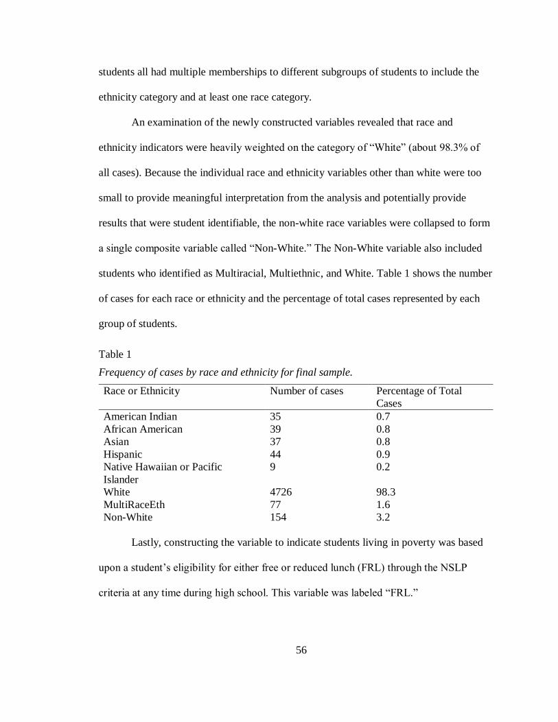
56
students all had multiple memberships to different subgroups of students to include the
ethnicity category and at least one race category.
An examination of the newly constructed variables revealed that race and
ethnicity indicators were heavily weighted on the category of “White” (about 98.3% of
all cases). Because the individual race and ethnicity variables other than white were too
small to provide meaningful interpretation from the analysis and potentially provide
results that were student identifiable, the non-white race variables were collapsed to form
a single composite variable called “Non-White.” The Non-White variable also included
students who identified as Multiracial, Multiethnic, and White. Table 1 shows the number
of cases for each race or ethnicity and the percentage of total cases represented by each
group of students.
Table 1
Frequency of cases by race and ethnicity for final sample.
Race or Ethnicity Number of cases Percentage of Total
Cases
American Indian 35 0.7
African American 39 0.8
Asian 37 0.8
Hispanic 44 0.9
Native Hawaiian or Pacific
Islander
9 0.2
White 4726 98.3
MultiRaceEth 77 1.6
Non-White 154 3.2
Lastly, constructing the variable to indicate students living in poverty was based
upon a student’s eligibility for either free or reduced lunch (FRL) through the NSLP
criteria at any time during high school. This variable was labeled “FRL.”

57
Academic Factors and Variables
Research on college persistence and completion has consistently shown that
academic readiness for college is a predictor of college persistence and completion
(Braxton et al., 2014; Hall, et al., 2008; Hoffman & Lowitzki, 2005; Stumpf & Stanley,
2002; Tinto, 1975; Tinto, 1993; St. John et al., 2000). Vincent Tinto’s theories of student
departure emphasized the importance of separating the domains of academic integration
versus social integration into higher education when examining factors leading to college
persistence (1995).
Variables constructed to measure student’ academic readiness for college
included the scores on the mathematics, reading, and writing sections of the College
Board SAT and the reading and mathematics section of the NECAP. The SAT has been
used as a nationally recognized predictor of college success in many studies and is
frequently used for college admissions (College Board, 2015; Hoffman & Lowitzki,
2005; Niu & Tienda, 2013). The NECAP was designed for use in a small number of
states to measure math and reading skills at grade level according to state achievement
standards as required by No Child Left Behind, the federal education act guiding student
assessment when this study’s students were in high school (Vermont Agency of
Education, 2015a).
When using SAT scores for educational research that predicts success in college,
the College Board recommends using the SAT in conjunction with high school grade
point average (GPA) as a measure of academic readiness (Shaw, 2015). Although, high
school transcript information was not available for this study, validity studies measuring
the relationship between SAT scores and college retention demonstrated that higher SAT

58
composite scores show an increased college retention and graduation rates, even when
controlling for high school GPA (Shaw, 2015). Little research has been conducted on the
relationship between the NECAP and college readiness; however, the assessment is
recognized as an accurate and reportable measure of grade level knowledge and skills for
the subject areas of mathematics, reading and science (Vermont Agency of Education,
2015a; Vermont Agency of Education, 2015c).
An initial exploration of the data revealed cases with duplicate scores for both
NECAP (23 cases) and SAT (1946 cases). The duplicate cases with NECAP scores were
deleted because all score values were the same for each duplicate case.1 The most recent
SAT score was retained for the analysis, which is a method used in other research of SAT
scores predicting success in college (Mattern & Patterson, 2009; Zwick & Himelfarb,
2011).
A bivariate correlation was conducted on the scores for all subject areas in each
assessment. The results showed that SAT Verbal, Math, and Writing scores had strong
relationships between each of the subject areas, therefore not all of the assessment
variables will be used for the analysis. To reduce the likelihood of collinearity among
variables in the multi-level model, the SAT Verbal, Math, and Writing scores were
combined to create a single SAT composite score (Shaw, 2015). The composite SAT
score was then standardized as a Z score to create the continuous variable of academic
1 There were high correlations between NECAP Reading and Math scores with SAT scores, which
prompted a decision to limit assessment variables from the analysis (see Appendix CAppendix D for
Spearman Correlation Matrix of Variables). Further exploration of the data revealed that no students took
the 11th grade NECAP in 2008, so approximately 1/3 of the data was missing (missing values will be
discussed in further detail in the section titled Missing Values). Therefore, the NECAP scores were
removed from the analysis.

59
readiness (variable code label ZSATVERBMATHWRIT). The mean, range, median, and
number of cases for the standardized composite SAT score without missing values can be
found in Table 2, and a histogram showing the distribution of score is in Figure 1.
Table 2
Descriptive statistics for standardized composite SAT scores.
Variable Mean Minimum Maximum Median Valid
Composite SAT Score 0 (0.02) -3.61 3.13 -0.03 3908 (81.3%)
Figure 1. Histogram of standardized composite SAT scores.
60
Family Postsecondary Factors
Variables constructed to measure student factors related family post-secondary
characteristics were collected from results of the Vermont Senior Survey by VSAC. For
the purposes of this study, the Vermont Senior Survey data included a statewide
representation of students who were seniors and graduated in the years 2008, 2010, and
2012. The survey was voluntary, and the annual statewide response rate was
approximately 85% (VSAC, 2015), though many surveys had unanswered questions,
creating missing data. In total, 18,467 surveys were completed and included in the data
set for the study.
For the purposes of this study, survey questions were identified that the
literature suggested could influence college persistence or college completion due to their
relationship to college planning and family education (Braxton et al., 2014; Stage &
Hossler, 1988; Yan, 2002). Answers to survey questions were transformed to become
binary variables. The variables were parent education level, post-secondary planning at
an early age, and serious concerns about paying for college. See Appendix E for a list and
description of the variables created.
Chi-squared tests were conducted to test for collinearity between variables
constructed from survey responses and demographic variables with conceptual or
theoretical constructs that may be similar. The dichotomous variables measured were
Mother has a College Degree, Father has a College Degree, Major Concern about Paying
for College, FRL, and Early Planning. The results of the chi-square tabulation showed
expected counts that were close to actual counts for students with the same value for each
variable, which was an indicator of potential collinearity. The researcher retained the

61
variables Early Planning and FRL for the analysis because these variables have been used
in other studies of college enrollment, persistence and completion (Alarcon & Edwards,
2013; Bowen et al., 2009; Ishitani, 2006; Tinto, 1993). Both variables Mother has a
College Degree and Father has a College Degree were replaced by the variable First
Generation College (PARENTSNODEGREE) to provide an estimate of first generation
college going and parent education level (Ishitani, 2006). Figure 2 shows survey
questions and response options, the newly constructed variables titles, and each variables
respective values derived from the original survey responses.
Survey Questions Constructed Variable Description of Values
What is the highest level of education that
parent(s) or guardian(s) completed?
Mother and Father responses available.
1. Did not finish high school
2. High School diploma or GED
3. Some college or one year certificate
4. 2-year college degree
(associate’s)
5. 4-year college degree (bachelor’s)
6. Master’s, doctorate, or
professional degree
7. Don’t know
First Generation College
(PARENTSNODEGREE)
This dichotomous variable is
a measure of parents’
education level; 1=both
parents have an education
level of less than a college
degree, 0=One or both parents have any type of
college degree (associates,
bachelor, master, doctorate,
or professional degree,
System Missing= no reported
response or “Don’t know”
When did you begin to talk with your
parent(s) or guardian(s) about what to do
after high school?
(Please mark only one.)
Sixth grade or earlier (1) Seventh grade (2)
Eighth grade (3)
Ninth grade (4)
Tenth grade (5)
Eleventh grade (6)
Twelfth grade (7)
I haven’t talked with my
parent(s)/guardian(s) about my plans (8)
Early Planning
(EARLYTALK)
This dichotomous variable
indicates whether a student
talked about their plans after
high school in eighth grade or
earlier. 1=Began to talk about what to do after high school
in grade 8, 7 ,6 or earlier;
0=Began to talk about what
to do after high school in
grade 9, 10, 11, 12 or not at
all.
Figure 2. Survey questions with response options, newly constructed variable titles with
codes, and descriptions of constructed variable values.
62
Selecting the Final Student Variables
Selecting the final student variables for the multilevel model required tests to
determine whether the variables are independent and do not have correlated errors
(Raudenbush & Bryk, 2002). The researcher then used SPSS to perform an OLS with
collinearity diagnostics on 11th grade NECAP reading scores with the following
explanatory variables: Female, Early Planning, FRL, First Generation College,
Composite SAT Score, American Indian, Asian, White, African American, Hispanic,
Hawaiian-Pacific Islander (HawaiiPacific), and Multi Race/Ethnicity. All variables for
race and ethnicity, except Hawaiian-Pacific Islander, had a tolerance of 0.1 or lower and
variance inflation factors (VIF) greater than eight (see Appendix F) signaling the
potential for multi-collinearity (SPSS Web Books-Regression with SPSS, 2016).
A second OLS on 11th grade NECAP reading scores was performed by
including Non-White and excluding all other race and ethnicity variables. The results of
this analysis showed all tolerance coefficients to be greater than 0.8 and the VIF to be
less than two. The level one student variables selected for the model were Female, Non-
White, FRL, Composite SAT Score, Early Planning, and First Generation College.
In summary, the student background and demographic factors included in this analysis
are described in the bullets below with the code title in parenthesis:
Gender-Female (Female)
Race and ethnicity other than White- Non-White (NotWhite)
National School Lunch Program (NSLP) eligibility- Low family income (FRL)
Standardized composite score for College Board SAT Verbal, Mathematics and
Writing sections- Composite SAT Score (ZSATVERBMATHWRIT)
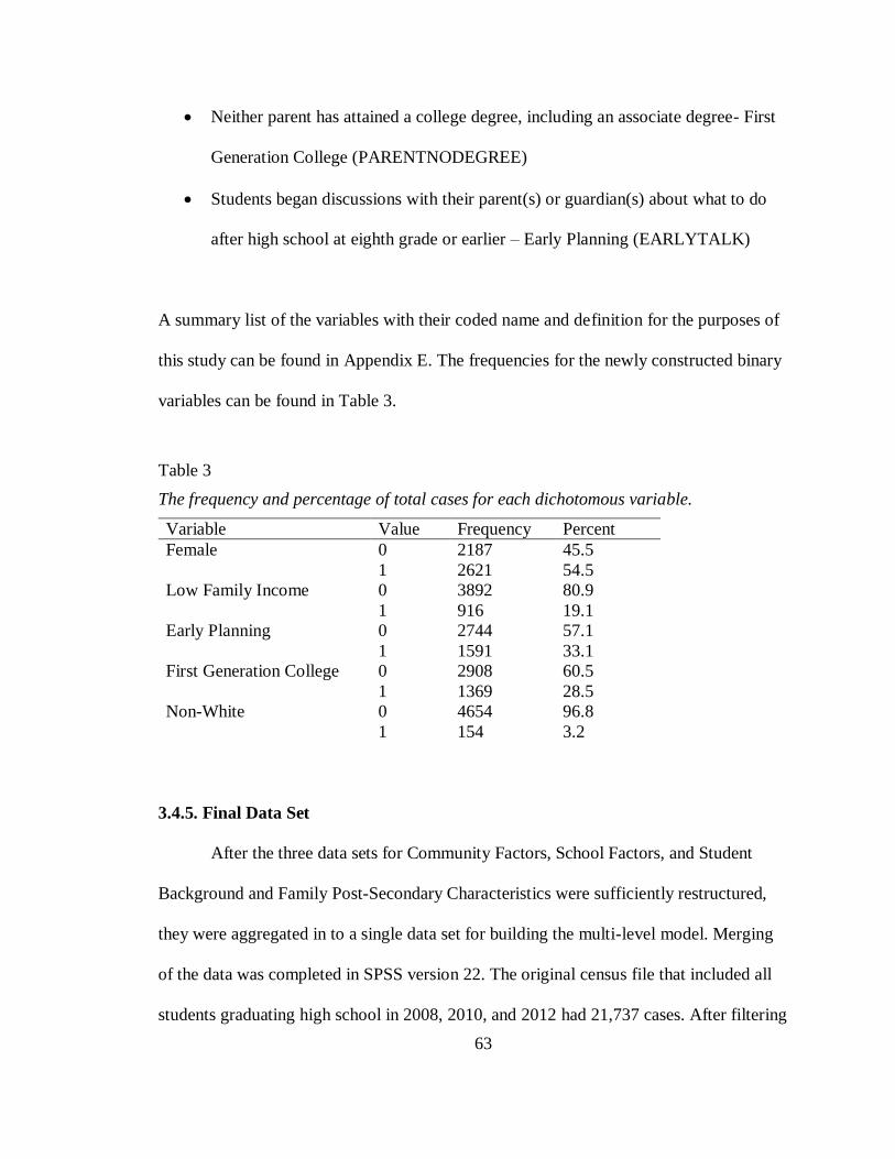
63
Neither parent has attained a college degree, including an associate degree- First
Generation College (PARENTNODEGREE)
Students began discussions with their parent(s) or guardian(s) about what to do
after high school at eighth grade or earlier – Early Planning (EARLYTALK)
A summary list of the variables with their coded name and definition for the purposes of
this study can be found in Appendix E. The frequencies for the newly constructed binary
variables can be found in Table 3.
Table 3
The frequency and percentage of total cases for each dichotomous variable.
Variable Value Frequency Percent
Female 0 2187 45.5
1 2621 54.5
Low Family Income 0 3892 80.9
1 916 19.1
Early Planning 0 2744 57.1
1 1591 33.1
First Generation College 0 2908 60.5
1 1369 28.5
Non-White 0 4654 96.8
1 154 3.2
3.4.5. Final Data Set
After the three data sets for Community Factors, School Factors, and Student
Background and Family Post-Secondary Characteristics were sufficiently restructured,
they were aggregated in to a single data set for building the multi-level model. Merging
of the data was completed in SPSS version 22. The original census file that included all
students graduating high school in 2008, 2010, and 2012 had 21,737 cases. After filtering
64
the data set to only include students who enrolled in the fall semester after graduating
from high school and entered a four-year residential college, 8970 cases remained.
Lastly, the final filtering of data only included students from rural towns who enrolled in
a four-year residential college the fall after graduating from high school and completed
the Vermont Senior Survey. The final data set for the analysis had 4,808 cases.
3.4.6. Construction of the Dependent Variable: College Persistence
Constructing the dependent variable “College Persistence” required extensive data
management from the records retrieved through the NSC. A measurement of consecutive
enrollment in a post-secondary institution for up to two years did not already exist.
Additionally, the wide variety of academic calendars and enrollment terms for post-
secondary institutions in the data provided substantial obstacles for capturing a measure
of continuous enrollment in semesters, trimesters, quarters, summer short-terms, or other
academic schedules. Therefore, the researcher designed a new measure of continuous
enrollment to classify enrollment terms as occurring in either the fall or spring academic
calendar.
To create this measure, the beginning dates of enrollment terms were transformed
into indicators of calendar year quarters by the year of enrollment (e.g., enrollment begin
date for a term in September, 2009 becomes Fall2009). Next, the order, or sequential
placement, of each enrollment term was combined with the calendar year quarter to
provide a reference point of when a student was enrolled during a fall or spring academic
term. For example, if a 2008 high school graduate enrolled in a course at any post-
secondary institution from December 2008 through March, 2009, and it was their second
65
or third enrollment term, it would be included with the variable labeled
EnrollBeginSpring2009.
As the newly created enrollment indicator captured student enrollment into the
spring of their second school year, the formula was expanded to include students who
took summer courses or enrolled at institutions with shorter enrollment terms (e.g.,
trimesters, quarters) so they would be included with their peers enrolled in semester
academic schedules. To control for this growing disparity of ordered or sequential
enrollment terms, the researcher expanded the possible combinations of eligible
enrollment terms for each quarter and year. The formula was analyzed throughout its
development by comparing results of the new variable with individual outlier student
cases in data set. For example, students would be counted as continuously enrolled if they
attended a college with a quarter system and took summer classes or if they attended
sequential semesters and no summer courses.
Following the creation of the enrollment indicator by academic calendar, the
researcher created a variable identifying the Office of Postsecondary Education
Identification (OPEID) code for the institution where each student enrolled in their first
fall season and spring of their last academic season. The OPEID is a code developed by
NCES to “identify schools that have Program Participation Agreements so that its
students are eligible to participate in Federal Student Financial Assistance programs
under Title IV regulations” (NCES, 2015d). If the institution code matched for those two
term periods, the student was identified as having completed two years of post-secondary
education (variable label for 2008 graduates= OPEIDFall08Spring2010). Lastly, all
variables for the three cohorts of students were combined to create a single variable

66
indicating college persistence for four fall and spring academic, or calendar, quarters. See
Appendix G for the SPSS syntax showing the complete formula.
3.5. Missing Values
Several variables in the final data set contained missing values that needed to be
managed before building the multi-level model. Although many of the data sets were
cleaned extensively prior to the researcher’s access, certain data sets had suppressed
values or data missing from the original collection for a variety of reasons. Steps were
taken to identify the scope of missing values and decide how to proceed with filling in
missing data points.
To gain a better understanding of the scope of missing data, the researcher
conducted a missing values analysis in SPSS. The missing values analysis revealed
several variables with missing data points (Table 4).
Table 4
Summary of variables with missing values
Variable N Count Missing Count Percentage
Female 4808 0 0
Low Family Income 4808 0 0
Non-White 4808 0 0
Composite SAT Score 3908 900 18.7
Early Planning 4335 473 9.8
First Generation
College
4277 531 11
The variables constructed from items on the Vermont Senior Survey had a
substantial number of missing results. The variable Early Planning had 9.8% of cases
missing values and First Generation College had 11%. The values were considered
67
missing at random (MAR) due to the incomplete responses on the voluntary survey
(Snijders & Bosker, 2012).
The last category of variables with missing values were the SAT scores, where the
Verbal, Mathematics, and Writing variables each have 900 missing values, or 18.7% of
the cases. When reviewing the SAT data, the missing values were distributed among
students of different high schools, post-secondary institutions, graduation years, gender,
NSLP eligibility, and town of residence. The possible reasons for the missing SAT values
are that students took the SAT in a year other than what was included in the data set for
the analysis or the student did not take the SAT at all. Therefore, it is likely that these
missing scores are MAR (Snijders & Bosker, 2012).
The missing values for group variables were limited to the school level data. All
of the missing values are within the variable Schoolwide College Preparation and only
apply to three schools. The schools with missing values had small student bodies, and
their values were suppressed by the College Board and Vermont Agency of Education in
the publicly available data set as a way to preserve student confidentiality. These missing
values are NMAR. Because there are only 65 cases in the three schools, mean
substitution was used to impute the missing values (Acock, 2005).
The pattern and breadth of missing data was addressed before further analyses
were conducted on the research questions. A statistical method called multiple imputation
was used to make valid inferences on estimations of what values should be imputed
where data is missing (Schafer & Olsen, 1998; Van Buuren, 2007). Imputing values will
yield a complete data set that preserves the structure of the data. Two challenges for
imputation the researcher faced were the classifications of data as MAR and NMAR and

68
the multilevel structure of the data set, where data with missing values are nested within
groups (Snijders & Bosker, 2012). Multiple imputation would be used to replace missing
values of control variables for the final model, but not for any community type
explanatory variables. Before imputing missing values, tests for collinearity were
performed to identify variables that should be excluded from the analysis because
multilevel models are sensitive to variables with strong relationships (Raudenbush &
Bryk, 2002; Snijders & Bosker, 2012).
3.5.1. Multiple Imputation Methodology
The missing values for the data set were addressed through multiple imputation
by chained equations (MICE) or what Van Buuren (2007) called fully conditional
specifications (FCS). The MICE or FCS method builds separate models for each variable
missing data that is conditional on its distribution with all other variables, but does not
require the “simultaneous distribution of all variables jointly” (Snijders & Bosker, 2012,
p. 145; StataCorp, 2015). This method is ideal for the missing data in this analysis
because, as Van Buuren (2007) describes, FCS provides great flexibility to “specify
models that are outside any known standard multivariate density” and maintain
constraints between individual variables (p. 227).
The imputation model was built in Stata using commands specified in Stata
Multiple Imputation Reference Manual 14 (StataCorp, 2015). The Stata commands for
the multiple imputation can be found in Appendix H. The registered imputed variables
were Composite SAT Score, First Generation College, Early Planning, School and Town.
Although there were no missing values for School and Town, they were included as
imputed variables for the analysis to account for clustering within schools and towns. All
69
of the remaining variables were registered as regular variables, including the outcome
variable College Persistence. The imputation model regressed Composite SAT Score,
School, Town and performed a logit with First Generation College and Early Planning.
The independent variables selected were based on their conceptual capacity to represent
relevant student factors but would also not be a perfect predictor. The dependent variable
was also included as an independent variable. A total of 20 imputations were run with a
burn-in period of 10 iterations, which is the recommended number of imputations when
less than 20% of cases have values missing (White, Royston, & Wood, 2011).
3.6. Associations of Group Variables
Before choosing which type of multilevel model to build, the fit between the
groups for towns and schools had to be analyzed for the strength of their association. The
structure of the data implied an imperfect hierarchy of students being members of both
towns and schools, which means that there is not a direct or complete association
between town groups and school groups. To better understand the relationship between
the two sets of groups, the researcher ran a chi square test for association using crosstabs
in SPSS of directional and symmetric measures for nominal by nominal relationships.
The results of the directional measures showed a Lambda value for school dependent
relationships as 0.946 and an uncertainty coefficient of 0.964. The symmetric measures
for Cramer’s V showed a values of 0.908 and a Contingency Coefficient of 0.99. All
results of the analysis were significant and showed a strong association between town and
school groups, which suggests that a two level hierarchical logistic model would likely be
a better model fit rather than a cross-classified model (Britton, 2011; Snijders & Bosker,
2012).
70
CHAPTER 4: RESULTS
This study was designed to measure the likelihood of students from different
kinds of rural communities persisting in college, while controlling for several student and
high school factors that are known to influence college persistence and completion. The
two level hierarchical logistic model was built in stages to address each research
question. First, frequencies for each of the variables were calculated for rural students
who did persist in college and students who did not persist. Second, the empty model was
developed to estimate the group dependent probabilities (Snijders & Bosker, 2012). Then,
parameter estimates for student (level 1) variables were calculated for the likelihood to
persist in college. Next, the level two school variables were added to the model to control
for the random effects for factors attributed the high school. Lastly, interactions between
the type of towns and significant student characteristics were conducted. Each research
question is addressed in the following sections.
4.1. Key Findings for Research Question 1
Research Question: How does college persistence differ among students with different
demographic, socioeconomic, and academic backgrounds across all types of rural
communities and high schools?
4.1.1. Frequency and Distribution Analysis of Variables
Answering the first research question required a descriptive analysis of the
frequency and distribution of the student background and demographic variables as well
as an examination of their association with college persistence (Raudenbush & Bryk,
2002). First, crosstabs were used to provide a count of the values for binary variables for
the two student groups: “persistors” and “non-persistors”. The results of the frequencies
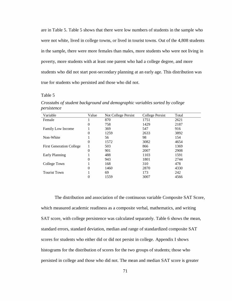
71
are in Table 5. Table 5 shows that there were low numbers of students in the sample who
were not white, lived in college towns, or lived in tourist towns. Out of the 4,808 students
in the sample, there were more females than males, more students who were not living in
poverty, more students with at least one parent who had a college degree, and more
students who did not start post-secondary planning at an early age. This distribution was
true for students who persisted and those who did not.
Table 5
Crosstabs of student background and demographic variables sorted by college
persistence
Variable Value Not College Persist College Persist Total
Female 1 870 1751 2621
0 758 1429 2187 Family Low Income 1 369 547 916
0 1259 2633 3892
Non-White 1 56 98 154
0 1572 3082 4654
First Generation College 1 503 866 1369
0 901 2007 2908
Early Planning 1 488 1103 1591
0 943 1801 2744
College Town 1 168 310 478
0 1460 2870 4330
Tourist Town 1 69 173 242 0 1559 3007 4566
The distribution and association of the continuous variable Composite SAT Score,
which measured academic readiness as a composite verbal, mathematics, and writing
SAT score, with college persistence was calculated separately. Table 6 shows the mean,
standard errors, standard deviation, median and range of standardized composite SAT
scores for students who either did or did not persist in college. Appendix I shows
histograms for the distribution of scores for the two groups of students; those who
persisted in college and those who did not. The mean and median SAT score is greater
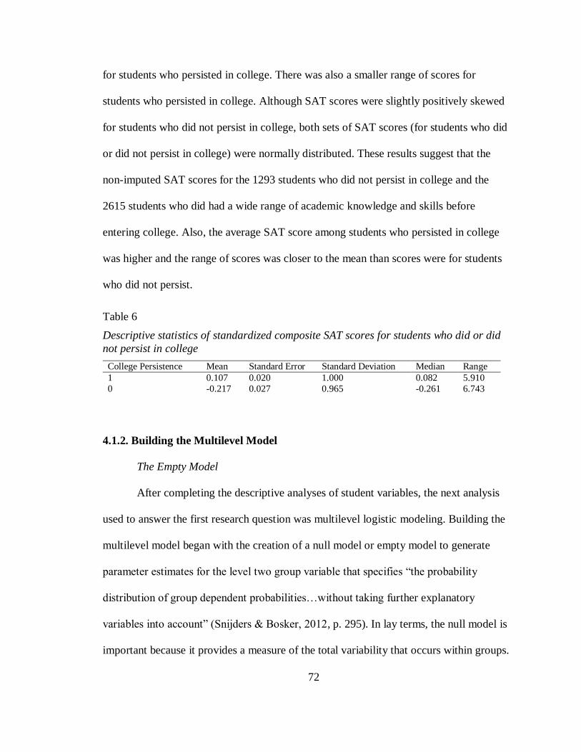
72
for students who persisted in college. There was also a smaller range of scores for
students who persisted in college. Although SAT scores were slightly positively skewed
for students who did not persist in college, both sets of SAT scores (for students who did
or did not persist in college) were normally distributed. These results suggest that the
non-imputed SAT scores for the 1293 students who did not persist in college and the
2615 students who did had a wide range of academic knowledge and skills before
entering college. Also, the average SAT score among students who persisted in college
was higher and the range of scores was closer to the mean than scores were for students
who did not persist.
Table 6
Descriptive statistics of standardized composite SAT scores for students who did or did
not persist in college
College Persistence Mean Standard Error Standard Deviation Median Range
1 0.107 0.020 1.000 0.082 5.910
0 -0.217 0.027 0.965 -0.261 6.743
4.1.2. Building the Multilevel Model
The Empty Model
After completing the descriptive analyses of student variables, the next analysis
used to answer the first research question was multilevel logistic modeling. Building the
multilevel model began with the creation of a null model or empty model to generate
parameter estimates for the level two group variable that specifies “the probability
distribution of group dependent probabilities…without taking further explanatory
variables into account” (Snijders & Bosker, 2012, p. 295). In lay terms, the null model is
important because it provides a measure of the total variability that occurs within groups.
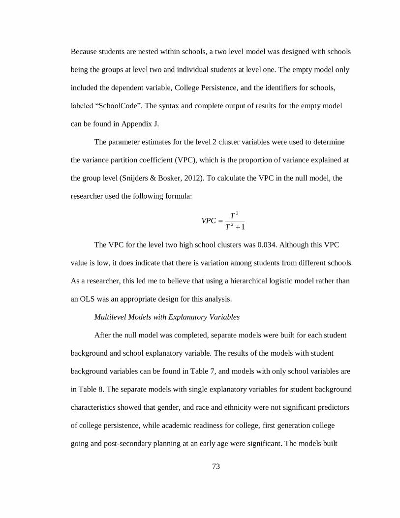
73
Because students are nested within schools, a two level model was designed with schools
being the groups at level two and individual students at level one. The empty model only
included the dependent variable, College Persistence, and the identifiers for schools,
labeled “SchoolCode”. The syntax and complete output of results for the empty model
can be found in Appendix J.
The parameter estimates for the level 2 cluster variables were used to determine
the variance partition coefficient (VPC), which is the proportion of variance explained at
the group level (Snijders & Bosker, 2012). To calculate the VPC in the null model, the
researcher used the following formula:
12
2
T
TVPC
The VPC for the level two high school clusters was 0.034. Although this VPC
value is low, it does indicate that there is variation among students from different schools.
As a researcher, this led me to believe that using a hierarchical logistic model rather than
an OLS was an appropriate design for this analysis.
Multilevel Models with Explanatory Variables
After the null model was completed, separate models were built for each student
background and school explanatory variable. The results of the models with student
background variables can be found in Table 7, and models with only school variables are
in Table 8. The separate models with single explanatory variables for student background
characteristics showed that gender, and race and ethnicity were not significant predictors
of college persistence, while academic readiness for college, first generation college
going and post-secondary planning at an early age were significant. The models built

74
with single variables for school factors showed that schoolwide socioeconomic status was
a significant predictor that students were slightly less likely to persist in college while
schoolwide preparation for college did not show a significant relationship.
Table 7
Parameter Estimates for Multilevel Models with a Single Explanatory Variable for
Student Background Factors on College Persistence
Parameter
Estimate
Female Low Family
Income
Non-White Composite SAT Score First Generation
College
Early Planning
Odds
Ratio
1.07 (0.07) 0.73***
(0.06)
0.89 (0.15) 1.43*** (0.05) 0.79*** (0.05) 1.20*** (0.08)
Constant 1.85***
(0.10)
2.06***
(0.09)
1.93***
(0.08)
2.00*** (0.08) 2.09*** (0.10) 1.80*** (0.09)
Random
Effects
Parameter
Estimate
0.19 (0.05) 0.17 (0.05) 0.19 (0.05) 0.13 (0.06) 0.17 (0.05) 0.19 (0.05)
Notes: *p ≤ 0.10 **p ≤ 0.05 ***p ≤ 0.01 after rounding. Standard errors are in parenthesis
Table 8
Parameter Estimates for Multilevel Models with a Single Explanatory Level 2 Variable
for School Characteristics
Parameter Estimate Schoolwide SES Schoolwide College Preparation
Odds Ratio 0.99*** (0.00) 1.00 (0.00)
Constant 2.45*** (0.25) 1.66*** (0.30)
Random Effects 0.15 (0.05) 0.18 (0.05)
Note: *p ≤ 0.10 **p ≤ 0.05 ***p ≤ 0.01 after rounding Standard errors are in parenthesis
Next, individual student variables were added to the model to estimate the effects
of demographic, academic, and family backgrounds on college persistence. Each of these
explanatory variables was chosen for inclusion in the model due to its well-established
link to persistence (Bowen et al., 2009; Coleman, 1968; Nora, 2004; Tinto, 1975). At
first, the variables indicating student characteristics were added to the model to represent
indicators of gender, low family income, non-white race and ethnicity, and academic
75
readiness for college. Then, two relevant family background characteristic. First
Generation College and Early Planning, were included in the model. The odds ratios for
the variables in each model are reported in column one in Table 9.
Model 1 in Table 9 goes on to show that the student characteristics for gender and
race and ethnicity did not have a significant relationship with college persistence.
However, the surrogate measurement for academic readiness, composite SAT score (odds
ratio 1.41), and low family income (odds ratio 0.92) showed a significant effect. Both of
the variables measuring Family Characteristics, First Generation College and Early
Planning were not significant.
In summary, the results of the multilevel model for student background variables
demographic, academic, and family backgrounds on college persistence show that student
family income status and academic readiness are significant predictors of college
persistence for students from any type of Vermont’s rural communities. Rural students
living in poverty are 0.82 times less likely to persist in a four-year residential college,
while for each unit increase in academic readiness, students are 1.41 times more likely to
persist in college. Although parent post-secondary education and student college planning
at an early age are significant predictors of college persistence, the effects are not
significant when other variables are added to the model. The results of Models 2, 3 and 4
are reported in the Key Findings for Research Questions 2 and 3.
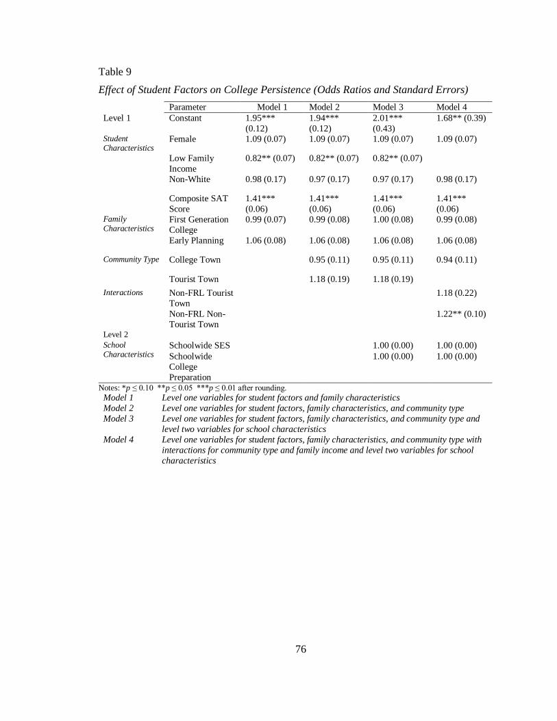
76
Table 9
Effect of Student Factors on College Persistence (Odds Ratios and Standard Errors)
Parameter Model 1 Model 2 Model 3 Model 4
Level 1 Constant 1.95***
(0.12)
1.94***
(0.12)
2.01***
(0.43)
1.68** (0.39)
Student Characteristics
Female 1.09 (0.07) 1.09 (0.07) 1.09 (0.07) 1.09 (0.07)
Low Family
Income
0.82** (0.07) 0.82** (0.07) 0.82** (0.07)
Non-White 0.98 (0.17) 0.97 (0.17) 0.97 (0.17) 0.98 (0.17)
Composite SAT
Score
1.41***
(0.06)
1.41***
(0.06)
1.41***
(0.06)
1.41***
(0.06) Family Characteristics
First Generation
College
0.99 (0.07) 0.99 (0.08) 1.00 (0.08) 0.99 (0.08)
Early Planning 1.06 (0.08) 1.06 (0.08) 1.06 (0.08) 1.06 (0.08)
Community Type College Town 0.95 (0.11) 0.95 (0.11) 0.94 (0.11)
Tourist Town 1.18 (0.19) 1.18 (0.19)
Interactions Non-FRL Tourist
Town
1.18 (0.22)
Non-FRL Non-
Tourist Town
1.22** (0.10)
Level 2 School Characteristics
Schoolwide SES 1.00 (0.00) 1.00 (0.00)
Schoolwide
College
Preparation
1.00 (0.00) 1.00 (0.00)
Notes: *p ≤ 0.10 **p ≤ 0.05 ***p ≤ 0.01 after rounding.
Model 1 Level one variables for student factors and family characteristics
Model 2 Level one variables for student factors, family characteristics, and community type
Model 3 Level one variables for student factors, family characteristics, and community type and
level two variables for school characteristics
Model 4 Level one variables for student factors, family characteristics, and community type with
interactions for community type and family income and level two variables for school
characteristics
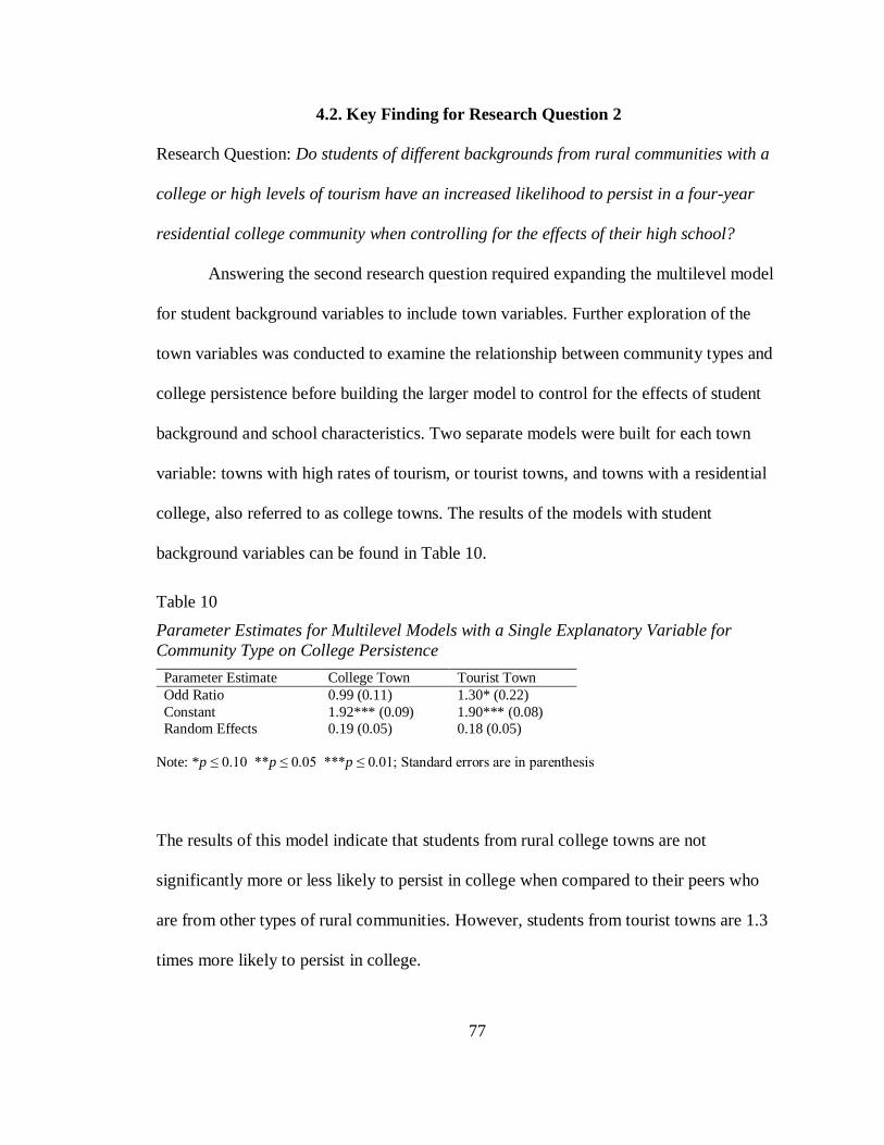
77
4.2. Key Finding for Research Question 2
Research Question: Do students of different backgrounds from rural communities with a
college or high levels of tourism have an increased likelihood to persist in a four-year
residential college community when controlling for the effects of their high school?
Answering the second research question required expanding the multilevel model
for student background variables to include town variables. Further exploration of the
town variables was conducted to examine the relationship between community types and
college persistence before building the larger model to control for the effects of student
background and school characteristics. Two separate models were built for each town
variable: towns with high rates of tourism, or tourist towns, and towns with a residential
college, also referred to as college towns. The results of the models with student
background variables can be found in Table 10.
Table 10
Parameter Estimates for Multilevel Models with a Single Explanatory Variable for
Community Type on College Persistence
Parameter Estimate College Town Tourist Town
Odd Ratio 0.99 (0.11) 1.30* (0.22)
Constant 1.92*** (0.09) 1.90*** (0.08)
Random Effects 0.19 (0.05) 0.18 (0.05)
Note: *p ≤ 0.10 **p ≤ 0.05 ***p ≤ 0.01; Standard errors are in parenthesis
The results of this model indicate that students from rural college towns are not
significantly more or less likely to persist in college when compared to their peers who
are from other types of rural communities. However, students from tourist towns are 1.3
times more likely to persist in college.

78
Next, the researcher expanded the multilevel model by adding variables to control
for the effects of student background factors and school characteristics on college
persistence. Although the only two variables with statistically significant results in the
first model were family income status and academic readiness for college, all of the
student and school variables were included to fit the new model because of their
theoretical importance and statistical independence (or non-collinearity) (Raudenbush &
Bryk, 2002; Snijders & Bosker, 2012). The town level variables indicating tourist towns
and college towns were added to the model at the same time to test the second research
question before controlling for the effects of schools at the second level.
The odds ratios for the variables in each model are reported in Model 2 of Table
9. The newly added variables measuring Community Type were not significant. The
results for Tourist Town and College Town were directional with the hypothesis,
however they were not significant. Similar to Model 1, the student characteristics for
gender and race and ethnicity did not have a significant relationship with college
persistence. Both of the variables measuring Family Characteristics, First Generation
College and Early Planning, were also not significant. The only two variables with
significant effects were composite SAT score (odds ratio 1.41), and low family income
(odds ratio 0.92).
Lastly, to control for the effects high schools have on college persistence and
completion, the researcher created another model by adding explanatory variables to
measure the aggregate socioeconomic status of the school (Schoolwide SES) and the
school-wide college preparation qualities (Schoolwide College Preparation). The odds
ratios for the variables in each model are reported in Model 3 of Table 9. The odds ratios

79
for both Schoolwide SES and Schoolwide College Preparation were not significant.
Similar to Model 2, all of the remaining variables in the model were not significant
except for composite SAT score (odds ratio 1.41), and low family income (odds ratio
0.92).
The second key finding of this study is that the effects associated with living in a
rural tourist town or college town does not in itself show a significant impact on a
student’s ability to successfully transition into a college community. The effect of a
student’s home community did not substantially impact the transition into college when
accounting for factors related to a student’s academic readiness, family income, first
generation college going, post-secondary planning at an early age, race/ethnicity, and
high school socioeconomic status and college preparation. Although tourist towns did
show an increased likelihood for college persistence when no other control variables were
added to the model (odd ratio 1.30, p=0.11), both the odds ratio and significance of the
parameter estimates changed after adding control variables (see Appendix K). After all
control variables were added to the model, the slight increase in the likelihood of college
persistence for students from tourist towns was not significant. The odds ratio for
students from a college town to persist in college actually showed a reduced likelihood
and was also not statistically significant.
The results of the analysis indicate that student variables measuring non-White
race and ethnicity, gender, first generation college going, and post-secondary planning at
an early age have no significant effect on persistence at a four-year residential college.
However, the measure of academic readiness (Composite SAT Score) and low family
income continue to show a significant relationship with college persistence. For every
80
one-point increase in the standardized composite SAT score, students are 1.41 times more
likely to persist in college. Students who are members of low-income households are 0.82
times less likely to persist in college.
4.3. Key Finding for Research Question 3
Research Question: How does college persistence differ among students in tourist towns
with different demographic, socioeconomic, and academic backgrounds?
The third research question is a closer examination of the background variables
for students from tourist towns to see if community factors have a different effect
between students in tourist communities. Answering the third research question required
two steps. First, a descriptive analysis of the student factors for students from rural tourist
communities was required to identify the appropriate variables for fitting a multilevel
model. Second, a fourth multilevel model was built to measure the interaction between
student background variables and rural tourist communities. Selecting the student
demographic and socioeconomic background variables for the multilevel model was
based on the results of the multilevel built for question two and the descriptive analysis of
student background characteristics in tourist towns. The purpose of conducting these
interactions is to better understand any differences in college persistence related to family
income, the only non-academic student background variable shown to be significant in
the previous three models, which may also be associated with community type.
However, there was no significant difference between students from tourist towns not
living in poverty when compared to their peers from other rural communities.

81
The results of research question three show that family income status was the only
demographic or family background variable to have a significant relationship with
college persistence. Fitting a model with an interaction of family income status with
tourist town was not possible because of high standard errors in the results, which may
have been due to the small number of students who were from low income families and
lived in tourist towns. However, specifying student family income as above the poverty
measure allowed for the use of two newly constructed interaction variables for non-FRL
Tourist Town and non-FRL non-Tourist Town. These two interaction variables were
created as dummy variables to measure the interaction between family income status and
tourist town. The variables for FRL and Tourist Town were not included in the fourth
model to prevent collinearity. The odds ratios for the variables in the fourth and final
model are reported in Model 4 on Table 9.
In Model 4, family financial status proved to be a greater predictor of college
persistence than community effects when the interaction between students living in
poverty and the tourism community indicator was unpacked using an interaction. Income
status had a significant interaction with students from non-tourist towns. Students not
living in poverty were 1.22 times more likely to persist in college. To examine this
finding further, a crosstabs analysis was conducted on the non-imputed data set to
measure the number of students in tourist towns and non-tourist towns according to their
individual and family characteristics. The results of this analysis can be found in Table
11, which shows the number of students for each combination of student background
factors in Tourist Town and non-Tourist Town communities. The percentage of students
from the sample in tourist towns was also calculated for each background variable.
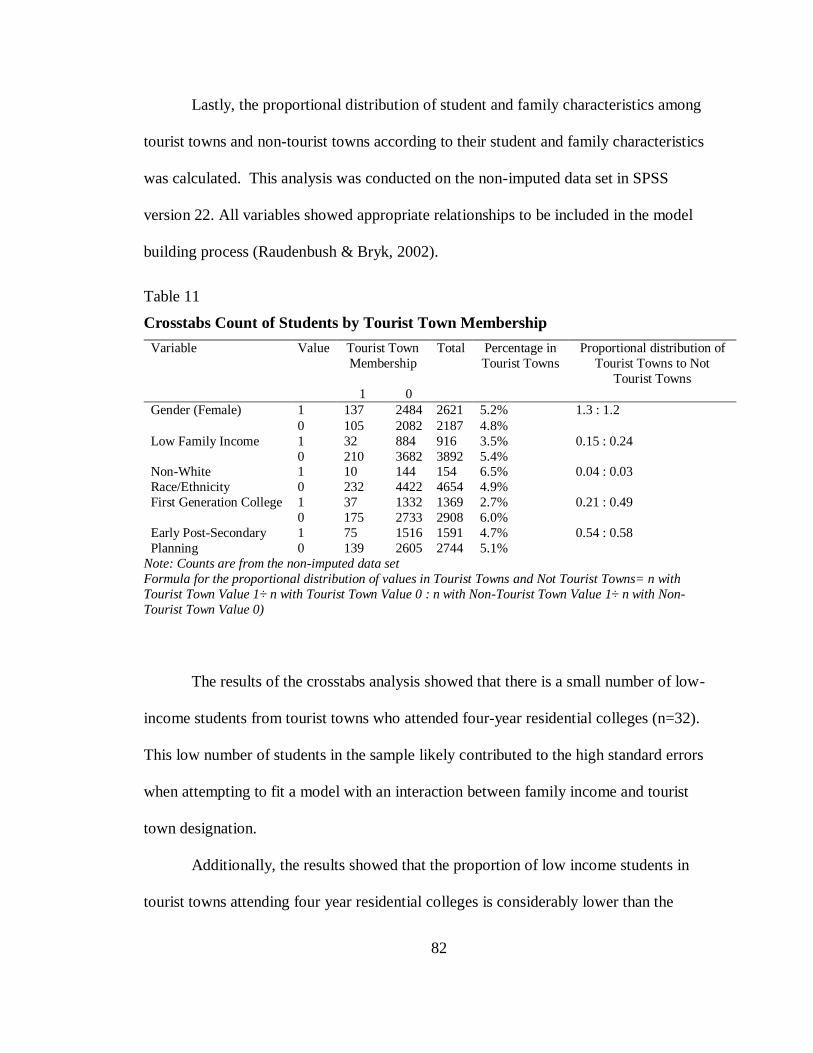
82
Lastly, the proportional distribution of student and family characteristics among
tourist towns and non-tourist towns according to their student and family characteristics
was calculated. This analysis was conducted on the non-imputed data set in SPSS
version 22. All variables showed appropriate relationships to be included in the model
building process (Raudenbush & Bryk, 2002).
Table 11
Crosstabs Count of Students by Tourist Town Membership
Variable Value Tourist Town
Membership
Total Percentage in
Tourist Towns
Proportional distribution of
Tourist Towns to Not
Tourist Towns
1 0
Gender (Female) 1 137 2484 2621 5.2% 1.3 : 1.2
0 105 2082 2187 4.8%
Low Family Income 1 32 884 916 3.5% 0.15 : 0.24
0 210 3682 3892 5.4% Non-White
Race/Ethnicity
1 10 144 154 6.5% 0.04 : 0.03
0 232 4422 4654 4.9%
First Generation College 1 37 1332 1369 2.7% 0.21 : 0.49
0 175 2733 2908 6.0%
Early Post-Secondary
Planning
1 75 1516 1591 4.7% 0.54 : 0.58
0 139 2605 2744 5.1%
Note: Counts are from the non-imputed data set
Formula for the proportional distribution of values in Tourist Towns and Not Tourist Towns= n with
Tourist Town Value 1÷ n with Tourist Town Value 0 : n with Non-Tourist Town Value 1÷ n with Non-
Tourist Town Value 0)
The results of the crosstabs analysis showed that there is a small number of low-
income students from tourist towns who attended four-year residential colleges (n=32).
This low number of students in the sample likely contributed to the high standard errors
when attempting to fit a model with an interaction between family income and tourist
town designation.
Additionally, the results showed that the proportion of low income students in
tourist towns attending four year residential colleges is considerably lower than the
83
proportion of low income students from non-tourist communities. Moreover, when
looking at the subgroup of First Generation College students, there are proportionally
fewer students in tourist towns than in non-tourist towns. These two results suggest that
the socioeconomic status and parent education level is generally higher for families of
four-year college-going students from tourist communities than other rural communities.
84
CHAPTER 5: DISCUSSION
This study sought to examine whether students from a variety of rural
communities substantively different in their attendance and persistence in college.
According to Vincent Tinto’s interactionalist theory of departure from higher education,
students who persist in college are able to successfully complete three stages: separation
from past associations, transition between high school and college, and incorporate into
the new society of college (Tinto, 1993). This study analyzed whether the factors of a
rural tourist town or college community supported cultural capital development that
would increase the likelihood of students having a successful incorporation into the
academic and social systems of college.
Tourists visiting rural communities from outside of the local area bring with them
behaviors and physical property of a different culture (e.g., automobiles, clothing,
recreational equipment, and personal technology devices). The kind of social and cultural
contributions tourists bring with them to a rural community allows local residents to be
exposed to behaviors, social trends, and lifestyles that may not otherwise be experienced
in their local community (Deery et al., 2011; Dogan, 1989; Gossling, 2002).
Additionally, colleges also shape the social, cultural, and economic character of a
rural community (Gumprecht, 2003; Smallwood, 1971; Weill, 2009). The presence of a
college introduces spending that supports the local economy, provides additional public
space for intellectual pursuits or recreation, and potentially a more racially or ethnically
diverse population to the local community (Gumprecht, 2003; Gumprecht 2007; Massey
et al., 2014; Weill, 2009).
85
This study posits that students from tourist communities develop a cultural capital
and habitus through exposure to frequent non-residential tourist behaviors and properties
that would support their adjustment to the social and physical environment of a
residential four-year college. Likewise, students exposed to the activities and physical
presence of a residential college campus in a rural community are likely to become
familiar with the variety of people and behaviors they may encounter during a college
experience (Sage & Sherman, 2014), similarly easing their transition into college.
Multilevel logistic modeling was used to test the hypothesis that students who
complete secondary school in a rural community with a substantial presence of non-
residential tourists or a college within their residential community show an increased
likelihood of persisting in college for at least two years after initial enrollment. Using a
data set constructed from multiple sources, several explanatory variables were used in the
model to control for the effects high schools and student background characteristics on
college persistence. The findings of this study provide insight to Vincent Tinto’s (1993)
interactionalist theory of departure from higher education as it relates to students from
different types of rural communities.
5.1. Discussion of Findings for Research Question 1
How does college persistence differ among students with different demographic,
socioeconomic, and academic backgrounds across all types of rural communities and
high schools?
The key finding for this research question showed that student family income
status and academic readiness are significant predictors of college persistence for
students from rural communities. Although first generation college going and college
86
planning at an early age were significant predictors of college persistence, the effects
were not significant when other variables were added to the model. There was no
significant difference in college persistence according to gender or race and ethnicity
when the variables were used as a predictor in a single variable model or when included
with other student variables in a multilevel model. This finding further emphasizes the
literature outlining the importance of family financial status and academic readiness for
college as critical factors that influence college persistence and completion (Bowen et al.,
2009; Braxton et al., 2014; Niu & Tienda, 2013; Nora, 2004; Tinto, 1993).
There are several possible reasons for the statistically non-significant relationship
of certain variables with college persistence. First, the likely reason for why the race and
ethnicity variable was not a significant factor in this study is that the number of students
in the sample was too small. The sample size for this study was not large enough to find
an effect, even after aggregating students of racial and ethnic backgrounds known to be
related with persistence gaps into a single variable of Non-White (Bowen et al., 2014).
Second, variables such as post-secondary planning at an early age and first generation
college going likely lost their significance when other related student factors, such as
poverty, with stronger predictive power were included in the model. This finding is
congruent with previous studies suggesting that family income plays a stronger role in
graduating on time than parental education (Bowen et al., 2014). Also, it has been
established that low family income has a strong relationship with post-secondary
planning at an early age and college degree attainment in parents (Hill & Wang, 2015;
Stage & Hossler, 1988; Yan, 2002). The presence of this relationship was also shown in
the correlation matrix in Appendix D.
87
5.2. Discussion of Findings for Research Question 2
Do students from rural communities with a college or high levels of tourism have a
greater likelihood to persist in a four-year residential college community when
controlling for the effects of their high school?
The multilevel models fit with only one variable did show a significant
relationship for all variables except gender, race and ethnicity, college town, and
schoolwide college preparation. However, after all the predictor variables were then
added to the model as control variables for community type, the two variables that
remained statistically significant were low family income and academic readiness.
Community type was not statistically significant for tourist towns or college towns.
This finding builds upon the literature exploring college going tendencies for rural
students and the relationship between the distance a rural student lives from a college and
their educational choices (Sage & Sherman, 2014; Turley 2009). Turley (2009) found a
small but significant relationship between the distance a student lives from college and
their likelihood to apply and enroll in post-secondary education. One suggested reason
was that the close proximity a student lived to a college provided a convenience
mechanism for separating from home and an emotionally easier transition into college
(Turley, 2009). In this study, college town is also a surrogate measurement for the
distance a student lives from a four-year residential college. The results of this study
show that persisting in any four-year residential college after enrollment is not impacted
by proximity.
Additionally, the non-significant findings for students from tourist communities
suggest that any difference in cultural capital developed by students from tourist
88
communities does not have an impact on college persistence. The factors that contribute
to a student’s successful transition into and retention in a college community are not
directly related to the characteristics of rural tourist communities. The impact of a
student’s socioeconomic status and academic readiness for college plays a greater role in
shaping the cultural capital supporting college persistence than the effects of their home
community. The different physical, social, and cultural structures of tourist and college
communities do not appear to have a significant impact on the development of cultural
capital that relates with factors contributing to college persistence. Therefore, it is likely
that any possible habitus students develop that is unique to tourist or rural college
communities is separate from the effect of socioeconomic status and has little direct
relationship with traits supporting a successful incorporation into a college community.
There is not sufficient evidence from this study to show that a student’s home
rural community influences the social and cultural transition into a college community
such that it has an impact on college persistence. This finding contributes to the existing
research by Tinto (1993) and Nora (2003, 2004) on the effect of pre-college factors on
the transition and integration into a higher education community. As Tinto (1975, 1993)
outlined in his interactionalist theory of departure from higher education, the dispositions
and attributes of a student entering college plays a role in their likelihood to transition
and integrate into a new academic and social community. Furthermore, students from
communities with drastically different norms and behaviors than college life may be at a
disadvantage for persisting (Tinto, 1993). This key finding contributes to Tinto’s theory
by showing that any difference in student dispositions or attributes that may result from

89
living in a rural tourist town or college town during high school does not have a clear
relationship with the transition and incorporation into a college community.
The results also contribute to Nora’s (2004) conceptual framework of
psychosocial factors related to college predispositions, search, choice and reenrollment.
As Nora (2004) explained, the cultural capital and habitus developed from pre-college
experiences plays an important role in a student’s integration into a college community,
the new social network, and feelings of acceptance with the post-secondary institution. In
Nora’s (2003) Student Engagement Model, the category of pre-college psychosocial
factors that help draw students to or pull them away from higher education primarily
include factors related to high school and home environment. These factors can
predispose students to the social experiences and involvement in learning experiences at
post-secondary institutions that lead toward college persistence (Nora, 2003, 2004). The
findings of this study reveal that a student’s membership in a distinct rural community
type is not likely to play a role in the psychosocial factors that significantly relates to
their social experiences along the pathway to re-enrolling and persisting in college.
Specifically, coming from a rural tourist town does not significantly contribute to
experiences related with college persistence.
5.3. Discussion of Findings for Research Question 3
How does college persistence differ among students in tourist towns with different
socioeconomic backgrounds?
Analyzing the interaction between low family income and tourist community type
for this research question was a challenge because of the small number of students in the
sample who were from tourist towns. Out of the 242 students from tourist towns, only 32

90
were from low income families. The size of this small subgroup of the sample likely
contributed to large standard errors for the interaction terms in the multilevel model. The
large standard errors limited the analysis to interactions for students not eligible for free
and reduced lunch.
When analyzing the parameter estimates that were significant and did not have
large standard errors, there was no significant difference for tourist community type and
college persistence among students not eligible for free and reduced lunch.This finding
suggests that there is a non-significant difference in the effects of a rural tourist
community on a student from a low income family that would predict their likelihood to
transition into academic, social, and residential demands of a college community. The
implication of this finding is that efforts made by schools and policy makers to improve
college persistence should focus on the individual student and their assets supporting
their likelihood to succeed in college.
However, it is important to recognize that college persistence is different than
enrollment. It is the researcher’s speculation that the effects of a rural student’s
community on their habitus and sense of place is likely to have a stronger relationship
with a student’s decision to attend and which college they choose to attend rather than
whether or not they persist during the school year. The habitus and sense of place a
student develops from their home community shapes how they see themselves in the
world and is likely to be an important factor in their decision making about where they
would like to be after high school and the social context where they would be
comfortable (Braxton, 2014; Nora, 2004; Tinto, 1987). A student’s anticipation and
preparation for social integration into a new college community is likely to begin well
91
before they arrive on campus and enroll in coursework (Braxton, 2014; Tinto, 1987). To
further test the hypothesis that the cultural capital developed by students living in tourist
communities is different than their college going peers in other rural communities,
additional research can track where students enroll in college to see if there is a
relationship with the characteristics of tourists vising the local community.
As Nora emphasized (2004), the enrollment process includes the decision making
prior to applying and attending college. Students’ habitus and cultural capital play a
substantial role in how a student tries to match themselves with a post-secondary
educational experience. The results of this key finding suggest that future research about
rural community effects on post-secondary education should examine the type of post-
secondary match students make which leads to college persistence. A study of this design
would measure the characteristics of colleges where students of different backgrounds
successfully persisted in college.
5.4. Limitations
The purpose of this study was to examine the relationship between rural tourism
community factors and integration into college according to Tinto’s interactionist theory
of student departure from higher education. There were four major limitations to this
study which may have impacted the findings that fell into two categories: data sampling
and data quality.
Data sampling
The foremost limitation of this study related to data quality was the absence of
direct measurements for the quantity and quality of interactions between students and
tourists. It is likely that students who grew up in a tourist town had very different

92
experiences with tourists visiting their community. The absence of a student or family
measure for the type of interactions and relationships local residents have with tourists
did not allow the study to control for different levels of exposure, or potential influences
or tourism. Additionally, the broad definition of tourist towns as defined by political
boundaries allows for variance in the true experience students would have with tourists.
Second, the sample was only limited to cases in one state within the northern New
England region that had complete data values for all variables in multiple data sets. The
results have the highest degree of relevance for the communities of Vermont and the
Northern New England region, but may not be generalizable to other regions of the US or
other countries. The history of post-secondary institutions and tourism development in
northern New England is unique to this region of the US. Other regions may have a
similar geo-spatial and cultural relationship between urban areas and rural communities,
but that was not tested as part of the analysis.
Additionally, the small size of the tourist community type subgroups within the
sample did not allow for certain analyses. This statistical limitation may have masked
effects that would have been noticeable with a larger sample. Another subgroup with a
small representation in the sample was students with a race or ethnicity other than white,
which the literature has shown is a strong predictor of college persistence (Bowen et al.,
2010). A larger sample with more students representing greater ethnic and racial
diversity, perhaps in a follow up study, would allow for a more detailed analysis of race
and ethnicity as a student factor.
93
Data Quality
The foremost limitation of this study related to data quality was the substantial
number of cases with missing values for composite SAT scores and responses on the
Senior Survey for early college planning and parental college degree. Although the
missing values were determined to be MAR, the actual (non-imputed) representation of
data was notably reduced for these three variables (Snijders & Bosker, 2012). Of
particular emphasis for missing data is the nearly 19% of the cases missing values for
composite SAT score. The composite SAT scores was the only continuous variable in the
model and also the only measure of academic readiness in the models. Moreover, all of
the multilevel models built with composite SAT score showed a significant relationship
for this variable with college persistence. The possible impact for the missing data of
composite SAT score, early college planning, and parental college degree is not known
and could have potentially impacted the results.
Second, the analysis did not control for student behaviors and experiences while
attending college, which are attributed to many of the factors associated with dropping
out of college (Braxton, 2014; Tinto, 1987). The data used for this analysis did not
measure any aspects of the student’s college experience, only their enrollment up to two
years. However, because this measurement of college persistence required continuous
enrollment for at least two years is stricter than many other definitions used in prior
research, this analysis does provide an accurate look at the enrollment indicators that lead
toward college completion (Kahn & Nauta, 2001).
94
5.5. Conclusion
This study sought to measure the likelihood that rural students would persist in
college based on whether they came from a rural community with a college or high rates
of tourism while controlling for several student background factors and school
characteristics. Overall, there was no significant difference in the likelihood to persist in
college among students of different types of rural communities when accounting for
school and student background factors. Consistent with the literature on college
completion, the student background factors of family income and college academic
readiness are the strongest predictors of college persistence.
Efforts made by policy makers to improve rates of college completion for rural
students in northern New England will need to focus on supporting students’ academic
preparation before entering college and overcoming the challenges that living in poverty
presents to persistence. Resources to support rural students who are enrolling in college
should be distributed without concern for the type of rural community where they reside.
Exposing students to college communities should be intentional and structured to provide
a realistic expectation of what life at college will be like, because living in close
proximity to a college is not in itself a reliable mechanism. Academic readiness for
college should include sufficient preparation in mathematics, reading, and writing. This
study suggests supporting the academic and socioeconomic needs for each individual
student is the most effective pathway to improving college persistence and college
completion for rural youth.
95
REFERENCES
Acock, A. C. (2005, November). Working with Missing Values. Journal of Marriage and
Family, 67(4) pp. 1012-1028.
Alarcon, G. M., & Edwards, J. M. (2013). Ability and motivation: Assessing individual
factors that contribute to university retention. Journal of Educational Psychology,
105(1), 129-137.
Andereck, K. L, Valentine, K. M., Knopf, R. C., & Vogt C. A. (2005). Residents'
perceptions of community tourism impacts. Annals of Tourism Research, 32(4)
1056–1076
Andereck, K., Valentine, K., Vogt, C., & Knopf, R. (2007). Across-cultural analysis of
tourism and quality of life perceptions. Journal of Sustainable Tourism, 15(5),
483e502.
Ap, J. (1992). Residents’ perceptions on tourism impacts. Annals of Tourism Research,
19, 665-690.
Arce, W. M., Giles, S., & ZuWallack, R. S. (2009, July). A modified method of
estimating the postsecondary enrollment rates of recent Vermont high school
graduates: Class of 2007 Senior Survey. Vermont Student Assistance
Corporation: Winooski, VT. Retrieved from
http://services.vsac.org/wps/wcm/connect/822811804f52e01e8152b7c73da1011c/
2007SeniorSurvey_ContinuationStudyMethods.pdf?MOD=AJPERES
Arce, W. M. (2015). Discussions with Vermont Student Assistance Corporation
researchers managed and provided data.
Aud, S., Fox, M., & Kewal Ramani, A. (2010). Status and Trends in the Education of
Racial and Ethnic Groups (NCES 2010-015). U.S. Department of Education,
National Center for Education Statistics. Washington, DC: U.S. Government
Printing Office.
Bassett, S. T. D. (1987). Documenting recreation and tourism in New England. The
American Archivist, 50(4), 550-569.
Bauch, P. A. (2001). School-community partnerships in rural schools: Leadership,
renewal, and a sense of place. Peabody Journal of Education, 76(2), 204-221.
Beale, C. L., & Johnson, K. M. (1998). The identification of recreational counties in
nonmetropolitan areas of the USA. Population Research and Policy Review,
17(1), 37-53.

96
Bean, J. P. (1980). Dropout and turnover: The synthesis and test of a causal model of
student attrition. Research in Higher Education, 12(2), 155-187.
Becker, G. (1993). Human capital: A theoretical and empirical analysis with special
reference to education. (3rd Ed.). Chicago, IL: University of Chicago Press.
Bourdieu, P. (1977). Outline of a Theory of Practice. London: Cambridge University
Press.
Bourdieu, P. (1980). The production of belief: Contribution to an economy of symbolic
goods. Media, Culture and Society, 2(3), 261–293.
Bourdieu, P. (1986). The forms of capital. In J. C. Richardson (Ed.), Handbook of Theory
and Research for the Sociology of Education (pp. 241–258). Westport, CT:
Greenwood Press.
Bowen, W. G., Chingos, M. M., & McPherson, M. S. (2009). Crossing the finish line:
Completing college at America’s public universities. Princeton, NJ: Princeton
University Press.
Braxton, J. M., Doyle, W. R., Hartley III, H. V., Hirschy, A. S., Jones, W. A., &
McLendon, M. K. (2014). Rethinking college student retention. San Francisco,
CA: Jossey-Bass.
Braxton, J. M., Sullivan, A. S., & Johnson, R. M. (1997). Appraising Tinto’s Theory of
College Student Departure. In J. C. Smart (Ed.), Higher education: Handbook of
theory and research, 12 (pp. 107-164). New York: Agathon Press.
Britton, D. (2011, June 17). Measures of association and correlation. SPSS eTutor: A
brief guidebook. Retrieved from http://commons.esc.edu/spss/examining-
relationships-among-variables/measures-of-association/
Brougham, J. E., & Butler, R. W. (1981) A segmentation analysis of resident attitudes to
the social impact of tourism. Annals of Tourism Research 7, 569–590.
Byun, S., Irvin, M. J., & Meece, J. L. (2012). Predictors of Bachelor's Degree Completion
among Rural Students at Four-Year Institutions. The Review of Higher Education,
35(2), 463-484.
Carnevale, A. P., Smith, N., Stone, J. R. III, Kotamraju, P., Steuernagel, B., & Green, K.
(2011). Career clusters: Forecasting demand for high school through college
jobs, 2008-2018. Washington, DC: Georgetown University Center on Education
and the Workforce.

97
Carnevale, A. P., Smith, N., & Strohl, J. (2013). Recovery: Job growth and education
requirements through 2020. Washington, D.C.: Georgetown University Center on
Education and the Work Force.
Chidester, L. W. (1934). The importance of recreation as a land use in New England. The
Journal of Land & Public Utility Economics, 10(2), 202-209.
Chumra Economics and Analytics (2014). Vermont tourism bounces back: Economic
impact of tourism activities in Vermont. Retrieved from
http://www.uvm.edu/tourismresearch/publications/EconomicImpactofVisitorActi
vitiesinVermont.pdf
Coleman, J. S. (1968). The concept of equality of educational opportunity. Harvard
Education Review,38(1), 7-22.
Coleman, J. S. (1988). Social capital in the creation of human capital. American Journal
of Sociology, 94, S95–S120.
College Board (2015). About the SAT. Retrieved from https://sat.collegeboard.org/about-
tests/sat
College Board (2016a). Completion rates by sector and race/ethnicity. Retrieved from
http://trends.collegeboard.org/education-pays/figures-tables/completion-rates-
sector-and-race-ethnicity
College Board (2016b). Data: SAT program participation and performance statistics.
Retrieved from http://research.collegeboard.org/programs/sat/data
College Board (2016c). SAT V+M composites. Retrieved from
http://research.collegeboard.org/programs/sat/data/equivalence/sat-composites
Consortium of Vermont Colleges (2015). Find your school. Retrieved from
https//vtcolleges.org
Corbett, M. (2007). Travels in space and place: Identity and rural schooling. Canadian
Journal of Education, 30(3), 771‐792.
Craik, J. (1995). Are there cultural limits to tourism? Journal of Sustainable Tourism.
3(2). Brisbane, AU
Deery, M., Jago, L., & Fredline, L. (2011). Rethinking Social Impacts of Tourism
Research: A New Research Agenda. Tourism Management, 33(1): 64-73.
Deller, S. (2000). Rural poverty, tourism and spatial heterogeneity. Annals of Tourism
Research, 37(1), 180–205.
98
Devine, J., Gabe T., & Bell, K. P. (2009). Community scale and residents’ attitudes
towards tourism. Journal of Regional Analysis and Policy, 39(1), 11-22.
Demi, M., Coleman-Jensen, A., & Snyder, A. (2010). The rural context and post-second-
ary school enrollment: An ecological systems approach. Journal of Research in
Rural Education, 25(7). Retrieved from http://jrre.psu.edu/articles/25-7.pdf.
DeYoung, A. J., & Howley, C. B. (1990). The political economy of rural school
consolidation. Peabody Journal of Education, 67(4), 63-89.
Dias, J. A., Ribeiro, F. P. & Correia, A. (2012). Online reviews of short-term visits:
Exploring sense of place. International Journal of Culture, Tourism and
hospitality Research, 7(4) 364-374.
Dogan, H. Z. (1989). Forms of adjustment: Sociocultural impacts of tourism. Annals of
Tourism Research, 16, 216-236.
Duncan, C. M. (1999). Worlds apart: Why poverty persists in rural America. New
Haven, CT: Yale University Press.
English, D. B. K., Marcouiller, D. W., & Cordell, H. K. (2000) Tourism Dependence in
Rural America: Estimates and Effects, Society & Natural Resources, 13(3), 185-
202.
Flora, C. B., & Flora, J. L. (2008). Rural communities: Legacy and change. (3rd Ed.)
Boulder, CO: Westview Press.
Friedman, M. (2002). Capitalism and freedom. Chicago, IL: The University of Chicago
Press.
Funnel, R. (2008). “Finding what doesn’t fit”: Adjusting the focus on education in
country towns as a limiting case for the “learning or earning” years. The
Australian Educational Researcher, 35(2), 107-122.
Gibbs, R. M. (1998). College completion and return migration among rural youth. In R.
M. Gibbs, P. L. Swaim, & R. A. Texeira (Eds.), Rural education and training in
the new economy: The myth of the rural skills gap. Ames, IA: Iowa State
University Press.
Gieryn, T. (2000). A space for place in sociology. Annual Review of Sociology, 26, 463–
496.
Gossling, S. (2002). Human-environmental relations with tourism. Annals of Tourism
Research, 29(2) 539-556.
99
Gjelten, T. (1982). A typology of rural school settings. Summary of presentation prepared
for the Rural Education Seminar, United States Department of Education
(Washington, DC, May 3-5, 1982). Last half of a joint presentation with Faith
Dunne on "The Rural Condition: Demographics and Characteristics.” Charleston,
WV: Clearinghouse on Rural Education and Small Schools.
Greenstone, M., Looney, A., Patashnik, J., & Yu, M. (2013). Thirteen economic facts
about social mobility and the role of education. Washington, DC: Brookings
Institution Press.
Guiffrida, D.A. (2008). Preparing rural students for large colleges and universities.
Journal of School Counseling, 6(14). Retrieved from
http://jsc.montana.edu/articles/v6n14.pdf
Gumprecht, B. (2003). The American College Town. Geographical Review, 93(1), 51–
80.
Gumprecht, B. (2007). The campus as a public space in the American college town.
Journal of Historical Geography, 33, 72-103.
Hall, C., Smith, K., & Chia, R. (2008). Cognitive and personality factors in relation to
timely completion. College Student Journal, 42(4), 1087-1098.
Hamilton, L. C., Hamilton, L. R., Duncan, C. M., & Colocousis, C. R. (2008). Place
matters: challenges and opportunities in four rural Americas. The Carsey School
of Public Policy at the Scholars' Repository. Paper 41. Retrieved from
http://scholars.unh.edu/carsey/41
Hill, N. E., & Wang, M. (2015). From middle school to college: Developing aspirations,
promoting engagement, and indirect pathways from parenting to post high school
enrollment. Developmental Psychology, 51(2), 224-235.
Hines, D. J. (2010). Rural gentrification as permanent tourism: The creation of the ‘New’
west archipelago as postindustrial cultural space. Environment and Planning D:
Society and Space, 28, 509-525.
Hoffman, J. L., & Lowitzki, K. E. (2005). Predicting college success with high school
grades and test scores: Limitations for minority students. The Review of Higher
Education, 28(4), 455-474.
Howley, C. (2004). A critical introduction to useful works about rural life and education.
Journal of Education Finance, 29(3), 257-272.
100
Howley, C., Johnson, J., Passa, A., & Uekawa, K. (2014). College enrollment and
persistence in rural Pennsylvania schools. (REL 2015–053). Washington, DC:
U.S. Department of Education, Institute of Education Sciences, National Center
for Education Evaluation and Regional Assistance, Regional Educational
Laboratory Mid-Atlantic. Retrieved from http://ies.ed.gov/ncee/edlabs.
Ishitani, T. T. (2006). Studying attrition and degree completion behavior among first-
generation college students in the United States. Journal of Higher Education,
77(5), 861-885.
Johnson, I. (2008). Enrollment, persistence and graduation of in-state students at a public
research university: Does high school matter? Research in Higher Education, 49,
776-793.
Johnson, R. L., & Moore, E. (1993). Tourism impact estimation. Annals of Tourism
Research, 20, 279-288.
Johnson, J., Showalter, D., Klein, R., & Lester, C. (2014). Why rural matters 2013-2014:
The condition of rural education in the 50 states. Washington DC: Rural School
and Community Trust.
Johnson, J., & Strange, M. (2009). Why rural matters 2009: State and regional
challenges and opportunities. (September). A Report of the Rural School and
Community Trust.
Jones, K. (2015). Benchmark study of the impact of visitor spending on the Vermont
economy: 2013: Tourism is vital to Vermont. Montpelier, VT: Vermont Agency
of Commerce and Community Development.
Kahn, J. H., & Nauta, M. M. (2001). Social-Cognitive Predictors of First-Year College
Persistence: The Importance of Proximal Assessment. Research in Higher
Education, 42 (6) December 2001.
Kao, G., & Thompson, J. S. (2003). Racial and ethnic stratification in educational
achievement and attainment. Annual Review of Sociology, 29, 417-442
Kaufman, J., & Kaliner, M. E. (2011). The re-accomplishment of place in twentieth
century Vermont and New Hampshire: history repeats itself, until it doesn’t.
Theory of Sociology, 40, 119-154.
Koyama, J. P. (2007). Approaching and attending college: Anthropological and
ethnographic accounts. Teachers College Record, 109(10), 2301-2323.
101
Kuczera, M., & Field, S. (2013). A skills beyond school review of the United States,
OECD Reviews of Vocational Education and Training, OECD Publishing.
Retrieved from http://dx.doi.org/10.1787/9789264202153-en
Leiper, N. (1979). The framework of tourism. Annals of Tourism Research, 6, 390–407.
Leonhardt, D. (2013, April 4). What Makes a College ‘Selective’ — and Why It Matters.
New York Times. Retrieved from
http://www.nytimes.com/interactive/2013/04/04/business/economy/economix-
selectivity-table.html?_r=0
Lucas, C. J. (2006). American higher education: A history (2nd Ed.). New York:
Palgrave Macmillan.
Luo, M., & Williams, J. E. (2010). Understanding first-year persistence at a micropolitan
university: Do geographic characteristics of students' home city matter? College
Student Journal, 44(2), 362-376.
Ma, J., Akhtar-Danesh, N., Dolovich, L., & Thabane, L. (2011). Imputation strategies for
missing binary outcomes in cluster randomized trials. BMC Medical Research
Methodology 11(18) Retrieved from http://www.biomedcentral.com/1471-
2288/11/18.
MacCannell, D. (1976). The tourist: A new theory of the leisure class. Berkeley, CA:
University of California Press.
MacLeod, J. (2009). Ain't no makin' it. Boulder, CO: Westview Press.
Mangan, K. (2013). College-completion push fails to nudge graduation rates. The
chronicle of higher education, 60(16). Retrieved from
http://go.galegroup.com.ezproxy.uvm.edu/ps/i.do?id=GALE%7CA364442381&v
=2.1&u=vol_b92b&it=r&p=ITOF&sw=w&asid=1238cafd4b141c586c8930e5ea3
c041d
Massey, J., Field, S., & Chan, Y. (2014). Partnering for economic development: How
town-gown relationships impact local economic development in small and
medium cities. Canadian Journal of Higher Education, 44(2), 152-169.
Mattern, K. D., & Patterson, B. F. (2009). Is performance on the SAT related to college
retention? (College Board Research Report 2009-7). New York: The College
Board.
McIntosh, R. W. (1977). Tourism: Principles, Practices and Philosophies. 2nd ed., Grid
Inc: Columbus, Ohio.

102
McGrath, D. J., Swisher, R. R., Elder, G.H., & Conger, R.D. (2001). Breaking new
ground: Diverse routes to college in rural America. Rural Sociology, 66, 244-267.
McReynolds, S. A. (1987). Rural Life in New England. The American Archivist, 50(4),
532-548.
Molotch, H., Freudenburg, W., & Paulsen, K. E. (2000) History repeats itself, but how?
City character, urban tradition, and the accomplishment of place. American
Sociological Review, 65(6), 791-823.
Munro, B. H. (1981). Dropouts from higher education: Path analysis of a national sample.
American Educational Research Journal, 18(2), 133–141.
Murphy, P. (1983) Perceptions and Attitudes of Decision-making Groups in Tourist
Centers. Journal of Travel Research, 21, 8-12.
Murphy, P. E. (1985). Tourism: A community approach. New York: Methuen.
Murtaugh, P. A., Burns, L. D., & Schuster, J. (1999). Predicting the retention of
university students. Research in Higher Education, 40, 355–371.
Nanzer, B. (2004). Measuring sense of place: A scale for Michigan. Administrative
Theory & Praxis, 26(3), 362-382.
National Center for Educational Statistics (2015a). Common core of data: Identification
of rural locales. Retrieved from http://nces.ed.gov/ccd/rural_locales.asp.
National Center for Educational Statistics (2015b). Rural education in America: School
locale definitions. Retrieved from
https://nces.ed.gov/surveys/ruraled/definitions.asp.
National Center for Educational Statistics (2015c). Common core of data: Data files,
LEA universe survey. Retrieved from https://nces.ed.gov/ccd/ccddata.asp
National Center for Educational Statistics (2015d). IPEDS 2015-2016 data collection
system: 2015-16 Survey materials, Glossary. Retrieved from
https://surveys.nces.ed.gov/ipeds/Downloads/Forms/IPEDSGlossary.pdf
Niu, S. X., & Tienda, M. (2013). High school economic composition and college
persistence. Research in Higher Education, 54(1), 30-62.
Nora, A. (2002). A theoretical and practical view of student adjustment and academic
achievement. In W. G. Tierney & L. S. Hagedorn (Eds.), Increasing access to
college: Extending possibilities for all students. Albany, NY: State University of
New York Press.
103
Nora, A. (2003). Access to higher education for Hispanic students: Real or illusory? In J.
Castellanos & L. Jones (Eds.), The majority in the minority: Expanding the
representation of Latina/o faculty, administrators, and students in higher
education (pp. 47-68). Sterling, VA: Stylus.
Nora, A. (2004). The role of habitus and cultural capital in choosing a college,
transitioning from high school to higher education, and persisting in college
among minority and nonminority students. Journal of Hispanic Higher
Education, 3(2), 180-208.
Office of Management and Budget (2010). Standards for Delineating Metropolitan and
Micropolitan Statistical Areas. Federal Register (75)123. Retrieved from:
http://www.whitehouse.gov/sites/default/files/omb/assets/fedreg_2010/06282010_
metro_standards-Complete.pdf
Pearce, P. L., Moscardo, G., & Ross, G.F. (1996). Tourism community relationships.
Oxford, England: Pergamon.
Petersens (2015, October 29). A brief history of the SAT and how it changes. Retrieved
from https://www.petersons.com/college-search/sat-scores-changes-test.aspx
Petrezelka, P., Krannich, R. S., Brehm, J., & Trentelman, C. K. (2005). Rural tourism and
gendered nuances. Annals of Tourism Research, (32)4, 1121–1137.
Prince, H. (1974). Sense of Place. Area, 6(1), 71-72.
Rabe-Hesketh, S., & Skrondal, A. (2012). Multilevel and longitudinal modeling using
Stata: Volume II: Categorical responses, counts, and survival 3rd edition. Stata
Press: College Station, Texas
Raudenbush, S. W., & Bryk, A. S. (2002). Hierarchical linear models: Applications and
data analysis methods. Thousand Oaks, CA: Sage.
Sage, R., & Sherman, J. (2014). “There are no jobs here”: Opportunity Structures, Moral
Judgment, and Educational Trajectories in the Rural Northwest. In Dynamics of
social class, race, and place in rural education (pp.67-93). Charlotte, NC:
Information Age Publishing.
Schafer, J. L., & Olsen, M. K. (1998) Multiple Imputation for Multivariate Missing-Data
Problems: A Data Analyst's Perspective, Multivariate Behavioral Research, 33(4),
545-571.
Schafft, K. A., Killeen, K. M., & Morrissey, J. (2010). The challenges of student
transiency for rural schools and communities in the era of No Child Left Behind.

104
In K. A. Schafft, K. A., & Jackson, A. Y (Ed.) Rural education for the twenty-first
century: Identity, place, and community in a globalizing world, 95-114.
University Park, PA: Penn State Press.
Shepard, D. (2016). Post-Secondary enrollments: National student clearinghouse (NSC).
Vermont Agency of Education.
Shapiro, D., Dundar, A., Yuan, X., Harrell, A., & Wakhungu, P.K. (2014, November).
Completing College: A National View of Student Attainment Rates – Fall 2008
Cohort (Signature Report No. 8). Herndon, VA: National Student Clearinghouse
Research Center.
Shapiro, D., Dundar, A., Wakhungu, P., Yuan, X., & Harrell, A. (2015, February).
Completing College: A state-level view of student attainment rates (Signature
Report No. 8a). Herndon, VA: National Student Clearinghouse Research Center.
Shaw, E.J. (2015). An SAT validity primer. College Board Research. Retrieved from
http://research.collegeboard.org/sites/default/files/publications/2015/2/research-
report-sat-validity-primer.pdf
Smallwood, F. (1971). Higher education in Vermont: Past, present and future / Frank
Smallwood. S.l.: S.n.]. A report to the Vermont State College Board of Trustees.
Smith, S. L. J. (1988). Defining tourism: A supply-side view. Annals of Tourism
Research, 15, 179–190.
Snijders, T.A.B., & Bosker, R.J. (2012). Multilevel analysis: An introduction to basic and
advanced multilevel modeling. 2nd edition. Thousand Oaks, CA: Sage.
Stage, F., & Hossler, D. (1988). Differences in family influences on college attendance
plans for male and female ninth graders. Research in Higher Education, 30, 301-
315.
StataCorp. (2013). Stata multilevel mixed effects reference manual release 13. College
Station, TX: StataCorp LP.
StataCorp. (2015). Stata multiple imputation reference manual: Release 14. Statistical
Software. College Station, TX: StataCorp LP.
St. John, E. P., Cabrera, A. F., Nora, A., & Asker E. H. (2000). Economic influences on
persistence reconsidered: How can finance research inform the
reconceptualization of persistence models? In Braxton, J.M. (Ed.). Reworking the
student departure puzzle (pp. 29-47). Nashville, TN: Vanderbilt University Press.
105
Stumph, H., & Stanley, J. C. (2002). Group data on high school grade point averages and
scores on academic aptitude tests as predictors of institutional graduation rates.
Educational and Psychological Measurement, 62, 1042–1052.
Swartz, D. (1990) Pierre Bourdieu: Culture, education, and social inequality. In K.J.
Doughtery & F.M. Hammack (Eds.) Education and society: A reader (pp.70-80)
Orlando, FL: Harcourt, Brace & Jovanovich.
Swift, D. (1988). Preparing rural students for an urban environment. Las Cruces, NM:
ERIC Clearinghouse on Rural Education and Small Schools. (Eric Document
Reproduction Service No. ED 296 818).
Symonds, W. C., Schwartz, R. B., & Ferguson, R. (2011). Pathways to Prosperity:
Meeting the Challenge of Preparing Young Americans for the 21st Century.
Report issued by the Pathways to Prosperity Project. Cambridge, MA: Harvard
Graduate School of Education.
Terenzini, E. T., Cabrera, A. E., & Bernal, E. M. (2001). Swimming against the tide: The
poor in American higher education (No. 2001-1). New York, NY: College
Entrance Examination Board.
The Carnegie Classification of Institutions of Higher Education (2016). About Carnegie
Classification. Retrieved from http://carnegieclassifications.iu.edu/.
Tieken, M. C. (2014). Why rural schools matter? Chapel Hill, NC: The University of
North Carolina Press.
Tinto, V. (1975). Dropout from higher education: A theoretical synthesis of recent
research. Review of Educational Research (45)1, 89-125.
Tinto, V. (1993). Leaving college: Rethinking the causes and cures of student attrition.
(2nd Ed.). Chicago, IL: University of Chicago Press.
Titus, M. A. (2006). Understanding college degree completion of students with low
socioeconomic status: The influence of the institutional financial context.
Research in Higher Education, 47, 371–398. doi:10.1353/jhe.2006.0009.
Town of Royalton (2016). Retrieved from royaltonvt.com
Turley, R.N.L. (2009). College proximity: Mapping access to opportunity. Sociology of
Education, 82, 126–146. doi:10.1177/003804070908200202
U.S. Census Bureau (2013, February 26). Metropolitan and Micropolitan. Retrieved from
https://www.census.gov/population/metro/about/?cssp=SERP

106
U.S. Census Bureau (2015a, February 5). State and county quick facts. Retrieved from
quickfacts.census.gov/qfd/index.html#
U.S. Census Bureau (2015b, June 1). Urban and rural classification. Retrieved from
https://www.census.gov/geo/reference/urban-rural.html
U.S. Department of Agriculture Economic Research Service (2015, June 2). Rural
Classifications. Retrieved from http://www.ers.usda.gov/topics/rural-economy-
population/rural-classifications/what-is-rural.aspx
U.S. Department of Education. (2011, March). College Completion Tool Kit. Retrieved
from
http://www.whitehouse.gov/sites/default/files/college_completion_tool_kit.pdf
U.S. Department of Education (2016). Types of Aid: Federal student aid. Retrieved from
https://studentaid.ed.gov/sa/types
U.S. Department of Health and Human Services (2015, June 1). Defining the rural
population. Retrieved from
http://www.hrsa.gov/ruralhealth/policy/definition_of_rural.html
Valliere, W., Chase, L., & Manning, R. (2014). Final Report: Vermont Tourism and
Recreation Survey. Vermont Tourism Research Center. Burlington, VT:
University of Vermont.
Van Buuren, S. (2007). Multiple imputation of discrete and continuous data by fully
conditional specification. Statistical Methods in Medical Research. 16(3) 219–
242.
Vermont Agency of Commerce and Community Development (2015, February).
Benchmark Study of the Impact of Visitor Spending on the Vermont Economy:
2013, Tourism is Vital to Vermont, Kenneth Jones, Vermont Department of
Tourism and Marketing, Retrieved from
http://accd.vermont.gov/sites/accd/files/Documents/travel/vermont-tourism-
benchmark-study-2013.pdf
Vermont Agency of Education (2015a). New England common assessment program
(NECAP). Updated July 27, 2015. Retrieved from
http://education.vermont.gov/assessment/necap
Vermont Agency of Education (2015b). Data and reports. Retrieved from
http://education.vermont.gov/data or special request for a different format.
Vermont Agency of Education (2015c). Discussions with state officials who managed
and provided data.Vermont Department of Labor (2014a). Vermont Economic and
107
Demographic Profile: 2014. Economic and Labor Market Information Division.
Retrieved from http://www.vtlmi.info/lmipub.htm#eti.
Vermont Department of Labor (2014b). Economic and Labor Market Information
Division. December. Vermont Economic and Travel Indicators. Retrieved from
http://www.vtlmi.info/lmipub.htm#eti.
Vermont Department of Taxes (2013). Property valuation and review annual reports:
Resident ownership information. Retrieved from
http://www.state.vt.us/tax/pvrannualreports2013.shtml
Vermont Department of Taxes (2015a). Meals and rooms report by town: 2001-2013.
Retrieved by request for research or statistical information.
Vermont Department of Taxes (2015b). Discussions with research analysts.
Vermont Department of Tourism and Marketing (2015, March & April). Discussions
with research and operations officers.
Vermont Department of Tourism and Marketing (2014). 2013 Vermont Lodging
Establishment Survey. Retrieved by request from Greg Gerdel, Research &
Operations Chief.
Vermont Governor’s Task Force on High Education (2009). Public higher education in
Vermont: Maximizing the state’s investment. Report of the Governor’s Task Force
on Higher Education.
Vermont Law School Website (2015). About VLS. Retrieved from
http://www.vermontlaw.edu/community/about-vls/history-mission
Vermont Student Assistance Corporation (2015). Discussions with research officers and
analysts.
Vermont Student Assistance Corporation (2016). About us: Who we are. Retrieved from
http://services.vsac.org/wps/wcm/connect/VSAC/VSAC/General/About+VSAC/
About+Us/Who+we+are/
Vermont Tourism Research Center (2015). Tourism in Vermont-Reports. Retrieved from
http://www.uvm.edu/tourismresearch/?Page=tourism.html
Vilhjálmsdóttir, G., & Arnkelsson, G. B. (2013). Social aspects of career choice from the
perspective of habitus theory. Journal of Vocational Behavior, 83, 581–590.
Ward, C., & T. Berno. (2011). Beyond Social Exchange Theory. Attitude towards
Tourists. Annals of Tourism Research, 38(4): 1556-69.
108
Weill, L. V. (2009). The President's Role in Cultivating Positive Town-Gown Relations.
Planning for Higher Education, 37(4), p.37-42
Weininger, E. B., & Lareau, A. (n.d.). Cultural Capital. Retrieved from
www.brockport.edu/sociology/faculty/Cultural_Capital.pdf
White, I. R., Royston, P., & Wood, A. M. (2011). Multiple imputation using chained
equations: Issues and guidance for practice. Statistics in Medicine, 30, 377–399.
Woodrum, A. (2004). State-mandated testing and cultural resistance in Appalachian
schools: Competing values and expectations. Journal of Research in Rural
Education, 19(1) 1-10.
Yan, W. (2002). Postsecondary enrollment and persistence of students from rural
Pennsylvania. Harrisburg, PA: Center for Rural Pennsylvania.
Zhao, W., Ritchie, J. R. B., & Echtner, C. M. (2011) Social capital and tourism
entrepreneurship. Annals of Tourism Research, 38(4), 1570-1593.
Zwick, R., & Himelfarb, I. (2011). The effect of high school socioeconomic status on the
predictive validity of SAT scores and high school grade-point average. Journal of
Educational Measurement. 48(2) 101–121.

109
APPENDICES

110
Appendix A: Metro- and Urban-Centric Locale Code Categories: Definitions and
Comparison Previous Metro-Centric Locale Codes 1 - Large City:
A central city of a CMSA or MSA, with the city having a population greater than or equal to 250,000. 2 - Mid-size City:
A central city of a CMSA or MSA, with the city having a population less than 250,000.
3 - Urban Fringe of a Large City: Any territory within a CMSA or MSA of a Large City and defined as urban by the Census Bureau.
4 - Urban Fringe of a Mid-size City: Any territory within a CMSA or MSA of a Mid-size City and defined as urban by the Census Bureau.
5 - Large Town: An incorporated place or Census-designated place with a population greater than or equal to 25,000 and located outside a CMSA or MSA.
6 - Small Town:
An incorporated place or Census-designated place with a population less than 25,000 and greater than or equal to 2,500 and located outside a CMSA or MSA.
7 - Rural, Outside MSA: Any territory designated as rural by the Census Bureau that is outside a CMSA or MSA of a Large or Mid-size City.
8 - Rural, Inside MSA: Any territory designated as rural by the Census Bureau that is within a CMSA or MSA of a Large or Mid-size City.
New Urban-Centric Locale Codes 11 - City, Large:
Territory inside an urbanized area and inside a principal city with population of 250,000 or more. 12 - City, Midsize:
Territory inside an urbanized area and inside a principal city with population less than 250,000 and greater than or equal to 100,000.
13 - City, Small: Territory inside an urbanized area and inside a principal city with population less than 100,000.
21 - Suburb, Large: Territory outside a principal city and inside an urbanized area with population of 250,000 or more.
22 - Suburb, Midsize: Territory outside a principal city and inside an urbanized area with population less than 250,000 and greater than or equal to 100,000.
23 - Suburb, Small: Territory outside a principal city and inside an urbanized area with population less than 100,000.
31 - Town, Fringe: Territory inside an urban cluster that is less than or equal to 10 miles from an urbanized area.
32 - Town, Distant: Territory inside an urban cluster that is more than 10 miles and less than or equal to 35 miles from an urbanized area.
33 - Town, Remote: Territory inside an urban cluster that is more than 35 miles from an urbanized area.
41 - Rural, Fringe: Census-defined rural territory that is less than or equal to 5 miles from an urbanized area, as well as rural territory that is less than or equal to 2.5 miles from an urban cluster.
42 - Rural, Distant: Census-defined rural territory that is more than 5 miles but less than or equal to 25 miles from an urbanized area, as well as rural territory that is more than 2.5 miles but less than or equal to 10 miles from an urban cluster.
43 - Rural, Remote: Census-defined rural territory that is more than 25 miles from an urbanized area and is also more than 10 miles from an urban cluster.
Retrieved on 4/7/15 from https://nces.ed.gov/ccd/rural_locales.asp
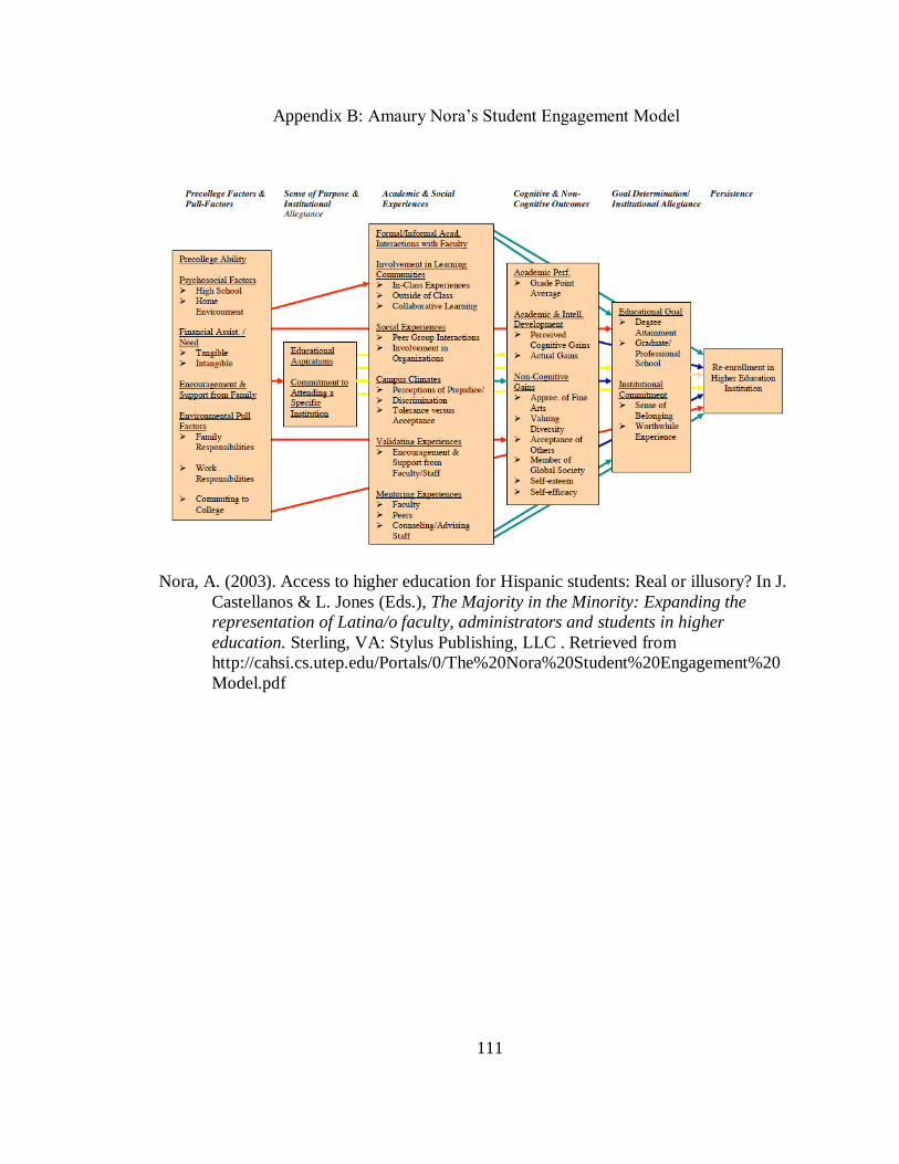
111
Appendix B: Amaury Nora’s Student Engagement Model
Nora, A. (2003). Access to higher education for Hispanic students: Real or illusory? In J.
Castellanos & L. Jones (Eds.), The Majority in the Minority: Expanding the
representation of Latina/o faculty, administrators and students in higher
education. Sterling, VA: Stylus Publishing, LLC . Retrieved from
http://cahsi.cs.utep.edu/Portals/0/The%20Nora%20Student%20Engagement%20
Model.pdf
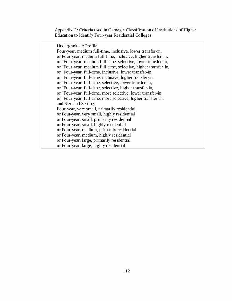
112
Appendix C: Criteria used in Carnegie Classification of Institutions of Higher
Education to Identify Four-year Residential Colleges
Undergraduate Profile:
Four-year, medium full-time, inclusive, lower transfer-in,
or Four-year, medium full-time, inclusive, higher transfer-in,
or "Four-year, medium full-time, selective, lower transfer-in,
or "Four-year, medium full-time, selective, higher transfer-in,
or "Four-year, full-time, inclusive, lower transfer-in,
or "Four-year, full-time, inclusive, higher transfer-in,
or "Four-year, full-time, selective, lower transfer-in,
or "Four-year, full-time, selective, higher transfer-in,
or "Four-year, full-time, more selective, lower transfer-in,
or "Four-year, full-time, more selective, higher transfer-in,
and Size and Setting:
Four-year, very small, primarily residential
or Four-year, very small, highly residential
or Four-year, small, primarily residential
or Four-year, small, highly residential
or Four-year, medium, primarily residential
or Four-year, medium, highly residential
or Four-year, large, primarily residential
or Four-year, large, highly residential
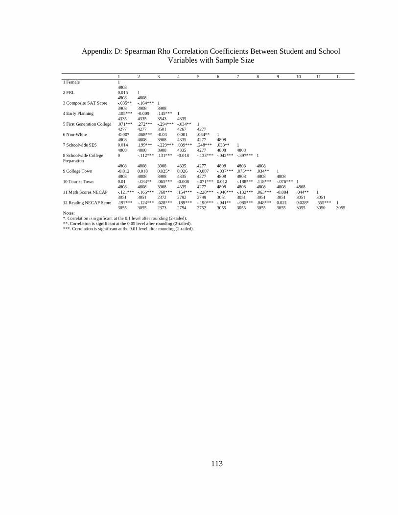
113
Appendix D: Spearman Rho Correlation Coefficients Between Student and School
Variables with Sample Size
1 2 3 4 5 6 7 8 9 10 11 12
1 Female 1
4808
2 FRL 0.015 1
4808 4808
3 Composite SAT Score -.035** -.164*** 1
3908 3908 3908
4 Early Planning .105*** -0.009 .145*** 1
4335 4335 3543 4335
5 First Generation College .071*** .272*** -.294*** -.034** 1
4277 4277 3501 4267 4277
6 Non-White -0.007 .068*** -0.03 0.001 .034** 1
4808 4808 3908 4335 4277 4808
7 Schoolwide SES 0.014 .199*** -.229*** .039*** .248*** .033** 1
4808 4808 3908 4335 4277 4808 4808
8 Schoolwide College
Preparation
0 -.112*** .131*** -0.018 -.133*** -.042*** -.397*** 1
4808 4808 3908 4335 4277 4808 4808 4808
9 College Town -0.012 0.018 0.025* 0.026 -0.007 -.037*** .075*** .034** 1
4808 4808 3908 4335 4277 4808 4808 4808 4808
10 Tourist Town 0.01 -.034** .065*** -0.008 -.071*** 0.012 -.188*** .118*** -.076*** 1
4808 4808 3908 4335 4277 4808 4808 4808 4808 4808
11 Math Scores NECAP -.121*** -.165*** .768*** .154*** -.228*** -.046*** -.132*** .063*** -0.004 .044** 1
3051 3051 2372 2792 2749 3051 3051 3051 3051 3051 3051
12 Reading NECAP Score .197*** -.124*** .628*** .189*** -.190*** -.041** -.085*** .048*** 0.021 0.028* .555*** 1
3055 3055 2373 2794 2752 3055 3055 3055 3055 3055 3050 3055
Notes:
*. Correlation is significant at the 0.1 level after rounding (2-tailed).
**. Correlation is significant at the 0.05 level after rounding (2-tailed).
***. Correlation is significant at the 0.01 level after rounding (2-tailed).

114
Appendix E: Variable Codes, Names, Definitions, and Literature Citation for Theoretical
Alignment to the Analysis
Variable Code Definition Citation School Factors (School) SIIPercNSLP2009
(Schoolwide SES) Percentage of high school (HS) students eligible for
the National School Lunch Program (NSLP) in
2009.
Niu & Tienda, 2013;
Johnson, 2008
SIIPercentSATTakers1012
(Schoolwide College
Preparation)
The mean percentage of students who took the SAT
from 2010, 2011, and 2012. Yan, 2002; Johnson
2008
Community Factors (Town) TIITouristTown
(Tourist Town) Binary code to indicate if the student lived in a
town with a high level of tourist activity. (Predictor)
Predictor
TIICollegeTown
(College Town) Binary code to indicate if the student lived in a rural
town with a college. (Predictor)
Predictor: Turley,
2009; Sage &
Sherman, 2014; Gibbs, 1998;
Johnson, 2008
Student Factors
Female
(Gender)
Binary code to indicate if the student was reported
as a female in the census.
Bean, 1980;
Howley, Johnson,
Passa, & Uekawa,
2014; Yan, 2002
FRL
(Low Family Income)
Binary code to indicate if a student was determined
eligible for free or reduced lunch or breakfast
through the National School Lunch Program.
Tinto, 1993; Bowen,
Chingos, &
McPherson, 2009
NotWhite (Non-White Race and
Ethnicity)
Binary code to indicate if the student was reported as being a race or ethnicity other than White.
Aud, Fox, & Kewal Ramani, 2010;
Bowen, Chingos &
McPherson, 2009;
Kao & Thompson,
2003
ZSATVERBMATHWRIT
(Composite SAT Score)
Standardized Composite SAT Verbal, Math and
Writing scores as most recently reported by the
College Board (measure of academic readiness).
College Board,
2016b; College
Board, 2016c; Hall,
et al., 2008; Stumpf
and Stanley, 2002
PARENTSNODEGREE
(First Generation College)
Binary variable that measures whether either parent
had attained an associate’s degree or more post-
secondary education.
Ishitani, 2006; Stage
& Hossler, 1988
EARLYTALK (Early Planning)
Binary variable that measures whether a student talked about their plans after high school in eighth
grade or earlier.
Hill & Wang, 2015; Stage & Hossler,
1988; Yan, 2002
Outcome Variable
CollegePersist
(College Persistence)
Binary code for students who were enrolled for the
fall and spring of their first two years attending a
four-year residential college.

115
Appendix F: SPSS Output of Coefficients for Collinearity Statistics
Model Summary
Model R R Square Adjusted R Square
Std. Error of the
Estimate
1 .675a .455 .452 7.206
a. Predictors: (Constant), MultiRaceEth, Female, Free or Reduced Lunch Eligibility, White, Post HS Talk Before Grade 9, Native Hawaiian or Pacific Islander, Zscore(SATVERBMATHWRIT), PARENTNODEGREE, American Indian, Asian, African American, Hispanic
Coefficientsa
Model
Unstandardized Coefficients
Standardized Coefficients
t Sig.
Collinearity Statistics
B Std. Error Beta Tolerance VIF
1 (Constant) 54.940 6.188 8.878 .000
Female 4.082 .316 .208 12.899 .000 .979 1.021
Free or Reduced Lunch Eligibility
.497 .408 .020 1.218 .223 .910 1.098
Zscore(SATVERBMATHWRIT) 6.191 .167 .631 37.157 .000 .885 1.130
PARENTNODEGREE -.367 .360 -.018 -1.018 .309 .857 1.167
Post HS Talk Before Grade 9 1.022 .329 .051 3.112 .002 .956 1.047
American Indian -4.980 6.627 -.038 -.751 .452 .099 10.093
African American -6.823 6.156 -.064 -1.108 .268 .077 13.024
Asian -2.836 6.436 -.027 -.441 .660 .070 14.238
Native Hawaiian or Pacific Islander
-6.062 6.119 -.019 -.991 .322 .694 1.441
Hispanic -2.852 6.352 -.029 -.449 .653 .059 16.918
White -3.874 6.189 -.048 -.626 .531 .043 23.253
MultiRaceEth 3.473 6.539 .047 .531 .595 .033 30.736
a. Dependent Variable: Reading NECAP Score Coefficientsa
Model
Unstandardized Coefficients
Standardized Coefficients
t Sig.
Collinearity Statistics
B Std. Error Beta Tolerance VIF
1 (Constant) 51.084 .281 181.572 .000
Female 4.085 .316 .208 12.919 .000 .980 1.020
Free or Reduced Lunch Eligibility
.457 .407 .019 1.124 .261 .914 1.094
Zscore(SATVERBMATHWRIT) 6.203 .166 .632 37.281 .000 .886 1.128
PARENTNODEGREE -.357 .360 -.017 -.992 .321 .859 1.164
Post HS Talk Before Grade 9 .988 .328 .049 3.015 .003 .961 1.041
NotWhite -.814 .890 -.015 -.915 .361 .994 1.006
a. Dependent Variable: Reading NECAP Score

116
Appendix G: SPSS Syntax for Constructing the College Persistence Variable
DO IF (((EnrollBegin1Quarter=3) OR (EnrollBegin1Quarter=4)) & (PSTerm1Year=2008)).
RECODE OPEID.1 (MISSING=0) (ELSE=Copy) INTO OPEIDFall2008.
END IF.
VARIABLE LABELS OPEIDFall2008 'OPEID for Fall Enrollment 2008'.
EXECUTE.
DO IF (((EnrollBegin2Quarter=1) & (PSTerm2Year=2009)) OR (((EnrollBegin2Quarter=4) &
(PSTerm2Year=2008)) & ((EnrollBegin3Quarter=1) & (PSTerm3Year=2009)) & (OPEID.2 = OPEID.3))).
RECODE OPEID.2 (MISSING=0) (ELSE=Copy) INTO OPEIDSpring2009.
VARIABLE LABELS OPEIDSpring2009 'OPEID for Enrollment Spring 2009'.
EXECUTE.
DO IF (((EnrollBegin3Quarter=3) & (PSTerm3Year=2009)) OR (((EnrollBegin4Quarter=3) &
(PSTerm4Year=2009)) OR ((EnrollBegin5Quarter=3)) & (PSTerm5Year=2009)) & ((OPEID.3 =
OPEID.4) OR (OPEID.3 = OPEID.5))).
RECODE OPEID.3 (MISSING=SYSMIS) (ELSE=Copy) INTO OPEIDFall2009.
END IF.
VARIABLE LABELS OPEIDFall2009 'OPEID for PS Enrollment Fall 2009'.
EXECUTE.
END IF.
DO IF (((EnrollBegin4Quarter=1) & (PSTerm4Year=2010)) OR ((EnrollBegin5Quarter=1) &
(PSTerm5Year=2010)) OR ((EnrollBegin6Quarter=1) & (PSTerm6Year=2010)) OR
(((EnrollBegin5Quarter=4) & (PSTerm5Year=2009)) & ((EnrollBegin6Quarter=1) &
(PSTerm6Year=2010)) OR ((EnrollBegin6Quarter=4) & (PSTerm6Year=2009)) & ((EnrollBegin7Quarter=1) & (PSTerm7Year=2010))) & ((OPEID.4 = OPEID.5) OR (OPEID.4 = OPEID.6)
OR (OPEID.4 = OPEID.7) OR (OPEID.4 = OPEID.8))).
RECODE OPEID.4 (MISSING=SYSMIS) (0 thru 9999999999999999=Copy) (ELSE=Copy) INTO
OPEIDSpring2010.
END IF.
VARIABLE LABELS OPEIDSpring2010 'OPEID for Enrollment Spring 2010'.
EXECUTE.
DO IF (OPEIDFall2008 = OPEIDSpring2010).
RECODE OPEIDFall2008 (MISSING=SYSMIS) (ELSE=Copy) INTO OPEIDFall08Spring2010.
END IF.
VARIABLE LABELS OPEIDFall08Spring2010 'Same OPEID for Fall 2008 and Spring 2010'.
EXECUTE.
COMPUTE TwoYears2008HSGrad=RANGE(OPEIDFall08Spring2010,1,9999999999999).
EXECUTE.
COMPUTE TwoYears2010HSGrad=RANGE(OPEIDFall10Spring2012,1,9999999999999).
EXECUTE.
COMPUTE TwoYears2012HSGrad=RANGE(OPEIDFall2012Spring2014,1,9999999999999).
EXECUTE.
COMPUTE PSPersistAllHSGrad=(TwoYears2008HSGrad=1) OR (TwoYears2010HSGrad=1) OR
(TwoYears2012HSGrad=1) = 1.
EXECUTE.
RECODE PSPersistAllHSGrad (1=1) (MISSING=0) (ELSE=Copy) INTO CollegePersist.
VARIABLE LABELS CollegePersist 'Added 0 to Missing Values on PSPersistAllHSGrad'.
EXECUTE.
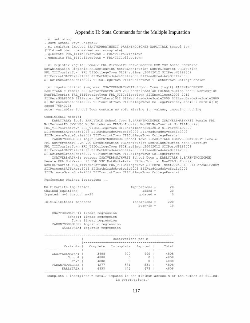
117
Appendix H: Stata Commands for the Multiple Imputation
. mi set mlong
. sort School Town UniqueID
. mi register imputed ZSATVERBMATHWRIT PARENTNODEGREE EARLYTALK School Town
(1314 m=0 obs. now marked as incomplete)
. generate FRL_TIITouristTown = FRL*TIITouristTown
. generate FRL_TIICollegeTown = FRL*TIICollegeTown
. mi register regular Female FRL VermontPS NotVermontPS UVM VSC Asian NotWhite
NotWhiteAsian Hispanic FRLNonTourist NonFRLNonTourist NonFRLTourist FRLTourist
FRL_TIITouristTown FRL_TIICollegeTown SIIEnrollment20052012 SIIPercNSLP2009
SIIPercentSATTakers1012 SIIMathGradeAveScale2009 SIIReadGradeAveScale2009
SIIScienceGradeScale2009 TIICollegeTown TIITouristTown TIIOtherTown CollegePersist
. mi impute chained (regress) ZSATVERBMATHWRIT School Town (logit) PARENTNODEGREE
EARLYTALK = Female FRL NotVermontPS UVM VSC NotWhiteAsian FRLNonTourist NonFRLNonTourist
NonFRLTourist FRL_TIITouristTown FRL_TIICollegeTown SIIEnrollment2005 2012
SIIPercNSLP2009 SIIPercentSATTakers1012 SIIMathGradeAveScale2009 SIIReadGradeAveScale2009
SIIScienceGradeScale2009 TIITouristTown TIICollegeTown CollegePersist, add(20) burnin(10)
rseed(7654321)
note: variables School Town contain no soft missing (.) values; imputing nothing
Conditional models:
EARLYTALK: logit EARLYTALK School Town i.PARENTNODEGREE ZSATVERBMATHWRIT Female FRL
NotVermontPS UVM VSC NotWhiteAsian FRLNonTourist NonFRLNonTourist NonFRLTourist
FRL_TIITouristTown FRL_TIICollegeTown SIIEnrollment20052012 SIIPercNSLP2009
SIIPercentSATTakers1012 SIIMathGradeAveScale2009 SIIReadGradeAveScale2009
SIIScienceGradeScale2009 TIITouristTown TIICollegeTown CollegePersist
PARENTNODEGREE: logit PARENTNODEGREE School Town i.EARLYTALK ZSATVERBMATHWRIT Female
FRL NotVermontPS UVM VSC NotWhiteAsian FRLNonTourist NonFRLNonTourist NonFRLTourist
FRL_TIITouristTown FRL_TIICollegeTown SIIEnrollment20052012 SIIPercNSLP2009
SIIPercentSATTakers1012 SIIMathGradeAveScale2009 SIIReadGradeAveScale2009
SIIScienceGradeScale2009 TIITouristTown TIICollegeTown CollegePersist
ZSATVERBMATH~T: regress ZSATVERBMATHWRIT School Town i.EARLYTALK i.PARENTNODEGREE
Female FRL NotVermontPS UVM VSC NotWhiteAsian FRLNonTourist NonFRLNonTourist
NonFRLTourist FRL_TIITouristTown FRL_TIICollegeTown SIIEnrollment20052012 SIIPercNSLP2009
SIIPercentSATTakers1012 SIIMathGradeAveScale2009 SIIReadGradeAveScale2009
SIIScienceGradeScale2009 TIITouristTown TIICollegeTown CollegePersist
Performing chained iterations ...
Multivariate imputation Imputations = 20
Chained equations added = 20
Imputed: m=1 through m=20 updated = 0
Initialization: monotone Iterations = 200
burn-in = 10
ZSATVERBMATH~T: linear regression
School: linear regression
Town: linear regression
PARENTNODEGREE: logistic regression
EARLYTALK: logistic regression
------------------------------------------------------------------
| Observations per m
|----------------------------------------------
Variable | Complete Incomplete Imputed | Total
-------------------+-----------------------------------+----------
ZSATVERBMATH~T | 3908 900 900 | 4808
School | 4808 0 0 | 4808
Town | 4808 0 0 | 4808
PARENTNODEGREE | 4277 531 531 | 4808
EARLYTALK | 4335 473 473 | 4808
------------------------------------------------------------------
(complete + incomplete = total; imputed is the minimum across m of the number of filled-
in observations.)
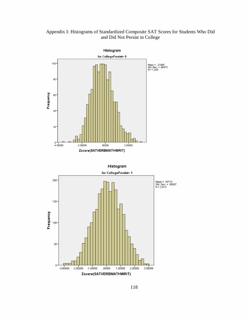
118
Appendix I: Histograms of Standardized Composite SAT Scores for Students Who Did
and Did Not Persist in College
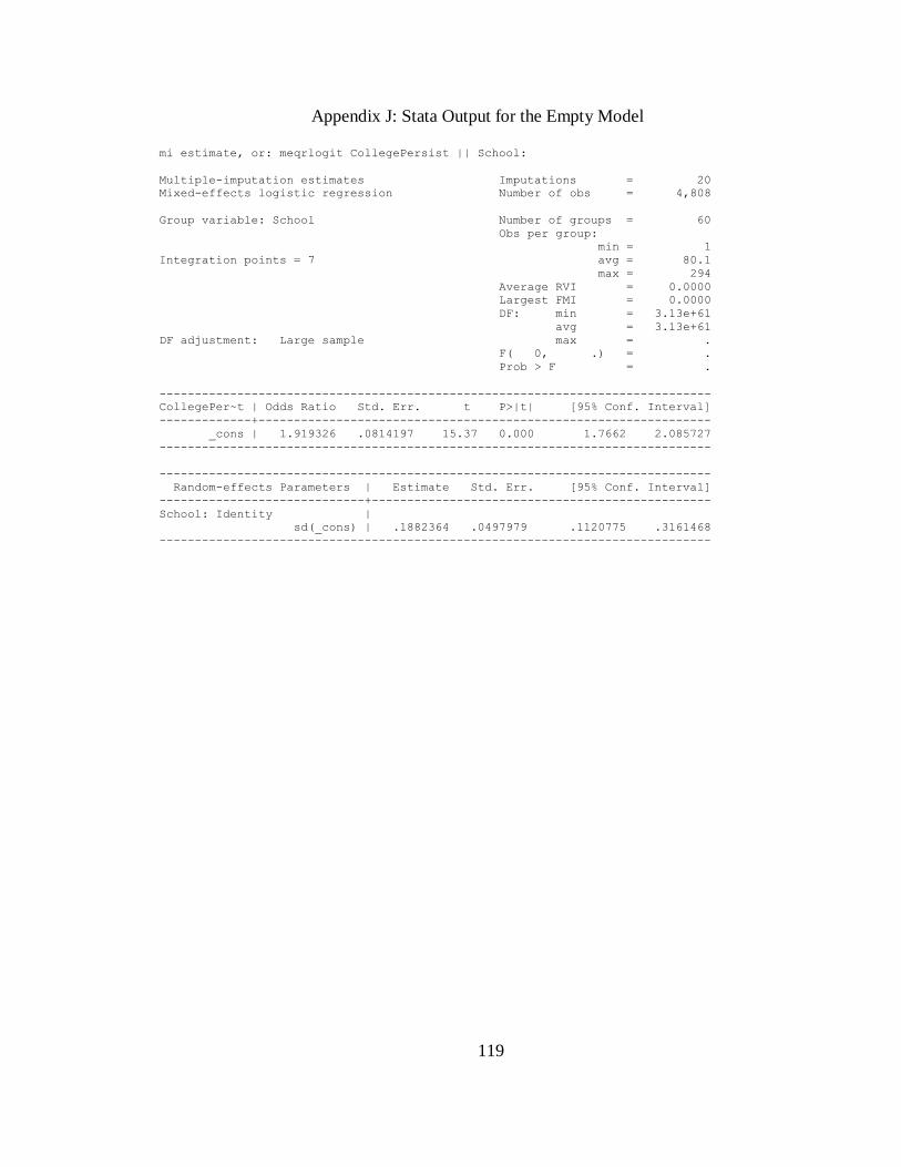
119
Appendix J: Stata Output for the Empty Model
mi estimate, or: meqrlogit CollegePersist || School:
Multiple-imputation estimates Imputations = 20
Mixed-effects logistic regression Number of obs = 4,808
Group variable: School Number of groups = 60
Obs per group:
min = 1
Integration points = 7 avg = 80.1
max = 294
Average RVI = 0.0000
Largest FMI = 0.0000
DF: min = 3.13e+61
avg = 3.13e+61
DF adjustment: Large sample max = .
F( 0, .) = .
Prob > F = .
------------------------------------------------------------------------------
CollegePer~t | Odds Ratio Std. Err. t P>|t| [95% Conf. Interval]
-------------+----------------------------------------------------------------
_cons | 1.919326 .0814197 15.37 0.000 1.7662 2.085727
------------------------------------------------------------------------------
------------------------------------------------------------------------------
Random-effects Parameters | Estimate Std. Err. [95% Conf. Interval]
-----------------------------+------------------------------------------------
School: Identity |
sd(_cons) | .1882364 .0497979 .1120775 .3161468
------------------------------------------------------------------------------
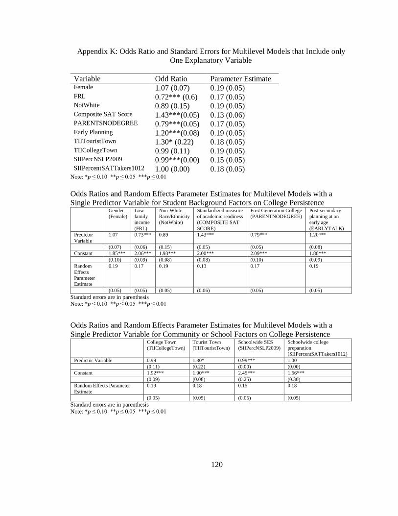
120
Appendix K: Odds Ratio and Standard Errors for Multilevel Models that Include only
One Explanatory Variable
Variable Odd Ratio Parameter Estimate Female 1.07 (0.07) 0.19 (0.05) FRL 0.72*** (0.6) 0.17 (0.05) NotWhite 0.89 (0.15) 0.19 (0.05) Composite SAT Score 1.43***(0.05) 0.13 (0.06) PARENTSNODEGREE 0.79***(0.05) 0.17 (0.05) Early Planning 1.20***(0.08) 0.19 (0.05) TIITouristTown 1.30* (0.22) 0.18 (0.05) TIICollegeTown 0.99 (0.11) 0.19 (0.05) SIIPercNSLP2009 0.99***(0.00) 0.15 (0.05) SIIPercentSATTakers1012 1.00 (0.00) 0.18 (0.05)
Note: *p ≤ 0.10 **p ≤ 0.05 ***p ≤ 0.01
Odds Ratios and Random Effects Parameter Estimates for Multilevel Models with a
Single Predictor Variable for Student Background Factors on College Persistence Gender
(Female)
Low
family
income
(FRL)
Non-White
Race/Ethnicity
(NotWhite)
Standardized measure
of academic readiness
(COMPOSITE SAT
SCORE)
First Generation College
(PARENTNODEGREE)
Post-secondary
planning at an
early age
(EARLYTALK)
Predictor
Variable
1.07 0.73*** 0.89 1.43*** 0.79*** 1.20***
(0.07) (0.06) (0.15) (0.05) (0.05) (0.08)
Constant 1.85*** 2.06*** 1.93*** 2.00*** 2.09*** 1.80***
(0.10) (0.09) (0.08) (0.08) (0.10) (0.09)
Random
Effects
Parameter
Estimate
0.19 0.17 0.19 0.13 0.17 0.19
(0.05) (0.05) (0.05) (0.06) (0.05) (0.05)
Standard errors are in parenthesis Note: *p ≤ 0.10 **p ≤ 0.05 ***p ≤ 0.01
Odds Ratios and Random Effects Parameter Estimates for Multilevel Models with a
Single Predictor Variable for Community or School Factors on College Persistence
College Town
(TIICollegeTown)
Tourist Town
(TIITouristTown)
Schoolwide SES
(SIIPercNSLP2009)
Schoolwide college
preparation
(SIIPercentSATTakers1012)
Predictor Variable 0.99 1.30* 0.99*** 1.00
(0.11) (0.22) (0.00) (0.00)
Constant 1.92*** 1.90*** 2.45*** 1.66***
(0.09) (0.08) (0.25) (0.30)
Random Effects Parameter
Estimate
0.19 0.18 0.15 0.18
(0.05) (0.05) (0.05) (0.05)
Standard errors are in parenthesis
Note: *p ≤ 0.10 **p ≤ 0.05 ***p ≤ 0.01

121
Appendix L: Stata Commands and Output from Multilevel Models
. mi estimate, or: meqrlogit CollegePersist || School:
Multiple-imputation estimates Imputations = 20
Mixed-effects logistic regression Number of obs = 4,808
Group variable: School Number of groups = 60
Obs per group:
min = 1
Integration points = 7 avg = 80.1
max = 294
Average RVI = 0.0000
Largest FMI = 0.0000
DF: min = 3.13e+61
avg = 3.13e+61
DF adjustment: Large sample max = .
F( 0, .) = .
Prob > F = .
------------------------------------------------------------------------------
CollegePer~t | Odds Ratio Std. Err. t P>|t| [95% Conf. Interval]
-------------+----------------------------------------------------------------
_cons | 1.919326 .0814197 15.37 0.000 1.7662 2.085727
------------------------------------------------------------------------------
------------------------------------------------------------------------------
Random-effects Parameters | Estimate Std. Err. [95% Conf. Interval]
-----------------------------+------------------------------------------------
School: Identity |
sd(_cons) | .1882364 .0497979 .1120775 .3161468
------------------------------------------------------------------------------
. mi estimate, or: meqrlogit CollegePersist Female || School:
Multiple-imputation estimates Imputations = 20
Mixed-effects logistic regression Number of obs = 4,808
Group variable: School Number of groups = 60
Obs per group:
min = 1
Integration points = 7 avg = 80.1
max = 294
Average RVI = 0.0000
Largest FMI = 0.0000
DF adjustment: Large sample DF: min = .
avg = .
max = .
Model F test: Equal FMI F( 1, .) = 1.22
Prob > F = 0.2693
------------------------------------------------------------------------------
CollegePer~t | Odds Ratio Std. Err. t P>|t| [95% Conf. Interval]
-------------+----------------------------------------------------------------
Female | 1.070287 .0658188 1.10 0.269 .9487558 1.207386
_cons | 1.849389 .1000657 11.36 0.000 1.663305 2.056291
------------------------------------------------------------------------------
------------------------------------------------------------------------------
Random-effects Parameters | Estimate Std. Err. [95% Conf. Interval]
-----------------------------+------------------------------------------------
School: Identity |
sd(_cons) | .189247 .0499688 .1127918 .3175267
------------------------------------------------------------------------------
. mi estimate, or: meqrlogit CollegePersist FRL || School:
Multiple-imputation estimates Imputations = 20
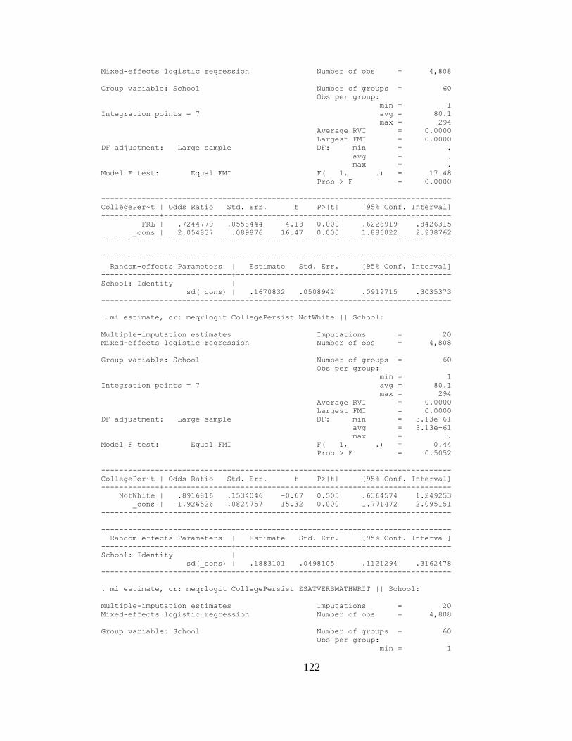
122
Mixed-effects logistic regression Number of obs = 4,808
Group variable: School Number of groups = 60
Obs per group:
min = 1
Integration points = 7 avg = 80.1
max = 294
Average RVI = 0.0000
Largest FMI = 0.0000
DF adjustment: Large sample DF: min = .
avg = .
max = .
Model F test: Equal FMI F( 1, .) = 17.48
Prob > F = 0.0000
------------------------------------------------------------------------------
CollegePer~t | Odds Ratio Std. Err. t P>|t| [95% Conf. Interval]
-------------+----------------------------------------------------------------
FRL | .7244779 .0558444 -4.18 0.000 .6228919 .8426315
_cons | 2.054837 .089876 16.47 0.000 1.886022 2.238762
------------------------------------------------------------------------------
------------------------------------------------------------------------------
Random-effects Parameters | Estimate Std. Err. [95% Conf. Interval]
-----------------------------+------------------------------------------------
School: Identity |
sd(_cons) | .1670832 .0508942 .0919715 .3035373
------------------------------------------------------------------------------
. mi estimate, or: meqrlogit CollegePersist NotWhite || School:
Multiple-imputation estimates Imputations = 20
Mixed-effects logistic regression Number of obs = 4,808
Group variable: School Number of groups = 60
Obs per group:
min = 1
Integration points = 7 avg = 80.1
max = 294
Average RVI = 0.0000
Largest FMI = 0.0000
DF adjustment: Large sample DF: min = 3.13e+61
avg = 3.13e+61
max = .
Model F test: Equal FMI F( 1, .) = 0.44
Prob > F = 0.5052
------------------------------------------------------------------------------
CollegePer~t | Odds Ratio Std. Err. t P>|t| [95% Conf. Interval]
-------------+----------------------------------------------------------------
NotWhite | .8916816 .1534046 -0.67 0.505 .6364574 1.249253
_cons | 1.926526 .0824757 15.32 0.000 1.771472 2.095151
------------------------------------------------------------------------------
------------------------------------------------------------------------------
Random-effects Parameters | Estimate Std. Err. [95% Conf. Interval]
-----------------------------+------------------------------------------------
School: Identity |
sd(_cons) | .1883101 .0498105 .1121294 .3162478
------------------------------------------------------------------------------
. mi estimate, or: meqrlogit CollegePersist ZSATVERBMATHWRIT || School:
Multiple-imputation estimates Imputations = 20
Mixed-effects logistic regression Number of obs = 4,808
Group variable: School Number of groups = 60
Obs per group:
min = 1
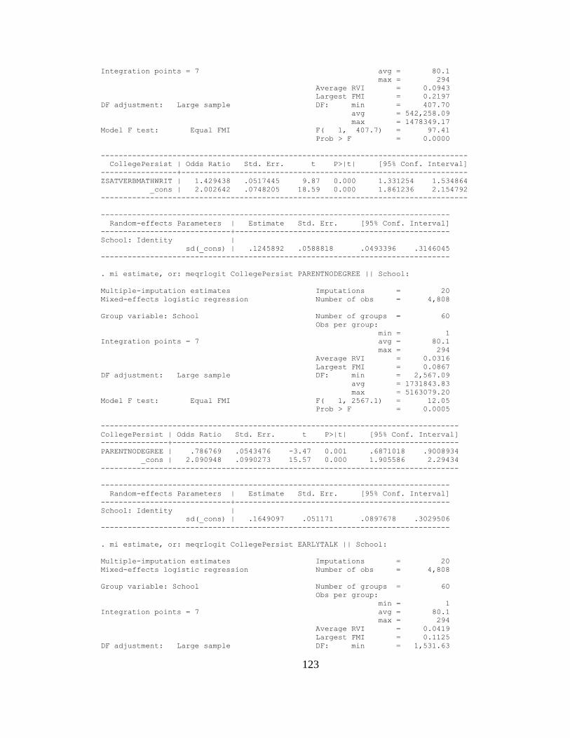
123
Integration points = 7 avg = 80.1
max = 294
Average RVI = 0.0943
Largest FMI = 0.2197
DF adjustment: Large sample DF: min = 407.70
avg = 542,258.09
max = 1478349.17
Model F test: Equal FMI F( 1, 407.7) = 97.41
Prob > F = 0.0000
----------------------------------------------------------------------------------
CollegePersist | Odds Ratio Std. Err. t P>|t| [95% Conf. Interval]
-----------------+----------------------------------------------------------------
ZSATVERBMATHWRIT | 1.429438 .0517445 9.87 0.000 1.331254 1.534864
_cons | 2.002642 .0748205 18.59 0.000 1.861236 2.154792
----------------------------------------------------------------------------------
------------------------------------------------------------------------------
Random-effects Parameters | Estimate Std. Err. [95% Conf. Interval]
-----------------------------+------------------------------------------------
School: Identity |
sd(_cons) | .1245892 .0588818 .0493396 .3146045
------------------------------------------------------------------------------
. mi estimate, or: meqrlogit CollegePersist PARENTNODEGREE || School:
Multiple-imputation estimates Imputations = 20
Mixed-effects logistic regression Number of obs = 4,808
Group variable: School Number of groups = 60
Obs per group:
min = 1
Integration points = 7 avg = 80.1
max = 294
Average RVI = 0.0316
Largest FMI = 0.0867
DF adjustment: Large sample DF: min = 2,567.09
avg = 1731843.83
max = 5163079.20
Model F test: Equal FMI F( 1, 2567.1) = 12.05
Prob > F = 0.0005
--------------------------------------------------------------------------------
CollegePersist | Odds Ratio Std. Err. t P>|t| [95% Conf. Interval]
---------------+----------------------------------------------------------------
PARENTNODEGREE | .786769 .0543476 -3.47 0.001 .6871018 .9008934
_cons | 2.090948 .0990273 15.57 0.000 1.905586 2.29434
--------------------------------------------------------------------------------
------------------------------------------------------------------------------
Random-effects Parameters | Estimate Std. Err. [95% Conf. Interval]
-----------------------------+------------------------------------------------
School: Identity |
sd(_cons) | .1649097 .051171 .0897678 .3029506
------------------------------------------------------------------------------
. mi estimate, or: meqrlogit CollegePersist EARLYTALK || School:
Multiple-imputation estimates Imputations = 20
Mixed-effects logistic regression Number of obs = 4,808
Group variable: School Number of groups = 60
Obs per group:
min = 1
Integration points = 7 avg = 80.1
max = 294
Average RVI = 0.0419
Largest FMI = 0.1125
DF adjustment: Large sample DF: min = 1,531.63

124
avg = 3.30e+07
max = 9.91e+07
Model F test: Equal FMI F( 1, 1531.6) = 7.01
Prob > F = 0.0082
------------------------------------------------------------------------------
CollegePer~t | Odds Ratio Std. Err. t P>|t| [95% Conf. Interval]
-------------+----------------------------------------------------------------
EARLYTALK | 1.197928 .0816977 2.65 0.008 1.047933 1.369392
_cons | 1.796671 .0885468 11.89 0.000 1.631234 1.978887
------------------------------------------------------------------------------
------------------------------------------------------------------------------
Random-effects Parameters | Estimate Std. Err. [95% Conf. Interval]
-----------------------------+------------------------------------------------
School: Identity |
sd(_cons) | .1914287 .0497718 .1149988 .3186551
------------------------------------------------------------------------------
. mi estimate, or: meqrlogit CollegePersist TIICollegeTown || School:
Multiple-imputation estimates Imputations = 20
Mixed-effects logistic regression Number of obs = 4,808
Group variable: School Number of groups = 60
Obs per group:
min = 1
Integration points = 7 avg = 80.1
max = 294
Average RVI = 0.0000
Largest FMI = 0.0000
DF adjustment: Large sample DF: min = 3.30e+61
avg = 3.30e+61
max = .
Model F test: Equal FMI F( 1, .) = 0.00
Prob > F = 0.9607
--------------------------------------------------------------------------------
CollegePersist | Odds Ratio Std. Err. t P>|t| [95% Conf. Interval]
---------------+----------------------------------------------------------------
TIICollegeTown | .9943571 .1142914 -0.05 0.961 .7937894 1.245603
_cons | 1.920512 .0848958 14.76 0.000 1.761123 2.094325
--------------------------------------------------------------------------------
------------------------------------------------------------------------------
Random-effects Parameters | Estimate Std. Err. [95% Conf. Interval]
-----------------------------+------------------------------------------------
School: Identity |
sd(_cons) | .1878738 .0503522 .1111054 .3176853
------------------------------------------------------------------------------
. mi estimate, or: meqrlogit CollegePersist TIITouristTown || School:
Multiple-imputation estimates Imputations = 20
Mixed-effects logistic regression Number of obs = 4,808
Group variable: School Number of groups = 60
Obs per group:
min = 1
Integration points = 7 avg = 80.1
max = 294
Average RVI = 0.0000
Largest FMI = 0.0000
DF adjustment: Large sample DF: min = .
avg = .
max = .
Model F test: Equal FMI F( 1, .) = 2.49
Prob > F = 0.1142
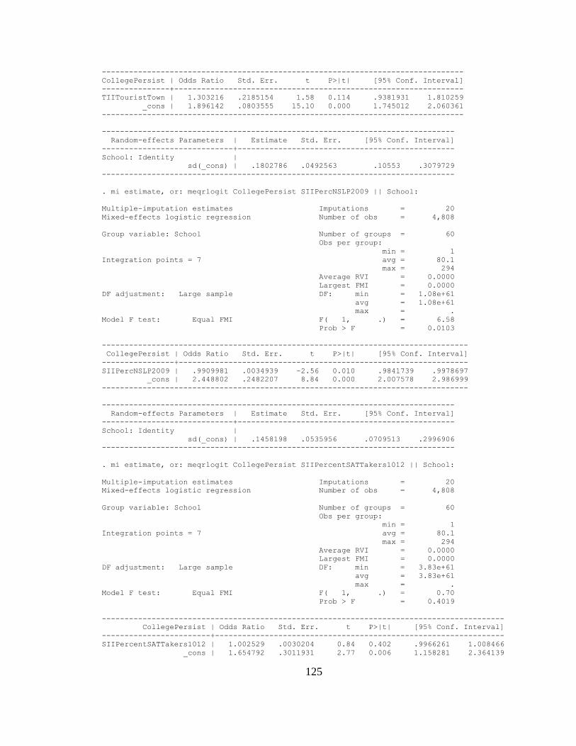
125
--------------------------------------------------------------------------------
CollegePersist | Odds Ratio Std. Err. t P>|t| [95% Conf. Interval]
---------------+----------------------------------------------------------------
TIITouristTown | 1.303216 .2185154 1.58 0.114 .9381931 1.810259
_cons | 1.896142 .0803555 15.10 0.000 1.745012 2.060361
--------------------------------------------------------------------------------
------------------------------------------------------------------------------
Random-effects Parameters | Estimate Std. Err. [95% Conf. Interval]
-----------------------------+------------------------------------------------
School: Identity |
sd(_cons) | .1802786 .0492563 .10553 .3079729
------------------------------------------------------------------------------
. mi estimate, or: meqrlogit CollegePersist SIIPercNSLP2009 || School:
Multiple-imputation estimates Imputations = 20
Mixed-effects logistic regression Number of obs = 4,808
Group variable: School Number of groups = 60
Obs per group:
min = 1
Integration points = 7 avg = 80.1
max = 294
Average RVI = 0.0000
Largest FMI = 0.0000
DF adjustment: Large sample DF: min = 1.08e+61
avg = 1.08e+61
max = .
Model F test: Equal FMI F( 1, .) = 6.58
Prob > F = 0.0103
---------------------------------------------------------------------------------
CollegePersist | Odds Ratio Std. Err. t P>|t| [95% Conf. Interval]
----------------+----------------------------------------------------------------
SIIPercNSLP2009 | .9909981 .0034939 -2.56 0.010 .9841739 .9978697
_cons | 2.448802 .2482207 8.84 0.000 2.007578 2.986999
---------------------------------------------------------------------------------
------------------------------------------------------------------------------
Random-effects Parameters | Estimate Std. Err. [95% Conf. Interval]
-----------------------------+------------------------------------------------
School: Identity |
sd(_cons) | .1458198 .0535956 .0709513 .2996906
------------------------------------------------------------------------------
. mi estimate, or: meqrlogit CollegePersist SIIPercentSATTakers1012 || School:
Multiple-imputation estimates Imputations = 20
Mixed-effects logistic regression Number of obs = 4,808
Group variable: School Number of groups = 60
Obs per group:
min = 1
Integration points = 7 avg = 80.1
max = 294
Average RVI = 0.0000
Largest FMI = 0.0000
DF adjustment: Large sample DF: min = 3.83e+61
avg = 3.83e+61
max = .
Model F test: Equal FMI F( 1, .) = 0.70
Prob > F = 0.4019
-----------------------------------------------------------------------------------------
CollegePersist | Odds Ratio Std. Err. t P>|t| [95% Conf. Interval]
------------------------+----------------------------------------------------------------
SIIPercentSATTakers1012 | 1.002529 .0030204 0.84 0.402 .9966261 1.008466
_cons | 1.654792 .3011931 2.77 0.006 1.158281 2.364139
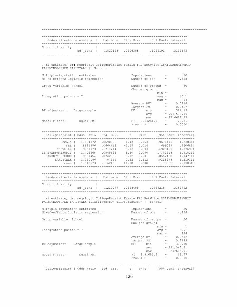
126
-----------------------------------------------------------------------------------------
------------------------------------------------------------------------------
Random-effects Parameters | Estimate Std. Err. [95% Conf. Interval]
-----------------------------+------------------------------------------------
School: Identity |
sd(_cons) | .1820153 .0506308 .1055191 .3139675
------------------------------------------------------------------------------
. mi estimate, or: meqrlogit CollegePersist Female FRL NotWhite ZSATVERBMATHWRIT
PARENTNODEGREE EARLYTALK || School:
Multiple-imputation estimates Imputations = 20
Mixed-effects logistic regression Number of obs = 4,808
Group variable: School Number of groups = 60
Obs per group:
min = 1
Integration points = 7 avg = 80.1
max = 294
Average RVI = 0.0718
Largest FMI = 0.2467
DF adjustment: Large sample DF: min = 324.13
avg = 704,539.79
max = 2716629.23
Model F test: Equal FMI F( 6,14261.0) = 20.36
Prob > F = 0.0000
----------------------------------------------------------------------------------
CollegePersist | Odds Ratio Std. Err. t P>|t| [95% Conf. Interval]
-----------------+----------------------------------------------------------------
Female | 1.094372 .0690088 1.43 0.153 .9671411 1.238341
FRL | .8194856 .0664668 -2.45 0.014 .699039 .9606854
NotWhite | .9767973 .1711244 -0.13 0.893 .6929199 1.376974
ZSATVERBMATHWRIT | 1.406668 .0545633 8.80 0.000 1.303318 1.518213
PARENTNODEGREE | .9907454 .0742839 -0.12 0.901 .8552468 1.147711
EARLYTALK | 1.060186 .07555 0.82 0.412 .9218278 1.219311
_cons | 1.948673 .1162409 11.18 0.000 1.73365 2.190365
----------------------------------------------------------------------------------
------------------------------------------------------------------------------
Random-effects Parameters | Estimate Std. Err. [95% Conf. Interval]
-----------------------------+------------------------------------------------
School: Identity |
sd(_cons) | .1210277 .0598405 .0459218 .3189702
------------------------------------------------------------------------------
. mi estimate, or: meqrlogit CollegePersist Female FRL NotWhite ZSATVERBMATHWRIT
PARENTNODEGREE EARLYTALK TIICollegeTown TIITouristTown || School:
Multiple-imputation estimates Imputations = 20
Mixed-effects logistic regression Number of obs = 4,808
Group variable: School Number of groups = 60
Obs per group:
min = 1
Integration points = 7 avg = 80.1
max = 294
Average RVI = 0.0587
Largest FMI = 0.2483
DF adjustment: Large sample DF: min = 320.10
avg = 621,065.91
max = 2347605.96
Model F test: Equal FMI F( 8,31653.5) = 15.77
Prob > F = 0.0000
----------------------------------------------------------------------------------
CollegePersist | Odds Ratio Std. Err. t P>|t| [95% Conf. Interval]

127
-----------------+----------------------------------------------------------------
Female | 1.092656 .0689152 1.40 0.160 .9655989 1.236431
FRL | .8206918 .0665518 -2.44 0.015 .7000895 .9620699
NotWhite | .9718983 .1703034 -0.16 0.871 .6893928 1.370171
ZSATVERBMATHWRIT | 1.40553 .0545924 8.76 0.000 1.302126 1.517145
PARENTNODEGREE | .9940021 .0746169 -0.08 0.936 .8579058 1.151688
EARLYTALK | 1.061501 .0756511 0.84 0.403 .9229579 1.22084
TIICollegeTown | .9500144 .1058972 -0.46 0.646 .7635673 1.181988
TIITouristTown | 1.178711 .188451 1.03 0.304 .8616242 1.612488
_cons | 1.941827 .1188663 10.84 0.000 1.722278 2.189362
----------------------------------------------------------------------------------
------------------------------------------------------------------------------
Random-effects Parameters | Estimate Std. Err. [95% Conf. Interval]
-----------------------------+------------------------------------------------
School: Identity |
sd(_cons) | .1144902 .0625038 .0392708 .3337847
------------------------------------------------------------------------------
. mi estimate, or: meqrlogit CollegePersist Female FRL NotWhite ZSATVERBMATHWRIT
PARENTNODEGREE EARLYTALK TIICollegeTown TIITouristTown SIIPercNSLP2009
SIIPercentSATTakers1012 || School:
Multiple-imputation estimates Imputations = 20
Mixed-effects logistic regression Number of obs = 4,808
Group variable: School Number of groups = 60
Obs per group:
min = 1
Integration points = 7 avg = 80.1
max = 294
Average RVI = 0.0500
Largest FMI = 0.2516
DF adjustment: Large sample DF: min = 312.00
avg = 786,931.30
max = 2161128.88
Model F test: Equal FMI F( 10,58314.1) = 12.78
Prob > F = 0.0000
-----------------------------------------------------------------------------------------
CollegePersist | Odds Ratio Std. Err. t P>|t| [95% Conf. Interval]
------------------------+----------------------------------------------------------------
Female | 1.09271 .0689245 1.41 0.160 .9656371 1.236506
FRL | .8213649 .0670056 -2.41 0.016 .6999969 .9637762
NotWhite | .9716382 .1703309 -0.16 0.870 .6891067 1.370007
ZSATVERBMATHWRIT | 1.405178 .055226 8.66 0.000 1.300611 1.518152
PARENTNODEGREE | .9947177 .0752938 -0.07 0.944 .8574725 1.15393
EARLYTALK | 1.061662 .0758801 0.84 0.403 .9227239 1.22152
TIICollegeTown | .9512646 .1062629 -0.45 0.655 .7642158 1.184095
TIITouristTown | 1.177288 .190342 1.01 0.313 .8575548 1.616232
SIIPercNSLP2009 | .9995445 .0036274 -0.13 0.900 .9924602 1.006679
SIIPercentSATTakers1012 | .99959 .0027961 -0.15 0.883 .9941247 1.005085
_cons | 2.012072 .4338164 3.24 0.001 1.318617 3.070214
-----------------------------------------------------------------------------------------
------------------------------------------------------------------------------
Random-effects Parameters | Estimate Std. Err. [95% Conf. Interval]
-----------------------------+------------------------------------------------
School: Identity |
sd(_cons) | .1145281 .0625431 .0392714 .3340013
------------------------------------------------------------------------------
. mi estimate, or: meqrlogit CollegePersist Female NotWhite ZSATVERBMATHWRIT
PARENTNODEGREE EARLYTALK NonFRLNonTourist No
> nFRLTourist TIICollegeTown SIIPercNSLP2009 SIIPercentSATTakers1012 || School:
Multiple-imputation estimates Imputations = 20
Mixed-effects logistic regression Number of obs = 4,808
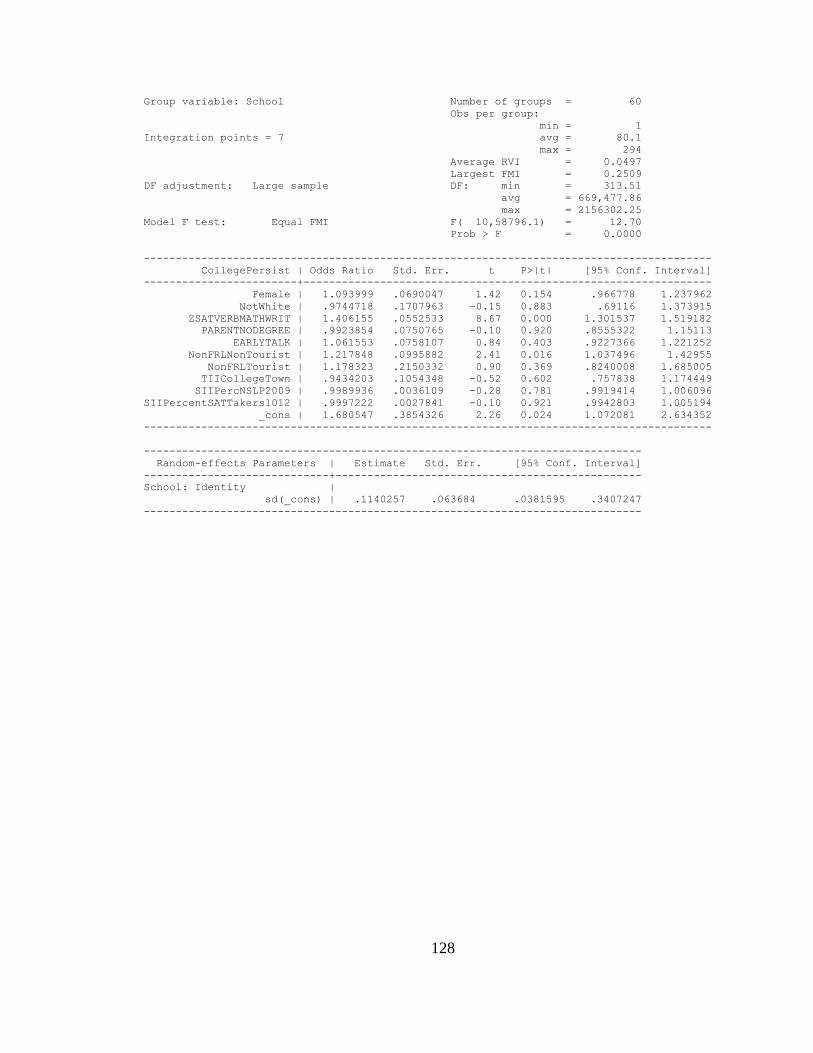
128
Group variable: School Number of groups = 60
Obs per group:
min = 1
Integration points = 7 avg = 80.1
max = 294
Average RVI = 0.0497
Largest FMI = 0.2509
DF adjustment: Large sample DF: min = 313.51
avg = 669,477.86
max = 2156302.25
Model F test: Equal FMI F( 10,58796.1) = 12.70
Prob > F = 0.0000
-----------------------------------------------------------------------------------------
CollegePersist | Odds Ratio Std. Err. t P>|t| [95% Conf. Interval]
------------------------+----------------------------------------------------------------
Female | 1.093999 .0690047 1.42 0.154 .966778 1.237962
NotWhite | .9744718 .1707963 -0.15 0.883 .69116 1.373915
ZSATVERBMATHWRIT | 1.406155 .0552533 8.67 0.000 1.301537 1.519182
PARENTNODEGREE | .9923854 .0750765 -0.10 0.920 .8555322 1.15113
EARLYTALK | 1.061553 .0758107 0.84 0.403 .9227366 1.221252
NonFRLNonTourist | 1.217848 .0995882 2.41 0.016 1.037496 1.42955
NonFRLTourist | 1.178323 .2150332 0.90 0.369 .8240008 1.685005
TIICollegeTown | .9434203 .1054348 -0.52 0.602 .757838 1.174449
SIIPercNSLP2009 | .9989936 .0036109 -0.28 0.781 .9919414 1.006096
SIIPercentSATTakers1012 | .9997222 .0027841 -0.10 0.921 .9942803 1.005194
_cons | 1.680547 .3854326 2.26 0.024 1.072081 2.634352
-----------------------------------------------------------------------------------------
------------------------------------------------------------------------------
Random-effects Parameters | Estimate Std. Err. [95% Conf. Interval]
-----------------------------+------------------------------------------------
School: Identity |
sd(_cons) | .1140257 .063684 .0381595 .3407247
------------------------------------------------------------------------------