Embed Size (px)
Citation preview
1
An examination of Echoic Flow based autonomous guidance
using the Lego Mindstorms NXT robot
Undergraduate Research Distinction Thesis
Presented in Partial Fulfillment of the Requirements for the Degree Bachelor of Science
with Research Distinction at The Ohio State University
By
Yuyao Chen
Department of Electrical and Computer Engineering
The Ohio State University
Research Advisor:
Prof. Chris Baker
2
Abstract
It is well known that some animals, such as bats, can find their routes home autonomously and
are able to avoid crashing into each other while traveling in a group. They do this using
echolocation that enables them to function at dusk and in the dark. My research project is to
investigate how these complicated behaviors can be replicated using robot vehicles that have
echolocation sensors. Echoic flow fields are computed and simple rules to govern subsequent
behavior are implemented. Echoic flow is defined to be the ratio of a sensed parameter such as
range or intensity to a change in that parameter per unit time. The ratio of these two quantities
gives the time over which two bodies will come into contact (collide). This “time to collision”
can be used to provide feedback to the robot to either avoid collisions or to control the form of a
collision. Previous theoretical research has shown that echoic flow can be used to control the
behaviors of objects in relative motion. Experimental work has shown that the Lego NXT robot
and its ultrasonic echolocation sensors can enable obstacle avoidance. My project develops
extends this earlier experimental research to determine if echoic flow can be used to control two
robots so that one leads and has to avoid obstacles as it autonomously navigates a course while
the other follows the first robot maintaining a constant time to collision. In order to accomplish
this experiment, two robots are needed. The leading robot can be controlled by a remote control
with a vertical flat board, and the following robot is Lego NXT robot which can be programmed
by Matlab and it also has two ultrasonic sensors connected by wires. The function of ultrasonic
sensors is to test the range from current position to the detected object which is a solid board.
This project helps us to understand bat’s echolocation behavior by applying echoic flow theorem
to Lego NXT robot with ultrasonic sensors.

3
Acknowledgement
I would like to thanks Prof. Baker and Dr. Smith for their help in guiding me to a good direction
of my research project and also in teaching me the knowledge which I am not very familiar with.
Not only their professional and resourceful knowledge did help me to do better in my project, but
their patience in teaching and guiding me is also a big encouragement for performing better in
my undergraduate research project.
It is Prof. Baker who brought me to the research world and I really want to thank him for giving
me such an opportunity to apply the knowledge I learned from class to practice. He gave me a
general idea about the goal of the project at first, and then he will help me cut a general idea to
small pieces which are the short-term goals to be finished.
Dr. Smith is my research co-advisor. Prof. Baker gives me a general idea to work on and Dr.
Smith sets up a meeting with me every week to talk about the steps of the project specifically.
After one-week’s work, I report to Dr. Smith about the result of what I am working on, like both
progress I’ve made and failures I’ve met. When I firstly came to the cognitive science lab and
knew little about it, then it was Dr. Smith’s patience on me and clear explanations that make me
quickly get involved in this project. I would like to say, Dr. Smith made a lot of contribution in
guiding undergraduate researchers, because he knows clearly the difference between an
undergraduate and graduate researcher, so he can guide undergraduate researchers in a way in
which undergraduates can accept and grasp knowledge well.
I also would like to thanks PhD students Saif Alsaif and Landon Garry for their valuable advice
and help when I got stuck and confused about what to do for the next step. Sometimes, it was
just one piece of their suggestion which can generate the possible solution.
In a word, my undergraduate research project cannot be accomplished without their continuous
help and patient guidance. Finally, I want to thanks the College of Engineering and
Undergraduate Research Office for awarding me the scholarship of excellent undergraduate
research proposal.
4
Contents
Abstract ......................................................................................................................................................... 2
Acknowledgement ........................................................................................................................................ 3
Chapter 1: Introduction ................................................................................................................................ 6
1.1 Introduction .................................................................................................................................. 6
Chapter 2: Background Theories................................................................................................................... 7
2.2 Differences between sound and radio wave Echolocation working principles .................................. 9
2.3 Introduction to Ultrasound wave and Ultrasonic ............................................................................. 10
2.4 Echoic Flow Theorem ........................................................................................................................ 11
2.4.1 Application of Echoic Flow Theorem in experiments .................................................................... 11
2.5 Robotics Control ................................................................................................................................ 13
2.6 Linear Regression .............................................................................................................................. 14
2.7 Background research ........................................................................................................................ 15
Chapter 3: Introduction to equipment and setup ...................................................................................... 16
3.1 Hardwire: Lego Mindstorms NXT 2.0 ................................................................................................ 16
3.1.1 Ultrasonic Sensor ........................................................................................................................... 16
3.1.2 Interactive Servo Motor ................................................................................................................. 17
3.1.3 USB Port and a 16 feet USB-A Male to USB-B Male cable ............................................................. 18
3.2 Software Used: MATLAB 2012b (Windows 32 bit) ........................................................................... 18
3.2.1 Lego Mindstorms NXT 2.0 Phanton Driver .................................................................................... 18
Chapter 4: Calibration of Lego Sensors ....................................................................................................... 20
4.1 The need for calibration in experiments ........................................................................................... 20
4.2 Ultrasonic sensor range measurement ............................................................................................. 20
4.2.1 Introduction to Buffer and Buffersize ............................................................................................ 21
4.2.2 Experiment setup for testing the most appropriate value of buffersize ....................................... 22
4.2.3 Methods used to decide the result of buffersize ........................................................................... 22
a. Use range measured by ultrasonic sensor to compare difference values of buffer-size ............... 22
b. Use echoic flow calculated by equation (1) to compare difference values of buffer-size ............. 24
4.2.4 Conclusion of Buffer-size testing ................................................................................................... 25
4.3 Calibration when two sensors work together .................................................................................. 26
4.4 Different angles of robot setting....................................................................................................... 28
5
4.5 Testing the alternative way to compute echoic flow, τ(r) = 𝒓𝒗 ∗ 𝐜𝐨𝐬(ө) , when ultrasonic sensors
are set in different angles ....................................................................................................................... 29
Chapter 5: Experiment Work ...................................................................................................................... 31
5.1 Experiment 1: Lego robot move straight forward and keep a fixed distance from an object while
following an object ..................................................................................................................................... 31
5.1.1 Introduction of experiment1 ......................................................................................................... 31
5.1.2 Experiment Setup of experiment 1 ................................................................................................ 32
5.1.3 Algorithm of Experiment 1 ............................................................................................................. 33
5.1.4 Analysis of variables used in experiment 1 .................................................................................... 34
5.1.5 Future progress of experiment 1 ................................................................................................... 36
5.1.6 Conclusion of Experiment 1 ........................................................................................................... 36
5.2 Experiment 2: A Lego robot moving forward with two ultrasonic sensors following an object’s path 36
5.2.1 Introduction of Experiment 2 ..................................................................................................... 36
5.2.2 Setup of Experiment 2 ................................................................................................................... 37
5.2.3 Algorithm of Experiment 2 ............................................................................................................. 38
5.2.4 Analysis of variable used in Experiment 2 ..................................................................................... 39
5.3 Experiment 3: A Lego robot exactly is following the path of the other moving object ........................ 41
5.3.1 Introduction to experiment 3 ........................................................................................................ 41
5.3.3 Analysis of variables used in Experiment 3 .................................................................................... 44
5.3.4 Constraints in Experiment 3 ........................................................................................................... 44
5.3.5 Future progress of experiment 3 ................................................................................................... 45
5.3.6 Conclusion of experiment 3 ........................................................................................................... 45
Chapter 6: Conclusion ............................................................................................................................. 46
6.1 Overall Conclusion ............................................................................................................................ 46
6.2 Future application of the project ...................................................................................................... 46
Appendix I: Project Schedule .................................................................................................................. 48
Appendix II: Experiment 1 MATLAB code ............................................................................................... 49
Appendix III: Experiment 3 MATLAB code .............................................................................................. 51
Reference Page: ...................................................................................................................................... 55
6
Chapter 1: Introduction
1.1 Introduction
In real life, some mammals, like bats and whales, can find their routes to home autonomously or
follow their groups by echo locating. While echo locating, Bats send out a beam of sound wave
and then receive the echo reflected by the target. Through this process, bats can detect targets
and precisely know its location. They use this information to plan their routes.
This research project investigates how these complicated behaviors can be applied to a Lego
NXT robot. The concept of echoic flow, given the symbol τ, is defined to be the ratio of a sensor
measurable parameter to a change in that parameter, which is also the time to collision, τ(r) =r/�̇�,
where r is the range to a detected object and �̇� is the change in range of the object between the
current and previous measurement. The main experiment reported on is using echoic flow to
design a program which involves a Lego robot and a moving object. The robot can exactly
follow the moving object. The test environment for the Lego robot is a wooden square corridor
in ESL cognitive lab. The Lego NXT robot can be controlled by MATLAB because it has an
embedded programmable intelligent brick in which is a microcontroller. The robot has two
ultrasonic sensors which can measure the range from the robot to the detected object. The
anticipated result is that the Lego robot can exactly copy the path of the leading object while
keeping a fixed distance from it at the same time. Thus, we can see that the Lego robot
demonstrated the bats’ feature of autonomous navigation by applying echoic flow to the robot.
Before doing the experiment, calibration of the Lego equipment was undertaken to test the
accuracy of the experiment facilities. Another goal of calibration work is to determine the most
appropriate value of variables applied in MATLAB codes for controlling the robot. Since both
the external and internal factors will make a big difference to the result of the experiments, so
calibration work is indispensable for my research project. External factors include environment
noise and error in facilities, and internal factors consist of logic of programming and variables
chosen to control the robot.
7
1.2 Overview of the Thesis Organization
The report will cover background theorems applied in the project, introduction to the
experimental setup, calibration work involved in and the final experiment tests.
Chapter 2 is an introduction to the background theories which are applied in the research
project and the background research that has already been finished
Chapter 3 covered the experimental setup and an introduction to both software and
hardware used in the experiments
Chapter 4 focused on the calibration work which includes the test for the accuracy of
hardware and an examination to the variables used in programming
Chapter 5 emphasized on the three experiments accomplished and a detailed analysis of
the three experiments
Chapter 6 summarized the whole project and introduced the future work
Chapter 2: Background Theories
In this chapter, theorems and methods which are involved in the experiments and calibration
work will be introduced. The experiments conducted were all based on these theorems, and
calibration work designed to test the accuracy and effectiveness of experiments is also derived
from the background theories.
2.1 Echolocation
Echolocation is used in detecting objects and determining their position from reflected echoes.
Bats have perfected skill of echolocation and they use this skill to follow other bats both in
daytime and night, to find sources of food with the ability to distinguish clutters, and also to
avoid enemies in dangerous situations [1]. Bats transmit a sequence of pulses in a collimated
beam to the object and receive the echoes reflected back from the object. Besides animal
echolocation, human echolocation is also used by sightless people, some of whom have
developed the ability to a level that enables them to undertake tasks as complex as safely cycling
a bicycle. By actively creating sound on objects, like tapping canes and most commonly making
a sharp tongue click stamping foot, sightless people can interpret the echoes (sound waves)
8
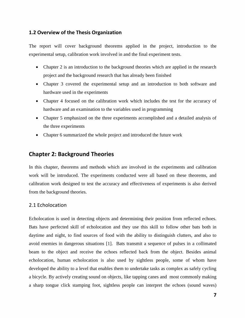
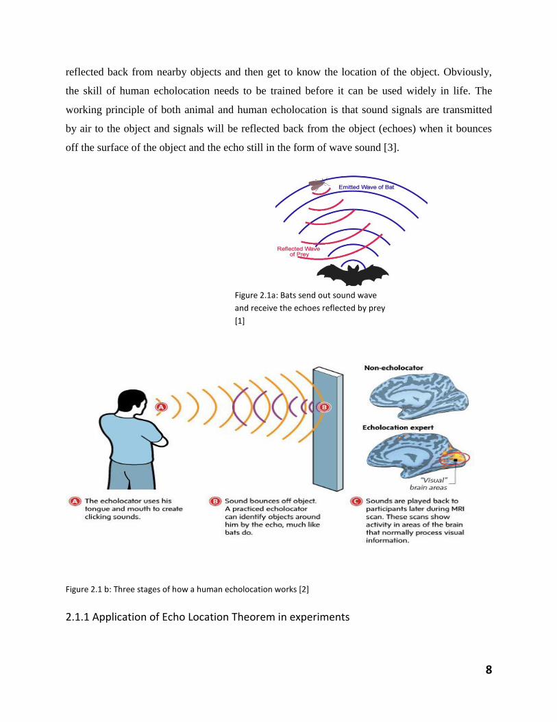
Figure 2.1a: Bats send out sound wave
and receive the echoes reflected by prey
[1]
reflected back from nearby objects and then get to know the location of the object. Obviously,
the skill of human echolocation needs to be trained before it can be used widely in life. The
working principle of both animal and human echolocation is that sound signals are transmitted
by air to the object and signals will be reflected back from the object (echoes) when it bounces
off the surface of the object and the echo still in the form of wave sound [3].
Figure 2.1 b: Three stages of how a human echolocation works [2]
2.1.1 Application of Echo Location Theorem in experiments
9
The ultrasonic sensor of the Lego NXT robot works based on the theorem of echo location,
which will be concretely introduced in section 3.1.1. Different from normal sound wave, the
ultrasonic sensor sends out a beam of ultrasound wave of which the sound range is out of human
being’s hearing range. The ultrasonic sensor locates where the object is through measuring the
time delay, and hence the distance, from the robot to the detected object.
2.2 Differences between sound and radio wave Echolocation working principles
Echolocation using radio waves gave rise the now well established technology of radar. Radars
are widely used in aircraft and other vehicles, as well as ground stations, to detect targets in the
local environment. Note that the use of word target to describe the items detected by the radar
comes from its historic roots in military use and is not meant to imply that all radars are designed
with the aim of shooting something down. The radio wave is a form of electromagnetic energy,
just as light wave are. Conversely, sound wave are the flow of acoustic energy. The key
difference between echolocation used sound and radio waves is the frequency of radio wave is
much higher than that of sound wave for the reason that light speed is 300,000,000 m/s, while the
sound speed is only 340 m/s. When measuring the distance to the target using echolocation the
radar measures the round trip time of the signal it transmits, i.e. how long it takes the signal to
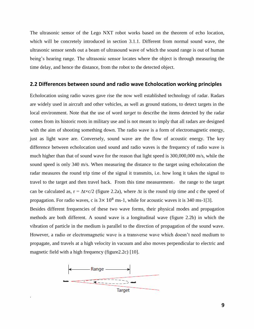
travel to the target and then travel back. From this time measurement, the range to the target
can be calculated as, r = ∆t×c/2 (figure 2.2a), where ∆t is the round trip time and c the speed of
propagation. For radio waves, c is 3× 10⁸ ms-1, while for acoustic waves it is 340 ms-1[3].
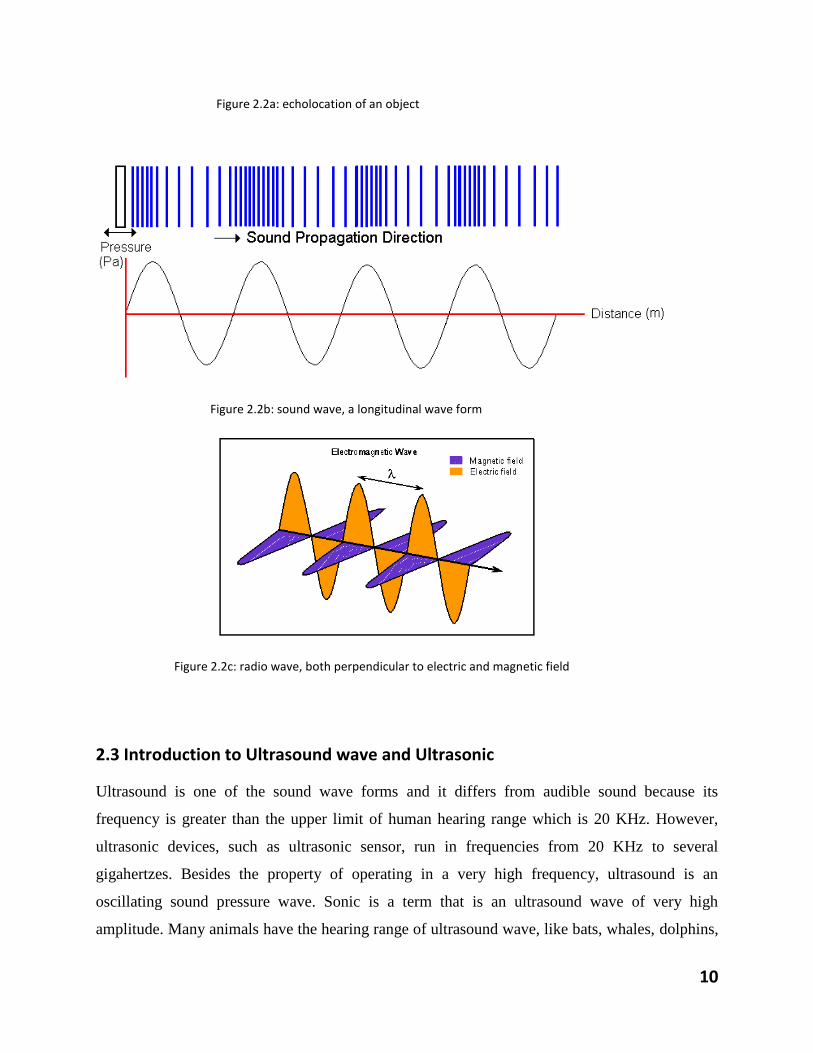
Besides different frequencies of these two wave forms, their physical modes and propagation
methods are both different. A sound wave is a longitudinal wave (figure 2.2b) in which the
vibration of particle in the medium is parallel to the direction of propagation of the sound wave.
However, a radio or electromagnetic wave is a transverse wave which doesn’t need medium to
propagate, and travels at a high velocity in vacuum and also moves perpendicular to electric and
magnetic field with a high frequency (figure2.2c) [10].
.
10
Figure 2.2a: echolocation of an object
Figure 2.2b: sound wave, a longitudinal wave form
Figure 2.2c: radio wave, both perpendicular to electric and magnetic field
2.3 Introduction to Ultrasound wave and Ultrasonic
Ultrasound is one of the sound wave forms and it differs from audible sound because its
frequency is greater than the upper limit of human hearing range which is 20 KHz. However,
ultrasonic devices, such as ultrasonic sensor, run in frequencies from 20 KHz to several
gigahertzes. Besides the property of operating in a very high frequency, ultrasound is an
oscillating sound pressure wave. Sonic is a term that is an ultrasound wave of very high
amplitude. Many animals have the hearing range of ultrasound wave, like bats, whales, dolphins,
11
etc. Ultrasonic can be widely applied to may fields, such as objects detection, distance
measurement, medical image, substance change of chemical properties, etc.
2.4 Echoic Flow Theorem
𝜏(𝑟) = 𝑟/𝑟̇ (1)
The concept of optical flow is more common than that of echoic flow. For cognitive radar
sensors, the simplest way to define echoic flow is the ration of range to rate of range,𝜏(𝑟) =
𝑟/𝑟̇ , where τ is echoic flow, r is the range to a detected object and �̇� is the change in range
between the current and previous measurement, and �̇� =𝑑𝑟
𝑑𝑡 which can also be seen as the
velocity of the moving object [16]. Therefore, echoic flow provides a direct way to measure the
time of radar system and detected object to collide with each other and τ has units of time. For
example, when a radar sensor system is moving in a speed of 10 m/s, and the range between the
radar system and the detected object is 60 m; the echoic flow τ is 6 s which means the time to
collision is 6s. The time derivative of echoic flow, ṫ(r), measures the intensity of the collision
and it is a dimensionless quantity. Radar echoic flow is based on the optical flow which
represents the pattern of current movement of objects in a visual scene caused by the relative
motion between the observer and the scene [17]. Optical flow can be measured as the change in
intensity and it can be calculated as the ratio of received intensity and change in intensity over an
interval of time. The optical flow τ means how long it takes for objects in relative motion to
collide [18]. Optical flow can be both applied to acoustic and electromagnetic sensing. For
example, bats use acoustic echolocation to navigate their path to find home and also to detect
enemies in the daytime and dark by applying echoic flow. Radar system use electromagnetic
waves to echolocate the target object. During the autonomous navigation of radar, echoic flow
can best help radar system to accurately detect the obstacles in front, and track and avoid them.
2.4.1 Application of Echoic Flow Theorem in experiments
𝜏 (r) =𝑟
𝑟̇ =
𝑟2
(𝑟2−𝑟1)/∆𝑡(2)
12
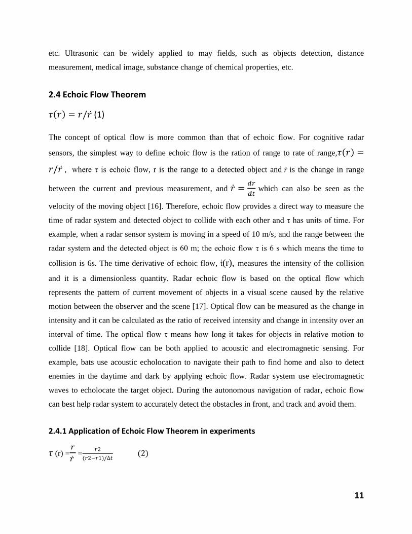
When using ultrasonic sensor to measure the range between the robot and the object, the echoic
flow τ(r) which is the time to collision can also be computed as the ratio of range to the velocity.
Since the robot is in the linear uniform motion, the velocity can be calculated in advance by
measuring the range by tape and recording the time the robot takes to approach the object. Then,
when a robot is approaching the object, the echoic flow can be computed continuously by using
the equation (1), showed in figure 2.4.1a. Another way to compute echoic flow τ is τ(r) =𝑟
𝑟̇
=𝑟2
(𝑟2−𝑟1)/∆𝑡 (2), where r2 is the current measured range and r1 is the range measured at last
time, ∆t=t2-t1 is the time interval between r2 and r1, and (r2-r1)/∆t indicates the current velocity
of the robot.
Figure 2.4.1a: when the robot is approaching to an object, the echoic flow can be computed by knowing the
velocity and the range
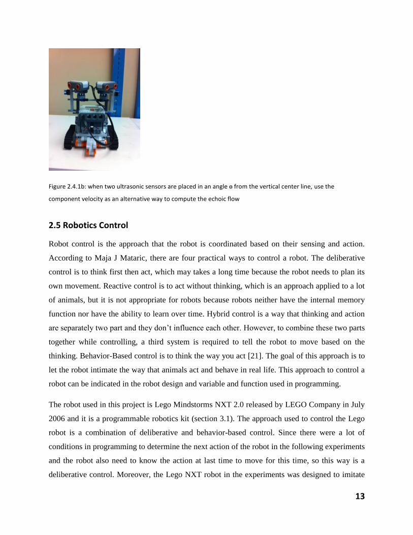
When two ultrasonic sensors are used and they are both placed in ө degrees from the vertical line
respectively (figure 2.4.1b). Since the robot is running forward, the component velocity v*cos (ө)
will be used to compute echoic flow, τ(r) = 𝑟
𝑣∗cos(ө) (3)
Echoic flow τ (time to collision) =R/V
Lego Robot with
a velocity V Range R
Ultrasonic sensor
13
Figure 2.4.1b: when two ultrasonic sensors are placed in an angle ө from the vertical center line, use the
component velocity as an alternative way to compute the echoic flow
2.5 Robotics Control
Robot control is the approach that the robot is coordinated based on their sensing and action.
According to Maja J Mataric, there are four practical ways to control a robot. The deliberative
control is to think first then act, which may takes a long time because the robot needs to plan its
own movement. Reactive control is to act without thinking, which is an approach applied to a lot
of animals, but it is not appropriate for robots because robots neither have the internal memory
function nor have the ability to learn over time. Hybrid control is a way that thinking and action
are separately two part and they don’t influence each other. However, to combine these two parts
together while controlling, a third system is required to tell the robot to move based on the
thinking. Behavior-Based control is to think the way you act [21]. The goal of this approach is to
let the robot intimate the way that animals act and behave in real life. This approach to control a
robot can be indicated in the robot design and variable and function used in programming.
The robot used in this project is Lego Mindstorms NXT 2.0 released by LEGO Company in July
2006 and it is a programmable robotics kit (section 3.1). The approach used to control the Lego
robot is a combination of deliberative and behavior-based control. Since there were a lot of
conditions in programming to determine the next action of the robot in the following experiments
and the robot also need to know the action at last time to move for this time, so this way is a
deliberative control. Moreover, the Lego NXT robot in the experiments was designed to imitate
14
the cars in real life which the two front wheels connected to one motor are for turning and the
two back wheels are only for moving, and the variables in MATLAB function to control the
robot also have practical meaning, like speed, and turning angle.
2.6 Linear Regression
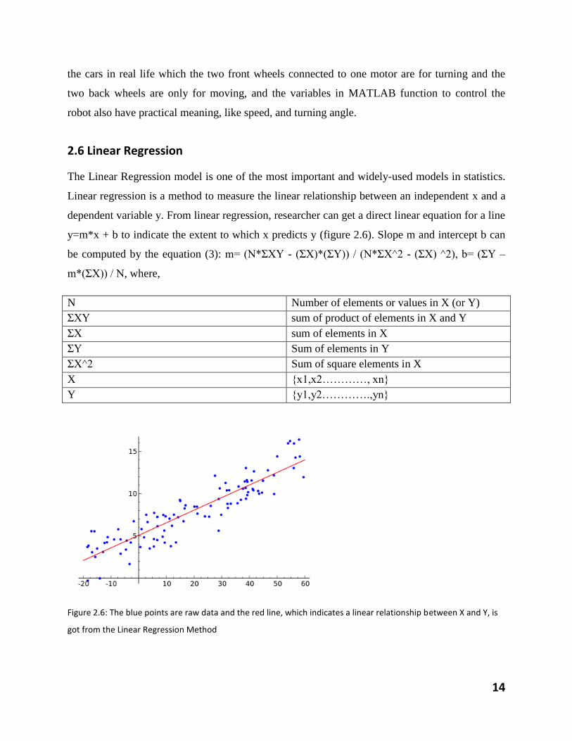
The Linear Regression model is one of the most important and widely-used models in statistics.
Linear regression is a method to measure the linear relationship between an independent x and a
dependent variable y. From linear regression, researcher can get a direct linear equation for a line
y=m*x + b to indicate the extent to which x predicts y (figure 2.6). Slope m and intercept b can
be computed by the equation (3): m= (N*ΣXY - (ΣX)*(ΣY)) / (N*ΣX^2 - (ΣX) ^2), b= (ΣY –
m*(ΣX)) / N, where,
N Number of elements or values in X (or Y)
ΣXY sum of product of elements in X and Y
ΣX sum of elements in X
ΣY Sum of elements in Y
ΣX^2 Sum of square elements in X
X {x1,x2…………, xn}
Y {y1,y2………….,yn}
Figure 2.6: The blue points are raw data and the red line, which indicates a linear relationship between X and Y, is
got from the Linear Regression Method
15
The method of linear regression will be applied to get an ideal estimated relationship between
range measured by ultrasonic sensor and the time it used. Details are introduced in chapter 4.1
testing the Buffer-size.
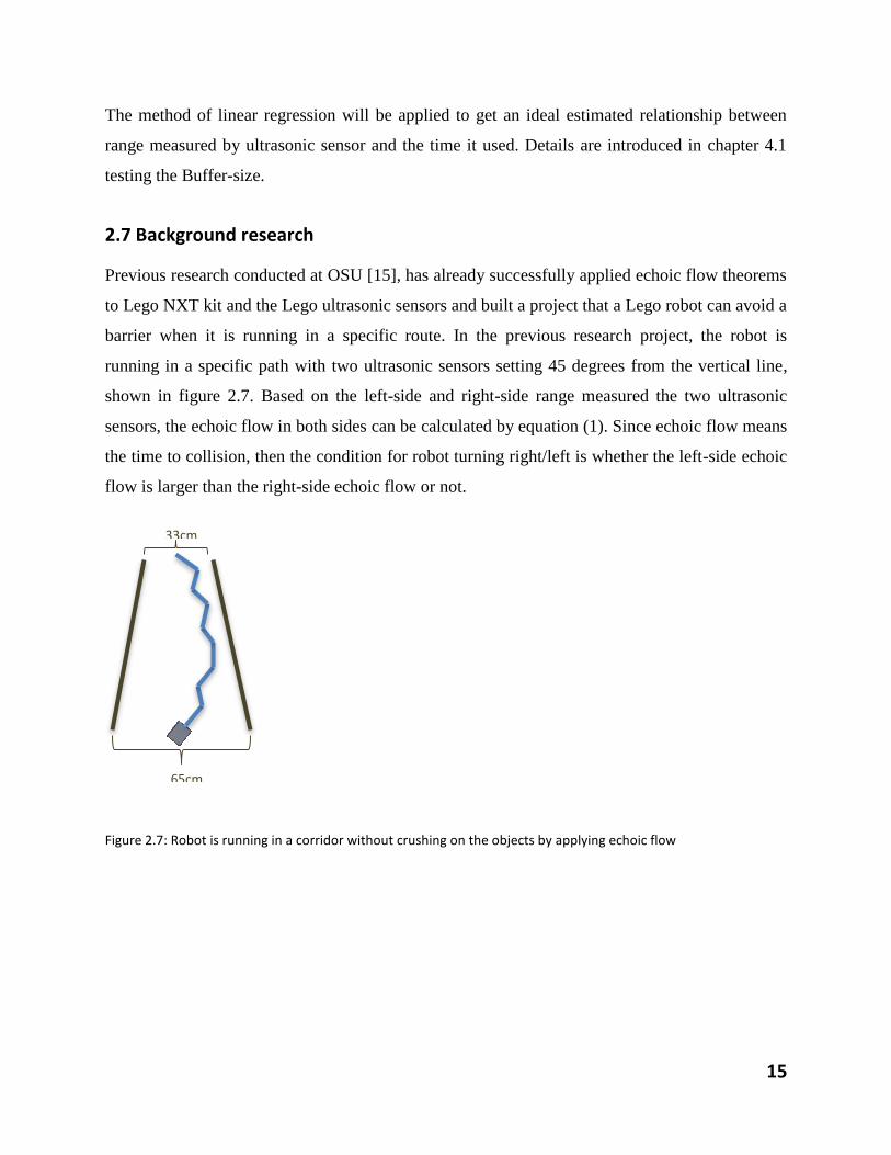
2.7 Background research
Previous research conducted at OSU [15], has already successfully applied echoic flow theorems
to Lego NXT kit and the Lego ultrasonic sensors and built a project that a Lego robot can avoid a
barrier when it is running in a specific route. In the previous research project, the robot is
running in a specific path with two ultrasonic sensors setting 45 degrees from the vertical line,
shown in figure 2.7. Based on the left-side and right-side range measured the two ultrasonic
sensors, the echoic flow in both sides can be calculated by equation (1). Since echoic flow means
the time to collision, then the condition for robot turning right/left is whether the left-side echoic
flow is larger than the right-side echoic flow or not.
Figure 2.7: Robot is running in a corridor without crushing on the objects by applying echoic flow
33cm
65cm
16
Chapter 3: Introduction to equipment and setup
Chapter 3 introduces the experiment setup and facilities used in experiments. Hardware in
experiment setup includes Lego NXT programmable kit, two ultrasonic sensors, three serve
motors and a USB connection wire. Software part consists of MATLAB 2012 (32 bit), Lego
Phantom driver and MATLAB Lego NXT toolbox.
3.1 Hardwire: Lego Mindstorms NXT 2.0
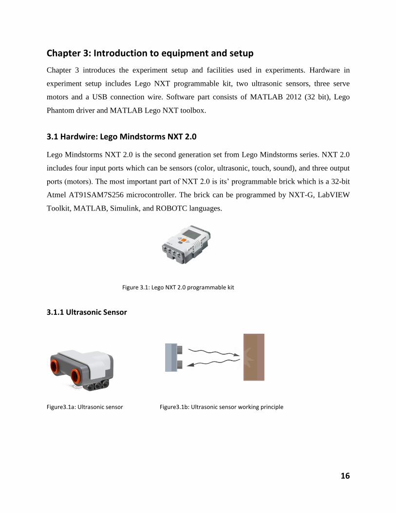
Lego Mindstorms NXT 2.0 is the second generation set from Lego Mindstorms series. NXT 2.0
includes four input ports which can be sensors (color, ultrasonic, touch, sound), and three output
ports (motors). The most important part of NXT 2.0 is its’ programmable brick which is a 32-bit
Atmel AT91SAM7S256 microcontroller. The brick can be programmed by NXT-G, LabVIEW
Toolkit, MATLAB, Simulink, and ROBOTC languages.
Figure 3.1: Lego NXT 2.0 programmable kit
3.1.1 Ultrasonic Sensor
Figure3.1a: Ultrasonic sensor Figure3.1b: Ultrasonic sensor working principle
17
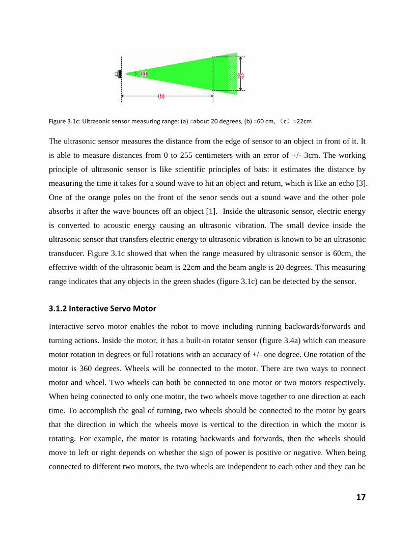
Figure 3.1c: Ultrasonic sensor measuring range: (a) =about 20 degrees, (b) =60 cm, (c)=22cm
The ultrasonic sensor measures the distance from the edge of sensor to an object in front of it. It
is able to measure distances from 0 to 255 centimeters with an error of +/- 3cm. The working
principle of ultrasonic sensor is like scientific principles of bats: it estimates the distance by
measuring the time it takes for a sound wave to hit an object and return, which is like an echo [3].
One of the orange poles on the front of the senor sends out a sound wave and the other pole
absorbs it after the wave bounces off an object [1]. Inside the ultrasonic sensor, electric energy
is converted to acoustic energy causing an ultrasonic vibration. The small device inside the
ultrasonic sensor that transfers electric energy to ultrasonic vibration is known to be an ultrasonic
transducer. Figure 3.1c showed that when the range measured by ultrasonic sensor is 60cm, the
effective width of the ultrasonic beam is 22cm and the beam angle is 20 degrees. This measuring
range indicates that any objects in the green shades (figure 3.1c) can be detected by the sensor.
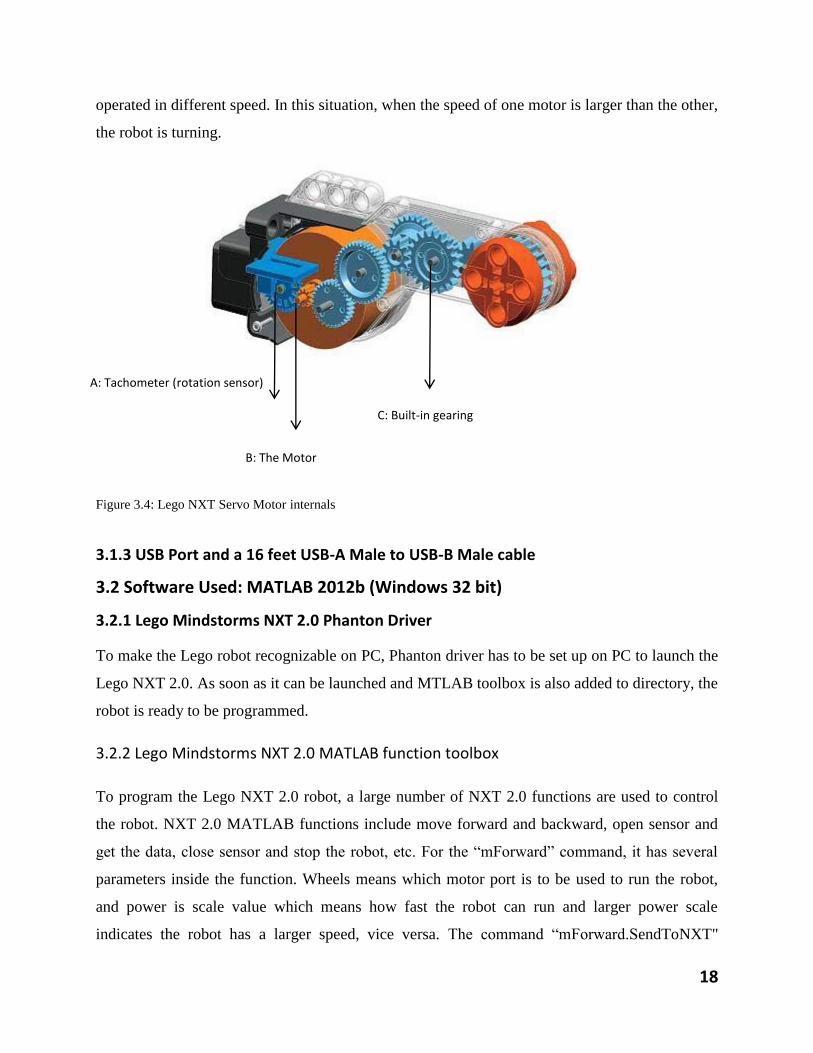
3.1.2 Interactive Servo Motor
Interactive servo motor enables the robot to move including running backwards/forwards and
turning actions. Inside the motor, it has a built-in rotator sensor (figure 3.4a) which can measure
motor rotation in degrees or full rotations with an accuracy of +/- one degree. One rotation of the
motor is 360 degrees. Wheels will be connected to the motor. There are two ways to connect
motor and wheel. Two wheels can both be connected to one motor or two motors respectively.
When being connected to only one motor, the two wheels move together to one direction at each
time. To accomplish the goal of turning, two wheels should be connected to the motor by gears
that the direction in which the wheels move is vertical to the direction in which the motor is
rotating. For example, the motor is rotating backwards and forwards, then the wheels should
move to left or right depends on whether the sign of power is positive or negative. When being
connected to different two motors, the two wheels are independent to each other and they can be
18
operated in different speed. In this situation, when the speed of one motor is larger than the other,
the robot is turning.
Figure 3.4: Lego NXT Servo Motor internals
3.1.3 USB Port and a 16 feet USB-A Male to USB-B Male cable
3.2 Software Used: MATLAB 2012b (Windows 32 bit)
3.2.1 Lego Mindstorms NXT 2.0 Phanton Driver
To make the Lego robot recognizable on PC, Phanton driver has to be set up on PC to launch the
Lego NXT 2.0. As soon as it can be launched and MTLAB toolbox is also added to directory, the
robot is ready to be programmed.
3.2.2 Lego Mindstorms NXT 2.0 MATLAB function toolbox
To program the Lego NXT 2.0 robot, a large number of NXT 2.0 functions are used to control
the robot. NXT 2.0 MATLAB functions include move forward and backward, open sensor and
get the data, close sensor and stop the robot, etc. For the “mForward” command, it has several
parameters inside the function. Wheels means which motor port is to be used to run the robot,
and power is scale value which means how fast the robot can run and larger power scale
indicates the robot has a larger speed, vice versa. The command “mForward.SendToNXT"
A: Tachometer (rotation sensor)
B: The Motor
C: Built-in gearing
19
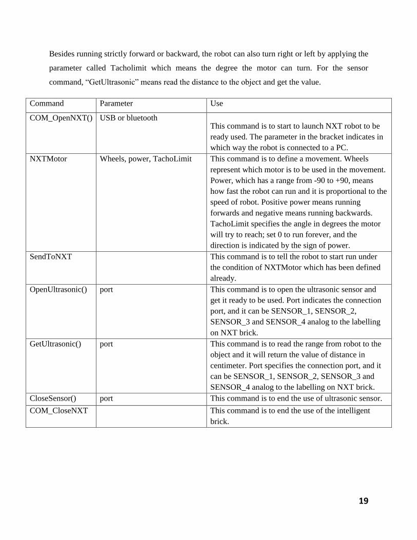
Besides running strictly forward or backward, the robot can also turn right or left by applying the
parameter called Tacholimit which means the degree the motor can turn. For the sensor
command, “GetUltrasonic” means read the distance to the object and get the value.
Command Parameter Use
COM_OpenNXT() USB or bluetooth This command is to start to launch NXT robot to be
ready used. The parameter in the bracket indicates in
which way the robot is connected to a PC.
NXTMotor Wheels, power, TachoLimit This command is to define a movement. Wheels
represent which motor is to be used in the movement.
Power, which has a range from -90 to +90, means
how fast the robot can run and it is proportional to the
speed of robot. Positive power means running
forwards and negative means running backwards.
TachoLimit specifies the angle in degrees the motor
will try to reach; set 0 to run forever, and the
direction is indicated by the sign of power.
SendToNXT This command is to tell the robot to start run under
the condition of NXTMotor which has been defined
already.
OpenUltrasonic() port This command is to open the ultrasonic sensor and
get it ready to be used. Port indicates the connection
port, and it can be SENSOR_1, SENSOR_2,
SENSOR_3 and SENSOR_4 analog to the labelling
on NXT brick.
GetUltrasonic() port This command is to read the range from robot to the
object and it will return the value of distance in
centimeter. Port specifies the connection port, and it
can be SENSOR_1, SENSOR_2, SENSOR_3 and
SENSOR_4 analog to the labelling on NXT brick.
CloseSensor() port This command is to end the use of ultrasonic sensor.
COM_CloseNXT This command is to end the use of the intelligent
brick.
20
Chapter 4: Calibration of Lego Sensors
In this chapter, calibration activities which were conducted before implementing the experiments
will be discussed. The calibration work includes testing the most appropriate value for buffer-
size, calibrating two sensors when they work together and determining the most appropriate
value of angle in which the sensor and robot should be set. Methods used in calibration work and
conclusion got from the results are also introduced in this chapter.
4.1 The need for calibration in experiments
Before undertaking three experiments, calibration was required to ensure these experiments are
done in best situations where there are no hardware problems or environmental influences.
Different kinds of factors may influence the accomplishment of experiments, such as
environmental noise to the measurement of ultrasonic sensor, logic error in MATLAB scripts,
interaction influences when two ultrasonic sensors work together abreast, low battery influences
to Lego robot, etc. One of the most important objectives of doing calibration work before putting
a lot of efforts to experiments is to know how these factors will influence the result of each
experiment and how to make corrections to avoid the unwanted results.
4.2 Ultrasonic sensor range measurement
The maximum speed for a regular NXT robot is about 1-2 m/s, and the ultrasound travels with
330 meters per second through air. Since ultrasound travels a lot faster than the robot motor does,
there will be a freeze-frame snapshot of the current range from the sensor to the object. Freeze-
frame snapshot will make the robot looks like stationary from the MATLAB graph, because the
range measured by ultrasonic sensor for the current time will be as almost same as the range
measured in next time, which means the range measured by ultrasonic sensor merely change
during a small interval of time. For example, an obvious change in range in MATLAB graph
takes 1s, but the ultrasonic senor will measure 50 values of range in 1 second. This situation is
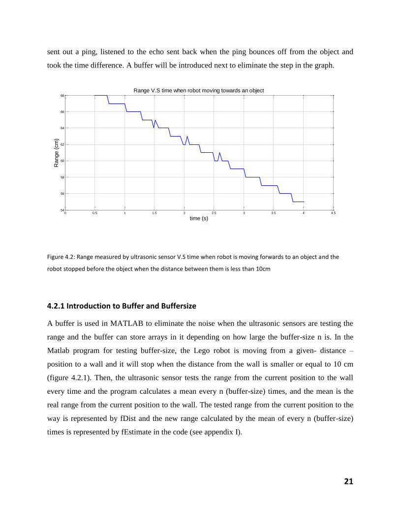
showed in the graph below (figure 4.2). From the graph, we can see that the range (y axis)
showed step sized line instead of continuous smooth line, which indicates the range keeps
unchanged during a small time interval. During this freeze-frame snapshot, the ultrasonic sensor
21
sent out a ping, listened to the echo sent back when the ping bounces off from the object and
took the time difference. A buffer will be introduced next to eliminate the step in the graph.
Figure 4.2: Range measured by ultrasonic sensor V.S time when robot is moving forwards to an object and the
robot stopped before the object when the distance between them is less than 10cm
4.2.1 Introduction to Buffer and Buffersize
A buffer is used in MATLAB to eliminate the noise when the ultrasonic sensors are testing the
range and the buffer can store arrays in it depending on how large the buffer-size n is. In the
Matlab program for testing buffer-size, the Lego robot is moving from a given- distance –
position to a wall and it will stop when the distance from the wall is smaller or equal to 10 cm
(figure 4.2.1). Then, the ultrasonic sensor tests the range from the current position to the wall
every time and the program calculates a mean every n (buffer-size) times, and the mean is the
real range from the current position to the wall. The tested range from the current position to the
way is represented by fDist and the new range calculated by the mean of every n (buffer-size)
times is represented by fEstimate in the code (see appendix I).
0 0.5 1 1.5 2 2.5 3 3.5 4 4.554
56
58
60
62
64
66
68
time (s)
Range (
cm
)
Range V.S time when robot moving towards an object
22
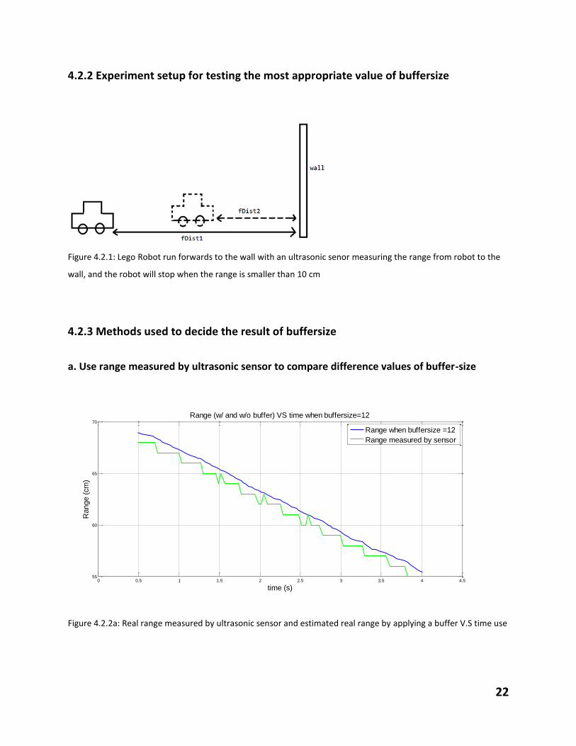
4.2.2 Experiment setup for testing the most appropriate value of buffersize
Figure 4.2.1: Lego Robot run forwards to the wall with an ultrasonic senor measuring the range from robot to the
wall, and the robot will stop when the range is smaller than 10 cm
4.2.3 Methods used to decide the result of buffersize
a. Use range measured by ultrasonic sensor to compare difference values of buffer-size
Figure 4.2.2a: Real range measured by ultrasonic sensor and estimated real range by applying a buffer V.S time use
0 0.5 1 1.5 2 2.5 3 3.5 4 4.555
60
65
70
time (s)
Range (
cm
)
Range (w/ and w/o buffer) VS time when buffersize=12
Range when buffersize =12
Range measured by sensor
23
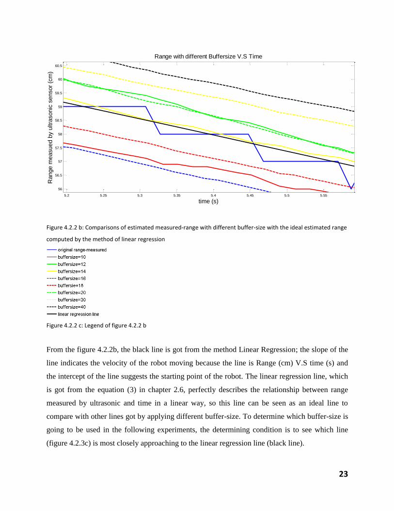
Figure 4.2.2 b: Comparisons of estimated measured-range with different buffer-size with the ideal estimated range
computed by the method of linear regression
Figure 4.2.2 c: Legend of figure 4.2.2 b
From the figure 4.2.2b, the black line is got from the method Linear Regression; the slope of the
line indicates the velocity of the robot moving because the line is Range (cm) V.S time (s) and
the intercept of the line suggests the starting point of the robot. The linear regression line, which
is got from the equation (3) in chapter 2.6, perfectly describes the relationship between range
measured by ultrasonic and time in a linear way, so this line can be seen as an ideal line to
compare with other lines got by applying different buffer-size. To determine which buffer-size is
going to be used in the following experiments, the determining condition is to see which line
(figure 4.2.3c) is most closely approaching to the linear regression line (black line).
5.2 5.25 5.3 5.35 5.4 5.45 5.5 5.55
56
56.5
57
57.5
58
58.5
59
59.5
60
60.5
time (s)
Range m
easued b
y u
ltra
sonic
sensor
(cm
)Range with different Buffersize V.S Time
24
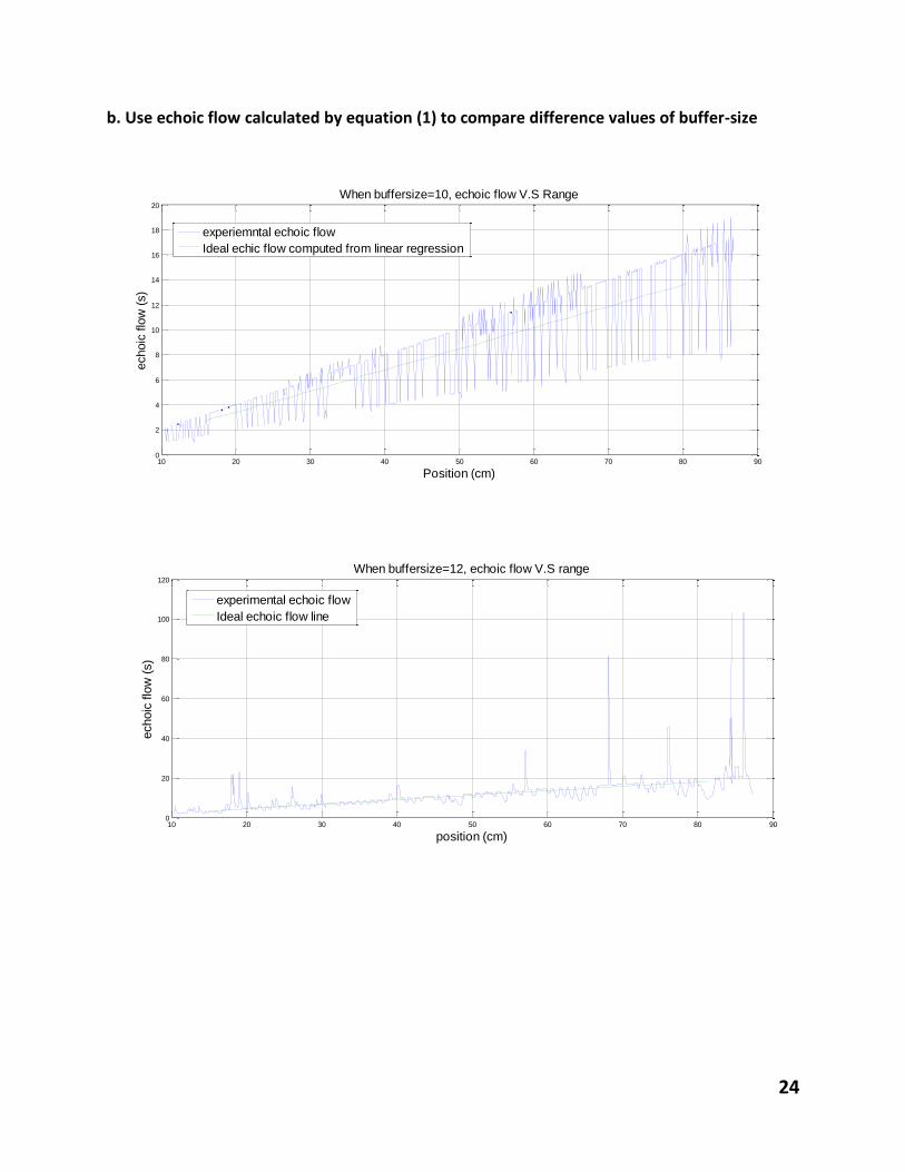
b. Use echoic flow calculated by equation (1) to compare difference values of buffer-size
10 20 30 40 50 60 70 80 900
2
4
6
8
10
12
14
16
18
20
Position (cm)
echoic
flo
w (
s)
When buffersize=10, echoic flow V.S Range
experiemntal echoic flow
Ideal echic flow computed from linear regression
10 20 30 40 50 60 70 80 900
20
40
60
80
100
120
When buffersize=12, echoic flow V.S range
position (cm)
echoic
flo
w (
s)
experimental echoic flow
Ideal echoic flow line
25
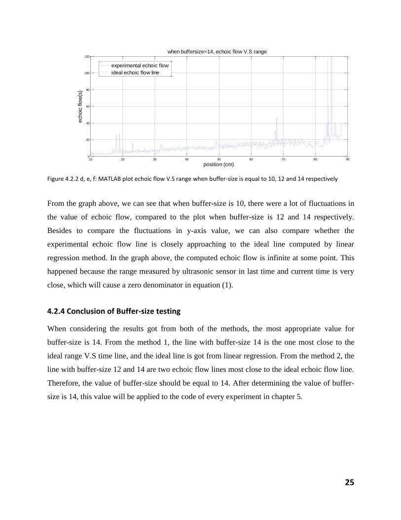
Figure 4.2.2 d, e, f: MATLAB plot echoic flow V.S range when buffer-size is equal to 10, 12 and 14 respectively
From the graph above, we can see that when buffer-size is 10, there were a lot of fluctuations in
the value of echoic flow, compared to the plot when buffer-size is 12 and 14 respectively.
Besides to compare the fluctuations in y-axis value, we can also compare whether the
experimental echoic flow line is closely approaching to the ideal line computed by linear
regression method. In the graph above, the computed echoic flow is infinite at some point. This
happened because the range measured by ultrasonic sensor in last time and current time is very
close, which will cause a zero denominator in equation (1).
4.2.4 Conclusion of Buffer-size testing
When considering the results got from both of the methods, the most appropriate value for
buffer-size is 14. From the method 1, the line with buffer-size 14 is the one most close to the
ideal range V.S time line, and the ideal line is got from linear regression. From the method 2, the
line with buffer-size 12 and 14 are two echoic flow lines most close to the ideal echoic flow line.
Therefore, the value of buffer-size should be equal to 14. After determining the value of buffer-
size is 14, this value will be applied to the code of every experiment in chapter 5.
10 20 30 40 50 60 70 80 900
20
40
60
80
100
120
when buffersize=14, echoic flow V.S range
position (cm)
echoic
flo
w(s
)
experimental echoic flow
ideal echoic flow line
26
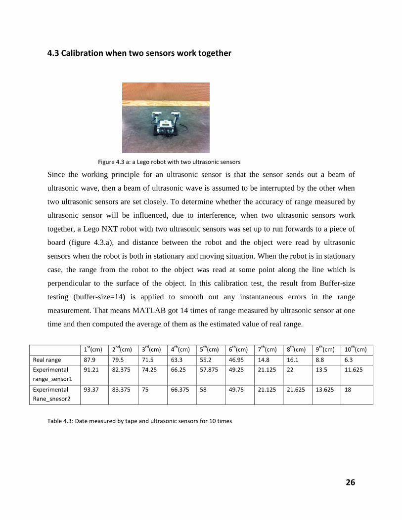
4.3 Calibration when two sensors work together
Figure 4.3 a: a Lego robot with two ultrasonic sensors
Since the working principle for an ultrasonic sensor is that the sensor sends out a beam of
ultrasonic wave, then a beam of ultrasonic wave is assumed to be interrupted by the other when
two ultrasonic sensors are set closely. To determine whether the accuracy of range measured by
ultrasonic sensor will be influenced, due to interference, when two ultrasonic sensors work
together, a Lego NXT robot with two ultrasonic sensors was set up to run forwards to a piece of
board (figure 4.3.a), and distance between the robot and the object were read by ultrasonic
sensors when the robot is both in stationary and moving situation. When the robot is in stationary
case, the range from the robot to the object was read at some point along the line which is
perpendicular to the surface of the object. In this calibration test, the result from Buffer-size
testing (buffer-size=14) is applied to smooth out any instantaneous errors in the range
measurement. That means MATLAB got 14 times of range measured by ultrasonic sensor at one
time and then computed the average of them as the estimated value of real range.
1st
(cm) 2nd
(cm) 3rd
(cm) 4th
(cm) 5th
(cm) 6th
(cm) 7th
(cm) 8th
(cm) 9th
(cm) 10th
(cm)
Real range 87.9 79.5 71.5 63.3 55.2 46.95 14.8 16.1 8.8 6.3
Experimental
range_sensor1
91.21 82.375 74.25 66.25 57.875 49.25 21.125 22 13.5 11.625
Experimental
Rane_snesor2
93.37 83.375 75 66.375 58 49.75 21.125 21.625 13.625 18
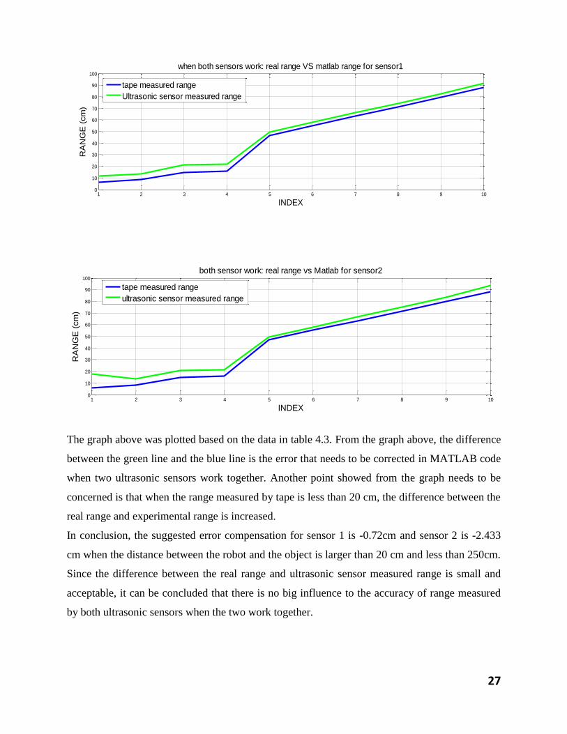
Table 4.3: Date measured by tape and ultrasonic sensors for 10 times
27
The graph above was plotted based on the data in table 4.3. From the graph above, the difference
between the green line and the blue line is the error that needs to be corrected in MATLAB code
when two ultrasonic sensors work together. Another point showed from the graph needs to be
concerned is that when the range measured by tape is less than 20 cm, the difference between the
real range and experimental range is increased.
In conclusion, the suggested error compensation for sensor 1 is -0.72cm and sensor 2 is -2.433
cm when the distance between the robot and the object is larger than 20 cm and less than 250cm.
Since the difference between the real range and ultrasonic sensor measured range is small and
acceptable, it can be concluded that there is no big influence to the accuracy of range measured
by both ultrasonic sensors when the two work together.
1 2 3 4 5 6 7 8 9 100
10
20
30
40
50
60
70
80
90
100
INDEX
RA
NG
E (
cm
)
when both sensors work: real range VS matlab range for sensor1
tape measured range
Ultrasonic sensor measured range
1 2 3 4 5 6 7 8 9 100
10
20
30
40
50
60
70
80
90
100
INDEX
RA
NG
E (
cm
)
both sensor work: real range vs Matlab for sensor2
tape measured range
ultrasonic sensor measured range
28
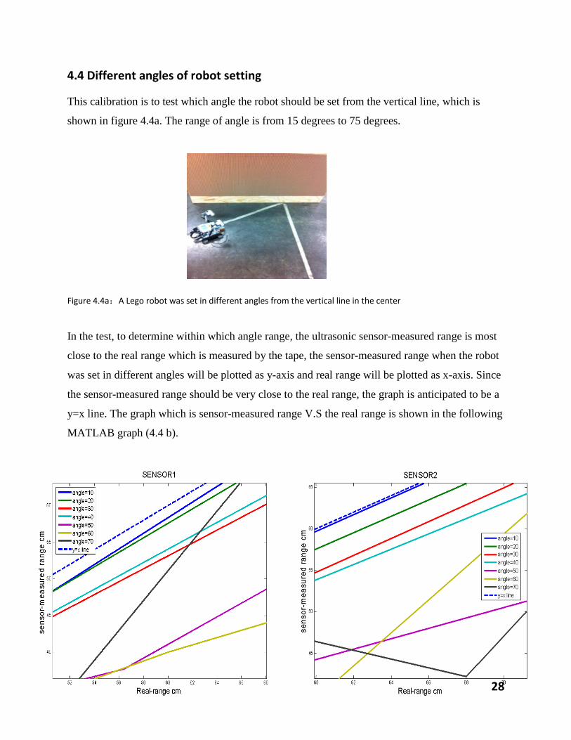
4.4 Different angles of robot setting
This calibration is to test which angle the robot should be set from the vertical line, which is
shown in figure 4.4a. The range of angle is from 15 degrees to 75 degrees.
Figure 4.4a:A Lego robot was set in different angles from the vertical line in the center
In the test, to determine within which angle range, the ultrasonic sensor-measured range is most
close to the real range which is measured by the tape, the sensor-measured range when the robot
was set in different angles will be plotted as y-axis and real range will be plotted as x-axis. Since
the sensor-measured range should be very close to the real range, the graph is anticipated to be a
y=x line. The graph which is sensor-measured range V.S the real range is shown in the following
MATLAB graph (4.4 b).
29
Figure 4.4b: Sensor-measured range V.S real range for both sensor 1 and sensor 2 when the sensors are
set in different angles from the central vertical line
From the graph, the blue dash line (y=x line) is the ideal situation where the range is measured
by the tape. All of lines where angle is equal to 10, 20, 30 and 40 degrees showed a linear
relationship between y-axis and x-axis, were parallel to each other and these lines are also close
to the ideal line (blue dash line). The lines where the angle is larger than 40 degrees are far from
the ideal line. Both sensor 1 and sensor 2 showed the same characteristics when comparing the
sensor-measured range to the real range.
Thus, it can be concluded that when angle is from 0◦ to 40◦, the sensor-measured range is much
closer to real range. This conclusion can be applied to experiment 3 and details will be
introduced in section 5.3.
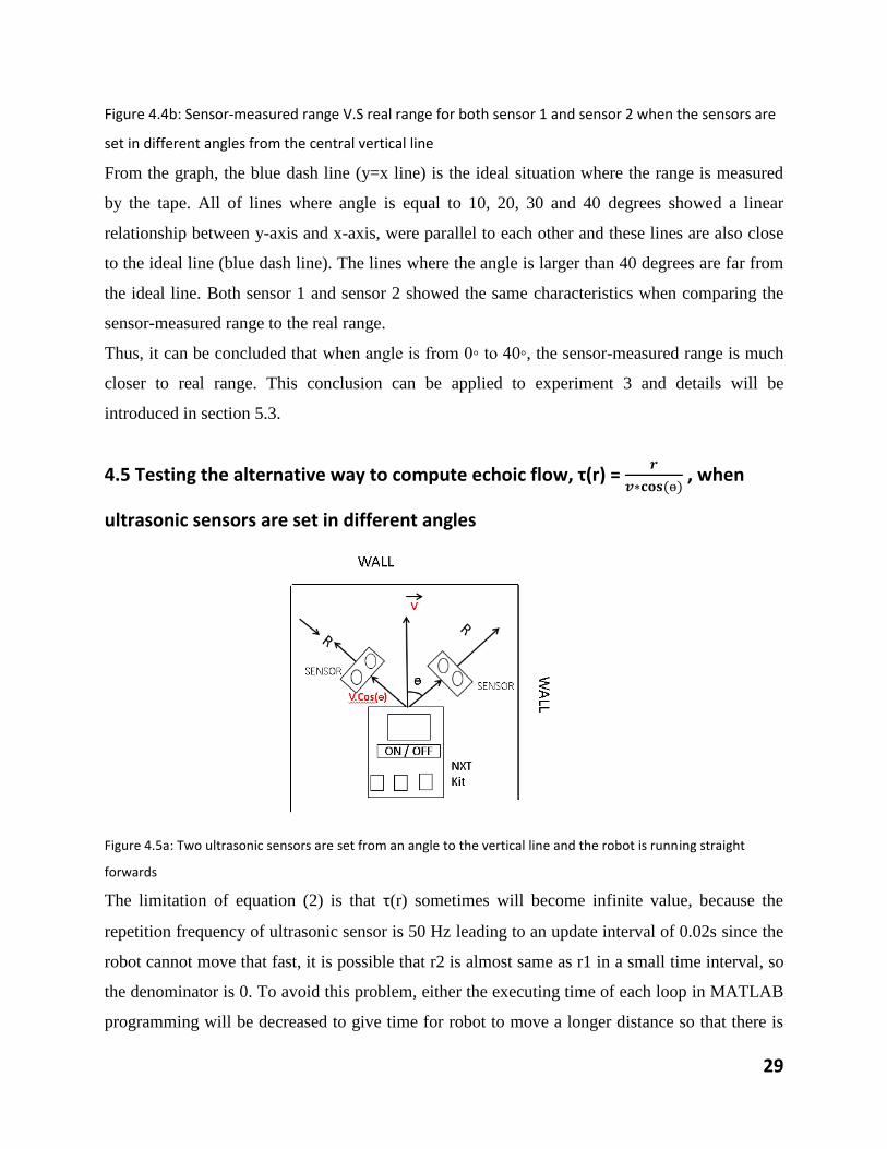
4.5 Testing the alternative way to compute echoic flow, τ(r) = 𝒓
𝒗∗𝐜𝐨𝐬(ө) , when
ultrasonic sensors are set in different angles
Figure 4.5a: Two ultrasonic sensors are set from an angle to the vertical line and the robot is running straight
forwards
The limitation of equation (2) is that τ(r) sometimes will become infinite value, because the
repetition frequency of ultrasonic sensor is 50 Hz leading to an update interval of 0.02s since the
robot cannot move that fast, it is possible that r2 is almost same as r1 in a small time interval, so
the denominator is 0. To avoid this problem, either the executing time of each loop in MATLAB
programming will be decreased to give time for robot to move a longer distance so that there is
30
an obvious difference between r2 and r1, or the ultrasonic sensor can be set in a position where
there is an angle from the vertical line (figure 4.5). When the two ultrasonic sensors are set in
such way, equation (3) can be applied to compute the echoic flow τ. The goal of flowing test is to
determine at which angle the ultrasonic sensor is set, the computed echoic flow by equation (3) is
most close to the real echoic flow. The echoic flow was computed by the equation:
time=𝒓𝒂𝒏𝒈𝒆
𝒅𝒊𝒓𝒆𝒄𝒕𝒊𝒐𝒏𝒗𝒆𝒍𝒐𝒄𝒊𝒕𝒚 . Range is the distance from the each of the sensor to the edge of right-side
and left-side object. The velocity can be computed in advance by knowing the time the robot
used to run in a given distance, v=s/t.
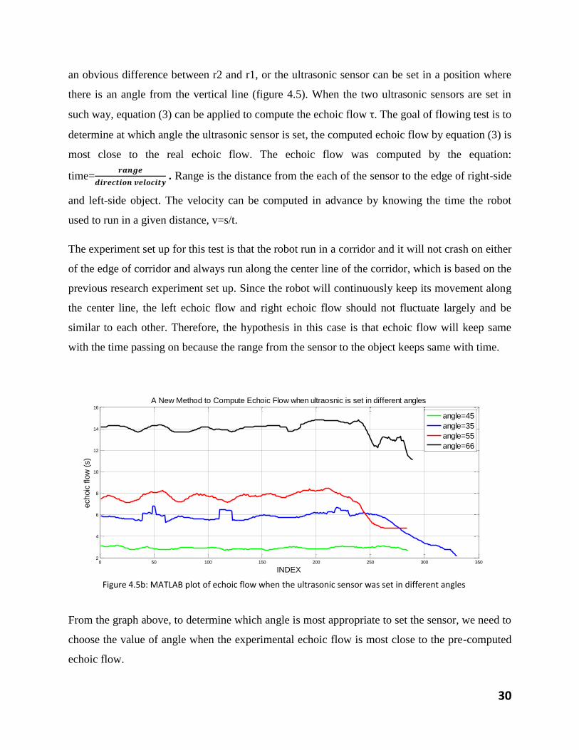
The experiment set up for this test is that the robot run in a corridor and it will not crash on either
of the edge of corridor and always run along the center line of the corridor, which is based on the
previous research experiment set up. Since the robot will continuously keep its movement along
the center line, the left echoic flow and right echoic flow should not fluctuate largely and be
similar to each other. Therefore, the hypothesis in this case is that echoic flow will keep same
with the time passing on because the range from the sensor to the object keeps same with time.
Figure 4.5b: MATLAB plot of echoic flow when the ultrasonic sensor was set in different angles
From the graph above, to determine which angle is most appropriate to set the sensor, we need to
choose the value of angle when the experimental echoic flow is most close to the pre-computed
echoic flow.
0 50 100 150 200 250 300 3502
4
6
8
10
12
14
16
INDEX
echoic
flo
w (
s)
A New Method to Compute Echoic Flow when ultraosnic is set in different angles
angle=45
angle=35
angle=55
angle=66
31
In conclusion, the angle of 45 degrees should be chosen. First, the green line in the figure 4.5b
(angle=45) is the most stable line because the standard deviation of data in this line is smaller
than 1.5, while the y-axis value (echoic flow) on other lines changed a lot with index. Ultimately,
the experimental echoic flow computed by MATLAB codes when the angle is 45 degrees was
about 3.125 s (average value), which is showed in figure 4.5b. The value of real echoic flow
calculated by the equation time is equal to distance over speed is about 3.035 s (average value).
Compared the real echoic flow and experimental echoic flow, angle that is equal to 45 degrees
should be chosen. In the following experiments, the ultrasonic sensors should be set in an angle
of 45 degrees if there is a need that the ultrasonic sensor should look left or right to read range.
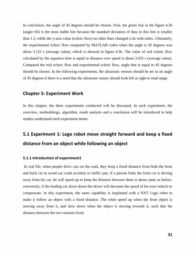
Chapter 5: Experiment Work
In this chapter, the three experiments conducted will be discussed. In each experiment, the
overview, methodology, algorithm, result analysis and a conclusion will be introduced to help
readers understand each experiment better.
5.1 Experiment 1: Lego robot move straight forward and keep a fixed
distance from an object while following an object
5.1.1 Introduction of experiment1
In real life, when people drive cars on the road, they keep a fixed distance from both the front
and back car to avoid car crash accident or traffic jam. If a person finds the front car is driving
away from his car, he will speed up to keep the distance between them is about same as before,
conversely, if the leading car slows down the driver will decrease the speed of his own vehicle to
compensate. In this experiment, the same capability is implanted with a NXT Lego robot to
make it follow an object with a fixed distance. The robot speed up when the front object is
moving away from it, and slow down when the object is moving towards it, such that the
distance between the two remains fixed.
32
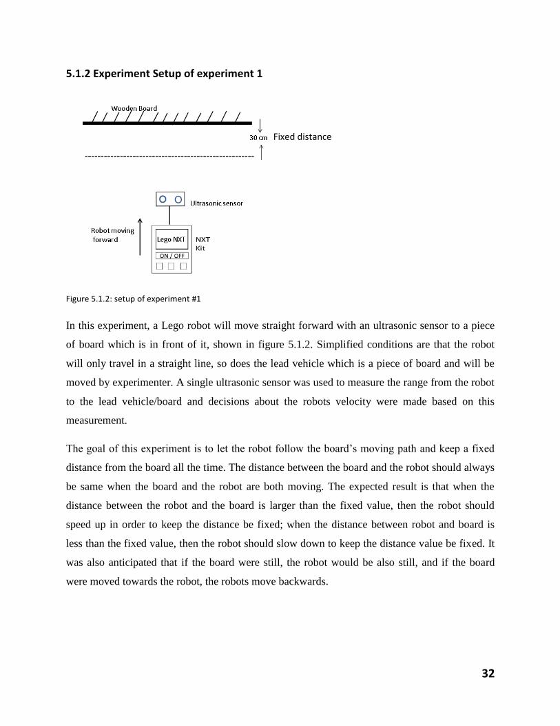
5.1.2 Experiment Setup of experiment 1
Figure 5.1.2: setup of experiment #1
In this experiment, a Lego robot will move straight forward with an ultrasonic sensor to a piece
of board which is in front of it, shown in figure 5.1.2. Simplified conditions are that the robot
will only travel in a straight line, so does the lead vehicle which is a piece of board and will be
moved by experimenter. A single ultrasonic sensor was used to measure the range from the robot
to the lead vehicle/board and decisions about the robots velocity were made based on this
measurement.
The goal of this experiment is to let the robot follow the board’s moving path and keep a fixed
distance from the board all the time. The distance between the board and the robot should always
be same when the board and the robot are both moving. The expected result is that when the
distance between the robot and the board is larger than the fixed value, then the robot should
speed up in order to keep the distance be fixed; when the distance between robot and board is
less than the fixed value, then the robot should slow down to keep the distance value be fixed. It
was also anticipated that if the board were still, the robot would be also still, and if the board
were moved towards the robot, the robots move backwards.
Fixed distance
33
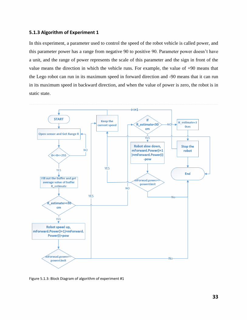
5.1.3 Algorithm of Experiment 1
In this experiment, a parameter used to control the speed of the robot vehicle is called power, and
this parameter power has a range from negative 90 to positive 90. Parameter power doesn’t have
a unit, and the range of power represents the scale of this parameter and the sign in front of the
value means the direction in which the vehicle runs. For example, the value of +90 means that
the Lego robot can run in its maximum speed in forward direction and -90 means that it can run
in its maximum speed in backward direction, and when the value of power is zero, the robot is in
static state.
Figure 5.1.3: Block Diagram of algorithm of experiment #1
34
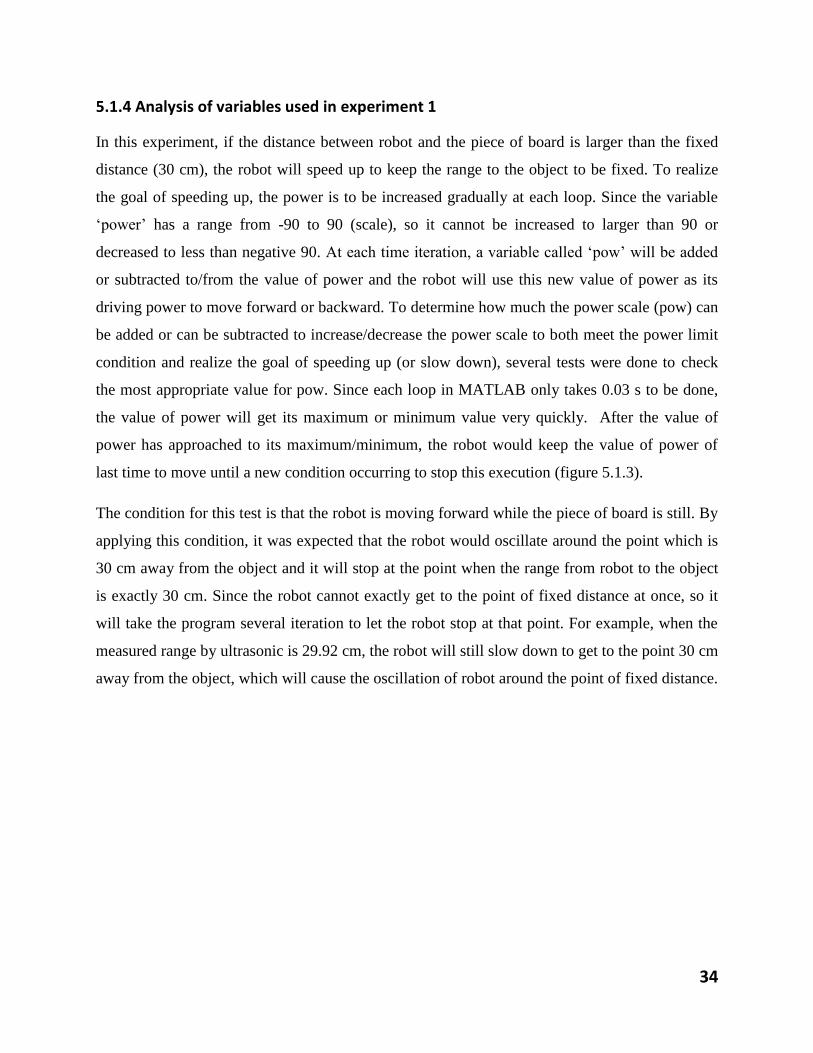
5.1.4 Analysis of variables used in experiment 1
In this experiment, if the distance between robot and the piece of board is larger than the fixed
distance (30 cm), the robot will speed up to keep the range to the object to be fixed. To realize
the goal of speeding up, the power is to be increased gradually at each loop. Since the variable
‘power’ has a range from -90 to 90 (scale), so it cannot be increased to larger than 90 or
decreased to less than negative 90. At each time iteration, a variable called ‘pow’ will be added
or subtracted to/from the value of power and the robot will use this new value of power as its
driving power to move forward or backward. To determine how much the power scale (pow) can
be added or can be subtracted to increase/decrease the power scale to both meet the power limit
condition and realize the goal of speeding up (or slow down), several tests were done to check
the most appropriate value for pow. Since each loop in MATLAB only takes 0.03 s to be done,
the value of power will get its maximum or minimum value very quickly. After the value of
power has approached to its maximum/minimum, the robot would keep the value of power of
last time to move until a new condition occurring to stop this execution (figure 5.1.3).
The condition for this test is that the robot is moving forward while the piece of board is still. By
applying this condition, it was expected that the robot would oscillate around the point which is
30 cm away from the object and it will stop at the point when the range from robot to the object
is exactly 30 cm. Since the robot cannot exactly get to the point of fixed distance at once, so it
will take the program several iteration to let the robot stop at that point. For example, when the
measured range by ultrasonic is 29.92 cm, the robot will still slow down to get to the point 30 cm
away from the object, which will cause the oscillation of robot around the point of fixed distance.
35
From these three graphs, when the value of POW is equal to 5, the robot is oscillating for a
longer time to get to the point and stop in the end, compared with graphs with POW=3 and
POW=7. When the POW is equal to 3 and 7, the time the robot takes to get to the end is same.
0 2 4 6 8 10 12 14 16-100
0
100
time (s)
Pow
er
(scale
)
Single Sensor condition, when Pow=3, power and range VS time
0 2 4 6 8 10 12 14 160
200
400
power
range
Range(cm)
0 5 10 15 20 25 30-100
-80
-60
-40
-20
0
20
40
60
80
100
time (s)
Pow
er
(scale
)
0 5 10 15 20 25 3020
30
40
50
60
70
80
90
100
110
120
Single sensor considtion, pow=5, Power and Range VS Time
Power
Range
Range(cm)
0 5 10 15-100
0
100
time (s)
pow
er
(scale
)
In single sensor condition, pow=7, Power and Range VS time
0 5 10 150
100
200
Power
range
Range(cm)
36
5.1.5 Future progress of experiment 1
In experiment 1, the range from the robot to the object is used as the variable to determine
whether the robot should speed up or slow down to keep the distance to the object be fixed every
time. Instead of using range to be the determinant, echoic flow which is the time to collision also
can be used as the determinant to decide whether to speed up or slow down. When calculating
the echoic flow, it is equal to range divides by the value of change in range over change in time,
𝜏(𝑟) = 𝑟/�̇� =r/V=r/(r2-r1)/(t2-t1)=r/(∆ r/∆t). Before do this test, echoic flow needs to be
calculated when the robot 30 centimeters away from the object (a piece of board). Then this
echoic flow will be the fixed value of time to collision𝜏_𝑓𝑖𝑥𝑒𝑑. If τ< τ_fixed, robot needs to
slow down, if τ>τ_fixed, robot should speed up.
5.1.6 Conclusion of Experiment 1
The robot with calibrated ultrasonic sensors can speed up when the distance from the robot to the
object is larger than the fixed distance, and it can also slow down when the distance to the object
is less than the fixed distance. Thus, the calibrated robot can keep a fixed distance to the object
which is a piece of board can be moved. The speed of the robot was controlled to realize the goal
of keeping the distance from sensor to the object be fixed all the time.
5.2 Experiment 2: A Lego robot moving forward with two ultrasonic sensors
following an object’s path
5.2.1 Introduction of Experiment 2
This experiment is an expansion upon experiment1. The setup of this experiment is basically
same with experiment 1 except that experiment 2 uses two ultrasonic sensors (figure 5.2.2). As
before, the sensors are used to measure the range from the robot to the object, which is a piece of
wooden board. Now, however, the data from the two sensors must be combined as part of the
decision making process. Both of ultrasonic sensors are set straightly forwards to the board, and
the robot can only move straightly forwards and backwards to/from the piece of board. The piece
of board can be also manually moved forwards and backwards by experimenter. Alternatively,
the piece of board can also be stationary.
37
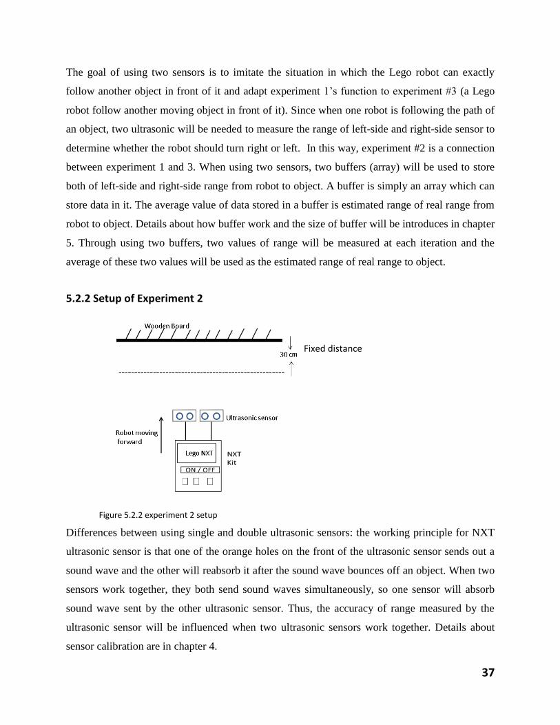
The goal of using two sensors is to imitate the situation in which the Lego robot can exactly
follow another object in front of it and adapt experiment 1’s function to experiment #3 (a Lego
robot follow another moving object in front of it). Since when one robot is following the path of
an object, two ultrasonic will be needed to measure the range of left-side and right-side sensor to
determine whether the robot should turn right or left. In this way, experiment #2 is a connection
between experiment 1 and 3. When using two sensors, two buffers (array) will be used to store
both of left-side and right-side range from robot to object. A buffer is simply an array which can
store data in it. The average value of data stored in a buffer is estimated range of real range from
robot to object. Details about how buffer work and the size of buffer will be introduces in chapter
5. Through using two buffers, two values of range will be measured at each iteration and the
average of these two values will be used as the estimated range of real range to object.
5.2.2 Setup of Experiment 2
Figure 5.2.2 experiment 2 setup
Differences between using single and double ultrasonic sensors: the working principle for NXT
ultrasonic sensor is that one of the orange holes on the front of the ultrasonic sensor sends out a
sound wave and the other will reabsorb it after the sound wave bounces off an object. When two
sensors work together, they both send sound waves simultaneously, so one sensor will absorb
sound wave sent by the other ultrasonic sensor. Thus, the accuracy of range measured by the
ultrasonic sensor will be influenced when two ultrasonic sensors work together. Details about
sensor calibration are in chapter 4.
Fixed distance
38
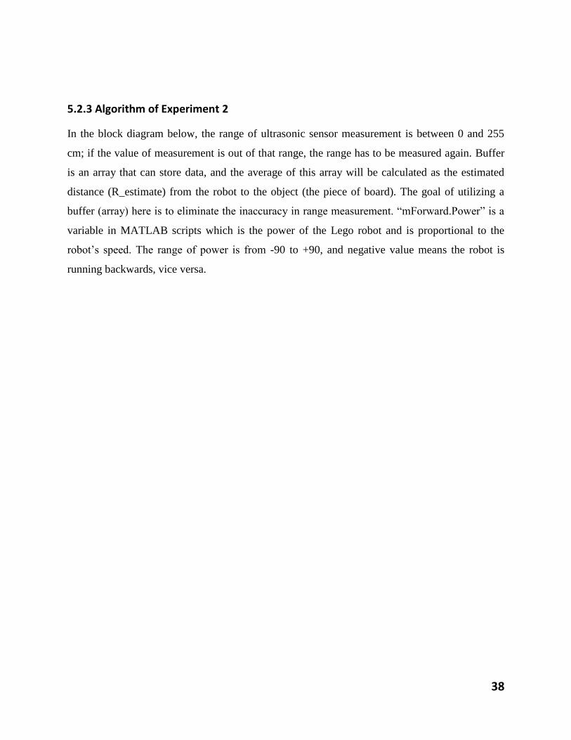
5.2.3 Algorithm of Experiment 2
In the block diagram below, the range of ultrasonic sensor measurement is between 0 and 255
cm; if the value of measurement is out of that range, the range has to be measured again. Buffer
is an array that can store data, and the average of this array will be calculated as the estimated
distance (R_estimate) from the robot to the object (the piece of board). The goal of utilizing a
buffer (array) here is to eliminate the inaccuracy in range measurement. “mForward.Power” is a
variable in MATLAB scripts which is the power of the Lego robot and is proportional to the
robot’s speed. The range of power is from -90 to +90, and negative value means the robot is
running backwards, vice versa.
39
START
Open sensor A and sensor B
Get Range A and Range B (cm)
0<=RA<=255 cm AND 0<=RB<=255 cm
Fill out the buffer A and buffer B, get average value of buffer
R_estimate A and R_estimate B
(cm)
R_estimate=(R_estimate A+R_estimate B)/
2 (cm)
R_estimate>=30 cm
Robot speed up, mForward.Power(i+1)=mForward.
Power(i)+pow (scale)
YES
NO
YES
NO
mForwad.power>=powerLimit (unit:scale)
If R_estimate<30
cm
Robot slow down, mForward.Power(i+1)=mForward.Power(i)
-pow
mForwad.power<=-powerLimit (scale)
Keep the current speed
moveing
YES
R_estimate=30cm
NO
Stop the robot
End
NO
YES NO
i=i+1
Figure 5.2.3: Block Diagram of experiment #2
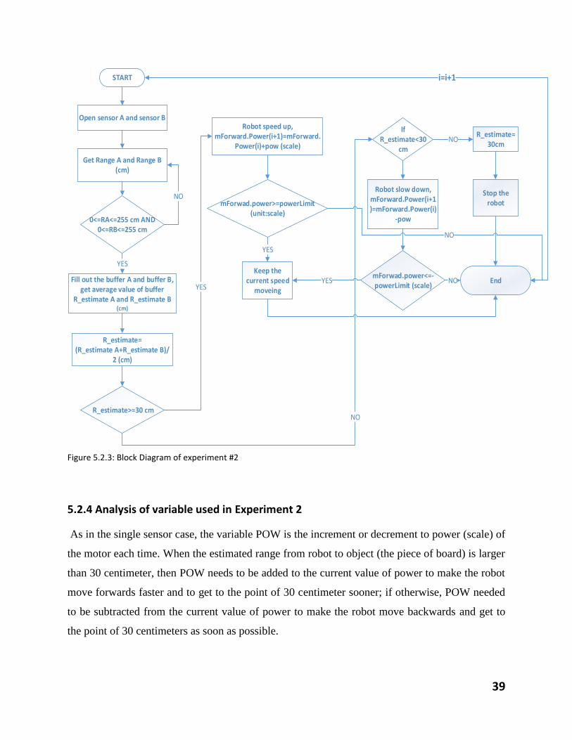
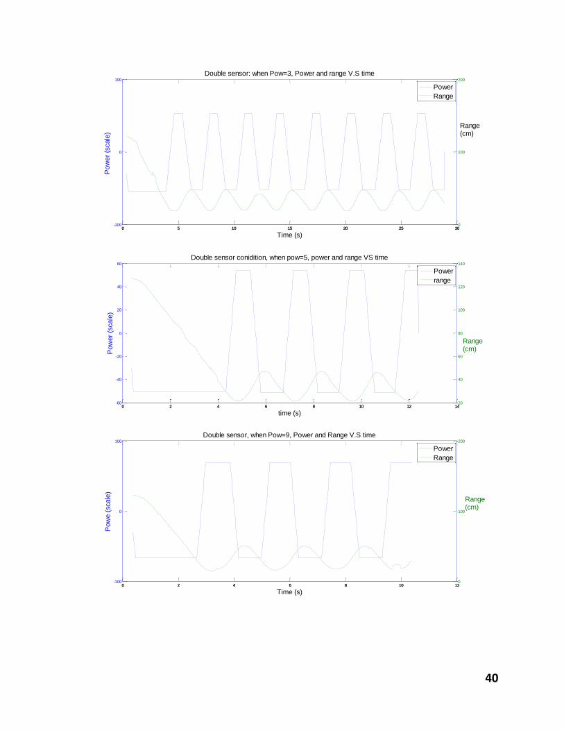
5.2.4 Analysis of variable used in Experiment 2
As in the single sensor case, the variable POW is the increment or decrement to power (scale) of
the motor each time. When the estimated range from robot to object (the piece of board) is larger
than 30 centimeter, then POW needs to be added to the current value of power to make the robot
move forwards faster and to get to the point of 30 centimeter sooner; if otherwise, POW needed
to be subtracted from the current value of power to make the robot move backwards and get to
the point of 30 centimeters as soon as possible.
40
0 5 10 15 20 25 30-100
0
100
Time (s)
Pow
er
(scale
)
Double sensor: when Pow=3, Power and range V.S time
0 5 10 15 20 25 300
100
200
Power
Range
Range(cm)
0 2 4 6 8 10 12 14-60
-40
-20
0
20
40
60
time (s)
Pow
er
(scale
)
Double sensor conidition, when pow=5, power and range VS time
0 2 4 6 8 10 12 1420
40
60
80
100
120
140
Power
range
Range(cm)
0 2 4 6 8 10 12-100
0
100
Time (s)
Pow
e (
scale
)
Double sensor, when Pow=9, Power and Range V.S time
0 2 4 6 8 10 120
100
200
Power
Range
Range(cm)
41
5.3 Experiment 3: A Lego robot exactly is following the path of the
other moving object
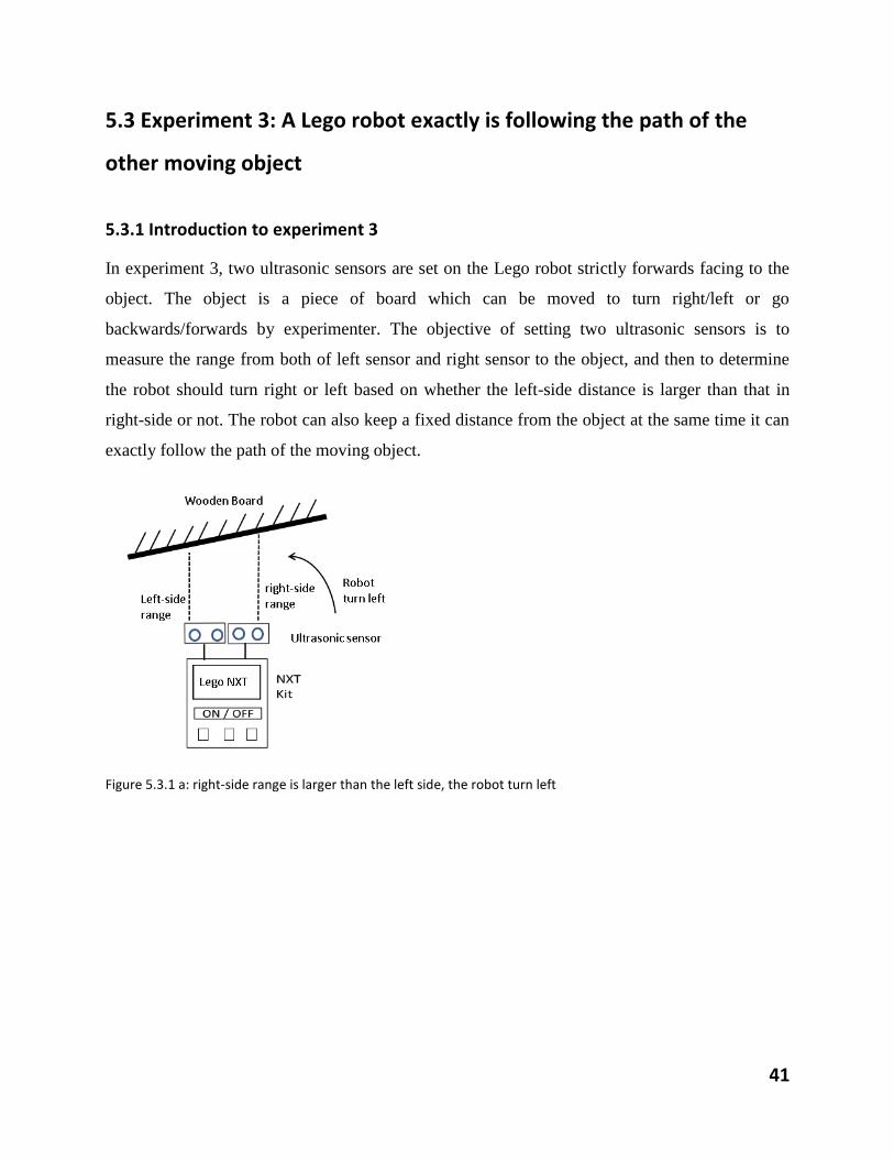
5.3.1 Introduction to experiment 3
In experiment 3, two ultrasonic sensors are set on the Lego robot strictly forwards facing to the
object. The object is a piece of board which can be moved to turn right/left or go
backwards/forwards by experimenter. The objective of setting two ultrasonic sensors is to
measure the range from both of left sensor and right sensor to the object, and then to determine
the robot should turn right or left based on whether the left-side distance is larger than that in
right-side or not. The robot can also keep a fixed distance from the object at the same time it can
exactly follow the path of the moving object.
Figure 5.3.1 a: right-side range is larger than the left side, the robot turn left
42
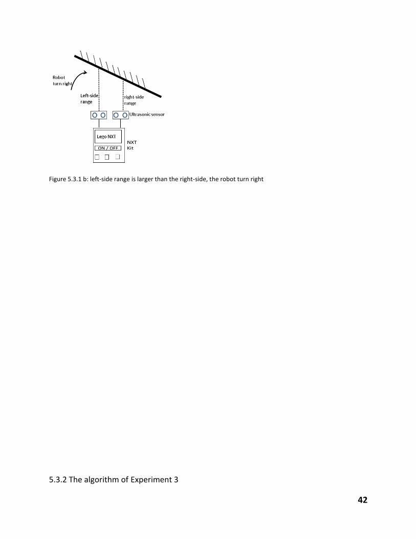
Figure 5.3.1 b: left-side range is larger than the right-side, the robot turn right
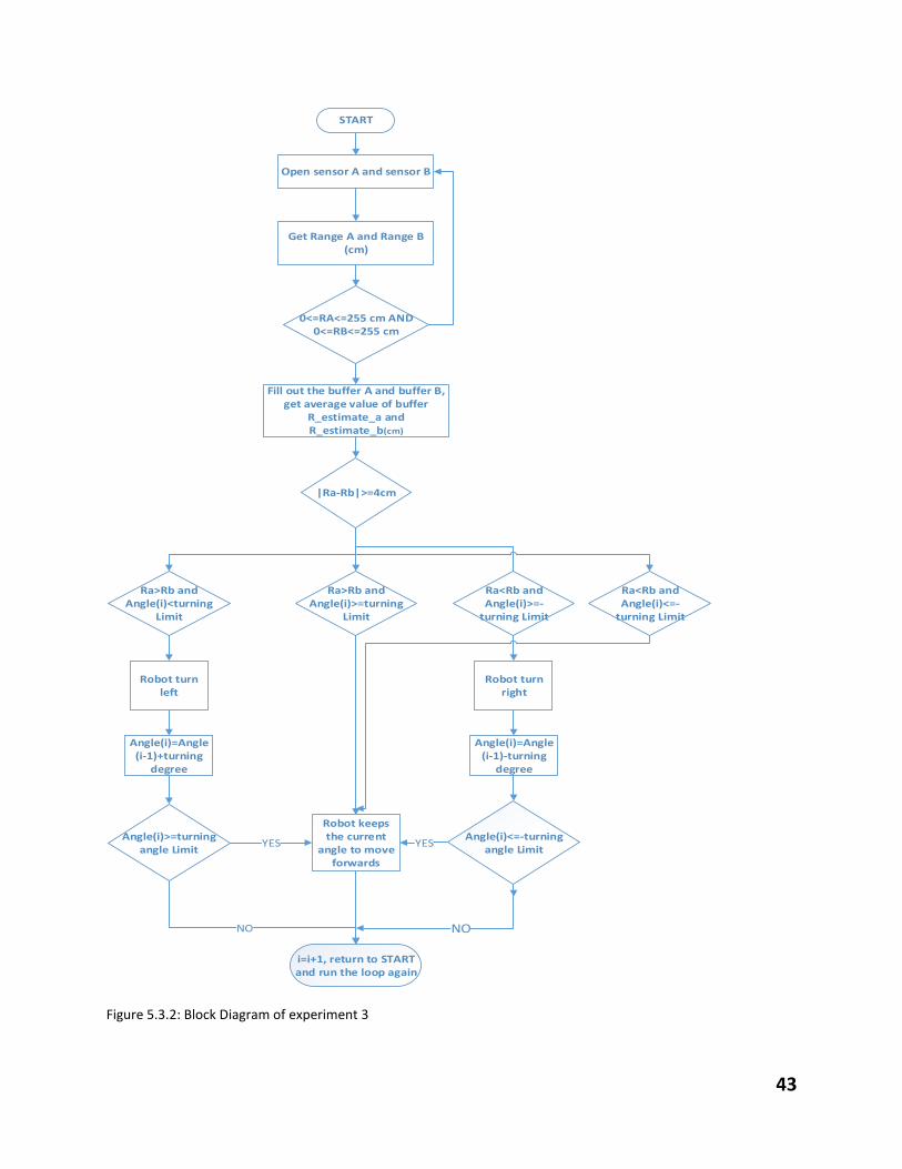
5.3.2 The algorithm of Experiment 3
43
START
Open sensor A and sensor B
Get Range A and Range B (cm)
0<=RA<=255 cm AND 0<=RB<=255 cm
Fill out the buffer A and buffer B, get average value of buffer
R_estimate_a and R_estimate_b(cm)
|Ra-Rb|>=4cm
Robot turn left
Angle(i)=Angle(i-1)+turning
degree
Angle(i)>=turning angle Limit
Robot keeps the current
angle to move forwards
Ra>Rb and Angle(i)<turning
Limit
Ra>Rb and Angle(i)>=turning
Limit
Ra<Rb and Angle(i)>=-
turning Limit
Ra<Rb and Angle(i)<=-
turning Limit
Robot turn right
Angle(i)=Angle(i-1)-turning
degree
Angle(i)<=-turning angle Limit
YES YES
i=i+1, return to START and run the loop again
NO NO
Figure 5.3.2: Block Diagram of experiment 3
44
5.3.3 Analysis of variables used in Experiment 3
In the block diagram of experiment 3, the condition when the robot should turn is that when the
difference of left-side and right-side sensor measuremnt is larger than 4 centimeters. Under this
condition, when left-side measuremnt of ultrasonic sensor is larger than the other one, the robot
should turn right (figure 5.3.1b), vice versa (figure 5.3.1a). Variable angle means how much
degrees the wheels has been turning. The variable angle has a range from negative 70 degrees to
positive 70 degrees. Since NXTMotor has a parameter called TachoLimit, which indicates the
degree the motor reasch at each time. Therefore, the value of TachoLimit is the turning degree of
the motor at each time. When the robot is turning left, the current angle is equal to sum of the
turning degree and angle of last time. When the robot is turning right, the curent angle is equal to
the value of angle in last time subtact the turning degree. From the sign of current anlge, it is
clear to know whether the robot is now turning right or left. There is a special situation needed to
be considered: when the angle has already get to its maximum value (70 degree) but the robot
still needs to turn left based on the logic in programming, then the robot will keep current
movement until the coniditon has changed. In the other situation, when the anlge has get to its
minimum value (-70 degrees) but the robot still needs to turn right, then the robot will keep the
current movement until the condition has been changed based on the measurement of distance
from both the left-side and right-side sensor to the object.
5.3.4 Constraints in Experiment 3
When connecting the Lego robot to laptop with Bluetooth, the robot performs unsteadily. For
example, MATLAB showed an error that the NXT was disconnected, though the robot has been
already connected to the PC’s Bluetooth. An alternative way is to use USB port to connect the
robot to laptop. While the normal USB port is also not long enough to connect the robot with
laptop when the robot is running, so a 5-meter USB port has been used for connection. Another
constraint is that when the NXT intelligent in a low battery mode, there were not enough current
passing through the wire which may causes the robot reacts slowly and not effectively. To make
sure the data got from the sensor is accurate, the robot should be operated when the battery level
is larger than half of the full. In addition, based on the calibration result from section 4.4, the
angle with which the piece of board is moved to right or left cannot be larger than 40 degree,
45
because the ultrasonic sensor will not measure range accurately when the turning angle of the
board is larger than 45 degrees.
5.3.5 Future progress of experiment 3
Due to the time constraints, only the left-side and right-side ranges were used to determine
whether the robot should turn left or right to follow the path of the leading object and to keep a
fixed distance from the object. If the time is permitted, the left-side echoic flow τ_L and right-
side echoic flow τ_R can be computed based on the range and change in range. Then, the next
step will be to compare the echoic flow to determine the movements of the robot.
5.3.6 Conclusion of experiment 3
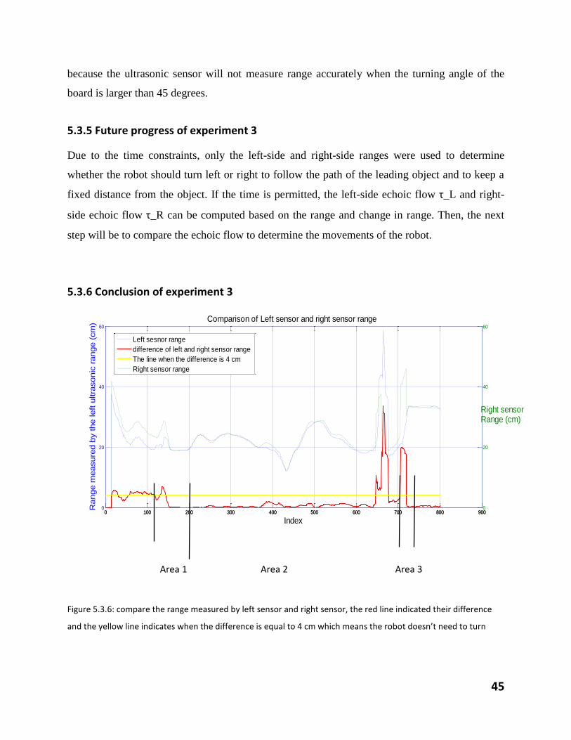
Figure 5.3.6: compare the range measured by left sensor and right sensor, the red line indicated their difference
and the yellow line indicates when the difference is equal to 4 cm which means the robot doesn’t need to turn
0 100 200 300 400 500 600 700 800 9000
20
40
60
Index
Range m
easure
d b
y the left u
ltra
sonic
range (
cm
)
Comparison of Left sensor and right sensor range
0 100 200 300 400 500 600 700 800 9000
20
40
60
Left sesnor range
difference of left and right sensor range
The line when the difference is 4 cm
Right sensor range
Right sensorRange (cm)
Area 1 Area 3 Area 2
46
Based on the graph above and the actual movement of Lego robot, the robot’s real movemnt
when following a pice of board, follows the logic in programming and its path also fits to the
graph above. For example, in area 1 (figure5.3.6), it is clear that the difference (red line) between
the range measured by left and right sensor is larger than 4 cm (yellow line), and the range
measured by right senor is larger than the range measured by the other, the robot turned left. In
area 2, since the difference of left-side and right-side measurement is smaller than 4 cm, so the
robot didn’t execute the command of turning right/left and only moved forward to follow the
object. In area 3, converse to the situation in area 1, the range measured by left sensor is much
larger than the other one, so the robot turned right.
Chapter 6: Conclusion
In this section, the conclusion of three experiments which also include the calibrated results and
the future progress of experiments will be discussed.
6.1 Overall Conclusion
By applying the background theories to properly calibrated Lego NXT, a robot can be built to
relize the goal of all three experiments.First, the robot with only one ultrasonic sensor working
can follow an moving object straightly and also can keep a fixed distance from the obejct by
measuring the range to the obejct. When two ultrasonic sensor work, the robot can still follow a
moving object straighly forwrads and backwards by using the avergae range bwtween the two
range measured by left and right ultraosnic senosr. Moreover, the Lego robot showed its ability
to exactly follow the moving obejct when the object start to turn right or left; the robot used two
ultrasonic sensors to mesure the range and compare the range difference to determine whether
turn right or left. Based on the result of these three experiments, a Lego NXT robot with
ultraosnic sensors can successfully applies the theory of echo location and echoic flow theorem
to practice when exactly follow the path of a moving obejct.
6.2 Future application of the project
The performance of the Lego roobt when applying echoic flow theorem was restricted by a large
number of factors, such as the error existing in the hardware of experimental hadware, the noise
47
signal disturbing the performance of facilities, etc. However, the alogarithm of this project can
be applied to devices which can result more accuracte measurements by using the same theorems.
For the practical application of this project, this project can be applied to automation cruise
control system. By knowing the distance between my vehicle and the front or back vehicle, the
speed of vehicle can be controlled to aviod car accidents or traffic jam. Automation cruise
control which has been installed to some of cars today has helped drivers avoid subconsciously
violating speed limits and also reduced drivers’ fatigue for logn drives.
48
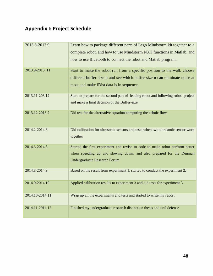
Appendix I: Project Schedule
2013.8-2013.9 Learn how to package different parts of Lego Mindstorm kit together to a
complete robot, and how to use Mindstorm NXT functions in Matlab, and
how to use Bluetooth to connect the robot and Matlab program.
2013.9-2013. 11 Start to make the robot run from a specific position to the wall; choose
different buffer-size n and see which buffer-size n can eliminate noise at
most and make fDist data is in sequence.
2013.11-203.12 Start to prepare for the second part of leading robot and following robot project
and make a final decision of the Buffer-size
2013.12-2013.2 Did test for the alternative equation computing the echoic flow
2014.2-2014.3 Did calibration for ultrasonic sensors and tests when two ultrasonic sensor work
together
2014.3-2014.5 Started the first experiment and revise to code to make robot perform better
when speeding up and slowing down, and also prepared for the Denman
Undergraduate Research Forum
2014.8-2014.9 Based on the result from experiment 1, started to conduct the experiment 2.
2014.9-2014.10 Applied calibration results to experiment 3 and did tests for experiment 3
2014.10-2014.11 Wrap up all the experiments and tests and started to write my report
2014.11-2014.12 Finished my undergraduate research distinction thesis and oral defense
49
Appendix II: Experiment 1 MATLAB code COM_CloseNXT('all') close all clear all clc
dis=30; %fixed distance pow=3; %reduced/increased power powerlimit=70; Tick=0; idTicks=1; tolerance=7; nBufferSize=14; nNumTicks=1000; %lport=SENSOR_4; rport=SENSOR_4; hNXT=COM_OpenNXT(); COM_SetDefaultNXT(hNXT); %OpenUltrasonic(lport); OpenUltrasonic(rport); Wheels=[MOTOR_B;MOTOR_C]; drivingPower=30; drivingPower1=-30; turningPower = -30; turningDist = 100;
mForward=NXTMotor(Wheels,'Power',drivingPower); mBackward=NXTMotor(Wheels,'Power',drivingPower1); mBackward.SmoothStart=true; mForward.SmoothStart=true; i=1; power(i)=drivingPower; tic fDistBuffer=zeros(1,nBufferSize); %r_fDistBuffer=zeros(1,nBufferSize); while 0<1 %idTicks<nNumTicks mForward.SendToNXT(); fDist=GetUltrasonic(SENSOR_4)-tolerance; %fDist2=GetUltrasonic(SENSOR_2)-tolerance;
fd(i)=fDist; %fd2(i)=fDist2; if fDist>=0 && fDist<=255 fDistBuffer(2:end)=fDistBuffer(1:end-1); fDistBuffer(1)=fDist;
if Tick>=nBufferSize %for i=1:nlength fRangeEstimate=mean (fDistBuffer); d(i)=fRangeEstimate; % fRangeEstimate2=mean(r_fDistBuffer); % d_r(i)=fRangeEstimate2;
50
%i=i+1; tCurrentTime=toc; t(i)=tCurrentTime; if abs(fRangeEstimate-dis)>0 % differ=abs(fRangeEstimate-dis); if fRangeEstimate<=dis fprintf('please slow down\n'); mForward.Power=power(i)-pow; power(i+1)=mForward.Power;
if mForward.Power==0 mForward.Power=mForward.Power-1; power(i+1)=mForward.Power; else if power(i+1)<=-powerlimit power(i+1)=power(i); end end %fprintf('stop'); else fprintf('please speed up\n'); differ=fRangeEstimate-dis; mForward.Power=power(i)+pow; power(i+1)=mForward.Power; if power(i+1)>=powerlimit power(i+1)=power(i); end %break; end else mForward.Power=0; power(i)=mForward.Power; mForward.Stop('off'); CloseSensor(SENSOR_1); COM_CloseNXT(hNXT); end i=i+1; end Tick=Tick+1; % idTicks=idTicks+1;
end
end
51
Appendix III: Experiment 3 MATLAB code
COM_CloseNXT('all') close all clear all clc Tick=0; idTicks=1; tolerance=3; nBufferSize=14; nNumTicks=1000; d_threshold=8;
turnlimit=60; full_l=false;full_r=false; % current degree hasn't get to turn limit currentdegree_r(1)=0;currentdegree_l(1)=0; degree(1)=0; truningdegree=0; % turning degree at first lport=SENSOR_1; rport=SENSOR_4;
hNXT=COM_OpenNXT(); COM_SetDefaultNXT(hNXT);
OpenUltrasonic(lport); OpenUltrasonic(rport); Wheels=[MOTOR_A;MOTOR_C;]; drivingPower=-30;
mForward=NXTMotor(Wheels,'Power',drivingPower); mForward.SmoothStart=true; mBackward=mForward; mBackward.Power=-drivingPower; mBackward.SmoothStart=true; TurnleftB=NXTMotor(MOTOR_B,'Power',-25); % negative driving power: turn left TurnleftB.SpeedRegulation=false; TurnleftB.TachoLimit=10; %Turnleft.ActionAtTachoLimit='Brake'; TurnleftB.SmoothStart=true; Turnright=TurnleftB; Turnright.Power=25; Turnleft_ex=TurnleftB; Turnleft_ex.TachoLimit=40; Turnright_ex=Turnright; Turnright_ex.TachoLimit=40; i=1; j=1; k1=1;k2=1;
52
l_fDistBuffer=zeros(1,nBufferSize); r_fDistBuffer=zeros(1,nBufferSize); while 0<1 TurnleftB.TachoLimit=10; Turnright.TachoLimit=10; tic mForward.SendToNXT();
fDist_l=GetUltrasonic(lport)-tolerance; fDist_r=GetUltrasonic(rport)-tolerance;
fd_l(i)=fDist_l; fd_r(i)=fDist_r;
fprintf('go'); if fd_l(i)>=0 && fd_l(i)<=255 && fd_r(i)>=0 && fd_r(i)<=255 l_fDistBuffer(2:end)=l_fDistBuffer(1:end-1); l_fDistBuffer(1)=fDist_l; r_fDistBuffer(2:end)=r_fDistBuffer(1:end-1); r_fDistBuffer(1)=fDist_r; if Tick>=nBufferSize %for i=1:nlength fRangeEstimate_l=mean (l_fDistBuffer); d_l(i)=fRangeEstimate_l; fRangeEstimate_r=mean(r_fDistBuffer); d_r(i)=fRangeEstimate_r;
if d_l(i)~=d_r(i) differ=abs(d_l(i)-d_r(i)); difference(i)=differ;
if differ>6 j=j+1; if d_r(i)>d_l(i) && full_l==false if degree(j-1)<0 TurnleftB.TachoLimit=abs(degree(j-1)); TurnleftB.SendToNXT(); TurnleftB.WaitFor(); degree(j-1)=degree(j-1)+TurnleftB.TachoLimit; end TurnleftB.TachoLimit=10; TurnleftB.SendToNXT(); TurnleftB.WaitFor();
fprintf('turnleft1:%d\n',i); degree(j)=degree(j-1)+TurnleftB.TachoLimit; currentdegree_l=[currentdegree_l,TurnleftB.TachoLimit]; degree_l=sum(currentdegree_l);
53
if degree_l>=turnlimit %TurnleftB.TachoLimit=turnlimit-sum(currentdegree_l(1:end-
1)); full_l=true;
else end % elseif d_r(i)>=d_l(i) && full_l==true pause(0.3); fprintf('keep turning left:%d\n',i); degree(j)=degree(j-1); elseif d_l(i)>d_r(i) && full_r==false if degree(j-1)>0 Turnright.TachoLimit=degree(j-1); Turnright.SendToNXT(); Turnright.WaitFor(); degree(j-1)=degree(j-1)-Turnright.TachoLimit; end Turnright.TachoLimit=10; Turnright.SendToNXT(); Turnright.WaitFor(); fprintf('turnright1:%d\n',i); currentdegree_r=[currentdegree_r,-Turnright.TachoLimit]; degree_r=sum(currentdegree_r); degree(j)=degree(j-1)-Turnright.TachoLimit; if degree(j)<=-turnlimit % Turnright.TachoLimit=sum(currentdegree_r(1:end-
1))+turnlimit; full_r=true; % degree(j)=degree(j-1); else end
elseif d_l(i)>d_r(i) && full_r==true pause(0.3); fprintf('keep right:%d\n',i); degree(j)=degree(j-1); end
else if degree(j)>0 Turnright.TachoLimit=degree(j); Turnright.SendToNXT(); Turnright.WaitFor(); fprintf('keep same'); degree(j)=0; full_l=false; full_r=false; elseif degree(j)<0 TurnleftB.TachoLimit=abs(degree(j)); TurnleftB.SendToNXT(); TurnleftB.WaitFor(); fprintf('keep same'); degree(j)=0; full_r=false;
54
full_l=false; end
end %
end
end
Tick=Tick+1; i=i+1; end end
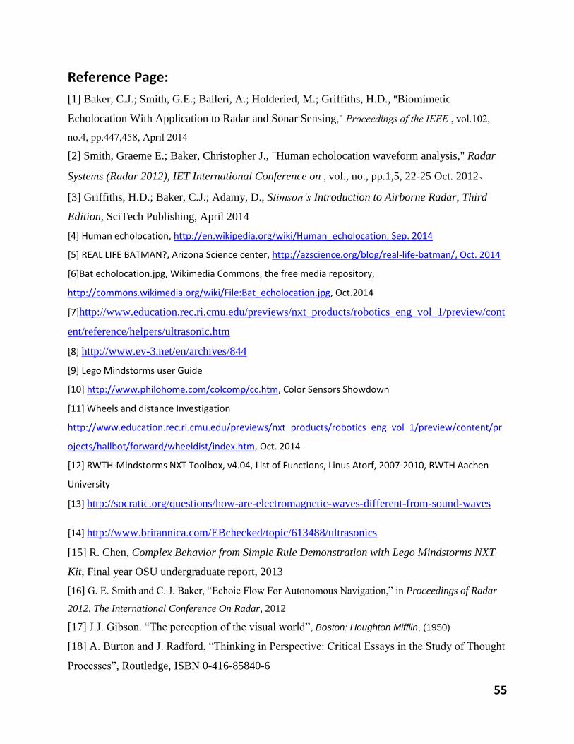
55
Reference Page:
[1] Baker, C.J.; Smith, G.E.; Balleri, A.; Holderied, M.; Griffiths, H.D., "Biomimetic
Echolocation With Application to Radar and Sonar Sensing," Proceedings of the IEEE , vol.102,
no.4, pp.447,458, April 2014
[2] Smith, Graeme E.; Baker, Christopher J., "Human echolocation waveform analysis," Radar
Systems (Radar 2012), IET International Conference on , vol., no., pp.1,5, 22-25 Oct. 2012、
[3] Griffiths, H.D.; Baker, C.J.; Adamy, D., Stimson’s Introduction to Airborne Radar, Third
Edition, SciTech Publishing, April 2014
[4] Human echolocation, http://en.wikipedia.org/wiki/Human_echolocation, Sep. 2014
[5] REAL LIFE BATMAN?, Arizona Science center, http://azscience.org/blog/real-life-batman/, Oct. 2014
[6]Bat echolocation.jpg, Wikimedia Commons, the free media repository,
http://commons.wikimedia.org/wiki/File:Bat_echolocation.jpg, Oct.2014
[7]http://www.education.rec.ri.cmu.edu/previews/nxt_products/robotics_eng_vol_1/preview/cont
ent/reference/helpers/ultrasonic.htm
[8] http://www.ev-3.net/en/archives/844
[9] Lego Mindstorms user Guide
[10] http://www.philohome.com/colcomp/cc.htm, Color Sensors Showdown
[11] Wheels and distance Investigation
http://www.education.rec.ri.cmu.edu/previews/nxt_products/robotics_eng_vol_1/preview/content/pr
ojects/hallbot/forward/wheeldist/index.htm, Oct. 2014
[12] RWTH-Mindstorms NXT Toolbox, v4.04, List of Functions, Linus Atorf, 2007-2010, RWTH Aachen
University
[13] http://socratic.org/questions/how-are-electromagnetic-waves-different-from-sound-waves
[14] http://www.britannica.com/EBchecked/topic/613488/ultrasonics
[15] R. Chen, Complex Behavior from Simple Rule Demonstration with Lego Mindstorms NXT
Kit, Final year OSU undergraduate report, 2013
[16] G. E. Smith and C. J. Baker, “Echoic Flow For Autonomous Navigation,” in Proceedings of Radar
2012, The International Conference On Radar, 2012
[17] J.J. Gibson. “The perception of the visual world”, Boston: Houghton Mifflin, (1950)
[18] A. Burton and J. Radford, “Thinking in Perspective: Critical Essays in the Study of Thought
Processes”, Routledge, ISBN 0-416-85840-6
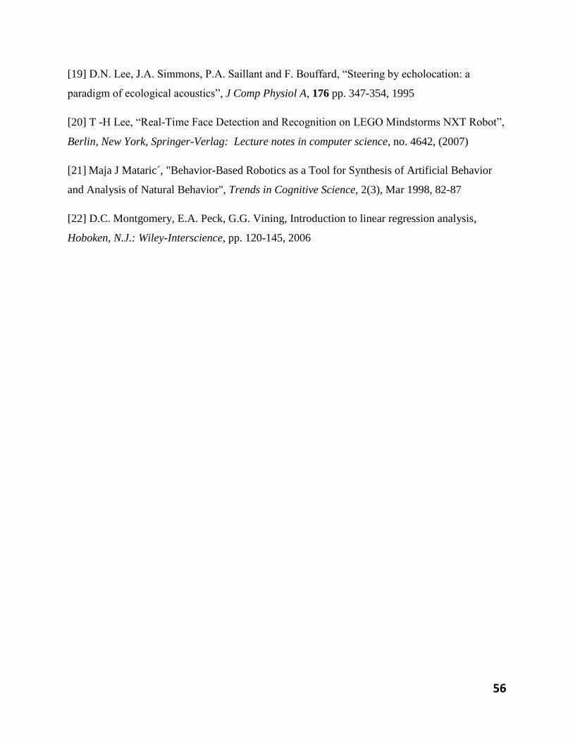
56
[19] D.N. Lee, J.A. Simmons, P.A. Saillant and F. Bouffard, “Steering by echolocation: a
paradigm of ecological acoustics”, J Comp Physiol A, 176 pp. 347-354, 1995
[20] T -H Lee, “Real-Time Face Detection and Recognition on LEGO Mindstorms NXT Robot”,
Berlin, New York, Springer-Verlag: Lecture notes in computer science, no. 4642, (2007)
[21] Maja J Mataric´, "Behavior-Based Robotics as a Tool for Synthesis of Artificial Behavior
and Analysis of Natural Behavior", Trends in Cognitive Science, 2(3), Mar 1998, 82-87
[22] D.C. Montgomery, E.A. Peck, G.G. Vining, Introduction to linear regression analysis,
Hoboken, N.J.: Wiley-Interscience, pp. 120-145, 2006