2006-1596: AN EXPERIMENT BASED STRUCTURAL DYNAMICS COURSE FORENGINEERING TECHNOLOGY STUDENTS

Jorge Tito-Izquierdo, University of Houston-DowntownJorge Tito-Izquierdo is Visiting Associate Professor of Engineering Technology. Dr.Tito-Izquierdo received his Ph.D. and M. Sc. Degrees from the University of Puerto Rico,Mayagüez, Puerto Rico, in Civil Engineering with a major in Structures. He received the CivilEngineer Degree from the Pontifical Catholic University of Peru. Dr. Tito has experience inteaching structural design, and construction management, and is a Registered ProfessionalEngineer.

Alberto Gomez-Rivas, University of Houston-DowntownAlberto Gomez-Rivas is Professor of Structural Analysis and Chair of Engineering Technology.Dr. Gomez-Rivas received Ph.D. degrees from the University of Texas, Austin, Texas, in CivilEngineering and from Rice University, Houston, Texas, in Economics. He received the IngenieroCivil degree, with Honors, from the Universidad Javeriana in Bogotá, Colombia. He also servedas Chief of Colombia’s Department of Transportation Highway Bridge Division.

Weining Feng, University of HoustonWeining Feng is Associate Professor of Process Control and Instrumentation in the EngineeringTechnology Department, University of Houston-Downtown. Dr. Feng received a Ph.D. from theDepartment of Electrical and Electronic Engineering, University of Strathclyde, Scotland, in1990. She is in charge developing UHD’s Control and Instrumentation laboratories and serves ascoordinator of the Control and Instrumentation program.

George Pincus, University of Houston-DowntownGeorge Pincus is Dean of the College of Sciences and Technology, and Professor at theUniversity of Houston-Downtown (1986-date). Prior service includes Dean of the NewarkCollege of Engineering and Professor, New Jersey Institute of Technology (1986-1994). DeanPincus received the Ph.D. degree from Cornell University and the M.B.A degree from theUniversity of Houston. Dr. Pincus has published over 40 journal articles, 2 books and is aRegistered Professional Engineer.

© American Society for Engineering Education, 2006

Page 11.187.1

AN EXPERIMENT BASED

STRUCTURAL DYNAMICS COURSE

FOR ENGINEERING TECHNOLOGY STUDENTS

Abstract

This paper describes a Structural Dynamics course for engineering technology students with

emphasis on the understanding of the theoretical concepts by using lab experiments. The

experiments involve a minimum amount of equipment.

The experiments are of increasing levels of theoretical complexity. The first two experiments

involve single degree of freedom systems. The first one is a mass-spring system with

translational motion, and the second is a rotational beam with an added mass and a spring

attached to develop an understanding of the rotational inertia and resulting natural frequency.

The third experiment consists of a simply supported aluminum beam which is used to compare

the theoretical and experimental values of the first three natural frequencies via a frequency-

domain data analysis. The fourth and fifth experiments use a simply supported reinforced

concrete beam and a simply supported prestressed concrete beam made by the students in the

Reinforced Concrete and Prestressed Concrete courses. The first natural frequencies of the

original beams were obtained experimentally and compared with the theoretical values showing

good agreement. Also, the natural frequency shows a reduction, after testing of the beams up to

the ultimate (cracked) condition. These experiments show that the first natural frequency

changes with the integrity of the beams.

The sixth experiment consisted of finding the first two natural frequencies of a steel frame

model. The properties of the frame were obtained using the geometry and results of static tests.

The frame was then dynamically excited with an electromagnetic device actuated by an

electronic signal generator. The theoretical values of natural frequencies were obtained using

structural analysis software and they showed good agreement with the experimental results.

Engineering Technology students increase their understanding of how dynamic systems perform

while also learning laboratory techniques for dynamic response testing. Verifying laboratory

obtained natural frequency against theoretically computed values provides students with robust

knowledge of dynamic system behavior.

Introduction

Structural Dynamics is an important subject for engineering technology students, because the

principles are essential for understanding different conditions such as vibration control,

earthquake and wind impact design. Structural Dynamics involves difficult theoretical and

practical concepts for a typical under-graduate engineering technology student. However, if the

course is taught using computer programs and experimental tests with data acquisition systems,

the learning curve of the main concepts of structural dynamics may be improved. This approach

is used in the Department of Engineering Technology, University of Houston – Downtown.

Page 11.187.2

The first part of the course is a brief introduction to the theory of Structural Dynamics using the

Finite Elements approach in order to obtain the matrices of mass, damping, stiffness, and forces.

The mathematics of the dynamic equations is explained but emphasis is placed on finding the

computer solution.

The computer program is explained to ensure that the students understand the input process and

the results, particularly the computation of the dynamic parameters of the structure.

In order to reinforce the theory, a series of lab experiments are designed to determine the natural

frequencies of different structures. The experimental structures are modeled using the computer

program and the predicted responses are compared to actual experimentally measured responses.

Methodology

The theory of Stiffness, Mass, Damping and Forces matrices used in the dynamic equation is

discussed following a textbook of Structural Dynamics [1]

. The stiffness matrix components of a

beam are obtained using a spreadsheet following a numerical integration method. This approach

permits the review of fundamental concepts of structural analysis, such as the relationship of

slope, deflection and acting force. The matrices are formed according to the degree of freedom

(DOF) assumed for the structure being analyzed. The commercial computer program used

handles 6 DOF per node, but the student can define fewer DOF to the desired level of

simplification.

In order to understand and verify acquired knowledge, a set of experiments are designed for this

course. The experiments are arranged in an increasing level of complexity, and basically consist

of determining the natural frequencies of the structure. The following experiments were

completed during one semester:

Experiment 1: Translational Single Degree of Freedom (SDOF)

The students construct a translational SDOF system using a tripod, a spring and a mass. A chart

will be generated which illustrates the force applied to the mass versus its deflection. The

stiffness of this system becomes the spring constant, k, which is defined as the slope of the force

vs. deflection curve.

The system vibrates after the application of a small deflection and release. The frequency of the

system is obtained visually by direct counting, which is independent of the initial deflection.

The following equation is can be used for theoretical verification:

MKf /2/1 r? (1)

where:

f = Natural frequency of the system, Hertz.

Page 11.187.3

K = Stiffness Constant of the Spring, Newton / meter

M = Mass, kilograms

The error of this experiment is close to 5%. Figure 1 shows the setup for this experiment.

Figure 1 Setup for the Translational Single Degree of Freedom System

Experiment 2: Rotational Single Degree of Freedom System

The students constructed a rotational SDOF using a tripod, a mass, and an eccentric spring with

respect to the center of gravity of the mass. The spring is the same as used in Experiment 1.

The dynamic equations are obtained from the dynamic equilibrium of the system shown in

Figures 2 and 3:

Io c%% + m(Rc%% ) R = -k.d2g

or:

(Io + mR2) c%% + k.d

2 g = 0

Where:

Spring, k

Mass, m

Page 11.187.4

c%% = Rotational acceleration of the system.

g = Rotational angle with respect to the axis of rotation.

k = Stiffness constant of a spring located at ‘d’ from the axis of rotation.

Io = Rotational Inertia of the piece of W8x13 = mass * rx2

mass = weight / g, where g is the gravity acceleration.

rx = gyration center respect to strong axis of W8x13 (from AISC manual)

m = additional mass located at a distance ‘R’ from the axis of rotation.

Defining:

M = (Io + mR2) = Equivalent mass of the system

K = k.d2

= Equivalent stiffness of the system

Then:

M c%% + Kd2g = 0 (1)

And, finally, replacing M in equation (1) the natural frequency may be obtained:

)/(2/1 2

0

2 mRIkdf -? r

The error of this experiment is close to 5%.

dk

Rotatio

n axis Io: corresponding to

a W8x13

rx = radius of gyration of W8x13Io: rx * Mass

R

c

Figure 2 Rotational Single Degree-of-Freedom System

Page 11.187.5

Figure 3: Setup for the Rotational Single Degree-of-Freedom System

Experiment 3: Simply Supported Aluminum Beam

The beam is a square tube, 1 in. by 1 in. and 0.05 in thickness. The span center-to-center of

supports is 96 in. Both supports are round bars, permitting free rotation and axial displacement

of the beam which may be modeled as a pin and roller support.

The experiment started with a static test, as shown in Figure 4, designed to obtain deflection at

the center of the aluminum beam to determine (and check) the modulus of elasticity of the

material.

The aluminum beam was then tested dynamically in order to find its first three natural

frequencies. The experimental results were compared with the mathematical model and with the

results of a finite elements analysis.

A rubber bicycle wheel was used to impact the center of the aluminum beam. An oscilloscope

was used to capture the vibration measurement signal from an accelerometer located at the one-

fourth point of the beam span. Recorded data is voltage vs. time in second. After obtaining time

domain data, Fast Fourier Transformation (FFT) analysis is used to convert the sampled data into

voltage vs. frequency [2]

, as shown in Figures 5 and 6 where the prominent peaks corresponding

to the structural frequency modes.

Only 512 readings of 1000 sampled data points acquired by the digital oscilloscope are used for

FFT to compute the natural frequency. With the accelerometer located at one-fourth of the beam

span, the experimental results for the first three natural frequencies are: 13.0 Hz, 48.0 Hz, and

112.4 Hz. This particular location of the accelerometer is selected to permit the capture of these

natural frequencies.

Page 11.187.6

The theoretical values from the closed formulation were obtained using the following equation:

f = の/(2r)

Where:

* +mIELn x /.]/)[( 222ry ?

f = Natural frequency in cycles/sec or Hz for mode n

の = Circular frequency, in rad/sec

n = Mode number

L = Beam span

E = Modulus of elasticity of aluminum

Ix = Centroidal moment of inertia of the beam respect to the horizontal axis

m = Mass per unit length of the aluminum beam

Which yields results of 12.5 Hz, 50.0 Hz, 112.4 Hz.

The computer model using Finite Element Method (FEM) found the first three natural

frequencies as 13.0 Hz, 51.9 Hz, and 164 Hz respectively

The experimental results agree with the theoretical results with a difference of 3.8%, 4.1% and

0% for the first, second and third modes using the theoretical calculation, and 0%, 8.1% and

3.2% for the same modes using FEM. Figure 7 shows the theoretical results. The advantages of

FEM computer models are that the student can visualize the vibration shape of the aluminum

beam. Furthermore, the FEM model is more realistic, permitting the modeling of the

accelerometer mass, eccentricities, etc.

Table 1 Characteristics of the Aluminum Beam

Length in. 96

Width in. 1

Thickness in. 0.052

Known Weight lbs 2.248

Experimental Vertical Displacement in. 0.146

EI = (w*L^3)/(488*d) lbs-in 284,000

I in^4 0.0296236

E = E*I/I psi 9,586,859

Page 11.187.7

Figure 4 Static Test of the Aluminum Beam

Figure 5 Aluminum beam, accelerometer and oscilloscope

-2

-1

0

1

2

-0.1 0 0.1 0.2 0.3 0.4 0.5 0.6

0

10

20

30

40

50

60

70

0 100 200 300 400 500 600

Figure 6 Aluminum beam response: Time domain vs. frequency domain

Page 11.187.8

First

Mode

using a

FEM

computer

Second

Mode

using a

FEM

computer

Third

Mode

using a

FEM

computer

Modes

calculated

using a closed formulation.

Figure 7 Theoretical results for the first three natural

frequencies of the simply supported aluminum beam

Page 11.187.9

Experiment 4: Reinforced Concrete T-beam, before cracking, after cracking, and after

epoxy repair

A Reinforced Concrete T-Beam was designed, manufactured, and tested in order to understand

its structural behavior for different levels of load. Concrete cylinders were tested on the same

day of the T-Beam test. Thus, the Modulus of Elasticity and the concrete strength were well

defined. The steel used was a #7 rebar. The T-beam was constructed as an assignment in the

Reinforced Concrete class, but was tested during the semester by the students taking the

Dynamics of Structures course. Figures 8 and 9 show the construction process and the geometry

of the T-Beam.

The simply supported reinforced concrete T-Beam was tested dynamically to find the natural

frequency when it was sound, that is, without cracks, obtaining a natural frequency of 52 Hz.

After this test, the T-Beam was tested under a monotonic and static loading until the T-Beam

showed plastic behavior, resulting in flexure cracks in the bottom of the beam and diagonal

cracks in its web. After the T-Beam cracked, as shown in Figure 10, the natural frequency was

obtained again, as 41 Hz, showing a variation of approximately 20% less than the frequency of

the original uncracked beam. The test setup including the accelerometer and oscilloscope is

shown in Figure 11. A typical curve of acceleration versus time and the corresponding

frequency domain response is shown in Figure 12.

This T-beam was repaired after one year of the original tests. The repairing work consisted of

sealing the larger cracks with epoxy injected under pressure. The thin cracks are not repaired

because the equipment does not allow further repair. After crack sealing, the natural frequency

is again obtained, showing the same value as those from the sound beam. This shows that small

cracks do not change the natural frequency of the beam, only thick and large cracks are

important.

Figure 8 Construction of the Reinforced Concrete T-Beam

Page 11.187.10

Figure 10 Setup of the static test and cracks of the Reinforced Concrete T-beam

12"

3"

1"

2" 0.75"

1"

1" 8"

1 # 7

Span support-to-support: 9’6”

Figure 9 Geometry of Reinforced Concrete T-Beam

Page 11.187.11

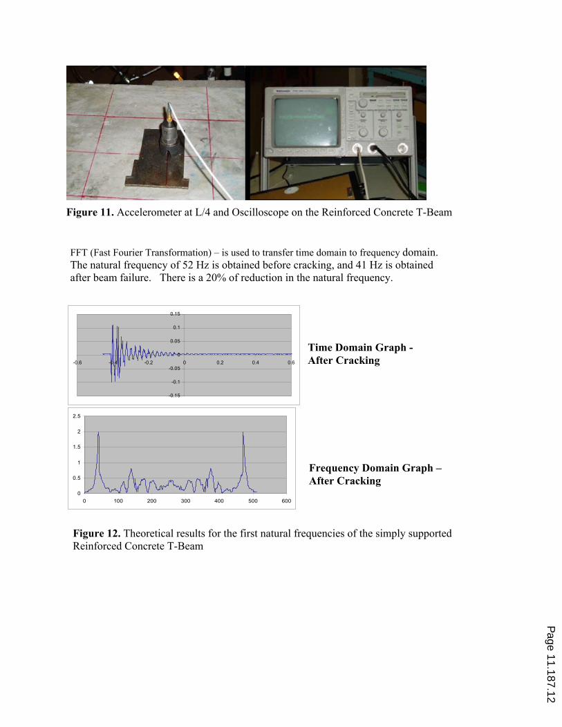
Figure 11. Accelerometer at L/4 and Oscilloscope on the Reinforced Concrete T-Beam

FFT (Fast Fourier Transformation) – is used to transfer time domain to frequency domain.

The natural frequency of 52 Hz is obtained before cracking, and 41 Hz is obtained

after beam failure. There is a 20% of reduction in the natural frequency.

0

0.5

1

1.5

2

2.5

0 100 200 300 400 500 600

-0.15

-0.1

-0.05

0

0.05

0.1

0.15

-0.6 -0.4 -0.2 0 0.2 0.4 0.6

Time Domain Graph -

After Cracking

Frequency Domain Graph –

After Cracking

Figure 12. Theoretical results for the first natural frequencies of the simply supported

Reinforced Concrete T-Beam

Page 11.187.12

Experiment 5: Post-Tensioned Concrete T-Beam before, after cracking, and after crack

sealing.

The Post-tensioned Concrete T-beam was constructed as part of the objectives of the

Prestensioned Concrete Design class, but was tested by the students taking the Structural

Dynamics course. The T-Beam was designed, manufactured, and tested in order to understand

its structural behavior for different levels of load. The concrete used was characterized using

cylinders which were tested on the same day of the T-Beam test, in this way the Modulus of

Elasticity and the Strength of the concrete were well defined. The high strength steel is a 3/8”

strand. Figure 13 shows the geometry of the T-Beam.

The T-Beam was tested dynamically to find the natural frequency when it was sound, or without

cracks, obtaining a natural frequency of 35 Hz. After this test the T-Beam was tested under a

monotonic and static loading until the T-Beam showed its plastic behavior, resulting in flexure

cracks in the bottom of the beam, as shown in Figure 14. The natural frequency of the cracked T-

Beam was measured to be 29 Hz, showing a variation of approximately 20% less than the

frequency corresponding to a sound beam. The setup of the accelerometer and oscilloscope is

similar to that of Figure 10.

This T-beam was repaired after 6 months of the original tests. The repairing work consists in

sealing the thick cracks with epoxy injected under pressure. The thin cracks are not repaired

because the equipment does not allow sealing of thin cracks. After crack sealing, the natural

frequency was obtained, showing the same value as the frequency of the sound beam. This

shows that small cracks do not change the natural frequency of the beam, only thick and large

crack are significant.

3” 3”11’6”

4.1”

12”

1”

3”

8”

2-w4.5 top & bottom

Stirrup W4.5 @ 6”

3/8” A416-gr270-7wires

Figure 13. Geometry of Post-Tensioned Concrete T-Beam

Page 11.187.13

Figure 14. Setup of the static test and cracks of the Post-Tensioned Concrete T-beam

Experiment 6: One Bay – Two Stories Steel Frame

A steel frame model was constructed using 2 in x 0.125 in steel plates. The frame bay has

approximately 24 in span, and consists of 2 stories of 12 inches in height.

The first task for the students is the measurement of the real dimension of the cross-sections,

bays and heights in order to model the frame using commercial computer software.

Static horizontal loads are applied to the frame using a pulley system, as shown in Figure 15.

The horizontal displacements at each story are measured using digital dial gauges, and the strain

at the base of the column is measured using a strain gage and a strain indicator. These values are

compared with the computer program result, shown at Figure 16, obtaining the real modulus of

elasticity of the material, which is 29,900 ksi, and this value is used for the dynamic analysis.

Page 11.187.14

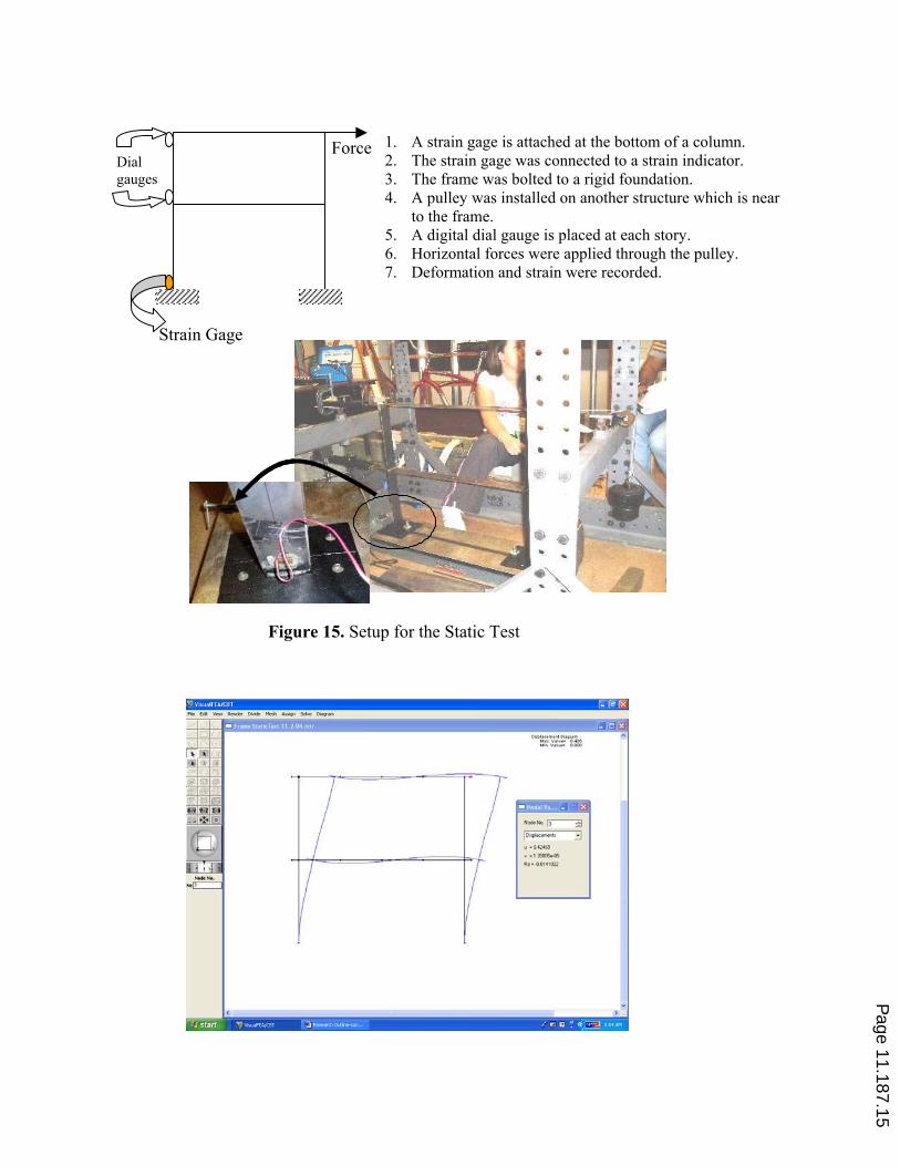
Force

Strain Gage

Dial

gauges

1. A strain gage is attached at the bottom of a column.

2. The strain gage was connected to a strain indicator.

3. The frame was bolted to a rigid foundation.

4. A pulley was installed on another structure which is near

to the frame.

5. A digital dial gauge is placed at each story.

6. Horizontal forces were applied through the pulley.

7. Deformation and strain were recorded.

Figure 15. Setup for the Static Test

Page 11.187.15

Figure 16. Displacement of the beam from the Finite Element program

Two different tests are performed on the same frame. The first test is for the frame only, without

any additional mass, and the second test consists of the frame with additional masses in the

middle of the beams.

The frequencies of the frames are obtained using three experimental methods. The first one

consists of using data from an accelerometer located at the second story, and the second method

consists of using data obtained from the strain gage located at the column base. Figure 17 shows

the setup for these methods. The frame is initially excited with a tap using a rubber hammer, and

the data (voltage versus time) from the accelerometer or strain gage is recorded in the computer.

A Fast Fourier Transformation (FFT) program is used to find the natural frequencies.

The third method consists of application of a dynamic force using an electronic function

generator that sends sinewave to a coil carefully placed near to the frame, generating an

electromagnetic force to the top of the steel frame. The frequency is varied and resonance of the

frame occurs when the excitation frequency is equal to the natural frequency. This non-

destructive method has the advantage that it may be repeated easily. Figure 18 shows the setup

for this method.

The theoretical results are obtained using the computer program Visual Analysis v5.5. The

theoretical mode shapes and frequencies are shown in Figure 19. They are obtained by modeling

the frame with the real dimensions of the model, and considering the mass of the accelerometer

only or from the masses added to the stories.

Table 2 shows that the theoretical and experimental results for the frame without additional

masses are in very good agreement; the difference is less than 3%. When additional masses are

considered, the theoretical and experimental values diverge by 17% and this may be due to the

difficulty in modeling the effect of the added masses on the rigidity and total mass of the

structure, and also may be due to rocking of the additional masses. However, the difference in

the second mode is smaller.

Figure 17. Setup for the Dynamic Test Using an Initial Excitation

Strain Gage

Accelerometer

1. The frame is bolted to the rigid foundation.

2. An accelerometer is placed on the column.

3. Oscilloscope is connected to the

accelerometer through a wire.

4. A rubber hammer is used to impact the frame.

5. The vibration data is recorded.

6. FFT is used to find the natural frequencies.

Page 11.187.16

Figure 20 Frame with Additional Masses on Beams

Dynamic

Force

Figure 18. Setup for the Dynamic Test Using a Dynamic Force

1. The frame is bolted to the rigid foundation.

2. A solenoid is closely secured to the frame.

3. A function generator is connected to the

solenoid.

4. Frequency is changed until resonance is

observed.

Figure 19. Theoretical Natural Frequencies Using the Computer Program

VisualAnalysis v5.5

Page 11.187.17

Table 2 Theoretical and Experimental Results

Test Method Natural frequency

Mode 1 (Hz)

Natural frequency

Mode 2 (Hz)

Accelerometer 8.8 32.2

Strain Gage 8.5 31.3

Dynamic Force Inducing

Resonance

8.5 --

Self Weight

only

Theoretical from

Visual Analysis v5.5

8.5 31.3

Accelerometer 6.8 22.5

Strain Gage 6.8 22.5

Dynamic Force Inducing

Resonance

6.8 --

Adding a weight

of 3.299 lb at

2nd

story, and

3.054 lb at 1st

story

Theoretical from

Visual Analysis v5.5

5.8 21.7

Conclusions

A Structural Dynamics course for undergraduate engineering technology students was developed

using the basic theory of natural frequencies and a set of experimental exercises in order to

permit the students to easily assimilate the theoretical concepts.

These experiments range from the basic one degree-of-freedom system to more complicated

experiments using beams and frames. Test specimens constructed in other courses, such as the

Reinforced Concrete and the Postensioned Concrete T-Beams were used also to demonstrate that

the theory works for real structures.

The professor can develop different methods and experiments to teach this course. It is

important the use of a Finite Elements Computer program to compare partial results and reach

conclusions about the effectiveness of the experiment.

Reference:

[1]. Tedesco, J. W., McDougal, W. G., and Ross, C. A. Structural Dynamics: Theory and Applications. Addison

Wesley Longman, Inc., 1999.

Page 11.187.18

[2] Feng, W., Gomez-Rivas, A., and Pincus, G., “An Experimental Approach for Evaluating Harmonic Frequencies

of a Flexible Beam”, ASEE 2005, Portland, Oregon.

Acknowledgement

The authors acknowledge the support from Scholars Academy of the University of Houston

Downtown for supporting students participating in this project.

Page 11.187.19