University of New MexicoUNM Digital Repository

Nuclear Engineering ETDs Engineering ETDs

Winter 1-28-2019

An Experimental and Numerical Investigation ofFlow Accelerated FLiBe CorrosionDavid B. WeitzelUniversity of New Mexico

Follow this and additional works at: https://digitalrepository.unm.edu/ne_etds

Part of the Nuclear Engineering Commons, Other Chemistry Commons, Structural MaterialsCommons, and the Transport Phenomena Commons

This Thesis is brought to you for free and open access by the Engineering ETDs at UNM Digital Repository. It has been accepted for inclusion inNuclear Engineering ETDs by an authorized administrator of UNM Digital Repository. For more information, please contact amywinter@unm.edu.

Recommended CitationWeitzel, David B.. "An Experimental and Numerical Investigation of Flow Accelerated FLiBe Corrosion." (2019).https://digitalrepository.unm.edu/ne_etds/82

i

David Weitzel Candidate

Nuclear Engineering

Department

This thesis is approved, and it is acceptable in quality and form for publication:

Approved by the Thesis Committee:

Youho Lee, Chairperson

Anil Prinja

Amir Ali

ii

AN EXPERIMENTAL AND NUMERICAL INVESTIGATION

OF FLOW ACCELERATED FLIBE CORROSION

by

DAVID WEITZEL

BACHELOR OF SCIENCE IN NUCLEAR ENGINEERING

UNIVERSITY OF NEW MEXICO, 2017

THESIS

Submitted in Partial Fulfillment of the

Requirements for the Degree of

Master of Science

Nuclear Engineering

The University of New Mexico

Albuquerque, New Mexico

May, 2019

iii

ACKNOWLEGEMENTS

I would like to acknowledge Dr. Youho Lee for his guidance and direction over

the course of our time together. He taught me that no matter how great the work you do is

if you can’t communicate it to others it profits you little.

I would like to also acknowledge Dr. Amir Ali for his help throughout my work

on the flowing FLiBe corrosion project.

I also acknowledge Dr. Anil Prinja for serving on my defense committee.

Lastly, I acknowledge the Department of Energy’s NEUP program for funding the

research in this thesis.

Thank you, Mom and Dad, your support has made everything possible.

iv

AN EXPERIMENTAL AND NUMERICAL INVESTIGATION OF FLOW

ACCELERATED FLIBE CORROSION

By

David Weitzel

B.S. Nuclear Engineering, University of New Mexico, 2017

M.S. Nuclear Engineering, University of New Mexico, 2019

ABSTRACT

Renewed interest in molten salt reactor technology has brought to light the need

for a better understanding of FLiBe corrosion. To this end a flowing FLiBe corrosion test

loop was designed to test the flow effects of FLiBe corrosion. The loop consists of a

pump, melt tank, and stainless-steel tubing assembly that heats the molten salt to high

temperatures and circulates it over test specimens. The experiment has been constructed

and has completed initial shakedown testing.

To support the flowing FLiBe experiment, a numerical corrosion model that

couples FLiBe electrochemistry, solid metal diffusion, and mass transport was

implemented. The model has been successfully validated, and initial results indicate that

the addition of nickel protective layers to structural metal will greatly reduce FLiBe

corrosion.

v

TABLE OF CONTENTS

LIST OF FIGURES ........................................................................................................ vii

LIST OF TABLES .............................................................................................................x

CHAPTER 1 INTRODUCTION ......................................................................................1

Background ..........................................................................................................................1

Material Compatibility Issues of Molten Salt reactors ............................................1

Research Objectives and Scope ...............................................................................2

The History of Molten Salt Reactor Coolants ......................................................................3

Oak Ridge Molten Salt Reactor Program ................................................................3

Post MSRE Program Research ................................................................................5

Modern MSR Designs ..............................................................................................6

CHAPTER 2 PRINCIPLES OF FLIBE CORROSION .................................................8

Physical Properties of FLiBe ...............................................................................................8

FLiBe Corrosion ................................................................................................................10

Quantitative Description of FLiBe Corrosion ........................................................10

Qualitative Description of FLiBe Corrosion ..........................................................15

CHAPTER 3 EXPERMIENT LOOP DESIGN AND CONSTRUCTION .................17

Experiment Overview and Requirements ..........................................................................17

Loop Engineering Design ..................................................................................................17

Loop Dimensions Selection ...................................................................................18

Loop Component Description ................................................................................23

Loop Construction .............................................................................................................39

Loop Shakedown Testing ...................................................................................................42

vi

Water Shakedown Test ..........................................................................................42

Molten Salt Shakedown Test .................................................................................45

CHAPTER 4 FLOWING FLIBE CORROSION MODEL .........................................53

Current Models and Their Limits.......................................................................................53

Model Implementation .......................................................................................................55

Overview ................................................................................................................55

Alloy Element Diffusion in the Solid Alloy ..........................................................56

Surface Reaction Model .........................................................................................60

Flowing Fluid Mass Transport ...............................................................................62

Model Coupling and Implementation ....................................................................63

Code Verification ...................................................................................................66

Model Validation ...................................................................................................72

Model Applications to the FHR System ............................................................................75

Bimetallic vs Single Alloy Materials .....................................................................75

Bimetallic Alloy Performance Impact on FHR Heat Exchanger Tubes ................77

Conclusion .........................................................................................................................80

REFERENCES .................................................................................................................81

vii

LIST OF FIGURES

Figure 1-1 Aircraft Reactor Experiment ..............................................................................3

Figure 1-2 Molten Salt Reactor Experiment at Oak Ridge ..................................................4

Figure 1-3 FHR Reactor Diagram ........................................................................................7

Figure 2-1 Temperature Dependent Gibbs Free Energy of Select Metal Fluorides ..........12

Figure 2-2 a: Pre-corrosion stainless steel b: Post-corrosion steel with preferential grain

boundary corrosion .................................................................................................15

Figure 3-1 Design Process Flow Chart ..............................................................................18

Figure 3-2 Relationship between fluid velocity and pipe diameter at constant Re ...........19

Figure 3-3 Constant Volume Pipe Length ........................................................................20

Figure 3-4 Diameter dependent pumping power at various Reynolds numbers ...............22

Figure 3-5 Diameter dependent starting pumping power at various Reynolds numbers ...22

Figure 3-6 Flowing FLiBe corrosion experiment loop ......................................................23

Figure 3-7 Omega FTB-1400 flow meter with signal conditioner.....................................25

Figure 3-8 Expansion Tank ................................................................................................27

Figure 3-9 Ported Expansion Tank Lid ..............................................................................27

Figure 3-10 Pyro-Tex Expansion Tank Gasket ..................................................................28

Figure 3-11 Pump and Melt Tank ......................................................................................29

Figure 3-12 Melt Tank Lid Port Layout .............................................................................30

Figure 3-13 ¼” Diameter Omegaclad K-type thermocouple .............................................31

Figure 3-14 Loop of Assembled Tubing and Fittings ........................................................34

Figure 3-15 Sample holder with samples ...........................................................................36

Figure 3-16 CFD model of sample holder ........................................................................37

viii

Figure 3-17 Glovebox Model .............................................................................................38

Figure 3-18 FLiBe loop and component pictures .............................................................39

Figure 3-19 LabVIEW software .........................................................................................40

Figure 3-20 Fully Assembled Glovebox ............................................................................41

Figure 3-21 Test loop in salt shakedown configuration .....................................................42

Figure 3-22 Frequency Dependent Pumping Power ..........................................................45

Figure 3-23 HITEC salt ......................................................................................................46

Figure 3-24 Post test sample next to unused sample .........................................................48

Figure 3-25 Post salt shakedown test loop .........................................................................49

Figure 3-26 Salt leakage around expansion tank gasket ....................................................50

Figure 3-27 Post test expansion tank interior and gasket ...................................................50

Figure 3-28 Pump outlet loop leg salt leak site ..................................................................51

Figure 2-29 Melt tank leak .................................................................................................52

Figure 4-1 Finite Difference Method Validation ..............................................................60

Figure 4-2 Mass Loss Rate for Diffusion Limited Verification Case ...............................67

Figure 4-3 Cr Concentrations for the Diffusion Limited Case .........................................68

Figure 4-4 Mass Loss Rate for Reaction Rate Limited Verification Case ........................69

Figure 4-5 Cr Concentrations for the Reaction Rate Limited Case ..................................70

Figure 4-6 Mass Loss Rate for Transport Limited Verification Case ...............................71

Figure 4-7 Cr Concentrations for Mass Transport Limited Case ......................................72

Figure 4-8 Model Calculated Mass Loss vs Validation Case Values ...............................74

Figure 4-9 Mass Loss Rate for Bimetallic Alloy of Varying Ni Thickness ......................76

Figure 4-10 Cr Concentration in Bimetallic Alloy (5 μm Ni)............................................76

ix

Figure 4-11 Mass Loss Rate FHR Heat Exchanger Tubing ..............................................78

Figure 4-12 Mass Loss for FHR Heat Exchanger Tubing ................................................79

x

LIST OF TABLES

Table 2-1 FLiBe Isotope Neutron Capture Cross Sections ..................................................8

Table 2-2 Thermophysical Properties of FLiBe .................................................................10

Table 3-1 FLiBe Loop Specifications ................................................................................24

Table 3-2 List of Swagelok Fittings ...................................................................................33

Table 3-3 Pump Calibration Results ..................................................................................44

Table 3-4 Salt shakedown sample changes ........................................................................47

Table 4-1 Finite Difference Method Node Equations ........................................................59

Table 4-2 Model Coupling Algorithm ...............................................................................65

Table 4-3 List of Constants ................................................................................................66

Table 4-4 Validation Case Values .....................................................................................73

Table 4-5 FHR Heat Exchanger Parameters ......................................................................78

1

Chapter 1: Introduction

1. Background

A. Material Compatibility Issues of Molten Salt Reactors

In recent years there has been renewed interest in molten salt reactors (MSR).

MSRs differ from conventional light water reactors in that they use molten salts as the

primary coolant instead of water. The primary reason for choosing a molten salt as the

primary coolant is to increase the reactor operating temperature which in turn increases

the plant’s thermodynamic efficiency. Li2BeF4 (FLiBe), one proposed coolant salt, is

chemically stable at high enough temperatures to be used with a combined Brayton-

Rankine power conversion cycle. MSR designs that use high temperature fluoride salts

and a pebble fuel form are referred to as Fluoride Salt Hight Temperature Reactors

(FHRs). Combined cycle power conversion is notable for having conversion efficiencies

as high as 60% compared to the 30-40% typical to a conventional Rankine cycle. This

power conversion cycle is used by the current fleet of natural gas plants which are nuclear

power’s current main market competitor. Using this more efficient power conversion

system would allow FHRs to be more market competitive.[1]

Another advantage of a molten salt coolant is that it operates at atmospheric

pressure. Existing light water reactors operated at high pressure which in turn increase the

cost of structural materials. High pressures also result in violent coolant venting when a

breach occurs. On the other hand, a molten salt system operating at atmospheric pressure

would have much lower structural strength requirements. All together this means that an

FHR would be cheaper to construct than a comparable light water reactor.[1]

2

The primary drawback to molten salt coolants is the material compatibility issues

that arise. Molten salts dissolve alloying elements out of structural materials weakening

them. Unlike typical metal corrosion, a protective oxide layer doesn’t form during molten

salt corrosion. This in turn leads to more aggressive metal corrosion.[2] Molten salt

corrosion is affected by a number of different factors including salt temperature, salt

temperature gradients, salt chemistry, fluid flow, alloy composition, and alloy

microstructure. In order to effectively predict corrosion rates and design an FHR system

these assorted factors must be understood and contextualized.

B. Research Objectives and Scope

The objective of the research presented in this thesis is to characterize the effects

of FLiBe flow on metal corrosion. Another objective is to demonstrate the corrosion

resistance of a proposed bimetallic composite consisting of Nickel-201 and Incoloy 800H.

Nickel is known to be resistant to fluoride salt corrosion, thus it is used as a protective

layer against FLiBe.[2] A better understanding of flow accelerated FLiBe corrosion is

needed to demonstrate the benefits of the composite design. To these ends a flowing

FLiBe corrosion loop was designed and constructed to investigate flow accelerated FLiBe

corrosion. In addition, a numerical model of flowing FLiBe corrosion was developed to

predict the experimental results and construct the theoretical relationship between the

various parameters of FLiBe corrosion.

The scope of the research is as follows. The flowing FLiBe corrosion experiment

is conducted over the temperature range of 600 to 700 C and under laminar flow

conditions. The entirety of the test loop was designed, procured and built during the

course of this research. Fabrication of the bimetallic alloy was handled by a research

3

collaborator. Lastly the numerical model of flow accelerated FLiBe corrosion was

researched and developed to support the above-mentioned experimental work.

2. The History of Molten Salt Reactor Coolants

A. Oak Ridge Molten Salt Reactor Program

MSR technology had its birth with the aircraft reactor program that started in

1950. At the time the US Air Force was interested in a nuclear-powered aircraft for long

range, long endurance bombing missions against strategic targets in the USSR. The initial

salt and material selections for molten salt reactors was done over the course of the

program. In 1953 the Aircraft Reactor Experiment (see figure 1-1), a small molten salt

reactor, was brought online and ran for several days.[3] The program officially ended in

1956 as interest in an aircraft reactor dropped off due to the development of

intercontinental ballistic missiles and long-range jet bombers.

Figure 1-1 Aircraft Reactor Experiment[2]

4

While on paper the Aircraft Reactor Program ended in 1956, in reality the project

team transitioned into commercial reactor development. One of the major changes that

occurred early during the civilian reactor program was the introduction of fuel breeding as

a design focus in 1959.[3] At the time a major industry concern was the depletion of world

uranium resources. At the time breeder reactors were the focus of the Atomic Energy

Commission (AEC) and the MSR program was adjusted to accommodate this focus. The

Molten Salt Reactor Experiment (MSRE) was proposed to the AEC at the end of 1959.

The proposal was accepted, and design work started during the summer of 1960. The

reactor consisted of a 1.37 m diameter and 1.62 m high graphite core with a liquid fuel

salt. In 1962 construction started, and in 1965 the reactor went critical.[3] Figure 1-2

shows a photograph of the MSRE reactor core.

Figure 1-2 Molten Salt Reactor Experiment at Oak Ridge[2]

5

After a thorough shakedown process, reliable continuous operation was achieved in late

1966. From December 1966 through March 1968 the MSRE operated most of the time

conducting various experiments. The reactor fuel was then changed from U-235 to U-233

and ran again from January through May 1969. The MSRE was the first reactor to ever

run with U-233. The experiment continued through the end of 1969 and was then ended

to transfer funding to other areas within the MSR program. The MSRE experiment

produced an invaluable amount of operational data for MSRs and over the course of the

experiment many instrumental technologies such as online melt chemistry control, needed

for a power reactor were developed. Political support for the MSR program however

began to dry up in the seventies which culminated in the cancelation of the program in

1976.[3]

B. Post MSRE Program Research

After the US MSR program was shut down MSR research became sporadic with

some industry research and international research in places such as Japan.[3] Fluoride salt

research lived on as a prospective fusion reactor breeder blanket.[4] Recent research has

primarily taken the form of small scale static material exposure tests and other university

lab scale experiments. The fortunes of MSR research however began to change with the

generation IV reactor initiative. The new push in MSR technology has been characterized

by new design efforts at leading universities as well as the development of new FLiBe

purification and testing facilities.[2] A number of new startup companies have started to

develop commercial MSR reactors.

6

C. Modern MSR Designs

One of the leading modern MSR designs is the FHR mentioned earlier in this

chapter. The Fluoride Salt High Temperature Reactor (FHR) concept was developed by

the University of California, Berkeley, the Massachusetts Institute of Technology, and the

University of Wisconsin.[1] The design goals were to address the economic, licensing, and

design challenges facing modern MSRs. The key design characteristics of the reactor are

as follows.

The FHR is a 236 MWth small modular reactor will pebble fuel form and molten

FLiBe as the primary coolant. The FHR was designed to be compatible with existing air-

Brayton combined cycle systems used in natural gas plants. The plant is expected to

produce 100 MWe when coupled to such an air-Brayton power conversion system. The

fuel pebbles are 3.0 cm in diameter and consist of TRISO fuel particles in a graphite

matrix. Each pebble contains 1.5 g of uranium fuel. Fuel pebbles are expected to be

depleted over 1.4 years and due to the pebble bed design can be continuously replaced.

The FLiBe coolant will flow upward through the core with the fuel pebbles floating up

with the coolant. The outer pebbles will be inert reflector pebbles. The reactor vessel is

3.5 meters in diameter and 12 meters tall and consists of a graphite reflector and fuel

channel for the pebbles. The graphite in the core is the primary tritium sink in the reactor.

The FLiBe heated in the core the flows through coiled tube air heaters to transfer the

energy into the combined air-Brayton cycle. Figure 1-3 shows a diagram of the FHR

reactor core. All together the FHR as described above integrates a number of recent

innovations with preexisting MSR technology.[1]

7

Figure 1-3 FHR Reactor Diagram[1]

One area of lingering concern for the FHR is the issue of structural metal

corrosion in FLiBe. While existing research from the MSRE program suggest that

corrosion will be within acceptable limits, a better mechanistic understanding of FLiBe

corrosion is needed for a more precise material selection and design.

8

Chapter 2: Principles of FLiBe Corrosion

1. Physical Properties of FLiBe

FLiBe is a eutectic salt mix of 66% LiF and 33% BeF2. The term FLiBe comes

from rearranging the constituent elemental symbols of the salt into an easy to use

monosyllable form. FLiBe salt was chosen as a reactor coolant for a number of

overlapping reasons including its low impact on neutronics, low viscosity, and low

melting point compared to other molten salts.[2] The reason for these advantages comes

from the nature of the elements in question.

FLiBe is an excellent material in terms of neutronics. Each of the constituent

isotopes with the exception of Li6 have low neutron capture cross sections. Table 2-1 lists

the neutron capture cross sections of each of the naturally occurring constituents of

FLiBe.

Table 2-1 FLiBe Isotope Neutron Capture Cross Sections

Isotope Neutron Capture Cross Section

Be9 8 mb[5]

F19 9.5 mb[5]

Li7 45 mb[5]

Li6 941 b (n,α)[5]

Lithium 6 has a large cross section of 941 b for its neutron capture alpha emission

reaction; this reaction also produces tritium which is drawback for most industry

applications.[5] Fortunately Lithium 6 only represents 7% of natural lithium and can be

enriched out to lower the neutron absorption impact of FLiBe. Overall the very low

9

capture cross sections of the component isotopes of enriched FLiBe make it an excellent

reactor coolant from a neutronic stand point.

Moving on to the chemical properties, Lithium Fluoride (LiF) is an ionic

compound that disassociates into its component ions upon melting. Beryllium Fluoride

(BeF2) on the other hand doesn’t disassociate into ions once melted. This is due to the

higher electronegativity of Beryllium. Molten Beryllium Fluoride is a viscous fluid

consisting of long glassy chains of nonionic Beryllium Fluoride dipoles.[2] Pure

Beryllium Fluoride is too viscous compared to other potential coolants to be useful for

reactor applications, but the chemical interaction between Beryllium and Lithium

Fluoride overcomes this limitation.

The interaction in question is Lewis Acid and Base chemistry. A Lewis Acid is a

molecule with a constituent atom that, while neutrally charged due to its chemical bonds,

still has an incomplete valence shell missing an even number of electrons. To complete

the valence shell the atom in question accepts one or more free electron pairs from a

Lewis Base in a coordinate covalent bond. In a coordinate covalent bond free electron

pairs from the Lewis Base associate with the Lewis Acid forming a weak bond. In the

case of FLiBe, BeF2 is a Lewis Acid that forms two coordinate covalent bonds with the

Lewis base Fluoride ions to form BeF42- as shown in equations 2-1.

(2-1)

The coordinate covalent bond isn’t strong enough to overcome the ionic bound of solid

LiF but can form with the free fluoride ions of a salt melt. BeF42- in turn is an ion and

thus doesn’t form the same glassy chains of BeF2. As one would expect from equation 2-

1, FLiBe has its lowest viscosity (8.6x10-3 Pa*s) when the ratio of LiF to BeF2 is the

10

stoichiometric two to one.[2] The melting point of 66% LiF FLiBe is 459 ͦC.[2] FLiBe’s

lowest melting point is 356 ͦC at roughly 50% LiF. The 66% LiF FLiBe mixture selected

for use in reactors was optimized for the lowest viscosity as opposed to the lowest

melting point.

Table 2-2 lists a number of thermophysical properties of FLiBe. Overall FLiBe’s

good heat transfer characteristics and its low melting point compared to the intended 600

to 700 ͦC operating temperature make it an optimal choice for a molten salt reactor

coolant.

Table 2-2 Thermophysical Properties of FLiBe

Melting Point[2]

Density[6]

Dynamic Viscosity[6]

Thermal Conductivity[6]

Heat Capacitance[6]

2. FLiBe Corrosion

A. Quantitative Description of FLiBe Corrosion

Metal corrosion in fluoride salts is an irreversible electrochemical reaction that

occurs at the interface of the salt melt and metal.[7] The metal serves as the anode of the

reaction and dissolves into the melt. Oxidants in the salt serve as the cathode and are

11

reduced. Whether or not the reaction occurs spontaneously depends on the Gibbs free

energy of formation. Equation 2-2 show the electrochemical Gibbs free energy equation.

ΔG = -nFΔE (2-2)

ΔG is the Gibbs free energy and has units of J/mol. F is the Faraday constant, 96,485

C/mol. n is the number of charges exchanged in the reaction. Lastly ΔE is the potential

difference between the cathode and the anode. If the anode has a smaller potential than

the cathode then the reaction occurs spontaneously. In the case of steels an example

reaction is the reduction of NiF2 impurities in the melt (reference potential -2.42 V[7]) and

the oxidation of Cr metal at the alloy surface (reference potential -3.28 V[7]) as shown in

equation 2-3.

(2-3)

NiF2 is an impurity of concern in the molten salt while Cr is a common alloying element

in structural metals. The expected result of the electrochemical process is the deposition

of Ni and the dissolution of Cr into the salt. This reaction weakens the structural metal by

removing a key alloying element from the alloy and altering the microstructure at the

surface and along the grain boundaries. A more general application of equation 2-2 can be

accomplished by looking at a chart of the gibs free energy of formation for metal

fluorides such as figure 2-1.

12

Figure 2-1 Temperature Dependent Gibbs Free Energy of Select Metal Fluorides[2]

Each line in figure 2-1 shows the temperature dependent Gibbs free energy of formation

for a metal fluoride. As explained above metal fluorides will be reduced by metals that

produce fluorides that appear lower on the chart. Conversely metal whose metal fluorides

appear higher on the chart are more resistant to FLiBe corrosion; hence the selection of

nickel for corrosion protective layers. At a glance one can predict that Beryllium metal

would reduce Chromium, Iron, and Nickel Fluorides. Chromium metal, present in most

high-performance steels, would reduce Iron and Nickel Fluorides. Charts such as figure 2-

1 can be compared to structural metal composition and the expected impurities in the

molten salt to predict the corrosion reactions that will occur. The chart can also be used to

select a sacrificial metal to prevent structural alloy corrosion. A typical sacrificial metal is

pure beryllium. As mentioned before beryllium metal reduces structural metal fluorides

and would react with oxidants in the melt before the structural metal did.

13

So far only corrosion due to structural metal impurities have been discussed. Two

other important corrosion pathways are the reduction of actinides and hydrogen fluoride

corrosion due to moisture. Actinide corrosion occurs in fuel salts when actinides such as

UF4 are reduced to UF3. This reduction frees up fluoride ions to react with structural

materials accelerating corrosion. Depending on the condition of the salt, this reaction can

be a large contributor to the corrosion of a system’s metal. Actinide corrosion is primarily

a concern in reactors with fuel salts. The FHR design has fuel contained in TRISO

particles essentially eliminating actinide corrosion.[1]

Moisture driven corrosion occurs when water molecules react with fluoride ions

to produce HF, oxides, and hydroxides as shown in equations 2-4 and 2-5.

(2-4)

(2-5)

The oxides and hydroxides react with metal ions and precipitate out of the melt while the

HF further oxidizes the structural metal. The above reactions have the net effect of

freeing fluoride ions to further corrode the metal in the system. The presence of moisture

in the salt melt tends to greatly accelerate structural metal till the water is depleted.[2] This

effect is commonly observed in FLiBe corrosion tests as a rapid initial corrosion rate that

then drops off.[10]

The electrochemical reduction processes for the reactants described above are

governed by the Butler-Volmer equation (equation 2-6).

(2-6)

14

Where i is the current density (A/cm2), io is the exchange current density (A/cm2), α is the

charge transfer coefficient, n is the charge of the ion, F is the Faraday constant, R is the

gas constant, T is the temperature, and η is the overpotential which equals Eelectrode –

Eequilibrium. The electrode potential is the potential in the melt while the equilibrium

potential is the potential when the reactants are at equilibrium concentrations. Equation 2-

7 is used to calculate the equilibrium potential.

(2-7)

E* is the tabulated formal potential. R is the gas constant. T is the temperature. And C is

the concentration of metal fluoride in the melt and the solid metal in the alloy. Equation

2-8 is the equation for the exchange current density.

(2-8)

Where ko is the reaction rate, C is the bulk concentration in the fluid, and X is the

concentration in the metal. The corrosion rate is determined by calculating the current

density curves with equation 2-6 for each reactant present in the melt. The oxidation and

reductions are then summed together for each electrode potential. The correct electrode

potential is the one at which the sum of the current densities is zero, or in other words

when the oxidation rate matches the reduction rate. This method is capable of factoring as

many reactant as required into the calculated corrosion rate.

Once the electrode potential is found, the current density for the corroding

structural materials can be converted to species flux by equation 2-9.

(2-9)

15

Where J is flux in units of mol/cm2s. The surface flux in this case is the corrosion rate per

unit area. The mass loss rate can be derived by multiplying the molar flux by the atomic

weight of the corroding metal.

B. Qualitative Description of FLiBe Corrosion

The equations above quantitatively describe the corrosion rate in FLiBe systems.

In addition, a number of qualitative effects of FLiBe corrosion can be observed. The most

distinctive feature of fluoride corrosion is the absence protective oxide layers at the metal

surface. Oxides formed during FLiBe corrosion are soluble in fluoride salts. This results

in corrosion products dispersing into melt exposing the metal to further corrosion. The

next observation is the tendency for corrosion to occur preferentially along grain

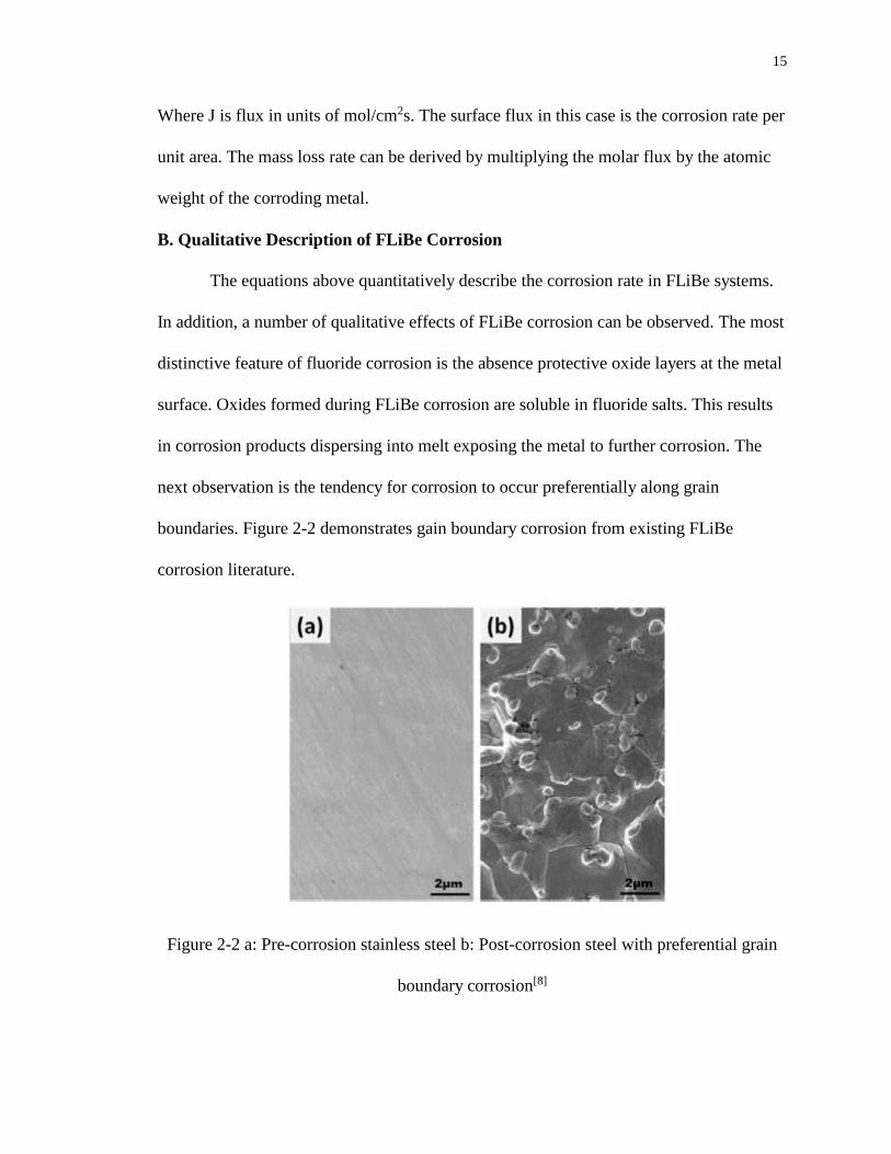
boundaries. Figure 2-2 demonstrates gain boundary corrosion from existing FLiBe

corrosion literature.

Figure 2-2 a: Pre-corrosion stainless steel b: Post-corrosion steel with preferential grain

boundary corrosion[8]

16

When FLiBe is introduced to a system the most reactive alloying element, typically

chromium, reacts with the FLiBe and is depleted from the metal surface. At this point the

corrosion would cease unless more chromium becomes available to react with FLiBe at

the surface. The depletion of chromium at the surface of the metal creates a chromium

concentration gradient that drives solid metal diffusion of chromium to the metal surface.

Chromium diffuses faster along grain boundaries than within metal grains.[8] This results

in the grain boundaries functioning as express lanes for chromium to reach the surface

and react. Because of this, it is expected that materials with finer grain structures will

corrode faster in FLiBe than metals with courser grain structures.

All together metal corrosion in FLiBe is a complex prosses that depends on

electrochemical equilibrium between the salt, structural material, and any present

contaminates. When fluid flow is added to the corrosion system the process becomes

even more complex. Because of this complexity, experimental testing is essential to better

understanding how all of these factors interact during FLiBe corrosion.

17

Chapter 3: Experiment Loop Design and Construction

1. Experiment Overview and Requirements

The goal of the flowing FLiBe corrosion experiment is to test the effects of

laminar flow on metal corrosion in FLiBe. This entails exposing metal samples to

constant flow conditions for 1000 to 3000 hours. By necessity this means that the

experiment must be able to maintain a constant flow velocity and temperature for the

entirety of a test run with minimal operator oversight. The following is the list of design

requirements and constraints for the corrosion test loop.

The first major constraint is the availability of FLiBe. FLiBe must be specially

prepared at Oak Ridge National Laboratory and is only available in small quantities.

Thus, a key design constraint is that the loop must be able to run with 1.2 liters or less of

FLiBe in the system. The second design requirement is that the loop must produce

Reynolds Numbers of up to 2300, the limit of laminar flow, in the system. Third the

experiment must be able to independently control temperature and flow rate so as not to

have a temperature gradient that affects the corrosion rate. Lastly, due to safety concerns

with handling beryllium and fluoride salts the whole facility must be contained to prevent

exposure to the operator and others in the laboratory. Together these four requirements

drive the experimental design.

2. Loop Engineering Design

At the very start of the design process the need to independently control

temperature and flow rate ruled out a convection loop for the experiment, so from the

start a forced convection loop with a pump was decided on. Additionally, it was decided

that the entire experiment would be contained within a glovebox to prevent outside

18

exposure to beryllium. As an added bonus, the glovebox would also allow for precise

control of the oxygen and water levels within the experiment. With the third and fourth

design requirements resolved, the design process continued on the basis of minimizing

the system volume and reaching the desired flow conditions.

A. Loop Dimensions Selection

At this point in the design process the two remaining design drivers were the

volume limit and the need to provide adequate fluid flow. Figure 3-1 outlines the design

process used for the loop.

Figure 3-1 Design Process Flow Chart

The common design element between the two design drivers was what diameter of the

loop tubing. The purpose of the test loop is to replicate the flow conditions found in a

MSR. For the design, laminar flow is sought at Reynolds numbers under 2300. The well

known equation for the Reynolds number is as follows:

19

Where Re is the Reynolds number. is the density. V is the fluid velocity. D is the

characteristic diameter. And lastly is the viscosity. For the fluid flow analysis the

temperature dependent density and viscosity were found in literature and are shown in

equations 3-1 and 3-2.[5]

(3-1)

(3-2)

For the purpose of the preliminary design an operating temperature of 650oC or 923K was

selected.

The first step in selecting a tubing diameter was calculating the relationship

between flowrate, pipe diameter and Reynolds number. Figure 3-2 shows flow rate in

different diameter pipes while Re is held constant. As one would expect flow rate drops

as the pipe diameter increases and as Re decreases.

0

0.2

0.4

0.6

0.8

1

1.2

0 0.005 0.01 0.015 0.02 0.025 0.03 0.035 0.04

Vel

oci

ty (

m/s

)

Pipe Diameter (m)

Pipe Diameter Vs. Flow Speed at Constant RE

1/8" 1/4" 3/8" 1/2"

3/4" 1" 1 1/4"

Figure 3-2 Relationship between fluid velocity and pipe diameter at constant Re

Re: 2000

Re: 1500

Re: 1000

20

Next while deciding on the appropriate system length special attention had to be placed

on the overall system volume. The test loop consists of a melt tank with a pump which

pushes the FLiBe through the test loop. The preliminary design assumed that 40% of the

total volume of FLiBe in the system would be in the melt tank while the loop is operating

to prime the pump. The next step for sizing the system was to calculate the maximum

tubing length for each pipe diameter that resulted in 0.7 L (60% of 1.2 L) of FLiBE in the

loop. Figure 3-3 shows the maximum length of pipe of various diameters that can be

filled with the allotted FLiBe volume. US industry standard pipe diameters are indicated

on the chart for reference. For the design it was decided that at least one meter of loop

length was needed to accommodate the samples and other instrumentation. Based on the

calculated results, tubing one inch in diameter or less would work.

Figure 3-3 Constant Volume Pipe Length

The last sizing parameter to be considered was the pumping power needed for the system.

Equations 3-3, 3-4, and 3-5 were used to derive the pumping power.

(3-3)

21

Where is pumping head from pipe length. Re is the Reynolds number. L is the tubing

length. D is the characteristic diameter. V is the flow velocity. And lastly g is the

gravitational acceleration.

(3-4)

Where is the fitting friction head. K is the resistance coefficient for the fittings.

V is the flow velocity. And g is the gravitational acceleration.

(3-5)

Where W is the pumping power. is the mass flow rate. g is the gravitational

acceleration. h is the elevation head. and are the pipe length and fitting

friction head.

With these equations the pumping power need for the loop design was calculated.

The results of this calculation are shown in figures 3-4 and 3-5. The results assume a 60%

pump efficiency and 90% motor efficiency. From the figures it should be noted that even

in the worst-case scenario the loop needs less than three watts of pumping power to

operate under laminar conditions, so it was deemed that pumping power was unlikely to

be the limiting parameter. Ultimately a ½ horsepower (373 watt) motor was ordered to

power the pump well exceeding the minimum power requirements.

22

Figure 3-4 Diameter dependent pumping power at various Reynolds numbers

Figure 3-5 Diameter dependent starting pumping power at various Reynolds numbers

After completing all of the above calculations and consulting with the tubing supplier, the

pipe diameter of 3/4 inches was selected. The associated length limits and needed

pumping power were used for selecting and designing the loop components.

23

B. Loop Component Description

Figure 3-6 shows the model of the loop with all of its components listed. Table 3-

1 outlines the key specifications of the experiment loop. This section describes the design

for each component in detail.

Figure 3-6 Flowing FLiBe corrosion experiment loop

1: Flow Meter

2: Expansion Tank

3: Pump

4: Melt Tank

5: Electrodes

6: Thermocouples

7: Tubing

8: Fittings

9: Heating Tape

10: Sample Holder

24

Table 3-1 FLiBe Loop Specifications

Operating Temperature 700 ͦC

Loop Length 36”

System Height 36”

System Foot Print 18” x 18”

Operating Volume 1.2 L

Operating Reynolds Number 500-2000

Instrumentation 3 x thermocouples

3 x electrodes

1 x flowmeter

a. Flow Meter

The goal of the flowing FLiBe corrosion test loop is to measure the effect of fluid

flow on metal corrosion in a molten salt environment. To this end the flow conditions in

the loop must be known so that the flow rate and the corrosion rate can be correlated.

Thus, a flow meter was included in the loop to directly the fluid flow. When looking for a

flow meter suited for the system, a problem arose. Currently there are no flow meters on

the market that are both capable of operating at 700 ͦC and small enough to be connected

to the loop. Available high temperature flow meters are designed to be included in large

industrial processes and are therefore too large to be included in the loop without

dramatically increasing its size and volume. Due to the test run FLiBe volume limit this

was not possible. The solution to this problem was to calibrate the pump with a water

flow meter and a water shakedown test. The flow meter is used during the initial water

25

shake down test to measure the correlation between pump controller frequency and the

flow rate. The water flow meter was used during the initial shakedown and then removed

for the molten salt tests.

The flow meter used for the experiment is an Omega FTB-1400 flow meter with a

FLSC-C3-LIQ signal conditioner. The flow meter is shown in figure 3-7.

Figure 3-7 Omega FTB-1400 flow meter with signal conditioner

The flow meter outputs the flow rate as an analog current signal proportional to the

volumetric flow rate. This signal is logged by the experiment’s LabVIEW program.

b. Expansion Tank

The expansion tank consists of three parts: the tank itself, the lid, and the gasket

between the tank and lid. The expansion tank is located at the top of the loop and was

designed to address several experimental needs. It is the primary point of access to the

interior of the loop. The experiment samples are load through the expansion tank and

26

mounted to the expansion tank lid by a threaded holder. The lid is also ported for a

thermocouple and three electrodes. All voltammetric analysis will be performed in the

expansion tank.

The expansion tank is constructed out of 316 stainless-steel. To protect the

stainless-steel from FLiBe corrosion, the interior of the expansion tank will be

electroplated with nickel before used in FLiBe corrosion experiments. The body of the

tank and the tank lid were machined at UNM by the mechanical engineering department

machine shop. The tank is 2” tall, 2” wide, and is 3 ¾” long. The tank also has a 5 5/8” by

3 7/8” flange. Welded to the tank are two Swagelok 1” weld fittings for connecting the

expansion tank to the loop itself. The tank lid is ½” thick and is 5 5/8” by 3 7/8” like the

tank flange. The lid has one thermocouple and three electrode ports. The thermocouple

port consists of a SS316 Swagelok ¼” bore-through fitting. On the interior of the lid the

threaded sample holder mount is concentric with the thermocouple port. The electrode

ports consist of three SS316 Swagelok 1/8” bore-through fittings. The expansion tank

gasket was manufactured at Hennig Gasket company and was made from Pyro-Tex sheet.

Pyro-Tex is a high temperature gasket material made of woven stainless-steel leaf spring

sheathed in graphite. The gasket material was selected because it is rated for up to

1000 ͦC operations, and graphite is inert when exposed to FLiBe. Figures 3-8, 3-9, and 3-

10 are pictures of the expansion tank, the ported lid, and the Pyro-Tex gasket

respectively. The picture of ported lid was taken after the high temperature molten salt

shakedown hence the discoloration and debris.

27

Figure 3-8 Expansion Tank

Figure 3-9 Ported Expansion Tank Lid

28

Figure 3-10 Pyro-Tex Expansion Tank Gasket

c. Pump and Melt Tank

Conducting the flowing FLiBe corrosion experiment requires a heating system to

melt the salt and a pump to push the fluid through the loop. These functions are combined

in the integrated pump and melt tank. The pump and melt tank were designed and

constructed by Wenesco Inc. to the specifications required for the loop.

The melt tank is 6” in diameter, 7” deep, and constructed from 316 stainless-steel.

The melt tank is contained within a 20” x 20” x 15” housing with an integrated 7000W

heater. The melt tank is capable of heating its contents to over 700 ͦC and is controlled by

the connected control box. A nickel 201 pot liner will be installed to protect the melt tank

from corrosion during FLiBe testing.

The pump is a centrifugal design constructed with a SS316 impeller and housing.

The pump impeller assembly fits within the melt tank in order to draw in the melt for

pumping. The pump is powered by a ½ horsepower electric motor with a VFD controller

housed in the control box. The pump is rated for 0.15 gpm at 5 ft of pumping head; this

29

converts to roughly .141 W of power. Figure 3-11 shows the pump and melt tank with the

rest of the loop installed.

Figure 3-11 Pump and Melt Tank

The pump is mounted to the 16” diameter melt tank lid. The lid has four 3/8” NPT ports

and one ½” NPT sampling port. Two of 3/8” ports serve as the pump outlet and return

ports. Figure 3-12 shows the layout of the various melt tank lid ports.

30

Figure 3-12 Melt Tank Lid Port Layout

d. Electrodes

The use of voltammetric analysis to characterize molten salt corrosion was first

demonstrated in the seventies during the MSR program.[10] Voltammetric directly

measures the amount of impurities in the salt. During voltammetric analysis a series of

electric potential are applied to the solution. As the potential becomes large enough to

separate the components of a metal fluoride the current increases as salt constituents

move towards the anode and cathode. By noting the voltages and current the species and

quantity of impurities in the melt can be measured. Voltammetric analysis allows for

continuously observing the change of salt composition during the experiment. This in

turn will allow for correlating the corrosion rate with the salt composition. More recent

work done in the Czech Republic demonstrated a nickel, tungsten, and glassy carbon

31

three electrode effectively measured the voltammetry in FLiBe.[9] will be used to preform

electrochemical analysis on the FLiBe during operations. For the FLiBe corrosion test

loop 1/8” nickel, tungsten, and glassy carbon electrode rods are installed through the

expansion tank lid to perform voltammetric analysis during the experiment. The

voltammetric analysis will be controlled by a digital power supply connected to the

experiment’s LabVIEW software.

e. Thermocouples

The flowing FLiBe corrosion experiment aims to determine the effects on

corrosion of isothermal flow. Thermocouples are needed to measure the salt temperature

throughout the loop. Because of the high temperatures and exposure to corrosive FLiBe a

robust thermocouple was needed. For this reason ¼” diameter 6” long Omegaclad K-type

thermocouples manufactures by Omega were selected for use with the experiment. The

large size and the nickel-based shaft alloy will protect the thermocouples during high

temperature operations in FLiBe. There are three thermocouples installed throughout the

loop. Two are installed next to the pump outlet and return and the third is installed in the

expansion tank lid to measure the temperature of the salt exiting the test section. Figure 3-

13 is a picture of the selected thermocouples.

Figure 3-13 ¼” Diameter Omegaclad K-type thermocouple

32

d. Tubing and Swagelok Fittings

The loop itself is constructed from 1” OD ¾” ID stainless steel tubing and

stainless-steel Swagelok fittings. Eventually the stainless-steel tubing will be replaced

with a Nickel 201/ Inconel 800H bimetallic alloy tubing of the same dimensions for the

FLiBe testing. The tubing and fittings are rigid enough for the loop to be self-supporting.

There are six tubing sections used in the loop each cut to size in the lab. Two 13” upright

tubes are located between the pump connecting fittings and the expansion tank. The pump

outlet side upright is the test section of the experiment. Samples mounted in the sample

holder are suspended in this section and exposed to the fluid flow. The overall length of

this section was selected to allow for the flow to stabilize after the fitting transition and

accommodate multiple experiment samples. The remaining four tubes are 2.5” connector

sections for joining 1” Swagelok fittings to each other.

The Swagelok fittings serve to connect the loop to the pump, act as instrument

ports, and offset the loop from the pump motor assembly. Swagelok fittings were selected

for their ease of installation and the familiarity that those involved in the design had with

them from other projects. The fittings form two distinct groups. The weld fittings were

welded to the expansion tank and lid for loop connections and instrument ports. All the

other fittings were used together to transition from the pumps 3/8” NPT fittings to the

uprights. These fittings include a 45-degree section to offset the loop from the pump

motor assembly. They also include two ports for thermocouples. Table 3-2 lists all the

Swagelok fittings used in the loop. The transition assembly fittings are listed in assembly

order from the pump to the uprights. Before the FLiBe testing, all stainless-steel loop

33

components will be nickel plated to protect against FLiBe corrosion. Lastly figure 3-14

provides a picture of the assembled tubing and fittings.

Table 3-2 List of Swagelok Fittings

Quantity Type

Expansion Tank Fittings

2 1” Male Weld Fitting

1 ¼” Male Weld Fitting

3 1/8” Male Weld Fitting

Pump to Upright Transition Assembly

2 3/8” to ½” Male Tube adaptor

2 ½” 90 ͦUnion Elbow

2 ½” Socket Connector

2 ½” 45 ͦUnion Elbow

2 ½” to 1” Reducer

2 1” to ½” Reducing Tee Union

2 ¼” to ½” Reducer

2 1” 45 ͦUnion Elbow

34

Figure 3-14 Loop of Assembled Tubing and Fittings

35

e. Heating Tape and Insolation

It is of special concern that the temperature in the test section of the loop be

maintained at a constant temperature. To this end a heating tape is mounted around the

test section of the loop to maintain a constant salt temperature around the samples. The

heating tape is an ultra-high temperature ½” by 2’ tape from Omega that is rated up to

1400 ͦF or 760 ͦC which is above the 700 ͦC operating temperature. The heating tape is

controlled by the LabVIEW software. The heating tape can be seen installed around the

sample section in figure 3-11. In addition to the heating tape, the entirety of the

experiment loop is wrapped in Lynn Manufacturing Superwool insolation to reduce heat

loss to the surrounding atmosphere.

f. Sample Holder

The sample holder is mounted to the expansion tank lid and is designed to hold

the material samples being tested. The sample holder is a foot long and has space for nine

samples. The holder consists of two separate slotted brackets joined by a segment of 1/8”

rod. The sample holder is designed for 1” x .565” x .125” samples. The holder and

samples were manufactured at the UNM mechanical engineering machine shop. The

sample holder fits snuggly in the ¾” tubing to prevent the holder from vibrating during

testing. Over the course of the experiment samples will removed one at a time for post

experiment characterization. Each sample will become a snap shot of the material

microstructure at the time of removal. The lowest sample in the holder will also be

subjected to the boundary layer evolution allowing for analysis of the effect of boundary

layer thickness on corrosion in a single sample. The leading edge of the samples and

sample holder was modeled with CFD software to select a holder design that minimized

36

the sample holder’s impact on leading edge’s flow profile. Figure 3-15 is a picture of the

completed sample holder mounted to the expansion tank lid. Figure 3-16 shows the CFD

results for the sample holder leading edge.

Figure 3-15 Sample holder with samples

37

Figure 3-16 CFD model of sample holder

g. Glovebox

In order to protect the experiment operator from beryllium exposure as well as to

prevent contaminating the lab space, a glovebox for the loop was ordered from Vigor

Tech. The glovebox is filled with an inert atmosphere of argon. The argon atmosphere

prevents the introduction of oxygen and water moisture as corrosion agents to the FLiBe.

The internal atmosphere conditions are monitored by a moister and an oxygen sensor. The

glovebox has a sophisticated purification system that actively removes oxygen and water

vapor from the glovebox. The purification system also includes HEPA filters that capture

any beryllium particulate released into the glovebox. Two airlocks are included to allow

for moving materials into and out of the glovebox without introducing outside air. Work

38

in the glovebox is conducted using the two sets of gloves in the front windows. The

glovebox has a built-in air conditioner to remove heat given off by the experiment. Figure

3-17 shows a CAD model of the glovebox.

Figure 3-17 Glovebox Model

The glovebox also has a well for the melt tank. The well is sized to allow for mounting

the melt tank below the glovebox floor. To operate electrical equipment and sensors

inside the glovebox, specially designed feedthroughs are connected to the various power

lines. The glovebox feedthroughs are as follows:

• Feedthrough for melt tank electrical lines

• Feedthrough for pump electrical lines

• Feedthrough for electrochemical lines

• Feedthrough for glovebox power strip

• Feedthrough for thermocouple lines

• Gas feedthrough for pressurized argon line

39

3. Loop Construction

The construction of the experiment began with ordering the pump and melt tank

as well as the glovebox from their respective manufacturers. Next the expansion tank and

sample holder were ordered from the machine shop. The remaining components

mentioned above were also ordered at that time. A new 40A 240V outlet for the pump

and melt-tank was installed in the lab by UNM facilities. Assembly of the loop began

with the delivery of the pump and melt tank from the manufacturer. At this point the

fittings, tubing and instrumentation were put together. The first change made to the loop

was the addition of two ½” 90-degree elbow fittings. The new fittings were need for the

loop to clear the pump mounting structure. Figure 3-18 shows pictures of the assembled

loop as well as pictures of the loops various components.

Figure 3-18 FLiBe loop and component pictures

40

With the loop assembled an outside contractor was brought in to program the LabVIEW

program for the experiment. The LabVIEW software manages the flow meter, electrodes,

heating tape, and thermocouples. The software logs the data from all of those instruments

as well. The software will be used to monitor and manage the test loop for the entirety of

the months long experiment runs. Figure 3-19 shows the interface for the LabVIEW

software.

Figure 3-19 LabVIEW software

The next major construction item was assembling the glovebox after its delivery. A Vigor

Tech technician came to UNM and assembled the glovebox over the course of three days.

At this time the loop was moved into the glovebox and system integration began. Figure

3-20 shows the assembled glovebox. The full integration of the loop with the glovebox

was delayed by a missing feedthrough for the thermocouple lines.

41

Figure 3-20 Fully Assembled Glovebox

After the glovebox assembly and testing, it was opened up for shakedown testing of the

loop. The shakedown tests started with the water and pump calibration test and was

followed by the high temperature molten salt test. Between these tests the flow meter was

removed, and insolation was installed. Figure 3-21 shows the loop in its salt shakedown

configuration with insolation installed. Figure 3-21 shows the assembled loop

configuration at the time of writing.

42

Figure 3-21 Test loop in salt shakedown configuration

4. Loop Shakedown Testing

A. Water Shakedown Test

The first test of the loop was to operate it with water as the circulating fluid. The

goal of the test was to verify that all of the loop components functioned and to measure

the correlation between VFD controller frequency and pumping power. When the test

43

began the pump worked as designed, pumping water through the loop. The data log was

started and the flow rate was measured as the pump control frequency was increased from

20 to 60 Hz in 10 Hz increments. At this point it was confirmed that the system runs

properly with the designed 1.2 L fluid inventory. Unfortunately, the flow meter didn’t

function as intended rendering the flowrate data unusable. Because fixing the flow meter

wasn’t possible at the time and alternate pump calibration method was devise.

For the new pump calibration testing the loop was removed from the pump and

tubing was ran from the pump outlet to an empty container. To measure the mass flow

rate, a timer was running while water was pumped into the container. With the pumping

time and the change in container mass the mass flow rate could be calculated. In turn the

pumping power can be calculated from that mass flow rate. The pumping power equation

(3-5) introduced earlier in the chapter was used for this purpose.

(3-5)

In order perform the calculation the head values in the above equation had to be found.

There was no elevation head so the first h in the equation could be dropped. The testing

set up also only consisted of a single length of tubing, so the fitting head could be drop

from equation 3-5. The only head value remaining was the friction head calculated form

equation 3-3.

(3-3)

To solve for the friction head a conversion between mass flow rate and flow velocity was

need. Equation 3-6 is this conversion.

(3-6)

44

v is the fluid velocity. ṁ is the mass flow rate. ρ is the density. A is the tube cross

sectional area. Equation 3-6 and 3-3 were substituted into equation 3-5 and then

simplified to produce equation 3-7 which is a mass flow rate dependent pumping power

equation.

(3-7)

Where P is the pumping power in watts. L is the length of the tubing in meters. μ is the

viscosity in Pa*s. ṁ is the mass flow rate in kg/s. ρ is the density in kg/m3. And lastly D

is the tubing diameter in meters. For the pump calibration test the length of the tube was

71” (1.8 m) and the tubing diameter was ¼” (.00638 m). Table 3-3 lists the calibration

test results as well as the calculated mass flow rate and pumping power. The 50 Hz data

was lost due a test procedural error.

Table 3-3 Pump Calibration Results

Frequency (Hz) Time (s) M (kg) ṁ (kg/s) Power (W)

20 48.16 0.65 0.0135 0.00737

30 36.61 0.75 0.0205 0.01698

40 25.62 0.6 0.0234 0.02219

60 39.4 1.4 0.0355 0.05109

The data from table 3-3 is plotted in figure 3-22. From the plotted data a best fit equation

was derived. This equation (3-8) is the frequency dependent pumping power for the pump

and is valid from 20Hz to 60Hz.

(3-8)

45

This pumping power equation will be used in conjunction with equation 3-8 as well as the

physical properties of the salt to calculate the flow rate during high temperature

experiments.

Figure 3-22 Frequency Dependent Pumping Power

B. Molten Salt Shakedown Test

The goal of the molten salt shakedown test was to test the experiment facility at

near FLiBe operating conditions as well as acquire some initial flow accelerated corrosion

data. For the test an alternatively salt was needed which wouldn’t require the same safety

procedures as FLiBe. The salt selected was HITEC salt. HITEC salt consists of a mixture

of potassium nitrate, sodium nitrite, and sodium nitrate. HITEC salt is used as a heat

transfer fluid and is know for its application in solar power. The salt melts at 142C and

can operate safely at over 500C making it a suitable material to test the loop facility at

high temperatures. In addition, unlike FLiBe, HITEC salt is generally safe to handle with

46

minimal safety equipment. Gloves should be worn during handling to avoid skin

irritation, and the salt shouldn’t be ingested.

For the test the salt was loaded into the melt tank by hand through the ½” port in

the melt tank lid. Figure 3-23 shows the HITEC salt as delivered. The salt is white in

color and besides a few large clumps consisted of small grains of salt.

Figure 3-23 HITEC salt

Before the test a stainless-steel sample was prepared for corrosion testing. The sample

was cleaned, its dimension taken, and weighed before being loaded into the loop. The

shakedown test would last for 48 hours and any changes in the sample due to corrosion

would be measured.

After loading the sample and the salt, the shakedown test was started. Over the

course of three hours the salt was brought up to 500C melting it. Over the course of the

heating period no issues were observed. Next the pump was turned on and spun up to

operating at full power with a controller frequency of 60 Hz. The loop pumped the high

47

temperature salt without issue. The temperature of the salt remained constant throughout

the insolated loop section. Based on the observed insolation performance, the heating tape

is not necessary to maintain isothermal conditions around the samples. Therefore, the

heating tape can be omitted from future configurations of the experimental loop. After

observing the facility function perfectly for over an hour, the operator left the lab while

the loop continued to run for its 48-hour shakedown test. Unfortunately, a few hours later

the circuit breaker to the facility tripped terminating the test. Attempts to reset the breaker

demonstrated that it would trip even without running either the pump or melt tank

heaters. This suggests that it is a lab electrical system problem and not a problem with the

flowing FLiBe corrosion test loop. An electrician will be needed to determine the exact

issue.

(a) Test Sample Results

Before the shakedown test a stainless-steel sample was cleaned, measured, and

weighed. The dimensions of the sample were measured with calipers and the weight

measured on a high accuracy digital scale. Table 3-4 list the before and after

measurements of the sample exposed to 500 ͦC HITEC salt for several hours.

Table 3-4 Salt shakedown sample changes

Pretest Post-test

Width 0.530 in 0.530 in

Length 1.450 in 1.450 in

Thickness 0.120 in 0.120 in

Mass 8.11308 g 8.11341 g

48

The results in table 3-4 show that no measurable change to the sample dimensions

occurred. Figure 3-24 shows a picture of the post test stainless-steel sample next to an

untested sample.

Figure 3-24 Post test sample next to unused sample

The only discernable difference between the exposed and unexposed sample is the

discoloration of the test sample. This discoloration is most likely surface oxidation which

in turn explains the small weight gain the sample experienced. Longer high temperature

testing in flowing molten salt will be needed to determine any corrosion effects.

(b) Post Test System Inspection

After the molten salt shakedown test, the corrosion loop was disassembled and

had its insolation removed for inspection. During disassembly points of salt leakage were

noted by the insolation that adhered to those areas. The first change to the system noted

was the uniform brown discoloration to the stainless-steel. At 500 ͦC the steel appears to

49

have lightly oxidized giving it its new light brown hew. Figure 3-25 shows the

discoloration of the metal clearly.

Figure 3-25 Post salt shakedown test loop

The first location noted to have leaked salt was the around the expansion tank.

The salt had leaked through the gasket and solidified after seeping into the surrounding

insolation. Figure 3-26 shows the salt that leaked through the gasket cementing some of

the insolation to the expansion tank. To investigate the leakage the lid was removed from

the expansion tank to inspect the gasket. Figure 3-27 shows the gasket and the interior of

the expansion tank. It was first noted that a layer of salt was deposited on the bottom of

the expansion tank. This could be a potential contamination issue in the future. The

gasket itself seemed unchanged from the test. This indicates that the salt flowed around

the gasket to leak. Base on this observation the thickness of the gasket used in future test

will have to be increase. The current gasket wasn’t thick enough to maintain a proper seal

after thermal expansion, so a design correction is needed.

50

Figure 3-26 Salt leakage around expansion tank gasket

Figure 3-27 Post test expansion tank interior and gasket

51

The second leak location was around the first 1” Swagelok socket joint after the

pump outlet. The leak site is shown in figure 3-28.

Figure 3-28 Pump outlet loop leg salt leak site

Once again, the leakage stopped after hardening in the insolation material. It appears that

as a general principle molten salt leaks from the test loop self-seal once a finite amount of

salt has hardened in the insolation. The cause of the leak was in adequate tightening of the

Swagelok fitting in combination with the pressure of the pump outlet. To prevent future

leaks of this type failed joints will be retightened and extra care will be taken when

reassembling Swagelok joints.

The last and largest salt leak was from around the melt tank. A significant amount

of salt had leaked through melt tank lid gasket and started to flow down the exterior

housing. Figure 2-29 shows the leak around the melt tank.

52

Figure 2-29 Melt tank leak

After inspection it was also noted that the gasket itself was infused with HITEC salt. The

cause of this leak was poor loading technique. During loading, salt grains piled up on the

pump impeller till the pile reached the melt tank rim at which point some of the salt

accumulated on top of the melt tank housing. After melting this free salt began to flow

resulting in the leakage seen in figure 2-29. Care will be taken when loading salt in the

future to prevent future leaks. One option is to load from the opposite side of the melt

tank to avoid salt being deposited on top of the impeller.

All together the test loop performed well during the molten salt shakedown test,

and all of the salt leaks have been addressed.

53

Chapter 4: Flowing FLiBe Corrosion Model

1. Current Models and Their Limits

A key mark of understanding a physical process is the ability to accurately predict

the outcome of the process when the starting conditions are known. Such understanding

also aids design work by reducing the need for full scale prototyping tests. In the case of

flowing FLiBe corrosion, the development of an accurate numerical corrosion model

properly validated by experimental results would allow for rapid exploration of the FLiBe

design space. The results of such a model would point towards promising solutions to

design challenges and support experimental work by providing a more focused testing

matrix. For these reasons a multi-physics numerical model of flowing molten fluoride salt

corrosion was developed.

Much of the early work with flowing molten salt corrosion took place in

conjunction with the Molten Salt Reactor experiment at Oak Ridge National Lab. Much

of the supporting corrosion research focused on creating a library of corrosion tests for

various materials in a thermal convection test loop.[10] While creating a reference pool of

experiments is essential for doing further design work, predicting results not directly

tested requires a theoretical framework for extending the results. Since the early loop

tests, corrosion models have been created in support of later static FLiBe corrosion tests.

These models have typically consisted of a single governing equitation that models a

single phenomena. One example is the model used for predicting chromium concentration

at increasing depths inside a metal sample exposed to FLiBe. Equation 4-1 works on the

assumption that the surface concentration of Cr remains constant at zero and thus Cr loss

depends only on internal diffusion.[8]

54

(4-1)

Equation 4-1 effectively correlates to its paper’s results but is incapable of accounting for

any corrosion regime besides metal diffusion limited corrosion.

Another example of a FLiBe corrosion model is the electrochemical model

governed by Butler-Vomer equation shown in a paper produced by Virginia Tech.[7] This

model calculates the corrosion rate based on the electrochemical reaction that occurs at

the metal salt interface. (A more detailed explanation of this method is explained later in

the chapter.) While the mentioned paper includes methods for accounting for mass

transport and diffusion limited cases the model remains primarily focused on the surface

reaction.

A common feature of existing FLiBe corrosion models is the focus on a single

physical process. That process could be alloy element diffusion in metal or

electrochemical reactions at the metal salt interface, but the generalization of each model

is limited to the cases where the modeled process is the limiting case. A general model

with wide applicability must take into account multiple physical processes that influence

the corrosion.

The newly created FLiBe corrosion model overcomes the limitations of previous

models by calculating the solid metal diffusion, surface reaction, and mass transport

simultaneously.

55

2. Model Implementation

A. Overview

Fluoride salt corrosion is distinguished from other typical corrosion conditions by

the lack of a passive oxide layer. For corrosion systems, such as in air or water, metal

oxides form on the surface of a metal protecting it from further oxidation. In fluoride salt

melts such corrosion products dissolve into the melt instead of forming a passive layer.[2]

This in turn results in consistent corrosion at the metal salt interface uninhibited by

passive oxide layer.

To accurately model fluoride salt corrosion under flow conditions, three separate

physical phenomena must be accounted for. The first phenomenon is the diffusion of

alloying elements through the metal to the surface. The second phenomenon is the

irreversible electrochemical reaction that occurs at interface between that metal and the

melt.[7] The last phenomenon is the mass transport of reactants from the melt bulk to the

metal surface. Previous models focus for the most part on one of the above phenomena. A

general model requires each of the above processes and their interactions to be accounted

for.

In the subsequent sections the implementation of each process will be explained.

In section B solid metal diffusion is modeled by Fick’s second law implemented in an

implicit finite difference method. In section C the surface reaction is modeled with

Butler-Vomer electrochemical equation. In section D the mass transfer is calculated based

on Sherwood number correlations. Section E explains the algorithm for coupling each of

the physical phenomena. Section F verifies the performance of the model by

56

demonstrating diffusion, surface reaction, and mass transport limited cases. Section G

contains the validation of the model against experimental results.

B. Alloy Element Diffusion in the Solid Alloy

According to Fick’s hypothesis diffusion is a mass transfer process proportional to

the concentration gradient. This hypothesis is summarized by Fick’s first law (eq. 4-2)

F = -D δC/δx (4-2)

F is the rate of mass transfer over area. D is the diffusion coefficient. C is the

concentration. Lastly x is length.

The diffusion equation is further derived in three dimensions by considering the

case of a rectangular parallelepiped whose sides are aligned with the major axes and the

length of the sides are 2dx, 2dy, and 2dz. The concentration of the diffusing substance is

C. The rate of which the substance enters one of the x perpendicular faces is:

Fx is the rate of transfer through the side. The equation for the other x perpendicular face

is:

When combined the net flux in the x direction is:

The equations in the y and z directions are of the same form. The rate the substance

increases in the volume with time is:

8dxdydz

57

By combining each term, the concentration in the volume is defined by:

By substituting Fick’s first law for each of the above flux terms Fick’s second law, the

diffusion equation, is derived.

Or when simplified to be one dimensional.

(4-3)

Fick’s second law (eq. 4-3) is the equation used when solving for the time dependent

concentration in the model.

Fick’s second law can be solved analytically for simple cases, however numerical

methods are required for more complex cases such as multiple material layers. The

numerical method selected is the implicit finite difference method. Said method benefits

from not having a solution stability limit. The method works by discretizing a material

into a series of nodes of a finite size. Fick’s second law is then solved for the boundaries

of each node. This allows for the calculation of the concentration across discontinuities as

well through multiple materials. Equation 4-4 is an example of Fick’s second law

discretizes for the implicit finite difference method.

(4-4)

C is the concentration in moles. p is the timestep counter while n is the node location. D1

is the diffusion constant of the material in m2/s and Δx is the distance between each node.

58

The mass balance equation is then rearranged to group the Cn-1p+1, Cn

p+1, and Cn+1p+1

variables (eq. 4-5)

(4-5)

An important feature of the implicit finite difference method is that the concentrations are

solved for the next time step based on the adjacent concentrations also at the next time

step unlike the forward finite difference method. The implicit finite difference method

generates as system of equations based on equation 4-5. The system of equations takes

the form of AX = B with A being the coefficient matrix, X being the p+1 concentrations

and B being the time step p concentrations. The equation is then solved via matrix

mathematics for X. The equations at the boundaries and any material interfaces much be

adjusted to take into account the relevant conditions. Table 4-1 lists the node equations

used in the implemented model which consists of two materials layered together. The

boundaries are presumed to be impermeable.

59

Table 4-1 Finite Difference Method Node Equations

Region 1

Boundary

Region 1

Interior

Material

Interface

Region 2

Interior

Region 2

Boundary

In order to properly validate the diffusion model a simple one material case

matching existing experimental work was created. The boundary conditions were set as

constant C = 0 for the FLiBe facing surface and dC/dt = 0 for the far surface. These

boundary conditions presume that all Cr reacts as soon as it comes into contact with the

FLiBe and that no Cr leaves through the other surface. The reference results comes from

research conducted at University Wisconsin Madison were stainless steel was exposed to

static FLiBe.[2] Included in the results is equation 4-1, mentioned above, that describes the

time dependent Cr distribution in the stainless steel. The results from the finite difference

method and eq. 4-1 are compared in figure 4-1.

60

Figure 4-1 Finite Difference Method Validation

Figure 4-1 shows that the implicit finite difference method agrees with existing results for

FLiBe corrosion and can be further used to model Cr diffusion.

C. Surface Reaction Model

Metal corrosion in fluoride salts is an irreversible electrochemical reaction that

occurs at the interface of the salt melt and metal.[7] The metal serves as the anode of the

reaction and dissolves into the melt. Oxidants in the salt serve as the cathode and is

reduced. Whether the reaction occurs spontaneously depends on the Gibbs free energy of

formation. Equation 4-6 show the electrochemical Gibbs free energy equation.

ΔG = -nFΔE (4-6)

ΔG is the Gibbs free energy and has units of J/mol. F is the Faraday constant, 96,485

C/mol. n is the number of charges exchanged in the reaction. Lastly ΔE is the potential

difference between the cathode and the anode. If the anode has a smaller potential than

61

the cathode then the reaction occurs spontaneously. In the case of steels the expected

reaction is the reduction of NiF2 (reference potential -2.42 V[7]) and the oxidation of Cr

(reference potential -3.28 V[7]). NiF2 is an impurity of concern in the molten salt while Cr

is a common alloying element in structural metals. The expected result of the

electrochemical process is the deposition of Ni and the dissolution of Cr into the salt.

The electrochemical reduction process for each element is governed by the Butler-

Volmer equation (equation 4-7).

(4-7)

Where i is the current density (A/cm2), io is the exchange current density (A/cm2), α is the

charge transfer coefficient, n is the charge of the ion, F is the Faraday constant, R is the

gas constant, T is the temperature, and η is the overpotential which equals Eelectrode –

Eequilibrium. The electrode potential is the potential actually experienced while the

equilibrium potential is the potential when the reactants are at equilibrium concentrations.

Equation 4-8 is used to calculate the equilibrium potential.

(4-8)

E* is the tabulated formal potential. R is the gas constant. T is the temperature. And C is

the concentration of metal fluoride in the melt and the solid metal in the alloy. Equation

4-9 is the equation for the exchange current density.

(4-9)

Where ko is the reaction rate, C is the bulk concentration in the fluid, and X is the

concentration in the metal. The corrosion rate is determined by calculating the current

density curves for each reactant and finding the electrode potential at which the sum of

62

the current densities is zero, or in other words when the oxidation rate matches the

reduction rate. Current density is related to species flux by equation 4-10.

(4-10)

Where J is flux in units of mol/cm2s. The surface flux in this case is the corrosion, and the

mass loss can be derived from the atomic weight of the corroding metal atoms.

D. Flowing Fluid Mass Transport

In the course of the electrochemical surface reaction, the oxidant salt in the melt is

reduced at the corrosion surface and is depleted. Oxidant salt depleted this way is

replaced by the mass transport of the oxidant from the fluid bulk to the surface. In the

case that the oxidant is depleted faster that it can be replenished via transport, the reaction

becomes mass transport limited. Equation 4-11 is the current density equation for the

oxidant via mass transport.[7]

(4-11)

Where km is the mass transfer coefficient and cb and cs are the bulk and surface

concentration of the oxidant respectively. The maximum mass transport current density

occurs when the melt at the metal surface is completely depleted and surface

concentration becomes effectively zero. Equation 4-12 shows this limiting case.

(4-12)

The transport limited current density shown in equation 4-12 effectively represents the

maximum possible corrosion rate for the system. The corrosion rate can only exceed this

value for the period of time it takes to deplete the surface concentration of oxidant, after

which the corrosion rate promptly drops to the limiting value.

63

Calculating the mass transport limited current density requires that the mass

transfer coefficient for the system be first calculated. This value can be derived from the

Sherwood number for the system which when solved for the mass transport takes the

form of equation 4-13.

(4-13)

Where D is the diffusivity of the oxidant, L is the characteristic length, Re is the

Reynold’s number, and Sc is the Schmidt number. A, α, and β are constants dependent on

the correlation empirically determined for the system. For these values the Dittus-Boelter

equation[11] can be used with the heat-mass transfer analogy. Equation 4-14 shows

equation 4-13 with the Dittus-Boelter equations included.

(4-14)

The equations for the Reynold’s and Schmidt numbers are shown in equations 4-15 and

4-16 respectively.

(4-15)

(4-16)

Where ρ is the density of the fluid, v is the fluid velocity, and μ is the dynamic viscosity.

All together this allows for the calculation of the mass transfer coefficient and in turn the

limiting current density.

E. Model Coupling and Implementation

Having established models for the solid metal diffusion, the surface reaction, and

the mass transfer limit of the surface reaction, these three models must be combined to

64

create a comprehensive model. This section lays out the step by step process of coupling

the models together and lists the constants used and their sources.

The model is an iterative algorithim. This means that the entire model is solved

for one timestep before proceeding to the next. Step one is solving the implicit finite

difference method matrix for the metal concentrations for the time step. Step two is

solving for the exchange current density (equation 4-9) using the surface concentration of

chromium calculated in step one. This step couples the solid diffusion model to the

surface reaction. For step three the Butler-Volmer equation (equation 4-7) is solved for

chromium and nickel (or iron depending on melt impurities) using the exchange current

density calculated in step two. Chromium in the case of typical FLiBe corrosion is the

dissolving anode and nickel (or iron) fluoride is the depositing cathode. To find the

correct electrode potential the solution space of the Butler-Volmer equation is searched.

The first search consists of calculating the results of the Butler-Volmer equation over a

range of expected electrode potentials. Then the electrode potential which produces the

smallest difference between the nickel and chromium current density is selected. A finer

search is then conducted around the previous best electrode potential. This process is

repeated four times. After this process is done step three has produced the current density

for the surface reaction. Step four compares the current density from step three to the

mass transport limited maximum current density calculated based on the flow conditions.

If the current density exceeds the limiting value, the corrosion rate is downgraded to the

mass transport limited value. Step four is the point at which the fluid flow effects are

coupled to the model. Step five consists of converting the reaction current density to a

flux with equation 4-10. Based on the derived flux the mass loss for the time step is

65

calculated and subtracted from the surface concentration of the metal. At this point the

process starts over again at step one. This entire solution is summarized in table 4-2.

Table 4-2 Model Coupling Algorithm

Step 1 Solve implicit finite difference method for Cr concentration in the metal

Step 2

Solve for exchange current density based on surface concentration from

step 1

Step 3 Search for best electrode potential and solve for reaction current density

Step 4

Compare/correct step 3 current density with mass transfer limit current

density

Step 5

Convert current density to a flux and update the metal surface

concentration

The above algorithm calculates the corrosion rate for metal alloys in flowing FLiBe. It

couples the alloy element diffusion in metal and flow effects with the surface

electrochemical reaction to comprehensively model the corrosion. This section finishes

with table 4-3 which lists the constants used in the above algorithm. Unless otherwise

noted the values in table 4-3 are used for all of the subsequent model results.

66

Table 4-3 List of Constants

D Cr in Nickel 9.5e-17 m2/s[12] α Cr 0.32[16]

D Cr in Nickel 2.55e-19 m2/s[13] α Fe 0.09[16]

D Cr in Incoloy

800H

9.415e-16 m2/s[14] α Ni 0.50[7]

D Cr in Incoloy

800H

2.0e-17 m2/s[15] ρ FLiBe @ 700 ͦC 1671.1 kg/m3[7]

D Cr in Incoloy

800H

6.0e-18 m2/s[15] μ FLiBe @ 700 ͦC 5.50e-3 Pa*s[7]

D NiF2 in FLiBe 5.0e-10 m2/s[7] E reference Cr -3.28 V[7]

k0 Cr 2.17e-10 /s*cm2[16] E reference Fe -2.92 V[7]

K0 Fe 5.77e-9 /s*cm2[16] E reference Ni -2.42 V[7]

k0 Ni 5.77e-11 /s*cm2[16,7]

F. Code Verification

After implementing the model, it is necessary to verify that it is performing as

expected. The key features of the model are the alloy element diffusion, surface reaction,

and the flow effect model. In order to verify that the model is acting as expected the

diffusion limited, reaction rate limited, and mass transport limited cases must be

demonstrated to show that each component of the model is capable of impacting the

results. The limiting cases were chosen because differences at the extremes are simplest

to observe. The following three subsections illustrate each of the limiting cases in turn.

67

a. Solid Diffusion Limited Case

In the case that the corrosion rate is limited by the solid alloy element diffusion a

number of phenomena are expected. First, when the diffusivity of the metal decreases the

mass loss rate due to corrosion for the system decreases. Second, the surface

concentration of chromium in the metal will drop to zero because the surface reaction

consumes the Cr faster than it diffuses to the surface.

To verify the model three simulations were run. The first simulation modeled

flowing FLiBe corrosion at typical values and the metal diffusion coefficient was set at

9.415e-16 m2/s (the most diffusion value for Incoloy 800H[14]). The subsequent

simulations were identical to the first except that the diffusion coefficients were set at

9.415e-18 m2/s and then 9.415e-20 m2/s. Figure 4-2 shows the resulting mass loss rates

for the simulations.

Figure 4-2 Mass Loss Rate for Diffusion Limited Verification Case

68

As expected, the mass loss rate for the low diffusivity cases drop off as the surface

chromium is depleted in the reaction and replacement chromium diffuses slowly to the

surface. The mass loss rate continues to drop over time for the limited cases due to the

concentration gradient smoothing out over time resulting in less transport to the surface.

As expected, a lower diffusion coefficient results in the loss rate dropping off faster. For

the reference case, the drop in mass loss rate is due to the drop in overall chromium

concentration in the finite system. Figure 4-3 illustrates the change in the concentration of

chromium in the metal allow over time for the lowest diffusivity case.

Figure 4-3 Cr Concentrations for the Diffusion Limited Case

The shape of the chromium distribution in figure 4-3 demonstrates surface depletion of

Cr. This marks another point of verification that the model behaves as expected when the

69

diffusion coefficient of the alloy is reduced. All in all, this demonstrates that the model

responds properly to changes in the alloy diffusion coefficient.

b. Surface Reaction Rate Limited Case

The reaction rate of the surface reaction directly determines the rate of corrosion

in flowing FLiBe. In the case when the reaction rate coefficient is small, the reaction rate

limited case arises. When reaction rate coefficients for the electrochemical reactions are

reduced the mass loss rate for the model should also decrease. The concentration gradient

in the metal should also remain relatively flat because diffusion in the metal smooths out

any chromium loss in the alloy. Figure 4-4 illustrates the mass loss rate drop that occurs

when the reaction rate coefficients are decreased first to 33% then 10% of their original

value.

Figure 4-4 Mass Loss Rate for Reaction Rate Limited Verification Case

70

As one would expect, the mass loss rate drops significantly when the reaction rate

coefficients are decreased. The mass loss rate for the limited case decreases slower than

the diffusion limited case because the change in surface concentration of chromium drops

much slower. This slow drop in surface concentration is illustrated in figure 4-5 which

shows the concentration gradient for the surface reaction limited case.

Figure 4-5 Cr Concentrations for the Reaction Rate Limited Case

Altogether, the above results show that the model responds as predicted to changes in the

reaction rate at the material surface.

c. Mass Transport Limited Case

In the mass transport limited case oxidants in the melt are consumed at the surface

faster than they are transported there. This produces an effective zero surface

concentration which in turn causes the maximum rate of mass transport between the fluid

bulk and the surface. The surface reaction rate in turn is reduced to the mass transfer rate.

71

Figure 4-6 shows the change in the mass loss rate over time when the flow rate of the

FLiBe is reduced.

Figure 4-6 Mass Loss Rate for Transport Limited Verification Case

Figure 4-6 shows the expect result that the mass loss rate in the transport limited case

becomes constant. This constant rate matches the maximum mass transport possible

under the existing flow conditions. The threshold for the mass transport limited case is

the point at which the available oxidants at the surface can no longer consume all the

surface Cr. Before this point the system is in the diffusion limited case. It should be noted

that even for a two order of magnitude drop in the flow rate the mass loss is only reduced

by about 66%. The diffusion coefficients of the oxidants in the melt are large relative to

the overall corrosion rate. This means that the corrosion of metal in flowing FLiBe would

be expected to show less response to changes in flow conditions. Figure 4-7 is included to

show the chromium concentrations over time for the mass transport limited case.

72

Figure 4-7 Cr Concentrations for Mass Transport Limited Case

The above verification cases demonstrate that the model effectively incorporates the

physics of solid alloy diffusion, electrochemical redox reactions, and mass transport

under flowing conditions.

G. Model Validation

Having verified that the model responds to changes in corrosion conditions in a

physically rational manner, validation of the code against experimental results is required.

The Oak Ridge convection loop experiments referred to in the introduction of this chapter

was selected for model validation. Table 4-4 summarizes the model inputs drawn from

the research paper.[10] All values shown in table 4-4 come from the Oak Ridge paper

except for the stainless-steel diffusion coefficient which was taken from published values.

73

Table 4-4 Validation Case Values

Parameter Value Parameter Value

D 316 SS 4.2e-19 m2/s[7] CFe 1.9e-4

L 0.0254 m T 650 ͦ C

V 0.0167 m/s Mloss 500 hr .45 mg/cm2

CCr 6.0e-5 Mloss 1000 hr .65 mg/cm2

The Oak Ridge experiment was selected as the validation case for several reasons. First,

the experiment exposed metal samples to flowing FLiBe which is exactly the physical

conditions the model was designed to replicate. The overall number of published flowing

fluoride salt corrosion experiments are low, and most of the experiments conducted with

FLiBe flow in tubing were conducted at Oak Ridge. This is part of the reason that there is

currently renewed interest in flowing FLiBe corrosion experiments. Continuing from the

last point, the experiment was conducted in standard tubing. More recent experiments

which include flowing FLiBe corrosion tend to have experimental set ups where the

molten FLiBe is in a flask mixed by an impeller.[4] The mass transport portion of the

model is ill suited to such exotic flow conditions. Lastly, the Oak Ridge paper includes

important values such as the flow speed and geometry as well as the concentrations of

oxidizing contaminants in the salt. All together the Oak Ridge experiment was a natural

choice for the validation case.

Figure 4-8 shows the mass loss results of the model compared to experimental

results. The uncertainty represents the possible unreported contaminates in the salt that

could accelerate corrosion. These uncertain unreported impurities are represented by

adding or taking away from the FeF2 concentration.

74

Figure 4-8 Model Calculated Mass Loss vs Validation Case Values

Overall the model agrees well with the Oak Ridge experiment. Underestimating the 500

hour mass loss is to be expected because corrosion in FLiBe is initial accelerated by

additional contaminants such as water.[2] These starting oxidants are rapidly consumed.

The long term corrosion rate is determined by metal oxidants like nickel and iron

fluoride. Another possible source of uncertainty is the unspecified diffusivity of the

stainless steel samples. Metal diffusion coefficients can vary greatly with microstructure.

In general diffusion along grain boundaries occurs much faster than in grains, thus metals

with finer grain structures also have larger diffusion coefficients.[7] Despite these

challenges, the above result shows that when the physical parameters can be well

matched, the model accurately predicts mass loss.

75

3. Model Applications to the FHR System

Having explained the model’s implementation and demonstrated its validity, its

application to the FHR design is now investigated.

A. Bimetallic vs Single Alloy Materials

One of the areas of investigation for the research connected with this thesis is the

application of bimetallic alloys to fluoride salt systems. The bimetallic alloy consists of

Incoloy 800H coextruded with a pure nickel surface layer. The nickel is intended as

corrosion protection for the underlying structural material. Investigation of such

bimetallic alloys was the primary motivator for designing the FDM method in section 2B

to use multiple material substrates. Extruding the nickel layer as opposed to electroplating

has the additional benefit of creating a nickel microstructure that is more resistant to

chromium diffusion. Electroplating produces a very fine microstructure which in turn

result in a high diffusivity coefficient.[12] These features together promise to produce a

structural material for FHR reactors that is highly resistant to FLiBe corrosion.

In order to investigate the potential benefits of using a bimetallic alloy in an FHR

design, the mass loss rate of bimetallic alloys of various nickel thickness were modeled.

Values from table 4-3 were used for the investigation with 2.55e-19 m2/s and 2.0e-17

m2/s used as the diffusion coefficients for nickel and Incoloy 800H respectively. Figure 4-

9 shows the resulting mass loss rates of bimetallic alloys 5, 10, and 15 micrometers thick

as well as the mass loss rate of bare Incoloy 800H for comparison.

76

Figure 4-9 Mass Loss Rate for Bimetallic Alloy of Varying Ni Thickness

The results show that increasing the thickness of nickel surface layer not only reduces the

mass loss rate for the metal but also delays the onset of corrosion. The nickel surface

layer acts as a barrier to chromium loss. Chromium must first diffuse through the nickel

substrate to the metal surface before it can react electrochemically with the FLiBe. Figure

4-10 shows the development of the Cr concentration profile of bimetallic alloy.

Figure 4-10 Cr Concentration in Bimetallic Alloy (5 μm Ni)

77

Initially in the bimetallic alloy there is no surface chromium as shown with the 15 hour

line in figure 4-10. Over time chromium diffuses into the nickel layer flattening the

concentration gradient throughout the layer as shown in the 2000, 4000, and 6000 hour

plots. The concentration gradient stabilizes as a linear gradient between the metal surface

chromium concentration and the Incoloy 800H Cr concentration develops. The peak mass

loss rate in the bimetallic alloy occurs once this equilibrium concentration gradient is

reached.

All together the above results show the performance advantages a bimetallic alloy

has in corrosion performance. The nickel layer places a cap on the mass loss rate

significantly below that of a bare metal. In the next section a bimetallic alloy is applied to

the mark-1 pebble-bed fluoride high temperature reactor (PB-FHR) to demonstrate the

engineering benefits of bimetallic alloys when applied to an actual design.

B. Bimetallic Alloy Performance Impact on FHR Heat Exchanger Tubes

The Mark-1 PB-FHR pre-conceptual design was produced by UC Berkeley in

collaboration with MIT and the University of Wisconsin, Madison.[1] The design is for a

small modular fluoride salt cooled reactor and includes parameters for the entire reactor

system including the core and heat exchanger system. For this design study the one year

mass loss from the heat exchanger tubes were investigated. The material of the heat

exchanger tubes in the design is stainless steel.[11] The benefits of applying a bimetallic

nickel layer to existing stainless steel was modeled. Table 4-5 lists the values taken from

the mark-1 design; other values were taken from the sources previously listed.

78

Table 4-5 FHR Heat Exchanger Parameters

Parameter Value

OD Tube 6.350 mm

Tube Thickness 0.889 mm

V Flow 1.09 m/s

Oxidant concentrations were taken from the minimum FLiBe purity standards used for

the MSR at Oak Ridge which were 25 parts per million Cr and Ni.[2] The mass loss for

bare 316 SS, a 5 μm Ni layer, and a 10 μm layer were modeled.

Figures 4-11 and 4-12 show the mass loss rate and total mass lost for FHR heat

exchanger tubing.

Figure 4-11 Mass Loss Rate FHR Heat Exchanger Tubing

79

Figure 4-12 Mass Loss for FHR Heat Exchanger Tubing

The one year mass loss was 3.23, 0.34, and 0.013 mg/cm2 for bare 316 SS, 5 μm Ni, and

10 μm Ni respectively. The performance gains from adding a nickel surface laying in the

heat exchanger tubing is substantial. Five micrometers of nickel decrease the mass loss in

the heat exchanger tubing by an order of magnitude. Ten micrometers decreases the mass

loss by two orders of magnitude. Bimetallic alloys have the potential to extend the service

life of an FHR heat exchanger bundle a hundred-fold. Due to limitations in the

manufacturing process, the nickel layer in actual bimetallic tubing is likely to be much

thicker than modeled above. This suggests that actual bimetallic tubing would have even

better performance. With such performance compared to traditional tubing, bimetallic

tubing will likely be lifetime cost competitive against single metal tubing despite its

higher manufacturing cost.

80

All together the modeling work suggests that bimetallic alloys can dramatically

improve the corrosion performance of molten FLiBe systems. Such results give new

impetus for investigating composite materials for use in molten FLiBe systems.

4. Conclusion

The multiphysics FLiBe corrosion model developed in this chapter successfully

models the solid alloy diffusion, surface electrochemical reaction, and the flow mass

transport effects that occur during flowing FLiBe corrosion. The model was verified to

perform as expected and validated against a flowing FLiBe corrosion experiment

conducted at Oak Ridge Nation Laboratory. Further, the model was used to show the

impressive corrosion resistance bimetallic alloys have in flowing FLiBe. All together this

demonstrates the benefits of the developed corrosion model as an engineering tool. This

model will be further validated against the experimental result of the flowing FLiBe

corrosion test loop described in the previous chapters. Altogether, the model described in

this chapter is a valuable tool for designing corrosion resistant materials for molten FLiBe

systems.

81

References

1. C. Andreades, et al, “Technical Description of the “Mark 1” Pebble-Bed Fluoride-

Salt-Cooled High-Temperature Reactor (PB-FHR) Power Plant,” University of California

Berkeley, UCBTH-14-002, 2014.

2. M. Anderson et al, “Heat Transfer Salts for Nuclear Reactor Systems – Chemistry

Control, Corrosion Mitigation, and Modeling,” CFP-10-100, University of Wisconsin,

Madison (2016).

3. H. G. MacPherson, “The Molten Salt Reactor Adventure,” Nuclear Science and

Engineering, 90, 374-380 (1985).

4. M. Kondo, et al, “Flow accelerated corrosion and erosion-corrosion of RAFM

steel in liquid breeders,” Fusion Engineering and Design, 86, 2500-2503 (2011).

5. E. M. Baum et al, Nuclides and Isotopes: Chart of the Nuclides, 17th edition,

Knolls Atomic Power Laboratory, (2010).

6. R. Serrano-Lopez, J. Fradera, S. Cuesta-Lopez, “Molten salts database for energy

applications,” Chemical Engineering and Processing: Process Intensification, 73, 87-102

(2013).

7. S. Guo, J. Zhang, W. Wu, W. Zhou, “Corrosion in the molten fluoride and

chloride salts and materials development for nuclear applications,” Progress in Materials

Science, 97, 448-487 (2018).

8. G. Zheng, L. He, D. Carpenter, K. Sridharan, “Corrosion-induced microstructural

developments in 316 stainless steel during exposure to molten Li2BeF4(FLiBe) salt,”

Journal of Nuclear Materials, 482, 147 (2016).

82

9. M. Straka, M. Korenko, F. Lisy, “Electrochemistry of uranium in LiF-BeF2 melt,”

Journal of Radioanalytical and Nuclear Chemistry, 284, 245-252 (2010).

10. J. Keiser, J. DeVan, D. Manning, “The Corrosion Resistance of Type 316

Stainless Steel to Li2BeF4,” ORNL/TM-5782 (1977).

11. M. El-Wakil, Nuclear Heat Transport, La Grange Park: American Nuclear

Society, 1978.

12. L. Olson, K. Sridharan, M. Anderson, T. Allen, “Nickel-plating for active metal

dissolution resistance in molten fluoride salts,” Journal of Nuclear Materials, 411, 51-19

(2011).

13. C. Smithells, et al, Smithells Metals Reference Book, Ch. 13, Elsevier Science &

Technology, (2003).

14. A.R. Paul, K.N.G. Kaimal, M.C. Naik, S.R. Dharwadkar, “Lattice and grain

boundary diffusion of chromium in superalloy Incoloy-800,” Journal of Nuclear

Materials, 217, 75-81 (1994).

15. T. Ericsson, “A Study of the Cr-Depleted Surface Layers Formed on Four Cr-Ni

Steels During Oxidation in Steam at 600 ͦ C and 800 ͦ C,” Oxidation of Metals, 2, 401-417

(1970).

16. W. Wu, S. Guo, J. Zhang, “Exchange Current Densities and Charge-Transfer

Coefficients of Chromium and Iron Dissolution in Molten LiF-NaF-KF Eutectic,”

Journal of The Electrochemical Society, 164, C840-C844 (2017).