An Experimental Investigation of the Drag on Idealised

An Experimental Investigation of the Drag on Idealised Rigid, Emergent Vegetation and Other Obstacles in

Turbulent Free-Surface Flows. A thesis submitted to the University of Manchester for the degree of Doctor

of Philosophy in the Faculty of Engineering and Physical Sciences

2016

Francis Henry Robertson

School of Mechanical, Aerospace and Civil Engineering

2

Table of Contents

List of Tables .......................................................................................................................... 8

List of Figures ......................................................................................................................... 9

Abstract ................................................................................................................................ 13

Declaration ........................................................................................................................... 14

Copyright Statement ............................................................................................................ 15

Acknowledgements .............................................................................................................. 16

The Author ........................................................................................................................... 17

Notation ................................................................................................................................ 18

1 Introduction................................................................................................................... 24

1.1 Modelling Approach .............................................................................................. 27

1.2 Project Aims and Objectives ................................................................................. 28

1.3 Thesis Scope ........................................................................................................ 30

2 Theory .......................................................................................................................... 31

2.1 The Drag on Isolated Cylinders ............................................................................ 32

2.1.1 The Mean Drag Coefficient ........................................................................... 32

2.1.2 Continuity Principle and Blockage Ratio ....................................................... 33

2.1.3 Reynolds Number ......................................................................................... 35

2.1.4 Root Mean Square Drag Coefficient ............................................................. 36

2.2 Open Channel Flow .............................................................................................. 36

2.2.1 Empirical Friction Laws ................................................................................. 37

2.2.2 Typical Values for Manning’s Coefficient ...................................................... 38

2.2.3 The Froude Number ..................................................................................... 39

2.3 Drag in Cylinder Arrays ........................................................................................ 39

2.3.1 Solid Volume Fraction................................................................................... 39

3

2.3.2 Array-Averaged Drag Coefficient .................................................................. 40

2.3.3 The Definition of the Reynolds Number for Flow through an Array ............... 41

2.3.4 The Site-Specific Resistance Coefficient ...................................................... 44

2.4 Continuity and Navier-Stokes Equations .............................................................. 46

2.4.1 Unsteady Reynolds-Averaged Navier-Stokes (URANS) Equations .............. 46

2.4.2 Modelling Strategy Applied in This Study ..................................................... 47

2.5 Boundary Layers .................................................................................................. 49

2.5.1 Boundary Layer Structure ............................................................................. 51

2.5.2 Flow Separation ............................................................................................ 54

3 Literature Review ......................................................................................................... 56

3.1 The Drag on Cylinders of Various Cross-Sectional Geometries ........................... 57

3.1.1 The Mean Drag Coefficient of Circular Cylinders .......................................... 57

3.1.2 The Mean Drag Coefficient of Rectangular Cylinders ................................... 62

3.1.3 The Mean Drag Coefficient of Square Cylinders .......................................... 64

3.1.4 Stream-wise Velocity Profiles Surrounding a Square Cylinder ..................... 69

3.2 Drag in Cylinder Pairs ........................................................................................... 71

3.2.1 Circular Cylinders Pairs ................................................................................ 71

3.2.2 Square Cylinder Pair Drag ............................................................................ 74

3.3 The Drag on Arrays of Rigid Emergent Circular Cylinders ................................... 78

3.3.1 Array Configuration ....................................................................................... 78

3.3.2 Reynolds Number Dependence .................................................................... 79

3.3.3 Vegetation Reynolds Number Dependence.................................................. 82

3.3.4 Wall Drag Correction for Laboratory Flumes ................................................ 84

3.4 The Drag on Real Vegetation ............................................................................... 87

3.4.1 Aquatic Macrophyte Morphotypes ................................................................ 87

4

3.4.2 Emergent Macrophytes................................................................................. 89

3.4.3 Riparian vegetation ....................................................................................... 95

3.4.4 Flexibility ....................................................................................................... 97

3.4.5 Other Arrays ................................................................................................. 98

3.5 Literature Review Summary ................................................................................. 99

4 General Methodology and Preliminary Tests.............................................................. 100

4.1 Laboratory Equipment and General Methodology .............................................. 101

4.1.1 Pariser Laboratory Flume ........................................................................... 101

4.1.2 Flow Meter .................................................................................................. 103

4.1.3 Slope .......................................................................................................... 105

4.1.4 Achieving Uniform Flow .............................................................................. 106

4.1.5 Cylinders ..................................................................................................... 107

4.1.6 Force Balance ............................................................................................ 108

4.1.7 Acoustic Doppler Velocimeter (ADV) .......................................................... 114

4.2 Bare Channel Resistance ................................................................................... 120

4.2.1 Aim ............................................................................................................. 120

4.2.2 Method........................................................................................................ 120

4.2.3 Results and Discussion .............................................................................. 120

4.2.4 Conclusions ................................................................................................ 123

4.3 Bare Channel Velocity Profiles ........................................................................... 124

4.3.1 Aims............................................................................................................ 124

4.3.2 Method........................................................................................................ 124


4.3.4 Conclusions ................................................................................................ 138

5 Laboratory Experiments with an Isolated Cylinder ..................................................... 140

5

5.1 Isolated Cylinder Drag ........................................................................................ 141

5.1.1 Aims............................................................................................................ 141

5.1.2 Method........................................................................................................ 141


5.1.4 Conclusions ................................................................................................ 155

5.2 Isolated Cylinder Velocity Profiles ...................................................................... 157

5.2.1 Aim ............................................................................................................. 157

5.2.2 Method........................................................................................................ 157

5.2.3 Results, Discussion and Conclusions ......................................................... 158

5.3 Summary ............................................................................................................ 160

6 Laboratory Experiments with Cylinder Pairs ............................................................... 161

6.1 Tandem Cylinder Drag ....................................................................................... 162

6.1.1 Aims............................................................................................................ 162

6.1.2 Method........................................................................................................ 163

6.1.3 Results Discussion and Conclusions .......................................................... 165

6.2 Tandem Cylinder Velocity Profiles ...................................................................... 172

6.2.1 Aims............................................................................................................ 172

6.2.2 Method........................................................................................................ 172

6.2.3 Results, Discussion and Conclusions ......................................................... 173

6.3 Two Cylinder Drag in Side-by-Side and Staggered Arrangements ..................... 177

6.3.1 Aims............................................................................................................ 177

6.3.2 Method........................................................................................................ 177


6.3.4 Conclusions ................................................................................................ 193

7 Laboratory Experiments with Cylinder Arrays............................................................. 194

6

7.1 Regular Array Drag............................................................................................. 195

7.1.1 Aims............................................................................................................ 195

7.1.2 Method........................................................................................................ 195


7.1.4 Conclusions ................................................................................................ 203

7.2 Drag in Different Array Types ............................................................................. 204

7.2.1 Aims............................................................................................................ 204

7.2.2 Method........................................................................................................ 204


7.2.4 Conclusions ................................................................................................ 220

8 Numerical Simulations ................................................................................................ 221

8.1 Aims ................................................................................................................... 221

8.2 Method ............................................................................................................... 222

8.2.1 Test Cases ................................................................................................. 222

8.2.2 Flow Model ................................................................................................. 222

8.2.3 Numerical Simulation Scheme .................................................................... 225

8.2.4 Computational Domain and Boundary Conditions ...................................... 225

8.2.5 Initial Conditions ......................................................................................... 227

8.2.6 Meshes ....................................................................................................... 227

8.2.7 Monitors ...................................................................................................... 229

8.2.8 Stopping Criteria ......................................................................................... 232

8.2.9 Grid and Time Resolution Tests ................................................................. 232

8.3 Results and Discussion ...................................................................................... 236

8.3.1 Isolated Cylinder Drag and Lift ................................................................... 236

8.3.2 Isolated Cylinder Velocity Profile ................................................................ 237

7

8.3.3 Tandem Cylinder Drag and Lift ................................................................... 237

8.3.4 Tandem Cylinder Velocity and Turbulent Kinetic Energy Profiles ............... 240

8.4 Conclusions ........................................................................................................ 244

9 Conclusions and Recommendations for Further Work ............................................... 245

9.1 Summary and Conclusions ................................................................................. 245

9.2 Recommendations for Further Work................................................................... 250

9.2.1 Flexibility ..................................................................................................... 250

9.2.2 Reynolds Number Dependence .................................................................. 251

9.2.3 Random Arrays ........................................................................................... 251

9.2.4 Alternative Cylinder Geometries ................................................................. 252

9.2.5 Angle of Attack Dependence ...................................................................... 252

9.2.6 Sediment Transport .................................................................................... 252

9.2.7 Number of Rows Dependence .................................................................... 253

9.2.8 Numerical Modelling ................................................................................... 253

References ......................................................................................................................... 254

The final word count for this thesis is 66489 words.

8

List of Tables

Table 2.1 - Manning’s coefficient for various channels. Data are from Hamill (2001). .......... 38

Table 2.2 - Typical values of turbulence intensity, TI for various flows. ................................ 48

Table 3.1 - Mean drag coefficient, CD for isolated square cylinders from various authors. ... 68

Table 3.2 - In-stream macrophyte morphotypes and their hydraulic habitat preferences. .... 88

Table 3.3 - Estimates of the range of flow conditions for a range of reed densities. ............ 91

Table 3.4 - Observed field conditions for salt marshes and mangroves. .............................. 92

Table 4.1 - Manning’s coefficient for channels with the different surfaces. ........................ 123

Table 5.1 - Mean drag coefficient for isolated square cylinders from various authors. ....... 146

Table 5.2 - Predicted mean drag coefficients, CD for an isolated cylinder in uniform flow. . 147

Table 5.3 - Comparison of flow conditions in the present study and Lyn et al. (1995). ...... 158

Table 6.1 - Measured drag coefficients at separations of sx = 2.5D and sx = 10D. ............. 171

Table 6.2 - Mean drag coefficients for rectangular cylinders from various authors. ........... 182

Table 7.1 - Array-averaged drag coefficients obtained via different computation methods. 199

Table 7.2 - Coefficients α0 and α1 for different arrays. ........................................................ 219

Table 8.1 - Flow conditions for each test case. TI is the turbulence intensity. .................... 222

Table 8.2 - Computed monitors after various numbers of vortex shedding cycles, t/T. ...... 231

Table 8.3 - Computed monitors with different minimum limits for residuals........................ 232

Table 8.4 - Isolated cylinder results with different grid and time resolutions....................... 233

Table 8.5 - Tandem cylinder results with different grid and time resolutions. ..................... 233

Table 8.6 - Isolated cylinder results with different near-cylinder cell sizes (NCCS). ........... 234

Table 8.7 - Tandem cylinder results with different near-cylinder cell sizes (NCCS). .......... 234

Table 8.8 - Hydrodynamic quantities for an isolated square cylinder from various authors.236

Table 8.9 - Hydrodynamic quantities for tandem square cylinders. .................................... 239

9

List of Figures

Figure 1.1 - Schematic sketch of real or idealised vegetation in flow of uniform depth. ....... 26

Figure 2.1 - A circular cylinder confined in a channel with velocity profiles .......................... 32

Figure 2.2 - A circular cylinder in an external flow with velocity profiles ............................... 34

Figure 2.3 - Schematic sketch of the velocity profile near a solid surface. ........................... 50

Figure 2.4 - Velocity profiles within a fully developed turbulent boundary layer. .................. 53

Figure 2.5 - Schematic sketch of streamline patterns surrounding a square cylinder. ......... 54

Figure 2.6 - Schematic sketch of flow patterns and separation points for a circular cylinder 55

Figure 3.1 - Drag coefficients of smooth isolated circular cylinders ...................................... 58

Figure 3.2 - Schematic sketch of the development of the wake behind a circular cylinder ... 59

Figure 3.3 - Schematic sketch of vortex shedding from a circular cylinder. .......................... 60

Figure 3.4 - Drag coefficient as a function of Reynolds number for circular cylinders .......... 61

Figure 3.5 - Schematic sketch of the aspect ratio, d/D of a rectangular cylinder. ................. 62

Figure 3.6 - Drag coefficient versus aspect ratio for rectangular cylinders. .......................... 63

Figure 3.7 - Schematic sketch of the angle of attack, ϑ for flow around a square cylinder. .. 64

Figure 3.8 - Drag coefficient versus angle of attack for isolated square cylinders ................ 65

Figure 3.9 - Schematic sketch of streamlines near a square cylinder at various angles ...... 67

Figure 3.10 - Mean velocity vs. stream-wise distance in the wake of a square cylinder. ...... 69

Figure 3.11 - Schematic sketch of a tandem circular cylinder pair. ...................................... 72

Figure 3.12 - Schematic sketch of flow structures near tandem square cylinder pairs ......... 75

Figure 3.13 - Schematic sketch of streak patterns near side-by-side square cylinder pairs . 77

Figure 3.14 - Schematic sketches of circular cylinder arrays with different configurations. .. 78

Figure 3.15 - Array-averaged drag coefficient versus vegetation Reynolds number ............ 83

Figure 3.16 - Location of habitats for different macrophyte morphotypes across a river ...... 87

Figure 3.17 - Photograph of a natural reeds. Reproduced from Zhang et al. (2015). ........... 90

Figure 3.18 - Drag coefficients vs. Reynolds number for real and artificial stems. ............... 94

Figure 4.1 - Photograph of the laboratory flume. ................................................................ 101

Figure 4.2 - Side-view schematic sketch of the flume. ....................................................... 102

Figure 4.3 - Aerial view schematic sketch of the upstream pre-flume section and inlet. .... 102

Figure 4.4 - Side-view schematic detail sketch of the flume outlet. .................................... 103

10

Figure 4.5 - Accumulated volume vs. time at 0.0133 m3/s. ................................................ 104

Figure 4.6 - Flow rate vs. the number of the observation at 0.0133 m3/s. .......................... 105

Figure 4.7 - Photograph of the Cussons Single Component Force Balance. ..................... 108

Figure 4.8 - Schematic sketch of the force balance setup during experiments. ................. 109

Figure 4.9 - Schematic sketch of the inside of the force balance ....................................... 109

Figure 4.10 - Schematic sketch of one side of the force balance during calibration. .......... 110

Figure 4.11 - Strain gauge calibration: weight vs. voltage. ................................................. 111

Figure 4.12 - Drag convergence tests: mean and RMS drag coefficient vs. time. .............. 113

Figure 4.13 - Photograph of the Nortek AS Vectrino Acoustic Doppler Velocimeter. ......... 114

Figure 4.14 - Velocity convergence tests: (a) mean velocity and (b) turbulence intensity .. 117

Figure 4.15 - Computed mean velocity and turbulence intensity vs. output frequency ....... 119

Figure 4.16 - U vs. Rh2/3 S1/2 for uniform flow in the unobstructed channel. ........................ 121

Figure 4.17 - Manning's coefficient vs. Reynolds number for uniform flow ......................... 122

Figure 4.18 - Schematic sketch of the assumed form of vertical velocity profiles. .............. 125

Figure 4.19 - Measured vertical velocity profiles in the unobstructed channel ................... 129

Figure 4.20 - Fitted vertical velocity profiles in the unobstructed channel. ......................... 130

Figure 4.21 - Vertical turbulence intensity profiles in the unobstructed channel ................. 132

Figure 4.22 - Measured cross-stream velocity profiles in the unobstructed channel. ......... 134

Figure 4.23 - Fitted cross-stream velocity profiles in the unobstructed channel. ................ 135

Figure 4.24 - Temporally averaged velocity components: a) cross-stream and b) vertical . 137

Figure 4.25 - Temporally averaged v-w velocity vectors across the flume width ................ 138

Figure 5.1 - Schematic sketch of the isolated cylinder experimental setup. ....................... 142

Figure 5.2 - Drag force vs. dynamic pressure force for an isolated square cylinder. .......... 146

Figure 5.3 - Predicted drag vs. dynamic pressure force for an isolated square cylinder. ... 148

Figure 5.4 - Predicted vs. measured drag force for an isolated square cylinder................. 149

Figure 5.5 - Depth vs. flow rate for uniform flow surrounding an isolated square cylinder. 150

Figure 5.6 - Drag vs. the reciprocal of upstream depth for an isolated square cylinder. ..... 151

Figure 5.7 - Drag force vs. dynamic pressure force for an isolated square cylinder. .......... 153

Figure 5.8 - RMS drag coefficient vs. Reynolds number for an isolated square cylinder. .. 154

Figure 5.9 - Mean velocity vs. stream-wise distance along the channel centreline. ........... 159

11

Figure 5.10 - Turbulence intensity vs. stream-wise distance along the channel centreline. 160

Figure 6.1 - Schematic sketches of the free-surface level close to a pair of cylinders. ...... 163

Figure 6.2 - Drag vs. dynamic pressure force for the downstream cylinder........................ 166

Figure 6.3 - Drag vs. dynamic pressure force for the downstream cylinder (2). ................. 167

Figure 6.4 - Flow-averaged drag coefficient vs. stream-wise separation between centres 168

Figure 6.5 - Drag coefficient vs. stream-wise separation between centres ........................ 169

Figure 6.6 - Drag force vs. dynamic pressure force for an upstream cylinder. ................... 170

Figure 6.7 - Mean velocity vs. stream-wise distance for tandem cylinders. ........................ 174

Figure 6.8 - Turbulence intensity vs. stream-wise distance for tandem cylinders. .............. 176

Figure 6.9 - Schematic sketch of cylinder positions for the symmetry test. ........................ 177

Figure 6.10 - Schematic sketch of the staggered cylinder pair setup. ................................ 179

Figure 6.11 - Schematic sketch of the staggered cylinder pair setup (2). ........................... 181

Figure 6.12 - Side-by-side cylinder symmetry test: drag force vs. dynamic pressure force.184

Figure 6.13 - Drag coefficient vs. separation between centres for side-by-side cylinders. . 185

Figure 6.14 - Drag coefficient vs. stream-wise separation at various y-separations, sy. ..... 187

Figure 6.15 - Drag coefficient contours as a function of cylinder separation. ..................... 188

Figure 6.16 - Mean drag coefficient for a pair of cylinders vs. stream-wise separation ...... 191

Figure 6.17 - Drag coefficient contours as a function of cylinder separation (2). ................ 192

Figure 7.1 - Schematic sketch of the regular array with 7.79% solid volume. .................... 195

Figure 7.2 - Drag coefficient vs. stream-wise position for uniform flow in a regular array. . 201

Figure 7.3 - Schematic sketches of arrays with a solid volume fraction of 7.79%. ............. 205

Figure 7.4 - Schematic sketches of arrays with a solid volume fraction of 3.93%. ............. 206

Figure 7.5 - Photograph of uniform flow through random array 2 (3.93% solid volume). ... 208

Figure 7.6 - Mean drag force vs. dynamic pressure force per cylinder in arrays. ............... 211

Figure 7.7 - Mean drag force vs. dynamic pressure force per cylinder in arrays (2). .......... 212

Figure 7.8 - Mean drag force vs. dynamic pressure force per cylinder in arrays (3). .......... 213

Figure 7.9 - Dimensionless drag parameter vs. Reynolds number (7.79% solid volume). . 216

Figure 7.10 - Dimensionless drag parameter vs. Reynolds number (3.93% solid volume). 217

Figure 8.1 - Schematic sketch of the computational domain and boundary conditions. ..... 226

Figure 8.2 - Example Meshes. ........................................................................................... 228

12

Figure 8.3 - Cylinder surface mesh details. Isolated cylinder (case ref: I_2). ..................... 229

Figure 8.4 - Instantaneous drag and lift coefficients as functions of dimensionless time. .. 231

Figure 8.5 - Mean velocity vs. stream-wise distance for an isolated cylinder. .................... 237

Figure 8.6 - Instantaneous drag and lift coefficients for tandem cylinders .......................... 238

Figure 8.7 - Mean velocity vs. stream-wise distance for tandem cylinders ......................... 241

Figure 8.8 - Turbulent kinetic energy per unit mass vs. stream-wise distance ................... 243

Figure 9.1 - Schematic sketch of obstacles arranged in a regular square array................. 247

Figure 9.2 - Schematic sketch of obstacles arranged in pattern to maximise drag. ........... 248

13

The University of Manchester

An Experimental Investigation of the Drag on Idealised Rigid, Emergent Vegetation and Other Obstacles in Turbulent Free-Surface Flows

Francis Henry Robertson - 20.06.16 - A Thesis Submitted for the Degree of Doctor of Philosophy

Abstract

Vegetation is commonly modelled as emergent arrays of rigid, circular cylinders. However, the drag coefficient (CD) of real stems or trunks is closer to that of cylinders with a square cross-section. In this thesis, vegetation has been idealised as square cylinders in laboratory experiments with a turbulence intensity of the order of 10% which is similar to that of typical river flows. These cylinders may also represent other obstacles such as architectural structures. This research has determined CD of an isolated cylinder and cylinder pairs as a function of position as well as the average drag coefficient (CDv) of larger arrays. A strain gauge was used to measure CD whilst CDv was computed with a momentum balance which was validated by strain gauge measurements for a regularly spaced array. The velocity and turbulence intensity surrounding a pair of cylinders arranged one behind the other with respect to mean flow (in tandem) were also measured with an Acoustic Doppler Velocimeter.

The isolated cylinder CD was found to be 2.11 in close agreement with other researchers. Under fixed flow conditions CD for a cylinder in a pair was found to be as low as -0.40 and as high as 3.46 depending on their relative positioning. For arrays, CDv was influenced more by the distribution of cylinders than the flow conditions over the range of conditions tested. Mean values of CDv for each array were found to be between 1.52 and 3.06. This new insight therefore suggests that CDv for vegetation in bulk may actually be much higher than the typical value of 1 which is often assumed to apply in practice. If little other information is available, a crude estimate of CDv = 2 would be reasonable for many practical applications.

The validity of a 2D realizable k-epsilon turbulence model for predicting the flow around square cylinders was evaluated. The model was successful in predicting CD for an isolated cylinder. In this regard the model performed as well as Large Eddy Simulations by other authors with a significant increase in computational efficiency. However, the numerical model underestimates CD of downstream cylinders in tandem pairs and overestimates velocities in their wake. This suggests it may be necessary to expand the model to three-dimensions when attempting to simulate the flow around two or more bluff obstacles with sharp edges.

14

Declaration

No portion of the work referred to in the thesis has been submitted in support of an application

for another degree or qualification of this or any other university or other institute of learning.

15

Copyright Statement

i. The author of this thesis (including any appendices and/or schedules to this thesis)

owns certain copyright or related rights in it (the “Copyright”) and s/he has given

The University of Manchester certain rights to use such Copyright, including for

administrative purposes.

ii. Copies of this thesis, either in full or in extracts and whether in hard or electronic

copy, may be made only in accordance with the Copyright, Designs and Patents

Act 1988 (as amended) and regulations issued under it or, where appropriate, in

accordance with licensing agreements which the University has from time to time.

This page must form part of any such copies made.

iii. The ownership of certain Copyright, patents, designs, trade marks and other

intellectual property (the “Intellectual Property”) and any reproductions of

copyright works in the thesis, for example graphs and tables (“Reproductions”),

which may be described in this thesis, may not be owned by the author and may

be owned by third parties. Such Intellectual Property and Reproductions cannot

and must not be made available for use without the prior written permission of the

owner(s) of the relevant Intellectual Property and/or Reproductions.

iv. Further information on the conditions under which disclosure, publication and

commercialisation of this thesis, the Copyright and any Intellectual Property and/or

Reproductions described in it may take place is available in the University IP

Policy (see http://documents.manchester.ac.uk/DocuInfo.aspx?DocID=487), in

any relevant Thesis restriction declarations deposited in the University Library,

The University Library’s regulations (see

http://www.manchester.ac.uk/library/aboutus/regulations) and in The University’s

policy on Presentation of Theses.

http://documents.manchester.ac.uk/DocuInfo.aspx?DocID=487

http://www.manchester.ac.uk/library/aboutus/regulations

16

Acknowledgements

I would like to thank everyone who shaped the progress of my research and helped me to

improve the overall quality of my thesis. Firstly, I would like to thank my supervisor, Dr Gregory

Lane-Serff, for his guidance, expertise and support throughout. I also appreciate him informing

me of, and encouraging me to apply for, external training opportunities and providing me

feedback on my applications. I am especially grateful for his patience and for the speed with

which he provided me with invaluable feedback on the final drafts of chapters from my thesis.

Secondly, I would like to thank my co-supervisor, Dr David Apsley. Both Gregory and David

also taught me as an undergraduate. Their engaging lectures inspired me to pursue a

research career in fluid dynamics then and I have continued to learn from them to this day.

There are a number of other people at the university to whom I wish to express my sincere

gratitude:

Dr Timothy Stallard for his comments on my first and second year reports.

The laboratory technicians for providing me with the resources I needed for laboratory

experiments and ensuring that the laboratory equipment was working correctly.

All the academic and technical staff in the school of MACE.

Everyone involved in the vast array of seminars, postgraduate conferences and

presentation opportunities provided by the university.

IT services for providing me with the use of the Computational Shared Facility (CSF)

which made it possible to conduct the numerical simulations in a practical time frame.

The postgraduate students in the office on the F floor in the Pariser Building,

particularly those researching fluid dynamics, for their insightful discussions and for

making the office an enjoyable place to work.

I would also like to thank the Engineering and Physical Sciences Research Council (EPSRC)

for funding my research and my friends Athanasios Dodd, Abhishek Nigam, Raymond O’Neil

and David Parker for proof-reading chapters from my thesis. Our discussions helped me

considerably to improve the structure of my arguments and the overall readability of the text.

Last but no means least I would like to thank my mother, Tina Robertson, who also proof-read

a draft of my thesis. Our discussions continually encouraged me to think of clearer ways of

explaining key concepts and I could not have done without her support.

17

The Author

Francis Robertson graduated with a first class MEng in Civil Engineering from the University

of Manchester in 2011 where he commenced his PhD research later that year. Since starting

his PhD Francis has presented elements of his research orally, within the university, many

times. He has also presented his work at the Fluid Dynamics of Sustainability and the

Environment summer school, ran jointly by École Polytechnique and the Univeristy of

Cambridge, which he attended in 2013. In 2015, Francis was a finalist in the ERCOFTAC

(European Research Community On Flow Turbulence And Combustion) Osborne Reynolds

Student Award Day poster presentation competition.

18

Notation

The following symbols are used in this thesis:

𝒂 = area vector normal to 𝑿;

A = cross-sectional area;

𝐴𝑏𝑒𝑑 = area of a river bed;

𝐴0 = coefficient in the realizable 𝑘-휀 model, taken as 4.0;

𝐴𝑠 = coefficient in the realizable 𝑘-휀 model, defined in Eq. (8.10);

𝐴𝜀 = coefficient in the realizable 𝑘-휀 two-layer model, defined in Eq. (8.18);

𝐴𝜇 = coefficient in the realizable 𝑘-휀 two-layer model, taken as 70;

𝐴𝜓 = coefficient in the realizable 𝑘-휀 two-layer model, defined in Eq. (8.22);

B = channel width, 300 mm for the flume used in laboratory experiments;

𝑐𝑓 = skin-friction coefficient [= 2 𝜏𝑤/(𝜌𝑈2)];

𝑐𝑙 = coefficient in the realizable 𝑘-휀 two-layer model, defined in Eq. (8.19);

𝐶 = the Chezy coefficient (= 2𝑔/𝑐𝑓);

𝐶𝐷 = temporally-averaged drag coefficient of a single plant or cylinder;

𝐶𝐷(𝑡∗) = instantaneous drag coefficient as a function of dimensionless time;

𝐶𝐷̅̅̅̅ = mean drag coefficient of a cylinder pair;

𝐶𝐷 𝑟𝑚𝑠 = root mean square drag coefficient of a single plant or cylinder;

𝐶𝐷𝑉 = mean drag coefficient of a patch of vegetation or cylinder array;

𝐶𝐿(𝑡∗) = instantaneous lift coefficient as a function of dimensionless time;

𝐶𝐿 𝑟𝑚𝑠 = root mean square lift coefficient;

𝐶𝑌 = Cauchy number (= 𝜌𝑈2𝑆𝑅3/𝐸𝐸𝑙𝑎𝑠𝑡𝑖𝑐);

𝐶𝜀1 = coefficient in the realizable 𝑘-휀 model, defined in Eq. (8.13);

𝐶𝜀2 = coefficient in the realizable 𝑘-휀 model, taken as 1.9;

𝑑50 = median-grain diameter;

𝐷 = characteristic plant or cylinder width, equal to the diameter of circular

cylinders or the side length of square cylinders, 38 mm for the cylinders

19

used in the majority of laboratory experiments as well as 16 mm for

cylinder pairs experiments at 6.3% cross-stream blockage in chapter 6;

𝑒 = arbitrary flow variable in Eq. (2.38) to Eq. (2.40);

𝐸 = empirical constant defined in Eq. (2.52), taken as 7.76;

𝐸𝐸𝑙𝑎𝑠𝑡𝑖𝑐 = modulus of elasticity;

𝑓 = friction factor (= 8𝑔𝑟𝑆/𝑈𝑉2);

𝑓𝑏 = bed friction factor;

𝑓𝑏𝑅 = rough-bed friction factor;

𝑓𝑏𝑆 = smooth-bed friction factor;

𝑓𝑜𝑢𝑡𝑝𝑢𝑡 = frequency of the output of the Acoustic Doppler Velocimeter (ADV) used

in laboratory experiments, the maximum is 200 Hz;

𝑓𝑠ℎ𝑒𝑑𝑑𝑖𝑛𝑔 = frequency of vortex shedding;

𝑓𝑤 = sidewall friction factor;

𝑓𝑣 = vegetation friction factor (= 8𝑔𝑟𝑣𝑆/𝑈𝑉

2);

𝑓𝑤𝑅 = rough-sidewall friction factor;

𝑓𝑤𝑆 = smooth-sidewall friction factor;

𝐹 = applied force;

𝐹𝐷 = vegetation or cylinder drag force;

𝐹𝐷 𝑟𝑚𝑠 = root mean square drag force;

𝐹𝐷 𝑀𝑒𝑎𝑠𝑢𝑟𝑒𝑑 = cylinder drag force measured with a strain gauge;

𝐹𝐷 𝑃𝑟𝑒𝑑𝑖𝑐𝑡𝑖𝑜𝑛 = cylinder drag force computed based on some simplifying assumptions;

𝐹𝑃 = dynamic pressure force (=1

2𝜌𝑈2𝐷𝐻);

𝐹𝑓 = site-specific resistance coefficient (= √𝑆/𝑈𝑉);

𝐹𝑟 = Froude number (= 𝑈/√𝑔𝐻);

𝑔 = gravitational acceleration, taken as 9.81 m/s2;

𝑔𝑖 = 𝑖th component of gravitational acceleration, if the bed is horizontal:

[= (0,0, −𝑔)];

𝐺𝑘 = turbulence production;

𝐻 = flow depth;

20

𝐻𝑒𝑟𝑟𝑜𝑟 = uncertainty in flow depth measurements;

𝑘 = turbulent kinetic energy per unit mass;

𝑘𝑝𝑒𝑟𝑖𝑜𝑑𝑖𝑐 = periodic component of the temporally averaged local turbulent kinetic

energy per unit mass;

𝑘𝑠𝑡𝑜𝑐ℎ𝑎𝑠𝑡𝑖𝑐 = stochastic component of the temporally averaged local turbulent kinetic

energy per unit mass;

𝑘𝑡𝑜𝑡𝑎𝑙 = temporally averaged local turbulent kinetic energy per unit mass;

𝑘𝑠 = roughness height;

𝑘𝑠𝑏 = bed roughness;

𝑘𝑠𝑤 = sidewall roughness;

𝑙 = turbulent length scale;

𝑙𝜀 = length scale in the realizable 𝑘-휀 two-layer model, defined in Eq. (8.16);

𝐿 = characteristic length, to be specified on each occasion;

𝐿𝑐 = channel length, 5 m for the flume used in laboratory experiments;

𝐿𝑉 = length of a vegetated region or cylinder array;

𝑚 = number of vegetation stems or cylinders per unit bed area;

𝑛 = Manning’s coefficient;

𝑁 = number of vegetation stems or cylinders;

𝑝 = local instantaneous pressure;

𝑝′ = deviations of the local instantaneous pressure from the temporal average;

�̅� = temporal average of the local instantaneous pressure;

𝑃𝑏 = bed-related wetted perimeter;

𝑃𝑣 = vegetation-related wetted perimeter;

𝑃𝑤 = sidewall-related wetted perimeter;

𝑃 = wetted perimeter;

𝑄 = volumetric flow rate;

𝑟 = overall hydraulic radius of a channel containing simulated vegetation;

𝑟𝑏 = bed-related hydraulic radius;

21

𝑟𝑣 = vegetation hydraulic radius, defined as the ratio of volume occupied by

fluid to the frontal area of all the vegetation or cylinders, over length 𝐿𝑉;

𝑟𝑣∗ = dimensionless vegetation hydraulic radius [= (𝑔𝑆/𝜈2)1/3𝑟𝑣];

𝑟𝑤 = sidewall-related hydraulic radius;

𝑅𝑒 = Reynolds number (= 𝑈𝐿/𝜈);

𝑅𝑒𝑉 = vegetation Reynolds number (= 𝑈𝑉𝑟𝑣/𝜈);

𝑅𝑒𝑦 = turbulent Reynolds number (= √𝑘𝑦/𝜈);

𝑅𝑒𝑦∗ = limiting turbulent Reynolds number for the applicability of the two-layer

formulation, taken as 60;

𝑅ℎ = hydraulic radius (= 𝐴/𝑃);

𝑠 = mean separation between the plants or the centres of cylinder in array;

𝑠𝑥 =

stream-wise separation between the centres of cylinders in a pair or

between the centres of adjacent rows in regular and staggered arrays;

𝑠𝑦 =

cross-stream separation between the centres of adjacent cylinders in a

pair or regular array or between the centres of adjacent cylinders in the

same row of a staggered array;

𝑆 = channel slope;

𝑆𝑒𝑟𝑟𝑜𝑟 = uncertainty in the channel slope measurement (estimated as 1.2 x 10-4);

𝑆𝑖𝑗 = strain rate;

𝑆𝑘 = user-specified source term of 𝑘 in the realizable k-epsilon model;

𝑆𝜀 = user-specified source term of 휀 in the realizable k-epsilon model;

𝑺 = strain rate tensor;

𝑆𝑡 = Strouhal number (= 𝑓𝑠ℎ𝑒𝑑𝑑𝑖𝑛𝑔𝐷/𝑈);

𝑆𝑅 = slenderness ratio;

𝑡 = time;

𝑡∗ = dimensionless time (= 𝑡 𝑈/𝐷);

𝑇 = period of vortex shedding (= 1/𝑓𝑠ℎ𝑒𝑑𝑑𝑖𝑛𝑔);

𝑇𝐼 = turbulence intensity;

𝑢𝑖′𝑢𝑗′̅̅ ̅̅ ̅̅ ̅ = absolute value of Reynolds stress components per unit density;

22

𝑢′𝑟𝑚𝑠 = root mean square of velocity fluctuations (= √2𝑘/3);

𝑢𝜏 = friction velocity (= √𝜏𝑤/𝜌);

𝑈 =

=

characteristic velocity

temporally and cross-sectionally averaged upstream velocity [= 𝑄/(𝐵𝐻)],

unless otherwise specified;

𝑈𝑒 = velocity outside of the boundary layer within the free-stream;

𝑈𝑉 = array-averaged velocity [= 𝑈/(1 − 𝜆)];

𝑈(∗) = parameter in the realizable k-epsilon model defined in Eq. (8.8);

𝑼 =

=

(𝑢, 𝑣, 𝑤) = (𝑢1, 𝑢2, 𝑢3)

local instantaneous fluid velocity vector;

�̅� =

=

(�̅�, �̅�, �̅�) = (𝑢1̅̅ ̅, 𝑢2̅̅ ̅, 𝑢3̅̅ ̅)

temporal average of the local instantaneous fluid velocity vector;

𝑉 = cell volume in numerical simulations;

𝑉𝑜𝑢𝑡𝑝𝑢𝑡 = output voltage of the strain gauge used in laboratory experiments;

𝑊𝑖𝑗 = rotation rate;

𝑾 = rotation rate tensor;

𝑿 =

=

(𝑥, 𝑦, 𝑧) = (𝑥1, 𝑥2, 𝑥3)

Cartesian coordinates aligned with mean flow (stream-wise direction),

perpendicular to the mean flow (cross-stream direction) and

perpendicular to the bed respectively;

𝑦+ = distance to the nearest wall expressed in wall units;

𝛼 = empirical coefficient in Eq. (4.8).;

𝛼0 = empirical coefficient defined in Eq. (3.3);

𝛼1 = empirical coefficient defined in Eq. (3.3);

𝛼𝑏 = exponent in Eq. (3.14) defined in Eq. (3.17), replacing the subscript

𝑤 with 𝑏;

𝛼𝑤 = exponent in Eq. (3.14) defined in Eq. (3.17);

𝛿 = distance from a wall to the edge of the boundary layer;

휀 = dissipation rate of turbulent kinetic energy per unit mass;

23

휀0 = ambient turbulence value in the source terms of the realizable k-epsilon

model that counteracts turbulence decay;

𝜂 = coefficient in the realizable k-epsilon model, defined in Eq. (8.14);

𝜃 = angle of the channel slope relative to the horizontal axis;

𝜗 = angle of attack;

𝜅 = the von Kármán constant, taken as 0.41 in laboratory experiments and

0.42 in numerical simulations in STAR-CCM+ version 8.04.;

𝜆 = solid volume fraction, defined as the ratio of the volume of all vegetation

or cylinders to the total volume (solid plus fluid), over length 𝐿𝑉;

𝜇 = dynamic viscosity, taken as 1 x 10-3 kgm-1s-1 for water;

𝜇𝑡 = eddy viscosity;

𝜐 = kinematic viscosity, taken as 1 x 10-6 m2/s for water;

ρ = fluid density, taken as 1000 kg/m3 for water;

𝜎𝑘 = coefficient in the realizable k-epsilon model, taken as 1.0;

𝜎𝜀 = coefficient in the realizable k-epsilon model, taken as 1.2;

𝜏 = shear stress;

𝜏𝑤 = wall shear stress;

𝜙 = coefficient in the realizable 𝑘-휀 model, defined in Eq. (8.11);

𝜓 = blending function in the 𝑘-휀 two-layer model;

(𝜇𝑡)𝑘−𝜀 = the value of 𝜇𝑡 computed with Eq. (8.6); and

(𝜇𝑡/𝜇)2𝑙𝑎𝑦𝑒𝑟 = the value of 𝜇𝑡/𝜇 computed with Eq. (8.20).

24

1 Introduction

Aquatic vegetation provides additional hydraulic resistance to the flow in rivers which impedes

the transport of water and can exacerbate or even cause flooding. Most countries in the world

are prone to flooding and the impacts of even a minor flood can be severe. These include loss

of life and economic damage to property and agriculture. It is estimated that on average more

than 20,000 fatalities occur globally each year and 140 million people are adversely affected

by floods (Adhikari et al. 2010). Since the start of the millennium major floods have occurred

as a result of: Hurricane Katrina on the US Gulf Coast in 2005 which resulted in more than

900 fatalities due to flooding, Storm Xynthia on the French Atlantic coast in 2010 (more than

50 flooding fatalities), Hurricane Sandy on the US east coast in 2012 (41 flooding fatalities)

and Super Typhoon Haiyan in the Philippines in 2013 (Wadey et al. 2015). In the UK and

Ireland, the winter of 2013/2014 saw the stormiest weather in 143 years (Matthews et al.

2014). This resulted in severe floods in the south of England leading to 18,700 flood insurance

claims and £451 million insured losses (Schaller et al. 2016).

The current trend of an increasing population is resulting in greater numbers residing in flood

risk areas and a greater demand for water. In the past, vegetation has been removed from

rivers to maximise their water carrying capacity and prevent flooding. However, it is now widely

recognised that vegetation also provides many important ecological services (e.g. Nepf 1999,

Stoesser et al. 2010, Nepf 2012 and Temmerman et al. 2013). In particular, vegetation

promotes self-purification, improving water quality, and can create habitats by providing food

and shielding the local wildlife from fast-moving flow. These benefits of vegetation mean that

there is an important trade-off between flood, water resource and ecosystem management.

Estimating the magnitude of flow resistance due to vegetation has therefore become a critical

issue in river engineering (Bennet and Simon 2004).

The likelihood and severity of flooding is typically reduced by flood defences which increase

the capacity of natural channels to store floodwater which is later released in a controlled

manner. For many years traditional defences including walls, embankments, weirs, sluice

gates and pumping stations have been used for this purpose. However, they can be costly to

maintain, unsightly and some are only of use when at high tide or when flooding is forecast.

25

In addition, the increases in the required size of structures to accommodate increasing flood

risks are becoming unsustainable (Temmerman et al. 2013). In the UK, ageing coastal

defences are becoming an increasing problem and cost-effective redesign schemes are

needed which are robust against extreme events and climate change, and have minimal (or

beneficial) environmental impact (Prime et al. 2016).

More recently soft engineering approaches, which rely on natural processes, have been used

to reduce the speed and height of floods, thus minimising flood damage and erosion potential.

This includes constructing and maintaining wetlands and planting trees on floodplains. These

areas provide additional capacity for flood water, far from densely populated regions, and the

drag exerted by vegetation reduces the momentum of the flow. This can also enhance river

bank stability and reduce coastal erosion, storm waves and storm surges. Unlike traditional

defences which require regular maintenance at high cost these ecosystems are self-sustaining

providing enough sediment is available (Temmerman et al. 2013). These regions also benefit

from a number of ecological services and provide areas for recreation and tourism. Thus soft

defences are more sustainable than traditional flood defences both economically and

environmentally. However, the effective design of such defences requires an estimate of the

drag due to vegetation. Constructed wetlands are also commonly used to treat wastewater

and stormwater (Nepf 1999). Hydrodynamic conditions control the exchange of sediment

between wetlands and the adjacent dry land. Engineering of wetlands for this purpose

therefore also relies on estimates of the drag due to vegetation.

This thesis discusses methods of quantifying and predicting the drag force on idealised rigid,

emergent vegetation based on its geometric properties and the conditions at inflow. Emergent

vegetation can be defined as having stems or trunks which extend above the free surface of

the water as shown in Figure 1.1 (a). This is opposed to submerged vegetation which has a

height less than the flow depth (Figure 1.1 (b)). Aquatic vegetation, such as reeds and rushes,

which commonly grow in wetlands, shallow lakes and streams are emergent in base flows.

Riparian vegetation, which grows along the banks of lakes and rivers, such as tall trees are

often emergent even in flood flows (O’Hare 2015).

26

(a) (b)

Figure 1.1 - Schematic sketch of real or idealised vegetation in flow of uniform depth.

The vegetation is: (a) emergent (unsubmerged or surface-piercing) and (b) submerged.

Empirical friction laws such as Manning’s equation can be used in conjunction with the

continuity principle to estimate the speed and depth in open channels. However, Manning’s

coefficient is much more variable in natural channels than in those with an artificial lining. This

can be partly attributed to the high variability in the characteristics of vegetation compared to

that of man-made materials. In addition, it has been suggested that Manning’s equation and

similar friction laws are inappropriate for channels containing emergent vegetation (e.g. James

et al. 2004 and James et al. 2008). This is because the drag is mostly exerted on the stems

or trunks throughout the depth as opposed to on the bed as shear stress. As result Manning’s

coefficient is heavily depth dependent. For practical applications flow resistance can instead

be quantified by a site-specific resistance coefficient, 𝐹𝑓 as follows:

𝑈𝑉 =1

𝐹𝑓√𝑆

(1.1)

where 𝑈𝑉 is the mean velocity within the vegetation and 𝑆 is the slope of the channel. If the

stage-discharge relations are available this data can be used to estimate 𝐹𝑓.

A different approach, which is common in laboratory studies, is to express the drag in terms

of an average drag coefficient of the vegetation, 𝐶𝐷𝑉. This can be related to the site-specific

resistance coefficient and measureable vegetation properties via Eq. (1.2):

𝐹𝑓 = √𝐶𝐷𝑉

2𝑔𝑟𝑣

(1.2)

The vegetation

height is less than the flow

depth

Mean

flow

The vegetation

height exceeds the

flow depth

Mean flow

27

where 𝑟𝑣 is a measurable geometric property of the vegetation known as the vegetation

hydraulic radius and 𝑔 is the acceleration due to gravity. 𝐶𝐷𝑉 and 𝑟𝑣 are defined in section 2.3.

Where no stage-discharge relation data are available Eq. (1.1) and Eq. (1.2) provide a means

to estimate the speed of real flows based on scaled laboratory models which provide an

estimate of the drag coefficient.

1.1 Modelling Approach

A patch of vegetation can be considered as a canopy made up of individual elements with

varying physical properties. Within this context, a canopy refers to any fixed, porous

obstruction. Many forms of natural canopies exist, including forests and coastal ocean

canopies, such as coral reefs and seagrasses. Agricultural fields form canopies with regularly

spaced obstructions whilst man-made canopies include urban areas with closely grouped

structures such as buildings and windfarms (Rominger and Nepf 2011).

In principle, the drag exerted on a canopy is a function of:

the geometry, flexibility and surface roughness of individual elements

the distribution of patches within the channel

the distribution of elements within each individual patch

the channel geometry, roughness and permeability

the degree of element submergence

the global characteristics of the inflow e.g. Reynolds number

the local characteristics of the inflow e.g. the velocity profile

It is of course possible to conduct experiments in natural channels in the field or on real

patches of vegetation in the laboratory. Such experiments can be used to predict resistance

coefficients but the large number of variables means the results may only apply for a particular

channel or sample. In addition, such experiments often convey little information about how the

properties of vegetation influence fluid behaviour.

An alternative approach is to model vegetation as arrays of rigid elements with simple

geometry in a laboratory flume. This simplifies the problem by reducing the number of

significant variables. It also allows examination of how canopy elements interact and makes

28

some problems amenable to an analytical (Huthoff et al. 2007) or numerical solution (Stoesser

et al. 2010). As emergent vegetation extends above the surface of the water it tends to have

stiff stems compared to that of submerged vegetation and as such models with rigid cylinders

are appropriate (O’Hare 2015). This method has been used extensively in laboratory studies

with arrays of smooth, circular cylinders of constant diameter and height (e.g. Nepf 1999,

Tanino and Nepf 2008 and Cheng and Nguyen 2011). In these studies the array drag is

quantified in terms of a drag coefficient which is shown to be a function of (various forms of)

Reynolds number. As Reynolds number increases, the accompanying turbulent mixing delays

flow separation thereby reducing the drag coefficient. At sufficiently high Reynolds number,

the drag coefficient of these smooth shapes is close to 1 (or lower), which is less than that of

emergent vegetation with sharp edges e.g. reed stems.

To the author’s knowledge arrays of obstacles with a square cross-section (referred to herein

as square cylinders) have not been used elsewhere to simulate emergent vegetation. With

square cylinders the flow typically separates at the corners (Yen and Yang 2011). As a result

the drag coefficient is much higher than circular cylinders and is closer to that of vegetation

(James et al. 2008). Thus square cylinders form a more realistic model for vegetation with

fixed separation points. In addition, as the separation points are unchanged, one would expect

that estimates of the drag coefficient are applicable over a wider range of scales than with

circular cylinder analogues, which is a major advantage. It is also thought that a linear scaling

between drag and dynamic pressure is more easily reproducible from simpler turbulence

models such as the Unsteady Reynolds-Averaged Navier-Stokes (URANS) family of models

(Nishino et al. 2008). This is another advantage over circular cylinders as these flows can be

simulated much more efficiently. Square cylinder models therefore offer a potential low-cost

method to simulate the flow through vegetation.

1.2 Project Aims and Objectives

This study considers the drag on rigid, emergent square cylinders in turbulent free-surface

flows. These obstacles are a more realistic model for vegetation with sharp edges than circular

cylinders and form a starting point to model vegetation with more complicated polygonal cross-

sections. This will improve our understanding of the flow surrounding emergent macrophytes

29

in wetlands under typical conditions and tall riparian vegetation in flood flows. The square

cylinders can also represent man-made obstacles including architectural structures such as

buildings or pile-groups and devices such as heat exchangers.

The primary aim of this research is to provide predictive models for the fluid drag on square

cylinders (idealised stems/ man-made obstacles) under conditions similar to flow through

rivers and wetlands. In particular, laboratory experiments are conducted in an open channel

to determine the mean drag coefficient for: (i) an isolated cylinder, (ii) cylinder pairs as a

function of their relative position and (iii) arrays of three different configuration types with two

different mean separation distances between the cylinders. Measured drag coefficients can

be used to estimate the drag on downstream structures or other bluff obstacles with similar

shapes. The results of cylinder array experiments are used to suggest an appropriate

arrangement for planting trees on floodplains as a form of flood defence and to provide an

estimate of drag coefficient of natural vegetation with sharp edges. It is then straight-forward

to derive an estimate of the site-specific resistance coefficient in real channels providing that

the distribution of vegetation is appropriately quantified.

The influence of a neighbouring cylinder on the drag force can be understood in terms of its

influence on the mean and fluctuating velocity field. Consequently the mean velocity and

turbulence intensity surrounding cylinders are also of interest. Therefore, the second aim of

the present research is to observe the influence of cylinders on the velocity field at high

Reynolds number (𝑅𝑒 = 16100 based on cylinder width). In particular, an Acoustic Doppler

Velocimeter (ADV) is used to measure the stream-wise velocity and turbulence intensity

surrounding: (i) an isolated cylinder and (ii) two cylinders aligned one behind the other with

respect to the mean flow (a tandem pair) at two separations. These experiments provide

further physical insight into phenomena affecting fluid drag in larger arrays (shielding and

blockage effects).

The third and final aim of the present research is to evaluate the validity of the 2D realizable

k-epsilon (𝑘-휀) turbulence model in predicting the flow around square cylinders. The conditions

considered are: (i) an isolated cylinder and (ii) tandem pairs at two separations. Simulation

results are compared to laboratory results from the present study and previous research. The

30

outcome is used to assess whether or not the model is suitable for simulating the flow around

obstacles with similar shapes in isolation or tandem. Extrapolating from this, the model’s

potential for simulating the flow through cylinder arrays is also evaluated and

recommendations are made to improve future results. The complementary experimental

results and discussions also provide further data for validation and physical insight into the

observations. In this manner this research assists in establishing an economical method of

simulating the flow through rigid, emergent vegetation and other obstacles with sharp edges

in turbulent flows.

1.3 Thesis Scope

The main body of this thesis, including this introduction, is divided into 9 chapters. Chapters 2

and 3 review the theory relating to the flow past both real and simulated vegetation. Chapter

2 focuses on some general aspects of relevant background hydraulic theory. Chapter 3 then

features a more comprehensive review of the literature, including information on vegetation

types the model is designed to simulate. This leads to a statement of the research aims.

Chapters 4 to 7 consider the laboratory experiments conducted as part of the present study.

These chapters restrict themselves to the physics of the idealised model. Chapter 4 explains

some aspects of the general methodology and gives the details of some preliminary tests

including those to characterise the flow in the flume with no obstructions. Chapters 5, 6 and 7

respectively relate to the flow around square cylinders in isolation, pairs and arrays. The

experiments typically include determination of the drag coefficient via strain gauge

measurement and a number of momentum balance approaches as well as the measurement

of mean velocities and turbulence intensities in the surrounding fluid. Chapter 8 considers the

numerical simulations conducted as part of the present study. In this chapter the validity of a

suitable turbulence model is evaluated in predicting the flow around isolated cylinders and

tandem cylinder pairs by comparing the results to those of laboratory experiments in previous

chapters. The final chapter, chapter 9, summarises and discusses the outcomes of the present

study and highlights their relevance and importance to the engineering community.

31

2 Theory

Chapters 2 and 3 concern the theory relating to flow through simulated vegetation. This

chapter describes the relevant background theory which is expanded upon in subsequent

chapters. This includes definitions of the key terminology and the relevant parameters which

have an influence on the drag force exerted on the vegetation. The theoretical relationships

between some of these parameters are derived and some well-known values of empirical

coefficients are also given. This chapter makes significant use of texts by Massey and Ward-

Smith (2006), White (1991) and Hamill (2001).

Vegetation is often idealised as arrays of rigid, emergent cylinders in an open channel. Before

considering the flow through such arrays, it is first worth considering the simpler case of the

drag on an isolated cylinder. This is typically quantified in terms of a drag coefficient which is

described in section 2.1. Factors which may influence the drag coefficient are also introduced.

Section 2.2 then examines the flow resistance in unobstructed open channels. This is

expanded upon in section 2.3 which considers the resistance in channels containing simulated

vegetation as well as how the idealised case can be applied to real flows. Sections 2.4 and

2.5 move on to consider some more general aspects of fluid dynamics which are referred to

in subsequent chapters. Section 2.4 outlines the governing equations which can be used to

describe fluid flows in general as well as some basic aspects of turbulence modelling. Section

2.5 concludes the chapter with a description of the velocity distribution of turbulent flow in the

presence of a solid boundary.

32

2.1 The Drag on Isolated Cylinders

2.1.1 The Mean Drag Coefficient

The net force on an object in the direction of mean flow is known as the drag force. For bluff

bodies, such as circular or rectangular cylinders in turbulent flows, the drag is predominantly

due to the difference in pressure between the front and the rear of the object (pressure drag).

This is opposed to streamlined bodies where the drag is predominantly due to viscous friction.

The direction of drag force, 𝐹𝐷 and the velocity profiles both upstream and downstream of a

bluff body (circular cylinder) confined in a channel (internal flow) are shown in Figure 2.1. The

upstream pressure is high as the flow is brought to rest at the cylinder surface. Downstream

of the cylinder, in a region of disturbed fluid known as the wake, the pressure is much lower.

This results in a net force on the cylinder in the direction of mean flow (positive drag force).

Figure 2.1 - A circular cylinder confined in a channel with velocity profiles

upstream and downstream. ū is the temporally averaged component of

velocity in the direction of mean flow.

The mean drag force on an isolated body is often quantified in terms of a dimensionless drag

coefficient, 𝐶𝐷 . This can be defined as the ratio of the drag force to the characteristic dynamic

pressure force, 𝐹𝑃. The quantity 1

2𝜌𝑈2 can be used as a reference dynamic pressure where 𝜌

is the fluid density (taken as 1000 kg/m3 for water) and 𝑈 is a characteristic velocity scale,

typically equal to the cross-sectionally averaged velocity. As the pressure drag on bluff bodies

is much greater than viscous friction the relevant area is the projected (or frontal) area of the

body i.e. the area perpendicular to the mean flow. The characteristic dynamic pressure force

𝑈

𝐷

𝐹𝐷

Wake

𝑈 Uniform

inflow

�̅� 𝐵

33

can therefore be defined as the product of the mean dynamic pressure and the projected area

of the body. For emergent circular or rectangular cylinders this is can be written as:

𝐹𝑃 =

1

2𝜌𝑈2𝐷𝐻 (2.1)

where 𝐻 is the flow depth and 𝐷 is the characteristic cylinder width. For circular cylinders, 𝐷

is equal to the diameter as shown in Figure 2.1. For rectangular cylinders with their sides

parallel and perpendicular to the mean flow, 𝐷 is equal to the length of the cross-section

perpendicular to the mean flow. The mean drag force can therefore be expressed as:

𝐹𝐷 = 𝐶𝐷 𝐹𝑃 = 𝐶𝐷

1

2𝜌𝑈2𝐷𝐻 (2.2)

For bluff bodies in turbulent flows the drag coefficient is typically of the order of 1. If 𝐶𝐷 is

constant over a range of conditions the drag force is proportional to the dynamic pressure

force. In this case the mean drag coefficient can be found experimentally via linear regression.

This approach is adopted later in this thesis in laboratory experiments in chapters 5 and 6.

2.1.2 Continuity Principle and Blockage Ratio

If the flow properties are independent of time the flow is said to be steady. For steady flow,

conservation of mass implies that the rate at which mass enters the region must then be equal

to the rate at which mass leaves the region. This is referred to as the continuity principle for

steady flow. In incompressible flow, density is constant along a streamline. In this instance

conservation of mass equates to conservation of volume. If the velocity is uniform over the

cross-section then the same volume of fluid must pass through each cross-section normal to

the mean flow, at the same rate, 𝑄. For non-uniform velocity profiles 𝑄 can be found via

integration. This can be expressed as:

𝑄 = 𝑈𝐴 = ∫ �̅� 𝑑𝐴 (2.3)

where the volumetric flow rate, 𝑄 is constant along the length of the conduit. 𝑈 is the cross-

sectionally averaged velocity and 𝐴 is the cross-sectional area. �̅� is the local (temporally

averaged) velocity component in the direction of mean flow, which may vary over the cross-

section. For simplicity, Eq. (2.3) assumes that the velocity components in the directions

34

perpendicular to mean flow are negligible. The continuity principle is extended to 3D flows in

section 2.4.

If the flow surrounding an object is constrained by boundaries (e.g. the sidewalls of a river or

laboratory flume) then in order to satisfy the continuity principle, the velocity outside of the

wake must increase. This allows the same volumetric flow rate to be maintained along the

length of the channel. This behaviour is sketched in Figure 2.1 in which the upstream and

downstream velocity profiles have the same area.

In the constrained case the wall boundaries form streamlines, lines across which there is no

flow. If however, the flow surrounding an object is not constrained by solid boundaries the

streamlines displace outwards as the flow approaches the object. This allows the downstream

velocity far outside of the wake (in the direction perpendicular to mean flow) to approach the

mean value whilst satisfying the continuity principle. This is sketched in Figure 2.2 which

shows the velocity profiles upstream and downstream of a bluff body (circular cylinder) which

is not constrained by wall boundaries (external flow). Once again, continuity dictates that

velocity profiles must have the same area.

Figure 2.2 - A circular cylinder in an external flow with velocity profiles

upstream and downstream. ū is the temporally averaged component

of velocity in the direction of mean flow.

The blockage ratio can be defined as the ratio of the characteristic cylinder width, 𝐷 to the

channel width, 𝐵. When the blockage ratio is high (as in Figure 2.1), the increase in velocity

outside of the wake gives rise to a compensating fall in pressure thus tending to increase the

�̅�

𝑈 Uniform

inflow

𝐹𝐷

𝐷

𝑈

Wake

35

drag coefficient relative to a wide channel. This is known as a blockage effect. As the blockage

ratio is reduced the drag coefficient decreases. If the blockage ratio is sufficiently low, the drag

coefficient is unaffected by the presence of the walls and tends to a constant value, equal to

that in the unconstrained case (Figure 2.2).

Methods exist to account for blockage effects with isolated objects. Such methods are not

considered in this thesis. This is because (as demonstrated in chapter 5) the measured drag

coefficient of an isolated square cylinder in uniform flow is in close agreement with a number

of other investigators. Agreement was obtained despite the fact that different studies consider

a wide range of blockage ratios spanning from 1.1% (Norberg 1993) to 12.7% in the present

study. This suggests that blockage ratio does not have a significant effect on the drag

coefficient under this range of conditions. Blockage effects can however, become significant

at a much lower blockage ratio, 𝐷/𝐵 when considering multiple cylinders. For example, if

cylinders are placed side-by-side, with respect to the mean flow, a higher fraction of the cross-

section is blocked. The drag coefficient of an individual cylinder within a group of cylinders

therefore becomes dependent on blockage ratio at a much lower value. Yen and Liu (2011)

investigated side-by-side cylinder pairs at 4% blockage with the mid-point between cylinders

along the lateral centreline of a wind tunnel. The results demonstrate that, with exception of

small separations between the centres of the cylinders (𝑠𝑦 < 1.1D), 𝐶𝐷 is less than the isolated

cylinder value. However, it will be shown in chapter 6 that blockage effects are prominent at

blockage ratios of 6.3% and 12.7% with one of the cylinders placed at the centre of the flume,

where the drag on this cylinder is consistently higher than on an isolated one.

2.1.3 Reynolds Number

The most significant parameter describing the inflow is Reynolds number. This can be defined

as the ratio of inertial forces to viscous forces which can be expressed as:

𝑅𝑒 =

𝑈𝐿

𝜈 (2.4)

where 𝑈 and 𝐿 are characteristic length and velocity scales respectively. In this thesis, 𝑈 is

the cross-sectionally averaged velocity upstream unless otherwise specified. The length

scale, 𝐿 will always be specified. For isolated cylinders the most important length scale is the

36

characteristic cylinder width, 𝐷. This is also the most commonly used characteristic length in

this thesis.

Low Reynolds number (viscosity dominated) flows can be classified as laminar. This thesis is

concerned with turbulent flows which are characterised by high Reynolds numbers. In

principle, the drag coefficient of an isolated body is a function of Reynolds number but it

approaches an asymptotic constant when 𝑅𝑒 is sufficiently high.

2.1.4 Root Mean Square Drag Coefficient

In addition to the mean drag force, the standard deviation of the drag force, 𝐹𝐷 𝑟𝑚𝑠 is a useful

measure of temporally fluctuating drag forces. This can be quantified in terms of the root mean

square drag coefficient:

𝐹𝐷 𝑟𝑚𝑠 = 𝐶𝐷 𝑟𝑚𝑠

1

2𝜌𝑈2𝐷𝐻 (2.5)

2.2 Open Channel Flow

Open channel flows are characterised by the free-surface boundary condition. This means

that at the free surface the gauge pressure is equal to zero at all points along the channel

length. Such flows are gravity-driven. If velocity profiles are fully developed i.e. independent

of downstream distance, conservation of momentum implies that the sum of all forces is equal

to zero. The relationship between depth and flow rate is therefore dependent on the balance

between the down-slope component of the weight of the fluid and the drag along boundaries.

If these two forces are equal the flow is classified as uniform. Steady, uniform flow can be

further categorised as normal flow. In normal flow the depth and cross-stream velocity profile

are fully developed. In a prismatic channel the cross-section, slope and roughness are all

uniform. Of course, this is only an approximation to natural channels which have a variable

geometry. In a prismatic channel with no obstructions the flow will always tend to normal flow

provided the channel is sufficiently long.

If the channel is free from obstructions and the free-surface stress is negligible (i.e. there is

no wind) the fluid drag is due entirely to bed and wall friction. The analysis can be simplified if

it is assumed that friction is constant along the wetted perimeter and that the stream-wise

37

slope, 𝑆 is sufficiently small that 𝑆 = tan 𝜃 ≈ sin 𝜃. Equating the down-slope component of

weight and surface friction in normal flow yields:

𝜏𝑤𝑃𝐿𝑐 = 𝜌𝐴𝐿𝑐𝑔 sin 𝜃 = 𝜌𝐴𝐿𝑐𝑔𝑆 (2.6)

where 𝜏𝑤 is the wall/bed shear stress, 𝑃 is the wetted perimeter, 𝐿𝑐 is the channel length and

𝐴 is the channel cross-sectional area. Equating the sum of the forces on the fluid in opposite

directions in this manner is referred to as a momentum balance. Eq. (2.6) can be rearranged

to relate the shear stress to the channel geometry.

𝜏𝑤 =

𝜌𝐴𝐿𝑐𝑔𝑆

𝑃𝐿𝑐= 𝜌𝑔𝑅ℎ𝑆 (2.7)

where 𝑅ℎ = 𝐴/𝑃 is the hydraulic radius.

In addition, it is common to relate the viscous shear stress over a solid boundary to a

dimensionless skin-friction coefficient, c𝑓.

𝜏𝑤 = c𝑓

1

2𝜌𝑈2 (2.8)

where 𝑈 is a characteristic velocity. In a channel with no obstructions this is equal to the cross-

sectionally averaged velocity (flow rate divided by cross-sectional area). Equating the right

hand sides of Eq. (2.7) and Eq. (2.8) and rearranging for the average velocity gives:

𝑈 = √2𝑔

𝑐𝑓𝑅ℎ𝑆 (2.9)

Eq. (2.9) can be used in combination with the continuity principle to estimate the mean velocity

for normal flow of a given flow rate providing that the skin-friction coefficient is known.

2.2.1 Empirical Friction Laws

If it cannot be assumed that the bed friction is constant along the wetted perimeter, empirical

friction laws can instead be applied. Such laws are given in Eq. (2.10) to Eq. (2.12).

𝑛 = √𝑐𝑓

2𝑔 𝑈 =

1

𝑛𝑅ℎ

2/3𝑆1/2 (2.10)

38

𝑓 = 4 𝑐𝑓 𝑈 = √8𝑔

𝑓√𝑅ℎ𝑆

(2.11)

𝐶 =2𝑔

𝑐𝑓 𝑈 = 𝐶 √𝑅ℎ𝑆 (2.12)

where 𝑛, 𝑓 and 𝐶 are known respectively as Manning’s coefficient, the (Darcy-Weisbach)

friction factor and the Chezy coefficient. Of these three coefficients this thesis will primarily

refer to 𝑛 and 𝑓.

2.2.2 Typical Values for Manning’s Coefficient

Manning’s equation has been proven to be a robust predictor of the mean velocity of fully

developed turbulent flow within unobstructed channels. Table 2.1 shows typical values for

Manning’s coefficient for channels with different surfaces.

Channels Surface material (channel condition) 𝒏 (𝒎−𝟏/𝟑𝒔)

Lined Channels

Perspex 0.009

Glass 0.009 - 0.010

Cement mortar 0.011 - 0.015

Concrete 0.012 - 0.017

Dressed, jointed stone 0.013 - 0.020

Canals

Earth (straight) 0.018 - 0.025

Earth (meandering) 0.025 - 0.040

Rock (straight) 0.025 - 0.045

Rivers

Earth (straight) 0.020 - 0.025

Earth (poor alignment) 0.030 - 0.050

Earth, with weeds (poor alignment) 0.050 - 0.150

Stones 75 - 150 mm diameter (straight, good condition) 0.030 - 0.040

Stones 75 - 150 mm diameter (poor alignment) 0.040 - 0.080

Stones > 150 mm diameter (steep slope, good condition) 0.040 - 0.070

Floodplains

Short grass 0.025 - 0.035

Long grass 0.030 - 0.050

Medium to dense brush (in winter) 0.045 - 0.110

Table 2.1 - Manning’s coefficient for various channels. Data are from Hamill (2001).

Table 2.1 demonstrates that Manning’s coefficient is typically larger and more variable in

natural channels than in lined channels. This increased resistance is due in part to the

hydraulic resistance caused by vegetation. The significance of this effect can be seen by

comparing Manning’s coefficient for rivers with and without weeds. Similarly, the high

39

variability in Manning’s coefficient for natural channels can be partly attributed to the high

variability in the characteristics of vegetation compared to that of man-made materials.

Manning’s coefficient for the flume used in experiments conducted as part of the present study

will be determined in chapter 4 and compared to values for other lined channels.

2.2.3 The Froude Number

The Froude number, 𝐹𝑟 is an important length scale in characterising the influence of gravity

on free-surface flows and can be defined as the square root of the ratio of inertial to

gravitational forces:

𝐹𝑟 =

𝑈

√𝑔𝐻

(2.13)

Flows with a Froude number less than one are classified as subcritical and flows with a Froude

number greater than one are classified as supercritical. The boundary between these two

conditions is known as critical flow. Supercritical flows are relatively shallow and fast whilst

subcritical flows are relatively deep and slow.

The Froude number can also be interpreted as the ratio of flow speed to the speed of shallow

water waves. As such it is a measure of the rate at which information can be transmitted. For

example information can only propagate upstream if the water velocity is less than the wave

speed i.e. if the flow is subcritical. Subcritical flows are therefore controlled by downstream

conditions and supercritical flows are controlled by upstream conditions. For the laboratory

experiments conducted as part of the present study the upstream flow is always subcritical.

2.3 Drag in Cylinder Arrays

2.3.1 Solid Volume Fraction

In a random array, the lateral and longitudinal spacing between any two cylinders is highly

variable. It is therefore necessary to characterise the cylinder configuration in a spatially

averaged sense. As such, academic studies typically consider the dependence of the drag

coefficient on some form of dimensionless vegetation density. One of the most common and

the one which will be referred to most frequently throughout this thesis is the solid volume

fraction. The solid volume fraction, 𝜆 was defined by Tanino and Nepf (2008) as the ratio of

40

the volume occupied by simulated vegetation to the total volume occupied by the vegetation

and water within the array. For uniform flow through an array of emergent circular cylinders,

in a rectangular channel, this can be written as:

𝜆 = 𝑁

𝜋4 𝐷2𝐻

𝐵𝐻𝐿𝑉=

𝜋

4 𝑁𝐷2

𝐵𝐿𝑉 (2.14)

where 𝑁 is the total number of cylinders within the array, 𝐷 is the cylinder width (diameter), 𝐻

is the flow depth, 𝐵 is the channel width and 𝐿𝑉 is the length of the array. Similarly, for an array

of square cylinders this can be written as:

𝜆 =

𝑁𝐷2𝐻

𝐵𝐻𝐿𝑉=

𝑁𝐷2

𝐵𝐿𝑉 (2.15)

Using a constant solid volume fraction in laboratory experiments allows the comparison of flow

behaviour through arrays with different configurations (e.g. where cylinders are regularly

spaced as opposed to distributed randomly). The solid volume fraction is also useful in

defining the array-averaged drag coefficient.

2.3.2 Array-Averaged Drag Coefficient

Several authors have argued that the relevant velocity scale in characterising flows through

vegetation is the average velocity approaching the cylinders (e.g. Cheng and Nguyen 2011

and Tanino and Nepf 2008). For rigid, emergent vegetation the stream-wise velocity does not

vary significantly over the depth (Liu et al. 2008). The average velocity approaching each

cylinder can therefore be approximated by the mean velocity within the array, 𝑈𝑉 (Tanino and

Nepf 2008).

The volume of fluid within the array is reduced by a factor of (1 − 𝜆) due to the presence of

the cylinders. For uniform flow in a prismatic channel, the average cross-sectional area of the

flow is reduced by the same factor. In accordance with the continuity principle the array-

averaged velocity, 𝑈𝑉 in a rectangular channel can be expressed as:

𝑈𝑉 =

𝑈

(1 − 𝜆)=

𝑄

(1 − 𝜆)𝐵𝐻 (2.16)

41

where 𝑈 is the average cross-sectional velocity computed neglecting the presence of the

cylinders. The drag force per cylinder, 𝐹𝐷 can then be expressed in terms of the array-

averaged drag coefficient, 𝐶𝐷𝑉:

𝐹𝐷 = 𝐶𝐷𝑉

1

2𝜌𝑈𝑉

2𝐷𝐻 (2.17)

2.3.3 The Definition of the Reynolds Number for Flow through an Array

It is logical to expect by analogy with an individual cylinder that the array-averaged drag

coefficient is also a function of a quantity of similar form to Reynolds number. However, the

definition of the Reynolds number for flow around an array of objects differs between authors

as there are various relevant length and velocity scales which could be used. An obvious

choice for the relevant length scale in describing emergent arrays with identical geometry is

the cylinder width. Tanino and Nepf (2008) defined Reynolds number in terms of the cylinder

width and array-averaged velocity:

𝑅𝑒 =

𝑈𝑉𝐷

𝜈 (2.18)

Vegetation Hydraulic Radius

A more recent alternative is the vegetation Reynolds number, 𝑅𝑒𝑉 proposed by Cheng and

Nguyen (2011) in terms of the array-averaged velocity and the vegetation-related hydraulic

radius, 𝑟𝑣.

𝑅𝑒𝑉 =

𝑈𝑉 𝑟𝑣

𝜈 (2.19)

In general, hydraulic radius is a measure of how spacious the flow domain is in relation to the

size of the solid boundary at which resistance occurs. With no vegetation present the hydraulic

radius of a channel can be expressed as the total volume of fluid divided by the wetted area

of the channel. However, with vegetation induced drag it may be assumed that skin-friction is

negligible in relation to pressure drag providing Reynolds number is sufficiently high. When

considering the resistance due to vegetation, it is therefore the frontal area of vegetation that

must be taken into account, as opposed to the entire wetted area. Consequently, the

vegetation hydraulic radius, 𝑟𝑣 was defined by Cheng and Nguyen (2011) as the ratio of the

volume of water to the frontal area of the vegetation. Substituting for the number of cylinders

42

within an array, 𝑁 from Eq. (2.14) into this definition gives the vegetation hydraulic radius for

an array of circular cylinders:

𝑟𝑣 =

(1 − 𝜆) 𝐵𝐻𝐿𝑉

𝑁𝐷𝐻=

(1 − 𝜆) 𝐵𝐿𝑉

𝐷

𝜋

4

𝐷2

𝜆 𝐵𝐿𝑉=

𝜋

4

(1 − 𝜆)

𝜆𝐷

(2.20)

Similarly, for square cylinders this can be expressed as:

𝑟𝑣 =

(1 − 𝜆) 𝐵𝐻𝐿𝑉

𝑁𝐷𝐻=

(1 − 𝜆) 𝐵𝐿𝑉

𝐷

𝐷2

𝜆 𝐵𝐿𝑉=

(1 − 𝜆)

𝜆𝐷 (2.21)

In addition, Cheng and Nguyen (2011) defined the overall hydraulic radius of flows through

vegetation, 𝑟 as the total volume of water divided by the total area contributing to fluid

resistance. This area is equal to the sum of the wetted sidewall area, base area and frontal

area of the cylinders. The hydraulic radius, 𝑟 for a channel containing circular or square

cylinders can be written as:

𝑟 =

(1 − 𝜆)𝐵𝐻𝐿𝑉

(1 − 𝜆)𝐵𝐿𝑉 + 2𝐻𝐿𝑉 + 𝑁𝐻𝐷= (

1

𝐻+

1

0.5𝐵(1 − 𝜆)+

1

𝑟𝑣 )

−1

(2.22)

If the solid volume fraction tends to zero then 𝑟 tends to the hydraulic radius of an unobstructed

channel, 𝑅ℎ. If the bed and sidewalls contribute little to the overall resistance then 𝑟 is

approximately equal to 𝑟𝑣.

The significance of the vegetation hydraulic radius can be best understood by considering the

forces acting within an open-channel containing simulated vegetation. In an array of circular

or square cylinders the total drag force exerted on the array is simply the product of the mean

drag force per cylinder and the number of cylinders. The mean drag force per cylinder can be

found from the definition of the array-averaged drag coefficient (Eq. (2.17)). Neglecting the

drag on the walls of the flume and assuming that flow is uniform the total cylinder drag can be

equated with the down-slope component of weight of the water.

𝑁𝐹𝐷 = 𝑁𝐶𝐷𝑉

1

2𝜌𝑈𝑉

2𝐷𝐻 = (1 − 𝜆)𝜌𝑔𝐵𝐻𝐿𝑉𝑆 (2.23)

Rearranging Eq. (2.23) for the array-averaged drag coefficient gives:

𝐶𝐷𝑉

= 2(1 − 𝜆)𝜌𝑔𝐻𝐵𝐿𝑉𝑆

𝑁𝐷𝐻𝜌𝑈𝑉2 = 2

(1 − 𝜆)𝑔𝐵𝐿𝑉𝑆

𝑁𝐷𝑈𝑉2 (2.24)

43

Substituting for the number of circular cylinders in an array from Eq. (2.14) in Eq. (2.24) and

recognising the vegetation hydraulic radius from Eq. (2.20) gives:

𝐶𝐷𝑉

= 2(1 − 𝜆)𝑔𝐵𝐿𝑉𝑆

𝐷𝑈𝑉2

𝜋

4

𝐷2

𝜆𝐵𝐿𝑉=

𝜋

4

(1 − 𝜆)

𝜆𝐷

2𝑔𝑆

𝑈𝑉2 =

2𝑔𝑟𝑣𝑆

𝑈𝑉2

(2.25)

Similarly, for square cylinders:

𝐶𝐷𝑉

= 2(1 − 𝜆)𝑔𝐵𝐿𝑉𝑆

𝐷𝑈𝑉2

𝐷2

𝜆𝐵𝐿𝑉=

(1 − 𝜆)

𝜆𝐷

2𝑔𝑆

𝑈𝑉2 =

2𝑔𝑟𝑣𝑆

𝑈𝑉2

(2.26)

The notion of hydraulic radius was introduced by Cheng and Nguyen (2011) but with

appropriate substitutions Eq. (2.25) is effectively the same as that used previously by Tanino

and Nepf (2008).

It should be noted that whilst the derivations are different, the array-averaged drag coefficient

in arrays of both circular and square cylinders are equal to the term after the final equals sign

in Eq. (2.25) and Eq. (2.26). Eq. (2.26) is used in chapter 7 to estimate the array-averaged

drag coefficient, 𝐶𝐷𝑉 in laboratory experiments. This is referred to as method (a). Cheng and

Nguyen (2011) also propose a procedure to account for the drag on the base and walls of the

flume. However, this correction involves a certain amount of empiricism. As such the

procedure needed to be validated experimentally. It is therefore considered along with other

experiments in chapter 3.

The friction factor for a smooth pipe can be estimated from the Reynolds number based on

hydraulic radius (Massey and Ward-Smith 2006). Cheng and Nguyen (2011) developed a

similar relationship to describe the drag in arrays with emergent circular cylinders. To compare

vegetated open channel flows and pipe flows the friction factor, 𝑓 was defined as:

𝑓 = 8𝑔𝑟𝑆 𝑈𝑉

2⁄ (2.27)

As the solid volume fraction tends to zero 𝑟 and 𝑈𝑉 tend to 𝑅ℎ and 𝑈 respectively. As such the

Darcy friction factor, 𝑓 defined by Eq. (2.11), can be considered a special case of Eq. (2.27).

Similarly, the vegetation friction factor, 𝑓𝑣 was defined as:

𝑓𝑣 = 8𝑔𝑟𝑣𝑆 𝑈𝑉

2⁄ (2.28)

44

From Eq. (2.25) and Eq. (2.28) it follows that:

𝐶𝐷𝑉

=1

4𝑓𝑣 (2.29)

Cheng and Nguyen (2011) therefore proposed that the vegetation friction factor and hence

array-averaged drag coefficient are a function of Reynolds number as in the case of pipe flows.

However, the relevant length and velocities are now the vegetation hydraulic radius and array-

averaged velocity. The functional relationship between 𝐶𝐷𝑉 and 𝑅𝑒𝑉 was later found by

experiment. This is discussed in chapter 3.

2.3.4 The Site-Specific Resistance Coefficient

A number of different approaches have been used to relate 𝐶𝐷𝑉 which is often measured in

the laboratory to resistance coefficients which are more commonly used in engineering

practice. For example, rearranging Manning’s equation (Eq. (2.10)) for Manning’s coefficient

and substituting the definition of array-averaged velocity (Eq. (2.16)) gives:

𝑛 =𝑅ℎ

2/3𝑆1/2

𝑈=

𝑅ℎ2/3𝑆1/2

(1 − 𝜆)𝑈𝑉 (2.30)

Assuming that bed and wall shear stress are negligible compared to the drag on vegetation it

follows from Eq. (2.25) that:

𝑛 =𝑅ℎ

2/3

(1 − 𝜆)(

𝐶𝐷𝑉

2𝑔𝑟𝑣)

1/2

(2.31)

This approach was adopted by Tanino and Nepf (2008) and Cheng and Nguyen (2011).

However, Manning’s coefficient for emergent cylinders is highly dependent on depth (hydraulic

radius). James et al. (2004) instead recommend that flow resistance is quantified by a site-

specific resistance coefficient, 𝐹𝑓 defined by Eq. (1.1):

𝑈𝑉 =1

𝐹𝑓√𝑆

The authors of these papers assume that the volume occupied by vegetation is negligible

compared to that of water and make no distinction between 𝑈 and 𝑈𝑉. However, for generality

and consistency with the definition of 𝐶𝐷𝑉 used in this thesis, 𝐹𝑓 is based on the mean velocity

45

within the vegetation, 𝑈𝑉. Unlike Manning’s coefficient 𝐹𝑓 does not vary significantly with depth

and can be expected to apply over a range of conditions.

Assuming that the bed and wall shear stress is negligible it follows from Eq. (2.25) that 𝐹𝑓 can

be computed from the array-averaged drag coefficient and vegetation hydraulics radius as

shown by Eq. (1.2):


2𝑔𝑟𝑣

In rivers where the bed is rough it may be necessary to apply a correction to account for bed

resistance when the flow is shallow or the vegetation is sparsely separated. Incorporating this

into the momentum balance Eq. (1.2) can be modified to:

𝐹𝑓 = √

(𝑓𝐴𝑏𝑒𝑑

4𝑁𝐷𝐻) + 𝐶𝐷𝑉

2𝑔𝑟𝑣𝑆

(2.32)

where 𝐴𝑏𝑒𝑑 is the area of the bed and 𝑓 is the Darcy-Weisbach friction factor which can be

estimated from the substrate size by conventional means. For example Massey and Ward-

Smith (2006) give:

𝑓 =1

√4 log10 (4𝑊𝑘𝑠

) + 2.28

(2.33)

where 𝑊 is the river width and 𝑘𝑠 is the surface roughness of the bed. Eq. (2.31) is generally

applicable to a range of flows if 𝑊 is replaced by the hydraulic radius but here the resistance

is from the bed only. The bed roughness is of the order of the median grain-diameter, 𝑑50 and

can be estimated from (e.g. Cheng and Nguyen 2012):

𝑘𝑠 = 2.5 𝑑50 (2.34) Eq. (2.32) to (2.34) can therefore be used in conjunction with Eq. (1.1) to estimate the mean

velocity in rivers containing emergent vegetation based on scaled laboratory models which

provide estimates of the drag coefficient.

46

2.4 Continuity and Navier-Stokes Equations

Conservation of mass (continuity) and momentum are fundamental principles in fluid

dynamics. So far these principles have only been considered within the context of mean flow.

It is also worth briefly considering the governing equations for fluid flow through an infinitesimal

control volume at an instant in time. Employing the Einstein summation convention, the

continuity equation for incompressible flow can be expressed as:

𝜕𝑢𝑗

𝜕𝑥𝑗= 0

(2.35)

where 𝑥𝑗 are distances in a Cartesian coordinate system. Throughout this thesis (𝑥1, 𝑥2, 𝑥3) =

(𝑥, 𝑦, 𝑧) are coordinates aligned with mean flow (stream-wise direction), perpendicular to the

mean flow (cross-stream direction) and perpendicular to the bed respectively.

The Navier-Stokes equations describe conservation of momentum. For incompressible flow

in Newtonian fluids this can be expressed as:

𝜕𝑢𝑖

𝜕𝑡+

𝜕𝑢𝑖𝑢𝑗

𝜕𝑥𝑗= 𝑔𝑖 −

1

𝜌

𝜕𝑝

𝜕𝑥𝑖+ 𝜈

𝜕2𝑢𝑖

𝜕𝑥𝑗𝜕𝑥𝑗 (2.36)

where 𝑡 is time and 𝑔𝑖 is the 𝑖th component of gravitational acceleration. If the bed of the

channel is horizontal 𝑔𝑖 = (0,0, −𝑔) where 𝑔 is the acceleration due to gravity.

2.4.1 Unsteady Reynolds-Averaged Navier-Stokes (URANS) Equations

In the present study it is only the net effects of turbulent fluctuations on cylinder drag which

are of specific interest. In such applications the process of Reynolds-Averaging can be

employed to modify Eq. (2.35) and Eq. (2.36). The result is referred to as the Unsteady

Reynolds-Averaged Navier-Stokes (URANS) equations. Flow variables such as velocity or

pressure are decomposed into a temporally averaged component (denoted by an over-bar)

and an instantaneous fluctuation from the temporal mean (denoted by a single prime):

(𝑢𝑖, 𝑝) = (𝑢�̅�, �̅�) + (𝑢𝑖′, 𝑝′) (2.37)

Temporally averaged components can then be treated deterministically and instantaneous

fluctuations can be treated statistically. The terms on the right hand side of Eq. (2.37) are then

47

substituted into Eq. (2.35) and (2.36) and the equations are averaged over time. However,

three desirable properties of averages allow further simplification. Firstly, the average of the

fluctuating part of the quantity is zero. Secondly, averaging a quantity repeatedly does not

change its value. Finally, averaging commutes with differentiation in both space and time.

These properties are expressed in terms of an arbitrary flow variable, 𝑒 in Eq. (2.38) to (2.40).

𝑒′̅ = 0 (2.38)

𝑒̅̅ = 𝑒̅

(2.39)

𝜕𝑒̅̅ ̅

𝜕𝑥=

𝜕𝑒̅

𝜕𝑥 (2.40)

The Reynolds averaging process then leads to equations for temporally averaged quantities

equivalent to Eq. (2.35) and Eq. (2.36):

𝜕𝑢�̅�

𝜕𝑥𝑗= 0

(2.41)

𝜕𝑢�̅�

𝜕𝑡+

𝜕𝑢𝑖𝑢𝑗̅̅ ̅̅ ̅

𝜕𝑥𝑗 = 𝑔𝑖 −

1

𝜌

𝜕�̅�

𝜕𝑥𝑖+ 𝜈

𝜕2𝑢�̅�

𝜕𝑥𝑗𝜕𝑥𝑗−

𝜕𝑢𝑖′𝑢𝑗′̅̅ ̅̅ ̅̅ ̅

𝜕𝑥𝑗 (2.42)

where the Reynolds stress, −𝜌𝑢𝑖′𝑢𝑗′̅̅ ̅̅ ̅̅ ̅ is produced by temporal correlations between departures

from the temporal mean. This arises from the non-linearity of the Navier-Stokes equations and

occurs because the average of a product of fluctuating quantities is non-zero.

2.4.2 Modelling Strategy Applied in This Study

The addition of Reynolds stress terms in Eq. (2.42) introduces the need for a turbulence

closure in numerical models in which 𝑢𝑖′𝑢𝑗′̅̅ ̅̅ ̅̅ ̅ is specified. Models vary significantly in degrees

of complexity. In addition to the continuity and Navier-Stokes equations, Reynolds stress

models solve separate transport equations for each of the six Reynolds stress components.

In the k-epsilon (𝑘-휀) family of models, only two additional transport equations are solved to

describe the net effects of turbulence. This reduction in the number of equations often results

in a significant increase in computational efficiency. The additional transport equations are

solved for the turbulent kinetic energy per unit mass, 𝑘 and the dissipation rate of turbulent

kinetic energy per unit mass, 휀. 𝑘 may be defined as follows:

48

𝑘 =1

2(𝑢′

12̅̅ ̅̅ ̅ + 𝑢′

22̅̅ ̅̅ ̅̅ + 𝑢′

32̅̅ ̅̅ ̅̅ ) (2.43)

The realizable k-epsilon model is used in the present study for the numerical simulations

described in chapter 8. The specification of this turbulence model is given in section 8.2.

Turbulence Intensity

The turbulence intensity, 𝑇𝐼 can be defined as a dimensionless measure of the turbulent

kinetic energy per unit mass:

𝑇𝐼 =𝑢′𝑟𝑚𝑠

𝑈=

√23 𝑘

𝑈

(2.44)

where 𝑈 is a characteristic velocity scale, typically taken as the mean upstream velocity.

Turbulence intensity is a property of the inflow. In the absence of velocity or density gradients

it decays with downstream distance. In general the drag coefficient of an object is also a

function of upstream turbulence intensity. Typical values of turbulence intensity for various

flows are shown in Table 2.2.

Turbulence case Situation Typical 𝑻𝑰 (%)

High

High-speed flows through complex geometries e.g. heat exchangers.

Flow inside rotating machinery e.g. turbines and compressors.

5 - 20

Medium High-speed flows through simple geometries

e.g. large pipes and ventilation systems.

Low speed flows.

1 - 5

Low External flow across vehicles in an otherwise

stationary fluid domain.

High-quality wind tunnels.

< 1

Table 2.2 - Typical values of turbulence intensity, TI for various flows.

Based on Chin (2012).

The inflow turbulence intensity observed in experiments in the present study corresponds to

the high turbulence case and is of the same order of magnitude as river flow (~10%). Church

et al. (2012) presented measurements of the turbulence intensity recorded with acoustic

Doppler current profilers (ADCPs). Two rivers were considered. The first was the Fraser river

in British Columbia, Canada which contained both gravel and sand-bed reaches. Velocity

measurements were also taken in sand-bed reaches of the Missouri river. The two rivers were

49

at a similar stage (61 – 65% of the mean annual flood) and the dimensions of the Fraser river

gravel reach were close to those of the Missouri river. Velocity measurements were taken at

25 cm intervals (starting 50 cm or 1 m above the bed), over the majority of the depth, including

measurements within the boundary layer. Turbulence intensity was computed as the root

mean square velocity normalised by the temporally averaged velocity at that location and then

averaged over the depth. Similar depth-averaged turbulence intensities were observed in both

river bed types with 10.9% < 𝑇𝐼 < 15.9 % for gravel-bed reaches and 11.1% < 𝑇𝐼 < 17.2% for

sand-bed reaches.

The Finite Volume Method

The finite volume method is employed for the numerical simulations conducted as part of the

present study. In this method the flow domain is divided into a large number of cells. In each

of these cells the key flow variables such as velocity and pressure are taken as constant. Eq.

(2.41) and Eq. (2.42) are integrated over the volume of each cell. The discretized equations

can then be solved iteratively throughout the domain at each time step providing appropriate

boundary conditions are specified. Boundary conditions will be discussed in more detail in

section 8.2. A number of alternative computational approaches, including the finite difference

and finite element methods, could also be appropriate. The finite volume method was chosen

because it simple to apply in meshes with complex cell shapes, allowing a solution to be

obtained more efficiently and because the integral forms of the governing equations relate to

physical quantities which are intrinsically conserved.

2.5 Boundary Layers

Far away from solid surfaces the temporal mean velocity is almost constant with respect to

distance. This region is known as the free-stream. However, as a result of the no-slip boundary

condition the velocity component parallel to the mean flow is equal to zero at the wall. Close

to the walls a boundary layer therefore exists where the velocity is reduced as a result of

friction. A schematic sketch of the velocity profile near a solid wall is shown in Figure 2.3.

50

Figure 2.3 - Schematic sketch of the velocity profile near a solid surface.

The shear stress, 𝜏 can be interpreted as the rate of transport of momentum from the outer

fluid to the inner fluid. In general this includes contributions from both viscous and turbulent

transport. In a Newtonian fluid, viscous shear stress is proportional to the velocity gradient.

The turbulent contributions to shear are Reynolds stresses. In simple shear flow only one

temporal mean velocity component is non-zero. This can be written as:

𝜏 = 𝜇

𝜕�̅�

𝜕𝑦− 𝜌𝑢′𝑣′̅̅ ̅̅ ̅ (2.45)

where 𝜇 is the dynamic viscosity of the fluid. In eddy viscosity turbulence models, such as the

k-epsilon (𝑘-휀) family of models, the turbulent contribution is modelled by an analogy with

viscous stresses.

𝜏 = (𝜇 + 𝜇𝑡)

𝜕�̅�

𝜕𝑦 (2.46)

where 𝜇𝑡 is the eddy viscosity. Solid boundaries tend to damp velocity fluctuations, as such

the shear stress is predominantly viscous in the immediate vicinity of the wall (𝜇 >> 𝜇𝑡).

However, at high Reynolds number the turbulent transport dominates, further from the wall,

over a significant portion of the boundary layer. This means that 𝜇𝑡 is significantly higher than

𝜇 in much of the flow.

Free-stream Boundary layer

𝑦

�̅�(𝑦)

No-slip boundary

�̅�(𝑦 = 0) = 0

51

2.5.1 Boundary Layer Structure

The analysis of boundary layers within this section assumes that the solid surface can be

regarded as completely smooth. The conditions under which this assumption applies are

considered later. Boundary layers can be subdivided into separate regions based on the

relative contributions of viscous and inertial forces. The region adjacent to the wall where

viscous effects dominate is known as the inner layer or viscous sublayer. The region further

from the wall where inertial effects dominate is known as the outer layer. These two regions

are separated by a buffer region where viscous and inertial forces are of the same order of

magnitude. However, the viscous sublayer and buffer region are typically very thin compared

to the local thickness of the boundary layer (Hinze 1975).

Before considering the distribution of velocities within the boundary layer it is worth briefly

defining a few key terms. The friction velocity, 𝑢𝜏 is an important velocity scale in describing

boundary layers and can be defined as:

𝑢𝜏 = √𝜏𝑤

𝜌 (2.47)

where 𝜏𝑤 is the shear stress at the wall. It is also common to express distances from a solid

boundary, 𝑦 in the following dimensionless form:

𝑦+ =𝑢𝜏𝑦

𝜈 (2.48)

𝑦+ can be interpreted as a local Reynolds number in that it is a measure of the relative

importance of viscous and turbulent transport at a particular distance from the wall.

In the viscous sublayer the turbulent contribution to shear is negligible. The shear stress in

this region is constant as it is controlled by molecular processes and is equal to the value at

the wall. From Eq. (2.45) to Eq. (2.47) it follows that:

𝜏𝑤 = 𝜇

𝜕�̅�

𝜕𝑦 = 𝜌𝑢𝜏

2 (2.49)

Integrating this equation with respect to 𝑦 and rearranging for dimensionless groups gives:

�̅�

𝑢𝜏 =

𝜌𝑢𝜏𝑦

𝜇= 𝑦+ (2.50)

52

The velocity in the viscous sublayer therefore increases linearly with the distance from the

wall. White (1991) states that Eq. (2.50) provides agreement with experimental data for 𝑦+ <

5. Outside of the viscous sublayer, where turbulence dominates in the boundary layer the

most significant velocity and length scales to describe the flow are 𝑢𝜏 and 𝑦 respectively. This

leads to the following scaling argument:

𝜕�̅�

𝜕𝑦=

𝑢𝜏

𝜅𝑦 (2.51)

where 𝜅 is known as the von Kármán constant. Integrating Eq. (2.51) with respect to 𝑦 gives

the following equation for a turbulent boundary layer in the hydraulically smooth regime:

�̅�

𝑢𝜏=

1

𝜅 ln(𝐸𝑦+) (2.52)

where 𝐸 is a constant of integration. Eq. (2.52) is referred to as the log-law and at sufficiently

high Reynolds number it is valid over a significant portion of the flow (typically 30 < 𝑦+< 1000).

The log-law also ensures smooth overlap of the inner region (where the velocity does not

depend on the local thickness of the boundary layer) and outer region (where the direct effect

of viscosity is negligible). Eq. (2.52) is sometimes expressed in an equivalent form with a

constant outside of the logarithm (instead of 𝐸) from which 𝐸 can be derived. White (1991)

gives values of 𝜅 = 0.41 and 𝐸 = 7.76 for the empirical constants based on modern data

correlations. These values are used in the analysis of laboratory results in chapter 4, to provide

an estimate of the friction velocity for boundary layer flow through the laboratory flume.

However, there is appreciable variation in values of 𝐸 (and to a lesser extent 𝜅) as researchers

often prefer values which give a better fit with their own experimental data. For example White

(1991) states that 𝜅 = 0.40 and 𝐸 = 9.02 have been used based on older experimental data.

Similarly, Hinze (1975) recommends values of 𝜅 = 0.41 and 𝐸 = 7.45 (which are close to the

recommendations of White (1991)) but states that some data indicate 𝐸 may actually be as

high as 17.6. 𝑦 is generally used in this thesis as the symbol for cross-stream distance.

However, Eq. (2.50) and Eq. (2.52) can be applied in any direction if 𝑦 in Eq. (2.48) is regarded

as the distance to the nearest wall.

53

A typical velocity profile for a fully developed turbulent boundary layer, featuring the linear

sublayer and log-law region (𝜅 = 0.41 and 𝐸 = 7.76) is shown in Figure 2.4. The viscous

sublayer and log-law region are separated by the buffer region (5 < 𝑦+ < 30) in which the

velocity profile is neither linear nor logarithmic. Instead it merges smoothly between the two

functions. Formulations for the velocity profile in the buffer region which provide agreement

with experimental data do exist. However, such formulations are not discussed in this thesis

as the combined thickness of viscous sublayer and buffer region is relatively small. In

particular, it will be shown in chapter 4 that the log-law provides excellent agreement with the

experimental results throughout the measured region of the boundary layer.

Figure 2.4 - Velocity profiles within a fully developed turbulent boundary layer.

Close agreement is obtained between the log-law and measurements by various authors at

different Reynolds numbers for 𝑦+ up to roughly 1000. If extrapolated beyond this region

however, the log-law would tend to underestimate measured values of the mean velocity

(Hinze 1975). For sufficiently large values of 𝑦, velocity does not continue to increase as the

log-law suggests but tends to the velocity of the free-stream. The 𝑦+ value at which velocity

measurements depart from the log-law increases with increasing Reynolds number.

Eq. (2.50)

Eq. (2.52)

Viscous sub-layer

Buffer region

Log-law region

54

The analysis in this section has assumed that the roughness of the surface is negligible. In

this instance the contribution of pressure drag on roughness elements to the transfer of

momentum to the wall is negligible compared to viscous shear stresses. This only occurs

when the typical height of roughness elements, 𝑘𝑠 is less than the viscous sublayer depth.

White (1991) suggests that a surface can be regarded as hydraulically smooth (Eq. (2.52) is

applicable) provided that 𝑘𝑠 < 4𝜈/𝑢𝜏.

2.5.2 Flow Separation

In an adverse pressure gradient, pressure increases and velocity decreases in the direction

of flow. The net force in the opposite direction can cause reversal of the slower-moving flow

close to solid boundaries leading to flow separation. This often occurs at the surface of bluff

bodies where the pressure gradient is adverse because the flow is brought to rest on the

upstream side. Velocities are small in the recirculation region so the pressure is approximately

constant and close to that at the separation point. Flow separation therefore causes a large

increase in the drag coefficient of bluff bodies because the pressure on the front far exceeds

that on the rear. For bodies with sharp corners, such as rectangular cylinders, the separation

points are fixed and flow separation always occurs except at very low 𝑅𝑒. The streamlines

surrounding an isolated square cylinder are shown in Figure 2.5.

Figure 2.5 - Schematic sketch of streamline patterns surrounding a square cylinder.

Based on Yen and Yang (2011).

For more gently curved bodies, such as circular cylinders, there are no fixed separation points.

Turbulence facilitates the transport of fast-moving fluid from the free-stream into the boundary

Wake

Fixed separation point

Fixed separation point

55

layer. This maintains forward motion, delaying flow separation. Figure 2.6 shows the flow

patterns surrounding a circular cylinder with (a) laminar and (b) turbulent boundary layers

before separation. Introducing additional turbulence into the boundary layer, for example by

increasing the surface roughness, can reduce the width of wake and hence drag. Similarly,

increasing the Reynolds number or turbulence intensity can delay flow separation reducing

the drag coefficient. Conversely, the fixed separation points of rectangular cylinders mean that

the drag coefficient is typically a much weaker function of Reynolds number, surface

roughness and turbulence intensity. This difference in behaviour between circular and

rectangular cylinders is a key theme of this thesis. Experiments by various authors concerning

the influence of various parameters on the drag coefficient of isolated circular and rectangular

cylinders are detailed in section 3.1.

Figure 2.6 - Schematic sketch of flow patterns and separation points for a circular cylinder

with a boundary layer which is: (a) laminar and (b) turbulent before separation.

Based on Massey and Ward-Smith (2006).

(a)

(b)

Wake

Turbulent boundary layer

Separation point

Separation point

Separation point

Separation point

Wake

Laminar boundary layer

56

3 Literature Review

This chapter reviews some of the literature concerning the drag on idealised and real

vegetation. This begins with a discussion of the relatively simple case of cylinder models and

then moves on to consider more practical flows. The laboratory experiments and numerical

simulations conducted as part of the present study focus on the flow around square cylinders.

However, vegetation is often idealised as arrays of circular cylinders. It is therefore also

necessary to consider the drag on circular cylinders for comparison.

Section 3.1 considers the drag coefficients of isolated cylinders of various cross-sectional

geometries. It is demonstrated that the drag coefficient of a circular cylinder is a much stronger

function of Reynolds number than that of rectangular cylinders in general and square cylinders

in particular. The drag coefficient of a square cylinder is also much higher than circular

cylinders at high Reynolds number. Section 3.2 discusses the effect of a neighbouring cylinder

on individual cylinder drag coefficients in circular or square cylinder pairs. Section 3.3

considers the array-averaged drag coefficient in arrays of circular cylinders. Section 3.4

focuses on the drag on real vegetation and the range of practical flow conditions. It is

demonstrated that circular cylinder models tend to underestimate the drag on isolated stems

or trunks and that drag coefficients of this vegetation are closer to the values obtained for

square cylinders. The chapter then concludes with section 3.5 which summarises the key

findings of the literature review leading to a statement of research aims.

57

3.1 The Drag on Cylinders of Various Cross-Sectional Geometries

A key theme of this thesis is the influence of Reynolds number on the drag coefficient of

cylinders of various cross-sectional geometries. The evidence presented in this section

suggests that the drag coefficient of circular cylinders is a much stronger function of Reynolds

number than that of rectangular cylinders. In particular, the drag coefficient of rectangular

sections is independent of 𝑅𝑒 at a much lower Reynolds number. In addition, the drag

coefficient of circular cylinders is heavily dependent on surface roughness and turbulence

intensity over a wide range of Reynolds numbers. For rectangular sections the drag coefficient

is a much weaker function of flow properties in general. The drag coefficient is instead a

function of cylinder aspect ratio, 𝑑/𝐷 and angle of attack, 𝜗. Drag coefficients obtained by

various authors in experiments on square cylinders at an angle of attack of zero have been

collated. The drag coefficient of a square cylinder is much higher than a circular cylinder at

high 𝑅𝑒.

3.1.1 The Mean Drag Coefficient of Circular Cylinders

At low to moderately high Reynolds numbers the drag coefficient of a smooth, rigid circular

cylinder can be adequately described by the following empirical relationship (White 1991):

𝐶𝐷 = 1 + 10.0𝑅𝑒−2/3 1 < 𝑅𝑒 < 𝑂(105) (3.1)

where the Reynolds number, 𝑅𝑒 is based on the upstream cross-sectionally averaged velocity

and the cylinder diameter. This relationship is plotted in Figure 3.1.

58

Figure 3.1 - Drag coefficients of smooth isolated circular cylinders

as a function of Reynolds number, Re (1 < Re < 105). Based on White (1991).

The influence of Reynolds number on the drag coefficient can be understood in terms of its

effect on the boundary layer at the cylinder surface. These effects are discussed by Massey

and Ward-Smith (2006). At very low Reynolds numbers (less than around 0.5) there is minimal

flow separation and the streamlines come together downstream of the cylinder as shown in

Figure 3.2 (a). In these flows skin-friction contributes to two thirds of the total drag. As 𝑅𝑒 is

increased flow separation occurs, the pressure drag becomes proportionally larger and the

drag coefficient decreases at a slower rate. As 𝑅𝑒 is increased further (2 < 𝑅𝑒 < 30) the

boundary layer begins to separate symmetrically and eddies are formed rotating in opposite

directions (Figure 3.2 (b)). As 𝑅𝑒 is increased even further the eddies begin to elongate (Figure

3.2 (c)) and for 40 < 𝑅𝑒 < 70 the wake begins to oscillate periodically. At 𝑅𝑒 > 90 (for unconfined

flow) the eddies break off from the cylinder and are washed downstream as shown in Figure

3.2 (d).

59

Figure 3.2 - Schematic sketch of the development of the wake behind a circular cylinder

with increasing Reynolds number: (a) Re < 0.5, (b) 2 < Re < 30, (c) 30 < Re < 40, (d) Re > 90

U is the mean velocity upstream. Based on Massey and Ward-Smith (2006).

As 𝑅𝑒 is increased even further eddies are shed continuously from two alternating positions

on the cylinder such that two distinct rows of nearly parallel vortices are formed. The centre of

a vortex in one row is opposite the midpoint between a pair of vortices in the other row. This

is known as the Kármán Vortex Street and is well established at 𝑅𝑒 greater than about 200. A

schematic sketch of this phenomenon is included in Figure 3.3. Above Reynolds numbers of

200 pressure drag now contributes to 90% of the total drag. The drag coefficient then begins

to decline with Reynolds number at a much slower rate up to 𝑅𝑒 = 105 as shown in Figure 3.1.

𝑈

𝑈

𝑈

Wake oscillation

𝑈

(a) (b) (c) (d)

60

Figure 3.3 - Schematic sketch of vortex shedding from a circular cylinder.

The drag coefficient of relatively long circular cylinders of varying relative roughness at

Reynolds numbers greater than 105 are given in Eurocode 1-1-4 (British Standards Institution

2005). This has been adapted in Figure 3.4. The drag at high Reynolds numbers is discussed

by Roshko (1961) who conducted experiments in a pressurised wind tunnel at 106 < 𝑅𝑒 < 107.

The results were also compared to those of other experiments at Reynolds numbers greater

than 104. It was found that within this Reynolds number range four separate flow regimes

could be identified: subcritical, critical, supercritical and transcritical. In the subcritical regime

(𝑅𝑒 < 2 x 105) flow separation is completely laminar so the drag coefficient is constant. In the

critical regime (2 x 105 < 𝑅𝑒 < 5 x 105) the boundary layer becomes turbulent before separation.

As turbulence is an efficient mixer of momentum and energy, turbulent flows tend to have

more uniform mean velocity profiles than laminar flows. As such they are better able to

withstand adverse pressure gradients. As Reynolds number increases within this regime the

separation point therefore moves downstream, narrowing the wake and substantially reducing

the drag coefficient.

Mean flow

61

Figure 3.4 - Drag coefficient as a function of Reynolds number for circular cylinders

of different equivalent roughness, ks/D (105 < Re < 107).

Based on British Standards Institution (2005).

Massey and Ward-Smith (2006) explain a hypothesis that the minimum 𝐶𝐷 for a cylinder of

given roughness occurs at the 𝑅𝑒 at which the laminar layer is able to: (i) separate, (ii) become

turbulent, (iii) reattach to the cylinder surface (a phenomenon known as a separation bubble)

and then (iv) separate again. The Reynolds number at which the minimum 𝐶𝐷 occurs is known

as the critical Reynolds number. Above the subcritical range the drag coefficient is also very

sensitive to the surface roughness of the cylinder. Roughness causes the transition from

laminar to turbulent boundary layers to occur at lower 𝑅𝑒 thus the minimum 𝐶𝐷 value is higher

for a cylinder of greater surface roughness.

Roshko (1961) found that in the supercritical regime (5 x 105 < 𝑅𝑒 < 3.5 x 106) there is a

laminar separation bubble followed by turbulent separation. In the transcritical regime (𝑅𝑒 >

3.5 x 106) the separation of the boundary layers is purely turbulent. As Reynolds number is

increased further, viscous effects become negligible and the drag coefficient becomes only

weakly dependent on Reynolds number.

62

3.1.2 The Mean Drag Coefficient of Rectangular Cylinders

With the exception of very low Reynolds numbers, boundary layer separation always occurs

at the sharp edges of the rectangular cylinders. The drag coefficient is therefore a much

weaker function of Reynolds number than it is for circular cylinders. In particular, the drag

coefficient approaches an asymptotic constant at much lower 𝑅𝑒. Instead, the drag coefficient

of rectangular cylinders is predominantly determined by the section geometry.

Unlike circular cylinders the cross-sectional geometry of a rectangular cylinder cannot in

general be described by a single length scale thus the flow behaviour is also dependent on

the cylinder aspect ratio. The aspect ratio of a rectangular cylinder with its front and rear faces

aligned perpendicular to the mean flow can be defined as the ratio of stream-wise and cross-

stream cylinder characteristic dimensions, 𝑑/𝐷. A schematic sketch is shown in Figure 3.5.

Figure 3.5 - Schematic sketch of the aspect ratio, d/D of a rectangular cylinder.

The drag coefficients of relatively long rectangular cylinders of various aspect ratios, 𝑑/𝐷 are

given in Eurocode 1-1-4 (British Standards Institution 2005). This has been adapted in Figure

3.6.

Mean flow 𝐷

𝑑

63

Figure 3.6 - Drag coefficient versus aspect ratio for rectangular cylinders.

Based on British Standards Institution (2005).

Taylor and Vezza (1999) investigated the relationship between the drag coefficient and aspect

ratio for rectangular cylinders using a Discrete Vortex Method (DVM) as well as experimental

data. The experimental data show that the maximum drag coefficient occurs at the critical

aspect ratio of 0.62. This is in close agreement with results from the DVM and in reasonable

agreement with the Eurocode value of 0.7. At low aspect ratios the wake is relatively broad

resulting in a high drag coefficient. In this case the drag is predominantly due to the difference

in pressure on the front and rear faces on the cylinder. As the aspect ratio is increased above

the critical value the viscous contribution to drag becomes more significant. The wake narrows

and the drag coefficient decreases.

An additional feature of Figure 3.6 is the limiting behaviour at low or high aspect ratios. At low

aspect ratios the cylinder can be regarded as a flat plate aligned perpendicular to the mean

flow. At aspect ratios below 0.2 the effects of flow around the edge of the plate are negligible

so the drag coefficient becomes constant at 2.0. Similarly, at high aspect ratios the cylinder

can be regarded as a flat plate aligned parallel to the mean flow. At aspect ratios above 10

the viscous contribution now dominates so the drag coefficient becomes constant once again

Square cylinder CD = 2.1

Maximum CD = 2.4 at d/D = 0.7

Minimum

CD = 0.9

at d/D > 10

64

at 0.9. Square cylinders have been used as a model for emergent vegetation in the laboratory

experiments and numerical simulations conducted as part of this thesis. For square cylinders

(𝑑/𝐷 = 1) Eurocode 1-1-4 gives a value of 2.1 for the drag coefficient (British Standards

Institution 2005).

3.1.3 The Mean Drag Coefficient of Square Cylinders

The cross-section of a circular cylinder is symmetrical about any axis through the centre of its

cross-section. However, the drag coefficient of a rectangular cylinder is sensitive to its

orientation relative to the mean flow, known as the angle of attack, 𝜗. A schematic sketch of

the angle of attack for a square cylinder is shown in Figure 3.7.

Figure 3.7 - Schematic sketch of the angle of attack, ϑ for flow around a square cylinder.

A comprehensive study on the influence of angle of attack and Reynolds number on the drag

coefficient of square cylinders was conducted by Yen and Yang (2011). The authors observed

flow patterns around a single square cylinder in a square open-loop wind tunnel using particle

image velocimetry (PIV). The Reynolds number was between 4000 and 36000 based on

cylinder width. The upstream turbulence intensity, 𝑇𝐼 was 0.4% and the blockage ratio, 𝐷/𝐵

was 4.0%. The surface pressure was measured with a pressure transducer and integrated

over the cylinder surface to compute the drag force. The drag coefficient is defined in terms

of the projected area of the cylinder which varies between 𝐷𝐵 at 0° and √2𝐷𝐵 at 45° where 𝐵

is the width and depth of the wind tunnel which is equal to the cylinder length. The drag

coefficient is shown as function of angle of attack at various Reynolds numbers in Figure 3.8.

𝑦

𝜗

Mean Flow

𝑥

𝜗

65

Figure 3.8 - Drag coefficient versus angle of attack for isolated square cylinders

at various Reynolds numbers. Reproduced from Yen and Yang (2011).

Three flow structure modes were identified depending on the angle of attack and Reynolds

number. However, at Reynolds numbers greater than 24000 the flow modes become

independent of Reynolds number. At sufficiently small angles of attack (𝜗 < 9°) stagnation

occurs at the mid-section of the front face and the flow divides into two streams. The flow

separates near the front vertices and two vortices form in the cylinder wake. This is known as

the leading-edge separation mode and is shown in Figure 3.9 (a). A local maximum in the

drag coefficient occurs at 0° due to the relatively high pressure near the stagnation point on

the front face. At 0° the drag coefficient increases with Reynolds number to some extent from

a value of 1.86 at 𝑅𝑒 = 6300 to 2.02 at 𝑅𝑒 = 36000. The measured drag coefficient at high

Reynolds number is in reasonable agreement with the value of 2.1 given for a square cylinder

in Figure 3.6. The difference is only 3.8%. As the angle of attack is increased, within the

leading-edge mode, a vortex shed from the front corner intermittently touches the rear corner

reducing the drag coefficient.

Re

6300 Yen and Yang (2011)



Lee (1975)

Naudascher et al. (1981)

Leading-edge

separation

Attached flow

0 15 30 45

2.4

2.0

1.6

1.2

ϑ (deg.)

CD

Separation bubble

66

At intermediate angles of attack (9° < 𝜗 < 27°) the flow separates at the leading edges,

reattaches on the cylinder surface on one side, where a separation bubble is generated and

separates again at the rear corner. This is known as the separation bubble mode and is shown

in Figure 3.9 (b). Data suggest that the minimum drag coefficient is dependent on Reynolds

number and occurs at the critical angle of 12°. The drag coefficient at this angle increased

from 1.35 at 𝑅𝑒 = 6300 to a value of 1.50 at 𝑅𝑒 = 36000.

At sufficiently large angles of attack (27° ≤ 𝜗 ≤ 45°) the flow mode can be classified as

attached flow. In this mode streamlines near front vertices of the cylinder surface smoothly

follow the shape of the cylinder and flow separation does not occur until the rear vertices as

shown in Figure 3.9 (c). Increases in angle of attack within the mode broaden the wake

resulting in a gradual increase in the drag coefficient. Hence the attached flow mode has the

highest drag coefficient with maximum value occurring at 45°.

67

Separation bubble

Figure 3.9 - Schematic sketch of streamlines near a square cylinder at various angles

of attack, ϑ: (a) 0° where CD is a local maximum (leading-edge separation mode), (b) 12° where

CD is a minimum (separation bubble mode) and (c) 45° where CD is a maximum

(attached flow mode). Based on Yen and Yang (2011).

(a) (b)

(c)

Separation points Vortex centres

68

Mean Drag Coefficients at Zero Angle of Attack

Drag coefficients for isolated square cylinders at zero angle of attack from laboratory studies

by various authors have been collated in Table 3.1.

Author 𝑹𝒆 𝑻𝑰 (%) 𝑫/𝑩 (%) 𝑯/𝑫 𝑪𝑫

Norberg (1993) 5000 0.06 1.1 62.5 2.21

Yen and Yang (2011) 6300 0.3 4.0 25.0 1.86

Norberg (1993) 13000 0.06 1.1 62.5 2.15

Yen and Liu (2011) 21000 0.4 4.0 25.0 2.06

Lyn et al. (1995) 21400

2 7.1 9.8 2.1

Yen and Yang (2011) 24000 0.3 4.0 25.0 1.96

Yen and Yang (2011) 36000 0.3 4.0 25.0 2.02

Lee (1975) 176000 0.5 3.6 9.2 2.04

British Standards Institution (2005) N/A N/A N/A N/A 2.1

Table 3.1 - Mean drag coefficient, CD for isolated square cylinders from various authors.

Re is Reynolds number, based on cylinder width and TI is turbulence intensity.

D is the cylinder width, B is the channel width and H is the depth.

There is generally reasonable agreement between the measured drag coefficients from

different laboratory studies. The mean value is 2.06. The minimum value of 1.86 is 9.7% lower

than the mean and the maximum value of 2.21 is 7.3% higher than the mean. This agreement

is despite a wide range of Reynolds numbers, turbulence intensities, blockage ratios and

aspect ratios. With square cylinders the drag coefficient is reasonably constant for Reynolds

numbers of the order of 104. With circular cylinders this does not occur until Reynolds numbers

of the order of 106.

The turbulence intensity in these laboratory studies ranges between 0.06% (Norberg 1993)

and 2% (Lyn et al. 1995) corresponding to the low (< 1%) and medium (1 - 5%) turbulence

cases defined by Chin (2012). Low turbulence is typical of high quality wind tunnels and

medium turbulence is typical of high speed flows through simple geometries.

In the present study the drag coefficient of an isolated cylinder has also been measured over

a range of inflow conditions. The measured value is compared to values from Table 3.1 in

chapter 5.

69

Root Mean Square Drag Coefficient

Yen and Liu (2011) also measured the root mean square drag coefficient, 𝐶𝐷 𝑟𝑚𝑠 of a square

cylinder at a Reynolds number of 21000, based on cylinder width. The authors determined a

value of 0.242. 𝐶𝐷 𝑟𝑚𝑠 is also measured in the present study over a range of inflow conditions

and compared to this value in chapter 5.

3.1.4 Stream-wise Velocity Profiles Surrounding a Square Cylinder

Lyn et al. (1995) used laser-Doppler velocimetry to measure the mean velocity distribution in

the wake of a square cylinder in a closed water channel at a Reynolds number of 21400 based

on cylinder width. The upstream turbulence intensity, 𝑇𝐼 was 2%, the blockage ratio, 𝐷/𝐵 was

7.1% and the aspect ratio, 𝐻/𝐷 was 9.8%. The data have been made publicly available and

this has become a standard test case for the validation of numerical models (Tian et al. 2013).

The stream-wise velocity profile along the centreline of the channel (which also passes

through the centre of the cylinder) is shown in Figure 3.10.

Figure 3.10 - Mean velocity vs. stream-wise distance in the wake of a square cylinder.

The cylinder is placed along the centreline of a closed water channel.

Data are from Lyn et al. (1995).

70

The flow separates behind the cylinder and the velocity is negative for a distance of 1.4D

downstream. Further downstream the velocity begins to increase towards the upstream value.

Initially this increase is quite rapid with respect to stream-wise distance but the acceleration

decreases markedly after about 2.5D.

Strouhal Number

Lyn et al. (1995) also considered the frequency of vortex shedding, 𝑓𝑠ℎ𝑒𝑑𝑑𝑖𝑛𝑔 which was

determined from the analysis of a low-pass-filtered pressure signal. The shedding frequency

can be quantified in terms of the Strouhal number, 𝑆𝑡.

𝑆𝑡 = 𝑓𝑠ℎ𝑒𝑑𝑑𝑖𝑛𝑔𝐷/𝑈 (3.2)

The authors found that the Strouhal number for a square cylinder under these conditions is

equal to 0.132.

71

3.2 Drag in Cylinder Pairs

The drag on a cylinder is also influenced by the presence and relative positioning of a

neighbouring cylinder. For example, a cylinder in the wake of an upstream neighbour

experiences a velocity deficit relative to the mean velocity, 𝑈 tending to reduce the drag

(Tanino and Nepf 2008). The dependence of the drag on the relative position of cylinders in

pairs or in larger arrays is a key theme of this thesis. This section discusses experiments by

various authors concerning the simpler case of cylinder pairs starting with circular cylinders

and concluding with square cylinders.

Individual drag coefficients of pairs of circular or square cylinders are specified for each

cylinder in exactly the same manner as for isolated cylinders (based on the upstream velocity).

In principle, individual cylinder drag coefficients are a function of Reynolds number and

surface roughness as before. However, the drag coefficient of a cylinder in a pair is also a

function of the stream-wise, 𝑠𝑥 and cross-stream, 𝑠𝑦 separation between cylinders, non-

dimensionalised by the cylinder width.

3.2.1 Circular Cylinders Pairs

Zdravkovich and Pridden (1977) investigated the interaction of a pair of circular cylinders at

subcritical Reynolds numbers by measuring the drag on the cylinder furthest downstream. It

was found that in general when the two cylinders are sufficiently far apart the flow patterns are

similar to those around isolated cylinders. At relatively close spacing however, new flow

patterns are created and the drag coefficient may be greater than or less than that for an

isolated cylinder depending on the spacing and orientation. In addition, it was found that

relatively small changes in spacing can produce large changes in the drag force.

Tandem Circular Cylinder Pairs

In tandem arrangements two cylinders are aligned one behind the other relative to the mean

flow as shown in Figure 3.11. In such arrangements the upstream cylinder can shield the

downstream one from fast-moving flow resulting in a substantial reduction in the downstream

cylinder drag coefficient.

72

Figure 3.11 - Schematic sketch of a tandem circular cylinder pair.

Zdravkovich and Pridden (1977) showed that at close spacing the flow separates behind the

first cylinder and reattaches on the downstream cylinder giving a negative drag coefficient. As

the separation is increased the effects of shielding are reduced so the drag coefficient typically

increases. Results show a sudden increase in the downstream cylinder drag coefficient at a

separation of 3.5D. Two distinct different velocity profiles were obtained in the gap between

cylinders above and below this threshold. At spacings less than 3.5D there was almost no flow

within the gap and the separated shear layer reattaches on the downstream cylinder. At

spacings greater than 3.5D the almost fully developed gap flow impinges on the downstream

cylinder so the drag coefficient increases substantially and begins to plateau. Data also show

that the Reynolds number dependence is pronounced for two circular cylinders in tandem at

all separations. At high subcritical Reynolds numbers wake turbulence from the upstream

cylinder induced supercitical flow around the downstream cylinder resulting in relatively low

drag even at large spacing.

Liu et al. (2008) considered the effects of cylinder separation, Reynolds number, surface

roughness and turbulence intensity on the drag coefficient of individual circular cylinders in a

tandem pair. Experiments were conducted in a wind tunnel in both smooth flow (𝑇𝐼 = 0.7%)

and flow with grid induced turbulence (𝑇𝐼 = 5.6%). Smooth cylinders were used as well as

cylinders with a relative roughness, 𝑘𝑠/𝐷 of 8.2 x 10-4. For low turbulence intensity flow around

smooth cylinders, at a Reynolds number of 80000, the relationship between the downstream

cylinder drag coefficient and dimensionless separation is similar to that of Zdravkovich and

Pridden (1997). In particular, 𝐶𝐷 is negative at small separations and suddenly increases at

separation of 3.5D. However, this behaviour disappeared as the cylinder surface was

𝑇𝐼 > 𝑇𝐼(𝑥 = 𝑥1)

�̅� < 𝑈

𝑇𝐼 = 𝑇𝐼(𝑥 = 𝑥1)

�̅� ≈ 𝑈

𝑠𝑥

73

roughened or turbulence was introduced into the inflow. Similarly, the upstream cylinder drag

coefficient was found to be a function of separation at relatively close spacing for low

turbulence intensity flow around smooth cylinders. However, with increases in roughness or

turbulence intensity the upstream cylinder drag coefficient becomes almost independent of

separation. These effects are attributed to the fact that additional turbulent mixing results in a

more uniform distribution of mean velocities. This delays flow separation causing a more

uniform distribution of drag coefficients between the individual cylinders. Liu et al. (2008) also

reported that the effects of roughness or grid-induced turbulence are only significant at high

Reynolds number. In particular, drag coefficients are found to be reasonably independent of

turbulence intensity and surface roughness at 𝑅𝑒 = 40000. The results also indicate that the

upstream cylinder drag coefficient is typically a much weaker function of separation than the

downstream cylinder drag coefficient, regardless of relative roughness or turbulence intensity.

Side-by-Side Circular Cylinder Pairs

In side-by-side arrangements two cylinders are aligned such that neither is behind the other

relative to the mean flow. Zdravkovich and Pridden (1997) showed that when the separation

is small (less than 2D) the wake behind one cylinder is much wider than the wake behind the

other at any instant in time. This alternates between cylinders at irregular intervals. Thus two

separate drag coefficients can be identified. It was found that the sum of high and low drag is

always less than twice the drag on an isolated cylinder. This means that the interference

between cylinders always reduces the mean drag coefficient for two side-by-side circular

cylinders. For separations greater than 2D the flow is symmetric about the geometric axis of

symmetry between cylinders. The drag coefficient approaches a constant as the separation

increases.

Staggered Circular Cylinder Pairs

In staggered arrangements both the stream-wise and cross-stream separation between the

cylinder centres are non-zero. Zdravkovich and Pridden (1997) found that for a given spacing

the minimum drag coefficient often occurs in a staggered arrangement despite the fact that

shielding is greatest in the tandem arrangement. This is because gap flow between the

74

cylinders shifted the stagnation point of the downstream cylinder by up to 30o. This exposes a

large area on the front of the cylinder to low pressure resulting in lower drag.

3.2.2 Square Cylinder Pair Drag

As with circular cylinders, the flow around square cylinders is also sensitive to their relative

orientation and positioning. Experiments have been conducted by Yen et al. (2008) and Yen

and Liu (2011) to determine the drag coefficients of two square cylinders in tandem and side-

by-side arrangements respectively.

Tandem Square Cylinder Pairs

Yen et al. (2008) observed flow patterns around two identical cylinders in tandem in a vertical

water tank. The study considered the influence of Reynolds number and cylinder separation

on the drag coefficient. The experiments were conducted at low Reynolds number but results

suggest that the drag coefficient approaches an asymptotic constant, for a given separation,

as Reynolds number increases. When two square cylinders are in tandem the flow behaviour

can be categorised into three modes depending on the Reynolds number and separation.

These are known as the single mode, the reattached mode and the binary mode. In the single

mode cylinders are sufficiently close that flow patterns are similar to that of an isolated cylinder

except for the appearance of minor vortices near the gap between cylinders. Two major

vortices are formed in the downstream cylinder wake. This is shown in Figure 3.12 (a). In the

reattached mode the distance between cylinders is such that flow reattaches on the lateral

surface of the downstream cylinder (Figure 3.12 (b)). This results in a substantial reduction in

the drag coefficient relative to the isolated cylinder value. At a separation of 3D the drag

coefficient tends to 0.5 for 𝑅𝑒 > 670. This is only 24% of the isolated cylinder value of 2.1

measured under the same conditions. In the binary mode cylinders are sufficiently far apart

that similar structures are able to form in the wake of both cylinders (Figure 3.12 (c)). The drag

coefficients of square cylinders in tandem and the surrounding velocity field have not been

measured at Reynolds numbers higher than the order of 1000.

75

Figure 3.12 - Schematic sketch of flow structures near tandem square cylinder pairs

at various separations between centres: (a) 1.5D (single mode), (b) 3D (reattached mode)

and (c) 5D (binary mode). Based on Yen et al. (2008).

(a) (b) (c)

76

Side-by-Side Square Cylinder Pairs

Yen and Liu (2011) observed flow patterns around two side-by-side square cylinders in an

open-loop wind tunnel with a square cross-section at a blockage ratio of 4%. The study

considered the influence of the cylinder separation (1 ≤ 𝑠𝑦/𝐷 ≤ 13) and Reynolds number

(2262 ≤ 𝑅𝑒 ≤ 28000) on the drag coefficient. Results indicate that 𝐶𝐷 is independent of

Reynolds number for 𝑅𝑒 > 17000. Three distinct modes of behaviour were recognised known

as the single mode, gap-flow mode and couple vortex-shedding mode respectively. The flow

mode was found to be dependent on the gap ratio with no dependence on Reynolds number

over this range of conditions. In the single mode (1 ≤ 𝑠𝑦/𝐷 ≤ 1.1) the two cylinders are placed

sufficiently close that the flow behaviour is similar to that around an isolated cylinder. Streak

patterns surrounding an isolated cylinder and a pair in the single mode are shown in Figure

3.13 (a) and (b) respectively. In the single mode the wake is relatively wide so the drag

coefficient is relatively high. In fact, this flow mode gives the maximum mean drag coefficient

of 𝐶𝐷 = 2.24. In the gap-flow mode (1.1 ≤ 𝑠𝑦/𝐷 ≤ 7), the gap size is increased sufficiently that

jet flow develops between the cylinders (Figure 3.13 (c)). There is no flow separation on the

interfacial surfaces so the drag coefficient reduces. This mode gives the minimum drag

coefficient, 𝐶𝐷 = 1.68. In the couple vortex-shedding mode (7 ≤ 𝑠𝑦/𝐷 ≤ 13), the cylinders are

sufficiently far apart that array interactions are minimal and the drag coefficient is almost

independent of 𝑠𝑥/𝐷. The flow mode gives intermediate values of the drag coefficient, 𝐶𝐷 =

2.08.

77

Figure 3.13 - Schematic sketch of streak patterns near side-by-side square cylinder pairs

at various separations between centres: (a) 0 (isolated cylinder), (b) 1D (single mode), (c) 1.5D

(gap flow mode) and (d) 7D (couple vortex shedding mode). Not to scale.

Based on Yen and Liu (2011).

(a) (b) (c) (d)

78

3.3 The Drag on Arrays of Rigid Emergent Circular Cylinders

The laboratory and numerical experiments conducted as part of the present study focus on

the drag caused by square cylinders which in large arrays represent an idealised form of

vegetation. However, plant stems are commonly modelled as arrays of circular cylinders. It is

therefore worth considering such studies for comparison.

3.3.1 Array Configuration

A key theme in this thesis is the influence of array configuration on the array-averaged drag

coefficient (for both square and circular cylinders). A schematic sketch of circular cylinder

arrays with different configurations is shown in Figure 3.14.

Figure 3.14 - Schematic sketches of circular cylinder arrays with different configurations.

The configurations are: (a) regular, (b) staggered and (c) random.

In a regular array the longitudinal (𝑠𝑥) and lateral (𝑠𝑦) spacing between adjacent cylinders is

kept constant. Within the context of this thesis, in a staggered array the longitudinal spacing

between the centres of each row is again constant. However, the lateral positioning changes

in alternate rows such that the centres of cylinders in one row are aligned with the midpoints

between adjacent cylinders in the adjacent rows.

(a) (b) (c)

79

Li and Shen (1973) demonstrated that a greater drag force is exerted on staggered circular

cylinder arrays than on regular arrays at the same solid volume fraction. This is because in a

regular array cylinders are placed directly in the wake of those upstream so the approach

velocity and array-averaged drag coefficient are greatly reduced. In a staggered array

however, the centre of cylinders in a downstream row coincides with the midpoint between

two cylinders in the upstream row where velocity is a local maximum.

3.3.2 Reynolds Number Dependence

Several studies have considered the relationship between the array-averaged drag coefficient

(as defined in section 2.3.2) and Reynolds number, based on the array-averaged velocity and

cylinder diameter. In a random array, the lateral and longitudinal spacing between any two

cylinders is highly variable. It is therefore necessary to characterise the cylinder configuration

in a spatially averaged sense. As such these studies typically also consider the dependence

of the array-averaged drag coefficient on some form of dimensionless vegetation density, such

as the solid volume fraction, 𝜆. This was defined in section 2.3.1 as the ratio of the volume

occupied by simulated vegetation to the total volume occupied by the vegetation and water

within the array. 𝜆 also serves as a useful measure in comparing arrays with different

configurations. Several of these researchers (e.g. Koch and Ladd 1997 and Tanino and Nepf

2008) have also attempted to relate the drag at low to moderate Reynolds number to an

expression for the pressure drop across packed columns derived by Ergun (1952). This

formulation can be expressed in terms of a dimensionless drag parameter or array-averaged

drag coefficient. The dimensionless drag parameter can be defined as the ratio of the mean

drag per unit submerged depth to the product of viscosity and the array-averaged velocity.

𝐹𝐷

𝜇 𝐻 𝑈𝑉= 𝛼0 + 𝛼1𝑅𝑒 (3.3)

where coefficients 𝛼0 and 𝛼1 are functions of the array configuration and solid volume fraction.

If the drag is measured over a range of flow conditions the coefficients 𝛼0 and 𝛼1 can be

determined via linear regression. Substituting the definition of the array-averaged drag

coefficient into Eq. (3.3) gives:

80

𝐹𝐷

𝜇 𝐻 𝑈𝑉=

𝐶𝐷𝑉

12 𝜌𝑈𝑉

2𝐷𝐻

𝜇 𝐻 𝑈𝑉=

12 𝐶𝐷𝑉

𝜌𝑈𝑉𝐷

𝜇 =

1

2𝐶𝐷𝑉

𝑅𝑒 (3.4)

Equating the right-hand sides of Eq. (3.3) and Eq. (3.4) and rearranging gives:

𝐶𝐷𝑉= 2 (

𝛼0

𝑅𝑒+ 𝛼1) (3.5)

The first term on the right-hand sides of Eq. (3.3) and Eq. (3.5) describes the viscous

contribution whilst the second term describes the inertial contribution.

Koch and Ladd (1997) developed theoretical expressions for the drag in dilute (𝜆 ≈ 0) and

concentrated (𝜆 ≈ 1) random arrays of cylinders at relatively low Reynolds numbers. The

theoretical estimates were also compared to results of their numerical simulations using a

lattice-Boltzmann formulation for Reynolds numbers up to the order of 80 in random arrays

and 180 in staggered arrays. The results of numerical simulations were found to be close

approximations to the theoretical values and indicate that Ergun’s formulation is applicable for

𝑅𝑒 > 5 in random arrays. At much lower Reynolds numbers a quadratic relationship between

Reynolds number and the dimensionless drag parameter was observed. At 𝑅𝑒 < 30 the ratio

of coefficients 𝛼1 and 𝛼0 was found to decrease monotonically with an increase in the solid

volume fraction. This is because as 𝜆 increases, the relative importance of inertia diminishes

as the drag is predominantly caused by the viscous flow in the small gaps between cylinders.

Tanino and Nepf (2008) conducted experiments on randomly distributed, rigid cylindrical

maple dowels of constant diameter at five solid volume fractions ranging from 9.1% to 35.0%

with Reynolds numbers ranging from 25 to 685. Data show that 𝛼0 is a constant within

uncertainty for 15.0% ≤ 𝜆 ≤ 35.0%. This suggests that the viscous drag per unit length is

independent of the solid volume fraction within this range. Data also show that 𝛼1 increases

monotonically with 𝜆. A linear regression yielded:

𝛼1 = (0.46 ± 0.11) + (3.8 ± 0.5)𝜆 (3.6) This increase in the relative importance of the inertial contribution to drag with increases in

solid volume fraction can be explained in terms of its influence on the spatial variance of the

temporally averaged velocity. If only a few cylinders are present, the mean velocity in the

direction of mean flow is relatively uniform with respect to position. As the solid volume fraction

81

increases the velocity within the gaps increases. In addition, the distance between which the

velocity varies from zero at the cylinder surface to a maximum value in the centre of the gap

is also reduced. Over the whole array there is an increase in the spatial variance of the

temporally averaged velocity and so the inertial contribution to drag increases.

Tanino and Nepf (2008) found that for a given solid volume fraction, the viscous contribution

to drag decreases with an increase in Reynolds number whilst the inertial contribution remains

roughly constant. The array-averaged drag coefficient therefore decreases with an increase

in Reynolds number. For a given Reynolds number, the inertial contribution to drag increases

with an increase in solid volume fraction whilst the viscous contribution remains roughly

constant. The array-averaged drag coefficient therefore increases with an increase in solid

volume fraction. However, this only applies within the range of Reynolds numbers between 25

and 685 which were tested by Tanino and Nepf (2008). In particular, Nepf (1999) found the

opposite 𝜆 dependence on 𝐶𝐷𝑉 at 𝑅𝑒 > 1000.

Nepf (1999) developed a numerical model for relatively sparse distributions of vegetation

based on the assumption that individual cylinder drag coefficients are set based on the

proximity of the nearest upstream cylinder. Results from the model are compared to laboratory

experiments with random and staggered arrays at 103 < 𝑅𝑒 < 104. Results from the numerical

model agree reasonably well with experimental results implying that 𝐶𝐷𝑉 is correctly described

by the wake effects on which the model is based. At high Reynolds number, changes in the

drag coefficient with solid volume fraction are governed by two related effects. These were

discussed previously for circular cylinder pairs in section 3.2.1. Firstly, an upstream cylinder

shields downstream cylinders from the fast-moving flow. Secondly, the turbulence contributed

by the wake of the upstream cylinder delays flow separation on the downstream cylinder. Both

of these effects tend to reduce the drag on downstream cylinders. As the solid volume fraction

increases the average spacing between cylinders reduces so these effects become more

significant and the array-averaged drag coefficient decreases. Nepf (1999) also found that 𝐶𝐷𝑉

decreases with solid volume fraction more rapidly in staggered arrays than in random arrays.

This is because the greatest shielding occurs when the cross-stream spacing between

82

cylinders is zero. In staggered arrays this occurs regularly in alternate rows but in a random

array this alignment occurs stochastically.

Effect of Roughness

Meftah and Mossa (2013) compared a number of different approaches for estimating the bulk

drag coefficient for an array of cylinders with rough, threaded lateral surfaces in a laboratory

flume. The Reynolds number defined in terms of the upstream velocity and cylinder diameter

is between 272 and 432. The array had a regular distribution with an equal stream-wise and

cross-stream spacing of 16.7D between cylinder centres (𝜆 = 0.36%). The flow rate was kept

constant and the depth was varied. The results demonstrate that the array-averaged drag

coefficient of the array computed by their method is consistently higher than for an isolated

smooth circular cylinder at the same Reynolds number, as computed from Eq. (3.1). However,

the drag coefficient varied significantly with values in the range between 0.88 and 2.03

depending on the depth and method of calculation.

3.3.3 Vegetation Reynolds Number Dependence

In chapter 2 it was explained that Cheng and Nguyen (2011) developed a similar relationship

to that for smooth pipe flow to describe the drag in arrays with emergent circular cylinders.

𝐶𝐷𝑉= 𝑓(𝑅𝑒𝑉) (3.7)

where 𝑅𝑒𝑉 =𝑈𝑉 𝑟𝑣

𝜈 is the vegetation Reynolds number and 𝑟𝑣 is the vegetation hydraulic radius

defined as the ratio of the volume of water to the frontal area of the vegetation.

Cheng and Nguyen (2011) explored this relationship by conducting experiments on staggered

arrays and collating drag data from various sources for both random and staggered arrays.

The study considered a large range of conditions with solid volume fractions ranging from

0.22% to 35.0% and vegetation Reynolds numbers between 52 and 5.6 x 105. The data

collapse well to a single curve. The authors suggest the following empirical function:

𝐶𝐷𝑉

=50

𝑅𝑒𝑉0.43 + 0.7 (1 − 𝑒−

𝑅𝑒𝑉15000) (3.8)

This relationship is plotted in Figure 3.15.

83

Figure 3.15 - Array-averaged drag coefficient versus vegetation Reynolds number

in staggered and random circular cylinder arrays. The best fit function was determined by

Cheng and Nguyen (2011) and is given by Eq. (3.8).

Cheng and Nguyen (2011) show that 𝑟𝑣 performs better than 𝐻, 𝐷, or 𝑠 at collapsing data from

various authors. In addition, the authors compare results to an equation based on Ergun’s

(1952) formulation for packed columns. This equation underestimates the array-averaged

drag coefficient at low 𝑅𝑒𝑉 and overestimates it at high 𝑅𝑒𝑉, performing poorly compared to

that based on 𝑅𝑒𝑉.

The results also demonstrate that the influence of vegetation Reynolds number on the array-

averaged drag coefficient is much more important than a distinction between random and

staggered arrays. However, with square cylinders the array-averaged drag coefficient is

expected to be a much weaker function of Reynolds number (or at least independent of

Reynolds number at a much lower value). In this case the array configuration is expected to

play a more significant role.

84

3.3.4 Wall Drag Correction for Laboratory Flumes

In laboratory studies, the drag on vegetation is often much greater than the wall resistance. In

chapter 2 it was demonstrated that in such cases the array-averaged drag coefficient in

laboratory studies with arrays of square or circular studies can be approximated by Eq. (2.25):

𝐶𝐷𝑉=

2𝑔𝑟𝑣𝑆

𝑈𝑉2

However, in general it is necessary to apply a correction to account for wall drag. Vanoni and

Brooks (1957) developed a method to estimate the average bed shear stress in sediment

transport studies. As sand covered beds are typically rougher than flume walls the bed shear

stress is higher than that at the sidewalls. The objective of this method was to account for this

effect. This was achieved by determining individual hydraulic radii for the bed and sidewalls

from the mean velocity, energy slope and overall hydraulic radius. However, only a single

velocity scale (the mean velocity) and energy slope were taken into account. The method was

shown to give reliable estimates of the bed friction factor for sand-covered beds in flumes with

smooth walls.

Cheng and Nguyen (2011) use a similar procedure to account for the wall resistance by using

a modified value of 𝑟𝑣 in Eq. (2.25). This allows the contribution of drag due to the vegetation

alone to be isolated. The method again takes into account the fact that the roughness of the

flume base and sidewalls may be different. The procedure is applicable for both square and

circular cylinders. This approach has been used in this thesis to estimate the drag in

experiments with square cylinder arrays in chapter 7 (method (b)).

The total drag is given by the wall and bed shear plus the vegetation drag. In uniform flow this

is equal to the down-slope component of weight. Individual hydraulic radii and wetted

perimeters are specified for the bed, sidewalls and vegetation. However, only a single velocity

scale (the array-averaged velocity) and energy slope were taken into account. The drag per

unit length of the array can therefore be expressed as:

𝜌𝑔𝑆𝑃𝑟 = 𝜌𝑔𝑆𝑃𝑤𝑟𝑤 + 𝜌𝑔𝑆𝑃𝑏𝑟𝑏 + 𝜌𝑔𝑆𝑃𝑣𝑟𝑣 (3.9)

𝑃𝑟 = 𝑃𝑤𝑟𝑤 + 𝑃𝑏𝑟𝑏 + 𝑃𝑣𝑟𝑣 (3.10)

85

where 𝑃𝑤 = 2𝐻 is the wetted perimeter of the wall and 𝑃𝑏 = (1 − 𝜆)𝐵 is the average wetted

perimeter of the base. 𝑃𝑣 = 𝑚𝐵𝐻𝐷 is the equivalent wetted perimeter of vegetation (noting

that only the frontal area of the cylinders is considered) where 𝑚 is the number of stems per

unit bed area. 𝑃 = 𝑃𝑤 + 𝑃𝑏 + 𝑃𝑣 is the equivalent wetted perimeter of the channel taking into

account the vegetation.

The method then utilizes an analogy between pipe flows and vegetated open channel flows.

In chapter 2 the friction factor for vegetated open channel flows was defined in Eq. (2.27):

𝑓 = 8𝑔𝑟𝑆 𝑈𝑉2⁄

Equivalent friction factors can be defined for the wall, base and vegetation by adding the

subscripts 𝑤, 𝑏 and 𝑣 to both 𝑓 and 𝑟. Substituting these definitions into Eq. (3.10) gives:

𝑃𝑓 = 𝑃𝑤𝑓𝑤 + 𝑃𝑏𝑓𝑏 + 𝑃𝑣𝑓𝑣 (3.11)

Substituting the relevant expressions for the perimeters and rearranging yields:

𝑓𝑣 = 𝑟𝑣 (

𝑓

𝑟−

𝑓𝑤

0.5𝐵(1 − 𝜆)−

𝑓𝑏

𝐻 ) (3.12)

The modified hydraulic radius, 𝑟𝑣𝑚 proposed by Cheng and Nguyen (2011) is then given by:

𝑟𝑣𝑚 =

𝑟

𝑓𝑓𝑣 = 𝑟𝑣 [1 −

𝑟

𝑓(

𝑓𝑤

0.5𝐵(1 − 𝜆) +

𝑓𝑏

𝐻 )] (3.13)

𝑓𝑤 and 𝑓𝑏 can be found from an equivalent explicit form of the Colebrook-White equation as

follows:

𝑓𝑤

𝛼𝑤 = 𝑓𝑤𝑆𝛼𝑤 + 𝑓𝑤𝑅

𝛼𝑤 (3.14)

𝑓𝑤𝑆 = 31 [ln (

1.3 𝑅𝑒

𝑓 ) ]

− 2.7

(3.15)

𝑓𝑤𝑅 = 11.7 [ ln ( 7.6

4 𝑟

𝑓 𝑘𝑠𝑤) ]

− 2.5

(3.16)

𝛼𝑤 = 2 (

4 𝑟

𝑓 𝑘𝑠𝑤 )

0.1

(3.17)

𝑅𝑒 = 4 𝑟 𝑈𝑉

𝜈 (3.18)

86

where 𝑓𝑤𝑆 and 𝑓𝑤𝑅 are the smooth-sidewall and rough-sidewall friction factor respectively and

𝑘𝑠𝑤 is the sidewall roughness height. Equivalent terms for the channel bed are given by

replacing the subscript 𝑤 with the subscript 𝑏.

Cheng and Nguyen (2011) used experimental results from Ishikawa et al. (2000) with a rough

sand covered bed to justify the proposed method for modifying 𝑟𝑣 to account for channel bed

and sidewall effects. The array-averaged drag coefficient was computed using both 𝑟𝑣 and 𝑟𝑣𝑚

and compared to a value determined by a strain gauge measurement. Data suggest that using

𝑟𝑣𝑚 in the calculation of the array-drag coefficient gives improved predictions of 𝐶𝐷𝑉. However,

allowing for wall drag was found to make only a relatively small difference when the base and

walls are smooth and the solid volume fraction is high. In particular, there was little difference

between 𝑟𝑣 and 𝑟𝑣𝑚 for 𝜆 > 0.1.

In the present study both the base and the walls of the flume are relatively smooth. In practice

therefore the rough-sidewall and rough-bed friction factors are negligible in comparison to

smooth-sidewall and smooth-bed friction factors. The friction factors for the flume bed and

sidewalls are approximately equal. The roughness of the flume base is unknown but assumed

small. Eq. (3.14) to Eq. (3.18) were therefore used to predict the effect that small increases in

the roughness of the flume base and side-walls would have on the array-averaged drag

coefficient.

87

3.4 The Drag on Real Vegetation

This section focuses on the drag on real vegetation (and other obstacles) and the range of

flow conditions encountered in practice. This begins with a discussion of different

classifications of vegetation and the types that rigid, emergent cylinders are designed to

simulate. The drag coefficients of real vegetation are then compared to that of circular and

square cylinders. It is demonstrated that circular cylinder models tend to underestimate drag

coefficients for isolated stems or branches which are closer to that of square cylinders. Brief

consideration is then given to other practical situations where fluid flows between obstacles

with sharp edges which are arranged in arrays.

3.4.1 Aquatic Macrophyte Morphotypes

Macrophyte is a general term used to describe in-stream vegetation in wetlands, shallow lakes

and streams. The term also applies to riparian vegetation which grows along the banks of

lakes and rivers. Macrophytes are discussed by O’Hare (2015) in an introduction to the biology

of riverine plants aimed at those working in hydraulics and related fields. O’Hare (2015)

explains that in-stream (aquatic) macrophytes can be categorised into five groups

(morphotypes or “life forms”) based on their morphology (shape) and hydraulic habitat. In

particular, the position of the roots and photosynthetic structures relative to the free surface is

a key factor in determining how the different morphotypes respond to the flowing water. Figure

3.16 shows the location of suitable habitats for each of the five macrophyte morphotypes

across a river with a velocity less than 0.3 m/s. At higher velocities emergent species would

decline, as well as free-floating and floating leaved rooted species.

Figure 3.16 - Location of habitats for different macrophyte morphotypes across a river

with a slow stream (mean velocity less than 0.3 m/s). Reproduced from O’Hare (2015).

88

Marginals occur at the edges of rivers with their roots in wet conditions and are only

occasionally inundated by water. Emergents have their roots below the free surface of the

water but their stems and leaves typically grow to extend above it. Submerged macrophytes

are rooted plants (or are sometimes attached to solid surfaces) with all or most of their non-

root tissue beneath the free surface. Free-floating macrophytes have photosynthetic

structures on or below the free surface. If roots are present they are unattached to the

substrate and hang freely in the water. Such vegetation is typically limited to areas of slow

flow. Floating-leaved rooted macrophytes are rooted in (or attached to) the substratum and

their photosynthetic structures are on the free surface. The typical hydraulic conditions and

some common examples for each morphotype are shown in Table 3.2. The rooting substrate

is often not the same as fine substrate which accumulates during the growing season.

Morphotype Rooting substrate

Mean velocity (m/s)

Depth (m) Examples

Marginal Alluvium < 0.1 < 0.3 Water cress

Emergent Fine sediment, sand or silt

< 0.2 < 1.5 Reeds, rushes, rice and papyrus

Submerged* (tensile)

Typically fine sediment to gravel

< 0.8 0.1 - 20 Pondweeds, crowfoots and starworts

Submerged (bending)

Typically fine sediment to gravel

< 0.2 0.5 - 20 Pondweeds, crowfoots and starworts

Free-floating N/A < 0.05 N/A Duckweed and water hyacinth

Floating leaved rooted

Fine sediment, sand or silt

< 0.02 < 3 Water lilies and aquatic polygonums

Table 3.2 - In-stream macrophyte morphotypes and their hydraulic habitat preferences.

* specialist species rooted on a larger substrate are found in faster flows.

Data are taken from O’Hare (2015).

O’Hare (2015) recommends that to produce generally applicable findings (when considering

plant-flow interactions) researchers should consider specific macrophyte morphotypes as

opposed to particular groups of plants based on biological taxonomy. This approach is valid

because aquatic macrophytes evolved from terrestrial vegetation that colonised much more

challenging environments in freshwater systems. As a result, plants from different taxonomic

lineages have evolved similar morphologies which are beneficial in coping with comparable

hydraulic conditions. For example, flowers can struggle to function under water and as such,

89

many plant canopies reach for the water surface in a distinct response from light. It is therefore

possible to understand much about an aquatic plant and its interaction with water by first

considering its morphotype without even identifying its species.

O’Hare (2015) explains that as emergent macrophytes hold their canopies above the water,

in air, they must have relatively stiff stems. In addition, there are usually no leaves below the

free surface so rigid cylinders are an appropriate model for emergent macrophytes. However,

departures from the idealised cylinder model occur when it is applied to in-stream or riparian

vegetation (in flood flows) with submerged branches and leaves. O’Hare (2015) also notes

that it is rare for those classified as emergents to become fully submerged. This can only occur

at base flows early in the growing season or in the event of a significant flood when the

vegetation is fully grown. The analogy with rigid, emergent cylinders therefore holds once

again in the majority of practical situations.

3.4.2 Emergent Macrophytes

The cylinder arrays in this thesis are used as a model for emergent macrophytes such as

reeds, rushes, rice and papyrus. As such, this morphotype will be considered in more detail.

Heywood and Chant (1982) explain that reed is a general term for a number of species of

water-loving grasses but it is most commonly applied to genera of the family Gramineae,

particularly Arundo and Phragmites. These genera are dominant in most of the marshes and

riparian zones in all parts of the world. Arundo grows in tropical and subtropical wetlands and

has stout woody stems, wide flat leaves and large inflorescences. Phragmites australis

(common reed) has erect, narrow leaves and 10 m high stems. It is highly abundant in

waterways all over the world, frequently forming fens. The dense networks of roots formed in

fens and riparian regions assist greatly in flat land reclamation and erosion prevention. The

most common emergent macrophyte species in the UK is the branched burr reed, Sparganium

erectum and typical velocities in sites inhabited by this species are of the order of 0.1 m/s

(O’Hare 2015). A photograph of natural reeds is shown in Figure 3.17.

90

Figure 3.17 - Photograph of a natural reeds. Reproduced from Zhang et al. (2015).

Rush is a general term applied to tall grass-like plants including members of the families

Juncaceae e.g. Juncus (rushes) and Luzula (woodrushes) (Heywood and Chant 1982). They

commonly grow in temperate regions and have cylindrical stalks or hollow leaves resembling

stems (Encylopaedia Britannica 2008).

Rice (or paddy) is a cereal crop grown in warmer parts of the world. Cultivated rices are

generally regarded as Oryza Sativa. Strictly, this is a genus of annual or perennial, grasses in

the wet tropics of Asia and Africa. However, the term is often applied to many different varieties

and species (Heywood and Chant 1982). It grows to approximately 1.2 m tall with long flat

leaves and inflorescences formed of spikelets that bear flowers (Encylopaedia Britannica

2015).

Cyperus papyrus (papyrus, paper reed) is a tall perennial herb with 1 - 5 m stems. It was

originally native to riversides in North and tropical Africa and is now widespread throughout

the Mediterranean and Southwest Asia (Heywood and Chant 1982).

Reynolds Number and Solid Volume Fraction

Zhang et al. (2015) categorised vegetation distributions in terms of the number of stems per

unit bed area, based on previous research and their own field investigations. For reeds and

91

similar emergent macrophytes vegetation conditions in the natural environment were defined

as sparse, normal and dense for 54, 108 and 202 stems/m2 respectively. The estimated range

of flow conditions based on these densities is shown in Table 3.3.

Classification 𝑵/𝑩𝑳𝑽

(stems/m2) 𝝀 (%) 𝒓𝒗/𝑫 𝑹𝒆𝑽

Sparse 54 0.21 377 ≤ 5.3 x 105

Normal 108 0.42 188 ≤ 2.6 x 105

Dense 200 0.78 100 ≤ 1.4 x 105

Table 3.3 - Estimates of the range of flow conditions for a range of reed densities.

N/BLv represents the number of stems per unit bed area. For the computation of λ

and rv vegetation is idealised as circular. Classifications, number densities and

the assumed mean reed diameter of 7 mm are taken from Zhang et al. (2015).

Zhang et al. (2015) estimated that the mean diameter of the reeds shown in Figure 3.17 is 7

mm (based on a total of 732 stems). For the purpose of an order of magnitude approximation,

the characteristic width of reeds has therefore been taken as 7 mm to calculate derived

quantities in Table 3.3. However, there is clearly some variation in the width of reeds as Zhang

et al. (2015) reports values between 6 and 9 mm and the samples of common reed considered

by James et al. (2008) had characteristic widths of 8.4 and 10.8 mm. If 𝑈𝑉 is assumed to be

limited to 0.2 m/s for rivers containing emergents (Table 3.2) and the width is taken as 7 mm

then 𝑅𝑒 is limited to 1400.

The range of conditions in terms of the solid volume fraction, 𝜆, normalised vegetation

hydraulic radius, 𝑟𝑣/𝐷 and vegetation Reynolds number, 𝑅𝑒𝑉 for flow through sparse to dense

reeds are also shown in Table 3.3. Eq. (2.14) was used to estimate the solid volume fraction

from the number of stems per unit bed area and cylinder diameter. 𝑟𝑣/𝐷 was then derived from

the solid volume fraction utilising Eq.(2.20). The upper limit for vegetation Reynolds number

was then found via Eq. (2.19). Both Eq. (2.14) and Eq. (2.20) idealise the vegetation as

circular. The data collated in Table 3.3 suggest that in terms of vegetation Reynolds number,

the relevant range of field conditions for flow through sparsely distributed reeds is: 0 < 𝑅𝑒𝑉 <

O(5 x 105).

92

Tanino and Nepf (2008) gathered field measurements from a range of other investigators to

estimate the range of conditions where rigid, emergent vegetation is present in coastal

wetlands including salt marshes and mangrove forests. This is in accordance with the

recommendation of O’Hare (2015) who suggests considering a specific morphotype (i.e.

emergents) as opposed to studying particular species of vegetation.

Salt marshes are herb-dominated wetlands in estuaries or saltwater lagoons subject to tidal

flooding (Tinner et al. 2015). They are dominated by halophytic (salt-tolerant) plants including

grasses, sedges and succulents along intertidal shores of regions at mid- to high-latitudes

(Kennish 2000).

Mangroves (mangrove swamps or mangrove forests) are coastal wetlands dominated by

halophytic trees, shrubs and palms. Mangrove forests form dense thickets at the interface

between marine and terrestrial regions in tropical and subtropical zones (Kennish 2000). The

genus of tropical trees, Rhizophora (the species of which are also commonly referred to as

mangroves), develop large arching aerial roots from the branches which form props and trunks

within mangrove swamps. Common species include R. mucronata (American mangrove) and

R. mangle (red mangrove) (Heywood and Chant 1982).

Field measurements of the width of stems (in salt marshes) or trunks (in mangroves), mean

velocities and solid volume fractions are shown in Table 3.4.

Wetland 𝑫 (mm) 𝑼𝑽 (m/s) 𝝀 (%) 𝑹𝒆 𝒓𝒗/𝑫 𝑹𝒆𝑽

Salt marshes 2 - 12 0 - 0.1 0.1 - 2 ≤ 1200 38 - 785 ≤ 9.4 x 105

Mangroves 40 - 90 0 - 0.05* 5 - 45 ≤ 4500 1 - 15 ≤ 6.8 x 104

Table 3.4 - Observed field conditions for salt marshes and mangroves.

* based on measurements 15 m and 120 m from the interface between a mangrove and a river.

Uv is based on local measurements of flow speed. For the computation of rv vegetation is

idealised as circular cylinders. Values for D, UV and λ are taken from Tanino and Nepf (2008).

In addition to the values given for salt marshes and mangroves Tanino and Nepf (2008) note

that in constructed wetlands 𝜆 may be as high as 65%. From this the authors suggest that

relevant range of field conditions are: 0 < 𝑅𝑒 < O(4000) and 0 < 𝜆 < 0.65.

93

The range of conditions in terms of the normalised vegetation hydraulic radius, 𝑟𝑣/𝐷 and

vegetation Reynolds number, 𝑅𝑒𝑉 are also shown in Table 3.4. 𝑟𝑣/𝐷 was derived from the

solid volume fraction utilising Eq. (2.20) which idealises the vegetation as circular. The upper

limit for vegetation Reynolds number was then found via Eq. (2.19). Table 3.4 suggests that

in terms of vegetation Reynolds number, the relevant range of field conditions is: 0 < 𝑅𝑒𝑉 <

O(4 x 106).

Drag on Emergent Macrophytes

James et al. (2008) measured the drag on samples of the emergent macrophytes: Phragmites

australis (common reed) and Typha capensis (bulrush) in a laboratory flume. The influence of

foliage was also investigated by gradually stripping leaves and branches from a sample of

common reed between experiments. This ranged from fully foliated to a bare stem but the

drag coefficient was consistently defined in terms of the projected area of a single stem without

foliage. The authors argue that this approach is necessary in the field, for flexible vegetation,

where it is not practical to estimate the true projected area which may vary as the plants

reconfigure in response to flow. Any such effects may instead be incorporated into 𝐶𝐷. The

study also compared drag coefficients of vegetation to those of square and circular cylinders.

𝐶𝐷 of real and simulated vegetation is shown as a function of 𝑅𝑒 in Figure 3.18.

Figure 3.18 (a) shows that the drag coefficient of reeds decreases with an increase in

Reynolds number. This is due to the reduction in projected area, as leaves deflect in the flow,

which is effectively incorporated into the drag coefficient. The drag coefficient of artificial

reeds, with shapes that did not change with the mean velocity (not shown here) were found to

be much more constant with respect to 𝑅𝑒. In particular, the drag coefficient only increased

towards the lower end of the Reynolds number range in a similar manner to square and

circular cylinders. Cylinders are therefore an appropriate model for vegetation with sufficient

rigidity to maintain its shape with increases in Reynolds number. Figure 3.18 (a) also

demonstrates that 𝐶𝐷 typically increases with an increase in foliage which is again due to an

increase in projected area.

94

Figure 3.18 - Drag coefficients vs. Reynolds number for real and artificial stems.

“Standard” refers to a curve for long circular cylinders as presented by Albertson et al. (1960).

(a) also shows results for common reeds. Black markers show the drag for the same stem at

various states with the foliage progressively removed. The data of James et al. (2004) for

foliated stems in “Bulk” (open, square makers) are also included. (b) also shows results for

artificial stems. “Round” refers to circular cylinders. “Square” and “Diagonal” refer to square

cylinders at angles of attack of 0° and 45° respectively. The lengths which follow these

descriptions are the characteristic width, D. Reproduced from James et al. (2008).

The “Standard” curve for drag coefficients of circular cylinders presented by Albertson et al.

(1960) is also shown in Figure 3.18 (a). This curve provides a realistic description of the drag

measurements on circular cylinders by James et al. (2008) as can be seen in Figure 3.18 (b).

Figure 3.18 (a) clearly demonstrates that the drag coefficient of reed stems (ranging from bare

to fully foliated) is consistently higher than that of circular cylinders at the same Reynolds

number. For comparison, the drag coefficient of circular cylinders can instead be estimated

by Eq. (3.1) as given by White (1991). This equation predicts that between Reynolds numbers

(a) (b)

95

of 200 and 5000 the drag coefficient would fall from 1.29 to 1.03. These values are again lower

than that of the reed stems measured by James et al. (2008).

Figure 3.18 (b) shows the drag coefficients of idealised (square and circular) stems. By

comparison with Figure 3.18 (a) it is clear that the drag coefficients of square cylinders are

closer than those of circular cylinders to the drag coefficients of natural reeds. It should be

noted that Figure 3.18 (b) shows a larger variation of drag coefficient with Reynolds number

for square cylinders than circular cylinders. However, this trend would not be expected to

extend beyond O(200) < 𝑅𝑒 < O(5000). In section 3.1.1 it was demonstrated that the drag

coefficient for circular cylinders is reasonably constant within this 𝑅𝑒 range. However, at

Reynolds numbers lower than 200, where more than 10% of drag is contributed by viscous

friction, 𝐶𝐷 is much more sensitive to 𝑅𝑒. Similarly, in the critical, supercritical and transcritical

regimes (𝑅𝑒 > 2 x 105), where the separation points move with increases in Reynolds number,

𝐶𝐷 is much more variable and is also highly dependent on surface roughness and turbulence

intensity. In contrast, for square cylinders, where the separation points are fixed, the drag

coefficients measured by various investigators at Reynolds numbers greater than 5000 (and

up to 176000) are in close agreement with a typical value close to 2.1 (see section 3.1.3). If

instead, 𝐶𝐷 were taken as this constant the square cylinders would still have performed better

as a model for reed-type vegetation than the circular cylinders when compared to the data of

James et al. (2008). From this it can be concluded that square cylinders have the potential to

form a better model than circular cylinders for the drag caused by some forms of emergent

vegetation such as reeds. This is true even for the bare reed stem which is much closer to

circular than square in cross-section. Despite the relative success of square cylinders as a

model for isolated stems they have still not been used to simulate emergent macrophytes in

larger arrays.

3.4.3 Riparian vegetation

O’Hare (2015) explains that the banks of rivers are terrestrial (but transitional) habitats and as

such, plants living in these regions do not need to be as specially adapted as those which are

regularly fully or partially submerged. Riparian vegetation is therefore more diverse biologically

(i.e. there are a greater number of species) than in-stream macrophytes. As a result it is not

96

simple to divide riparian vegetation into a number of morphotypes but some classifications

include herbs/grasses (tall or short), scrub and trees. Employing this grouping system does

have some merit as each group would be expected exhibit different hydraulic behaviour.

Despite the diversity of riparian vegetation there are some common characteristics. For

example, it needs structures which are self-supporting in air and as a result they are typically

stiff and often woody.

O’Hare (2015) goes on to explain that unlike in-stream emergent macrophytes which generally

form a close analogue to the cylinder model, riparian vegetation with branches and leaves

may behave quite differently. However, the cylinder model is appropriate for vegetation if

branches and leaves are mostly above the free surface. Circular cylinders have been used to

estimate the drag force exerted on tall vegetation such trees on flood plains e.g. Li and Shen

(1973). This characterisation of riparian vegetation as circular cylinders has continued

because its shape is highly irregular and as such it is very difficult to represent with simple

geometry (Bennet and Simon 2004). In actuality, even tree trunks are rarely perfectly circular

or even elliptical (Schreuder et al. 1993).

Wunder et al. (2011) measured the drag on a number of freshly cut willow branches, with and

without leaves, in a laboratory flume under emergent conditions. The species under

consideration were: osier (Salix viminalis), white willow (Salix alba) and purple willow (Salix

purpurea). Drag coefficients were computed defined in terms of the projected area of

branches, 𝐴 in both the unstressed (constant 𝐴) and stressed state (𝐴 varies with velocity)

which was determined with an under-water camera. The results demonstrate a clear

difference in the behaviour of leafy and leafless willows. With leafy willows, the average drag

coefficient is 0.35 and 0.85 respectively when based on projected areas in unstressed and

stressed conditions. These drag coefficients are relatively low compared to square or circular

cylinders due to bending of the plants, particularly the leaves which are highly flexible, causing

them to take on a more streamlined shape. Cylinder models cannot capture this behaviour.

For leafless willows, the drag coefficient increased with velocity. At low velocities (0.3 m/s), 𝐶𝐷

is in the range of 0.5 to 1.0 but these values increase to the range of 1.2 to 2.0 at higher

velocity (0.7 m/s). This is due to high surface roughness relative to the branch diameter. The

97

drag coefficients of leafless willows are much closer to the typical values for cylinders. At the

highest Reynolds numbers the drag coefficients exceed those of circular cylinders and

approach those of square cylinders.

As cylinders can be used as a model for trees on floodplains this model has useful applications

in flood protection. Unlike the distribution of natural vegetation which tends to be more random,

trees planted for this purpose could have alternative arrangements. In particular, the

configuration (e.g. regular or staggered) and mean separation could be chosen to provide the

highest total drag, thus extracting the maximum momentum from the flow. This means that

models with random and regular and staggered arrays of cylinders are all of interest.

3.4.4 Flexibility

The effect of plant flexibility can be described in terms of the Cauchy number, 𝐶𝑌 which is

defined as the ratio of dynamic pressure to modulus of elasticity, 𝐸𝐸𝑙𝑎𝑠𝑡𝑖𝑐 :

𝐶𝑌 =

𝜌𝑈2

𝐸𝐸𝑙𝑎𝑠𝑡𝑖𝑐

(3.19)

The Cauchy number is commonly used to describe fluid-structure interactions where large

deformations correspond to 𝐶𝑌 > 1. However, several researchers (e.g. De Langre 2008 and

Chapman et al. 2015) have stated that Eq. (2.51) must be modified for slender plants as

follows:

𝐶𝑌 =

𝜌𝑈2

𝐸𝐸𝑙𝑎𝑠𝑡𝑖𝑐𝑆𝑅3

(3.20)

where 𝑆𝑅 is the slenderness ratio which is incorporated into Eq. (3.20) because the transverse

loading on slender beams is proportional to 𝑆𝑅3. For submerged vegetation the slenderness

ratio can be defined as the ratio of maximum to minimum cross-sectional dimensions (De

Langre 2008). Although in principle the slenderness ratio should be a property of the materials,

as opposed to the flow, Chapman et al. (2015) reason that with emergent vegetation the height

above the flow has little influence on the drag and as such, consideration of the submerged

length (flow depth) is appropriate. For emergent vegetation 𝑆𝑅 can therefore be defined as

the ratio of flow depth to characteristic width. With these modifications large deformations

again correspond to 𝐶𝑌 > 1. Above this limit vegetation reconfigures in the flow, reducing the

98

effective area of the cross-flow and deforming into a more streamlined shape. Both of these

effects tend to reduce the drag coefficient and they are of a similar order of magnitude (De

Langre 2008).

Stone et al. (2013) determined the elastic modulus of a number of riparian plant species from

in situ tree-pulling tests with a total of 26 specimens. Mean values of 2.23 GPa, 3.32 GPa and

0.97 GPa were obtained respectively for cottonwoods (Populus spp.), willows (Salix spp.) and

salt cedars (Tamarix spp.). Once again there was a wide variability between samples but all

measurements were within an order of magnitude. The elastic modulus of common timber is

much higher, in the range from 10 to 15GPa (Vallum et al. 2011). Tymiński and Kaluża (2011)

measured the modulus of elasticity of flexible plants in the laboratory. The study considered a

number of species which are commonly found on floodplains including stems of common reed

(Phragmites communis Trin.), purple willow (Salix purpurea L.) and speckled alder (Alnus

rugosa (Du Roi) Spreng.). Mean values of the modulus of elasticity for all species were found

to be of the order of 109 Pa. However, there was considerable variation in the values between

samples, even those taken from one plant specimen. For example, with 40 samples of fresh

reed, the mean value is 3.33 GPa with a range of 0.27 GPa to 17.27 GPa. To estimate the

Cauchy number for reed stems it is assumed that their diameter is of the order of 7 mm and

that the depth and velocity in rivers containing emergents are limited to 1.5 m and 0.2 m/s

respectively (see Table 3.3.). This gives a slenderness ratio of up to 214 at large depths and

assuming that 𝐸𝐸𝑙𝑎𝑠𝑡𝑖𝑐 is of the order of 1 GPa gives Cauchy numbers up to 4 x 10-2 in water.

This suggests that it is sufficient to approximate reeds in rivers as rigid even at relatively high

depths and velocities.

3.4.5 Other Arrays

An advantage of the cylinder model is that the results can be applied more generally to a range

of dynamically similar flows. In addition to the in-stream emergent macrophytes and tall

riparian vegetation already considered there are many other practical examples of flow

through fixed obstructions arranged in arrays. Agricultural fields contain rigid obstructions

(crops), typically arranged in regular rows, and in urban areas closely-spaced structures such

as buildings and wind farms form similar arrays (Rominger and Nepf 2011). Piers and jetties

99

are also often supported by pile groups which are typically square, circular or hexagonal in

cross-section (Ball et al. 1996).

3.5 Literature Review Summary

This literature review has shown that emergent vegetation has a significant impact on the

hydraulic resistance in rivers and wetlands. Many publications detail that the physical

characteristics of natural vegetation are highly variable and that vegetation encompasses a

wide range of scales. Laboratory experiments by other researchers have commonly idealised

vegetation as rigid cylinders. While this is clearly an approximation this review has been able

to conclude that this is sufficient to approximate real flows. Models have typically used smooth

circular cylinders at low to medium turbulence intensity. However vegetation is rarely perfectly

circular and often has fixed separation points. As a result, the drag coefficient is relatively high

for isolated stems or trunks (𝐶𝐷 ≈ 2), even those with approximately circular shapes. If 𝐶𝐷 is

based on the area of the main stem foliage increases 𝐶𝐷 even further. With circular cylinders

in turbulent flows 𝐶𝐷 (and also 𝐶𝐷𝑉) is close to 1 (or lower), which is clearly less than that of

vegetation. The drag coefficient also varies significantly with 𝑅𝑒 which is again different to

(relatively rigid) vegetation. This review has shown that square cylinders have drag

coefficients which are closer to isolated stems and trunks but these have not been used to

model emergent vegetation in bulk.

Thus, this research measures the drag on rigid, emergent square cylinders with moderate 𝑇𝐼

(~10%, of the same order as river flow) to develop a more realistic model for emergent

vegetation with fixed separation points. The drag coefficients of cylinders in staggered pairs,

which may also represent architectural structures, have not been measured as a function of

their stream-wise and cross-stream spacing. This has been achieved as part of the present

research as detailed in chapter 6. Further experiments build upon this work by investigating

the same effects influencing drag (shielding and blockage) in arrays as described in chapter

7. The aim of these experiments is to determine the array-averaged drag coefficients of a

number of different arrays thus providing a method of estimating the drag on vegetation.

100

4 General Methodology and Preliminary Tests

Chapters 4 to 7 consider the laboratory experiments conducted as part of the present study.

These chapters restrict themselves to the physics of the idealised model. This chapter

explains some aspects of the general methodology applied in subsequent chapters and gives

the details of some preliminary tests. Section 4.1 begins by introducing the laboratory

equipment. Its limitations are then considered and details regarding calibration tests are given.

Aspects of the general methodology are also included throughout this section. Sections 4.2

and 4.3 provide a baseline description of the flow behaviour within the unobstructed laboratory

flume at a typical Reynolds number. Section 4.2 describes the drag on the flume base and

sidewalls by determining a suitable value of Manning’s coefficient. Manning’s coefficient is

found to be a function of Reynolds number, based on hydraulic radius, which approaches an

asymptotic constant at high Reynolds number. However, a slightly higher value is appropriate

as a simple approximation for a typical Reynolds number based on operating limits of the

flume. This chapter then concludes with Section 4.3 which considers the development of

vertical and cross-stream velocity profiles. Results indicate that the vertical velocity profiles

are non-uniform even close to the test section inlet. Boundary layers are found to be consistent

with the log-law and the cross-stream velocity profiles are found to be approximately uniform.

101

4.1 Laboratory Equipment and General Methodology

4.1.1 Pariser Laboratory Flume

Figure 4.1 - Photograph of the laboratory flume.

Flow enters the flume test section from the right of the photograph.

Experiments were conducted in a re-circulating flume in the hydraulics laboratory in the

Pariser building at the University of Manchester, as shown in Figure 4.1. The flume is 5 m in

length with a square cross-section of side 300 mm. The width of the flume varies slightly along

the length but the difference is no more than 5 mm. The walls are made of glass which can

be regarded as completely smooth. The bed is made from resin, the roughness of which is

unknown. Manning’s coefficient will be determined later by experiment (see section 4.2).

A schematic sketch of the flume which illustrates the path of water is shown in Figure 4.2.

More detailed sketches of the inlet (aerial-view) and outflow (side-view) arrangements are

shown in Figure 4.3 and Figure 4.4 respectively. After the pump is switched on water from the

tank is pumped into the lower part of the upstream pre-flume section. The water then rises up

through the pre-flume section (the grey region in Figure 4.3). When the water level rises above

the base of the flume it starts to flow towards the test section. The cross-section of the

upstream pre-flume section contracts just upstream of the flume inlet.

102

Figure 4.2 - Side-view schematic sketch of the flume.

The vertical scale has been exaggerated. Arrows indicate the flow direction.

Figure 4.3 - Aerial view schematic sketch of the upstream pre-flume section and inlet.

Downstream of the flume test section there is an outlet with an adjustable overflow weir, which

is controlled by a wheel as shown in Figure 4.4. The width of the outlet section is constant at

30 cm, equal to that of the flume test section. When the height of the weir is raised (above a

certain level) the flow must back up in order to pass over it. This tends to increase the depth

of flow within the test section. If the flow rate and weir height are left unchanged the flow soon

approaches a steady state. At the outlet, water flows over the weir, enters a vertical pipe and

refills the tank below. Water continuously circulates throughout the flume for the duration of

each experiment. After each experiment, the pump is switched off and the water in the test

section empties via the outlet refilling the tank below.

Mean flow

0.4 m 0.15 0.35 m 0.75 m

0.1 m

0.3 m

0.1 m

Flow enters from below within the

grey region

Flume inlet

Test section

1.4 m 5 m 1.65 m

Return flow pipe Pump Tank

Mean flow

Flume test section

Upstream pre-flume

section

Outlet with adjustable

overflow weir

Outlet pipe

Flume inlet

Base of the flume

103

Figure 4.4 - Side-view schematic detail sketch of the flume outlet.

4.1.2 Flow Meter

Nominal flow rates of up to roughly 1800 litres per minute were set by a flow meter. More

accurate values were then obtained by measuring the total volume of flow passing through in

a known period of time. To avoid flooding the laboratory, the flume was never run too close to

capacity. The maximum depth used in this study did not exceed 250 mm. With the cylinders

present the upstream flow typically backed up to such an extent that the maximum depth was

reached before the maximum flow rate. Also, at high flow rates the free-surface level

occasionally fluctuated visibly and the pump audibly struggled to maintain steady flow. The

tank was nearly full when the flume was empty so no more water could be added. As only

steady flows are considered in this study, this also limited the range of flow rates which could

be tested.

To estimate the uncertainty in flow meter readings two separate tests were conducted at a

mid-range flow rate (nominally 800 l/min = 0.0133m3/s). The first test investigated drift in flow

rate with time. The accumulated volume was measured a number of times over a period of

five hours. Intervals of 5 minutes (300 s) were used initially but these increased over time to

30 minutes (1800s). The results are shown in Figure 4.5.

Mean flow

0.50 m 0.55 m

Wheel and string to adjust weir height

0.3 m 0.2 m

Test section

Outlet pipe to tank

Weir

0.35 m

104

Figure 4.5 - Accumulated volume vs. time at 0.0133 m3/s.

The mean flow rate is estimated at 0.1334 m3/s via linear regression (dashed line). This

provides an excellent fit for the data over the entire range. If instead only the first hour (3600

s) is considered the estimate only changes to 0.1332 m3/s (a 0.2% difference). It is therefore

concluded that any drift in flow rate over time is negligible. The flow rate was estimated in a

similar manner to this test in experiments where the flow rate is unchanged e.g. cylinder pair

drag measurements. The uncertainty in the flow rate is therefore considered negligible in these

tests.

The second test was to estimate the standard deviation of independent flow rate

measurements. The time taken for the volume to increase by 1000 l (nominally 75s) was

measured 20 times. Allowing for a reaction time of 0.2s, both starting and stopping the watch,

the error is negligible at only 0.4 / 75 = 0.5 %. The computed flow rate for each observation is

shown in Figure 4.6.

105

Figure 4.6 - Flow rate vs. the number of the observation at 0.0133 m3/s.

The mean flow rate is 0.01334 m3/s, the same as in the longer term test. Individual

observations departed little from this with estimates ranging between 0.01323 m3/s and

0.01350 m3/s (a maximum difference of 1.2% from the mean). The standard deviation is only

0.6% of the mean value. The flow rate was estimated in a similar manner to this test in

experiments where 𝑄 is variable e.g. estimation of Manning’s coefficient of the bare channel

or array-averaged drag coefficients. The uncertainty in the flow rate is therefore considered

negligible in these tests when compared to, for example, the channel slope.

4.1.3 Slope

The slope of the flume test section is controlled by a wheel which raises one end of the flume

relative to the other. The wheel is underneath the test section close to the inlet as shown in

Figure 4.1. In this study slopes between 0.00067 and 0.02134 have been used.

To calibrate the slope both ends of the test section were closed and sealed with putty. The

test section was then filled with water which was assumed to settle to a horizontal level under

gravity. The slope was calculated as the difference in depth, on locations either end of the test

section, divided by their separation. The wheel positions are marked so the same slope can

be found again by returning the wheel to its previous position. Depths along the lateral

106

centreline of the channel were measured with a point gauge to a precision of 0.1 mm. From

repeated measurements it was estimated that an accuracy, 𝐻𝑒𝑟𝑟𝑜𝑟 of ±0.3 mm was achievable

when the water was still. The uncertainty in the slope measurement, 𝑆𝑒𝑟𝑟𝑜𝑟 can therefore be

estimated as:

𝑆𝑒𝑟𝑟𝑜𝑟 =

2 𝐻𝑒𝑟𝑟𝑜𝑟

𝐿𝑐=

2 × ±0.3 × 10−3

5= ± 1.2 × 10−4 (4.1)

where 𝐿𝑐 is the length of the flume, the uncertainty of which is assumed negligible. At small

slopes the percentage uncertainty in this measurement is very large (17.9% at 𝑆 = 0.00067)

but this decreases dramatically at larger slopes reaching 0.6% by 𝑆 = 0.02134.

4.1.4 Achieving Uniform Flow

Several experiments required uniform flow. To achieve this, the slope and flow rate were first

set to the desired value. The depth along the lateral centreline of the channel was then

measured with the point gauge. When the depth fluctuated this was positioned such that it

was in contact with the free surface for roughly half the time. For bare channel, one-cylinder

and cylinder pair experiments, depth measurements were then taken close to the flume inlet

and outlet. For cylinder array experiments depth measurements were taken upstream and

downstream of the array. The weir height was then adjusted iteratively until these depths were

in close agreement. Finally, the depth was checked at several sections along the length of the

flume to ensure that the flow was indeed uniform. For the uniform condition all measurements

agreed to within ±1 mm in the bare channel and to within ±2 mm for flow surrounding cylinder

arrays. These values are taken as the uncertainty of depth measurements in these respective

experiments. Measured depths are of the order of 100 mm so the error is only of the order of

1%. When the flume was filled with arrays of cylinders local depth variations were present

close to the cylinder surfaces but these were negligible in relation to the overall flow depth.

Measurements of the depth, slope and flow rate are used in momentum balances to estimate

Manning’s coefficient for the bare channel (section 4.2) and 𝐶𝐷𝑉 in arrays (section 7.2). The

dominant source of error is the uncertainty in slope measurements which is an order of

magnitude higher than that of the rest of the equipment (at a maximum of 17.9%). Errors are

107

estimated in (section 4.2 and section 7.2) from the uncertainty in slope and depth

measurements but the uncertainty in flow rate is considered negligible.

4.1.5 Cylinders

The cylinders used were square in cross-section and constructed from aluminium which is

sufficiently rigid that the potential restoring force is much greater than the inertial force of the

flow. The height of the cylinders is 250 mm coinciding with the safe capacity of the flume so

all the cylinders were emergent at all times. The majority of experiments were conducted with

cylinders of side 1.5 inches (38 mm) giving a cross-sectional blockage ratio, 𝐷/𝐵 of 12.7%.

This is much larger than in many similar studies with large arrays of circular cylinders. For

example, Cheng and Nguyen (2011) used diameters ranging from 3.2 mm to 8.3 mm (1.1%

to 2.8% blockage) and Tanino and Nepf (2008) used a diameter of 6.4 mm (1.6% and 3.2%

blockage in two flumes of different widths). Larger cylinders were chosen for two main

reasons. Firstly, this enabled the drag force and stream-wise velocities along cylinder

centrelines to be measured more accurately than if cylinders of a smaller width had been used.

This was not a concern for the other papers mentioned as their main focus was the

measurement of array-averaged drag. Secondly, using larger cylinders (with comparable

velocities) allowed this study to reach higher Reynolds numbers. The drag coefficient of a

square cylinder at high Reynolds number is anticipated to be a much weaker function of inflow

conditions. In order to achieve similar solid volume fractions to studies with thinner cylinders

the array length is similar in relation to depth or hydraulic radius but the arrays consist of many

fewer cylinders.

The same cylinders were used for experiments with individual cylinders, cylinder pairs and

much larger arrays so that the blockage ratios are equal and the Reynolds numbers are

comparable. In addition, cylinders with a width of 0.75 inches (16 mm) were also used for the

measurement of drag on pairs of cylinders to investigate the effects of blockage ratio on drag

coefficients.

108

The cylinders were all free-standing with the exception of the one attached to the force

balance. In most cases their weight was sufficient to keep them in position. When necessary

additional masses were placed on top of some of the cylinders to prevent them from moving

at higher flow rates.

4.1.6 Force Balance

Drag forces were recorded with a Cussons Single Component Force Balance. A photograph

of this equipment is shown in Figure 4.7. The top of the force balance is attached to a support

frame which rests on a set of rails parallel to and above the flume. Four bars extend

downwards from the force balance and are attached to the top of a cylinder via a base plate.

Figure 4.7 - Photograph of the Cussons Single Component Force Balance.

During the experiments the cylinder was suspended in the flow as shown in Figure 4.8. The

height of the cylinder is greater than the maximum depth so the base plate is always above

the free surface. To ensure that loads are transferred from the cylinder to the force balance

there is a small gap between the cylinder and the base of the flume. The gap is less than 2

mm which is negligible in relation to flow depth.

109

Figure 4.8 - Schematic sketch of the force balance setup during experiments.

The inside of the force balance is shown in Figure 4.9. When a lateral load is applied to the

force balance the rod moves and the thin plate above deflects. The output voltage of the strain

gauge varies linearly with this deflection. Assuming that the material behaves linearly and

elastically, the force acting on it is therefore a linear function of the output voltage.

Figure 4.9 - Schematic sketch of the inside of the force balance

showing the strain gauge.

Square cylinder Gap between the cylinder

and flume base (< 2 mm)

Rails which sit above and run

parallel to the flume

test-section

The free surface is always below the top of the

cylinder

Vertical bars that suspend the cylinder

from the force balance

Support frame

Base plate

Force balance

𝐹𝐷

𝐻

Strain gauge

Support

Rod

Vertical bars that suspend the

cylinder from the

force balance

110

Strain Gauge Calibration

For the purposes of calibration, loads were applied to the force balance via a hook and wheel

system as shown in Figure 4.10. A piece of string was tied to a hook and pulled over a wheel

on one side of the force balance. The string hung downwards from the wheel. Masses were

attached to the bottom of the string and suspended above the base of the flume. This wheel

and hook ensured that the loads were applied horizontally in the same direction as mean flow

in the cylinder experiments.

Figure 4.10 - Schematic sketch of one side of the force balance during calibration.

The strain gauge was then calibrated by relating the output voltage to a known applied load.

For the initial calibration, the mass on one side of the force balance was increased from 0 to

0.5 kg (roughly coinciding with the maximum load of 5 N) in 0.1 kg intervals. Voltages were

measured for one minute at 200 Hz. The masses were then removed one at a time and the

voltage was recorded for unloading. The process was then repeated for the other side of the

force balance.

𝐹

Hook

Wheel

String

Weight(s)

Force

balance

111

Figure 4.11 shows the output voltage as a function of the applied load (assuming that the

mass of the string is negligible). The dashed line is an appropriate fit found by linear regression

and can be described by:

𝐹 = −0.0028 + 8.059 𝑉𝑜𝑢𝑡𝑝𝑢𝑡 (4.2)

where 𝑉𝑜𝑢𝑡𝑝𝑢𝑡 is the average output voltage in volts and 𝐹 is the applied force in Newtons.

Figure 4.11 - Strain gauge calibration: weight vs. voltage.

The drag force can be calculated from Eq. (4.2) providing that the force balance is aligned

with the mean flow direction. The correlation coefficient, 𝑅2 > 0.9999 indicating that the

expression provides an excellent fit for the measured values. Figure 4.11 also clearly

demonstrates that the difference between loading and unloading is negligible. The strain

gauge therefore behaves linearly and elastically as anticipated.

When a single experiment lasted over one day the strain gauge calibration was tested with

two known masses before each use to ensure that the calibration coefficients did not change.

The difference between measured and known forces was always less than 2% or the gauge

was recalibrated. Typically this was only necessary every few weeks but recalibration was

112

necessary more often if the force balance had been recently moved or used frequently. For

the initial recalibrations the process was repeated exactly as above. For time efficiency in later

calibrations the process was modified so that only 5 voltages were recorded with applied loads

between -0.98 N and 2.94 N. The range of forces used for calibration always covered the

entire range of measured forces in the experiments and 𝑅2 was consistently greater than

0.999. To check changes in calibration over a shorter time period, the strain gauge was

calibrated immediately before and after the large regular array drag experiment (see section

7.1). This was assumed to be a worst case scenario as it involved moving the force balance

twice which seemed to alter the calibration in preliminary tests. Within the range of measured

drag forces the magnitude of the discrepancy between values, calculated using the two

different sets of calibration constants, was less than 4%.

Mean and RMS Drag Force Convergence

Convergence tests were conducted to determine an appropriate length of time for drag force

measurements. The aim was to ensure that the time period was sufficiently long that the

computed mean and root mean square drag are an accurate representation of the values

computed over a much longer period. Initially strain gauge measurements on an isolated

cylinder in the centre of the channel were recorded for twelve minutes at 200 Hz. Figure 4.12

shows the computed mean and root mean square drag coefficient (expressed as a percentage

of the final value) as a function of time. The Reynolds number based on cylinder width is

15600.

113

Figure 4.12 - Drag convergence tests: mean and RMS drag coefficient vs. time.

Mean and root mean square drag coefficients initially fluctuate but soon begin to converge to

a steady value. The mean drag coefficient is consistently within ±2% of the final value after

only 30 s. Root mean square drag takes slightly longer to converge but is consistently within

±2% of the final value after 90 s. The test was repeated for several flows with Froude and

Reynolds numbers typical of later experiments. Within 90 s quantities were again consistently

within ±2% of the final value. Conservatively an interval of two minutes (120 s) was chosen

as the length of time for drag measurements in future experiments. Similar tests were

conducted for measurements with two cylinders in various arrangements but the same period

of two minutes was deemed appropriate.

114

4.1.7 Acoustic Doppler Velocimeter (ADV)

Velocities were measured with a Nortek AS Vectrino Acoustic Doppler Velocimeter (ADV),

shown in Figure 4.13. The cylindrical main body of the ADV is suspended above the flume

and a probe, at the end of a much thinner cylinder, extends into the flow. Pairs of short sound

pulses are transmitted from the transducer at the centre of the probe. The sound then reflects

from seeding particles suspended in the water which move with the same mean velocity as

water particles. The reflected signal is then picked up by four receivers and the velocity is

computed based on the measured change in frequency of the sound returned. Velocity

components in the 𝑥, 𝑦 and 𝑧 directions are recorded simultaneously, a nominal distance of

50 mm in front of the probe, at a maximum output frequency of 200 Hz (NORTEK AS 2004).

Figure 4.13 - Photograph of the Nortek AS Vectrino Acoustic Doppler Velocimeter.

115

Accuracy and Uncertainty

The accuracy of velocity measurements is ±0.5% of the measured value ±1 mm/s. The

magnitude of the typical Doppler uncertainty increases with increases in the user specified

nominal velocity range. The velocity range was therefore adjusted to minimise uncertainty

whilst capturing the entire range of velocities encountered. The range was typically set to ±1

m/s but up to ±4 m/s was necessary in the wake of a cylinder. At 25 Hz the Doppler uncertainty

is 1% of the velocity range (NORTEK AS 2004). The uncertainty at 200 Hz is not listed.

To investigate the intrinsic signal noise of the ADV the velocity was measured in the centre of

a wide bucket full of water. The measured mean velocity was less than 0.1 mm/s and the root

mean square velocity was 2.35 mm/s. This noise would correspond to a turbulence intensity

of 0.7% in the bare channel experiments, where the mean velocity was 0.35 m/s, which is an

order of magnitude smaller than the typical measured values.

Mean Velocity and Turbulence Intensity Convergence with Respect to Time

Convergence tests for ADV measurements were conducted in a similar manner as for the

drag forces. The aim was to ensure the time period is sufficiently long that the computed mean

velocity and turbulence intensity are an accurate representation of the values computed over

a much longer period. Measurements were taken in an unobstructed channel along the lateral

centreline of the flume. The flow conditions are identical to those used for the measurement

of vertical velocity profiles in the bare channel. The flow is uniform and the Reynolds number

based on hydraulic radius is 26900. The measurements are taken 1 m (13.1 hydraulic radii)

downstream of the inlet of the rectangular section of the flume. This experiment is described

in more detail in section 4.3. Figure 4.14 shows the mean velocity and turbulence intensity as

functions of depth calculated over time periods of 60 s and 300 s. The maximum absolute

discrepancy between mean velocities computed over periods of 60 s and 300 s is negligible

at 0.9%. The maximum absolute discrepancy between turbulence intensities computed over

periods of 60 s and 300 s is much higher at 6.0%. However, over most of the depth the two

values are much closer. Increasing the measurement interval slightly did not result in

significant improvements in turbulence intensity convergence. The maximum difference

between values computed over periods of 240 s and 300 s is still 3.0%.

116

One of the aims of later experiments is to compare the upstream turbulence intensity to the

values in the wake of a cylinder. Turbulence intensity in the bare channel or upstream of a

cylinder is of the order of 0.1. This is much smaller than that in the wake of a cylinder. For

example the peak value is 0.47 in the wake of an isolated cylinder at a Reynolds number of

11200 based on cylinder diameter. This experiment is described in detail in section 5.2. A

6.0% discrepancy is tolerable as a difference of 0.006 is negligible compared to the peak

turbulence intensity.

Based on these findings, an interval of one minute (60 s) was chosen as the minimum length

of time for velocity measurements in future experiments. Convergence of ADV measurements

in the wake of a cylinder was checked in a similar fashion. The same minimum period of one

minute was deemed appropriate.

117

Figure 4.14 - Velocity convergence tests: (a) mean velocity and (b) turbulence intensity

vs. depth, computed over various time periods.

(a)

(b)

118

Convergence of Mean v and w Velocity Components with Respect to Time

The convergence of �̅� and �̅� velocity components with respect to time were also monitored at

1 m downstream of the inlet to the flume test section, where the velocity was measured for

three minutes (180 s). The aim of future experiments is to consider the size of �̅� and �̅�

components in relation to �̅� (which is of the order of 𝑈). It is therefore useful to consider the

(maximum with respect to position) absolute difference between the final mean velocity

components and the value determined at time, expressed as a percentage of 𝑈. For �̅�

components this decreases from 0.8% at 1 minute to 0.4% at 2 minutes. For �̅� components

the difference decreases from 1.5% at 1 minute to 0.6% at 2 minutes. As these differences

are small, the previously suggested interval of 60 s is judged to be satisfactory to compare the

magnitudes of �̅� and �̅� components to that of 𝑈.

Mean Velocity and Turbulence Intensity Convergence with Respect to Frequency

ADV measurements were also checked for convergence with respect to the output frequency.

The aim of this test was to ensure that the maximum output frequency of 200 Hz is sufficiently

high that the computed mean velocities and turbulence intensities are independent of

frequency. The flow conditions are identical to those used for the measurement of isolated

cylinder velocity profiles. The flow is uniform and the Reynolds number based on cylinder

diameter is 11200. This experiment is described in more detail in section 5.2. For frequency

convergence tests, measurements were taken at two fixed locations and various output

frequencies. The measurement locations were along the stream-wise centreline of the

cylinder. The first location was 10D upstream of the cylinder centre and the second location

was 2.25D downstream of the cylinder centre. These positions coincide with the maximum

measured mean velocity and turbulence intensity respectively in the experiment detailed in

section 5.2.

Figure 4.15 shows computed values of the mean velocity and turbulence intensity as functions

of the ADV output frequency. The maximum values of mean velocity (10D upstream) and the

turbulence intensity (2.25D downstream) both change very little with respect to output

frequency. The maximum absolute percentage difference in either of these quantities is only

2.7% when the sampling interval is increased between 100 Hz and 200 Hz. The percentage

119

change in turbulence intensity 10D upstream of the cylinder with respect to frequency is more

significant. The computed value at 100 Hz is 12.4% lower than the value at 200 Hz. However,

the upstream turbulence intensity is small in relation to that in the wake of the cylinder. For

example the turbulence intensity 10D upstream of the cylinder is 4.9 times smaller than the

peak value 2.25D downstream. Similarly, the computed mean velocity 2.25D downstream of

the cylinder at 150 Hz is 15.6% lower than the value computed at 200 Hz. However, the mean

velocity in the cylinder wake is very small in relation to that upstream of the cylinder. The mean

velocity 2.25D downstream is 9.1 times lower than maximum value 10D upstream. The larger

percentage errors occur for the smaller absolute values. As the aim of experiments is generally

to compare velocities at different locations these differences are less important. An output

frequency of 200 Hz is therefore considered sufficient to obtain accurate measurements of the

mean velocity and turbulence intensity.

Figure 4.15 - Computed mean velocity and turbulence intensity vs. output frequency

of the ADV at locations 10D upstream (maximum mean velocity) and 2.25D downstream

(maximum turbulence intensity) of the centre of an isolated cylinder.

120

4.2 Bare Channel Resistance

4.2.1 Aim

This short experiment provided a baseline description of the drag on the flume base and

sidewalls in uniform flow within the unobstructed laboratory flume. The aim was to quantify

flow resistance of the bare channel by determining a suitable value of Manning’s coefficient.

This value will be used later in cylinder experiments to provide an estimate of the drag

coefficient. In uniform flow there is a balance between the down-slope component of weight

and the net drag force. Manning’s equation provides a means to distinguish between the drag

on cylinders and the walls providing a suitable value of Manning’s coefficient can be specified.

4.2.2 Method

The slope was set to a constant value and the flow rate was set to a nominal value. The weir

was then adjusted to achieve normal flow as described in section 4.1.4. This process was

carried out for flow rates between 300 and 1650 litres per minute and for slopes of 0.00067,

0.00134 and 0.00217. Mean velocities are within the range between 0.18 m/s and 0.75 m/s

and the Reynolds number based on hydraulic radius is between around 10000 and 50000.

The dominant sources of error in estimates of derived quantities (𝑅ℎ2/3𝑆1/2 and 𝑛) are the

uncertainty in slope and depth measurements. These are taken as ±1.2 x 10-4 and ±1 mm

respectively (see sections 4.1.3 and 4.1.4). The resulting upper and lower limits of derived

quantities have been calculated and are shown as error bars on Figure 4.16 and Figure 4.17.

The errors in mean velocity and Reynolds number are also shown on these figures but are

too small to be clearly visible.

4.2.3 Results and Discussion

Flow resistance can be quantified in terms of Manning’s equation (Eq. (2.10)):

𝑈 =

1

𝑛𝑅ℎ

2/3√𝑆

Figure 4.16 shows 𝑈 vs. 𝑅ℎ2/3√𝑆 such that the slope of the line is the reciprocal of Manning’s

coefficient. The data points at slopes of 0.00217 and 0.00134 conform roughly to a single line.

One could argue that it is appropriate to base Manning’s coefficient only on data from these

121

slopes due to the comparatively large errors at the lowest slope of 0.00067. A linear regression

on these two data series gives 𝑛 = 0.0109 m-1/3s. However, this value significantly

underestimates Manning’s coefficient for some of the data at 𝑆 = 0.00067.

Figure 4.16 - U vs. Rh2/3 S1/2 for uniform flow in the unobstructed channel.

Error bars show the errors due to equipment uncertainties.

Figure 4.17 shows computed values of Manning’s coefficient plotted against Reynolds

number, defined in terms of hydraulic radius. The data collapse well onto a single curve

consistent with the best fit function:

𝑛 = 0.0431𝑒−8.98×10−5 𝑅𝑒 + 0.00974 (4.3)

where 𝑛 is in m-1/3s. This suggests that at high Reynolds number Manning’s coefficient can be

taken as reasonably constant with a value close to 0.00974 m-1/3s. However, more data would

be needed to confirm that this trend extends beyond the range considered here. This value is

approached asymptotically and would typically underestimate the flow resistance over most

of the measured range.

122

Figure 4.17 - Manning's coefficient vs. Reynolds number for uniform flow

in the unobstructed channel. Error bars show the errors due to equipment uncertainties.

To obtain an estimate of flow resistance over the entire Reynolds number range, Eq. (4.3)

could be used but this requires solving iteratively for 𝑈, 𝑅𝑒 and 𝑛. In addition, the large errors

at the lowest slope mean that the curve fit may be unreliable at the lower Reynolds number

range. A simpler approximation of Manning’s coefficient can be obtained by noting that at

Reynolds numbers between around 30000 and 50000 its value changes very little and can be

treated as constant. For comparison, the value of Manning’s coefficient (𝑛 = 0.0109 m-1/3s)

computed via linear regression at slopes of 0.00217 and 0.00134 is also shown on Figure

4.17. This demonstrates that this value is a reasonable approximation over a range of

Reynolds numbers, independent of slope. Most of the data points at the lowest slope of

0.00067 do not conform to the line because uniform flow was typically achieved at lower

Reynolds number. However, the data do conform to the line providing that Reynolds number

is sufficiently high. An estimate of Manning’s coefficient at moderate to high Reynolds

numbers could have been determined in a different manner e.g. by considering only the data

recorded for flow above a certain Reynolds number. However, in this instance the exact limit

Eq. (4.3)

123

chosen is arbitrary. In addition, as the data for high Reynolds numbers are in good agreement

with this value of Manning’s coefficient, considering a few additional data points would have

little impact on the result.

4.2.4 Conclusions

Manning’s coefficient is a function of Reynolds number, based on hydraulic radius, which

asymptotically approaches 0.00974 m-1/3s at high Reynolds number. However, for a typical

Reynolds number based on the operating limits of the flume a value of 0.0109 m-1/3s is

appropriate. For this approximation to be valid in future experiments any slope can be

considered but wherever possible the Reynolds number should be greater than around 30000.

Typical values of Manning’s coefficient for straight uniform artificially lined channels of different

materials are shown in Table 4.1. Manning’s coefficient for the channel used in this study is

comparable to channels lined with Perspex, glass or smooth cement mortar and is significantly

less than the typical values of concrete or dressed, jointed stone. The flume walls are made

of glass so the results are consistent with published values for the flume bed material. The

bed is made from resin, the roughness of which is unknown. However, reasonable agreement

with values of glass lined channels in terms of Manning’s coefficient suggests that the

roughness of the base can also be regarded as negligible.

Surface material 𝒏 (𝒎−𝟏/𝟑𝒔)

Present study 0.011

Perspex 0.009

Glass 0.009 - 0.010

Cement mortar 0.011 - 0.015

Concrete 0.012 - 0.017

Dressed, jointed stone 0.013 - 0.020

Table 4.1 - Manning’s coefficient for channels with the different surfaces.

The flume in the present study is compared to typical values from Hamill (2001).

124

4.3 Bare Channel Velocity Profiles

4.3.1 Aims

This experiment provided a baseline description of the flow behaviour within the unobstructed

laboratory flume at a typical Reynolds number. This helps to distinguish flow features which

are a result of the flume base and sidewalls from those which are a result of the cylinders in

later experiments. Both vertical velocity profiles along the channel centre and cross-stream

profiles at constant depth were considered. The first aim was to confirm that boundary layers

obey the log-law. The second aim was to determine an estimate of the boundary layer depth.

Based on this result, cross-stream profiles were measured above this level, within the free-

stream. The third aim was to determine the extent to which cross-stream velocity profiles can

be regarded as uniform or symmetric about the 𝑥-axis. The fourth aim was to determine the

distance at which velocity profiles are approximately fully developed. The fifth aim was to

determine the friction velocity as well as the extent to which it varies over the cross-section

and to compare the computed values to those obtained from a simplified momentum balance.

The sixth aim was to measure cross-stream profiles of �̅� and �̅� components and determine

their typical size in relation to the mean velocity. The seventh and final aim was to determine

the upstream turbulence intensity.

4.3.2 Method

Experiment Setup

The slope was set to 0.00067, the flow rate was set to a nominal value of around 1000 litres

per minute (0.0167 m3/s) and the weir height was set such that the upstream depth was

uniform as described in section 4.1.4. The measured depth and velocity were 0.155 m and

0.35 m/s respectively giving a Reynolds number, based on hydraulic radius, of 26900. This is

sufficiently high that Manning’s coefficient changes little with increases in Reynolds number.

Vertical and horizontal profiles were measured on separate occasions but with negligible

difference in depth or flow rate.

The Acoustic Doppler Velocimeter (ADV) was used to measure mean velocities at various

points in space. Both vertical and cross-stream velocity profiles were measured at four regular

125

intervals of 1 m (13.1 hydraulic radii) downstream of the inlet to the flume test section. Vertical

velocity profiles were measured along the channel centreline. Cross-stream velocity profiles

were measured at 1/3 of the depth from the surface which is above the boundary layer at the

base of the flume. This will be demonstrated later.

Determining Fitted Velocity Profiles

Fitted mean velocity profiles were computed for both the vertical and cross-stream directions.

A schematic sketch of the assumed form of vertical velocity profiles is shown in Figure 4.7.

Figure 4.18 - Schematic sketch of the assumed form of vertical velocity profiles.

Ue is the free-stream velocity, H is the flow depth and δ is the depth of the boundary layer.

Within the boundary layer, near the base of the flume, mean velocities were assumed to satisfy

the following equation for a turbulent boundary layer in the hydraulically smooth regime:

�̅�

𝑈=

1

𝜅 𝑢𝜏

𝑈ln (𝐸

𝑢𝜏𝑧

𝜈) 𝑧 ≤ 𝛿 (4.4)

where 𝜅 = 0.41 and 𝐸 = 7.76 are empirical constants from literature and the friction velocity,

𝑢𝜏 is to be determined to give the best fit with the experimental data.

Velocities outside of the boundary layer were assumed to be uniform and equal to the free-

stream value, 𝑈𝑒(𝑥).

�̅�(𝑧)

𝐻 − 𝛿

𝛿

𝑧

The velocity is assumed to be constant throughout the free-stream The log-law is assumed to apply throughout the measured region of the boundary layer

𝑈𝑒

126

�̅�

𝑈 =

𝑈𝑒 (𝑥)

𝑈 𝑧 ≥ 𝛿 (4.5)

Finding an appropriate best fit for velocity profiles is therefore a matter of determining

appropriate values of 𝑈𝑒 and 𝑢𝜏.

The boundary layer and free-stream intersect each other at 𝑧 = 𝛿, where the velocity is equal

to the free-stream value, 𝑈𝑒. Equating the terms on the right-hand side of Eq. (4.4) and Eq.

(4.5) and rearranging for 𝛿 gives the boundary layer depth:

𝛿 =

𝜐

𝐸 𝑢𝜏𝑒

𝑈𝑒 (𝑥)𝑢𝜏

(4.6)

To determine an appropriate best fit the data were divided into two regions, which were

analysed separately. This required an estimate of the boundary layer depth which is initially

unknown. Once appropriate values of 𝑈𝑒 and 𝑢𝜏 have been found, the boundary layer depth

can then be determined via Eq. (4.6). For consistency the computed boundary layer depth

should lie between the two sets of data points.

The boundary layer depth was initially approximated from the following equation for the

development of a turbulent boundary layer over a flat plate (White 1991):

𝛿 = 0.16 𝑥 𝑅𝑒−

17

(4.7)

where Reynolds number is based on the mean velocity and stream-wise distance. Points

below the estimate of 𝛿 were included in the best fit analysis for the boundary layer. Data at

all four 𝑥-positions were combined to find a single value of 𝑢𝜏. Eq. (4.4) is implicit in terms of

𝑢𝜏 so an appropriate value cannot be determined via linear regression. Instead, the inbuilt

FindFit[] function in Wolfram Mathematica was used to determine the value of 𝑢𝜏 which

provided the best fit between the data and a function of the form of Eq. (4.4). Points above the

estimate of 𝛿 were included in the best fit analysis for the free-stream. 𝑈𝑒 was computed as

the average of the measured velocities at that particular 𝑥-location. Once estimates of 𝑈𝑒 and

𝑢𝜏 were found, Eq. (4.6) imposes a new value for the boundary layer depth. An iterative

procedure was then adopted which re-computed 𝑢𝜏, 𝑈𝑒 and 𝛿 until the subdivision of data

points into the boundary layer or free-stream, for the purpose of analysis, was consistent with

the predicted boundary layer depths.

127

A similar procedure was adopted to compute the best fit cross-stream velocity profiles. Near

the wall, velocities were again assumed to be consistent with a hydraulically smooth

logarithmic boundary layer. However, far from the wall the velocity is no longer constant. Initial

inspection of the data revealed that the cross-stream velocities actually increase slightly away

from the centre of the channel, contrary to what we might expect, consistent with a parabolic

profile. Outside of the boundary layer cross-stream velocities are therefore described by:

�̅�

𝑈=

𝑈𝑒(𝑥)

𝑈 (𝛼 (

𝑦

𝐵)

2

+ 1) (4.8)

where 𝑦 = 0 is located at the lateral centreline of the flume, 𝛼 is a model constant, independent

of 𝑥, and 𝑈𝑒(𝑥) is the estimated channel centreline velocity. The same symbol, 𝑈𝑒(𝑥) is used

for vertical and cross-stream profiles as they are the velocity at the same point in space;

outside of the boundary layer, near the base of the flume, at each 𝑥-location.

The procedure for determining constants for cross-stream profiles was as follows: (i) Estimate

the boundary layer depth and assign data points to the appropriate regions. From initial

inspection of the data it appears that boundary layers are confined to only a very small region

of the flow. It was therefore initially assumed that only one measurement location on either

side of the flume was located within the boundary layer. (ii) Determine the values of constants

𝛼, 𝑢𝜏 and 𝑈𝑒(𝑥) which give the best fit with experimental data using the FindFit[] function in

Wolfram Mathematica. 𝛼 and 𝑈𝑒(𝑥) were computed for each particular value of 𝑥. 𝑢𝜏 was

calculated as a single value which applies at all four 𝑥 locations. In addition, 𝑢𝜏 was assumed

to be the same on both sides of the flume and the best fit was found in terms of the absolute

distance from the nearest wall. (iii) Collapse all the data outside of the boundary layer to a

single curve by dividing the mean velocity by 𝑈𝑒(𝑥). Then use FindFit[] to determine a new

value of 𝛼 which is independent of 𝑥 and recalculate 𝑈𝑒(𝑥), for each 𝑥-location, using the new

value of 𝛼. (iv) Repeat step (iii) until changes between 𝛼 and 𝑈𝑒(𝑥) in subsequent iterations

are negligible. (v) Recalculate the boundary layer depth from where the two regions intersect

and repeat steps (ii) to (iv) until the boundary layer positions are consistent with the equations

used in the best fit analysis.

128

The method of analysis used in fitting both vertical and cross-stream velocity profiles has some

deficiencies. In particular, the choice of which data points should be included in the boundary

layer and which should be included in the free-stream, for the purpose of analysis, is

somewhat arbitrary. To mitigate this effect it was ensured that the computed boundary layer

depth was consistent with the regions to which data points were initially assigned. However,

several solutions which satisfied this were possible depending on the initial value of 𝛿. The

computed boundary layer depth was highly sensitive to its initial assumed location but the

computed friction velocity and free-stream velocity did not change by more than 2%. It will

also be shown later that generally, excellent agreement is obtained between the measured

values and the fitted curves.


Vertical Mean Velocity Profiles

The measured mean vertical velocity profiles along the lateral centreline at a stream-wise

distance 𝑥 from the inlet are shown in Figure 4.19.

129

Figure 4.19 - Measured vertical velocity profiles in the unobstructed channel

measured at various stream-wise distances from the inlet, x.

Results clearly indicate an increase in boundary layer depth and free-stream velocity with

downstream distance. The velocity profile is highly non-uniform even at 1 m (13.1 hydraulic

radii) from the inlet and continues to develop, to some degree, over the measured range.

However, at more than 2 m (26.2 hydraulic radii) downstream of the inlet the velocity is a

relatively weak function of 𝑥. There is only a relatively small difference between mean velocity

profiles at 2 m and 4 m (26.2 and 52.5 hydraulic radii) and negligible difference between mean

velocity profiles at 3 m and 4 m (39.9 and 52.5 hydraulic radii). The depth of the boundary

layer increases with 𝑥 but the velocity is consistently uniform above half the depth. It was this

observation that influenced the decision to measure cross-stream profiles at one third of the

depth from the free surface. This is clearly outside of the boundary layer near the base of the

flume.

130

Fitted velocity profiles for each of the four locations are shown in Figure 4.20. From 2 m

downstream the boundary layer is adequately described by the equation for a turbulent

boundary layer with a single value of 𝑢𝜏 = 0.0511𝑈.

Figure 4.20 - Fitted vertical velocity profiles in the unobstructed channel.

Measurement locations are: (a) 1 m, (b) 2 m, (c) 3 m and (d) 4 m downstream of the inlet.

The form of the log-law (and the value of constants 𝐸 and 𝜅) which was used to provide the

best fit was selected based on the assumption that the base can be considered hydraulically

smooth. White (1991) suggests that this assumption is valid for (𝑘𝑠 < 4𝜈/𝑢𝜏). This corresponds

to a surface roughness, 𝑘𝑠 of less than 0.2 mm. The roughness of the base is not expected to

substantially exceed this value so the assumption seems reasonable.

(a) (c)

(b)

(d)

131

To determine fitted vertical velocity profiles the log-law was assumed to apply throughout the

boundary layer. However, other investigators have suggested that the log-law is only valid for

30 < 𝑦+< 1000 (see section 2.5.1). The applicability of the log-law in this laboratory experiment

is now discussed in terms of an order of magnitude approximation for the range of 𝑦+ values

based on the fitted value of 𝑢𝜏. Underneath the log-law region a viscous sublayer and buffer

region would be expected. The lower limit of 𝑦+ = 30 corresponds to a distance of less than 2

mm (1.1% of the flow depth) which is negligible compared to the overall boundary layer

thickness and is far below of the range of measured depths. The upper limit of 𝑦+ = 1000

corresponds to a distance of 0.056m above the base of the flume (36.1% of the depth). The

boundary layer depth is difficult to determine accurately because the free-stream velocity is

approached asymptotically. However, the maximum computed boundary depth is close to

50% (Figure 4.1 (d)). This would tend to suggest that the log-law holds true in the present

experiment for 𝑦+ up to 1390, above the suggested limit of applicability. This difference could

be due in part to the uncertainty in estimating 𝛿 and 𝑢𝜏 (based on typical values of the log-law

constants). However, the upper limits of 1000 and 1390 are the same order of magnitude.

Data from other authors are typically plotted on a log-scale and only begin to depart from the

log-law as 𝑦+ increases above 1000. Within this context, the depth of the boundary layer in

the present study does not substantially exceed this value. This would tend to explain why the

log-law provided an adequate fit throughout the boundary layer. Above the 𝑦+ limit of 1000,

velocities within the boundary layer tend to deviate from the log-law towards the free-stream

value. In the present experiment 𝑦+< 1000 for the majority of the boundary layer so if this

behaviour occurs it is restricted to a relatively narrow region. The velocity at 𝑦+ = 1000 (36.1%

of the depth above the flume base) is already close to the free-stream value so any deviation

from the log-law above this limit is relatively small.

132

Vertical Turbulence Intensity Profiles

Figure 4.21 shows the measured turbulence intensity along the lateral centreline at various

stream-wise distances from the inlet. The turbulence intensity is reasonably constant over a

large portion of the depth increasing slightly towards the base of the flume where mean

velocity gradients are largest. The turbulence intensity, 1 m from the inlet, outside of the

boundary layer is of the order of 10%. Turbulence intensity decays with downstream distance.

Between 1 m and 2 m the decrease is pronounced but further downstream turbulence intensity

begins to decline at a much slower rate.

Figure 4.21 - Vertical turbulence intensity profiles in the unobstructed channel

measured at various stream-wise distances, x from the inlet.

133

A turbulence intensity of the order of 10% corresponds to the high turbulence case (5 - 20%)

defined by Chin (2012). Such values may typically be associated with high speed flows

through complex geometries. This is significant because the turbulence intensity in the present

study is of the same order as a normal boundary layer in geophysical flows. 10% 𝑇𝐼 is much

higher than in the other laboratory studies measuring the drag on an isolated square cylinder

reviewed in chapter 3. Values from these studies range from 0.06% (Norberg 1993) to 2%

(Lyn et al. 1995) corresponding to low (< 1%) and medium (1 - 5%) turbulence cases. Low

turbulence is typical of high quality wind tunnels and medium turbulence is typical of high

speed flows through simple geometries. However, it will be shown in chapter 5 that turbulence

intensity has little effect on the drag coefficient as reasonable agreement with different

investigators is achieved over a wide range of flows. The turbulence intensity in the present

study is closer to that of river flows, than these experiments by other authors. Depth-averaged

turbulence intensities in sand and gravel-bed rivers from Church et al. (2012) vary between

10.9% and 17.2% which also correspond to the high turbulence case. In this regard the

laboratory conditions in the present study are closer to the scenario being simulated than the

heavily idealised laboratory conditions of other experiments with isolated square cylinders.

The turbulence intensity in these studies is justifiably lower as their experiments were not

attempting to simulate flow through naturally occurring channels such as rivers.

Cross-stream Mean Velocity Profiles

The measured cross-stream velocity profiles at four downstream locations are shown in Figure

4.22. The profiles appear reasonably symmetric about the channel centreline. Stream-wise

velocity components appear to increase slightly away from the centre of the channel, contrary

to what we might expect, and the curvature appears almost parabolic in form. The velocity

close to the walls begins to decrease again reminiscent of a turbulent boundary layer. It is also

clear from the data that the velocity increases with downstream distance across the entire

channel width. This is to be expected as measurements were taken above the boundary layer

at the base of the flume. At this depth the average velocity increases with downstream

distance, as the boundary layer develops, to satisfy the continuity principle. This change in

velocity with downstream distance is in fact relatively small.

134

Figure 4.22 - Measured cross-stream velocity profiles in the unobstructed channel.

Fitted cross-stream velocity profiles in the unobstructed channel are shown in Figure 4.23. It

is clear that the model mostly provides good agreement between measured and fitted values.

It has been assumed that data points closest to the wall are located within the log-law region

of a turbulent boundary layer. A value of 𝑢𝜏 = 0.0199 m/s was selected to give the best fit with

the experimental data. However, only a few data points are located within the assumed

boundary layer. More data close to the wall would have been useful to confirm that the

boundary layer is indeed logarithmic over a significant distance and to make a reliable

estimate of 𝑢𝜏 but it was unfortunately not possible to measure any closer to the walls with the

available equipment. The fact that so few data points are located within the boundary layer

does however highlight the fact that the drag on the sidewalls significantly reduces the velocity

in only a negligible fraction of the flow.

135

Figure 4.23 - Fitted cross-stream velocity profiles in the unobstructed channel.

Measurement locations are: (a) 1 m, (b) 2 m, (c) 3 m and (d) 4 m downstream of the inlet.

For the parabolic section towards the centre of the flume, 𝛼 = 0.229 was selected to give the

best fit with experimental data. This value is invariant under downstream distance. The

assumed parabolic profile is a simplified approximation and there is some uncertainty in values

of empirical constants. However, agreement with the model demonstrates that the mean

velocity profile is almost symmetric across most of the flume. The curvature of the parabola is

also relatively small indicating that the flow is approximately uniform outside of the boundary

layer.

(a) (c)

(b) (d)

136

Cross-stream Profiles of Mean v and w Velocity Components

Figure 4.24 shows the measured �̅� and �̅� components as a function of cross-stream position.

The magnitude of �̅� is not symmetric about the channel centreline as may have been

anticipated. However, �̅� profiles are reasonably symmetric about the centre of the channel.

The vertical component of velocity is upwards in the centre and downwards closer to the walls.

This suggests that in the 𝑦-𝑧 plane, a secondary flow circulates in the anticlockwise direction

for negative 𝑦 and in the clockwise direction for positive 𝑦. This is sketched in Figure 4.25.

The magnitude of �̅� components typically decreases with increasing upstream distance. The

results demonstrate that mean �̅� and �̅� components are small (although not negligible)

compared to the scale of the mean flow. The magnitude of �̅� is consistently less than 0.2 𝑈

and the magnitude of �̅� is consistently less than 0.1 𝑈.

137

Figure 4.24 - Temporally averaged velocity components: a) cross-stream and b) vertical

measured in the cross-stream direction at various stream-wise distances, x from the inlet.

(a) (b)

138

Figure 4.25 - Temporally averaged v-w velocity vectors across the flume width

and a schematic sketch of secondary flow circulation.

Velocities are averaged across all for x-locations.

4.3.4 Conclusions

Vertical velocity profiles are highly non-uniform and continue to develop to some degree over

the measured range. The boundary layer is well described by the log-law and the friction

velocity is constant, with respect to 𝑥, for 𝑥 ≥ 2 m (26.2 hydraulic radii). The boundary layer

depth increases with 𝑥 but the velocity is consistently uniform above half the depth. For this

reason, it was decided that cross-stream profiles would be measured at one third of the depth

from the free surface as this is clearly outside of the boundary layer. This will also be the ratio

of the depth at which stream-wise velocity profiles are measured in the flow surrounding an

isolated cylinder or pairs of tandem cylinders.

Cross-stream velocity profiles, near to the sidewalls, are also well described by the equation

for a turbulent boundary layer. A good fit for the laboratory measurements is obtained using

the same values of 𝑢𝜏 and 𝛿 for both sides of the channel indicating that the boundary layers

are almost symmetric with respect to the 𝑦-axis. The boundary layer width is small compared

to the channel width indicating that the drag on the sidewalls reduces the velocity significantly

in only a negligible fraction of the flow. Fitted profiles, outside of the boundary layer, are

parabolic in form with velocities decreasing slightly towards the channel centre. The model

provides a good fit for the experimental data indicating that cross-stream profiles are indeed

reasonably symmetric. The curvature of the parabola is also relatively small indicating that the

flow is approximately uniform outside of the boundary layer. With similar inflow conditions,

-0.5 -0.4 -0.3 -0.2 -0.1 0.0 0.1 0.2 0.3 0.4 0.5

y / D

Scale

1 cm : 0.1 𝑈

139

cross-stream velocity profiles in the open channel can therefore be approximated as uniform.

In addition, with one or more cylinders present it would be expected that any large deviations

from the mean velocity in the cross-stream direction are due to the obstruction as opposed to

the flume walls. This suggests that in numerical models for the flow around cylinders it may

be sufficient to use symmetry planes, as opposed to walls, for the sidewall boundary

conditions. However, to confirm this it should first be checked that the cross-sectional

blockage ratio (the ratio of cylinder width to channel width) is not sufficiently high to

substantially alter the drag coefficient in isolated cylinder experiments.

At distances greater than around 2 m (26.2 hydraulic radii) downstream of the inlet, changes

in both vertical and cross-stream profiles are relatively small. It can therefore be concluded

that in future experiments, with similar flow conditions, cylinders should be placed at least this

far downstream wherever possible. The exact location of the cylinder will then have only a

small impact on the drag force.

Results indicate that the friction velocity does vary to some extent around the wetted

perimeter. The friction velocity on sidewalls at one third of the depth is 0.0199 m/s. This is

11.2% higher than the value of 0.0179 m/s at the base along the channel centreline. For the

purposes of comparison, a rough estimate of the friction velocity, 𝑢𝜏 can be obtained by

assuming that the flow is fully developed and that friction is constant around the wetted

perimeter. The shear force is then equal to the down-slope component of weight:

𝑢𝜏 𝑃𝑟𝑒𝑑𝑖𝑐𝑡𝑖𝑜𝑛 = √𝑔 𝑅ℎ 𝑆 = √ 9.81 0.155

1 + (2 × 0.155/0.302) 0.00067 = 0.0224 𝑚/𝑠

This prediction is crude with absolute differences of 12.6% and 25.1% for the measured cross-

stream and vertical profiles respectively.

The upstream turbulence intensity in the unobstructed flume is of the order of 10%, the same

order as river flow, and is approximately uniform over most of the depth.

140

5 Laboratory Experiments with an Isolated Cylinder

Chapters 5 to 7 consider the laboratory experiments describing the flow around square

cylinders which have been conducted as part of the present study. This chapter concerns the

relatively simple case of the flow around an isolated cylinder. Section 5.1 begins the chapter

with a series of experiments which have been conducted to determine the mean and root

mean square drag coefficient over a range of flow conditions. Most significantly, the mean

drag coefficient was determined for normal flow and compared to the experimental results of

various authors. The results clearly demonstrate that the drag coefficient is reasonably

constant over a wide range of conditions. In particular, the drag coefficient is shown to be

insensitive to Reynolds number, turbulence intensity, blockage ratio and aspect ratio, 𝐻/𝐷. In

addition, the root mean square drag coefficient was found to be a function of upstream

Reynolds number, based on hydraulic radius, which approaches an asymptotic constant at

high Reynolds number. This value is in close agreement with the experiments by Yen and Liu

(2011) at higher Reynolds number suggesting that this value is a good approximation of 𝐶𝐷 𝑟𝑚𝑠

beyond the range considered here. Section 5.2 describes a short experiment which considers

the stream-wise velocity profile surrounding a cylinder. The results are compared to that of

the laboratory experiment by Lyn et al. (1995). Section 5.3 concludes the chapter with a brief

summary.

141

5.1 Isolated Cylinder Drag

5.1.1 Aims

The main aim of this experiment was to determine the mean drag coefficient for uniform flow

surrounding an isolated square cylinder in the centre of the flume. This value will be compared

to results of other studies to determine the influence of Reynolds number, turbulence intensity,

blockage ratio and aspect ratio (𝐻/𝐷) on the drag coefficient. The secondary aim of the

uniform flow tests was to evaluate the validity of a simplified momentum balance, using the

value of Manning’s coefficient determined in section 4.2. Drag force predictions are compared

to direct strain gauge measurements. Normal depth predictions computed using the best fit

value of the drag coefficient were compared to point gauge measurements.

Additional measurements were taken with non-uniform flows. The main aim of these tests was

to examine the extent of the variability of the drag coefficient with upstream depth. Firstly, drag

force measurements, at fixed flow rate, were compared to model values with a constant drag

coefficient. Secondly, the mean drag coefficient determined over a range of uniform and non-

uniform conditions was compared to the value determined for uniform flow only.

The final aim was to determine the root mean square drag coefficient. Data for both uniform

and non-uniform flows were plotted as a function of upstream Reynolds number, based on

hydraulic radius.

5.1.2 Method

Experiment Setup

An isolated square cylinder of side 38 mm was placed in the centre of the flume giving a cross-

sectional blockage ratio (𝐷/𝐵) of 0.127. This is shown in Figure 5.1. Experiments were

conducted at three distinct slopes: 0.00067, 0.00134 and 0.00217 and covered most of the

practical range of upstream depths for the flume (58 mm < 𝐻 < 238 mm).

142

Figure 5.1 - Schematic sketch of the isolated cylinder experimental setup.

The blockage ratio, D/B is 12.7%.

Three separate sets of measurements were taken. The first set was recorded at seven flow

rates between 0.0068 m3/s and 0.0302 m3/s. Under these conditions the flow depth may have

been uniform or it may have been non-uniform. Data for uniform flows are analysed

separately.

To achieve uniform flow, the downstream weir height was adjusted until the depths at the inlet

and outlet agreed to within 1 mm. The inlet and outlet were used as control points so that it

was possible to evaluate the validity of a momentum balance. This approach distinguishes

between drag on the cylinder and flume walls using an appropriate value of Manning’s

coefficient. If instead the depths were equated close to the cylinder, the drag on the wall would

be negligible. Once the upstream and downstream depths were in close agreement, the depth

was measured at several intermediate locations along the channel length. The maximum

absolute variation in depth was 5.3%. The range of experimental conditions for uniform flow

can be characterised in terms of Reynolds number, based on cylinder width (9.54 x 103 < 𝑅𝑒

< 2.19 x 104), or hydraulic radius (1.37 x 104 < 𝑅𝑒 < 4.51 x 104). It was desirable to capture a

wide range of Reynolds numbers, based on cylinder width, to determine whether or not the

drag coefficient is a function of Reynolds number within this range. To achieve this some

relatively low velocities were required. This inevitably meant that the Reynolds number, based

on hydraulic radius, was often less than 30000. Under these conditions the approximation of

a constant Manning’s coefficient for the bare channel (𝑛 = 0.0109 m3/s, as found in section

4.2) is no longer valid. As such, alternative formulations for Manning’s coefficient were also

𝐷

𝐹𝐷

𝐵

Mean flow

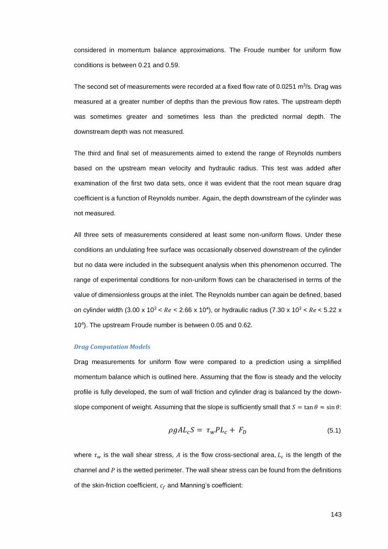
143

considered in momentum balance approximations. The Froude number for uniform flow

conditions is between 0.21 and 0.59.

The second set of measurements were recorded at a fixed flow rate of 0.0251 m3/s. Drag was

measured at a greater number of depths than the previous flow rates. The upstream depth

was sometimes greater and sometimes less than the predicted normal depth. The

downstream depth was not measured.

The third and final set of measurements aimed to extend the range of Reynolds numbers

based on the upstream mean velocity and hydraulic radius. This test was added after

examination of the first two data sets, once it was evident that the root mean square drag

coefficient is a function of Reynolds number. Again, the depth downstream of the cylinder was

not measured.

All three sets of measurements considered at least some non-uniform flows. Under these

conditions an undulating free surface was occasionally observed downstream of the cylinder

but no data were included in the subsequent analysis when this phenomenon occurred. The

range of experimental conditions for non-uniform flows can be characterised in terms of the

value of dimensionless groups at the inlet. The Reynolds number can again be defined, based

on cylinder width (3.00 x 103 < 𝑅𝑒 < 2.66 x 104), or hydraulic radius (7.30 x 103 < 𝑅𝑒 < 5.22 x

104). The upstream Froude number is between 0.05 and 0.62.

Drag Computation Models

Drag measurements for uniform flow were compared to a prediction using a simplified

momentum balance which is outlined here. Assuming that the flow is steady and the velocity

profile is fully developed, the sum of wall friction and cylinder drag is balanced by the down-

slope component of weight. Assuming that the slope is sufficiently small that 𝑆 = tan 𝜃 ≈ sin 𝜃:

𝜌𝑔𝐴𝐿𝑐𝑆 = 𝜏𝑤𝑃𝐿𝑐 + 𝐹𝐷

(5.1)

where 𝜏𝑤 is the wall shear stress, 𝐴 is the flow cross-sectional area, 𝐿𝑐 is the length of the

channel and 𝑃 is the wetted perimeter. The wall shear stress can be found from the definitions

of the skin-friction coefficient, 𝑐𝑓 and Manning’s coefficient:

144

𝜏𝑤 = 𝑐𝑓

1

2𝜌𝑈2 =

2𝑔𝑛2

𝑅ℎ1/3

1

2𝜌𝑈2 =

𝑔𝑛2

𝑅ℎ1/3 𝜌𝑈2 (5.2)

Substituting this expression for the shear stress into Eq. (5.1) gives:

𝜌𝑔𝐴𝐿𝑐𝑆 =

𝑔𝑛2

𝑅ℎ1/3 𝜌𝑈2 𝑃𝐿𝑐 + 𝐹𝐷

(5.3)

This equation can be rearranged to give a simple method of predicting the drag force from the

measured depth and flow rate:

𝐹𝐷 𝑃𝑟𝑒𝑑𝑖𝑐𝑡𝑖𝑜𝑛 = 𝜌𝑔𝐴𝐿𝑐 {𝑆 −𝑛2𝑈2

𝑅ℎ4/3

} (5.4)

The drag force is predicted under the assumption that Manning’s coefficient is equal to the

bare channel value. For comparison, three different formulations for Manning’s coefficient,

from section 4.2, have been used. Firstly, a constant value of 𝑛 = 0.0109 m-1/3s was used.

This provided the best fit over most of the range of experimental conditions in the bare channel

experiments. However, strictly speaking it is only valid for Reynolds numbers, based on

hydraulic radius, which are greater than around 30000. Many of the conditions in this

experiment fall outside this range. Secondly, Manning’s coefficient was considered to be a

function of Reynolds number, based on hydraulic radius: 𝑛 = 0.0431𝑒−8.98×10−5𝑅𝑒 + 0.00974.

This formulation gave a better fit for the bare channel experimental data over a wider range of

flows. Finally, a constant value of 0.00974 m-1/3s was used, which is valid for the bare channel

at asymptotically high Reynolds numbers.

A momentum balance was also used to model the normal depth as a function of slope and

flow rate. Equating the drag force with the previous prediction, Eq. (5.4), and substituting the

definition of the drag coefficient gives:

𝐹𝐷 = 𝜌𝑔𝐴𝐿𝑐 {𝑆 −

𝑛2𝑈2

𝑅ℎ4/3} = 𝐶𝐷

1

2𝜌𝑈2𝐷𝐻

(5.5)

Eq. (5.5) can be rearranged to find the mean velocity:

𝑆 −

𝑛2𝑈2

𝑅ℎ4/3 = 𝐶𝐷

1

2

𝜌𝑈2𝐷𝐻

𝜌𝑔𝐴𝐿𝑐=

𝐶𝐷𝑈2𝐷

2𝑔𝐵𝐿𝑐

(5.6)

𝑈2 {𝐶𝐷𝑈2𝐷

2𝑔𝐵𝐿𝑐+

𝑛2

𝑅ℎ4/3} = 𝑆

(5.7)

145

𝑈 =𝑅ℎ

2/3√𝑆

√𝑛2 +𝐶𝐷𝑅ℎ

4/3𝐷2𝑔𝐵𝐿𝑐

(5.8)

An approximation for the mean velocity can be determined with suitable approximations for 𝑛

and 𝐶𝐷. Manning’s coefficient was taken as 0.0109 m-1/3s as, of the three formulations

considered, this provided the best estimates of the drag force. This will be demonstrated later.

The drag coefficient was taken as equal to the value determined via linear regression of the

measured drag force on the dynamic pressure force for uniform flows. The volumetric flow

rate was then calculated from the continuity principle.

Finally, a model was developed for the drag force as a function of depth at a fixed flow rate

(for non-uniform flows). Substituting the continuity equation into the definition of the drag

coefficient gives:

𝐹𝐷 = 𝐶𝐷

1

2𝜌𝑈2𝐷𝐻 = 𝐶𝐷

1

2𝜌 (

𝑄

𝐵𝐻)

2

𝐷𝐻 = (𝐶𝐷 𝜌 𝑄2𝐷

2 𝐵2)

1

𝐻

(5.9)

Assuming that the drag coefficient is relatively independent of the flow conditions, if the

geometry and flow rate are fixed, it therefore follows that the drag force is inversely

proportional to the depth. Appropriate model drag coefficients, for each flow rate, were

determined via linear regression of the drag force on the reciprocal of depth. The data were

then compared to the fitted model. The purpose of this is to investigate the variation in drag

coefficient, with depth, at a fixed flow rate. It is not suggested that the drag coefficient is a

function of flow rate.


Mean Drag Coefficient at Uniform Depth

Figure 5.2 shows the measured mean drag force as a function of the dynamic pressure force.

A clear linear relationship is observed indicating that the drag coefficient is relatively

independent of Reynolds number within this range. A linear regression yields a drag coefficient

of 2.11. This value is well correlated with the experimental data with 𝑅2 > 0.99.

146

Figure 5.2 - Drag force vs. dynamic pressure force for an isolated square cylinder.

The cylinder is located at the channel centre and the depth is uniform.

Drag coefficients for studies at comparable Reynolds number are shown in Table 5.1.

Author 𝑹𝒆 𝑻𝑰 (%) 𝑫/𝑩 (%) 𝑯/𝑫 𝑪𝑫

Present study (1.0 - 2.2) x 104 ≈ 8 12.7 1.5 - 6.3 2.11

Norberg (1993) 5000 0.06 1.1 62.5 2.21

Yen and Yang (2011) 6300 0.3 4.0 25.0 1.86

Norberg (1993) 13000 0.06 1.1 62.5 2.15

Yen and Liu (2011) 21000 0.4 4.0 25.0 2.06

Lyn et al. (1995) 21400

2 7.1 9.8 2.1

Yen and Yang (2011) 24000 0.3 4.0 25.0 1.96

Yen and Yang (2011) 36000 0.3 4.0 25.0 2.02

Lee (1975) 176000 0.5 3.6 9.2 2.04

British Standards Institution (2005)

N/A N/A N/A N/A 2.1

Table 5.1 - Mean drag coefficient for isolated square cylinders from various authors.



147

There is generally reasonable agreement between the measured drag coefficients from

different laboratory studies. The maximum absolute discrepancy between values is 18.8%.

The minimum and maximum drag coefficients of 1.86 and 2.21 both occur at relatively low

Reynolds number (less than 6300). This may suggest that 𝐶𝐷 is sensitive to the value of other

parameters when Reynolds number is this low. However, all the other values agree with the

present study to within 7.1% suggesting that 𝐶𝐷 is reasonably constant for 𝑅𝑒 greater than

around 104. This is despite the fact that turbulence intensity from the various sources spans

two orders magnitude suggesting the drag coefficient is only a very weak function of

turbulence intensity. In addition, blockage ratio (𝐷/𝐵) and aspect ratio (𝐻/𝐷) appear to have

little influence on the result over a wide range of values.

With the exception of the present study and Lyn et al. (1995) the remaining experiments

summarised in Table 5.1 were conducted in wind tunnels as opposed to flumes. This would

explain why 𝑇𝐼 is much lower in these experiments as in high-quality wind tunnels 𝑇𝐼 is

typically much less than 1% (Chin 2012). The comparatively high turbulence intensity in the

present study of 8% is most likely due to the inflow conditions in the upstream pre-flume

section and the geometry of the inlet.

Drag Predictions for Uniform Flow

A momentum balance was used to estimate the drag force for a known mean velocity and

geometry (Eq. (5.4)). Estimates of the drag coefficient were then obtained via linear regression

of the drag force predictions on the dynamic pressure force. Table 5.2 shows the mean drag

coefficients computed using different values of Manning’s coefficient.

Manning’s coefficient (m-1/3/s) 𝑪𝑫 Discrepancy (%) 𝑹𝟐

N/A - strain gauge measurement 2.11 N/A 0.99

(a) 0.0109 2.32 + 10.0 0.88

(b) 0.0431e - 8.98 x 10 - 5 Re + 0.00974 1.79 - 15.2 0.50

(c) 0.0097 2.91 + 37.9 0.92

Table 5.2 - Predicted mean drag coefficients, CD for an isolated cylinder in uniform flow.

CD is computed with Eq. (5.4) using different values of Manning’s coefficient.

148

The data are reasonably well correlated for the two constant values of Manning’s coefficient,

with 𝑅2 values of 0.88 and 0.92 for 0.0109 m-1/3s and 0.0097 m-1/3s respectively. A much poorer

correlation is obtained with variable Manning’s coefficient (𝑅2 = 0.50). The closest agreement

with the measured drag coefficient was obtained when Manning’s coefficient was taken as

0.0109 m-1/3s. For the remainder of this section, drag force predictions will only use this value

of Manning’s coefficient. Figure 5.3 shows the predicted drag force as a function of the

dynamic pressure force for an isolated cylinder in the channel centre at uniform depth. The

predicted drag coefficient is 2.32, which is 10.0% higher than the measured value.

Figure 5.3 - Predicted drag vs. dynamic pressure force for an isolated square cylinder.


Figure 5.4 shows the predicted drag force against values measured directly with the strain

gauge. The solid line is a line of perfect agreement. Most of the data are above this line,

indicating that the majority of predicted values are higher than the measured values.

149

Figure 5.4 - Predicted vs. measured drag force for an isolated square cylinder.


Depth as a Function of Flow Rate for Normal Flow

Figure 5.5 shows the uniform flow depth as a function of volumetric flow rate at the three

different slopes (0.00067 (long lines), 0.00134 (medium lines), 0.00217 (short lines)). The flow

rate required for normal flow increases with an increase in depth or slope, as was observed in

the unobstructed channel. At fixed upstream depth, increasing the slope increases the down-

slope component of weight. For uniform flow this is balanced by the combined drag on the

walls and the cylinder. To achieve uniform flow the total drag must therefore increase. This

requires an increase in velocity and hence flow rate. Increases in upstream depth also result

in an increase in the down-slope component of weight. In addition, increasing the depth

reduces the velocity (at constant flow rate) with only a relatively small increase in the wetted

perimeter of the walls or the exposed frontal area of the cylinder. The combined drag force

therefore decreases. Again a larger total drag force is needed to achieve uniform flow, so

increases in velocity and hence flow rate are required.

150

Figure 5.5 - Depth vs. flow rate for uniform flow surrounding an isolated square cylinder.

The cylinder is located in the channel centre.

Dotted lines represent results from the calibrated model, Eq. (5.5). Manning’s coefficient is

taken as 0.0109 m-1/3s and the drag coefficient is taken as the measured value of 2.11. Values

determined using the model are in close agreement with those measured directly over most

of the range of conditions.

Mean Drag Coefficient at Varied Depth

This sub-section considers non-uniform flows. Figure 5.6 shows the drag force as a function

of the reciprocal of depth at various flow rates between 0.0068 m3/s and 0.0302 m3/s.

151

Figure 5.6 - Drag vs. the reciprocal of upstream depth for an isolated square cylinder.

The flow rate: (a) varies between 0.0068 m3/s and 0.0302 m3/s and (b) is fixed at 0.0251 m3/s.

(a)

(b)

152

The best fit for the drag coefficients at each flow rate are also included in Figure 5.6. The

correlation coefficients are reasonably high (0.91 < 𝑅2 < 0.99). However, a single value of the

drag coefficient tends to underestimate the drag at large depths and overestimate the drag at

small depths. The actual drag coefficient therefore decreases with increasing upstream depth.

When the downstream weir height is low, the upstream depth is much higher than downstream

depth. As the weir height is increased the flow backs up, increasing the depth along the entire

length of the channel and making it more uniform. Therefore at low upstream depths, the free-

surface level drops across the cylinder. The rear pressure force is relatively low so the drag

coefficient is relatively high. As the upstream depth increases the flow becomes more uniform

and the drag coefficient decreases.

From Figure 5.6 it also appears that a single value of the drag coefficient provides a more

reasonable fit at higher flow rates. This is due to a difference in the ratio of upstream and

downstream flow depths for the conditions tested. The maximum percentage difference

between upstream and downstream depths decreased with an increase in flow rate from

31.9% at 0.0068 m3/s to only 12.5% at 0.0302 m3/s. At higher flow rates the depth is more

uniform so the drag coefficient is less variable and closer to the typical isolated cylinder value

of 2.11.

Mean Drag Coefficient at Uniform and Non-uniform Depth

Figure 5.7 shows the drag force vs. dynamic pressure force with inclusion of all the data for

both uniform and non-uniform flows. A linear regression yields a drag coefficient of 2.26, 7.1%

higher than the value of 2.11 determined for uniform flows. The data are well correlated with

𝑅2 = 0.99 in both cases. A drag coefficient of 2.26 therefore provides good agreement over a

much wider range of flows but would typically overestimate the drag for uniform flows. The

upstream depths were much greater, or close to, the downstream depth but were never

substantially lower. The higher average drag force is to be expected as a drop in the free-

surface level is accompanied by a corresponding drop in the rear pressure force.

153

Figure 5.7 - Drag force vs. dynamic pressure force for an isolated square cylinder.

The cylinder is located at the channel centre. The depth may be uniform or non-uniform.

Root Mean Square Drag Coefficient

Figure 5.8 shows the measured root mean square drag coefficient as a function of upstream

Reynolds number, based on hydraulic radius. There is no clear difference in behaviour at

uniform depth and with a change of depth across the cylinder. Data collapse reasonably well

to a single curve. An appropriate best fit function is:

𝐶𝐷 𝑟𝑚𝑠= 18.9𝑒−2.15×10−4 𝑅𝑒 + 0.239

(5.10)

154

Figure 5.8 - RMS drag coefficient vs. Reynolds number for an isolated square cylinder.

The cylinder is located in the channel centre and the depth may be uniform or non-uniform.

Reynolds number is based on the upstream mean velocity and hydraulic radius.

Eq. (5.10) suggests that at high Reynolds number the root mean square drag coefficient is

reasonably constant with a value of approximately 0.239. This value agrees well with the value

of 0.242 obtained by Yen and Liu (2011) in a square open-loop wind tunnel at a Reynolds

number of 21000, based on cylinder width. An equivalent “hydraulic” radius, for a square wind

tunnel of side 𝐵, can be defined as the ratio of cross-sectional area to perimeter, 𝐵/4. This

gives a Reynolds number based on hydraulic radius of 1.5 x 105. This is around three times

larger than the highest Reynolds numbers considered in the present study. This suggests that

0.239 is a good approximation of 𝐶𝐷 𝑟𝑚𝑠 beyond the range considered here.

155

5.1.4 Conclusions

The isolated cylinder drag coefficient for uniform free-surface flows was found to be 2.11. This

is in close agreement with other studies over a range of Reynolds numbers between 9.5 x 103

and 1.76 x 105. This demonstrates that 𝐶𝐷 is at most a weak function of 𝑅𝑒 within this range.

Similarly, turbulence intensity spans from 0.06% to 8% with no significant influence on the

drag coefficient. The cross-sectional blockage ratio also varied markedly between studies with

values between 1.1% and 12.7% indicating that the drag coefficient is independent of

blockage ratio within this range. This suggests that in numerical simulations it may be sufficient

to use symmetry planes, as opposed to walls, for the sidewall boundary condition. In addition,

the drag coefficient is reasonably independent of aspect ratio for 1.5 < 𝐻/𝐷 < 62.5 so it may

be adequate to model the flow in numerical simulations as two-dimensional (2D).

The best prediction of the drag coefficient was obtained by assuming that Manning’s

coefficient is equal to 0.0109 m-1/2s. In this case, the predicted drag coefficient is 2.32, which

is 10.0% higher than the measured value. The predicted value relies on the assumptions that

the flow is uniform and fully developed and that Manning’s coefficient is the same as in the

unobstructed channel. If in reality the flow is not fully developed, the rate at which momentum

enters the flume test-section is lower than the rate at which it leaves. This would tend to reduce

the drag relative to the predicted value. In addition, the predicted drag coefficient is influenced

by the selection of Manning’s coefficient. Using a variable Manning’s coefficient, which is a

function of Reynolds number, underestimated the drag coefficient. The wall resistance may

have been overestimated in this case. Manning’s coefficient is perhaps lower than in the

unobstructed channel, at the same Reynolds number, due to the additional turbulence

produced in the wake of the cylinder. The value of Manning’s coefficient determined over most

of the range of bare channel conditions and the value approached at high Reynolds number

were also used. These formulations overestimated the drag coefficient by underestimating

wall resistance. A similar momentum balance approach may be more effective for cylinder

arrays where the proportional contribution of the walls of the flume to the total drag is likely to

be smaller. An accurate estimate of the drag coefficient is then less dependent on an accurate

wall drag estimate.

156

For non-uniform flows at a constant flow rate the drag coefficient decreases with increasing

upstream depth. When the downstream weir height is low, the upstream depth is much higher

than the downstream depth. The free-surface level therefore drops across the cylinder. The

rear pressure force is relatively low so the drag coefficient is relatively high. As the weir height

is increased, the depth increases and the flow becomes more uniform so the drag coefficient

decreases.

The mean drag coefficient computed using data for both uniform and non-uniform flows was

2.26. This is 7.1% higher than the value of 2.11 computed using data from uniform flows only.

The difference between the two values is large enough to suggest that, for two-cylinder tests,

it would be more appropriate to base 𝐶𝐷 only on flows which are relatively uniform. However,

the difference between the two values is small enough to suggest that small changes in

upstream depth, from the normal depth, are unlikely to substantially alter the drag coefficient.

Based on this finding, two-cylinder and array tests will primarily focus on uniform flows.

However, for a single test case, the drag force will be measured at varied depth for a number

of fixed flow rates. For this test a pair of cylinders will be separated by two cylinder widths,

between cylinder centres, in the direction of mean flow.

The root mean square drag coefficient was found to be a function of upstream Reynolds

number, based on hydraulic radius, which asymptotically approaches 0.239 at high Reynolds

number. This value agrees well with the value of 0.242 obtained by Yen and Liu (2011) at

higher Reynolds number suggesting that 0.239 is a good approximation of 𝐶𝐷 𝑟𝑚𝑠 beyond the

range considered here.

157

5.2 Isolated Cylinder Velocity Profiles

5.2.1 Aim

The aim of this short experiment was to observe how the presence of an isolated cylinder

alters the mean velocity and turbulence intensity along the channel centreline. Stream-wise

velocity profiles will be compared to that of Lyn et al. (1995).

5.2.2 Method

An isolated square cylinder of side 38 mm was placed in the centre of the flume giving a cross-

sectional blockage ratio of 𝐷/𝐵 = 12.7%. The slope was set to 0.00217. The weir height was

adjusted to achieve uniform flow. The depth was measured at several locations within the

velocity measurement region. All measurements agreed to within 1 mm. The depth was 185

mm giving an aspect ratio of 𝐻/𝐷 = 4.9. The measured mean velocity based on the flow rate

and channel cross-sectional area was 0.292 m/s. However, it is the velocity 10D upstream of

the first cylinder which has been used to normalise measured velocities. This coincides with

the location of the velocity inlet in numerical simulations so the same scaling velocity has been

used. The mean velocity, measured with the ADV, at this location was 0.295 m/s. This gives

a Reynolds number of 11100 based on cylinder width. The difference between the measured

upstream velocity in the channel centre and the cross-sectional average is only 1.0%.

Velocities were measured at 1/3 depth from the surface. This was shown to be far outside of

the boundary layer in the bare channel in section 4.3. The Reynolds number based on

hydraulic radius is comparable for the two experiments, with 24200 in this experiment

compared to 26900 for the bare channel. Velocities were measured along the lateral centreline

of the flume which passes through the centre of the cylinder. Intervals of 0.5D were used

between 5D upstream of the cylinder centre and 15D downstream. Additional measurements

were taken close to the surface of the cylinder.

The stream-wise velocity profile is also compared to that of Lyn et al. (1995). A comparison of

the flow conditions for these two experiments is shown in Table 5.3.

158

Author 𝑹𝒆 𝑻𝑰 (%) 𝑫/𝑩 (%) 𝑯/𝑫

Present study 11100 10 12.7 4.9

Lyn et al. (1995) 21400 2 7.1 9.8

Table 5.3 - Comparison of flow conditions in the present study and Lyn et al. (1995).



5.2.3 Results, Discussion and Conclusions

Stream-wise Velocity Profile

The stream-wise velocity profile in the lateral centreline of the channel is shown in Figure 5.9.

Upstream the velocity is reasonably constant but it begins to decrease rapidly towards zero at

about 3 cylinder widths upstream. The same general trends have been observed in the wake

of the cylinder in the present study and in Lyn et al. (1995). The flow separates behind the

cylinder and the velocity is negative for a short distance downstream. In the present study the

length of the separation region is close to 2.0D compared to only 1.4D in Lyn et al. (1995).

The velocity directly behind the cylinder must initially decrease from zero at the cylinder

surface towards the minimum value. In the present study the velocity 1.0D downstream is

indeed slightly higher than that 1.25D downstream. This behaviour was not observed by Lyn

et al. (1995). Further downstream the velocity begins to increase towards the upstream value.

In the present study the mean velocity initially increases rapidly reaching 80.0% of the free-

stream value by 8D downstream. The velocity then begins to increase at a slower rate

reaching 90.9% by 14.5D downstream. In the experiment by Lyn et al. (1995) the mean

velocity increases at a slower rate than in the present study. In their study the mean velocity

only reaches 62.1% of the free-stream value by 8D downstream. A wake similar to those

sketched previously in Figure 3.9 (a) and 3.13 (a) was observed.

159

Figure 5.9 - Mean velocity vs. stream-wise distance along the channel centreline.

The flow is uniform and surrounds an isolated square cylinder located at the channel centre.

Stream-wise Turbulence Intensity Profile

Figure 5.10 shows the stream-wise turbulence intensity (𝑇𝐼) profile in the lateral centreline of

the channel. At more than around two cylinder widths upstream of the cylinder 𝑇𝐼 is close to

the upstream value of 9.5%. In the wake of the cylinder 𝑇𝐼 initially increases almost linearly

reaching a peak value of 47.0% by 2.25D downstream of the cylinder centre. After reaching

the peak value over a relatively short distance, 𝑇𝐼 then begins to decay reaching 20.0% by

14.5D downstream of the cylinder centre.

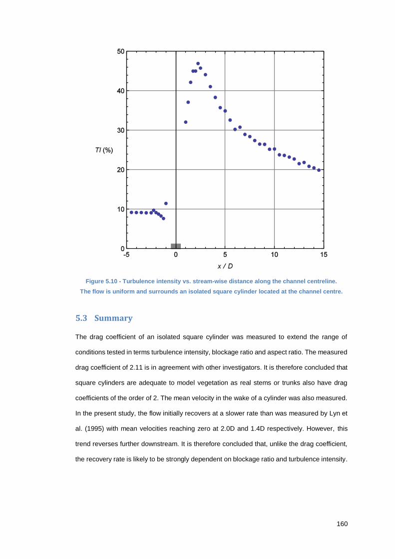
160

Figure 5.10 - Turbulence intensity vs. stream-wise distance along the channel centreline.

The flow is uniform and surrounds an isolated square cylinder located at the channel centre.

5.3 Summary

The drag coefficient of an isolated square cylinder was measured to extend the range of

conditions tested in terms turbulence intensity, blockage ratio and aspect ratio. The measured

drag coefficient of 2.11 is in agreement with other investigators. It is therefore concluded that

square cylinders are adequate to model vegetation as real stems or trunks also have drag

coefficients of the order of 2. The mean velocity in the wake of a cylinder was also measured.

In the present study, the flow initially recovers at a slower rate than was measured by Lyn et

al. (1995) with mean velocities reaching zero at 2.0D and 1.4D respectively. However, this

trend reverses further downstream. It is therefore concluded that, unlike the drag coefficient,

the recovery rate is likely to be strongly dependent on blockage ratio and turbulence intensity.

161

6 Laboratory Experiments with Cylinder Pairs

This chapter considers the laboratory experiments describing the flow around square cylinder

pairs which have been conducted as part of the present study. The main variables are the

stream-wise, 𝑠𝑥 and cross-stream, 𝑠𝑦 distance between cylinder centres. Sections 6.1 and 6.2

consider tandem cylinders where one is aligned behind the other with respect to the mean

flow (𝑠𝑦 = 0). In section 6.1 the temporally averaged drag coefficients of individual cylinders

in tandem pairs are determined as a function of their relative position. Drag coefficients are

computed as an average over a range of conditions and at fixed Reynolds number. Section

6.2 describes a short experiment in which the stream-wise velocity profiles surrounding

tandem cylinders are measured at two separation distances. The data from these experiments

are used to evaluate the validity of numerical simulations in chapter 8. The chapter concludes

with section 6.3 which considers the drag on cylinders in side-by-side (𝑠𝑦 = 0) and staggered

pairs (both 𝑠𝑥 and 𝑠𝑦 are non-zero) at constant Reynolds number. In particular, a series of

contour plots have been produced which describe the drag coefficient for cylinders in a pair at

any spacing. Cylinders of two different widths were also considered to investigate the influence

of cross-stream blockage ratio on the drag coefficient.

162

6.1 Tandem Cylinder Drag

6.1.1 Aims

Three different experiments have been conducted which measured the drag on cylinders in a

tandem pair. The aim of the first experiment was to determine the influence of upstream depth

on the downstream cylinder drag coefficient at several flow rates and a fixed separation of 2D.

The second experiment considered only cases where the depth was uniform. The main aim

of this experiment was to determine the drag coefficient of the downstream cylinder as a

function of the separation between cylinders. Mean drag coefficients were computed over a

range of flows at a fixed blockage ratio. Drag coefficients were also measured for flows with

two different blockage ratios at fixed Reynolds numbers. These flow conditions coincide with

the conditions in experiments with staggered cylinder pairs, which are considered later. The

results with different flow conditions are compared. The secondary aim of this experiment is

therefore to investigate the influence of blockage ratio and Reynolds number in determining

the drag coefficient in downstream cylinder pairs. The results from this experiment were used

to select appropriate separation distances for two test cases. For these test cases stream-

wise velocity profiles, along the centreline of the cylinders, were also measured in a later

experiment. Measured drag coefficients and velocity profiles were used to evaluate the validity

of the realizable k-epsilon (𝑘-휀) turbulence model for the prediction of flow surrounding tandem

cylinders.

The aim of the third and final (short) experiment was to determine the mean upstream cylinder

drag coefficient for a separation of 3D. The mean drag was determined over a range of

conditions with uniform depth. It was assumed that the drag coefficient of the upstream

cylinder drag will tend to the isolated cylinder value with respect to separation distance at a

much faster rate than the downstream cylinder. The drag coefficient with a separation of 3D

was therefore compared to the isolated cylinder value to see if there was a significant

difference.

163

6.1.2 Method

In all three experiments the drag was measured on a cylinder with a fixed position in the centre

of the flume and the other cylinder was moved to create the correct relative position. The drag

on a single cylinder was measured under various flow conditions with channel slopes of

0.00067, 0.00134 and 0.00217.

In the first experiment, the drag was measured on the downstream cylinder in a tandem pair

separated by 2D. Measurements were taken at various upstream depths between 61 mm and

237 mm at four fixed flow rates between 0.0067 m3/s and 0.0260 m3/s. Depending on the flow

rate and weir height, the free-surface level may have been relatively constant or there may

have been a significant drop across the cylinders. Schematics of these setups are shown in

Figure 6.3 (a) and (b) respectively. The Reynolds number is between 8600 and 44300 based

on hydraulic radius and between 3500 and 23000 based on cylinder width.

Figure 6.1 - Schematic sketches of the free-surface level close to a pair of cylinders.

Across the cylinders the free-surface level: (a) is uniform and (b) drops significantly.

In the second experiment the drag on a downstream cylinder was measured at variable

stream-wise separation. Measurements were taken at various upstream depths between 104

mm and 238 mm and at flow rates between 0.0087 m3/s and 0.0239 m3/s. The weir height

was adjusted such that there was no observable drop in the free-surface level across the

cylinders (Figure 6.1 (a)). It would perhaps have been better to specify a percentage within

which depth measurements agreed. This would have been rather time consuming as a large

number of drag measurements were taken. The fact that the definition of conditions with no

observable drop in the free-surface level is subjective is not a major concern. This is because

the drag coefficient was found to be fairly constant with respect to flow conditions. This is

𝑈 𝑈

(a) (b)

164

demonstrated later. At each slope and flow rate the drag was measured at two depths. The

first depth was achieved by slowly increasing the weir height until the flow backed up to the

location of the upstream cylinder. The second depth was larger than this. When the depth was

increased slightly the depths upstream and downstream were still reasonably close. If the weir

height had been lowered the variation in depth with stream-wise distance would be significant.

The Reynolds number is between 11400 and 35400 based on hydraulic radius and between

4800 and 16500 based on cylinder width. The upstream Froude numbers are always less than

one. The mean drag coefficient for each separation was found via linear regression of the drag

force on the dynamic pressure force. For consistency, the drag coefficient of an isolated

cylinder was re-measured under the same conditions. A value of 2.03 was obtained, which is

just 3.8% lower than the value of 2.11 obtained over a range of normal flow conditions, in

section 5.1.

Additional measurements of the drag on a cylinder as a function of stream-wise separation

between tandem pairs were also taken as part of the second experiment. These additional

measurements were taken under the same conditions as experiments with cylinders in side-

by-side and staggered cylinder pair tests. These tests are considered later in section 6.3. The

measurements were conducted with pairs of square cylinders of side 16 mm or 38 mm giving

cross-stream blockage ratios, 𝐷/𝐵 of 6.3% and 12.7% respectively. Velocities for the two

blockage ratios (two different cylinder widths) were comparable so the Reynolds number

based on cylinder width also differs. The Reynolds number based on cylinder diameter is 7540

at 6.3% blockage and 16000 at 12.7% blockage. Ideally experiments with staggered arrays

for the two blockage ratios would have been tested at the same Reynolds number. However,

it was also desirable to conduct tests at high Reynolds number so that results can be

extrapolated beyond the range considered here. Yen and Liu (2011) showed that for side-by-

side cylinders 𝐶𝐷 is independent of Reynolds number for 𝑅𝑒 > 17000. The Reynolds number

at 12.7% blockage is only 5.9% lower than this value suggesting these results can be

extrapolated to higher Reynolds number. However, at the lower blockage ratio (with the

thinner cylinders) it was not possible to obtain uniform flow at such high velocities. It was

therefore decided to conduct the two tests at Reynolds numbers towards the high end of what

was possible with the available equipment rather than the same lower value. In section 5.1 it

165

was demonstrated that the drag coefficient is reasonably independent of blockage ratio for

blockage ratios as high as 12.7%. However, the influence of blockage ratio is anticipated to

be more pronounced when there is an offset between cylinders in the cross-stream direction.

This is because the effective cross-sectional blockage ratio of two side-by-side cylinders is

double that of an isolated cylinder or two cylinders in tandem. The two blockage ratios are

compared in this section to investigate the effects of Reynolds number with cylinders in

tandem where the flow is less sensitive to blockage ratio. Further details about the

experimental method such as other inflow conditions, cylinder positions and the degree of flow

uniformity are given in section 6.2.2.

In the third and final (short) experiment the drag was measured on the upstream cylinder in a

tandem pair separated by 3D. The free-surface level was relatively constant. Measurements

were taken at various upstream depths between 125 mm and 224 mm and at flow rates

between 0.0102 m3/s and 0.0226 m3/s. The Reynolds number is between 14500 and 31300

based on hydraulic radius and between 6400 and 13600 based on cylinder width.

6.1.3 Results Discussion and Conclusions

Downstream Cylinder Drag Force at Variable Upstream Depth

Figure 6.2 shows the drag force on the downstream cylinder as a function of the dynamic

pressure force at a fixed separation, 𝑠𝑥 = 2D. For a given flow rate, at large upstream depths

(smaller dynamic pressure forces) the flow reattaches on the downstream cylinder giving

negative drag. This occurs when there is a negligible drop in the free surface across the

cylinders. Under these conditions the drag coefficient is reasonably constant. Linear

regression of the drag force on the dynamic pressure force taking into account only the

conditions where the flow is relatively uniform gives a value of -0.45. As the depth is reduced

(dynamic pressure force is increased) there is a significant drop in the free-surface elevation

across the cylinders so the rear pressure force decreases and the drag coefficient increases.

166

Figure 6.2 - Drag vs. dynamic pressure force for the downstream cylinder.

The cylinders are in tandem and separated by sx = 2D between centres.

Drag Force for Uniform Flow at Variable Separation

Figure 6.3 shows the drag force on the downstream cylinder as a function of the dynamic

pressure force at various spacing ratios. At fixed separation there is a clear linear relationship

between the drag force and dynamic pressure force. The data are well correlated with 𝑅2 =

0.958 and 𝑅2 = 0.970 for 𝑠𝑥 = 2D and 𝑠𝑥 = 3D respectively with 𝑅2 > 0.996 elsewhere. This

suggests that drag coefficient is a strong function of positioning and is relatively independent

of the flow under these conditions. It is also clear that the drag coefficient increases with

downstream distance.

167

Figure 6.3 - Drag vs. dynamic pressure force for the downstream cylinder (2).

The cylinders are in tandem with various x-separation distances between centres, sx.

Figure 6.4 shows the downstream cylinder drag coefficient as a function of spacing ratio with

no substantial drop in the free surface across the cylinders. When cylinder pairs are in tandem,

the downstream cylinder is shielded from the fast-moving flow so the drag coefficient is

consistently less than the isolated cylinder value of 2.11. When cylinders are sufficiently close

(𝑠𝑥/𝐷 = 2) the flow separates behind the upstream cylinder and reattaches on the downstream

one, so 𝐶𝐷 is negative. As cylinders are moved further apart shielding is reduced so 𝐶𝐷

increases. At relatively close spacing (𝑠𝑥/𝐷 ≤ 4) the drag coefficient is very sensitive to

position. As the separation increases further, the drag coefficient increases much more slowly

approaching the isolated cylinder value at large cylinder separations.

168

Figure 6.4 - Flow-averaged drag coefficient vs. stream-wise separation between centres

for the downstream cylinder in a tandem pair.

Figure 6.5 shows the measured drag coefficients as a function of stream-wise separation at

two different combinations of blockage ratio and Reynolds number. The flow-averaged values,

previously shown in Figure 6.4, have also been included for comparison. Despite

discrepancies in the values between each data series, the same general trend is observed.

The drag increases from a negative value when the cylinders are relatively close, towards the

isolated cylinder value as separation increases. For consistency the isolated cylinder drag was

re-measured for the same combinations of blockage ratio and Reynolds number. At 12.7%

blockage the measured drag coefficient is 2.06, which is only 2.4% lower than flow averaged

value. However, at 6.3% blockage the measured value is 1.79, 15.2% lower than the flow

averaged value. This difference is significant suggesting that Reynolds number does have a

significant impact on 𝐶𝐷 when 𝑅𝑒 is this low.

Isolated cylinder drag coefficient, CD = 2.11

169

Figure 6.5 - Drag coefficient vs. stream-wise separation between centres

for the downstream cylinder in a tandem pair.

Downstream cylinder drag measurements have been the main focus so far. This is because

the upstream cylinder drag coefficient is expected to be a weaker function of separation than

the downstream cylinder. It has been shown that an upstream cylinder can shield downstream

cylinders from high velocity flow resulting in substantial reduction in the downstream cylinder

drag coefficient. This effect is expected to be far more pronounced than the change in the

drag coefficient of an upstream cylinder due to the positioning of a cylinder downstream. This

was observed previously with circular cylinders by Liu et al. (2008). However, it is often the

average drag across two cylinders which is of interest so the drag coefficient of the upstream

cylinder also needs to be measured.

170

Figure 6.6 shows the drag force on an upstream cylinder as a function of the dynamic pressure

force for a tandem pair separated by 𝑠𝑥 = 3D. Linear regression yields a drag coefficient of

2.21, 4.7% higher than the value obtained for an isolated cylinder at uniform depth. These

values are relatively close suggesting that the drag coefficient of a cylinder more than 3D

upstream is also likely to be close to the isolated cylinder value. For future experiments with

staggered cylinders the drag will be measured for 5 cylinder widths upstream.

Figure 6.6 - Drag force vs. dynamic pressure force for an upstream cylinder.

The cylinders are in tandem and separated by sx = 3D between centres.

171

Test Cases for Numerical Simulations

Based on the results in this section, separation distances of 2.5D and 10D between the

cylinder centres will be used as test cases to evaluate the validity of the realizable k-epsilon

(𝑘-휀) turbulence model for predicting the flow surrounding tandem cylinders. The drag

coefficients determined at these separations are shown in Table 6.1. 𝐶𝐷 was not measured at

a spacing of 2.5D so it was estimated as the average of values at spacings at 2D and 3D. This

seems reasonable as 𝐶𝐷 increases almost linearly with 𝑠𝑥 in this range (see Figure 6.5).

𝑫/𝑩 (%) 𝑹𝒆 𝑪𝑫 (𝒔𝒙 = 𝟐. 𝟓𝑫) 𝑪𝑫 (𝒔𝒙 = 𝟏𝟎𝑫)

12.7 16000 0.04 1.43

12.7 4800 - 16500 0.06 1.59

6.3 7540 0.13 1.35

Table 6.1 - Measured drag coefficients at separations of sx = 2.5D and sx = 10D.

Separations of 2.5D and 10D were chosen for two main reasons. Firstly, the downstream

cylinder drag coefficients measured at constant Reynolds number were in closer agreement

with the flow-averaged values than at some other separation distances. This suggests that at

these spacings the drag coefficient is less sensitive to blockage ratio or Reynolds number.

Secondly, the drag coefficient differs substantially for the two cases so the flow behaviour is

also expected to differ substantially. With 2.5D separation the drag is negligible compared to

the isolated value so it is expected that the flow will recover very little downstream of the first

cylinder. With 10D separation the drag is much larger than zero but still significantly less than

the isolated cylinder value so it is expected that the flow will recover to some degree. The

Reynolds number for numerical simulations is of the order of 16000. At this Reynolds number

the measured downstream cylinder drag coefficient is 0.04 for 2.5D separation and 1.43 for

10D separation. In either case the upsteam cylinder drag coefficient is expected to be close

to the free-stream value of around 2.11. Stream-wise velocity profiles along the centreline of

a tandem cylinder pair were also measured under the same conditions in the next experiment

described.

172

6.2 Tandem Cylinder Velocity Profiles

6.2.1 Aims

The main aim of this short experiment was to observe the influence of the separation distance

between tandem cylinders on the stream-wise velocity profiles along the channel centreline.

This will be achieved by comparing velocity profiles for two test cases with cylinder separations

of 2.5D and 10D. Velocity profiles will be used later to evaluate the validity of the realizable k-

epsilon (𝑘-휀) turbulence model for the use of predicting the flow around tandem cylinders. The

secondary aim of this experiment was to observe the influence of the separation distance on

turbulence intensity.

6.2.2 Method

The upstream cylinder was placed in the centre of the flume. The downstream cylinder was

then placed the desired distance downstream. The slope was set to the lowest value of

0.00067. The upstream depth was 127 mm giving an aspect ratio of 𝐻/𝐷 = 3.3. The measured

mean velocity based on the flow rate and channel cross-sectional area was 0.419 m/s.

However, it is the velocity 10D upstream of the first cylinder which has been used to normalise

measured velocities. This coincides with the location of the velocity inlet in numerical

simulations so the same scaling velocity has been used. The mean velocity, measured with

the ADV, at this location was 0.424 m/s. This gives a Reynolds number, based on cylinder

width, of 16100. The difference between the measured upstream velocity in the channel centre

and the cross-sectional average is only 1.2%. The flow conditions specified above are for the

test case with 2.5D separation between cylinder centres. The difference in upstream depth

and velocity between the two test cases is less than 0.8%.

173

It was not possible to achieve a completely uniform flow for both test cases at the same

Reynolds number and aspect ratio. A reasonable approximation was achieved with no

significant change in the free-surface level across the cylinders. The depth was measured at

several locations along the region in which velocities were measured. The maximum

difference between depth measurements at various locations was 3.9% which is small in

relation to the overall depth.

Velocities were measured at 1/3 upstream depth from the surface which was shown to be far

outside of the boundary layer in the bare channel experiments in section 4.3. The Reynolds

number based on hydraulic radius is comparable for the two experiments with 28000 in this

experiment compared to 26900 for the bare channel. Velocities were measured along the

lateral centreline of the flume which passes through the centre of the cylinders. Intervals of

0.5D were used between 5D upstream of the first cylinder and 15D downstream of the second.

Additional measurements were taken close to the surface of the cylinders.

6.2.3 Results, Discussion and Conclusions

Stream-wise Velocity Profiles

Stream-wise velocity profiles of tandem cylinders separated by a distance of 2.5D and 10D

are shown in Figure 6.7. At both separations, the velocity 5D upstream of the first cylinder is

close to the upstream value used for normalisation (10D upstream). The velocity then begins

to decrease rapidly about 3 cylinder widths upstream of the first cylinder. This behaviour is

similar to the flow upstream of an isolated cylinder. With the cylinders sufficiently close (𝑠𝑥 =

2.5D) all velocity measurements between the two cylinders are negative. The velocity must

increase towards zero at the downstream cylinder surface but this behaviour is confined to a

very narrow region. When the cylinders are further apart the velocity recovers significantly

behind the first cylinder. At 𝑠𝑥 = 10D the velocity between the cylinders reaches about 70% of

the free-stream value. The velocity then reduces towards zero at the downstream cylinder

surface. Downstream of the second cylinder the flow behaviour is again similar at both cylinder

separations. Measured velocities are negative for about 1.5 cylinder widths from the cylinder

centre. The flow then recovers with a negligible difference from the free-stream value a further

15D downstream.

174

Figure 6.7 - Mean velocity vs. stream-wise distance for tandem cylinders.

The cylinders are separated by: (a) 2.5D and (b) 10D between centres.

(a)

(b)

175

Similar flow structures to those sketched previously in Figure 3.12 (b) and (c) were observed

respectively at 2.5D and 10D separation.

An estimate of the drag force on the downstream cylinders can be obtained from the typical

isolated cylinder drag coefficient if an appropriate velocity scale is used in place of the mean.

At 2.5D separation the drag is negligible. At 10D separation, taking 𝐶𝐷 = 2.11 and the velocity

scale as 𝑈 overestimates the drag force (measured in section 6.1.3) by 47.6%. If however, the

peak velocity between the cylinders is used in place of 𝑈 the approximation improves and the

drag is underestimated by 27.7%. This estimate is clearly crude but could still be useful in the

field to estimate the forces on sparsely arranged vegetation or other obstacles. This is

beneficial as drag force measurements are more difficult to obtain in the field than velocity

measurements.

Turbulence Intensity Profiles

Figure 6.8 shows turbulence intensity, 𝑇𝐼 as a function of stream-wise distance for tandem

cylinders separated by 2.5D and 10D. At both separations 𝑇𝐼 upstream of the first cylinder is

around 8%. In the wake of the upstream cylinder 𝑇𝐼 initially increases almost linearly towards

a peak value. When the cylinders are sufficiently close (𝑠𝑥 = 2.5D) 𝑇𝐼 increases over the entire

measured range but when the cylinders are further apart (𝑠𝑥 = 10D) it reaches its peak value

after a relatively short distance and then begins to decay. Trends in turbulence intensity in the

wake of the downstream cylinder are similar for the two separations. This qualitative behaviour

is also similar to that observed in the wake of the upstream cylinder when the cylinders are

separated by 10D. 𝑇𝐼 increases almost linearly, over a short distance, reaches a peak value

and then decays exponentially reaching 16% by 15D downstream of the second cylinder. At

both cylinder separations the peak between cylinders is slightly higher than the downstream

peak. Peak values are similar for the two cylinder separations.

176

Figure 6.8 - Turbulence intensity vs. stream-wise distance for tandem cylinders.

The cylinders are separated by: (a) 2.5D and (b) 10D between centres.

(a) (b)

177

6.3 Two Cylinder Drag in Side-by-Side and Staggered Arrangements

6.3.1 Aims

Two experiments were conducted with pairs of cylinders in side-by-side and staggered

arrangements. The aim of the first experiment (symmetry test) was to compare measured drag

coefficients, for a cylinder in the centre of the channel, in two symmetric side-by-side

configurations. This is to check the assumption that, due to symmetry, the drag coefficients

for the two cases will be equal. The aim of the second experiment (side-by-side and staggered

cylinder pair drag) was to determine the drag coefficient of the downstream cylinder as a

function of stream-wise and cross-stream separation. Cylinder pairs will be in various side-by-

side and staggered arrangements and trends at two blockage ratios will be compared.

6.3.2 Method

Symmetry Test

The first experiment was conducted with a pair of square cylinders of side 38 mm giving a

cross-stream blockage ratio, 𝐷/𝐵 = 0.127. The slope was set to a fixed value 0.00067. A

schematic sketch of cylinder positions for the symmetry test is shown in Figure 6.9.

Figure 6.9 - Schematic sketch of cylinder positions for the symmetry test.

One cylinder is in the channel centre (dark grey) and the other (light grey) is placed at y = ±2D.

Mean flow

178

The drag on a cylinder in the centre of the flume (𝑦 = 0) was measured directly with the strain

gauge. The other cylinder was placed such that the two cylinders were separated by a distance

of 2D in the cross-stream direction. This was repeated for a range of flows with 𝑦 = ±2D. The

weir height was raised until the flow backed up to the location of the cylinders. The depth was

not completely uniform but there was no significant drop in the free-surface level downstream

of the cylinders. The upstream depth varied between 152 mm and 233 mm giving cylinder

aspect ratios, 𝐻/𝐷 between 4.0 and 6.1. Mean velocities were within the range of 0.148 m/s

< 𝑈 < 0.337 m/s. This gives Reynolds numbers between 5600 and 12800 based on cylinder

width or between 13300 and 30900 based on the upstream hydraulic radius i.e. neglecting the

presence of the cylinders.

Side-by-Side and Staggered Cylinder Pair Drag Setup

Side-by-side and staggered cylinder pair tests were conducted with pairs of square cylinders

of side 16 mm and 38 mm giving cross-stream blockage ratios, 𝐷/𝐵 of 6.3% and 12.7%

respectively. In section 5.1 it was demonstrated that the drag coefficient is reasonably

independent of blockage ratio for blockage ratios as high as 12.7%. However, the influence of

blockage ratio is anticipated to be more pronounced when there is an offset between cylinders

in the cross-stream direction. This is because the effective cross-sectional blockage ratio of

two side-by-side cylinders is double that of an isolated cylinder or two cylinders in tandem.

The drag was measured directly on a single cylinder with a fixed position in the centre of the

flume and the other block was moved around it to give the correct relative positioning as shown

in Figure 6.10. The strain gauge position was fixed for a number of reasons. Firstly, moving

the strain gauge frequently in test runs tended to alter the calibration slightly. Secondly,

moving it each time would have been time consuming. Thirdly, the current equipment setup

only allows measurements at a few cross-stream locations. Keeping the test cylinder in a fixed

position also eliminates potential variations in the drag coefficient due to its position relative

to the wall. However, the distance between the other cylinder and the wall varies with stream-

wise separation. The second cylinder was moved to each stream-wise location in turn at a

constant cross-stream separation. The process was then repeated for each cross-stream

separation. The same data have been plotted for cylinders in tandem as in section 6.1.

179

Measurements were taken on several different occasions but differences in the flow rate were

negligible with a maximum discrepancy of 0.8% between values.

Figure 6.10 - Schematic sketch of the staggered cylinder pair setup.

One cylinder is in the channel centre (dark grey) and the other (light grey) is moved around it.

The slope was fixed at 0.00067. The weir height was raised until the flow backed up to the

location of the cylinders when they were separated by 5D in the stream-wise direction. The

depth was not completely uniform but there was no significant drop in the free-surface level

downstream of the cylinders. The weir height was then fixed at this position. The upstream

depth tended to decrease slightly as the rear cylinder was moved further downstream. The

nominal upstream depth was 146 mm at 6.3% blockage and 127 mm at 12.7% blockage. The

maximum discrepancy between these values and the measured upstream depths was 4.8%.

Stream-wise separations span between 5D upstream and 20D downstream. Cross-stream

separations span between 0 (tandem) and 3.5D for 12.7% blockage and between 0 and 7D

for 6.3% blockage. Drag was recorded at various stream-wise and cross-stream separations.

Separation intervals were increased from 0.5D, when the cylinders were relatively close, to

2D when the cylinders were separated by a relatively large distance. The size of the intervals

increases with distance because it was anticipated that the drag coefficient would be a weaker

function of position at larger cylinder separations.

𝑠𝑦

𝐵/2

𝐷/2

𝑠𝑥

Mean flow

180

Velocities for the two blockage ratios (two different cylinder widths) were comparable so the

Reynolds number based on cylinder width also differs between the two test cases. The

Reynolds number is 7540 at 6.3% blockage and 16000 at 12.7% blockage. Yen and Liu (2011)

showed that for side-by-side cylinders 𝐶𝐷 initially increases with 𝑅𝑒 but is independent of

Reynolds number for 𝑅𝑒 > 17000. The Reynolds number at 12.7% blockage is only 5.9% lower

than this value suggesting these results can be extrapolated to higher Reynolds number.

Ideally the two blockage ratios would have been tested at the same Reynolds number.

However, it was also desirable to conduct tests at high Reynolds number so that the trends

extend beyond the Reynolds number considered. This also means that the results are

applicable to practical applications with fully turbulent flow. Ideally then both blockage ratios

would be tested at the higher Reynolds number. With the thinner cylinders however, it was

not possible to obtain uniform flow at high enough velocity. It was therefore decided to conduct

the two tests at Reynolds numbers towards the high end of what was possible with the

available equipment rather than at the same lower value.

For consistency the isolated cylinder drag was re-measured under the same conditions as this

experiment. At 12.7% blockage the measured drag coefficient is 2.06, which is only 2.4%

lower than flow averaged value. However, at 6.3% blockage the measured value is 1.79,

15.2% lower than the flow averaged value. This difference is significant suggesting that

Reynolds number does have a significant impact on 𝐶𝐷 at such a low Reynolds number. This

makes comparisons between the two blockages more difficult but it is still possible to comment

on the relative magnitude of the drag in relation to the measured isolated cylinder value for

those conditions.

Side-by-Side and Staggered Cylinder Pair Drag Data Analysis

The mean drag coefficient of a cylinder pair was computed as the average of the upstream

and downstream cylinder measurements at the same relative spacing. For a stream-wise

separation of 5D or less, the drag was measured on both the upstream and downstream

cylinders. For an 𝑥-separation greater than 5D, the drag was only measured on the

downstream cylinder and the drag coefficient of the upstream cylinder was assumed to be

equal to the isolated cylinder value. This assumption seems reasonable as it was shown in

181

section 6.1 that the drag coefficient of an upstream cylinder in a tandem pair at 12.7%

blockage is within 4.7% of the isolated cylinder value when the separation between centres is

just 3D. It will be shown later that, at the same blockage ratio, the upstream cylinder drag

coefficient is consistently close to the isolated cylinder value for a stream-wise separation of

5D. At 6.3% blockage however, the upstream cylinder drag coefficient is higher than the

isolated cylinder value at 5D separation. The assumption that the upstream cylinder drag is

equal to the isolated cylinder value for separations greater than 5D is therefore inaccurate at

this blockage ratio.

The drag was always measured on the centremost cylinder as shown in Figure 6.11. This

means that when measuring the drag on the upstream cylinder, the downstream cylinder is

closer to the wall (Figure 6.11(a)). However, when measuring the drag on the downstream

cylinder, at the same relative spacing, it is the upstream cylinder which is closer to the wall

(Figure 6.11(b)). It is worth noting therefore that the computed mean drag across a cylinder

pair is not necessarily the same as the mean drag on pairs with either configuration. In fact, if

the flow is diverted away from the walls the drag coefficient based on measurements with the

cylinder in the centre is likely to be higher.

Figure 6.11 - Schematic sketch of the staggered cylinder pair setup (2).

Drag is measured on the central cylinder (dark grey) when the other cylinder (light grey)

is placed: (a) downstream and (b) upstream.

(a) (b) Mean Mean flow flow

182

The strain gauge setup does not allow measurements with the cylinders very close together.

The force balance is suspended from a frame which sits above the flume. Four bars extend

downwards from the force balance and are attached to the top of the cylinder via a base plate.

This plate prevents cylinder separations of less than around 1.5D. Later, contour plots show

𝐶𝐷 as a function of 𝑠𝑥/𝐷 and 𝑠𝑦/𝐷 (Figure 6.15 and Figure 6.17). From these plots the drag

coefficient can be estimated for any relative separation, within the measured region. It is

desirable for these plots to show estimates of the drag coefficient when the cylinders are close.

Additional assumptions are therefore needed to plot trends when the cylinders are closer

together than it was practical to measure here. For touching tandem cylinders the upstream

cylinder drag coefficient was assumed to be equal to the isolated cylinder value. The

downstream cylinder drag coefficient was then selected to give the same mean drag

coefficient for the cylinder pair as the known value of a rectangular cylinder with an aspect

ratio, 𝑑/𝐷 (the ratio of stream-wise to cross-stream cylinder dimensions) of 2. For two touching

side-by-side cylinders the drag coefficients were assumed to be equal. The drag coefficient

was therefore taken as the known value of a rectangular cylinder with an aspect ratio of 0.5.

These are only approximations so it is necessary to be sceptical of drag coefficients when

both 𝑠𝑥 and 𝑠𝑦 are less than 1.5D. It is also necessary to be sceptical of the mean drag

coefficient across a pair of cylinders for stream-wise cylinder separations larger than 5D.

Known values for rectangular cylinders with aspect ratios of 0.5, 1.0 and 2.0 are shown in

Table 6.2. For side-by-side cylinders values from the British Standards Institution (2005) also

agree with Yen and Liu (2011).

Cylinder arrangement 𝒅/𝑫 𝑪𝑫 Author

Isolated (D/B = 12.7%) 1.0 2.11 Present study

Isolated (D/B = 6.3%) 1.0 1.79 Present study

Tandem (sx = 1) 2.0 1.65 British Standards Institution (2005)

Side-by-side (sy = 1) 0.5 2.24 Yen and Liu (2011)

Table 6.2 - Mean drag coefficients for rectangular cylinders from various authors.

d/D is the ratio of the stream-wise to cross-stream cylinder dimensions.

183

At 12.7% blockage the isolated cylinder drag coefficient was taken as 2.11 as determined over

a range of normal flow conditions in section 5.1. The value measured under the same flow

conditions as this experiment is 2.06. The difference between these two values is negligible

at 2.4%. However, at 6.3% blockage the measured value is 1.79, which is 15.2% lower than

the flow averaged value at higher blockage. In addition, it was anticipated that the drag

coefficient of a downstream cylinder in a tandem pair would be lower than the isolated cylinder

value. Initial inspection of the data showed that the downstream cylinder drag is consistently

lower than 1.79 at 6.3% blockage. At this blockage ratio the isolated cylinder drag is therefore

taken as 1.79.


Symmetry Test

Figure 6.12 shows the drag force on a cylinder, in a side-by-side pair separated by 𝑠𝑦 = ±2D,

as a function of dynamic pressure force. All points conform reasonably well to a single straight

line with 𝐶𝐷 = 3.36. If instead, the drag coefficient is obtained by a separate linear regression

on each data series the difference is negligible at only 2.1%. This suggests that the flow is

almost symmetric with respect to the 𝑦-axis as expected. Therefore, it is unimportant which

side of the flume (positive or negative 𝑦) the second cylinder is placed on.

184

Figure 6.12 - Side-by-side cylinder symmetry test: drag force vs. dynamic pressure force.

Drag is measured on the centre cylinder (y = 0). The other cylinder is placed at y = ±2D.

Side-By-Side Cylinder Pair Drag

Drag coefficients for side-by-side cylinders are shown in Figure 6.13. The drag coefficient is a

weak function of 𝑦-separation providing that the separation is sufficiently small (𝑠𝑦 ≤ 4D). 𝐶𝐷

is instead controlled by blockage ratio and perhaps also Reynolds number. The measured

drag coefficient is consistently higher at the larger blockage ratio of 12.7%. This is to be

expected as a larger increase in velocity, outside of the cylinder wake, is required to satisfy

the continuity principle, resulting in a larger pressure drop. However, the drag coefficient could

also be influenced by the difference in Reynolds number which is significantly lower for 6.3%

blockage. At both blockages, 𝐶𝐷 is roughly 50% higher than the isolated cylinder value

measured under the same conditions. This is in contrast to the work of Yen and Liu (2011)

who found that the drag coefficient is consistently less than the isolated cylinder value at a

Reynolds number of 21000 and a lower blockage ratio of 4%. The exception to this is when

the cylinders were sufficiently close that no flow could develop in the gap between them. This

only occurs when 𝑦 is much smaller than was considered here. Yen and Liu (2011) showed

185

𝐶𝐷 was independent of 𝑅𝑒 for side-by-side cylinders at Reynolds numbers greater than 17000.

The Reynolds number at 12.7% blockage is only 5.9% lower than this value. It is therefore

expected that this difference in behaviour is due primarily to blockage ratio as well as

differences in the experiment setup as opposed to Reynolds number. Whilst the blockage ratio

has been shown to be unimportant at 12.7% for isolated cylinders it is of higher importance in

side-by-side and near side-by-side configurations as twice the effective fraction of the cross-

section is blocked. This explains why the drag coefficient for side-by-side cylinders

consistently increases with an increase in blockage ratio. In addition, in Yen and Liu’s (2011)

experiment no cylinder position is fixed and the centreline of the flume instead passes through

the middle of the two cylinders. In contrast, in this experiment the drag is measured on the

centremost cylinder. As it would be anticipated that the velocities are higher close to the

channel centre this positioning would also tend to increase the drag coefficient.

Figure 6.13 - Drag coefficient vs. separation between centres for side-by-side cylinders.

186

At 6.3% blockage, after the initially constant region, 𝐶𝐷 decreases abruptly towards the

isolated cylinder value. As the cylinders are separated further, one cylinder is placed closer to

the flume wall so the flow is diverted towards the test cylinder and 𝐶𝐷 increases.

The flow patterns observed during this experiment were similar to those sketched previously

in Figure 3.13 to some extent but differences did occur due to the wall position and lack of

symmetry.

Staggered Cylinder Pair Drag

This sub-section now considers the general case of staggered cylinder pairs in which both the

stream-wise and cross-stream separation are variable. Figure 6.14 shows the downstream

cylinder drag coefficient (negative 𝑠𝑥 indicates the cylinder is upstream) as a function of

stream-wise separation at various cross-stream separations. Plots (a) and (b) show results at

blockage ratios of 6.3% and 12.7% respectively. The same data are represented as a contour

plot in Figure 6.15. The position of one cylinder is shown with its centre at the origin. Contours

show the drag coefficient of the other cylinder as a function of the stream-wise and cross-

stream separation between the cylinders (normalised by the cylinder width). Positive values

of 𝑠𝑥 indicate that the second cylinder is downstream of the one at the origin. Again, plots (a)

and (b) show results at blockage ratios of 6.3% and 12.7% respectively.

187

Figure 6.14 - Drag coefficient vs. stream-wise separation at various y-separations, sy.

Positive sx indicates that drag is measured on the downstream cylinder.

The blockage ratio is: (a) 6.3% and (b) 12.7%.

(a) (b)

Figure 6.15 - Drag coefficient contours as a function of cylinder separation.

One cylinder is located at the origin. Contours show the drag coefficient of the other cylinder.

Positive sx indicates this cylinder is downstream. The blockage ratio is: (a) 6.3% and (b) 12.7%.

(a)

𝑈

(b)

𝑈

18

8

189

When tandem cylinders (𝑠𝑦 = 0) are sufficiently close (𝑠𝑥/𝐷 ≤ 2), the flow separates behind

the upstream cylinder and reattaches on the downstream one, so 𝐶𝐷 is negative. As the

cylinders are moved further apart shielding is reduced and the drag coefficient increases with

downstream distance. At relatively close spacing the drag coefficient is very sensitive to

position but it increases much more slowly towards the isolated cylinder value at distances far

from the cylinder.

With small 𝑦-separation (0.5D) 𝐶𝐷 is larger than in tandem pairs for small 𝑠𝑥 but close to the

tandem value when 𝑠𝑥 is large. This is because the cylinders are no longer one behind the

other with respect to the mean flow direction so shielding is reduced. The measured drag is

consistently positive even at 1.5D between cylinder centres so the flow does not reattach on

the downstream block. For intermediate values of 𝑠𝑦 the downstream drag increases

substantially as the 𝑥-separation approaches zero. This is due to the increase in the fractional

coverage of the cross-section when the cylinders are side-by-side. For this reason, at the

higher blockage of ratio 12.7%, the peak drag for any given 𝑠𝑦 consistently occurs with the

cylinders close to side-by-side.

At high blockage (𝐷/𝐵 = 12.7%), 𝐶𝐷 typically increases with increasing 𝑦 and may be higher

or lower than the isolated cylinder value. If 𝑠𝑦 is small the upstream cylinder still shields the

downstream cylinder from the fast-moving flow to some extent. The downstream cylinder drag

coefficient is therefore less than the isolated cylinder value of 2.11. As 𝑦 increases, shielding

is reduced and the drag coefficient increases. At sufficiently large 𝑠𝑦 the second cylinder is

close to the wall so flow is diverted towards the test cylinder and the drag coefficient increases

above the isolated cylinder value.

For the lower blockage ratio (6.3%) at sufficiently large 𝑦-separation (𝑠𝑦 ≥ 5D) 𝐶𝐷 is controlled

by 𝑠𝑦 and becomes a weak function of 𝑠𝑥 even when 𝑠𝑥 is small.

For both blockages at sufficiently large 𝑥-separation (10D < 𝑠𝑥 < 20D) 𝐶𝐷 is controlled by 𝑦

and becomes a weak function of 𝑠𝑥 unless 𝑠𝑦 is very small (𝑠𝑦 < 𝐷). It would be expected that

if the cylinders are sufficiently far apart in the direction of mean flow the drag would tend to

the isolated cylinder value regardless of the cross-stream separation distance. At 12.7%

190

blockage, for any given 𝑠𝑦, the drag coefficient approaches the isolated cylinder value of 2.11

as 𝑠𝑥 increases but this process is very slow.

For the computation of the mean drag across a pair of cylinders, which will be shown later in

this chapter, it was necessary to make several assumptions. The most important of these is

that the upstream cylinder drag coefficient is approximately equal to the isolated cylinder value

when they are separated by more than 5D. At 12.7% blockage the upstream drag decreases

with cylinder separation from the maximum value which occurs when the cylinders are

separated by 1D. By 𝑠𝑥 = 5D, the drag coefficients for all values of 𝑦 are between 2.0 and 2.2.

This suggests that the isolated cylinder value of 2.11 is a reasonable approximation. At 6.3%

blockage however, the drag coefficient 5D upstream is still a strong function of 𝑠𝑦. The drag is

relatively close to the isolated cylinder value of 1.78, measured for this blockage and Reynolds

number, for a cylinder upstream at 𝑦-separation of 1.5D. At other 𝑦-separations the drag

coefficient is higher than the isolated cylinder value. The drag coefficient is still reasonably

close to the isolated cylinder value when 𝑠𝑥 is relatively small or relatively large but is

significantly higher for intermediate values of 𝑠𝑦. The upstream cylinder drag coefficient is

therefore likely to be higher than the isolated cylinder value with separations close to 5D with

an intermediate 𝑦-separation.

Figure 6.16 shows the mean cylinder drag coefficient, across a pair of cylinders, as a function

of stream-wise distance at various cross-stream separations and at blockage ratios of 6.3%

and 12.7%. The same data are represented as a contour plot in Figure 6.17. The position of

one cylinder is shown with its centre at the origin. Contours show the drag coefficient across

the cylinder pair as a function of the stream-wise and cross-stream separation between them

(normalised by the cylinder width). Positive values of 𝑠𝑥 indicate that the second cylinder is

downstream of the one at the origin. Once again, plots (a) and (b) show results at blockage

ratios of 6.3% and 12.7% respectively.

191

Figure 6.16 - Mean drag coefficient for a pair of cylinders vs. stream-wise separation

at various cross-stream separations. The blockage ratio is: (a) 6.3% and (b) 12.7%.

(a) (b)

Figure 6.17 - Drag coefficient contours as a function of cylinder separation (2).

Contours show the mean drag coefficient across the cylinder pair.

The blockage ratio is: (a) 6.3% and (b) 12.7%. 19

2

(a)

𝑈 (b)

𝑈

193

As it has been assumed that the upstream cylinder drag coefficient is constant for 𝑠𝑥 > 5D, the

mean drag across both cylinders is an even weaker function of position (for large 𝑠𝑥) than the

downstream cylinder drag. This means that the mean drag across both cylinders tends to the

isolated cylinder value at a much faster rate than the downstream cylinder drag. The

assumption that the upstream cylinder drag coefficient is constant for 𝑠𝑥 > 5D certainly seems

accurate for the 12.7% blockage. However, at 6.3% blockage it appears that 5D is not

sufficient for the upstream drag to be independent of 𝑠𝑥. The change in the assumed upstream

drag coefficient causes kinks in the mean drag coefficient at 5D < 𝑠𝑥 < 6D in Figure 6.16 (a).

The computed mean drag also tends to the isolated cylinder value at lower 𝑥 because in reality

the upstream cylinder drag coefficient is still changing with distance. However, the drag is still

expected to tend to the isolated cylinder value for sufficiently large 𝑠𝑥.

6.3.4 Conclusions

Shielding and blockage effects, which have been studied here in the context of cylinder pairs,

are important because the same mechanisms control the drag not only on arrays of cylinders

but also on real vegetation. These new results demonstrate that due to blockage effects, the

drag in side-by-side arrangements is much greater at a high blockage ratio. The maximum

drag coefficient at 12.7% blockage is 3.82, compared to only 2.85 at 6.3% blockage and in

both cases this occurs with the cylinders close to side-by-side. If the stream-wise separation

is small and the cross-stream separation is greater than 𝐷 the fraction of the cross-section

blocked by the cylinders is double that of an isolated cylinder so the drag coefficient is typically

higher than the isolated cylinder value. However, at sufficiently low blockage (6.3%) it is

possible to separate the cylinders in the cross-stream direction to such an extent that the drag

coefficient is close to the isolated cylinder value. The drag coefficient is then a weak function

of stream-wise spacing. If the cross-stream separation between a pair of cylinders is relatively

small the upstream cylinder shields the downstream one from high velocity flow tending to

reduce drag. As the cylinders are moved further apart in the 𝑥-direction shielding is reduced

and the drag coefficient increases towards the isolated cylinder value. These new

measurements of the drag coefficient can be used to estimate the forces on downstream

structures or other bluff obstacles with similar shapes.

194

7 Laboratory Experiments with Cylinder Arrays

This chapter completes the description of the laboratory experiments which have been

conducted as part of the present study. In particular, this chapter considers the measurement

of the drag on square cylinder arrays which represent an idealised form of vegetation. Section

7.1 concerns the drag on cylinders within a regularly spaced array (𝑠𝑥 and 𝑠𝑦 are both

constant). The total drag is computed as the sum of the individual measurements and

compared to results obtained by a variety of simplified methods. The distribution of individual

cylinder drag coefficients within the array is also plotted. The chapter concludes with section

7.2 which compares the drag in different arrays. The array-averaged drag coefficient was

computed with one of the simplified methods which was validated in the previous section. A

total of eight different arrays were tested at two different solid volume fractions. For each solid

volume fraction one regular, one staggered and two different random arrays were considered.

195

7.1 Regular Array Drag

7.1.1 Aims

This experiment considers uniform flow within a regular array of cylinders which represents

an idealised form of vegetation. The first aim was to compare several different methods of

computing the mean drag coefficient with a direct strain gauge measurement. This information

was used to select an appropriate method for determining the mean drag coefficient of arrays

with different configurations in a later experiment. The second aim was to investigate the

variation in the drag coefficients of individual cylinders as a function of their position within the

array.

7.1.2 Method

Experiment Setup

In a regular array the lateral and longitudinal spacing between cylinders is kept constant. The

array considered here consists of 33 square cylinders, of side 38 mm, arranged into 11 rows.

A schematic sketch is shown in Figure 7.1. The dimensionless lateral and longitudinal spacing

are 𝑠𝑥/𝐷 = 5.26 and 𝑠𝑦/𝐷 = 2.63 respectively where 𝐷 is the cylinder width. The fraction of

solid volume within the array is 7.79%.

Figure 7.1 - Schematic sketch of the regular array with 7.79% solid volume.

The stream-wise separation between the centres of adjacent columns and the cross-stream

separation between the centres of adjacent rows are sx = 5.26D and sy = 2.63D respectively.

Lines parallel to the x-axis show the wall positions. Flow enters the array at x = 0. The distance

between the inlet and the leading edge of the array is variable.

0 20 40 60 80 100

x / D

196

The slope was set to 0.01467 which is much higher than has been used previously. This is

because the total drag force is much larger when a greater number of cylinders are present.

As such there is a need to increase the down-slope component of weight, without reducing

the velocity, in order to achieve uniform flow. The measured depth is 200 mm and the flow

rate is 0.0141 m3/s. The Reynolds number is 9670 based on cylinder width and the average

velocity within the array taking into account the reduction in cross-sectional area due to the

presence of the cylinders.

For the direct measurement, the drag force was first measured with the strain gauge for every

cylinder position within the array. The force balance was located at a fixed stream-wise

distance 2.9 m from the flume inlet. The other cylinders in the array were moved around it to

give the correct relative positioning. The temporally averaged drag coefficient was determined

for each cylinder. The array-averaged drag coefficient was then found as the mean of the

individual cylinder values.

Uniform flow was achieved with the force balance attached to the centremost cylinder. The

measured depth with cylinders in this position (200 mm) was used for the computation of the

array-averaged drag via momentum balance approaches. The weir height was then fixed at

this position for the strain gauge measurements. The upstream depth varied when the

cylinders were moved with a maximum absolute discrepancy of 5.7%. Individual cylinder drag

coefficients are based on the individual upstream depth measurements.

It was originally planned to keep the array in a fixed position and move the force balance,

attaching it to each cylinder in turn, but in test runs this tended to alter the calibration slightly.

As a compromise it was necessary to keep the force balance at a fixed 𝑥-position near the

centre of the flume so that it only needed to be moved twice in the cross-stream direction. The

other cylinders in the array were then moved around it to give the correct relative positioning.

This is not ideal as in principle the drag coefficient is also a function of the distance from the

inlet to the leading edge of the array. In this experiment this distance varies between 0.9 m

(10.5 hydraulic radii) and 2.9 m (33.8 hydraulic radii). However, results from the present study

indicate that the drag coefficient is insensitive to whether the array is placed in the centre or

towards the downstream end of the flume. Using the method developed by Cheng and Nguyen

197

(2011) to estimate the drag coefficient and assuming that the bed is smooth (subsequently

referred to as method (b)) a value of 1.94 is obtained with the array in the centre. It will be

shown in section 7.2 that the drag coefficient with the same array close to the rear of the flume

is 2.02. In this instance, the drag force was determined by the same method (method (b)) for

multiple measurements over a narrow range of Reynolds numbers. The mean value was then

determined via linear regression of drag force on dynamic pressure force. The discrepancy

between the drag coefficients with the array in these different positions is only 4.0%.

Uniform flow was achieved by first measuring the depth at a distance equal to the stream-wise

spacing between cylinders upstream and downstream of the array. The weir height was then

adjusted until these two depths were equal. The depth was then checked at several points

within the array. For the uniform condition the depth measurements at all locations agreed to

within ±1 mm.

Drag Coefficient Computation Models

The reference velocity, which was used to compute both the individual cylinder and array-

averaged drag coefficients, is the array-averaged velocity, 𝑈𝑉 = 𝑄/[𝐵𝐻(1 − 𝜆)]. The use of

this velocity scale is consistent with the work of Tanino and Nepf (2008) and Cheng and

Nguyen (2011), who considered the drag force on arrays of circular cylinders.

In addition to the strain gauge measurement four different models of computing the array-

averaged drag coefficient have been compared. Each model uses a momentum balance with

a slightly different set of assumptions although all methods assume that the depth is uniform.

Methods (a) and (b) are taken from Cheng and Nguyen (2011). Method (a) is a simple

momentum balance neglecting drag on the walls of the flume (Eq. (2.26)):

𝐶𝐷𝑉

=2𝑔𝑟𝑣𝑆

𝑈𝑉2

where 𝑟𝑣 is the vegetation hydraulic radius defined as the total volume of water within the array

divided by the frontal area of the cylinders. Cheng and Nguyen (2011) also proposed a

correction to the equation above which takes into account the drag exerted on the walls.

Individual hydraulic radii are specified for the bed, wall and vegetation but it is assumed the

flow can be adequately described by a single average velocity and energy slope. This

198

correction requires knowledge of the roughness of the bed and walls of the flume. The walls

are made of glass which can be regarded as completely smooth and the bed is made from

resin, the roughness of which is unknown but also assumed to be small. The measured value

of Manning’s coefficient for the flume is 0.0109 m-1/3s, which is close of that of glass lined

channels, suggesting that the base can also be regarded smooth. For the parameters of this

experiment and assuming that the bed roughness is sufficiently low, small changes have a

negligible impact on the result. In this case, even using an unrealistically high value of 10-3 m

for the roughness of the bed the magnitude of the difference in the computed drag coefficient

is only 1.03%. Therefore, method (b) uses the correction proposed by Cheng and Nguyen

(2011) assuming that the walls and base of the flume are completely smooth (see section

3.3.4). Solutions to the equations (Eq. (3.9) to Eq. (3.18)) are undefined for a roughness of

zero so instead the very small value of 10-15 m was used. If instead a value of 10-10 m was

used the values agreed to six significant figures.

In principle it should be possible to adjust the value of the bed roughness in computations to

give better agreement with the direct measurements. However, in this instance this is not

possible because the computed drag coefficient is higher than the measured value even when

the base is regarded as completely smooth. The total drag is fixed and assumed to be equal

to the down-slope component of weight. Increasing the roughness increases the drag on the

walls reducing the drag on the cylinders. Adjusting the roughness can therefore only result in

a larger discrepancy between the computed and measured values. Nevertheless, given that

there is only a single test case, the array position is variable and the strain gauge calibration

differed slightly before and after the experiment, this approach is not justified.

Methods (c) and (d) were constructed in the present study based on fundamental principles in

hydrodynamics. Both methods assume that the wall skin-friction coefficient is equal to that of

a flow with the same hydraulic radius and mean velocity in the absence of an array.

𝑐𝑓 =

2𝑔𝑛2

𝑅ℎ

1

3

(7.1)

Method (c) uses a fixed value of Manning’s coefficient, 𝑛 = 0.0109 m-1/3s which was an

approximation valid at high Reynolds numbers (𝑅𝑒 > 30000). Method (d) uses a variable

199

Manning’s coefficient which is a function of Reynolds number as determined previously for the

unobstructed channel (see section 4.2).


Comparison of Drag Determination Methods

The drag coefficient determined via direct strain gauge measurement, of each cylinder within

the array, is compared to values computed by a variety of momentum balance approaches in

Table 7.1.

Method assumptions 𝑪𝑫𝑽 Difference

(%)

Direct measurement 2.041 N/A

(a) No wall drag 1.998 - 2.1

(b) Smooth wall drag 1.935 - 5.2

(c) Constant Manning’s coefficient 1.936 - 5.3

(d) Manning’s coefficient is a function of Reynolds number 1.871 - 8.3

Table 7.1 - Array-averaged drag coefficients obtained via different computation methods.

The quoted difference is the discrepancy with the value obtained by direct measurement.

The flow is uniform and the array is regular with 7.79% solid volume.

All four methods of computation agree reasonably well with the direct measurement with a

maximum absolute discrepancy of 8.3%. The closest agreement between computed and

measured values is obtained via method (a) but the difference between methods is relatively

small. The reliability of the estimate obtained via direct measurement also suffers slightly for

two reasons. Firstly, for the direct measurements the array position was variable. Secondly,

the drag force measurements computed using the sets of calibration constants determined

before and after the experiment differed by as much as 3.9%. With such small differences

between methods and data from only a single test case it is not possible to determine which

method of computation would perform better over a range of flows. From this then it appears

that any of these methods could be considered as a candidate to provide an accurate estimate

of the drag force. However, the discrepancy between the measured drag coefficient and the

value computed with method (d) is higher than would be desirable at 8.3%.

With the data available it is not possible to check the accuracy of the assumption applied in

methods (c) and (d) that Manning’s coefficient is the same as the bare channel value. These

200

methods will therefore not be considered further. Conversely, methods (a) and (b) have been

shown to perform well elsewhere albeit under slightly different conditions. Method (a) has been

used extensively in experiments concerning circular cylinders at lower Reynolds number e.g.

Tanino and Nepf (2008) and Cheng and Nguyen (2011). The correction used in method (b)

has a sound theoretical basis and was shown by Cheng and Nguyen (2011) to give improved

predictions of the drag coefficient in experiments with a rough bed. However, allowing for wall

drag makes only a relatively small difference when the base and walls are smooth and the

solid volume fraction is reasonably high. This would suggest that either method of drag

computation is appropriate for future experiments. Method (b) is preferred by this author as it

is more reasonable to assume that the surfaces are smooth than that wall drag is entirely

negligible. In addition, doing so does not significantly impact the speed of computation. For

these reasons method (b) will be used to compute the drag coefficient in future experiments.

Drag Coefficients of Individual Cylinders

Figure 7.2 shows the measured temporal mean drag coefficient of individual cylinders, within

the array, as a function of cylinder position. Plot markers show the discrete drag on each

cylinder. Lines are just added to clarify which data points belong to which series.

The measured drag on cylinders along the lateral centreline (𝑦 = 0) is consistently larger than

on those close to the walls. This is to be expected as the velocity is higher along the centreline

of the flume than near the walls where the velocity is reduced as a result of friction. The flow

is almost symmetric as the drag on cylinders is very close for 𝑦 = ± 𝑠𝑦/𝐷, except for some

small differences at lower 𝑥/𝑠𝑥.

201

Figure 7.2 - Drag coefficient vs. stream-wise position for uniform flow in a regular array.

This is shown at each cross-stream location, y. The stream-wise and cross-stream separations

are sx = 5.26D and sy = 2.63D respectively. The solid volume fraction is 7.79%.

The drag force on the row of cylinders nearest to the inlet (the front of the array) is much higher

than on those close behind. This is likely because the velocity of the flow approaching the

cylinders is close to the upstream value. However, the front row of cylinders shield the row

downstream from the fast moving flow and the velocity deficit in the wake of upstream

cylinders reduces the drag on the row downstream. The mean drag coefficient for the front

row of the cylinders is 2.76. This value takes into account the increased velocity due to the

reduction in cross-sectional area caused by the presence of the cylinders. This is reasonable

within the array where the mean velocity must be higher than that at inflow to satisfy the

continuity principle. However, at the front of the array the approach velocity is likely to be much

closer to the inflow velocity. Therefore, to compare the drag on the front row to that of isolated

cylinders it is useful to consider the drag coefficient based on the upstream velocity. With this

in mind the mean drag coefficient for the front row cylinders is 3.25, 54.0% higher than the

202

isolated cylinder value of 2.11. This can be attributed to the high increase in velocity, outside

cylinder wakes, which is required to satisfy the continuity principle as the flow passes the

cylinders. This results in a corresponding drop in pressure. Taking into account all 3 cylinders

the effective blockage ratio (3𝐷/𝐵) is very high at 38.0%. One would also expect that the

presence of cylinders in the rows behind would tend to raise the pressure on the upstream

side (downstream of the front row). This would tend to reduce the drag relative to that of an

isolated cylinder but the blockage effect seems to dominate.

The drag between the second and third rows downstream does not drop significantly. This is

because the velocity approaching the second row of cylinders has already been reduced

substantially by the presence of the upstream row. Shielding of cylinders by the nearest

upstream row therefore plays a less significant role in determining the drag coefficient in rows

further downstream. The rear cylinders have none behind to raise the back pressure so the

drag is higher than on the row in front of them. After the initial drop in drag coefficient between

the first two rows the drag therefore increases on average towards the rear of the array. The

mean drag across each row is constant to within 0.8% for the four rows behind the upstream

row before increasing almost linearly with downstream position. The value of 𝐶𝐷 in the constant

region could be representative of the array-averaged drag coefficient in an array with a much

larger number of cylinders. This is somewhat speculative and further experiments would be

required to confirm this.

203

7.1.4 Conclusions

In this experiment, the row-averaged drag coefficient dropped from 2.76 on the front row to

1.78 on the row immediately behind, remained constant for the next three rows and then

increased towards the rear of the array, reaching 2.34 by the back row. These new results

demonstrate that shielding is a significant mechanism for drag reduction within square cylinder

arrays and that the highest drag is restricted to the front row and the last few rows. This

suggests that for practical applications, artificial square poles which are stiffer and stronger

than vegetation can be placed at the edges of the array to reduce the drag inside it. Such a

method could be used prevent damage to downstream crops in high flows or to manipulate

floods.

The large increase in drag coefficient for the front row is attributed to the high fractional

coverage of the cross-sectional area. One would also expect that the presence of cylinders in

the rows behind would tend to raise the pressure downstream of the front row. This would

tend to reduce the drag relative to that of an isolated cylinder but the blockage effect seems

to play a more significant role. If this explanation is correct, one would expect that the mean

drag on the front row of cylinders would decrease with an increase in the number of cylinder

rows. An alternative experiment could therefore investigate 𝐶𝐷 as a function of 𝑥/𝑠𝑥 for regular

arrays with different numbers of rows of cylinders, at constant 𝑠𝑥 and 𝑠𝑦, starting with a single

row. This experiment was considered but the strain gauge was not operational at the time so

it is recommended for further work.

204

7.2 Drag in Different Array Types

7.2.1 Aims

The first aim of this experiment was to determine to what extent the array configuration

influences the mean drag coefficient. The second aim was to compare drag coefficients

between arrays with a similar configuration type at two different solid volume fractions. The

third aim was to compare drag coefficients between different random arrays with the same

solid volume fraction. Measurements were taken over a range of normal flow conditions to

determine the influence of Reynolds number on the mean drag coefficient for each array. The

fourth and final aim was to consider an alternative formulation, in which the dimensionless

drag parameter, as defined by Tanino and Nepf (2008), is plotted as a function of Reynolds

number.

7.2.2 Method

Array Setup

For this experiment a total of eight different arrays were tested at two different solid volume

fractions (3.93% and 7.79%). For each solid volume fraction one regular, one staggered and

two different random arrays were used. All the arrays consisted of 33 cylinders of side 38 mm

giving a cross-stream blockage ratio of 𝐷/𝐵 = 12.7%. Schematics of all eight arrays are shown

in Figure 7.3 and Figure 7.4.

Regular and staggered arrays are arranged in 11 rows of 3 cylinders. In regular arrays the

lateral and longitudinal spacing between cylinders are both constant as in the previous

experiment. In staggered arrays the longitudinal spacing between the centres of each row is

again constant. However, the lateral positioning changes in alternate rows such that the

centres of cylinders in one row are aligned with the midpoints between adjacent cylinders in

the adjacent rows.

205

Figure 7.3 - Schematic sketches of arrays with a solid volume fraction of 7.79%.

The arrays are: (a) Regular, (b) Staggered, (c) Random 1 and (d) Random 2.

Flow enters the arrays at x = 0. The flume inlet is a further 2.8 m (73.7D) upstream.

For both regular and staggered arrays the cross-stream spacing between the centres of

cylinders in adjacent rows is fixed at 100 mm (2.63D). This spacing was chosen as it is a

convenient fraction of the 300 mm flume width. Regular arrays are placed symmetrically with

respect to the lateral centreline of the flume. The lateral spacing between adjacent cylinders

is therefore equal to half the spacing between the centre of the near wall cylinders and the

wall. In each row of the staggered arrays, the distance between the centre of the centremost

cylinder and the lateral centreline is equal to 0.66D. This is equal to the distance between the

centre of cylinders nearest to the wall and the wall.

(a) (b) (c) (d)

0 10 20 30 40 50 x / D

206

Figure 7.4 - Schematic sketches of arrays with a solid volume fraction of 3.93%.

The arrays are: (a) Regular, (b) Staggered, (c) Random 1 and (d) Random 2.

Flow enters the arrays at x = 0. The flume inlet is a further 0.6 m (15.8D) upstream.

In regular and staggered arrays, the stream-wise spacing between the centres of each row of

cylinders is 5.26D and 10.53D at 7.79% and 3.93% solid volume respectively. The length of

the arrays, 𝐿𝑉 is defined as the distance from the front of the first row of cylinders to the rear

of the last row of cylinders. This distance is equal to 2.04 m (53.7D) for a solid volume fraction

of 7.79% and 4.04 m (106.3D) for a solid volume fraction of 3.93%. Rear cylinders were placed

at a distance from the flume outlet equal to the stream-wise spacing between each row of

cylinders. Arrays were placed closer to the rear of the flume so that the velocity profile entering

the array was closer to fully developed. The distance between the flume inlet and the leading

edge of the array was 2.8 m (73.7D) and 0.6 m (15.8D) at 7.79% and 3.93% solid volume

respectively. This distance varies between 6.5 and 47.5 upstream hydraulic radii. The solid

volume fraction was calculated as the ratio of the volume of all 33 cylinders to the total volume

of cylinders and water, over the length of the array, 𝐿𝑉. The random arrays tested have the

same length as the regular and staggered arrays at the same solid volume fraction.

Generation of Random Arrays

The random arrays were generated in Wolfram Mathematica using the inbuilt

RandomReal[{xmin,xmax}] function. The output is a random number between the limits xmin

and xmax. A program was created which assigns a pair of numbers to each cylinder describing

(a)

(b)

(c)

(d)

0 20 40 60 80 100 x / D

207

the position of its centre in the 𝑥𝑦-plane. The limits on values coincide with the length of the

regular and staggered arrays in the 𝑥-direction i.e. 0 < 𝑥 < 𝐿𝑉. The limits on values in the 𝑦-

direction correspond to locations where the cylinder would be touching the walls i.e. 0.5(−𝐵 +

𝐷) ≤ 𝑦 ≤ 0.5(𝐵 − 𝐷) where 𝑦 = 0 is the channel centreline. The first two cylinders were

assigned random values for the 𝑦 co-ordinate but had their 𝑥 values fixed at 0 and 𝐿𝑉. This

was chosen so that the random arrays have the same length as the regular and staggered

arrays at the same solid volume fraction. The next cylinder was then assigned two random

numbers dictating its nominal centre position. If this placement overlapped with the position of

any existing cylinders a new pair of random numbers was generated. However, cylinders were

allowed to touch each other and the flume walls. This process was repeated until the domain

was filled with all 33 cylinders.

Flow Conditions

At a fixed flow rate the weir height was adjusted to find the corresponding depth for normal

flow. In some of the tests regular and staggered arrays showed a clear periodic oscillation in

the free-surface level but the temporally averaged depth was uniform with respect to stream-

wise distance. In random arrays achieving a uniform flow was more difficult as clustering of

cylinders in certain positions led to visible local variations in the free-surface level. However,

measuring along the channel centreline in the gaps between clusters, the depths at several

locations still agreed to within ±2 mm for the uniform condition. Figure 7.5 shows a photograph

of uniform flow through random array 2 at 3.93% solid volume.

208

Figure 7.5 - Photograph of uniform flow through random array 2 (3.93% solid volume).

The middle section of the flume is shown. Flow enters from the right of the photograph.

Once uniform flow was obtained the depth and flow rate were noted. The flow rate was then

gradually increased and the process was repeated. This continued until it was no longer

possible to maintain steady uniform flow or the normal depth reached an appreciable fraction

of the cylinder height. Masses were placed on top of some of the cylinders subject to larger

forces to prevent them from toppling. In some instances the test had to be terminated at high

flow rates where other members of the array, which were subject to typical forces, began to

topple. This process was repeated with slopes of 0.00717, 0.01467 and 0.02134 and carried

out for each of the eight arrays in turn. The range of inflow conditions tested varied slightly

between arrays. Flow rates were between 209 litres per minute and 980 litres per minute.

Measured depths were between 97 mm and 238 mm (2.6 < 𝐻/𝐷 < 6.3). The range of flow

conditions can be described by Reynolds number, 𝑅𝑒 based on the array-averaged velocity,

𝑈𝑉 = 𝑄/[𝐵𝐻(1 − 𝜆)] and the cylinder width. 7300 < 𝑅𝑒 < 14200 at 3.93% solid volume and

5000 < 𝑅𝑒 < 13200 at 7.79% solid volume.

209

Data Analysis

The reference velocity which was used to compute the dynamic pressure force and hence the

array-averaged drag coefficient, 𝐶𝐷𝑉 is the array-averaged velocity, 𝑈𝑉 = 𝑄/[𝐵𝐻(1 − 𝜆)]. This

is consistent with the work of Tanino and Nepf (2008) and Cheng and Nguyen (2011) who

considered the drag force on arrays of circular cylinders. The drag force was estimated using

the same method as Cheng and Nguyen (2011) assuming that the base and sidewalls of the

flume are both smooth (method (b) in section 7.1). Solutions to the equation are undefined for

a roughness of zero so instead the very small value of 10-15 m was used. The array-averaged

drag coefficient was then found via linear regression of the drag force per cylinder on the

dynamic pressure force per cylinder.

An alternative formulation is also considered in which the dimensionless drag parameter is

plotted as a function of Reynolds number. The dimensionless drag parameter was defined by

Tanino and Nepf (2008) as the ratio of the mean drag per unit submerged depth to the product

of viscosity and the array-averaged velocity. Reynolds number is defined in terms of the array-

averaged velocity and cylinder width. Tanino and Nepf (2008) showed that in random arrays

of circular cylinders (25 < 𝑅𝑒 < 685 and 0.091 < 𝜆 < 0.35) the dimensionless drag parameter

increases linearly with Reynolds number. This is consistent with an expression derived from

Ergun (1952) for the pressure drop in packed columns (Eq. (3.3)):

𝐹𝐷

𝜇 𝐻 𝑈𝑉= 𝛼0 + 𝛼1𝑅𝑒

Appropriate values of 𝛼0 and 𝛼1 for this study were found via linear regression of the

dimensionless drag parameter on Reynolds number. This formulation was considered as an

alternative means of analysing the data after the experiment was conducted. The experiment

was therefore not explicitly designed to investigate this dependence and more data would be

needed before accurate values of 𝛼0 and 𝛼1 could be obtained. However, this analysis has

been included here because it is linked to suggestions for further work. For random arrays at

a solid volume fraction of 3.93% steady uniform flow could only be achieved at the lowest

slope without cylinder toppling. The data points therefore cluster around a single location so it

is not possible to find a suitable line of best fit.

210

The dominant sources of error in estimates of derived quantities (e.g. the drag force and

dimensionless drag parameter) are the uncertainty in slope and depth measurements. These

are taken as ±1.2 x 10-4 and ±2 mm respectively (see sections 4.1.3 and 4.1.4). The resulting

upper and lower limits of these quantities have been calculated and the maximum errors are

indicated as a pair of error bars on Figure 7.6 to Figure 7.10. These errors in drag and dynamic

pressure force are typically small compared to the differences between arrays.


Regular and Staggered Arrays

Over a narrow range of flow conditions or at sufficiently high Reynolds number it would be

expected that the drag coefficient is effectively constant for a given array. Figure 7.6 shows

the mean drag force per cylinder as a function of the dynamic pressure force per cylinder for

regular and staggered arrays.

For each array the relationship is approximately linear suggesting that the drag coefficient is

practically independent of flow conditions within this range. Once again, Reynolds number

does not seem to play a significant role. The array-averaged drag coefficient, 𝐶𝐷𝑉 is

significantly higher in staggered arrays than in regular arrays. The differences are 19.7% and

49.0% respectively at 3.93% and 7.79% solid volume. This is to be expected because in a

regular array cylinders are placed directly in the wake of those upstream so the approach

velocity and array-averaged drag coefficient are greatly reduced. In a staggered array

however, the centre of cylinders in a downstream row coincides with the midpoint between

two cylinders (or a cylinder and the wall) in the upstream row where velocity is at a local

maximum.

When comparing arrays of the same configuration (regular or staggered) the estimated drag

coefficient is higher at a solid volume fraction of 3.93% than at 7.79%. For regular arrays the

difference is pronounced at 28.2% with drag coefficients of 2.59 and 2.02. This is likely to be

because with larger 𝑥 spacing the flow has more space to recover in the wake of the upstream

cylinders before reaching the next row at the same 𝑦-location. This leads to lower shielding, a

smaller velocity deficit and hence higher drag.

211

Figure 7.6 - Mean drag force vs. dynamic pressure force per cylinder in arrays.

The arrays have regular and staggered configurations and the solid volume fractions, λ are

3.93% and 7.79%. The errors in FD and FP due to equipment uncertainties were calculated. The

maximum errors across all measurements are shown as error bars in the bottom right corner.

The maximum errors in drag and dynamic pressure force are small compared to the

differences between arrays. The exception is the two staggered arrays, for which the

difference between the two solid volume fractions is negligible at 3.0% with drag coefficients

of 3.01 and 3.10. This is because the flow recovers significantly between cylinders, at the

same 𝑦-location, even with the smallest 𝑥-separation i.e. at the highest solid volume fraction.

Random Arrays

Figure 7.7 and Figure 7.8 show the average drag force per cylinder as a function of the

average dynamic pressure force per cylinder at solid volume fractions of 7.79% (5000 < 𝑅𝑒 <

13200) and 3.93% (7300 < 𝑅𝑒 < 14200) respectively. Best fit lines for the drag coefficients are

also included on the plots.

Maximum

errors

212

Figure 7.7 - Mean drag force vs. dynamic pressure force per cylinder in arrays (2).

The solid volume fraction, λ is 7.79%. The errors in FD and FP due to equipment

uncertainties were calculated. The maximum errors across all measurements

are shown as error bars in the top left corner.

Maximum errors

213

Figure 7.8 - Mean drag force vs. dynamic pressure force per cylinder in arrays (3).

The solid volume fraction, λ is 3.93%. The errors in FD and FP due to equipment


are shown as error bars in the top left corner.

Despite some scattering of data points the data are described reasonably well by a single

value of the drag coefficient for each array. There is in general more scatter for random arrays

than regular or staggered arrays. The minimum 𝑅2 value for regular or staggered arrays is

high at 0.984 (for the regular array at 3.93% solid volume fraction) compared to a minimum

value of 0.816 for random arrays (for random array 1 at 3.93% solid volume fraction).

At each solid volume fraction the two different random arrays do not conform particularly well

to a single line and a much better fit is obtained by considering each array individually. If an

array consists of just a few cylinders the mean drag coefficient would be expected to be highly

dependent on their relative positioning. This was shown to be true for cylinder pairs in chapter

6. This means that the drag coefficient in random arrays with a small number of cylinders

Maximum errors

214

cannot possibly be a function of solid volume fraction alone. However, if the array comprised

of a sufficiently large number of cylinders, over a sufficiently large length, this is a possibility.

Perhaps too few cylinders were used for random arrays in this experiment to be adequately

described in terms of solid volume fraction. It may be the case that the required array length

far exceeds the limits of the available equipment.

The drag coefficient of a random array may be comparable to that in regular arrays or it may

be much lower but it is consistently less than in staggered arrays. When estimating the drag

coefficient via linear regression using data from both random arrays at the same solid volume

fraction the drag coefficient is higher at 3.93% solid volume, as it was in regular and staggered

arrays. The mean values are 2.19 and 1.73 at solid volume fractions of 3.93% and 7.79%

respectively. The difference is significant at 21.0%. As with regular and staggered arrays, the

average separation between cylinders in a random array decreases with an increase in the

solid volume fraction. As such the flow has less space to recover, on average, in the wake of

a cylinder before reaching the next cylinder downstream. This would explain the decrease in

mean drag coefficient with an increase in solid volume fraction. However, as variations

between the two different random arrays at the same solid fraction were also significant, this

result may depend on the exact configuration of the random arrays.

Manning’s coefficient and Site-Specific Friction Factor

The fitted drag coefficients can be used to estimate alternative resistance coefficients. For

example, if the drag on the base and walls are neglected Manning’s coefficient for the flume-

test section including the cylinder arrays can be computed from Eq. (2.31):

𝑛 =

𝑅ℎ2/3

(1 − 𝜆)(

𝐶𝐷𝑉

2𝑔𝑟𝑣)

1/2

As 𝜆 and 𝑟𝑣 are constant for each array Manning’s coefficient is only a function of hydraulic

radius. The highest Manning’s coefficients are obtained for the staggered array at 7.79% solid

volume (0.096 m-1/3s to 0.1291 m-1/3s over the measured depth range) and the lowest are

obtained for random array 2 at 3.93% (0.053 m-1/3s to 0.071 m-1/3s). Manning’s coefficient is

therefore far in excess of that of the bare channel (0.011 m-1/3s) and is comparable to rivers

215

with weeds (0.050 - 0.150 m-1/3s) and floodplains with medium to dense brush in winter (0.045

- 0.110 m-1/3s) (Table 2.1).

Similarly, neglecting base and wall resistance the site-specific resistance coefficient, 𝐹𝑓 (as

defined by Eq. (1.1)) can be computed from by Eq. (1.2):


2𝑔𝑟𝑣

In these experiments 𝐹𝑓 varies between 0.34 and 0.59 depending on the solid volume fraction

and array configuration. These values are within the range reported by James et al. (2004) for

rigid circular rods in a staggered arrangement with equal stream-wise and cross-stream

separation between rows (of the order of 0.2 at 0.35% solid volume and 0.7 at 3.10%).

The Dimensionless Drag Parameter

A different formulation for describing the relationship between the drag in arrays and the inflow

conditions is now briefly considered. The dimensionless drag parameter was defined by

Tanino and Nepf (2008) as the ratio of the mean drag per unit submerged depth to the product

of viscosity and the array-averaged velocity. Figure 7.9 and Figure 7.10 show the

dimensionless drag parameter as a function of Reynolds number at solid volume fractions of

7.79% and 3.93% respectively.

216

Figure 7.9 - Dimensionless drag parameter vs. Reynolds number (7.79% solid volume).

The slope, S is 0.00717 (circles), 0.01467 (squares) or 0.02134 (triangles). The errors in

dimensionless drag parameter and Re due to equipment uncertainties were calculated.

The maximum errors across all measurements are shown as error bars under the

legend in the top left corner.

Maximum

errors

217

Figure 7.10 - Dimensionless drag parameter vs. Reynolds number (3.93% solid volume).

The slope, S is 0.00717 (circles), 0.01467 (squares) or 0.02134 (triangles). Best fit lines

have been omitted for random arrays where the drag was only measured at a single

slope. The errors in dimensionless drag parameter and Re due to equipment


are shown as error bars in the bottom right corner.

In section 7.1 it was demonstrated that a variety of momentum balance approaches could

provide a reasonable estimate of the array-averaged drag coefficient. Drag coefficients in this

experiment are computed with method (b) which takes into account the drag on walls.

However, if the drag on the walls of the flume is neglected, as in method (a), the array-

averaged-drag coefficient can be estimated by Eq. (2.26):

𝐶𝐷𝑉=

2𝑔𝑟𝑣𝑆

𝑈𝑉2

Maximum

errors

218

where 𝑟𝑣 is the vegetation hydraulic radius defined as the total volume of water within the array

divided by the frontal area of the cylinders. Substituting this expression for the drag coefficient

into the dimensionless drag parameter gives:

𝐹𝐷

𝜇 𝐻 𝑈𝑉 =

2𝑔𝑟𝑣𝑆

𝑈𝑉2

12

𝜌𝑈𝑉2𝐷𝐻

𝜇 𝐻 𝑈𝑉 = (

𝐷

𝑟𝑣 )

2

(𝑔𝑆

𝜈2 𝑟𝑣

3) (𝜈

𝑈𝑉𝐷)

(7.2)

𝐹𝐷

𝜇 𝐻 𝑈𝑉= (

𝐷

𝑟𝑣 )

2

𝑟𝑣∗

3

𝑅𝑒 𝑤ℎ𝑒𝑟𝑒 𝑟𝑣∗ = (

𝑔𝑆

𝜈2)

13

𝑟𝑣 (7.3)

where 𝑟𝑣∗ is the dimensionless vegetation hydraulic radius. 𝐷 is fixed in this experiment, 𝑟𝑣 is

fixed for each solid volume fraction and both 𝑔 and 𝜈 are physical constants. For each solid

volume fraction, at a fixed slope, 𝑟𝑣∗ is therefore constant so only 𝑅𝑒 is variable. Therefore, in

Figure 7.9 three distinct curves can be seen, one corresponding to each slope, with the

dimensionless drag parameter increasing in proportion to the reciprocal of Reynolds number.

The dimensionless vegetation hydraulic radius is not dependent on the array configuration so

data from different configurations at each solid volume fraction and slope sit on the same

curve. Eq. (7.3) only applies if wall drag is negligible. Although a correction is applied to

account for wall drag, the difference between the corrected and uncorrected cylinder drag

force is small.

For a given slope it was possible to achieve a narrow range of velocities (and hence Reynolds

numbers) under normal flow conditions by varying both the depth and flow rate. Reasonable

practical measures were taken to capture the entire possible range of depth and flow rate

combinations for normal flow. Despite this, for a given array and slope, each curve in Figure

7.9 and Figure 7.10 only extends over a relatively small Reynolds number range. These data

points are therefore clustered around a central value which can almost be considered as a

single data point. Despite the limited number of clusters of data points it is clear that for each

array type the dimensionless drag parameter increases with Reynolds number. Fitted straight

lines are used to demonstrate that this increase in the dimensionless drag parameter with

Reynolds number appears linear. This is consistent with observations by Tanino and Nepf

(2008) who considered random arrays of circular cylinders at lower Reynolds number.

However, with only three clusters of data points for each array more data would be needed

before this could be confirmed and reliable estimates of coefficients 𝛼0 (the 𝑦-intercept) and

219

𝛼1 (the gradient) could be computed. In addition, the maximum error in dimensionless drag

parameter is relatively large. Nevertheless, the current best estimates of these coefficients

determined by linear regression on the available data are shown in Table 7.2.

Solid volume

fraction, 𝝀 (%)%

Array type 𝜶𝟎 𝜶𝟏 𝜶𝟎/𝜶𝟏 𝑹𝟐

7.79 Regular 2035 0.81 2515 0.898

7.79 Staggered 1499 1.38 1086 0.950

7.79 Random 1 - 1331 1.21 - 1100 0.777

7.79 Random 2 2769 0.51 5429 0.898

3.93 Regular - 2024 1.49 - 1358 0.970

3.93 Staggered 685 1.49 460 0.986

Table 7.2 - Coefficients α0 and α1 for different arrays.

Arrays have been omitted if the drag was only measured at a single slope.

Substituting the definition of the array-averaged drag coefficient into Eq. (3.3) gives:

𝐹𝐷

𝜇 𝐻 𝑈𝑉=

𝐶𝐷𝑉

12

𝜌𝑈𝑉2𝐷𝐻

𝜇 𝐻 𝑈𝑉=

12

𝐶𝐷𝑉𝜌𝑈𝑉𝐷

𝜇 =

1

2𝐶𝐷𝑉

𝑅𝑒 = 𝛼0 + 𝛼1𝑅𝑒 (7.4)

It follows that if 𝐶𝐷𝑉

is independent of Reynolds number 𝛼0 is negligible in comparison to 𝛼1𝑅𝑒.

The array-averaged drag coefficient therefore approaches a constant if the Reynolds number

is much greater than the ratio of 𝛼0 to 𝛼1. Estimates of this ratio, for each array, are also

included in Table 7.2. These values are typically not small enough for the drag coefficient to

be independent of Reynolds number over the range tested. This would tend to suggest that

the array-averaged drag coefficient is at least a weak function of Reynolds number. However,

some of the predicted 𝑦-intercepts on Figure 7.9 are quite low and negative 𝛼0 estimates were

even obtained for two of the six arrays tested at three slopes. If each of the arrays were tested

at a greater number of slopes more reliable estimates of 𝛼0 and 𝛼1 could be obtained. It would

then be possible to determine whether or not Eq. (3.3) offers improved predictions of the drag

force compared to those computed under the assumption that the array-averaged drag

coefficient is constant. With the data available this is unclear.

220

7.2.4 Conclusions

The conditions of this experiment are dynamically similar to the flow through wetlands. In

particular, the vegetation Reynolds number, which extends up to 9 x 105 in salt marshes, is in

the range between 5.9 x 104 and 3.46 x 105. From Eq. (3.8) it is estimated that 𝐶𝐷𝑉 for circular

cylinder arrays would vary between 0.91 and 1.13 in this range. For square cylinders 𝐶𝐷𝑉 is

between 1.52 and 3.10 which is significantly higher. These new results therefore suggest that

𝐶𝐷𝑉 for vegetation may actually be much greater than is often assumed and in particular is

closer to 2 than 1. Manning’s coefficient, which was obtained via 𝐶𝐷𝑉 estimates is comparable

to that of rivers and floodplains with vegetation. These original findings also suggest that the

configuration of the array has a significant effect on 𝐶𝐷𝑉. This differs from circular cylinders for

which there is no significant difference in 𝐶𝐷𝑉 between staggered and random arrays. The

highest 𝐶𝐷𝑉 was obtained with staggered arrays and did not depend on solid volume fraction

within this range. The array with a greater number of cylinders per unit bed area therefore

experiences a higher total drag. This suggests that planting trees in a staggered arrangement

with 7.79% solid volume would be appropriate to limit the speed of floods.

The array-averaged drag coefficient was found to be different for two different random arrays

with the same solid volume fraction. These arrays may have consisted of too few cylinders,

over too short a length, for the drag to be adequately described as a function of solid volume

fraction alone. Alternatively the boundary locations may have prevented the distribution from

being sufficiently random with the method used for assigning their position. An alternative

experiment could use a larger number of cylinders to determine if there is a difference in 𝐶𝐷𝑉

for two different random arrays at the same solid volume fraction. If 𝐶𝐷𝑉 were found to be the

same for the two arrays, this value would provide an approximation for natural vegetation.

With the available data it is unclear whether Eq. (3.3) offers improved predictions of the drag

force compared to those computed under the assumption that the drag coefficient is constant.

However, it is clear from Figure 7.6 to Figure 7.8 that the assumption of a constant drag

coefficient for each array does provide reasonable estimates of the drag force over the range

of conditions tested.

221

8 Numerical Simulations

This chapter considers the numerical simulations conducted as part of the present study. The

flow around square cylinders has been investigated using the two dimensional (2D) Unsteady

Reynolds-Averaged Navier-Stokes (URANS) equations with the realizable k-epsilon two-layer

turbulence model in STAR-CCM+ v8.04. The overall aim is to evaluate the validity of the

numerical model in predicting the flow around square cylinders by comparing results to those

of laboratory experiments. Three test cases have been considered. The first test case is an

isolated cylinder. The second and third test cases are two cylinders in tandem at separations

between cylinder centres of 2.5 and 10 cylinder widths.

This chapter is organised as follows. Section 8.1 briefly identifies the aims of the experiment.

Section 8.2 then explains the methods used in terms of the numerical model employed and

the procedure used to derive key quantities from the results. Section 8.3 presents the results

from numerical simulations. These are compared to those of experiments conducted as part

of the present study and by Lyn et al. (1995). In particular, the predicted mean drag coefficients

are compared to experimentally determined values. The results for the isolated cylinder test

case are also compared to those of other numerical simulations by various authors. The

chapter finishes with section 8.4, a summary and conclusion of the findings from the numerical

experiments.

8.1 Aims

The main aim of this experiment was to evaluate the validity of 2D URANS simulations

employing the realizable k-epsilon two-layer turbulence model for predicting the flow around

square cylinders. This was achieved by comparing the predicted mean hydrodynamic

quantities with results from laboratory experiments with cylinders in isolation and in tandem.

Several flow parameters were considered but the most significant for this study is mean drag

coefficient. Drag coefficients and mean stream-wise velocity profiles are compared to

experimental data from this study and from Lyn et al. (1995). In addition, for the isolated

cylinder case only, the predicted Strouhal number was compared to values obtained by other

researchers. Finally, the root mean square lift coefficient was compared to values from other

numerical simulations.

222

The secondary aim of this experiment was to provide predictions of key hydrodynamic

quantities where no experimental data were available. In particular, the root mean square lift

coefficient and Strouhal number are predicted for cylinders in tandem arrangements.

8.2 Method

8.2.1 Test Cases

In this experiment three separate sets of conditions are considered. The first test case is an

isolated cylinder at a Reynolds number of 21400, based on cylinder width. These conditions

coincide with the experiment by Lyn et al. (1995). This test case was chosen (as opposed to

an experiment from the present study) because it has become a standard test case for the

evaluation of turbulence models (Tian et al. 2013). This therefore allows comparison with other

authors.

The second and third test cases are two cylinders in tandem at separations between cylinder

centres of 2.5 and 10 cylinder widths respectively. The Reynolds number is 16100, based on

the velocity 10 cylinder widths upstream of the first cylinder (the location of the velocity inlet in

the simulations). These conditions coincide with experiments carried out in the present study,

described in chapter 6. A summary of the conditions for each test case is shown in Table 8.1.

Case ref. Cylinder arrangement Experiment 𝑹𝒆 𝑻𝑰 (%)

I Isolated Lyn et al. (1995) 21400

2

T1 Tandem (𝑠𝑥 = 2.5) Present study (chapter 6) 16100 7.6

T2 Tandem (𝑠𝑥 = 10) Present study (chapter 6) 16100 7.6

Table 8.1 - Flow conditions for each test case. TI is the turbulence intensity.

8.2.2 Flow Model

The flow was simulated by solving the 2D URANS equations employing the realizable k-

epsilon two-layer turbulence closure. A 2D model was selected for computational efficiency.

This was deemed appropriate because the drag coefficient of an isolated cylinder in uniform

flow was shown in chapter 5 to be weakly dependent on aspect ratio for 1.5 < 𝐻/𝐷 < 62.5.

The k-epsilon family of models without buoyancy or compressibility have the following

specification as given by CD-ADAPCO (2013):

223

𝑑

𝑑𝑡∫ 𝜌𝑘𝑑𝑉

𝑉

+ ∫ 𝜌𝑘𝒖 ⋅ 𝑑𝒂

𝐴

= ∫ (𝜇 +𝜇𝑡

𝜎𝑘)

𝐴

∇𝑘 ⋅ 𝑑𝒂 + ∫[𝐺𝑘 − 𝜌(휀 − 휀0) + 𝑆𝑘]𝑑𝑉

𝑉

(8.1)

𝑑

𝑑𝑡∫ 𝜌휀𝑑𝑉

𝑉

+ ∫ 𝜌휀𝒖 ⋅ 𝑑𝒂

𝐴

= ∫ (𝜇 +𝜇𝑡

𝜎𝜀)

𝐴

∇휀 ⋅ 𝑑𝒂 + ∫ [𝐶𝜀1|𝑺|휀 −휀

𝑘 + √𝜈휀𝐶𝜀2𝜌(휀 − 휀0) + 𝑆𝜀] 𝑑𝑉

𝑉

(8.2)

where 𝑆𝑘 and 𝑆𝜀 are the user-specified source terms of 𝑘 and 휀 respectively. 휀0 is the ambient

turbulence value in the source terms that counteracts turbulence decay.

The turbulence production, 𝐺𝑘 is evaluated as:

𝐺𝑘 = 𝜇𝑡|𝑺|2 (8.3)

where |𝑺| is the modulus of the mean strain rate tensor.

|𝑺| = √2𝑺: 𝑺𝑇 = √2𝑺: 𝑺 (8.4)

𝑺 =1

2(∇𝒖 + ∇𝒖𝑇) (8.5)

The turbulent viscosity, 𝜇𝑡 is computed as:

𝜇𝑡 = 𝜌𝐶𝜇

𝑘2

휀 (8.6)

In the standard 𝑘- 휀 model 𝐶𝜇 is taken as 0.09. However, the standard model is known to

perform poorly where there is a high mean shear rate or where flow separation is significant

(Shih et al. 1995). This is due to its tendency to over-predict the eddy viscosity in such regions.

In the realizable k-epsilon model 𝐶𝜇 is related to the mean strain rate:

𝐶𝜇 =

1

𝐴0 + 𝐴𝑠𝑈(∗) 𝑘휀

(8.7)

𝑈(∗) = √𝑺: 𝑺 − 𝑾: 𝑾 (8.8)

where 𝑾 is the rotation rate tensor:

𝑾 =

1

2 (∇𝒖 − ∇𝒖𝑻) (8.9)

𝐴𝑠 = √6 cos 𝜙 (8.10)

224

𝜙 =1

3arccos(√6𝑊) (8.11)

𝑊 =𝑆𝑖𝑗𝑆𝑗𝑘𝑆𝑘𝑖

√𝑆𝑖𝑗𝑆𝑖𝑗

3 (8.12)

𝐶𝜀1 = max (0.43,

𝜂

5 + 𝜂) (8.13)

𝜂 =|𝑺|𝑘

휀 (8.14)

The constant coefficients are: 𝐴0 = 4.0, 𝐶𝜀2 = 1.9, 𝜎𝑘 = 1.0 and 𝜎𝜀 = 1.2.

The realizable model gives 𝐶𝜇= 0.09 in the log-law region of the boundary layer, the same as

the constant value in the standard model. However, allowing for a variable 𝐶𝜇, which takes the

effect of mean rotation on turbulent stresses into account, reduces the tendency of the

standard model to over-predict the eddy viscosity (Shih et al. 1995).

The two-layer approach allows the k-epsilon model to be applied in the viscous sublayer close

to the cylinder. This method is applicable for both low-Reynolds number type meshes (𝑦+ ~ 1)

or wall-function type meshes (𝑦+ > 30) (CD-ADAPCO 2013). The transport equation for 𝑘

(Eq. (8.1)) is solved in the entire flow but the computation of 휀 and 𝜇𝑡 is divided into two layers.

In the layer next to a solid boundary the turbulent dissipation rate per unit mass is computed

as:

휀 =

𝑘3/2

𝑙𝜀 (8.15)

In the present study, the one-equation model of Wolfshtein (1969) has been used to specify

the length scale, 𝑙𝜀:

𝑙𝜀 = 𝑐𝑙𝑦 (1 − 𝑒

− 𝑅𝑒𝑦𝐴𝜀 ) (8.16)

where 𝑦 is the distance to the nearest wall and 𝑅𝑒𝑦 is the turbulent Reynolds number:

𝑅𝑒𝑦 =√𝑘𝑦

𝜈 (8.17)

𝐴𝜀 = 2𝑐𝑙 (8.18)

225

𝑐𝑙 = 𝜅𝐶𝜇−3/4

(8.19)

In STAR-CCM+ v8.04 𝜅 is taken as 0.42. The turbulent viscosity is computed as:

𝜇𝑡

𝜇= 𝑅𝑒𝑦𝐶𝜇

1/4𝜅 [1 − 𝑒−

𝑅𝑒𝑦𝐴𝜇 ]

(8.20)

where 𝐴𝜇 = 70. 휀 specified in the near-wall layer is blended with the value computed by solving

the transport equation far from the wall using the function, 𝜓.

𝜓 =

1

2[1 + tanh (

𝑅𝑒𝑦 − 𝑅𝑒𝑦∗

𝐴𝜓)] (8.21)

𝐴𝜓 =|Δ𝑅𝑒𝑦|

arctanh (0.98) (8.22)

where 𝑅𝑒𝑦∗ = 60 and |Δ𝑅𝑒𝑦| = 10. 𝜇𝑡 is then blended with the two-layer value as follows:

𝜇𝑡 = 𝜓(𝜇𝑡)𝑘−𝜀 + (1 − 𝜓)𝜇 (

𝜇𝑡

𝜇)

2 𝑙𝑎𝑦𝑒𝑟

(8.23)

where(𝜇𝑡)𝑘−𝜀 is the value of 𝜇𝑡 computed with Eq. (8.6) and (𝜇𝑡/𝜇)2 𝑙𝑎𝑦𝑒𝑟 is the value of 𝜇𝑡/𝜇

computed with Eq. (8.20).

8.2.3 Numerical Simulation Scheme

The numerical simulations were implemented in STAR-CCM+ v8.04. Gradients were

computed using the Hybrid Gauss-LSQ method. A segregated flow model was used with a 2nd

order convection scheme and the temporal discretization was also 2nd order. For all the results

presented, the under-relaxation factors were fixed at 0.9 for velocity and 0.5 for pressure.

8.2.4 Computational Domain and Boundary Conditions

The computational domain takes the form of a rectangle. The position of each boundary is at

a fixed dimensionless distance from the nearest cylinder surface. A schematic sketch of the

computation domain is shown in Figure 8.1.

226

Figure 8.1 - Schematic sketch of the computational domain and boundary conditions.

The schematic sketch is for case T2 in which sx = 10. For case I sx = 0. For case T1 sx = 2.5.

The origin of coordinates is at the centre of the upstream cylinder. The velocity inlet boundary

is located 10 cylinder widths upstream of the front cylinder and the pressure outlet is located

25 cylinder widths downstream of the rear cylinder. The top and bottom boundaries are located

10 cylinder widths from the cylinder centres. Symmetry planes were used for computational

efficiency to avoid using finer cells near to the sidewalls. This was deemed appropriate as it

was shown in chapter 5 that the drag coefficient of an isolated cylinder is weakly dependent

on blockage ratios for 𝐷/𝐵 between 1.1% and 12.7%. Here, the effective blockage ratio (the

ratio of cylinder width to the width of the domain) is 5.0%.

At the velocity inlet the stream-wise velocity and turbulence intensity are uniform and the

cross-stream velocity is zero. The turbulent kinetic energy and dissipation rate per unit mass

are computed from:

𝑘 =

3

2 (𝑇𝐼 𝑈)2 (8.24)

휀 =𝐶𝜇

3/4𝑘3/2

𝑙 (8.25)

where the turbulence length, 𝑙 was taken as:

𝑙 = 0.07𝐷 (8.26)

Symmetry plane

Symmetry plane

Velocity

inlet

Pressure

outlet

10𝐷

𝑠𝑥

25𝐷

10𝐷

10𝐷

No-slip

227

where 𝐷 is the cylinder width, as recommended for other models by several researchers (e.g.

Rahman et al. 2007, Gao and Chow 2005 and Tian et al. 2013).

8.2.5 Initial Conditions

For the initial conditions the stream-wise velocity, turbulence intensity and turbulent length

scale are all taken as equal to their respective values at the inlet. The initial cross-stream

velocity was taken as 1

2𝑈. This asymmetry was introduced to initiate vortex shedding.

8.2.6 Meshes

Each test case was run with a number of different meshes. Each mesh consists of a large

number of polyhedral cells. Finer cells are required close to the surface of the cylinder. This

is so that the 𝑦+ value at the node of near wall cells lies within the appropriate range for the

hybrid wall treatment used. This finer resolution occurs where the largest velocity gradients

are anticipated. Each mesh was created such that the cells on the cylinder surface are the

same size on all four sides of the cylinder. For tandem cylinder simulations the near-cylinder

cells are also the same size for both cylinders. For each mesh the cells grow in size outwards

from the cylinder surface at a fixed surface growth rate. The exception is between tandem

cylinders where the mesh initially grows with downstream distance before starting to shrink

again at the same rate. The base size was also specified to determine the typical size of the

largest cells, far from the cylinder surfaces.

The solutions were checked for convergence with respect to the total number of cells, with a

fixed near-cylinder cell size. For these tests the growth rate and base size were adjusted so

that cells continue to expand over a length of 9.5D. This coincides with the distance from the

cylinder surface to the nearest domain boundary in the upstream and cross-stream directions.

Between 10D and 25D downstream of the second cylinder the cell size is equal to the base

size. An example mesh for each test case is shown in Figure 8.2 and the details near the

cylinder surface for an isolated cylinder mesh are shown in Figure 8.3. The results of grid

convergence tests are discussed in section 8.2.9.

228

(a) (b) (c)

Figure 8.2 - Example Meshes.

The coarsest mesh on which the solution is converged for: (a) an isolated cylinder, (b) tandem

cylinders separated by 2.5D and (c) tandem cylinders separated by 10D. The case references

are I_2, T1_2 and T2_2 respectively. The numbers after the underscore correspond to the

mesh number for convergence tests with larger numbers indicating a larger number of cells.

229

Figure 8.3 - Cylinder surface mesh details. Isolated cylinder (case ref: I_2).

8.2.7 Monitors

The purpose of numerical simulations was to provide estimates of several key statistical

quantities. These quantities were also evaluated for convergence with respect to various input

parameters. The most significant in this study is the temporally averaged drag coefficient. In

numerical simulations the lift force, the force perpendicular to the mean flow, is also evaluated

as a function of time. This can be quantified in a similar manner to drag in terms of mean and

root mean square lift coefficients:

𝐹𝐿 = 𝐶𝐿 𝐹𝑃 = 𝐶𝐿

1

2𝜌𝑈2𝐷𝐻 (8.27)

𝐹𝐿 𝑟𝑚𝑠 = 𝐶𝐿 𝑟𝑚𝑠 1

2𝜌𝑈2𝐷𝐻 (8.28)

where 𝐹𝐿 is the mean lift force and 𝐶𝐿 is the mean lift coefficient. Due to the symmetry of the

test cases simulated both of these quantities are expected to be negligible. The magnitude of

the computed mean lift coefficient of an isolated cylinder, with a sufficiently fine spatial and

temporal resolution for convergence (case ref: I_2B), was less than 0.004. 𝐹𝐿 𝑟𝑚𝑠 is the

standard deviation of the lift force and 𝐶𝐿 𝑟𝑚𝑠 is the root mean square lift coefficient. 𝐶𝐿 𝑟𝑚𝑠 is

also monitored in numerical simulations as it is a useful measure of temporally fluctuating lift

forces, In addition, the Strouhal number was also evaluated. This was defined in Eq. (3.2):

230

𝑆𝑡 = 𝑓𝑠ℎ𝑒𝑑𝑑𝑖𝑛𝑔𝐷/𝑈

where 𝑓𝑠ℎ𝑒𝑑𝑑𝑖𝑛𝑔

is the frequency of vortex shedding, which is equal to the frequency of the

oscillation in lift force and half the frequency of the oscillation in drag force.

For each simulation the values of the monitors (𝐶𝐷, 𝐶𝐿 𝑟𝑚𝑠 and 𝑆𝑡 for each cylinder) were

calculated as an average of that at each time step over 5 vortex shedding cycles once the

shedding cycle has repeated itself. Each cycle is considered to start or end when the

magnitude of the lift is closest to zero (increasing from a negative value). Figure 8.4 shows

the instantaneous drag and lift coefficients for an isolated cylinder as functions of

dimensionless time, 𝑡∗:

𝑡∗ =

𝑈

𝐷 (8.29)

where 𝑡 is the time simulated and 𝑈 is the velocity at the upstream boundary. In Figure 8.4

steady shedding is judged to have been initiated at 𝑡∗ = 24.5.

231

Figure 8.4 - Instantaneous drag and lift coefficients as functions of dimensionless time.

Results are for an isolated cylinder from case ref: I_2B.

To check that 5 vortex shedding cycles were sufficient for the monitors to converge with

respect to time, monitor values were computed over 1, 2, 3, 4, and 5 cycles. An example is

shown for the isolated cylinder test case in Table 8.2. The variation in the mean drag

coefficient in Table 8.2 is negligible with respect to the number of shedding cycles. The

variation in root mean square drag coefficient and Strouhal number is also very small and

reduces with the number of shedding cycles considered.

𝒕/𝑻 𝑪𝑫

Relative change

(%) 𝑪𝑳 𝒓𝒎𝒔

Relative change

(%) 𝑺𝒕

Relative change

(%)

1 2.190 - 1.481 - 0.1489 -

2 2.190 0.02 1.492 0.75 0.1494 0.34

3 2.190 0.00 1.496 0.27 0.1496 0.17

4 2.190 0.01 1.497 0.06 0.1498 0.13

5 2.191 0.01 1.497 0.01 0.1500 0.10

Table 8.2 - Computed monitors after various numbers of vortex shedding cycles, t/T.

Results are for an isolated cylinder from case ref: I_2B.

232

8.2.8 Stopping Criteria

Residuals for continuity, 𝑥-momentum and 𝑦-momentum were monitored for convergence of

the solution with respect to the number of iterations at each time step. Time marches onto the

next step after the residuals reach a user specified minimum value or the maximum number

of iterations per time step (inner iterations) has been reached. In an initial test for an isolated

cylinder the maximum number of inner iterations was fixed at 10 and the minimum limit for

residuals varied between 10-4 and 10-6. The results are shown in Table 8.3.

Table 8.3 - Computed monitors with different minimum limits for residuals.

* Case I_1B_R2 is judged to have converged and is referred to later simply as I_1B.

With minimum limits of 10-4 (R1) and 10-5 (R2), the residuals typically reach the minimum limit

within a few iterations and the maximum number of inner iterations is only reached at early

time steps. With a minimum limit of 10-6 (R3) the residuals never reach the minimum limit

within the maximum number of inner iterations. The mean number of iterations per step is 3.5

times larger for case R3 than case R2. Despite this, the maximum relative change in the key

hydrodynamic quantities is only 1.09%. Case R2 has therefore converged with respect to the

minimum residual limit. Based on this observation the remaining simulations used a minimum

residuals limit of 10-5. The maximum number of inner iterations remains fixed at 10.

8.2.9 Grid and Time Resolution Tests

Preliminary simulations were conducted to estimate 𝑢𝜏 for each test case. For the initial

convergence tests the target near-cylinder cell size was fixed with a value chosen so that the

surface average 𝑦+ was close to 1. The minimum cell size was set to 90% of this value. Each

test case was run with two time steps, 𝛥𝑡 the second of which was half the size of the first.

Each test case was also run on 3 meshes. The finest mesh is made from approximately twice

as many cells as the coarsest mesh. The results of convergence tests for the isolated cylinder

are shown in Table 8.4.

Case ref. Minimum limit for

residuals

Mean iterations per time

step

𝑪𝑫

Relative change

(%) 𝑪𝑳 𝒓𝒎𝒔

Relative change

(%) 𝑺𝒕

Relative change

(%)

I_1B_R1 10-4 1.92 2.183 - 1.524 - 0.1407 -

I_1B_R2* 10-5 2.85 2.188 0.23 1.518 0.39 0.1472 4.62

I_1B_R3 10-6 10.0 2.192 0.18 1.514 0.23 0.1488 1.09

233

Case ref.

𝚫𝒕 𝑼

𝐃 x 104 Cells

BS (% D)

GR 𝑪𝑫 RC (%)

𝑪𝑳 𝒓𝒎𝒔 RC (%)

𝑺𝒕 RC (%)

I_1A 5.35 124985 19.30 1.020 2.189 - 1.516 - 0.1487 -

I_1B 2.68 124985 19.30 1.020 2.188 0.04 1.517 0.13 0.1472 1.01

I_2B 2.68 187764 14.60 1.015 2.191 0.14 1.497 1.34 0.1500 1.90

I_3B 2.68 247313 11.25 1.012 2.190 0.03 1.497 0.03 0.1478 1.47

Table 8.4 - Isolated cylinder results with different grid and time resolutions.

BS is the base size, GR is the growth rate and RC is the relative change between successive

cases. The near-cylinder cell size is fixed at 0.375% of the cylinder width.

The change in monitor values between successive cases is relatively small despite the fact

that the number of cells is roughly doubled and the time step is reduced by half. In particular,

the mean drag coefficient is constant to within 3 significant figures at 2.19. Between cases 2B

and 3B the number of cells was increased by 31.7%. The percentage change in mean drag

coefficient and root mean squared lift coefficient is over one hundred times smaller. The

Strouhal number does vary slightly between simulations but the level of convergence is

considered sufficient for this application. Case ref: I_2B has been judged to have converged.

The results of convergence tests for the tandem cylinder are shown in Table 8.5.

Upstream Cylinder Downstream Cylinder

Case ref.

𝚫𝒕 𝑼

𝐃 x 103 Cells

BS (% D)

GR 𝑪𝑫 𝑪𝑳 𝒓𝒎𝒔 𝑺𝒕 𝑪𝑫 𝑪𝑳 𝒓𝒎𝒔 𝑺𝒕

T1_1A 1.12 127946 19.68 1.020 1.754 0.120 0.1127 - 0.602 0.390 0.1128

T1_1B 0.56 127946 19.68 1.020 1.757 0.121 0.1125 - 0.600 0.393 0.1126

T1_2B 0.56 184044 14.94 1.015 1.759 0.121 0.1124 - 0.600 0.393 0.1125

T1_3B 0.56 246673 12.08 1.012 1.760 0.122 0.1121 - 0.597 0.388 0.1121

T2_1A 1.12 174776 19.42 1.020 2.016 1.364 0.1402 0.753 1.364 0.1419

T2_1B 0.56 174776 19.42 1.020 2.010 1.369 0.1409 0.756 1.368 0.1410

T2_2B 0.56 256625 15.00 1.015 2.016 1.371 0.1410 0.756 1.365 0.1410

T2_3B 0.56 348971 11.95 1.012 2.024 1.382 0.1409 0.747 1.329 0.1410

Table 8.5 - Tandem cylinder results with different grid and time resolutions.

BS is the base size and GR is the growth rate. For a separation of 2.5D (case ref stating T1) the

near-cylinder cell size is fixed at 0.75% of the cylinder width. For a separation of 10D (case

ref. stating T2) the near-cylinder cell size is fixed at 0.55% of the cylinder width.

Cases T1_2B and T2_2B are judged to have converged with respect to the number of cells at

a fixed near-cylinder size. The monitor values were also checked for convergence with respect

to the near-cylinder cell size. For these tests the base size and growth rate were fixed at the

values for which the solution had converged in tests with a fixed near-cylinder cell size.

Increasing/reducing the near-cylinder cell size in this manner does refine/coarsen the mesh

234

throughout most of the domain. However, it is the effect of varying the near-cylinder cell size

that is of specific interest. The results of near-cylinder cell size tests for an isolated cylinder

are shown in Table 8.6.

Case ref.

NCCS (% D)

Surface Average

𝒚+

Surface Maximum

𝒚+

Cells 𝑪𝑫 RC (%)

𝑪𝑳 𝒓𝒎𝒔 RC (%)

𝑺𝒕 RC (%)

I_NW1 0.750 1.79 8.12 128123 2.178 - 1.477 - 0.1453 -

I_NW2 0.563 1.28 5.33 150373 2.215 1.71 1.515 2.58 0.1495 2.89

I_2B 0.375 0.96 4.63 187764 2.191 1.10 1.497 1.20 0.1500 0.33

I_2B+ 0.375 0.96 6.02 198344 2.202 0.52 1.511 0.94 0.1483 1.10

I_NW3+ 0.250 0.64 4.28 250618 2.206 0.17 1.536 1.63 0.1489 0.40

Table 8.6 - Isolated cylinder results with different near-cylinder cell sizes (NCCS).

The positive sign at the end of the case reference indicates that the velocity outlet has been

moved a further 15D downstream of the cylinder. The third and fourth columns are temporal

averages of y+ at near-cylinder cells.

The relative change in monitor values typically reduces between cases with successively

smaller near-cylinder cells. There is negligible change in the drag coefficient or Strouhal

number between cases I_2B and I_NW3+ where the smallest cell size is reduced by a factor

of 1.5. Case I_2B is therefore judged to have converged with respect to near-cylinder cell size.

For this case the temporally and spatially averaged 𝑦+ at the near-cylinder cells is 0.96. The

temporally averaged surface maximum value is 4.63. The results of near-cylinder cell

convergence tests for tandem cylinders are shown in Table 8.7.


Case ref.

NCCS (% D)

Cells 𝑪𝑫 𝑪𝑳 𝒓𝒎𝒔 𝑺𝒕 𝑪𝑫 𝑪𝑳 𝒓𝒎𝒔 𝑺𝒕

T1_NW1 1.500 116708 1.725 0.123 0.1107 - 0.579 0.360 0.1106

T1_NW2 1.125 131970 1.750 0.123 0.1106 -0.586 0.371 0.1107

T1_2B 0.750 184044 1.759 0.121 0.1124 - 0.600 0.393 0.1125

T1_NW3 0.500 253610 1.757 0.117 0.1135 - 0.607 0.395 0.1137

T2_NW0 1.375 155492 1.977 1.254 0.1409 0.798 1.374 0.1410

T2_NW1 1.100 167434 2.006 1.299 0.1406 0.777 1.351 0.1407

T2_NW2 0.825 216042 2.004 1.340 0.1410 0.761 1.353 0.1411

T2_2B 0.550 256625 2.016 1.371 0.1410 0.756 1.365 0.1410

T2_NW3 0.367 347329 2.026 1.410 0.1409 0.711 1.278 0.1410

Table 8.7 - Tandem cylinder results with different near-cylinder cell sizes (NCCS).

The growth rate and base size are fixed at 1.015 and 14.9% D respectively.

235

For a 2.5D separation (T1) the monitors remain relatively constant even though the near-

cylinder cell size is reduced by a factor of 3. Case TI_2B is judged to have converged. For this

case the temporal average of the surface average 𝑦+ is 0.96. The temporal average of the

surface maximum 𝑦+ is 5.70.

For a 10D separation (T2) several of the monitors (upstream 𝐶𝐷 and 𝑆𝑡 for both cylinders)

remain fairly constant whilst the near-cylinder cell size is reduced by a factor of 3.75. There is

however some variation in downstream 𝐶𝐷 (12.4%), upstream 𝐶𝐿 𝑟𝑚𝑠 (12.4%) and downstream

𝐶𝐿 𝑟𝑚𝑠 (7.5%). Whilst these changes are small compared to the reduction in near-cylinder cell

size they are not negligible. The main aim of the simulations is to evaluate the validity of the

flow model, particularly for the prediction of mean drag coefficients. The estimates of the

downstream cylinder drag coefficient (at 10D separation) are already much less than the value

of 1.43 determined experimentally. This will be demonstrated in section 8.3. Despite this, the

estimated downstream drag continues to decrease as the near-cylinder cell size is reduced.

Convergence is therefore judged to be sufficient to conclude that the flow model is not capable

of reproducing the downstream cylinder drag coefficient under these conditions. Results are

reported for case T2_2B. For this case the temporal average of the surface average 𝑦+ is

1.11. The temporal average of the surface maximum 𝑦+ is 5.03. However, it should be noted

that the solution continues to change to some degree over the measured range as 𝑦+ reduces

below one.

236

8.3 Results and Discussion

8.3.1 Isolated Cylinder Drag and Lift

Table 8.8 shows the key hydrodynamic quantities describing the flow around an isolated

cylinder from various authors.

Table 8.8 - Hydrodynamic quantities for an isolated square cylinder from various authors.

LES = Large Eddy Simulation. 1st and 2nd order refer to the discretization of convective terms.

The mean drag coefficient is in close agreement with the experimentally determined values.

In particular, the predicted value is only 3.8% higher than the value determined as part of the

present study in chapter 5. 𝐶𝐷 is also only 4.3% higher than the value of Lyn et al. (1995) the

experimental conditions of which have been simulated. In this regard the model performs as

well as Large Eddy Simulations (LES) with a significant increase in computational efficiency.

The root mean square lift coefficient is within the range of values determined by a variety of

numerical methods. The Strouhal number is reasonably close to that of the other studies but

the difference is still significant. In particular, the Strouhal number is 13.7% higher than that

determined by Lyn et al. (1995). Better agreement with experimentally determined Strouhal

numbers is obtained with 𝑘-𝜔 SST and LES models.

Author Method 𝑹𝒆 𝑪𝑫 𝑪𝑳 𝒓𝒎𝒔 𝑺𝒕

Present study Realizable 𝑘-휀 (2D) 21400 2.19 1.50 0.150

Present study Experiment ≤ 22000 2.11 - -

Yen and Liu (2011) Experiment 21000 2.06 - ≈ 0.132

Lyn et al. (1995) Experiment 21400 2.1 - 0.132

Yen and Yang (2011) Experiment 24000 1.96 - 0.13

Tian et al. (2013) 𝑘-𝜔 SST (2D) 21400 2.060 1.492 0.138

Murakami and Mochida (1995) LES 22000 2.09 1.6 0.132

Farhadi and Rahnama (2005) LES (1st order) 21400 2.017 0.78 0.139

Farhadi and Rahnama (2005) LES (2nd order) 21400 2.306 0.984 0.138

237

8.3.2 Isolated Cylinder Velocity Profile

The stream-wise velocity profile surrounding an isolated cylinder is shown in Figure 8.5. The

model correctly predicts several key features of the flow around isolated square cylinders. The

velocity is close to the upstream value just a few widths upstream of the cylinder and reduces

towards zero at the cylinder surface. The flow separates in the wake of the cylinder and then

begins to increase towards the upstream value far from the cylinder. However, the numerical

model consistently overestimates the measured velocities in the cylinder wake.

Figure 8.5 - Mean velocity vs. stream-wise distance for an isolated cylinder.

8.3.3 Tandem Cylinder Drag and Lift

Figure 8.6 shows the instantaneous drag and lift coefficients as functions of dimensionless

time for both the upstream and downstream cylinders in tandem pairs. Key statistical

quantities are summarised in Table 8.9 and compared to experimental results from the present

study.

238

Figure 8.6 - Instantaneous drag and lift coefficients for tandem cylinders

separated by (a) 2.5D and (b) 10D as functions of dimensionless time.

(a) (b)

239

Table 8.9 - Hydrodynamic quantities for tandem square cylinders.

* The upstream cylinder drag coefficient was not measured directly but is assumed to be close

to the isolated cylinder value.

When the cylinders are sufficiently far apart (10D) the upstream cylinder drag coefficient is

close to that of an isolated cylinder at 2.02. In particular, the predicted value is only 3.3% lower

than the value of 2.09 from numerical simulations for an isolated cylinder at higher Reynolds

number and lower turbulence intensity. As the separation is reduced to 2.5D the interference

from the downstream cylinder becomes significant and the drag coefficient reduces to 1.76.

At both separations the downstream cylinder drag is reduced substantially by the presence of

the upstream cylinder. At 2.5D the flow reattaches on the downstream cylinder giving a

negative drag coefficient. The predicted drag coefficient is very low at -0.60. As the separation

is increased to 10D the flow has more space to recover and the drag coefficient increases to

0.76.

At both separations the computed Strouhal number is approximately equal for the upstream

and downstream cylinders. At 2.5D separation, vortices are shed from the two cylinders in

anti-phase. The amplitude of the oscillation is much greater for the downstream cylinder than

the upstream cylinder, with root mean square lift coefficients of 0.39 and 0.12. The Strouhal

number is 0.112. At 10D separation, vortices are shed from the two cylinders in phase with

approximately equal root mean square lift coefficients and Strouhal numbers of 1.37 and 0.141

respectively.

The upstream cylinder drag coefficient is relatively close to the experimental value at 10D

spacing with a difference of only 4.3%. However, at 2.5D spacing the difference between

simulation results and experimental value is significant at 16.6%. At both separations the

predicted downstream cylinder drag coefficient is much less than the experimental value. At

2.5D the experimentally determined value is negligible at 0.04 but the predicted value is

strongly negative at -0.60. This value was likely to be difficult to predict accurately as it was


𝒔𝒙 Method 𝑪𝑫 𝑪𝑳 𝒓𝒎𝒔 𝑺𝒕 𝑪𝑫 𝑪𝑳 𝒓𝒎𝒔 𝑺𝒕

2.5 Realizable 𝑘-휀 1.76 0.12 0.112 - 0.60 0.39 0.113

2.5 Experiment 2.11* - - 0.04 - -

10 Realizable 𝑘-휀 2.02 1.37 0.141 0.76 1.37 0.140

10 Experiment 2.11* - - 1.43 - -

240

shown in chapter 5 that the drag coefficient increases substantially from a strongly negative

value to a strongly positive value over a relatively small range of separations. However, the

predicted drag coefficient is still 46.9% lower than the experimentally determined value at 10D

separation where the drag coefficient is a much weaker function of position. The discrepancy

in downstream cylinder drag predictions is most likely a result of the 2D assumption. This

approximation neglects to take into account the influence of the bottom boundary layer,

horseshoe vortex and free surface.

8.3.4 Tandem Cylinder Velocity and Turbulent Kinetic Energy Profiles

Figure 8.7 shows the stream-wise velocity profiles for tandem cylinders. At both separations,

the velocity is almost equal to the mean value at 5 cylinder widths upstream. This decreases

with increasing downstream distance towards zero at the cylinder surface. The predicted

velocities upstream of the first cylinder are in close agreement with the experimental results.

At 2.5D separation, there is generally reasonable agreement between the model and the

experimental velocities over most of the measured distance. In particular, the minimum

velocity between the two cylinders is approximately equal in the model and experiment.

However, the model does tend to overestimate velocity in the wake of the downstream cylinder

at small 𝑥 and underestimate it at large 𝑥. This difference is most significant close to the

cylinder.

At 10D separation, the model typically overestimates the velocity between the cylinders

immediately downstream of the front cylinder but underestimates it closer to the downstream

cylinder. However, the maximum and minimum velocities in this region are in close agreement

with measured values. Once again, the model does tend to overestimate velocity in the wake

of the downstream cylinder at small 𝑥 and underestimate it at large 𝑥.

241

Figure 8.7 - Mean velocity vs. stream-wise distance for tandem cylinders

separated by: (a) 2.5D and (b) 10D.

(a) (b)

242

Figure 8.8 shows the mean turbulent kinetic energy per unit mass as a function of stream-

wise distance between tandem cylinders. For the numerical simulations the total turbulent

kinetic energy per unit mass, 𝑘𝑡𝑜𝑡𝑎𝑙 is computed as the sum of a deterministic component,

𝑘𝑝𝑒𝑟𝑖𝑜𝑑𝑖𝑐 and stochastic component, 𝑘𝑠𝑡𝑜𝑐ℎ𝑎𝑠𝑡𝑖𝑐. 𝑘𝑝𝑒𝑟𝑖𝑜𝑑𝑖𝑐 is the sum of the temporal variance of

the stream-wise and cross-stream velocities. 𝑘𝑠𝑡𝑜𝑐ℎ𝑎𝑠𝑡𝑖𝑐 is the temporal average of 𝑘, which is

found by solving the mean flow equations.

The same qualitative trends in the total turbulent kinetic energy are observed in both the

experiment and the model. 𝑘𝑡𝑜𝑡𝑎𝑙 is approximately constant upstream of the first cylinder. In

the wake of both cylinders the total turbulent kinetic energy initially increases towards a peak

value before reducing with further increases in 𝑥. However the model significantly

underestimates 𝑘𝑡𝑜𝑡𝑎𝑙 in the wake of both cylinders at 2.5D separation and in the downstream

cylinder wake at 10D separation. The model also significantly overestimates 𝑘𝑡𝑜𝑡𝑎𝑙 in between

the two cylinders at 10D.

243

Figure 8.8 - Turbulent kinetic energy per unit mass vs. stream-wise distance

for tandem cylinders separated by: (a) 2.5D and (b) 10D.

(a) (b)

244

8.4 Conclusions

The numerical model used in the present study is successful in predicting the mean drag

coefficient of an isolated cylinder. In particular, the drag coefficient determined in numerical

simulations is only 4.3% higher than the experimental value determined by Lyn et al. (1995).

In this regard the model performs as well as Large Eddy Simulations (LES) by other

researchers with a significant increase in computational efficiency. This suggests that the

model can be applied as an economic alternative to predict the drag on isolated bluff obstacles

with similar shapes including architectural structures. The root mean square lift coefficient lies

within the range of values determined in other simulations. The Strouhal number for an

isolated cylinder also agrees reasonably well with the experimental results but the difference

is still significant at 13.7%. In this regard, 𝑘-𝜔 SST and LES models have been shown to

perform better by various researchers.

The numerical model used in the present study is far less successful in predicting 𝐶𝐷 of

cylinders in tandem pairs as it underestimates the experimental values. At 2.5D separation

the experimentally determined value is negligible at 0.04 but the predicted value is strongly

negative at -0.60. At 10D separation the predicted drag coefficient of 0.76 is 46.9% lower than

the experimentally determined value of 1.43. This is linked to the model’s tendency to

overestimate mean velocities in the wake of the downstream cylinder. This results in lower

rear pressure tending to reduce the drag coefficient relative to the experimental value. The

model therefore cannot correctly reproduce the effects of an upstream cylinder reducing the

drag coefficient of a downstream neighbour by shielding it from the high velocity flow. This is

a key mechanism for reducing the drag not only for downstream cylinders in pairs but also in

large arrays. The discrepancy in downstream cylinder drag predictions is most likely due to

the 2D assumption which neglects the bottom boundary and free-surface effects. Based on

these new results, the author therefore recommends expanding the model to 3D when

simulating the flow around multiple sharp-edged obstacles. This includes arrays of square

cylinders which form a more realistic approximation to vegetation.

245

9 Conclusions and Recommendations for Further Work

Chapter 9 concludes the main body of the thesis. This short chapter begins with a summary

and discussion of the outcomes of the present study in section 9.1. The implications of the

findings within the context of real flows and their importance to the engineering community are

also discussed. The main body of the thesis then concludes with recommendations for further

work in section 9.2.

9.1 Summary and Conclusions

This study has considered the drag on multiple square cylinders, which represent an idealised

form of vegetation, in turbulent free-surface flows. This was achieved by measuring drag

coefficients in the laboratory. Square cylinders form a starting point to model vegetation with

more complicated polygonal cross-sections with fixed separation points such as emergent

macrophytes in wetlands or tall trees on floodplains. The turbulence intensity, 𝑇𝐼 in the

laboratory experiments was of the order of 10% which is similar to that of typical river flows.

This research has therefore developed more realistic results than previous work using smooth

circular cylinders in a low 𝑇𝐼 flow. The Reynolds number based on cylinder width, 𝑅𝑒 is greater

than 5 x 103 where 𝐶𝐷 of an isolated square cylinder is reasonably constant. As such,

estimates of 𝐶𝐷 can be applied more readily at a range of scales which is a major advantage

over circular cylinder models. To the authors’ knowledge square cylinder arrays have not been

used to simulate emergent vegetation elsewhere and their use is certainly not nearly as

widespread as circular cylinders. Square cylinders can also represent architectural structures

such as buildings or pile-groups and devices such as heat exchangers.

The primary aim of this research was to provide predictive models for the drag on arrays of

rigid, emergent square cylinders which form an approximation to vegetation. The drag on one

or two cylinders was also related to the drag on larger arrays. Experiments extended the range

of conditions, notably 𝑇𝐼 (but also 𝐷/𝐵 and 𝐻/𝐷), where 𝐶𝐷 of a square cylinder has been

measured in turbulent flows. Despite the high 𝑇𝐼, 𝐶𝐷 for the square cylinders was found to be

2.11 which is in close agreement with values measured by other researchers under more

idealised conditions.

246

The drag coefficient, 𝐶𝐷 was also determined for cylinder pairs as a function of stream-wise

(𝑠𝑥) and cross-stream (𝑠𝑦) separation to investigate shielding and blockage effects. This is

important because the same mechanisms control the drag on arrays of cylinders or vegetation.

When 𝑠𝑦 is small the velocity reduction between the cylinders tends to reduce the downstream

cylinder drag which increases towards that of an isolated cylinder as 𝑠𝑥 increases. When the

cylinders are close to being side-by-side, blockage effects are pronounced and the drag

coefficient is much higher. The maximum 𝐶𝐷 at 12.7% blockage is 3.82, compared to only 2.85

at 6.3% blockage. These data are represented as a pair of contour plots which represent one

of the original contributions to knowledge within this thesis. These plots can be used to

estimate the drag on downstream structures or other bluff obstacles with similar shapes.

The array-averaged drag coefficient, 𝐶𝐷𝑉 was determined for a number of different arrays in

experiments that simulate turbulent flow through rivers and wetlands. The conditions are

dynamically similar to a range of practical flows in terms of vegetation Reynolds number (5.9

x 104 < 𝑅𝑒𝑉 < 3.46 x 105) which extends up to 9 x 105 in salt marshes. These results are useful

because it is simple to derive an estimate of Manning’s coefficient or the site-specific

resistance coefficient for channels containing vegetation based on 𝐶𝐷𝑉 and measurable

vegetation characteristics. It is also possible to account for bed friction provided the substrate

size is known. Three different configuration types, which are all of practical interest, were

considered: regular (agricultural fields), staggered (planted by man e.g. for flood defences)

and random (natural vegetation).

The drag coefficient, 𝐶𝐷 was measured for each cylinder within a regular array at a solid

volume fraction, 𝜆 of 7.79%. These new results demonstrate that shielding is a significant

mechanism for drag reduction within square cylinder arrays. The (row-averaged) 𝐶𝐷 dropped

substantially from 2.76 on the front row to 1.78 on the row immediately behind. The value of

𝐶𝐷 remains almost constant for the next three rows before increasing towards the rear of the

array. The highest drag is therefore restricted to the front row and the last few rows. This

suggests that to prevent damage to downstream crops in high flows or to manipulate floods

the upstream vegetation (and also the last few rows) would have to remain intact when subject

to large forces. However, artificial poles which are stiffer and stronger than the vegetation can

247

be placed at the edges of the array to reduce the drag inside it. Square poles would be better

than circular ones to maximise shielding and provide the highest drag. It is recommended to

use poles with a width larger than that of the vegetation to maximise shielding. This is likely to

be beneficial regardless of the crop morphology or mean separation. It would also not involve

any changes in farming practice as crops are usually planted in regular rows. In addition, the

poles could be fitted, removed and replaced at any time for example, they could be put in

place when flooding is forecast. A suitable arrangement is shown in Figure 9.1.

Figure 9.1 - Schematic sketch of obstacles arranged in a regular square array

showing the corner details in aerial-view. The outer obstacles (black) represent artificial poles

which protect the interior obstacles (grey), representing crops, from fast-moving flow which

enters the array from the left or above. The regular distribution of obstacles continues

passed the dotted lines. The other corners are reflections of the image about the dotted lines.

The solid volume fractions of the outer and interior arrays are 8% and 4% respectively.

The new results also demonstrate that the configuration of cylinder arrays has a significant

effect on 𝐶𝐷𝑉 at fixed 𝜆. As with tandem pairs, upstream cylinders in regular arrays are efficient

at shielding their downstream neighbours. With staggered arrays however, the flow has more

space to recover in the upstream cylinder wake before reaching the next cylinder at the same

cross-stream location. As such, the drag in staggered arrays is much higher than that in

regular arrays. This has implications for planting trees as a form of flood defence as the

optimum arrangement would provide the highest drag ensuring the greatest possible reduction

in the momentum of the flow. Results suggest that this can be achieved using staggered

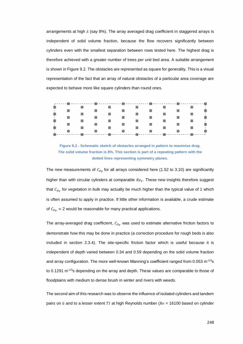
248

arrangements at high 𝜆 (say 8%). The array averaged drag coefficient in staggered arrays is

independent of solid volume fraction, because the flow recovers significantly between

cylinders even with the smallest separation between rows tested here. The highest drag is

therefore achieved with a greater number of trees per unit bed area. A suitable arrangement

is shown in Figure 9.2. The obstacles are represented as square for generality. This is a visual

representation of the fact that an array of natural obstacles of a particular area coverage are

expected to behave more like square cylinders than round ones.

Figure 9.2 - Schematic sketch of obstacles arranged in pattern to maximise drag.

The solid volume fraction is 8%. This section is part of a repeating pattern with the

dotted lines representing symmetry planes.

The new measurements of 𝐶𝐷𝑉

for all arrays considered here (1.52 to 3.10) are significantly

higher than with circular cylinders at comparable 𝑅𝑒𝑉. These new insights therefore suggest

that 𝐶𝐷𝑉 for vegetation in bulk may actually be much higher than the typical value of 1 which

is often assumed to apply in practice. If little other information is available, a crude estimate

of 𝐶𝐷𝑉≈ 2 would be reasonable for many practical applications.

The array-averaged drag coefficient, 𝐶𝐷𝑉 was used to estimate alternative friction factors to

demonstrate how this may be done in practice (a correction procedure for rough beds is also

included in section 2.3.4). The site-specific friction factor which is useful because it is

independent of depth varied between 0.34 and 0.59 depending on the solid volume fraction

and array configuration. The more well-known Manning’s coefficient ranged from 0.053 m-1/3s

to 0.1291 m-1/3s depending on the array and depth. These values are comparable to those of

floodplains with medium to dense brush in winter and rivers with weeds.

The second aim of this research was to observe the influence of isolated cylinders and tandem

pairs on �̅� and to a lesser extent 𝑇𝐼 at high Reynolds number (𝑅𝑒 = 16100 based on cylinder

249

width). This was achieved via laboratory measurements. Large fluid domains were considered

so that the wake almost fully recovered with �̅� downstream reaching values above 0.9 𝑈. This

provides test cases for numerical simulations which capture a wide range of flow behaviour.

This is useful because modelling wake velocities is important for correctly reproducing

shielding with multiple cylinders/stems. Velocity measurements with tandem pairs also provide

further physical insight into shielding. At small separation (2.5D) all velocity measurements

between the cylinders are negative and the drag is negligible. As 𝑠𝑥 increases the velocity in

the wake of the upstream cylinder has a chance to recover to some extent. By 10D the peak

velocity between cylinders reaches 0.70 𝑈. Assuming a typical isolated cylinder 𝐶𝐷 of 2.11

applies for the downstream cylinder gives an error of -47.6% in drag force predictions. If

however, the peak velocity is used in place of 𝑈 this error decreases in magnitude to 27.7%.

Although this estimate is crude, such a simple scaling is useful for estimating the forces on

sparsely arranged vegetation or other obstacles as velocities are easier to obtain in the field

than drag force measurements.

The third and final aim of this research was to evaluate the validity of the 2D realizable 𝑘-휀

turbulence model in predicting the flow around square cylinders. This was achieved by

conducting numerical simulations of the flow around isolated cylinders and tandem pairs, and

comparing the results to those of laboratory experiments. The numerical model was

successful in predicting 𝐶𝐷 of an isolated cylinder with a value of 2.19 at 𝑅𝑒 = 21400 and 𝑇𝐼 =

2%. In this regard the model performs as well as Large Eddy Simulations (LES) by other

authors with a significant increase in computational efficiency. This suggests that the model

can be applied to predict the drag on isolated bluff obstacles with similar shapes as a low-cost

alternative to LES. However, the simulation results do not capture all key aspects of flow

behaviour. In particular, the model significantly overestimates velocities in the near wake.

Further numerical simulations were then conducted to evaluate the model’s capacity to

reproduce shielding with tandem cylinders. These simulations represent another original

contribution as to the author’s knowledge the realizable 𝑘-휀 model has not been applied to

square cylinder pairs elsewhere. The model was far less successful in predicting 𝐶𝐷 of a

downstream cylinder in tandem than of a cylinder in isolation. In particular, the predicted 𝐶𝐷 is

250

less than the experimental values. At 2.5D separation, the experimentally determined value is

negligible at 0.04 but the predicted value is strongly negative at -0.60. At 10D separation, the

predicted 𝐶𝐷 of 0.76 is 46.9% lower than the experimentally determined value. This is linked

to the model’s tendency to overestimate mean velocities in the near wakes of an obstacle and

underestimate velocities further downstream. These new results suggest that the model

cannot correctly reproduce shielding effects. As such, an alternative model would need to be

considered to estimate the drag in arrays which more realistically represent vegetation.

9.2 Recommendations for Further Work

This research has highlighted a number of different areas where further work is required to

improve predictions of the drag on emergent vegetation and other obstacles in turbulent free-

surface flows. In particular, consideration should be given to:

flexibility

Reynolds number dependence

random arrays

alternative cylinder geometries

angle of attack dependence

sediment transport

number of rows dependence

numerical modelling

9.2.1 Flexibility

This research has idealised emergent vegetation as rigid which is appropriate at Cauchy

numbers less than one. This has been shown to be typical of common vegetation in wetlands

such as reeds. However, some vegetation cannot be approximated as rigid. For example,

flexible cylinders are a more appropriate model for the sedge Schoenoplectus

tabernaemontani (Chapman et al. 2015). More research is needed to better quantify the drag

on flexible vegetation. This could be achieved by idealising stems as square cylinders of

varying degrees of flexibility and determining the isolated cylinder and array-averaged drag

coefficients as functions of Cauchy number.

251

9.2.2 Reynolds Number Dependence

Laboratory results from the present study demonstrate that the assumption of a constant 𝐶𝐷𝑉

for each array provides reasonable estimates of the average drag. However, a relatively

narrow range of flow conditions were considered. In particular, the Reynolds number based

on the array-averaged velocity and cylinder width only varied between 5000 and 14200. An

alternative experiment could therefore consider the potential influence of Reynolds number on

the drag on idealised vegetation by varying both the velocity and the cylinder width.

In section 7.2 an alternative equation (Eq. (3.3)) describing the drag in cylinder arrays was

investigated:

𝐹𝐷

𝜇 𝐻 𝑈𝑉= 𝛼0 + 𝛼1𝑅𝑒

where the term on the left hand side is known as the dimensionless drag parameter and the

coefficients 𝛼0 and 𝛼1 are functions of the array configuration and solid volume fraction.

However, it was noted that more data would be required to accurately determine the

coefficients 𝛼0 and 𝛼1. This could be achieved by conducting a similar test at a greater number

of slopes. Drag force predictions based on Eq. (3.3) could then be compared to those based

on a constant drag coefficient to determine which offers the best predictions of drag force and

over what range of conditions is it necessary to consider Reynolds number effects. With the

data available this is unclear.

9.2.3 Random Arrays

In the present study the array-averaged drag coefficient was found to be different for two

random arrays at the same solid volume fraction which one would not expect for a sufficiently

long array. The cylinders were placed sequentially at a randomly assigned location within the

flow. The discrepancy in drag coefficients may therefore be a result of the arrays being too

short or it may be because the boundary locations prevented the distribution from being

sufficiently random with this method of assigning their position. This finding could therefore be

taken forward by others to determine if the drag coefficient is equal for two different long,

random arrays. If these were found to be consistent, this would give improved predictions of

the drag in rivers and wetlands as random arrays form an approximation for natural vegetation.

252

9.2.4 Alternative Cylinder Geometries

This study has idealised stems or trunks as square in cross-section thus forcing flow

separation. However, rectangular sections with alternative aspect ratios or cylinders with more

complex polygonal cross-sections could also form an approximation to some forms of

vegetation. An alternative experiment could therefore determine the individual and array-

averaged drag coefficient of cylinders with alternative geometry. This would better categorise

the influence of stem shape on the drag on vegetation.

9.2.5 Angle of Attack Dependence

The present study has focused on cylinders at zero angle of attack, 𝜗. However, Yen and

Yang (2011) demonstrated that 𝜗 can have a significant influence on the drag coefficient of

an isolated square cylinder. Data suggest that the minimum 𝐶𝐷 occurs at the critical angle of

12° and that the maximum 𝐶𝐷 occurs at 45°, although the latter is comparable to that at 0°. An

alternative experiment could therefore consider the influence of 𝜗 on cylinders in pairs or

arrays. One such experiment could consider arrays where 𝜗 is the same for each cylinder and

is non-zero. The array-averaged drag coefficient could then be compared between arrays with

different angles of attack. 45° would be of particular interest as James et al. (2008) showed

that the drag coefficient of a square cylinder at this orientation is closer to that of isolated reed

stems than the same cylinder at 𝜗 = 0°.

9.2.6 Sediment Transport

The flume used in the present study has a smooth base which is different to natural channels

such as rivers where rough sediment-covered beds are commonplace. At high solid volume

fractions the drag on even a rough bed provides a negligible contribution to the total drag

caused by the bed and the vegetation (Cheng and Nguyen 2011). However, the contribution

of a sediment-covered bed could be investigated with a model comprising of square cylinder

arrays at low solid volume fractions in a laboratory flume. This would improve our

understanding of the flow through natural channels containing sparsely distributed vegetation.

This experiment could also be extended to consider the influence of inflow conditions and

array properties on the transport of particulate materials.

253

9.2.7 Number of Rows Dependence

In section 7.1 the average 𝐶𝐷 across the front row of cylinders within a regular array of 11 rows

was found to be 54.0% higher than the isolated cylinder value. This large increase in drag is

attributed to the high fractional coverage of the cross-sectional area. One would also expect

that the presence of the rows behind would tend to raise the pressure downstream of the front

row, acting to reduce drag, but the blockage effect seems to dominate. If this explanation is

correct, the mean drag on the front row would decrease with an increase in the number of

rows. An alternative experiment could therefore determine 𝐶𝐷 as a function of position in

regular arrays with different numbers of rows. This experiment could also investigate whether

or not a larger region with a constant drag coefficient emerges as the number of rows

increases. This was observed in this research for the four rows downstream of the front row.

The drag coefficient in the constant region could also be compared with different numbers of

rows. If these were in agreement, this would suggest that this value of 𝐶𝐷 is representative of

the average drag coefficient arrays with a much larger number of cylinders. This would be

significant as measurements of the drag on one obstacle in the correct region could be taken

as representative of the entire array provided it is sufficiently long.

9.2.8 Numerical Modelling

In the present study the 2D realizable k-epsilon turbulence model was unsuccessful in

predicting the mean drag coefficients of downstream cylinders in tandem pairs. As such,

alternative numerical models would need to be considered to estimate the drag in arrays

representing vegetation. Based on this new result the author recommends expanding the

model to three-dimensions, possibly including free-surface effects, when attempting to

simulate the flow around two or more bluff obstacles with sharp edges. In addition, alternative

turbulence closures should be considered. A sensible approach would be to use several

different models to simulate the flow around tandem cylinders. The laboratory results from the

present study can be used to validate such models and the most successful could be applied

to larger arrays. Obtaining these data and providing physical insight into the variation of 𝐶𝐷

with cylinder positioning is an important first step in this process. In this regard the present

study has taken important first steps in establishing a low-cost method of simulating the flow

through rigid, emergent vegetation and other bluff obstacles in turbulent flows.

254

References

ADHIKARI, P., HONG, Y., DOUGLAS, K. R., KIRSCHBAUM, D. B., GOURLEY, J., ADLER,

R. & BRAKENRIDGE, G. R. 2010. A digitized global flood inventory (1998–2008): Compilation

and preliminary results. Natural Hazards, 55(2), 405-422.

ALBERTSON, M. L., BARTON, J. R. & SIMONS, D. B. 1960. Fluid Mechanics for Engineers,

Prentice Hall, Englewood cliffs, NJ.

BALL, D. J., STANSBY, P. K. & ALLISTON, N. 1996. Modelling shallow water flow around pile

groups. Proceedings of the Institution of Civil Engineers-Water Maritime and Energy, 118(4),

226-236.

BENNET, S. J. & SIMON, A. (Editors). 2004. Riparian Vegetation and Fluvial Geomorphology,

American Geophysical Union, Washington, DC.

BRITISH STANDARDS INSTITUTION 2005. BS EN 1991-1-4:2005. Eurocode 1: Actions on

structures – Part 1-4: General actions – Wind actions, British Standards Institution, London,

UK.

CD-ADAPCO. 2013. User Guide STAR-CCM+ Version 8.04.

CHAPMAN J. A, WILSON, B. N. & GULLIVER, J. S. 2015. Drag force parameters of rigid and

flexible vegetal elements. Water Resources Research, 51(5), 3292-3302.

CHENG, N.-S. & NGUYEN, H. T. 2011. Hydraulic Radius for Evaluating Resistance Induced

by Simulated Emergent Vegetation in Open-Channel Flows. Journal of Hydraulic Engineering,

137(9), 995-1004.

CHIN, C. S. 2012. Computer-Aided Control Systems Design: Practical Applications Using

MATLAB and Simulink, CRC Press, Boca Raton, FL.

CHURCH, M., BIRON, P. M. & ROY A. G. 2012. Gravel-bed Rivers: Processes, Tools,

Environments, Wiley-Blackwell, West Sussex, UK.

DE LANGRE, E. 2008. The effects of wind on plants: A review. Annual Review of Fluid

Mechanics, 40, 141-168.

255

ENCYCLOPAEDIA BRITANNICA. 2008. Rush. Encyclopaedia Britannica Online.

Encyclopaedia Britannica Inc. Available at: http://www.britannica.com/plant/rush-plant

[Accessed 13/06/2016].

ENCYCLOPAEDIA BRITANNICA. 2015. Rice. Encyclopaedia Britannica Online.

Encyclopaedia Britannica Inc. Available at: http://www.britannica.com/plant/rice [Accessed

13/06/2016].

ERGUN, S. 1952. Fluid flow through packed columns. Chemical Engineering Progress, 48(2),

89-94.

FARHADI, M. & RAHNAMA, M. 2005. Three-dimensional study of separated flow over a

square cylinder by large eddy simulation. Proceedings of the Institution of Mechanical

Engineers Part G: Journal of Aerospace Engineering, 219(3), 225-234.

GAO, Y. & CHOW, W. K. 2005. Numerical studies on air flow around a cube. Journal of Wind

Engineering and Industrial Aerodynamics, 93(3), 115-135.

HAMILL, L. 2001. Understanding Hydraulics, 2nd edition, Palgrave, Basingstoke, UK.

HEYWOOD, V. H. & CHANT, S. R. 1982. Popular Encylopedia of Plants, Cambridge

University Press, New York.

HINZE, J. O. 1975. Turbulence, 2nd edition, McGraw-Hill, New York.

HUTHOFF, F., AUGUSTIJN, D. C. M. & HULSCHER, S. J. M. H. 2007. Analytical solution of

the depth-averaged flow velocity in case of submerged rigid cylindrical vegetation. Water

Resources Research, 43(6), W06413.

ISHIKAWA, Y., MIZUHARA, K. & ASHIDA, S. 2000. Effect of density of trees on drag exerted

on trees in river channels. Journal of Forest Research, 5(4), 271-279.

JAMES, C. S., BIRKHEAD, A. L., JORDANOVA, A. A. & O’SULLIVAN, J. 2004. Flow

resistance of emergent vegetation. Journal of Hydraulic Research, 42(4), 390-398.

JAMES, C. S., GOLDBECK, U. K., PATINI, A. & JORDANOVA, A. A. 2008. Influence of foliage

on flow resistance of emergent vegetation, Journal of Hydraulic Research, 46(4), 536-542.

http://www.britannica.com/plant/rush-plant

http://www.britannica.com/plant/rice

256

Figure 3.18 has been reprinted from Journal of Hydraulic Research, Vol 46 issue 4, Cristopher

S. James, Uwe K. Goldbeck, Anthony Patini and Angelina A. Jordanova, Influence of foliage

on flow resistance of emergent vegetation, pages 536-542, Copyright 2008 published by

Taylor & Francis. Taylor & Francis is pleased to offer reuses of its content for a thesis or

dissertation free of charge contingent on resubmission of permission request if work is

published.

KENNISH, M. J. (Editor). 2000. Estuary Restoration and Maintenance: The National Estuary

Program, CRC Press, Boca Raton, Florida.

KOCH, D. L. & LADD, A. J. C. 1997. Moderate Reynolds number flows through periodic and

random arrays of aligned cylinders. Journal of Fluid Mechanics, 349, 31-66.

LEE, B. E. 1975. The effect of turbulence on the surface pressure field of a square prism.

Journal of Fluid Mechanics, 69(2), 263-282.

LI, R. M. & SHEN, H. W. 1973. Effects of tall vegetation on flow and sediment. Journal of the

Hydraulics Division of the American Society of Civil Engineers, 99(HY5), 793-814.

LIU, X., LEVITAN, M. & NIKITOPOULOS, D. 2008. Wind tunnel tests for mean drag and lift

coefficients on multiple circular cylinders arranged in-line. Journal of Wind Engineering and

Industrial Aerodynamics, 96(6), 831-839.

LYN, D. A., EINAV, S., RODI, W. & PARK, J. H. 1995. A laser-Doppler velocimetry study of

ensemble-averaged characteristics of the turbulent near wake of a square cylinder. Journal of

Fluid Mechanics, 304, 285-319.

MASSEY, B. S. & WARD-SMITH, J. 2006. Mechanics of Fluids, 8th edition, Taylor & Francis,

Abingdon, UK.

MATTHEWS T., MURPHY, C., WILBY R. L. & HARRIGAN, S. 2014. Stormiest winter on

record for Ireland and UK. Nature Climate Change, 4 (9), 738-740.

MEFTAH, M. B. & MOSSA, M. 2013. Prediction of channel flow characteristics through square

arrays of emergent cylinders. Physics of Fluids, 25(4), 045102.

257

MURAKAMI, S. & MOCHIDA, A. 1995. On turbulent vortex shedding flow past 2d square

cylinder predicted by CFD. Journal of Wind Engineering and Industrial Aerodynamics, 54, 191-

211.

NAUDASCHER, E., WESKE, J. R. & FEY, B. 1981. Exploratory study on damping of galloping

vibrations. Journal of Wind Engineering and Industrial Aerodynamics, 8, 211-222.

NEPF, H. M. 1999. Drag, turbulence, and diffusion in flow through emergent vegetation. Water

Resources Research, 35(2), 479-489.

NEPF, H. 2012. Hydrodynamics of Vegetated Channels. Journal of Hydraulic Research, 50(3),

262-279.

NISHINO, T., ROBERTS G. T. & ZHANG, X. 2008. Unsteady RANS and detached-eddy

simulations of flow around a circular cylinder in ground effect. Journal of Fluids and Structures,

24, 18-33.

NORBERG, C. 1993. Flow around rectangular cylinders: pressure forces and wake

frequencies. Journal of Wind Engineering and Industrial Aerodynamics, 49, 187-196.

NORTEK AS. 2004. Vectrino velocimeter user guide October 2004 Rev. c.

O’HARE, M. T. 2015. Aquatic vegetation – a primer for hydrodynamic specialists, Journal of

Hydraulic Research, 53(6), 687-698.

Figure 3.16 has been reprinted from Journal of Hydraulic Research, Vol 53 issue 6, Matthew

T. O’Hare, Aquatic vegetation – a primer for hydrodynamic specialists, pages 687-698,

Copyright 2015 published by Taylor & Francis. Taylor & Francis is pleased to offer reuses of

its content for a thesis or dissertation free of charge contingent on resubmission of permission

request if work is published.

PRIME, T., BROWN, J. M. & PLATER, A. J. 2016. Flood inundation uncertainty: The case of

a 0.5% annual probability flood event. Environmental Science & Policy, 59, 1-9.

258

RAHMAN, M., KARIM, M. & ALIM, M. 2007. Numerical investigation of unsteady flow past a

circular cylinder using 2-D finite volume method. Journal of Naval Architecture and Marine

Engineering, 4, 27-42.

ROMINGER, J. T. & NEPF, H. M. 2011. Flow adjustment and interior flow associated with a

rectangular porous obstruction. Journal of Fluid Mechanics, 680, 636-659.

ROSHKO, A. 1961. Experiments on the flow past a circular cylinder at very high Reynolds

numbers. Journal of Fluid Mechanics, 10(3), 345-356.

SCHALLER, N., KAY, A. L., LAMB, R., MASSEY, N. R., VAN OLDENBORGH, G. J., OTTO,

F. E. L., SPARROW, S. N., VAUTARD, R., YIOU, P., ASHPOLE, I., BOWERY, A., CROOKS,

S. M., HAUSTEIN, K., HUNTINGFORD, C., INGRAM, W. J., JONES, R. G., LEGG, T.,

MILLER, J., SKEGGS, J., WALLOM, D., WEISHEIMER, A., WILSON, S., STOTT, P. A. &

ALLEN, M. R. 2016. Human influence on climate in the 2014 southern England winter floods

and their impacts. Nature Climate Change, 6, 627-634.

SCHREUDER, H. T., GREGOIRE, T. G. & WOOD, G. B. 1993. Sampling Methods for

Multiresource Forest Inventory, John Wiley & Sons, New York.

SHIH, T.-H., LIOU, W. W., SHABBIR, A., YANG, Z. & ZHU, J. 1995. A new k-ϵ eddy viscosity

model for high reynolds number turbulent flows. Computers & Fluids, 24(3), 227-238.

STOESSER, T., KIM, S. J. & DIPLAS, P. 2010. Turbulent Flow through Idealized Emergent

Vegetation. Journal of Hydraulic Engineering (ASCE), 136(12), 1003-1017.

STONE, M. C., CHEN L., MCKAY S. K., GOREHAM J., ACHARYA K., FISCHENICH C. &

STONE A. B. 2013. Bending of submerged woody riparian vegetation as a function of

hydraulic flow conditions. River Research and Applications, 29, 195-205.

TANINO, Y. & NEPF, H. M. 2008. Laboratory investigation of mean drag in a random array of

rigid, emergent cylinders. Journal of Hydraulic Engineering (ASCE), 134, 34-41.

259

TAYLOR, I. & VEZZA, M. 1999. Prediction of unsteady flow around square and rectangular

section cylinders using a discrete vortex method. Journal of Wind Engineering and Industrial

Aerodynamics, 82, 247-269.

TEMMERMAN, S., MEIRE, P., BOUMA, T. J., HERMAN, P. M. J., YSEBAERT, T. & DE

VRIEND, H. J. 2013. Ecosystem-based coastal defence in the face of global change. Nature,

504, 79-83.

TIAN, X., ONG, M. C., YANG, J. & MYRHAUG, D. 2013. Unsteady RANS simulations of flow

around rectangular cylinders with different aspect ratios. Ocean Engineering, 58, 208-216.

TINER, R. W., LANG, M. W. & KLEMAS, V. V. (Editors). 2015. Remote Sensing of Wetlands,

CRC Press, Boca Raton, Florida.

TYMIŃSKI, T. & KALUŻA, Z. 2011. Investigation of mechanical properties and flow resistance

of submerged flexible riverbank vegetation. Polish Journal of Environmental Studies, 21, 201-

207.

VALLAM S., KANTHARAJ, M & LAKSHMANAN, N. 2011. Resistance of Flexible Emergent

Vegetation and Their Effects on the Forces and Runup due to Waves. The Tsunami Threat –

Research and Technology. MÃ¶rner, N.-A. (Editor), InTech.

VANONI, V. A. & BROOKS, N. H. 1957. Laboratory studies of the roughness and suspended

load of alluvial streams. Sedimentation Laboratory, California Institute of Technology,

Pasadena, California.

WADEY, M. P., BROWN, J. M., HAIGH, I. D., DOLPHIN, T. & WISSE P. 2015. Assessment

and comparison of extreme sea levels and waves during the 2013/14 storm season in two UK

coastal regions. Natural Hazards and Earth System Science, 15, 2209–2225.

WHITE, F. M. 1991. Viscous fluid flow, 2nd edition, McGraw-Hill, New York.

WOLFSHTEIN, M. 1969. The velocity and temperature distribution in one-dimensional flow

with turbulence augmentation and pressure gradient. International Journal of Heat and Mass

Transfer, 12(3), 301-318.

260

WUNDER S., LEHMANN B. & NESTMANN, F. 2011. Determination of the drag coefficients

of emergent and just submerged willows. International Journal of River Basin Management,

9(3-4), 231-236.

YEN, S. C. & LIU, J. H. 2011. Wake flow behind two side-by-side square cylinders.

International Journal of Heat and Fluid Flow, 32, 41-51.

YEN, S. C., SAN, K. C. & CHUANG, T. H. 2008. Interactions of tandem square cylinders at

low Reynolds numbers. Experimental Thermal and Fluid Science, 32(4), 927-938.

YEN, S. C. & YANG, C. W. 2011. Flow patterns and vortex shedding behavior behind a square

cylinder. Journal of Wind Engineering and Industrial Aerodynamics, 99(8), 868-878.

Figure 3.8 has been reprinted from Journal of Wind Engineering and Industrial Aerodynamics,

Vol 99 issue 8, Shun C. Yen and Chen W. Yang, Flow patterns and vortex shedding behavior

behind a square cylinder, pages 868-878, Copyright 2011 with permission from Elsevier.

ZDRAVKOVICH, M. M. & PRIDDEN, D. L. 1977. Interference between 2 circular cylinders;

series of unexpected discontinuities. Journal of Industrial Aerodynamics, 2(3), 255-270.

ZHANG, H., WANG, Z., DAI, L., & XU, W. 2015. Influence of Vegetation on Turbulence

Characteristics and Reynolds Shear Stress in Partly Vegetated Channel. Journal of Fluids

Engineering, 137(6), 061201-061201-8.

Figure 3.17 has been reprinted from Journal of Fluids Engineering, Vol 137 issue 6, Huayong

Zhang, Zhongyu Wang, Liming Dai and Weigang Xu, Influence of Vegetation on Turbulence

Characteristics and Reynolds Shear Stress in Partly Vegetated Channel, pages 061201-

061201-8, Copyright 2015 with permission from ASME.

Documents

An Experimental Investigation of the Drag on Idealised