An experimental investigation of the geometric ... · The geometric characteristics of flapping-wing propulsion are studied experimentally through ... DARPA’s specifications for

Calhoun: The NPS Institutional Archive

Theses and Dissertations Thesis Collection

2003-06

An experimental investigation of the geometric

characteristics of flapping-wing propulsion for a

micro-air vehicle

Papadopoulos, Jason N.

Monterey, California. Naval Postgraduate School

http://hdl.handle.net/10945/936

NAVAL POSTGRADUATE SCHOOL Monterey, California

THESIS

Approved for public release; distribution is unlimited.

AN EXPERIMENTAL INVESTIGATION OF THE GEOMETRIC CHARACTERISTICS OF FLAPPING-WING PROPULSION

FOR A MICRO AIR VEHICLE by

Jason Papadopoulos

June 2003

Thesis Advisor: Kevin D. Jones Co-Advisor: Max F. Platzer

THIS PAGE INTENTIONALLY LEFT BLANK

i

REPORT DOCUMENTATION PAGE Form Approved OMB No. 0704-0188

Public reporting burden for this collection of information is estimated to average 1 hour per response, including the time for reviewing instruction, searching existing data sources, gathering and maintaining the data needed, and completing and reviewing the collection of information. Send comments regarding this burden estimate or any other aspect of this collection of information, including suggestions for reducing this burden, to Washington headquarters Services, Directorate for Information Operations and Reports, 1215 Jefferson Davis Highway, Suite 1204, Arlington, VA 22202-4302, and to the Office of Management and Budget, Paperwork Reduction Project (0704-0188) Washington DC 20503. 1. AGENCY USE ONLY (Leave blank)

2. REPORT DATE June 2003

3. REPORT TYPE AND DATES COVERED Master’s Thesis

4. TITLE AND SUBTITLE: An Experimental Investigation of the Geometric Characteristics of Flapping-Wing Propulsion for a Micro Air Vehicle

6. AUTHOR(S)

5. FUNDING NUMBERS

7. PERFORMING ORGANIZATION NAME(S) AND ADDRESS(ES) Naval Postgraduate School Monterey, CA 93943-5000

8. PERFORMING ORGANIZATION REPORT NUMBER

9. SPONSORING /MONITORING AGENCY NAME(S) AND ADDRESS(ES) N/A

10. SPONSORING/MONITORING AGENCY REPORT NUMBER

11. SUPPLEMENTARY NOTES The views expressed in this thesis are those of the author and do not reflect the official policy or position of the Department of Defense or the U.S. Government.

12a. DISTRIBUTION / AVAILABILITY STATEMENT Approved for public release; distribution is unlimited.

12b. DISTRIBUTION CODE

13. ABSTRACT (maximum 200 words) The geometric characteristics of flapping-wing propulsion are studied experimentally through the use of a force balance and a Micro Air Vehicle (MAV) system. The system used is built to duplicate the propulsion system currently on the flying model of the Naval Postgraduate School (NPS) MAV model. Experiments are carried out in a low speed wind tunnel to determine the effects of mean separation and plunge amplitude on the flapping wing propulsion system. Additionally, the effects of flapping-wing shape, flapping frequency, and MAV angle of attack (AOA) are also investigated. Some flow visualization is also performed. The intent is to optimize the system so that payload and controllability improvements can be made to the NPS MAV.

15. NUMBER OF PAGES

89

14. SUBJECT TERMS Micro Air Vehicle, Flapping-Wing Propulsion, Force Balance, Flow Visualization

16. PRICE CODE

17. SECURITY CLASSIFICATION OF REPORT

Unclassified

18. SECURITY CLASSIFICATION OF THIS PAGE

Unclassified

19. SECURITY CLASSIFICATION OF ABSTRACT

Unclassified

20. LIMITATION OF ABSTRACT

UL

NSN 7540-01-280-5500 Standard Form 298 (Rev. 2-89) Prescribed by ANSI Std. 239-18

ii


iii

Approved for public release; distribution is unlimited.

AN EXPERIMENTAL INVESTIGATION OF THE GEOMETRIC CHARACTERISITCS OF FLAPPING-WING PROPULSION FOR A MICRO-AIR

VEHICLE

Jason N. Papadopoulos Ensign, United States Navy Reserve

B.S. Mechanical Engineering, University of Texas, 2002

Submitted in partial fulfillment of the requirements for the degree of

MASTER OF SCIENCE IN AERONAUTICAL ENGINEERING

from the

NAVAL POSTGRADUATE SCHOOL June 2003

Author: Jason Papadopoulos Approved by: Dr. Kevin Jones

Thesis Advisor

Dr. Max Platzer Co-Advisor Dr. Max Platzer Chairman, Department of Aeronautics and Astronautics

iv


v

ABSTRACT

The geometric characteristics of flapping-wing

propulsion are studied experimentally through the use of a

force balance and a Micro Air Vehicle (MAV) system. The

system used is built to duplicate the propulsion system

currently on the flying model of the Naval Postgraduate

School (NPS) MAV model. Experiments are carried out in a

low speed wind tunnel to determine the effects of mean

separation and plunge amplitude on the flapping wing

propulsion system. Additionally, the effects of flapping-

wing shape, flapping frequency, and MAV angle of attack

(AOA) are also investigated. Some flow visualization is

also performed. The intent is to optimize the system so

that payload and controllability improvements can be made

to the NPS MAV.

vi


vii

TABLE OF CONTENTS

I. INTRODUCTION ............................................1

A. OVERVIEW ...........................................1 B. BACKGROUND .........................................1 C. FLAPPING-WING PROPULSION ...........................3

II. EXPERIMENTAL SETUP ......................................7 A. PROPUSLION SYSTEM ..................................7 B. FORCE BALANCE .....................................10 C. WIND TUNNEL .......................................11 D. DATA ACQUISITION SYSTEM ...........................13

III. EXPERIMENTAL ANALYSIS ................................15 A. CALIBRATION .......................................15

1. Lift .........................................15 2. Thrust .......................................18 3. Motor Voltage and Motor Current ..............21 4. Motor Shaft Power ............................22

a. MAV Motor Shaft Power ...................25 B. EXPERIMENTAL METHOD ...............................26

1. Test Procedures ..............................26 2. Test Geometries ..............................28

a. Standard Model ..........................29 b. Standard Model 2 ........................31 c. Standard Model 3 ........................32

C. DATA REDUCTION ....................................33 1. Cycles .......................................33 2. Figure of Merit ..............................33 3. Error Analysis ...............................33

a. Error Calculation .......................35 IV. EXPERIMENTAL RESULTS ...................................37

A. MAV MOTOR .........................................37 B. STANDARD MODEL ....................................37 C. STANDARD MODEL WITH MAIN WINGS ....................40 D. STANDARD MODEL 2 ..................................41 E. STANDARD MODEL 3 ..................................44 F. FLOW VISUALIZATION ................................47

V. CONCLUSIONS ............................................51 VI. RECOMMENDATIONS ........................................53 APPENDIX A. MATLAB CODE FOR CALCULATING EXPERIMENTAL

OFFSET VALUES ..........................................55

viii

APPENDIX B. MATLAB CODE FOR CALCULATING EXPERIMENTAL THRUST AND LIFT VALUES .................................57

APPENDIX C. EXPERIMENTAL DATA FOR STANDARD MODEL WITH LIFTING WINGS ..........................................61

APPENDIX D. EXPERIMENTAL DATA FOR STANDARD MODEL 2 .........65 APPENDIX E. EXPERIMENTAL DATA FOR STANDARD MODEL 3 .........69 LIST OF REFERENCES ..........................................73 INITIAL DISTRIBUTION LIST ...................................75

ix

LIST OF FIGURES

Figure 1. Black Widow MAV...................................2 Figure 2. AeroVironment Microbat............................3 Figure 3. Knoller-Betz Effect...............................4 Figure 4. Wave Propeller Setup..............................5 Figure 5. Opposed-Plunge Setup..............................5 Figure 6. NPS Prototype MAV.................................6 Figure 7. Motor Circuit Schematic...........................8 Figure 8. Test Model Propulsion System.....................10 Figure 9. Schematic of NPS Low-Speed Wind Tunnel...........12 Figure 10. Schematic of Experimental Setup..................14 Figure 11. Lift Calibration Curve...........................17 Figure 12. Lift Channel Interference on Thrust Channel......18 Figure 13. Thrust Calibration Curve.........................20 Figure 14. Thrust Channel Interference in Lift Channel......21 Figure 15. Mechanical Power From Test Motor.................24 Figure 16. Mechanical Power From MAV Motor..................25 Figure 17. MAV Motor Efficiency.............................26 Figure 18. Standard Model Schematic.........................29 Figure 19. Flapping Wings Used in Experiments...............30 Figure 20. Standard Model with Main wings...................31 Figure 21. Standard Model 2 Schematic.......................32 Figure 22. Standard Model 3 Schematic.......................32 Figure 23. Thrust vs. Frequency, 0deg AOA, V=0 m/s, SM......38 Figure 24. Thrust vs. Frequency, 10deg AOA, V=0 m/s, SM.....38 Figure 25. Thrust vs. Frequency, V=4 m/s, SM................39 Figure 26. Thrust vs. Frequency, 0deg AOA, V=3 m/s, SM......40 Figure 27. Thrust vs. Frequency, 10deg AOA, V=3 m/s, SM.....41 Figure 28. Thrust vs. Frequency, V=0 m/s, SM2...............42 Figure 29. Thrust vs. Frequency, V= 3m/s, SM2...............42 Figure 30. Lift vs. Frequency, V=3 m/s, SM2.................43 Figure 31. Thrust vs. Frequency, V=0 m/s, SM3...............44 Figure 32. Thrust vs. Frequency, V=3 m/s, SM3...............44 Figure 33. Lift vs. Frequency, V=3 m/s, SM3.................46 Figure 34. Flow Separation, V=2.5 m/s, 0 Hz, SM.............47 Figure 35. Flow Separation, V=2.5 m/s, 31 Hz, SM............48 Figure 36. Flow Seperation, V=2.5 m/s, 0 Hz, SM3............48 Figure 37. Flow Remains Attached, V=2.5 m/s, 31 Hz, SM3.....49

x


xi

ACKNOWLEDGMENTS

The author would like to express his sincerest

gratitude to Dr. Kevin Jones for his time and efforts

supervising and assisting in the completion of this

project. Additionally, he would like to thank Dr. Max

Platzer for his oversight and encouragement.

The author would also like to thank Professor Art

Schoenstadt for his aid in the creation of the MATLAB codes

used for this paper.

Finally, the author would like to thank his family for

their continuing support and encouragement throughout the

years, without whom this would not have been possible.

xii


1

I. INTRODUCTION

A. OVERVIEW

This paper examines the geometric characteristics of a

flapping-wing Micro Air Vehicle (MAV) propulsion system in

order to determine their effects on the lift and thrust

produced by the system. This study builds on work that has

been carried out over the past several years at the Naval

Postgraduate School (NPS). The ultimate goal of this paper

is to aid in the research and development of a flight

worthy, remote-controlled MAV.

All experiments were carried out in the NPS 1.5 m x

1.5 m wind tunnel. The MAV models used in the experiments

were chosen to closely imitate the construction of the MAV

model developed at NPS that has already demonstrated

capability for controlled flight. In order to obtain lift

and thrust measurements the propulsion system was sting

mounted through the floor of the wind tunnel and connected

to a force balance. Professor Kevin Jones previously

developed all of the MAV component parts as well as the

force balance. Finally, some flow visualization

experiments were carried out to help understand flow

behavior.

B. BACKGROUND

In 1997, the Defense Advanced Research Projects Agency

(DARPA) became interested in the possibility of using MAVs

in military operations; their inherent ability for

reconnaissance and surveillance missions being the primary

focus. DARPA’s specifications for the MAV were that it be,

“an affordable, fully functional, military capable, flight

2

vehicle, limited to 15 cm in length, width or height.”

[Ref. 1]. Additionally, it was required that the MAV be

able to sustain flight times of at least 20 minutes, have a

range of 10 km, and a payload capability of 20 grams.

The war in Afghanistan made the need for a flight

capable MAV even more apparent. The perilous job of

searching caves for hostile activity could have been

accelerated while at the same time reducing personnel risks

to soldiers on the ground. The capability of an advanced

warning system using MAVs to locate snipers and enemy

positions would have greatly aided soldiers in an urban

combat environment. Additionally, the CIA had also

expressed interest in employing MAVs in a variety of

different surveillance missions.

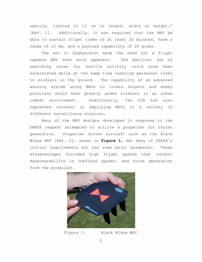
Many of the MAV designs developed in response to the

DARPA request attempted to utilize a propeller for thrust

generation. Propeller driven aircraft such as the Black

Widow MAV [Ref. 2], shown in Figure 1, met many of DARPA’s

initial requirements but had some major drawbacks. These

disadvantages included high flight speeds that inhibit

maneuverability in confined spaces, and noise generation

from the propeller.

Figure 1. Black Widow MAV

3

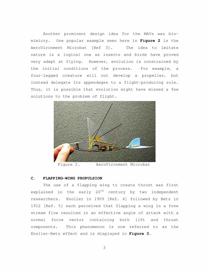
Another prominent design idea for the MAVs was bio-

mimicry. One popular example seen here in Figure 2 is the

AeroVironment Microbat [Ref 3]. The idea to imitate

nature is a logical one as insects and birds have proved

very adept at flying. However, evolution is constrained by

the initial conditions of the process. For example, a

four-legged creature will not develop a propeller, but

instead delegate its appendages to a flight-producing role.

Thus, it is possible that evolution might have missed a few

solutions to the problem of flight.

Figure 2. AeroVironment Microbat

C. FLAPPING-WING PROPULSION

The use of a flapping wing to create thrust was first

explained in the early 20th century by two independent

researchers. Knoller in 1909 [Ref. 4] followed by Betz in

1912 [Ref. 5] each perceived that flapping a wing in a free

stream flow resulted in an effective angle of attack with a

normal force vector containing both lift and thrust

components. This phenomenon is now referred to as the

Knoller-Betz effect and is displayed in Figure 3.

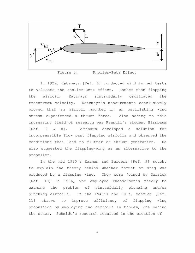
4

Figure 3. Knoller-Betz Effect

In 1922, Katzmayr [Ref. 6] conducted wind tunnel tests

to validate the Knoller-Betz effect. Rather than flapping

the airfoil, Katzmayr sinusoidally oscillated the

freestream velocity. Katzmayr’s measurements conclusively

proved that an airfoil mounted in an oscillating wind

stream experienced a thrust force. Also adding to this

increasing field of research was Prandtl’s student Birnbaum

[Ref. 7 & 8]. Birnbaum developed a solution for

incompressible flow past flapping airfoils and observed the

conditions that lead to flutter or thrust generation. He

also suggested the flapping-wing as an alternative to the

propeller.

In the mid 1930’s Karman and Burgers [Ref. 9] sought

to explain the theory behind whether thrust or drag was

produced by a flapping wing. They were joined by Garrick

[Ref. 10] in 1936, who employed Theodorsen’s theory to

examine the problem of sinusoidally plunging and/or

pitching airfoils. In the 1940’s and 50’s, Schmidt [Ref.

11] strove to improve efficiency of flapping wing

propulsion by employing two airfoils in tandem, one behind

the other. Schmidt’s research resulted in the creation of

5

the wave propeller (See Figure 4), which he claimed

achieved efficiencies as good as those of conventional

propellers.

Figure 4. Wave Propeller Setup

More recently, Jones and Platzer [Ref 12 & 13] studied

Schmidt’s wave propeller and also examined other wake

interference configurations. The most promising of these

configurations was the opposed plunge configuration shown

in Figure 5. The opposed plunge configuration attempted to

produce and take advantage of ground-effect conditions

similar to when a bird flies close to the water’s surface.

Its many benefits included being mechanically and

aerodynamically balanced, as well as producing greater

thrust than the wave propeller configuration. In the last

few years, Jones and Platzer have customized the opposed

plunge configuration to be used as the propulsion system

for a MAV they developed [Ref. 13]. The first sustained

flight took place in December of 2003, and further research

into controllability and durability issues is currently

being studied.

Figure 5. Opposed-Plunge Setup

6

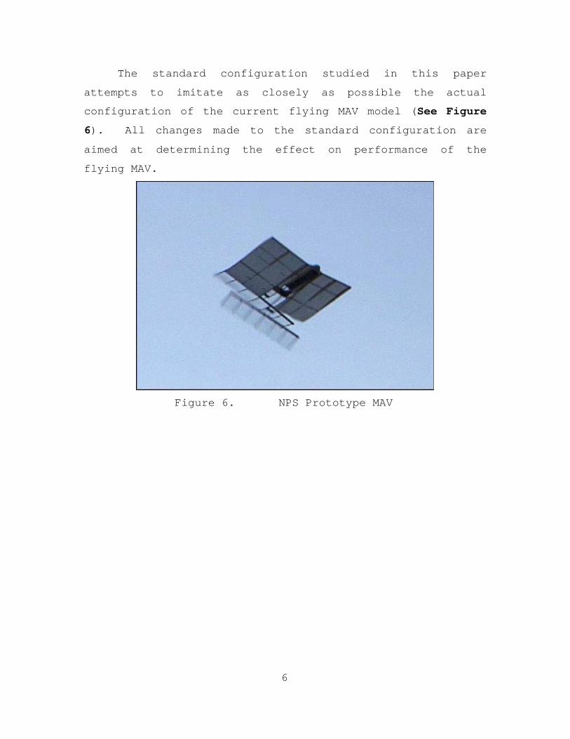
The standard configuration studied in this paper

attempts to imitate as closely as possible the actual

configuration of the current flying MAV model (See Figure

6). All changes made to the standard configuration are

aimed at determining the effect on performance of the

flying MAV.

Figure 6. NPS Prototype MAV

7

II. EXPERIMENTAL SETUP

A. PROPUSLION SYSTEM

The motor used to drive the NPS MAV is 1.2 volt pager

motor that is run at 5 volts to increase power density.

The lifespan of small motors under these conditions are not

conducive to prolonged experimental analysis because of

brush wear problems. Consequently, the propulsion system

used during experimentation incorporated a Faulhaber direct

current motor with an independent power source. It was

powered by an ELENCO MX-9300 Power Supply from which the

voltage into the motor was varied. The shaft speed of the

motor was slowed down using a 37:1 planetary gear system.

With this gear ratio, the frequency of the rotating shaft

powering the flapping wings could be made to closely mimic

those found in the actual MAV models.

A resistor with a 0.011 ohm resistance was placed in

series with the motor in order to measure the motor

current. Since the drop in voltage across the resistor was

negligible compared to the voltage drop across the motor,

the motor voltage reading was unaffected. However, an

amplifier was needed to add a fixed gain to the voltage

drop across the resistor so it could be read accurately by

the data acquisition system. The voltage drop across the

resistor was later converted to current when the data was

analyzed. Both the motor voltage and the voltage drop

representing the motor current were fed into the data

acquisition system. A circuit block was built to

facilitate the connection of leads to the motor circuit. A

diagram of the motor circuit can be seen in Figure 7.

8

Figure 7. Motor Circuit Schematic

In order to measure the propulsion shaft speeds, an

aluminum disk containing a notch was placed onto the slowed

down shaft. A light beam whose path was interrupted by the

disk could only strike a photosensitive diode when the

notch was lined up with the light beam. This diode

completed a circuit that had a fixed voltage. When the

shaft rotated, the effect was that the voltage in the

diode’s circuit had the form of a square wave. This

voltage was fed into a signal conditioner and then into the

data acquisition system. The speed of the shaft powering

the flapping wings was found by using the sample rate of

the data acquisition system to determine the time from the

9

start of one square wave to the next. The square wave was

also fed into an oscilloscope to allow for real-time

frequency readings.

A crankshaft was used to change the rotational motion

of the shaft into linear movement. Connecting rods linked

the crankshaft to a set of flapping beams that produced the

desired motion. The size of the crankshaft and connecting

rods governed the plunge amplitude and mean separation of

the wings. The flapping beams were screwed on the front

end to a composite case that contained the motor and gear

system, while the flapping wings were attached to the other

end. The leading edge of the flapping wing was cylindrical

with tapered ends and constructed from a thin dowel of

balsa wood. The rest of the wing surface was lightweight

plastic laminate. Support ribs made from carbon-fiber ran

from the leading edge to the trailing edge of these wings.

The wings were super-glued to the flapping beams via a thin

carbon fiber strip. The stiffness of this strip governs

the pitch angle oscillations found in the wing and allow

for a passive feathering mechanism [Ref. 14]. A picture of

the complete propulsion system can be seen in Figure 8.

Dr. Kevin Jones built all MAV components, and further

details on the construction of these parts can be found in

reference 13.

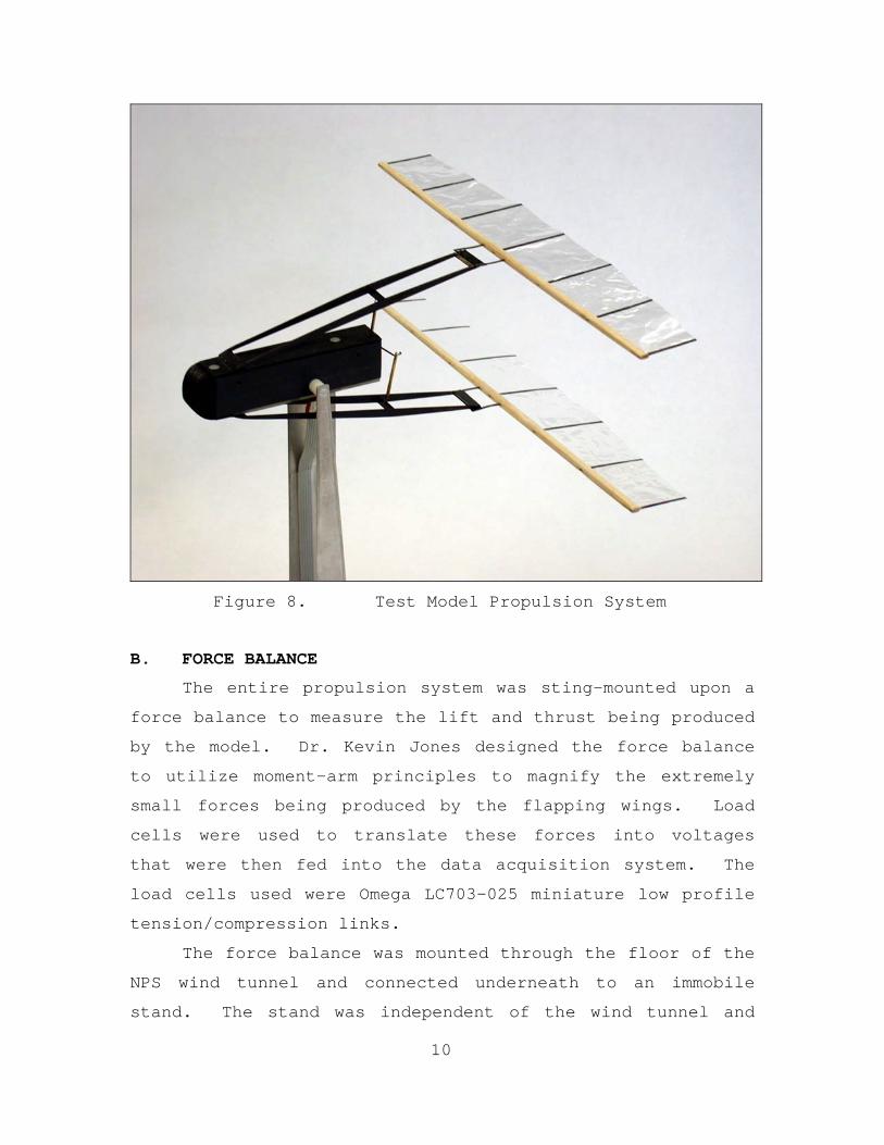
10

Figure 8. Test Model Propulsion System

B. FORCE BALANCE

The entire propulsion system was sting-mounted upon a

force balance to measure the lift and thrust being produced

by the model. Dr. Kevin Jones designed the force balance

to utilize moment-arm principles to magnify the extremely

small forces being produced by the flapping wings. Load

cells were used to translate these forces into voltages

that were then fed into the data acquisition system. The

load cells used were Omega LC703-025 miniature low profile

tension/compression links.

The force balance was mounted through the floor of the

NPS wind tunnel and connected underneath to an immobile

stand. The stand was independent of the wind tunnel and

11

prevented any vibrations of the wind tunnel walls from

corrupting the force balance readings. The distance from

the floor of the wind tunnel to the bottom of the model was

measured to be two feet. This placed the flapping wings

near the center of the wind tunnel test section, but

allowed for laser Doppler velocimetry (LDV) above the

centerline.

C. WIND TUNNEL

All experimentation was conducted in the NPS low-speed

wind tunnel illustrated in Figure 9. The wind tunnel has a

4.5m x 4.5 m square inlet that converges to a 1.5m x 1.5m

test section. Tunnel speeds vary from 0 to 9.5 m/s, and

are controlled by a variable pitch fan powered by a

constant speed electric motor. Rubber sleeves are used to

isolate the vibrations of the fan assembly from the test

section.

12

Figure 9. Schematic of NPS Low-Speed Wind Tunnel

During experimentation a pitot-static tube was used to

determine the tunnel velocity. The pitot tube was located

directly above the model, and approximately 1.5 feet below

the ceiling of the test section. A MKS Baratron type 223B

differential pressure transducer took the pressure seen by

the pitot tube, and converted it to a voltage which was

read by a Metex 3610D digital multimeter. The tunnel speed

was calculated using Bernoulli’s equation and the

conversion ratio of the pressure transducer (1 volt per

133.2 Pa).

13

D. DATA ACQUISITION SYSTEM

All of the signal lines from the propulsion system and

force balance were fed into an Omega Screw Terminal Block.

The signals wired into the block based on their channel

number location were:

Channel 1: Rotary Encoder

Channel 2: Lift from Force Balance

Channel 3: Thrust from Force Balance

Channel 5: Motor Voltage

Channel 6: Motor Current

The pressure transducer voltage was initially supposed to

be wired as Channel 4 so that real-time velocity

measurements could be taken. However, all attempts to hook

up the pressure transducer to the screw terminal block (in

Channel 4 and other locations as well) resulted in ground

loop problems and cross-talk between the channels. Without

the transducer hookup, no interference was seen between the

channels. Thus, the transducer velocity was read from the

multimeter directly, and Channel 4 was left unused.

The data acquisition card used in our experiments was

an Omega DAQP-16-OM-A Type II PCMCIA card. It had an

effective range of +/- 10 volts and used twos complement

16-bit precision to read and store the data. The card was

hooked directly to a laptop PC and was controlled using the

program DaqEZ Version 4.11. Using this program the sample

rate and duration of each measurement could be controlled,

and the data files stored directly to the laptop hard

drive. A schematic summarizing the complete setup can be

seen in Figure 10.

14

Figure 10. Schematic of Experimental Setup

15

III. EXPERIMENTAL ANALYSIS

A. CALIBRATION

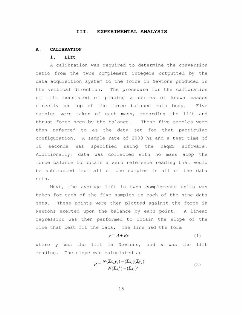
1. Lift

A calibration was required to determine the conversion

ratio from the twos complement integers outputted by the

data acquisition system to the force in Newtons produced in

the vertical direction. The procedure for the calibration

of lift consisted of placing a series of known masses

directly on top of the force balance main body. Five

samples were taken of each mass, recording the lift and

thrust force seen by the balance. These five samples were

then referred to as the data set for that particular

configuration. A sample rate of 2000 hz and a test time of

10 seconds was specified using the DaqEZ software.

Additionally, data was collected with no mass atop the

force balance to obtain a zero reference reading that would

be subtracted from all of the samples in all of the data

sets.

Next, the average lift in twos complements units was

taken for each of the five samples in each of the nine data

sets. These points were then plotted against the force in

Newtons exerted upon the balance by each point. A linear

regression was then performed to obtain the slope of the

line that best fit the data. The line had the form

BxAy += (1)

where y was the lift in Newtons, and x was the lift

reading. The slope was calculated as

22 )()())(()(

ii

iiii

xxNyxyxN

BΣ−Σ

ΣΣ−Σ= (2)

16

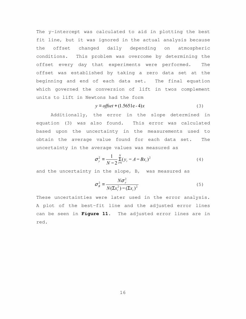
The y-intercept was calculated to aid in plotting the best

fit line, but it was ignored in the actual analysis because

the offset changed daily depending on atmospheric

conditions. This problem was overcome by determining the

offset every day that experiments were performed. The

offset was established by taking a zero data set at the

beginning and end of each data set. The final equation

which governed the conversion of lift in twos complement

units to lift in Newtons had the form

xoffsety 4)-1.5651e(+= (3)

Additionally, the error in the slope determined in

equation (3) was also found. This error was calculated

based upon the uncertainty in the measurements used to

obtain the average value found for each data set. The

uncertainty in the average values was measured as

2

1

2 )(2

1ii

N

iy BxAyN

−−Σ−

==

σ (4)

and the uncertainty in the slope, B, was measured as

22

22

)()( ii

yB xxN

NΣ−Σ

=σ

σ (5)

These uncertainties were later used in the error analysis.

A plot of the best-fit line and the adjusted error lines

can be seen in Figure 11. The adjusted error lines are in

red.

17

Figure 11. Lift Calibration Curve

Lastly, a plot was made of the average thrust force in

twos complement units versus the average lift force in twos

complements units (See Figure 12). This graph represented

the cross talk between the lift and thrust components on

the force balance. The total vertical difference between

the highest and lowest value of the thrust was divided by

two and used as the error estimate in the thrust channel as

a result of lift forces.

18

Figure 12. Lift Channel Interference on Thrust Channel

2. Thrust

The conversion of thrust from twos complement units to

Newtons was nearly identical to the lift conversion. The

main difference between the two lay in the setup. In order

to generate horizontal forces of a known magnitude a string

was attached to the sting mounted propulsion system. This

string ran over a pulley and had a mass tied to the

opposite end. Care was taken to insure that the string

remained horizontal until it reached the pulley so that

cross talk in the lift direction would be minimized. A

series of masses identical to those used in the lift

calibration were then hung on the opposite end of the

string. Both the thrust and lift data was recorded and

19

again, five samples were taken with each mass using the

same sample rate and test time as the lift calibration.

The techniques used to analyze the thrust data sets

were identical to those used in the lift calibration.

Averages were taken for each data set and plotted against

the true thrust force in Newtons. A best-fit line was

fitted to this plot using the same formulas as shown in

equations (1) and (2). The only difference was that this

time the variable y represented the thrust in Newtons, and

x represented the thrust in twos complement units. The

final equation that governed the conversion of thrust into

Newtons was given by

( )xey 57349.5offset = −+ (6)

The y-intercept was again ignored and calculated whenever

experiments were conducted. The error in the slope was

computed using equations (4) and (5), and the adjusted

lines were plotted against the best-fit line (See Figure

13). The error in the thrust calibration curve was again

taken as the maximum difference between any of these lines.

20

Figure 13. Thrust Calibration Curve

Finally, a plot of the interference of the thrust force on

the lift was created, and an estimate of the error in the

lift force due to thrust was obtained (See Figure 14).

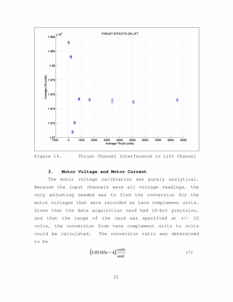
21

Figure 14. Thrust Channel Interference in Lift Channel

3. Motor Voltage and Motor Current

The motor voltage calibration was purely analytical.

Because the input channels were all voltage readings, the

only adjusting needed was to find the conversion for the

motor voltages that were recorded as twos complement units.

Given that the data acquisition card had 16-bit precision,

and that the range of the card was specified at +/- 10

volts, the conversion from twos complement units to volts

could be calculated. The conversion ratio was determined

to be

( )unitvoltse 405185.3 − (7)

22

The motor current read by the data acquisition system

was actually the amplified voltage drop across a small

resistor (See Figure 7). The gain on the amplifier was

unknown so a calibration test was needed. During

calibration a known resistance replaced the motor and a

fixed voltage was passed through the circuit. The voltage

drop across the small resistor was calculated and compared

to the voltage coming out of the amplifier. The ratio of

the two was the gain given to the signal. This process was

repeated using three different resistances to replace the

motor. The average of these three trial runs was used as

the gain on the amplifier, and the standard deviation was

used as the approximate error in the gain. The gain was

calculated to be 256. With this value for the gain, the

conversion of twos complement units to volts representative

of the current was calculated to be

( )unitvoltse 69005.1 − (8)

These voltages were then divided by the resistance of the

small resistor, 0.011 ohms, to give the actual current in

amperes running through the motor.

4. Motor Shaft Power

The mechanical power produced by the motor and gear-

drive assembly was needed to calculate meaningful

efficiencies. In order to determine this power a special

setup was needed. The wings, flapping beams, and all other

associated parts were removed from the propulsion system.

A spindle was then attached to the motor shaft and a very

thin (0.005” diameter) copper wire super-glued to the

spindle. The wire ran up and over a pulley approximately

two feet above the motor shaft and then down four feet to

the floor. A series of different masses were hung from the

23

copper wire and data sets were taken while the motor wound

up the wire and raised the mass. Each mass was wound up

using an increasing set of motor voltages.

The shaft-power was calculated as rotational shaft

speed multiplied by the shaft torque. The shaft torque was

the weight of the mass tied to the string multiplied by the

sum of the radius of the spindle and half a thread width.

The calculation of the shaft rotational speed is explained

in the experimental setup.

The data from the calculations showed that the masses

below thirty grams were indistinguishable from one another;

all seemed to require the same amount of input power from

the motor. Clearly this was incorrect, as the current

should increase with mass for a given voltage. Therefore,

the readings below thirty grams were omitted, and a cubic

interpolation was attempted based on the sparse data of the

upper three readings, and a zero set (See Figure 15). The

zero set assumed that the current was nearly zero (0.01

amperes) regardless of the range, and that the shaft power

was zero.

24

Figure 15. Mechanical Power From Test Motor

Initially the interpolation seemed reasonable,

however, later testing and analysis showed that the values

specified in Figure 15 were too low to be accurate. The

power output values from the graph were yielding figures of

merit an order of magnitude greater than that produced by

the test MAV. The problem was that by choosing an

oversized motor, the motor friction was also increased.

The torque necessary to overcome this friction was of the

same magnitude of the torque necessary to flap the wings.

Thus, the noise from the motor friction prevented accurate

torque measurements in the lower regions. Unfortunately,

this is the region in which the flapping wings operate.

Therefore, Figure 15 was determined to be inaccurate and

25

efficiency calculations were not performed using the large

motor.

a. MAV Motor Shaft Power

The same setup used to calculate the motor shaft

power of the propulsion system was also used to calculate

the shaft power of the motor used in the flying MAV.

However, with the MAV motor the problems of motor friction

were not an issue due to its smaller size and design for

lower voltages. As a result, accurate measurements were

taken and the MAV motor shaft power as well as its

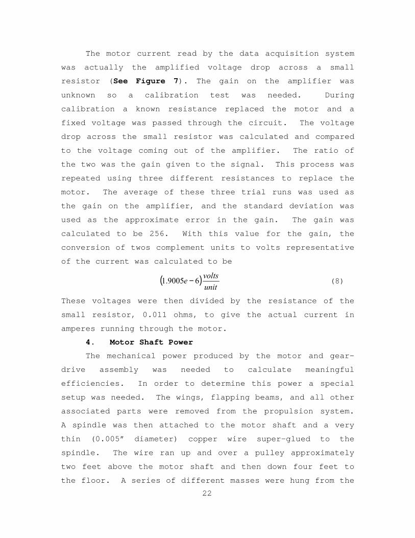
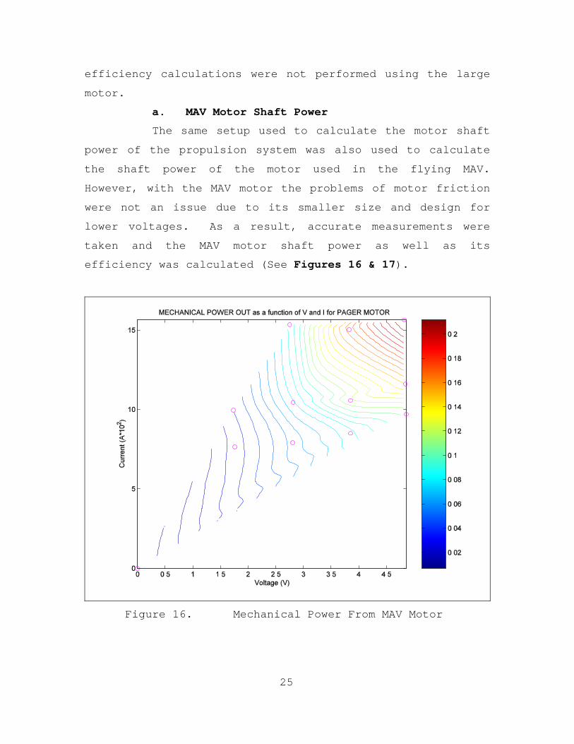
efficiency was calculated (See Figures 16 & 17).

Figure 16. Mechanical Power From MAV Motor

26

Figure 17. MAV Motor Efficiency

To date the only flying MAV model used a motor

identical to the one tested here. That MAV was measured to

draw 5 volts at approximately 0.3 amperes.

B. EXPERIMENTAL METHOD

1. Test Procedures

The same procedure was used for each geometric variant

of the MAV components that were tested. First, the MAV

components were setup on the sting connected to the force

balance. Once the components were attached, the angle of

attack (AOA) of the model was set to zero degrees. The AOA

27

was measured as the angle that the top surface of the

fuselage made with the horizontal. The angle was measured

using an angle finder.

Once the model was set to an AOA of zero degrees, the

motor voltage was set to approximately 5 volts and a data

set obtained. Each data set consisted of five samples

measured with a sample rate of 2000 HZ for 10 seconds. The

values measured in each data set were the 5 lines entering

the data acquisition system discussed previously. The

motor voltage was then increased incrementally from 5 volts

to approximately 10 or 17 volts, with one data set taken at

every voltage in between. Initially, 10 volts was set as

the limit because of the range constraints of the DAQ card

in reading the motor voltage. However, after it was

discovered that efficiency could not be calculated,

Channels 5 and 6 were disconnected and the motor was run at

the higher voltages. These higher voltages yielded

flapping frequencies similar to the flying MAV model.

Additionally, two data sets were obtained with no

motor power, before and after all the other data sets had

been taken. These two data sets were averaged and then

used as the thrust offset value for the six data sets taken

with the motor running. The total difference between the

two offset data sets was used as the drift error for all of

the motor voltage data sets they spanned.

After the last offset data set had been taken, the

velocity of the wind tunnel was increased. The AOA was

held constant and the entire process was repeated again for

a new tunnel velocity. The tunnel velocities tested ranged

from approximately 0–4 m/s. Once all of the tunnel

28

velocities had been tested for one particular AOA, the wind

tunnel was shut down, a new AOA was set, and the entire

process repeated.

The only difference between any of the samples taken

involved the thrust offset data sets when the tunnel speeds

were not zero. For these data sets the motor voltage was

not set to 0 volts as described above, but instead to 0.7

volts. At 0.7 volts the flapping wings moved very slowly

and created no effective thrust. This was done to account

for the different profile drag characteristics of the

flapping wings when they were at maximum and minimum

separation. Since these offset values were used as the

zero-reference conditions, the profile drag on the MAV was

automatically removed from the thrust readings initially

measured. Therefore, the thrust readings measured in the

experiments were the net positive thrust of the MAV

flapping wings.

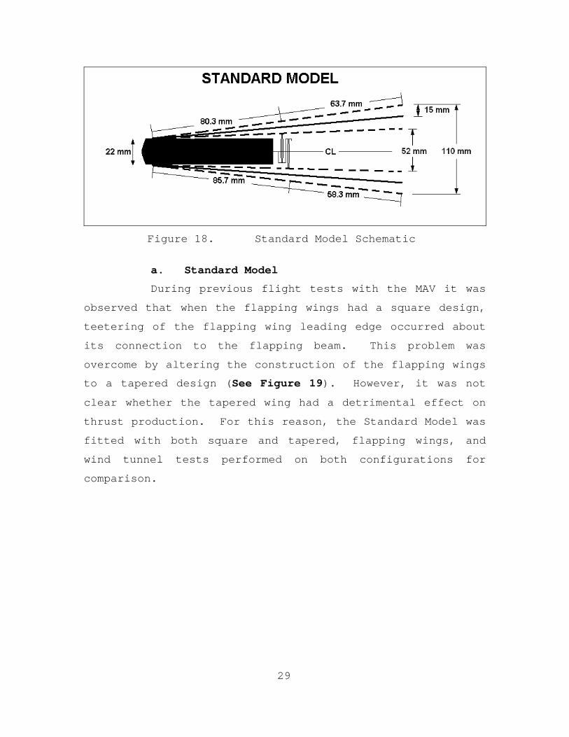
2. Test Geometries

The first test model was built to duplicate as close

as possible the current flying MAV built by Dr. Jones. Key

aspects of its geometry and component materials, except for

the motor and gear system, were identical to the flying

MAV. The plunge amplitude, h, was measured to be 37.5% of

the flapping wing chord. A diagram of this setup can be

seen in Figure 18 and will from here on out be referred to

as the Standard Model.

29

Figure 18. Standard Model Schematic

a. Standard Model

During previous flight tests with the MAV it was

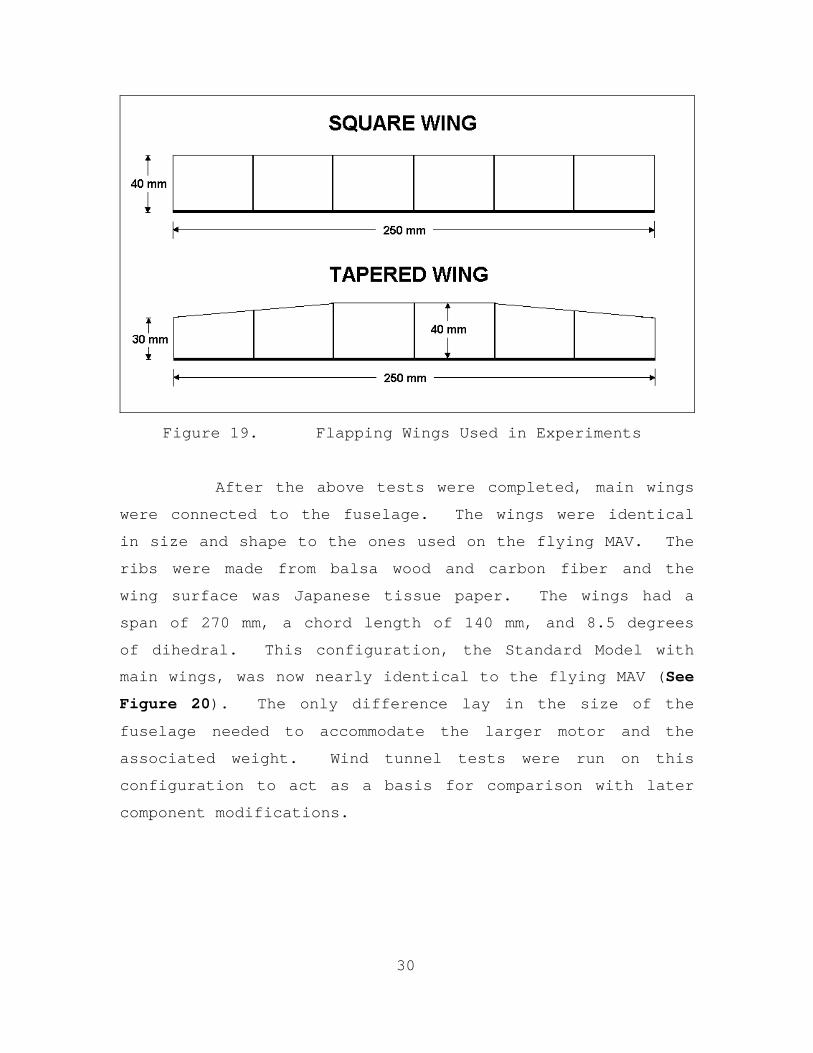
observed that when the flapping wings had a square design,

teetering of the flapping wing leading edge occurred about

its connection to the flapping beam. This problem was

overcome by altering the construction of the flapping wings

to a tapered design (See Figure 19). However, it was not

clear whether the tapered wing had a detrimental effect on

thrust production. For this reason, the Standard Model was

fitted with both square and tapered, flapping wings, and

wind tunnel tests performed on both configurations for

comparison.

30

Figure 19. Flapping Wings Used in Experiments

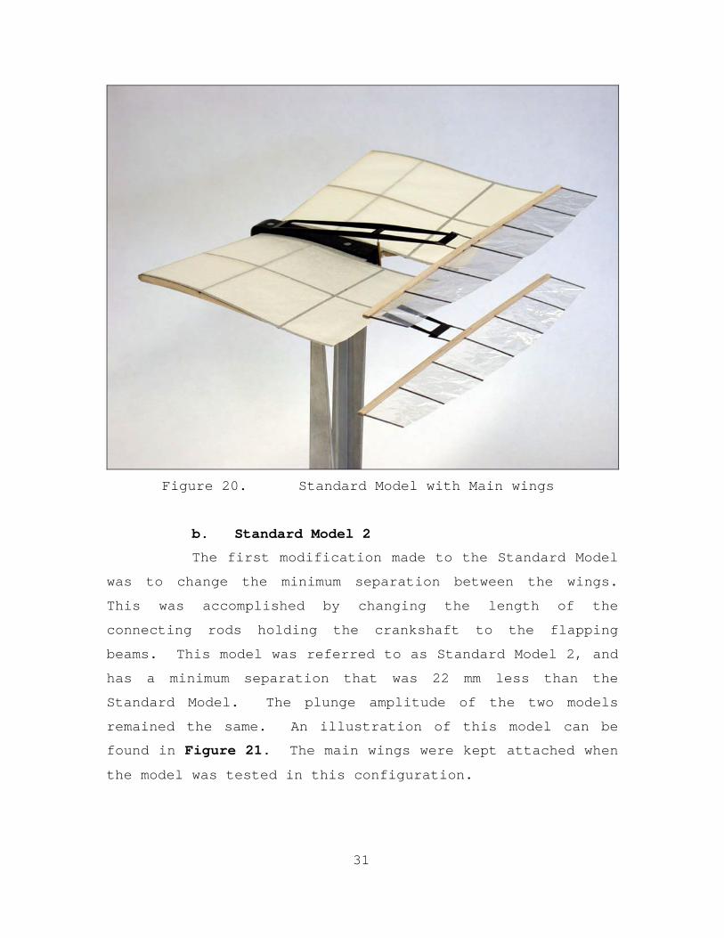
After the above tests were completed, main wings

were connected to the fuselage. The wings were identical

in size and shape to the ones used on the flying MAV. The

ribs were made from balsa wood and carbon fiber and the

wing surface was Japanese tissue paper. The wings had a

span of 270 mm, a chord length of 140 mm, and 8.5 degrees

of dihedral. This configuration, the Standard Model with

main wings, was now nearly identical to the flying MAV (See

Figure 20). The only difference lay in the size of the

fuselage needed to accommodate the larger motor and the

associated weight. Wind tunnel tests were run on this

configuration to act as a basis for comparison with later

component modifications.

31

Figure 20. Standard Model with Main wings

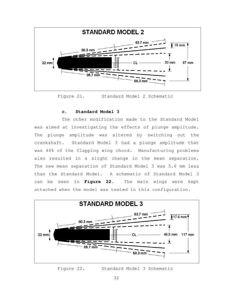
b. Standard Model 2

The first modification made to the Standard Model

was to change the minimum separation between the wings.

This was accomplished by changing the length of the

connecting rods holding the crankshaft to the flapping

beams. This model was referred to as Standard Model 2, and

has a minimum separation that was 22 mm less than the

Standard Model. The plunge amplitude of the two models

remained the same. An illustration of this model can be

found in Figure 21. The main wings were kept attached when

the model was tested in this configuration.

32

Figure 21. Standard Model 2 Schematic

c. Standard Model 3

The other modification made to the Standard Model

was aimed at investigating the effects of plunge amplitude.

The plunge amplitude was altered by switching out the

crankshaft. Standard Model 3 had a plunge amplitude that

was 44% of the flapping wing chord. Manufacturing problems

also resulted in a slight change in the mean separation.

The new mean separation of Standard Model 3 was 5.6 mm less

than the Standard Model. A schematic of Standard Model 3

can be seen in Figure 22. The main wings were kept

attached when the model was tested in this configuration.

Figure 22. Standard Model 3 Schematic

33

C. DATA REDUCTION

1. Cycles

All of the data recorded for the various models was

taken at a sample rate of 2000 HZ for 10 seconds. The data

was analyzed using two MATLAB codes (See Appendix A and B).

The codes were written so that the start and end of each

cycle, as dictated by the square wave input, was found for

each incoming data stream (the data streams being Channels

2, 3, 5 and 6 explained in the experimental setup). The

average value over every cycle was then calculated for that

particular data stream. Next, the mean of all the cycle

averages was found for that sample. Finally, the mean of

the five average sample values for each data set was used

as the final value for that data stream. The standard

deviation of the five mean sample values was used as the

measurement error.

2. Figure of Merit

The figure of merit used to determine the static

performance of the MAV was

PowerShaftThrustofGramsFM = (9)

This is a standard measure of performance used for many

hovering type MAVs. It is important to note that the

numerator in this equation is the thrust available in a

hovering state divided by the acceleration of gravity. For

the NPS MAV the thrust available in a hovering state is the

net positive thrust created by the flapping wings.

3. Error Analysis

The measurements of lift and thrust each contained 4

primary sources of error. From the calibration process the

slope error for both the lift and thrust channels

34

determined by equation (5) was on the order of machine

precision and thus negligible. However, since the

uncertainty of the average values found for each

calibration data set in equation (4) was used to determine

the slope error, this source of error needed to be

included. Another source of uncertainty determined in the

calibration process was the cross-talk between the lift and

thrust channels. This turned out to be approximately 80%

of the total error. One more source of error was the drift

of the load cells during experimentation. Lastly, the

standard deviation for each data set was included in the

calculation for the uncertainty of the data set.

The only source of error involved in the frequency

calculation was the standard deviation of the five average

values found for each data set. This error was found to be

the smallest out of all the measured data. For the worst

case the frequency error was still only 0.2% of the actual

value. Frequency error bars are left off of all subsequent

plots as they are too small to be seen.

The error values calculated for the velocity

measurements account for two uncertainties. The first is

the change in offset from the time the tunnel is turned on

until the time it is turned off. The actual offset used is

the average of these two, but the error is taken as the

full difference between the two data sets. The second

source of error is the drift in velocity from the time the

tunnel speed is set until it is changed again. It is

during this interval that the data sets are recorded.

The uncertainty in the angle of attack is the same for

all conditions and is dependent solely on the resolution of

the angle finder. For these experiments the error was

determined to be +/- 1 degree.

35

a. Error Calculation

The uncertainties listed above for each

measurement were assumed to be independent of one another.

Given this assumption, it is then feasible to calculate the

error using a quadrature technique governed by the equation

⋅⋅⋅+++= 222 zyxerror δδδ (10)

In this equation dx, dy, and dz all represent the

sources of uncertainty in the measurement. Additional

sources of error are added on accordingly.

36

THIS PAGE LEFT INTENTIONALLY BLANK

37

IV. EXPERIMENTAL RESULTS

A. MAV MOTOR

Previous MAV laboratory tests had measured the thrust

production of the NPS MAV to be 9.5 grams using 1.5 Watts

of electrical power. The efficiency of the MAV motor/gear-

drive operating in this region was determined to be

approximately 25% using Figure 17. Neglecting all other

losses in the system other than the motor/gear-drive

efficiency, these numbers provide a MAV Figure of Merit of

25 g/W. All other hovering MAVs currently in production

seem to operate at approximately 10 g/W [Ref. 15]. It can

be clearly seen from these two numbers that the opposed-

plunge, flapping-wing propulsion is much more effective at

producing thrust.

B. STANDARD MODEL

The use of tapered wing shapes to eliminate spanwise

oscillations of the flapping wings was a great aid to the

controllability of the aircraft. It was desired to know

whether this benefit in aircraft control had a detrimental

effect to the thrust produced by the MAV. The MAV thrust

is plotted in Figures 23 and 24 as a function of flapping

frequency for two different AOA and no freestream velocity

using the Standard Model setup.

38

Thrust vs Frequency, Square and Tapered Wings, V = 0m/s

0

0.02

0.04

0.06

0.08

0.1

0.12

9 11 13 15 17 19Frequency (hz)

Thru

st (N

)

0deg AOA; TW 0deg AOA; SW

Figure 23. Thrust vs. Frequency, 0deg AOA, V=0 m/s, SM

Thrust vs Frequency, Square and Tapered Wings, V=0 m/s

00.020.040.060.08

0.10.12

9 11 13 15 17 19 21

Frequency (hz)

Thru

st (N

)

10deg AOA; TW 10deg AOA; SW


Since the error bars overlapped for every data point

in both graphs, and because the square and tapered wings

alternated in each graph as to which was producing more

thrust, it appeared that switching from a square to a

39

tapered flapping wing had a negligible on thrust

production. This was not unreasonable as the amount of

wing area lost due to tapering was only 8.3% of the total

wing area for each wing.

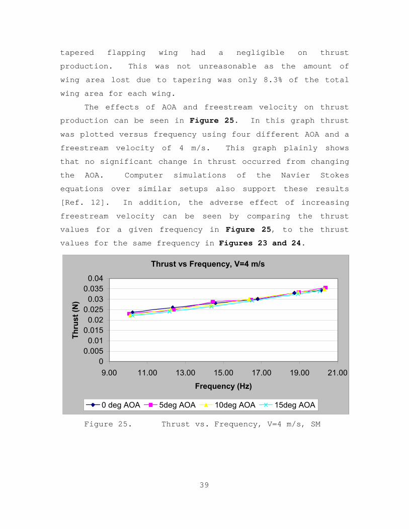
The effects of AOA and freestream velocity on thrust

production can be seen in Figure 25. In this graph thrust

was plotted versus frequency using four different AOA and a

freestream velocity of 4 m/s. This graph plainly shows

that no significant change in thrust occurred from changing

the AOA. Computer simulations of the Navier Stokes

equations over similar setups also support these results

[Ref. 12]. In addition, the adverse effect of increasing

freestream velocity can be seen by comparing the thrust

values for a given frequency in Figure 25, to the thrust

values for the same frequency in Figures 23 and 24.

Thrust vs Frequency, V=4 m/s

00.005

0.010.015

0.020.025

0.030.035

0.04

9.00 11.00 13.00 15.00 17.00 19.00 21.00

Frequency (Hz)

Thru

st (N

)

0 deg AOA 5deg AOA 10deg AOA 15deg AOA

Figure 25. Thrust vs. Frequency, V=4 m/s, SM

40

C. STANDARD MODEL WITH MAIN WINGS

Attaching the main wings seemed to have a slight

negative effect on the thrust being produced by the

flapping wings(See Figure 26 and 27). This could possibly

be a result of the upper flapping wing operating in the

separated flow region behind the upper surface of the

lifting wing. Although the trends on Figure 26 and 27 are

clear, because the error bars overlap the plotted lines,

the statement that the main wings reduce thrust production

can not be claimed for certain.

Thrust vs. Flapping Frequency for V=3m/s

00.010.020.030.040.050.06

9 11 13 15 17 19 21

Frequency (Hz)

Thru

st (N

)

Flapping Wings Only Lifting Wings Figure 26. Thrust vs. Frequency, 0deg AOA, V=3 m/s, SM

41

Thrust vs. Flapping Frequency @ V=3m/s

0

0.01

0.02

0.03

0.04

0.05

0.06

9 11 13 15 17 19 21

Frequency (Hz)

Thru

st (N

)

Flapping Wings Only, 10deg AOA Lifiting Wings, 10deg AOA


D. STANDARD MODEL 2

Decreasing the minimum separation of the wings reduced

the thrust that was produced. This effect can be clearly

seen in Figures 28 and 29. In both of these graphs the

thrust was seen to drop significantly from the Standard

Model.

42

Thrust vs. Frequency for V= 0m/s

00.020.040.060.080.1

0.12

9.00 14.00 19.00 24.00 29.00

Frequency (Hz)

Thru

st (N

SM2, AOA = 0deg SM, AOA = 0deg SM2, AOA = 15deg SM, AOA = 15deg

Figure 28. Thrust vs. Frequency, V=0 m/s, SM2

Thrust vs. Frequency for V = 3 m/s

-0.01

0

0.01

0.02

0.03

0.04

0.05

0.06

9.00 14.00 19.00 24.00 29.00

Frequency (Hz)

Thru

st (N

SM2 = 0deg SM, AOA = 0deg SM2, AOA = 15deg SM, AOA = 15deg

Figure 29. Thrust vs. Frequency, V= 3m/s, SM2

The trailing edges of the flapping wings were seen

to collide with one another at the point of minimum

separation in the flapping cycle. This occurrence seems a

likely explanation for the loss of thrust production seen

in going from the Standard Model to Standard Model 2. The

collision prevented the flapping wings from feathering to

43

their natural positions and reducing the effective angle of

attack. The effective angle of attack is too great without

the feathering phenomenon, and as a result the flow

separates off the flapping-wings and the thrust is

diminished.

Alternatively, the lift was seen to increase

dramatically when reducing the minimum separation (See

Figure 30). The increase in lift was speculated to be a

result of the flow remaining attached over the main wing.

Flow visualization experiments were later conducted to test

this theory. One possible explanation for why the flow

remained attached can be justified by momentum

conservation. If the flapping wings transfer some amount

of momentum to the flow, then this momentum can be used to

either accelerate the freestream to provide thrust, or to

accelerate separated flow to increase lift. This theory

could also account for some of the thrust losses seen in

Figure 29. However, none of these theories can be

substantiated at this juncture.

Lift vs. Frequency for V = 3m/s

-0.0500

0.0000

0.0500

0.1000

0.1500

0.2000

0.2500

9.00 14.00 19.00 24.00 29.00

Frequency (Hz)

Lift

(N)

SM2, AOA = 15deg SM, AOA = 15degSM2, AOA = 5deg SM, AOA = 5deg

Figure 30. Lift vs. Frequency, V=3 m/s, SM2

44

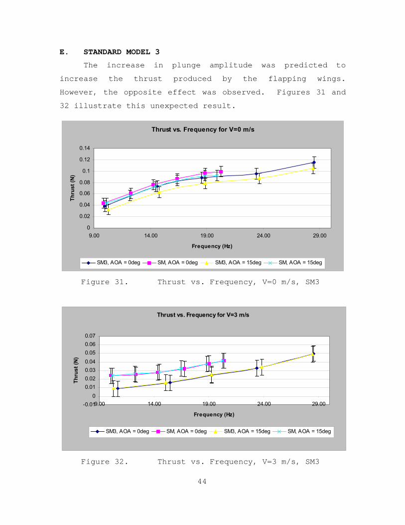
E. STANDARD MODEL 3

The increase in plunge amplitude was predicted to

increase the thrust produced by the flapping wings.

However, the opposite effect was observed. Figures 31 and

32 illustrate this unexpected result.

Thrust vs. Frequency for V=0 m/s

0

0.02

0.04

0.06

0.08

0.1

0.12

0.14

9.00 14.00 19.00 24.00 29.00

Frequency (Hz)

Thru

st (N

)



Thrust vs. Frequency for V=3 m/s

-0.010

0.010.020.030.040.050.060.07

9.00 14.00 19.00 24.00 29.00

Frequency (Hz)

Thru

st (N

)



45

While intuitively it seemed that a greater swept out

area during the flapping cycle would increase thrust, the

elastic effects of the carbon fiber strip connecting the

flapping wings to the flapping beams was not considered.

The tendency of this connection was to allow the wing to

pitch in the direction of the vertical motion in which it

was traveling. Thus, at low freestream velocities such as

in Figure 31, the effective angle of attack was reduced and

a slight drop in performance between Standard Model 3 and

the Standard Model occurred. Conversely, at relatively

fast velocities such as in Figure 32, the elasticity of the

connection acted to increase the effective angle of attack,

inviting separation and the associated loss in thrust.

This phenomenon could also be another possible contribution

to the thrust loss seen in the Standard Model 2

experiments.

Furthermore, the fact that the Standard Model

experiments provided greater amounts of thrust than the

other two models suggested that the desired elasticity of

the carbon-fiber strip changes with the plunge amplitude

and mean separation of the flapping wings. In essence, the

elasticity of the connection was not tuned well with the

rest of the propulsion system for Standard Model 2 and 3,

but was well tuned for the Standard Model. This fact

points to the importance of the elasticity of the carbon

fiber strip connections to the overall performance of the

MAV.

The effects of Standard Model 3 on the lift

performance were somewhat unclear. The lift was found to

dramatically increase with the changes made to this

model(See Figure 33). However, it is unclear whether it

was actually the increased plunge amplitude or the slight

46

reduction in minimum separation that achieved this result.

As before, this improvement in lift was thought to be a

result of the flow remaining attached over the main wing.

Yet once again, the reason for this phenomenon has not yet

been proved.

Lift vs. Frequency for V=3 m/s

-0.0500

0.0000

0.0500

0.1000

0.1500

0.2000

9.00 14.00 19.00 24.00 29.00

Frequency (Hz)

Lift

(N)


Figure 33. Lift vs. Frequency, V=3 m/s, SM3

One unexpected result was the dip in lift seen at the

larger frequencies. This loss of lift was not seen in

either of the other two models, and it is speculated that

vibrations in the outside trailing edge of the main wing

could be responsible (These vibrations were seen in the

flow visualization experiments conducted). The fact that

the drop in lift seems to be associated with frequency

points to the possibility that the problem is related to

damping and again suggests that the propulsion system is

not tuned well for this model.

47

F. FLOW VISUALIZATION

A flow visualization experiment was carried out in

order to confirm that the induced attachment of flow over

the main wing from the flapping wings was the source of the

increased lift seen in Standard Model 2 and 3. Streaklines

were generated upstream of the MAV using a smoke wire and

then recorded with digital video. The pictures presented

here are taken from the digital video frames.

The first test case was the Standard Model. Video was

taken of this model with the flapping on and off at an AOA

of 15 degrees. In Figure 34 one can clearly see that

without any flapping at all the flow separated immediately

after the leading edge.

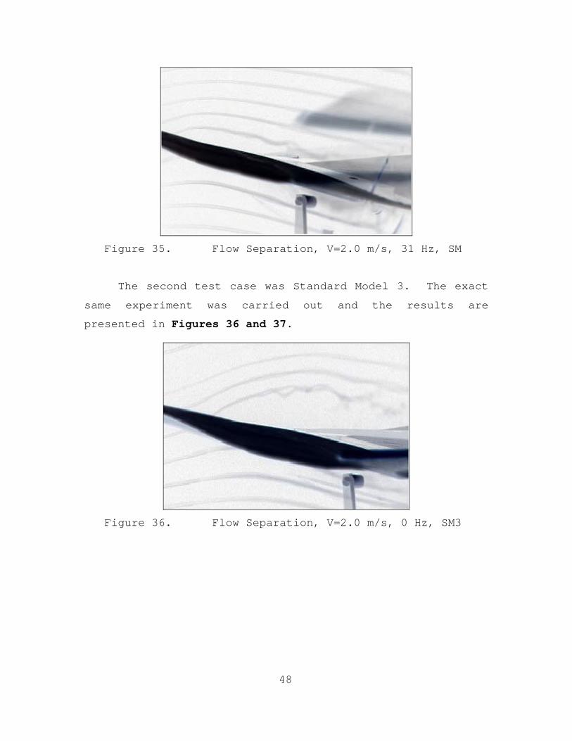
Figure 34. Flow Separation, V=2.0 m/s, 0 Hz, SM

Next, the flapping frequency was set to 31 Hz (See Figure

35). While the separation was not as extreme as in Figure

34, it can clearly be seen that the flow separates before

reaching the end of the main wing.

48

Figure 35. Flow Separation, V=2.0 m/s, 31 Hz, SM

The second test case was Standard Model 3. The exact

same experiment was carried out and the results are

presented in Figures 36 and 37.

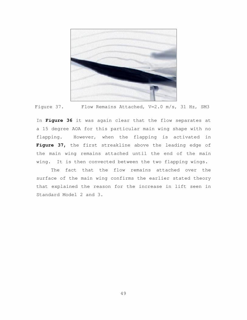
Figure 36. Flow Separation, V=2.0 m/s, 0 Hz, SM3

49

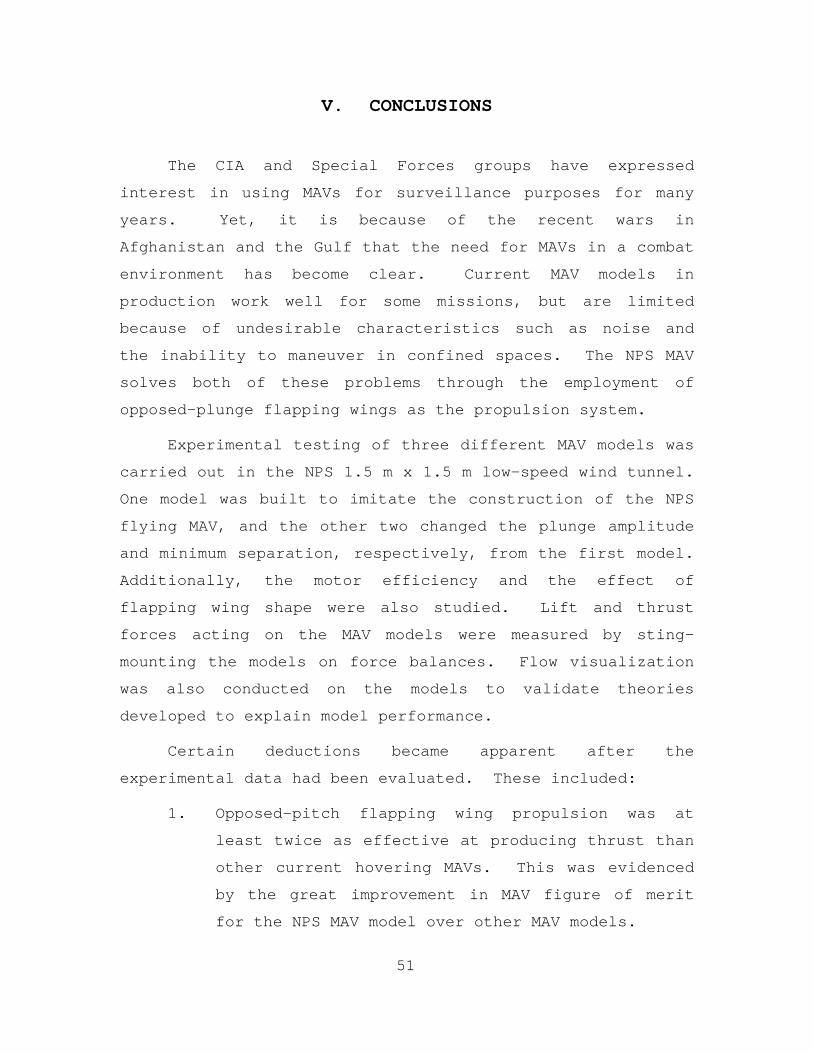
Figure 37. Flow Remains Attached, V=2.0 m/s, 31 Hz, SM3

In Figure 36 it was again clear that the flow separates at

a 15 degree AOA for this particular main wing shape with no

flapping. However, when the flapping is activated in

Figure 37, the first streakline above the leading edge of

the main wing remains attached until the end of the main

wing. It is then convected between the two flapping wings.

The fact that the flow remains attached over the

surface of the main wing confirms the earlier stated theory

that explained the reason for the increase in lift seen in

Standard Model 2 and 3.

50


51

V. CONCLUSIONS

The CIA and Special Forces groups have expressed

interest in using MAVs for surveillance purposes for many

years. Yet, it is because of the recent wars in

Afghanistan and the Gulf that the need for MAVs in a combat

environment has become clear. Current MAV models in

production work well for some missions, but are limited

because of undesirable characteristics such as noise and

the inability to maneuver in confined spaces. The NPS MAV

solves both of these problems through the employment of

opposed-plunge flapping wings as the propulsion system.

Experimental testing of three different MAV models was

carried out in the NPS 1.5 m x 1.5 m low-speed wind tunnel.

One model was built to imitate the construction of the NPS

flying MAV, and the other two changed the plunge amplitude

and minimum separation, respectively, from the first model.

Additionally, the motor efficiency and the effect of

flapping wing shape were also studied. Lift and thrust

forces acting on the MAV models were measured by sting-

mounting the models on force balances. Flow visualization

was also conducted on the models to validate theories

developed to explain model performance.

Certain deductions became apparent after the

experimental data had been evaluated. These included:

1. Opposed-pitch flapping wing propulsion was at

least twice as effective at producing thrust than

other current hovering MAVs. This was evidenced

by the great improvement in MAV figure of merit

for the NPS MAV model over other MAV models.

52

2. The tapered flapping wings used on the NPS MAV

have no measurable effect on thrust production

and reduce spanwise oscillations of the flapping

wings.

3. Thrust was not sensitive to AOA changes between 0

and 15 degrees.

4. Thrust was very sensitive to velocity changes,

with increases in velocity diminishing thrust

production.

5. One possible contribution to the reduced thrust

production seen in Standard Model 2 and 3 is

increased effective angles of attack that are too

great for the flapping wings.

6. The increase in lift seen when mean separation is

reduced can not be definitely attributed to the

decrease in mean separation. Most likely a

secondary effect caused by the reduction in mean

separation is responsible for entraining the

flow.

7. The dramatic increase in lift seen in Standard

Model 2 and 3 as compared with the Standard Model

was a result of inducing the flow to stay

attached over the entire main wing surface. This

theory was confirmed with flow visualization

techniques.

53

VI. RECOMMENDATIONS

The negative effects on thrust production made from

changing the geometric characteristics of the MAV

propulsion system could possibly stem from the elastic

properties of the connection between the flapping wing and

the flapping beam. While this property was not considered

for this paper, undoubtedly the significance of this

parameter has been demonstrated. Perhaps a helpful study

would be to quantify the effects of elasticity on thrust

production as a function of the geometric characteristics

of the MAV propulsion system.

54


55

APPENDIX A. MATLAB CODE FOR CALCULATING EXPERIMENTAL OFFSET VALUES

clear all %BEGIN NESTED FOR LOOP CALCULATIONS; LOAD DATA SETS %USE ZERO SPEED AND ZERO FLAPPING FILE TO SET OFFSETS, THEN USE AT ZERO FLAPPING AT EACH SPPED TO OBTAIN PROFILE DRAG ESTIMATES offset_data = [] for z = 0:4 x = 'load'; eval([x ' ' 'off0100' num2str(z) '.txt']); %INITIALIZE VARIABLES data = zeros(20000,1); data = eval(['off0100' num2str(z)]); lift = zeros(20000,1); lift = data(:,2); thrust = zeros(20000,1); thrust = data(:,3); %FIND AVEGARE VALUES liftavg = 0; liftavg = mean(lift); thrustavg = 0; thrustavg = mean(thrust); %SAVE DATA TO FILE test_data = 0; test_data = [liftavg, thrustavg]; offset_data = [test_data; offset_data]; clear data; clear eval(['off1100' num2str(z)]); end for z = 0:4 x = 'load'; eval([x ' ' 'off0200' num2str(z) '.txt']); %INITIALIZE VARIABLES data = zeros(20000,1); data = eval(['off0200' num2str(z)]); lift = zeros(20000,1); lift = data(:,2); thrust = zeros(20000,1); thrust = data(:,3); %FIND AVEGARE VALUES liftavg = 0; liftavg = mean(lift); thrustavg = 0; thrustavg = mean(thrust); %SAVE DATA TO FILE test_data = 0;

56

test_data = [liftavg, thrustavg]; offset_data = [test_data; offset_data]; clear data; clear eval(['off1200' num2str(z)]); end offsets = mean(offset_data); lift_off = offsets(1) thrust_off = offsets(2)

57

APPENDIX B. MATLAB CODE FOR CALCULATING EXPERIMENTAL THRUST AND LIFT VALUES

clear all LT_offset % INPUT VALUES FROM PRE-FLIGHT ANALYSIS veloccal = 133.2; rhoair = 1.225; velocvolts = 0.0; vinf = ((velocvolts*veloccal)/(0.5*rhoair))^(0.5); b = .250; c = .040; plunge_amp = 0.017625; %VALUES FROM CALIBRATION EXPERIMENTS liftcal = -0.00015651; thrustcal = 5.7349e-005; %BEGIN NESTED FOR LOOP CALCULATIONS; LOAD DATA SETS w = [35,50,63,76,92]; flight_data = [] for yy = 1:5 for zz = 0:4 xx = 'load'; eval([xx ' ' 'pa0' num2str(w(yy)) '00' num2str(zz) '.txt']); %INITIALIZE VARIABLES data = zeros(20000,1); data = eval(['pa0' num2str(w(yy)) '00' num2str(zz)]); lift = zeros(20000,1); lift = (((data(:,2) - lift_off).*liftcal)); thrust = zeros(20000,1); thrust = ((data(:,3) - thrust_off).*thrustcal); %FIND CYCLE START AND END INDICES fbl = 0; fbl = 900; freq = 0; freq = ge(data(:,1),fbl); d = 0; d = find(freq); m = 0; q = 0; [m,q] = size(d); e = zeros(m,1); e(1) = d(1); i = 0; for i = 2:m if [(d(i)-d(i-1)) > 1.5] e(i,1) = d(i); elseif [(d(i)-d(i-1)) == 1]

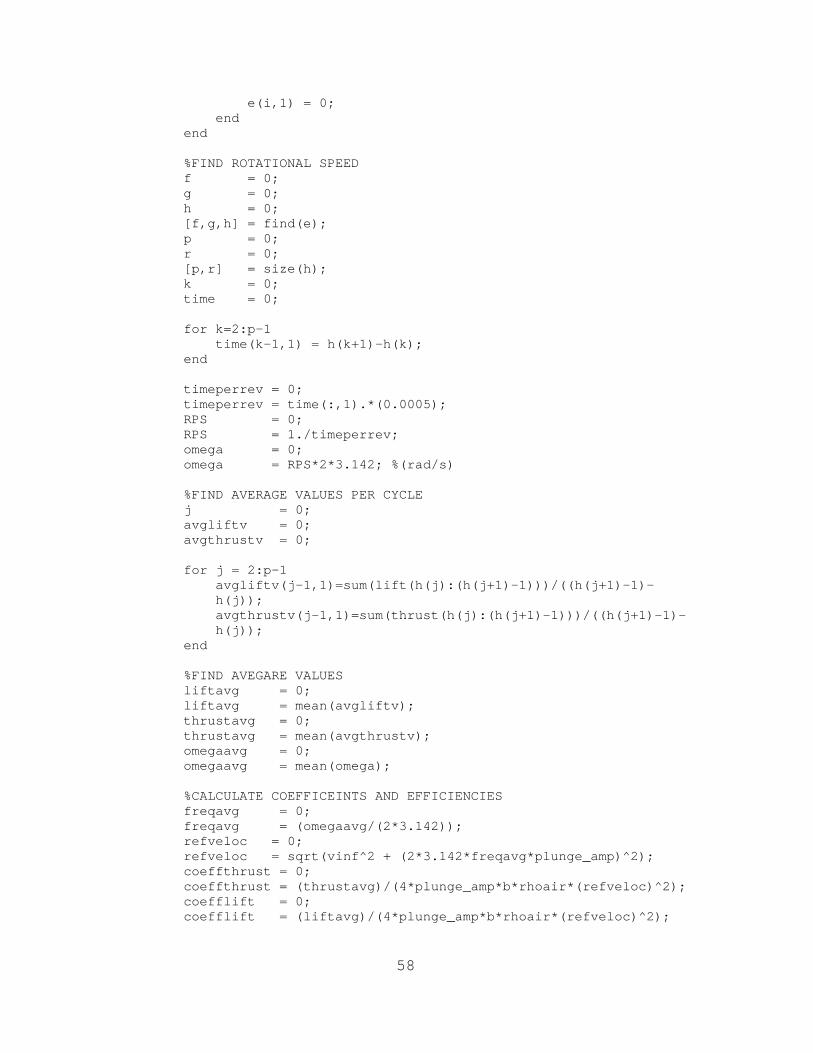
58

e(i,1) = 0; end end %FIND ROTATIONAL SPEED f = 0; g = 0; h = 0; [f,g,h] = find(e); p = 0; r = 0; [p,r] = size(h); k = 0; time = 0; for k=2:p-1 time(k-1,1) = h(k+1)-h(k); end timeperrev = 0; timeperrev = time(:,1).*(0.0005); RPS = 0; RPS = 1./timeperrev; omega = 0; omega = RPS*2*3.142; %(rad/s) %FIND AVERAGE VALUES PER CYCLE j = 0; avgliftv = 0; avgthrustv = 0; for j = 2:p-1 avgliftv(j-1,1)=sum(lift(h(j):(h(j+1)-1)))/((h(j+1)-1)-

h(j)); avgthrustv(j-1,1)=sum(thrust(h(j):(h(j+1)-1)))/((h(j+1)-1)-

h(j)); end %FIND AVEGARE VALUES liftavg = 0; liftavg = mean(avgliftv); thrustavg = 0; thrustavg = mean(avgthrustv); omegaavg = 0; omegaavg = mean(omega); %CALCULATE COEFFICEINTS AND EFFICIENCIES freqavg = 0; freqavg = (omegaavg/(2*3.142)); refveloc = 0; refveloc = sqrt(vinf^2 + (2*3.142*freqavg*plunge_amp)^2); coeffthrust = 0; coeffthrust = (thrustavg)/(4*plunge_amp*b*rhoair*(refveloc)^2); coefflift = 0; coefflift = (liftavg)/(4*plunge_amp*b*rhoair*(refveloc)^2);

59

%SAVE DATA TO FILE test_data = 0; test_data = [freqavg, refveloc, liftavg, thrustavg, coeffthrust, coefflift]; flight_data = [test_data; flight_data]; clear data; clear eval(['ms0' num2str(w(yy)) '00' num2str(zz)]); end end save offset_data offset_data

60


61

APPENDIX C. EXPERIMENTAL DATA FOR STANDARD MODEL WITH LIFTING WINGS

SMLW AOA = 0deg

Freqavg Lift Thrust T_ERROR L_ERRORVinf = 0 m/s 20.26 -0.05102 0.09926 0.00891 0.01972

18.86 -0.05092 0.09586 0.00898 0.01972 16.35 -0.0514 0.0866 0.00903 0.01972 14.24 -0.052 0.07612 0.00900 0.01972 12.26 -0.0542 0.0609 0.00906 0.01976 9.83 -0.05754 0.04386 0.00891 0.01972 Vinf = 1.00 m/s 20.16 -0.04856 0.07966 0.00902 0.01972

18.97 -0.04854 0.07602 0.00896 0.01973 16.45 -0.0495 0.06522 0.00910 0.01972 14.37 -0.0485 0.05272 0.00896 0.01979 12.16 -0.04936 0.03938 0.00896 0.01972 9.99 -0.04864 0.02832 0.00896 0.01975 Vinf = 2.03 m/s 20.39 -0.03376 0.05796 0.00900 0.01972

18.91 -0.03308 0.05248 0.00900 0.01972 16.60 -0.03536 0.04242 0.00900 0.01976 14.70 -0.03518 0.0354 0.00903 0.01973 12.55 -0.03658 0.02758 0.00900 0.01974 10.31 -0.03658 0.02342 0.00900 0.01974 Vinf = 3.00 m/s 20.39 -0.01622 0.04164 0.00890 0.01973

19.01 -0.01538 0.03836 0.00890 0.01974 16.74 -0.02036 0.03218 0.00890 0.01974 14.30 -0.01906 0.02764 0.00891 0.01972 12.30 -0.02242 0.02542 0.00890 0.01974 10.06 -0.02632 0.02394 0.00889 0.01989 Vinf = 4.03 m/s 20.14 -0.00138 0.0343 0.00891 0.02060

18.73 -0.00996 0.033 0.00891 0.01973 16.80 -0.01072 0.0301 0.00892 0.01976 14.57 -0.00982 0.02814 0.00891 0.01973 12.33 -0.00954 0.02598 0.00894 0.01974 10.22 -0.00936 0.02374 0.00891 0.01972 SMLW

AOA = 5deg Freqavg Lift Thrust T_ERROR L_ERROR

Vinf = 0 m/s 20.24 -0.0605 0.09598 0.00901 0.01972 18.69 -0.0656 0.0935 0.00897 0.01972 16.35 -0.0662 0.08466 0.00900 0.01972 14.10 -0.0675 0.07284 0.00897 0.01972 12.11 -0.0678 0.05792 0.00897 0.01973 9.80 -0.0760 0.04264 0.00897 0.01972 Vinf = 1.08 m/s 20.22 -0.0522 0.07892 0.00893 0.01972 18.64 -0.0540 0.0727 0.00892 0.01973 16.54 -0.0568 0.06232 0.00899 0.01972

62

14.40 -0.0588 0.05036 0.00892 0.01973 12.46 -0.0601 0.03866 0.00892 0.01972 10.33 -0.0607 0.02886 0.00892 0.01972 Vinf = 2.06 m/s 20.37 -0.0177 0.05674 0.00890 0.01973 18.71 -0.0191 0.05054 0.00890 0.01975 16.48 -0.0209 0.04304 0.00892 0.01972 14.54 -0.0216 0.03434 0.00891 0.01980 12.04 -0.0263 0.02666 0.00890 0.01972 9.87 -0.0307 0.02348 0.00890 0.01975 Vinf = 3.01 m/s 20.40 0.0155 0.04302 0.00916 0.01973 18.77 0.0191 0.0388 0.00916 0.01975 16.60 0.0157 0.0334 0.00918 0.01986 14.40 0.0146 0.0291 0.00917 0.01974 12.12 0.0105 0.02642 0.00916 0.01972 9.97 0.0097 0.0245 0.00916 0.01973 Vinf = 4.00 m/s 20.37 0.0554 0.03562 0.00910 0.01994

18.97 0.0540 0.03334 0.00912 0.01989 16.46 0.0541 0.0298 0.00914 0.01978 14.45 0.0507 0.02878 0.00911 0.01974 12.39 0.0477 0.02498 0.00944 0.02105 10.04 0.0486 0.02302 0.00911 0.01973 SMLW


Vinf = 0 m/s 20.24 -0.0491 0.09632 0.00890 0.01973 18.57 -0.0500 0.0916 0.00891 0.01972 16.26 -0.0511 0.08442 0.00894 0.01973 14.47 -0.0524 0.0747 0.00890 0.01972 11.92 -0.0568 0.05726 0.00891 0.01973 9.78 -0.0598 0.04196 0.00891 0.01974 Vinf = 0.99 m/s 20.21 -0.0396 0.0833 0.01294 0.02047 18.83 -0.0388 0.07446 0.00891 0.01973 16.54 -0.0388 0.06428 0.00892 0.01972 14.45 -0.0420 0.0573 0.01378 0.02065 12.19 -0.0461 0.04338 0.01379 0.02094 10.01 -0.0450 0.0288 0.00891 0.01972 Vinf = 1.97 m/s 20.01 0.0069 0.05694 0.00915 0.01973

18.80 0.0052 0.05242 0.00915 0.01972 16.55 0.0079 0.04386 0.00917 0.01973 14.39 0.0070 0.03512 0.00915 0.01977 12.13 0.0049 0.0286 0.00915 0.01975 10.24 0.0030 0.02436 0.00915 0.01975 Vinf = 3.05 m/s 20.23 0.0681 0.04224 0.00891 0.01974

18.62 0.0713 0.03816 0.00891 0.01973 16.43 0.0720 0.03222 0.00928 0.01973 14.32 0.0688 0.02886 0.00892 0.01972 12.21 0.0667 0.02596 0.00892 0.01999 10.21 0.0616 0.02402 0.00891 0.01972 Vinf = 4.01 m/s 20.30 0.1408 0.03472 0.00890 0.01974

18.93 0.1331 0.03322 0.00890 0.01988

63

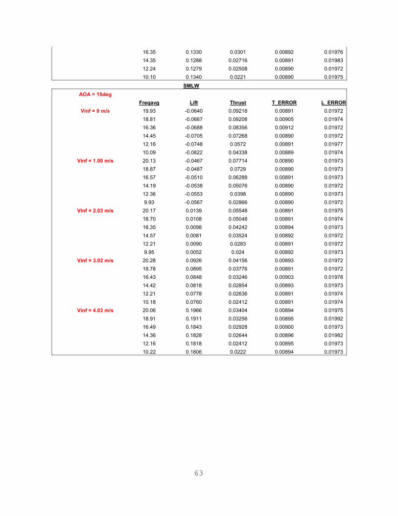
16.35 0.1330 0.0301 0.00892 0.01976 14.35 0.1288 0.02716 0.00891 0.01983 12.24 0.1279 0.02508 0.00890 0.01972 10.10 0.1340 0.0221 0.00890 0.01975 SMLW


Vinf = 0 m/s 19.93 -0.0640 0.09218 0.00891 0.01972 18.81 -0.0667 0.09208 0.00905 0.01974 16.36 -0.0688 0.08356 0.00912 0.01972 14.45 -0.0705 0.07268 0.00890 0.01972 12.16 -0.0748 0.0572 0.00891 0.01977 10.09 -0.0822 0.04338 0.00889 0.01974 Vinf = 1.00 m/s 20.13 -0.0467 0.07714 0.00890 0.01973

18.87 -0.0487 0.0729 0.00890 0.01973 16.57 -0.0510 0.06288 0.00891 0.01973 14.19 -0.0538 0.05076 0.00890 0.01972 12.36 -0.0553 0.0398 0.00890 0.01973 9.93 -0.0567 0.02866 0.00890 0.01972 Vinf = 2.03 m/s 20.17 0.0139 0.05548 0.00891 0.01975

18.70 0.0108 0.05048 0.00891 0.01974 16.35 0.0098 0.04242 0.00894 0.01973 14.57 0.0081 0.03524 0.00892 0.01972 12.21 0.0090 0.0283 0.00891 0.01972 9.95 0.0052 0.024 0.00892 0.01973 Vinf = 3.02 m/s 20.28 0.0926 0.04156 0.00893 0.01972

18.78 0.0895 0.03776 0.00891 0.01972 16.43 0.0848 0.03246 0.00903 0.01978 14.42 0.0818 0.02854 0.00893 0.01973 12.21 0.0778 0.02636 0.00891 0.01974 10.18 0.0760 0.02412 0.00891 0.01974 Vinf = 4.03 m/s 20.06 0.1966 0.03404 0.00894 0.01975

18.91 0.1911 0.03256 0.00895 0.01992 16.49 0.1843 0.02928 0.00900 0.01973 14.36 0.1828 0.02644 0.00896 0.01982 12.16 0.1818 0.02412 0.00895 0.01973 10.22 0.1806 0.0222 0.00894 0.01973

64


65

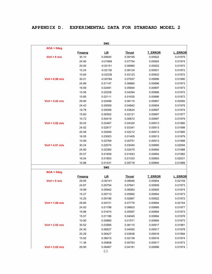
APPENDIX D. EXPERIMENTAL DATA FOR STANDARD MODEL 2

SM2 AOA = 0deg

Freqavg Lift Thrust T_ERROR L_ERRORVinf = 0 m/s 30.10 0.00645 0.09195 0.00922 0.01979

24.90 -0.01668 0.07754 0.00924 0.01974 20.00 -0.02151 0.06960 0.00922 0.01972 15.24 -0.02130 0.06124 0.00931 0.01972 10.60 -0.02238 0.03123 0.00922 0.01972 Vinf = 0.99 m/s 30.01 -0.00784 0.07937 0.00896 0.01990

24.89 0.01147 0.06860 0.00896 0.01973 19.59 0.02481 0.05694 0.00897 0.01973 15.56 0.02208 0.04294 0.00896 0.01972 10.85 0.02111 0.01635 0.00896 0.01972 Vinf = 2.02 m/s 29.90 0.02499 0.06115 0.00897 0.02060

24.43 0.00009 0.04842 0.00904 0.01979 19.78 0.00058 0.03624 0.00897 0.01974 15.60 0.00552 0.02121 0.00897 0.01977 10.72 0.00419 0.00672 0.00897 0.01979 Vinf = 3.02 m/s 30.02 0.02467 0.04320 0.00913 0.01980

24.92 0.02917 0.03341 0.00913 0.01998 20.08 0.02949 0.02212 0.00913 0.01985 16.05 0.03003 0.01405 0.00913 0.01979 10.99 0.02769 0.00751 0.00913 0.01988 Vinf = 4.01 m/s 30.24 0.02074 0.03040 0.00895 0.02094

24.90 0.02360 0.02470 0.00894 0.01988 20.57 0.01659 0.01843 0.00894 0.01982 16.04 0.01803 0.01333 0.00893 0.02031 10.86 0.01431 0.00718 0.00894 0.01989 SM2


Vinf = 0 m/s 29.95 -0.00141 0.08946 0.00904 0.02159 24.87 0.00704 0.07841 0.00909 0.01973 19.99 0.00942 0.06993 0.00905 0.01974 15.27 0.00710 0.05982 0.00904 0.01973 10.25 0.00196 0.02867 0.00922 0.01972 Vinf = 1.00 m/s 29.85 0.04721 0.07776 0.00894 0.02154

24.93 0.01788 0.06603 0.00895 0.01977 19.96 0.01674 0.05597 0.00894 0.01973 15.57 0.01186 0.04045 0.00894 0.01978 10.90 0.00860 0.01571 0.00894 0.01973 Vinf = 2.02 m/s 30.52 0.03585 0.06110 0.00917 0.01981

24.30 0.06527 0.04592 0.00917 0.01978 20.29 0.06427 0.03636 0.00916 0.01994 15.92 0.06015 0.02139 0.00916 0.01974 11.38 0.05808 0.00763 0.00917 0.01973 Vinf = 3.02 m/s 29.90 0.06467 0.04181 0.00896 0.01974

66

24.90 0.06479 0.03240 0.00897 0.01986 20.46 0.06146 0.02288 0.00899 0.01979 16.33 0.05247 0.01468 0.00897 0.01991 10.86 0.04750 0.00773 0.00896 0.01983 Vinf = 4.01 m/s 30.24 0.09382 0.03052 0.00936 0.02025

25.16 0.08349 0.02450 0.00936 0.02121 20.55 0.08228 0.01857 0.00936 0.01978 16.47 0.07747 0.01488 0.00937 0.02030 10.74 0.07565 0.00773 0.00936 0.01998 SM2

AOA = 10deg Freqavg Lift Thrust T_ERROR L_ERRORVinf = 0 m/s 29.95 -0.00832 0.08685 0.00892 0.02642

24.92 0.01345 0.07522 0.00897 0.01974 19.96 0.01595 0.06882 0.00894 0.01973 15.08 0.01237 0.05680 0.00892 0.01975 10.76 0.00556 0.03017 0.00903 0.01973

Vinf = 0.95 m/s 29.85 0.01297 0.07714 0.00905 0.02506 24.70 0.02653 0.06570 0.01059 0.01972 20.21 0.02583 0.05691 0.00905 0.01977 15.46 0.02244 0.04162 0.00905 0.01973 11.07 0.01407 0.01855 0.00905 0.01980

Vinf = 1.99 m/s 30.32 0.10018 0.05982 0.00894 0.01981 24.84 0.10904 0.04832 0.00894 0.01976 20.16 0.10528 0.03663 0.00894 0.01974 15.92 0.10631 0.02219 0.00893 0.01973 11.41 0.10531 0.00818 0.00893 0.01976

Vinf = 3.03 m/s 30.21 0.14465 0.04233 0.00898 0.01973 24.91 0.15400 0.03304 0.00900 0.01975 20.22 0.15029 0.02213 0.00898 0.01972 16.39 0.14759 0.01494 0.00898 0.01974 11.11 0.14785 0.00784 0.00898 0.01981

Vinf = 4.02 m/s 30.13 0.21011 0.03037 0.00890 0.02018 25.29 0.21123 0.02423 0.00891 0.01988 20.71 0.21430 0.01805 0.00891 0.01977 16.32 0.21041 0.01368 0.00890 0.01973 10.89 0.20114 0.00742 0.00890 0.02013

SM2 AOA = 15deg

Freqavg Lift Thrust T_ERROR L_ERRORVinf = 0 m/s 29.90 0.03225 0.08520 0.00898 0.02542

24.97 0.04313 0.07344 0.00898 0.01972 20.12 0.04529 0.06631 0.00896 0.01976 15.38 0.04201 0.05541 0.00891 0.01972 10.48 0.03081 0.02849 0.00892 0.01976 Vinf = 0.94 m/s 30.31 0.01474 0.07668 0.00919 0.02346 25.11 0.02496 0.06389 0.00921 0.01985 20.10 0.01767 0.05507 0.00919 0.01972 15.74 0.01375 0.04039 0.00920 0.01975 10.72 0.00362 0.01500 0.00919 0.01975

67

Vinf = 2.01 m/s 30.38 0.09122 0.05712 0.00899 0.01973 24.88 0.09707 0.04465 0.00901 0.01999 20.02 0.09003 0.03360 0.00898 0.01974 15.87 0.08761 0.02024 0.00898 0.01980 10.87 0.08234 0.00653 0.00898 0.01972

Vinf = 3.0 m/s 30.05 0.17071 0.04224 0.00892 0.01974 24.69 0.18079 0.03431 0.00945 0.01984 20.20 0.17051 0.02231 0.00892 0.01976 16.22 0.16455 0.01434 0.00892 0.01991 10.84 0.15476 0.00884 0.00893 0.01972 Vinf = 3.98 m/s 30.39 0.26620 0.03169 0.00911 0.01988

25.17 0.27513 0.02456 0.00911 0.01989 20.75 0.26442 0.01905 0.00911 0.01989 16.74 0.25625 0.01490 0.00911 0.01974 11.47 0.25180 0.00977 0.00911 0.01976


68

69

APPENDIX E. EXPERIMENTAL DATA FOR STANDARD MODEL 3

SMLW AOA = 0deg

Freqavg Lift Thrust T_ERROR L_ERRORVinf = 0 m/s 20.26 -0.05102 0.09926 0.00891 0.01972

18.86 -0.05092 0.09586 0.00898 0.01972 16.35 -0.0514 0.0866 0.00903 0.01972 14.24 -0.052 0.07612 0.00900 0.01972 12.26 -0.0542 0.0609 0.00906 0.01976 9.83 -0.05754 0.04386 0.00891 0.01972 Vinf = 1.00 m/s 20.16 -0.04856 0.07966 0.00902 0.01972

18.97 -0.04854 0.07602 0.00896 0.01973 16.45 -0.0495 0.06522 0.00910 0.01972 14.37 -0.0485 0.05272 0.00896 0.01979 12.16 -0.04936 0.03938 0.00896 0.01972 9.99 -0.04864 0.02832 0.00896 0.01975 Vinf = 2.03 m/s 20.39 -0.03376 0.05796 0.00900 0.01972

18.91 -0.03308 0.05248 0.00900 0.01972 16.60 -0.03536 0.04242 0.00900 0.01976 14.70 -0.03518 0.0354 0.00903 0.01973 12.55 -0.03658 0.02758 0.00900 0.01974 10.31 -0.03658 0.02342 0.00900 0.01974 Vinf = 3.00 m/s 20.39 -0.01622 0.04164 0.00890 0.01973

19.01 -0.01538 0.03836 0.00890 0.01974 16.74 -0.02036 0.03218 0.00890 0.01974 14.30 -0.01906 0.02764 0.00891 0.01972 12.30 -0.02242 0.02542 0.00890 0.01974 10.06 -0.02632 0.02394 0.00889 0.01989 Vinf = 4.03 m/s 20.14 -0.00138 0.0343 0.00891 0.02060

18.73 -0.00996 0.033 0.00891 0.01973 16.80 -0.01072 0.0301 0.00892 0.01976 14.57 -0.00982 0.02814 0.00891 0.01973 12.33 -0.00954 0.02598 0.00894 0.01974 10.22 -0.00936 0.02374 0.00891 0.01972 SMLW


Vinf = 0 m/s 20.24 -0.06046 0.09598 0.00901 0.01972 18.69 -0.06564 0.09350 0.00897 0.01972 16.35 -0.06620 0.08466 0.00900 0.01972 14.10 -0.06754 0.07284 0.00897 0.01972 12.11 -0.06780 0.05792 0.00897 0.01973 9.80 -0.07598 0.04264 0.00897 0.01972 Vinf = 1.08 m/s 20.22 -0.05218 0.07892 0.00893 0.01972 18.64 -0.05404 0.07270 0.00892 0.01973 16.54 -0.05676 0.06232 0.00899 0.01972 14.40 -0.05876 0.05036 0.00892 0.01973 12.46 -0.06010 0.03866 0.00892 0.01972

70

10.33 -0.06070 0.02886 0.00892 0.01972 Vinf = 2.06 m/s 20.37 -0.01774 0.05674 0.00890 0.01973 18.71 -0.01912 0.05054 0.00890 0.01975 16.48 -0.02094 0.04304 0.00892 0.01972 14.54 -0.02164 0.03434 0.00891 0.01980 12.04 -0.02626 0.02666 0.00890 0.01972 9.87 -0.03068 0.02348 0.00890 0.01975 Vinf = 3.01 m/s 20.40 0.01548 0.04302 0.00916 0.01973 18.77 0.01910 0.03880 0.00916 0.01975 16.60 0.01574 0.03340 0.00918 0.01986 14.40 0.01458 0.02910 0.00917 0.01974 12.12 0.01046 0.02642 0.00916 0.01972 9.97 0.00966 0.02450 0.00916 0.01973 Vinf = 4.00 m/s 20.37 0.05544 0.03562 0.00910 0.01994

18.97 0.05402 0.03334 0.00912 0.01989 16.46 0.05414 0.02980 0.00914 0.01978 14.45 0.05068 0.02878 0.00911 0.01974 12.39 0.04766 0.02498 0.00944 0.02105 10.04 0.04862 0.02302 0.00911 0.01973 SMLW


Vinf = 0 m/s 20.24 -0.04906 0.09632 0.00890 0.01973 18.57 -0.05002 0.09160 0.00891 0.01972 16.26 -0.05112 0.08442 0.00894 0.01973 14.47 -0.05240 0.07470 0.00890 0.01972 11.92 -0.05678 0.05726 0.00891 0.01973 9.78 -0.05978 0.04196 0.00891 0.01974 Vinf = 0.99 m/s 20.21 -0.03964 0.08330 0.01294 0.02047 18.83 -0.03876 0.07446 0.00891 0.01973 16.54 -0.03878 0.06428 0.00892 0.01972 14.45 -0.04196 0.05730 0.01378 0.02065 12.19 -0.04608 0.04338 0.01379 0.02094 10.01 -0.04504 0.02880 0.00891 0.01972 Vinf = 1.97 m/s 20.01 0.00690 0.05694 0.00915 0.01973

18.80 0.00522 0.05242 0.00915 0.01972 16.55 0.00786 0.04386 0.00917 0.01973 14.39 0.00700 0.03512 0.00915 0.01977 12.13 0.00492 0.02860 0.00915 0.01975 10.24 0.00300 0.02436 0.00915 0.01975 Vinf = 3.05 m/s 20.23 0.06810 0.04224 0.00891 0.01974

18.62 0.07128 0.03816 0.00891 0.01973 16.43 0.07204 0.03222 0.00928 0.01973 14.32 0.06880 0.02886 0.00892 0.01972 12.21 0.06668 0.02596 0.00892 0.01999 10.21 0.06156 0.02402 0.00891 0.01972 Vinf = 4.01 m/s 20.30 0.14082 0.03472 0.00890 0.01974

18.93 0.13306 0.03322 0.00890 0.01988 16.35 0.13302 0.03010 0.00892 0.01976 14.35 0.12884 0.02716 0.00891 0.01983

71

12.24 0.12786 0.02508 0.00890 0.01972 10.10 0.13398 0.02210 0.00890 0.01975 SMLW


Vinf = 0 m/s 19.93 -0.06396 0.09218 0.00891 0.01972 18.81 -0.06674 0.09208 0.00905 0.01974 16.36 -0.06876 0.08356 0.00912 0.01972 14.45 -0.07046 0.07268 0.00890 0.01972 12.16 -0.07478 0.05720 0.00891 0.01977 10.09 -0.08218 0.04338 0.00889 0.01974 Vinf = 1.00 m/s 20.13 -0.04666 0.07714 0.00890 0.01973

18.87 -0.04874 0.07290 0.00890 0.01973 16.57 -0.05098 0.06288 0.00891 0.01973 14.19 -0.05378 0.05076 0.00890 0.01972 12.36 -0.05528 0.03980 0.00890 0.01973 9.93 -0.05668 0.02866 0.00890 0.01972 Vinf = 2.03 m/s 20.17 0.01388 0.05548 0.00891 0.01975

18.70 0.01078 0.05048 0.00891 0.01974 16.35 0.00982 0.04242 0.00894 0.01973 14.57 0.00810 0.03524 0.00892 0.01972 12.21 0.00898 0.02830 0.00891 0.01972 9.95 0.00522 0.02400 0.00892 0.01973 Vinf = 3.02 m/s 20.28 0.09256 0.04156 0.00893 0.01972

18.78 0.08950 0.03776 0.00891 0.01972 16.43 0.08480 0.03246 0.00903 0.01978 14.42 0.08182 0.02854 0.00893 0.01973 12.21 0.07776 0.02636 0.00891 0.01974 10.18 0.07600 0.02412 0.00891 0.01974 Vinf = 4.03 m/s 20.06 0.19660 0.03404 0.00894 0.01975

18.91 0.19110 0.03256 0.00895 0.01992 16.49 0.18432 0.02928 0.00900 0.01973 14.36 0.18282 0.02644 0.00896 0.01982 12.16 0.18176 0.02412 0.00895 0.01973 10.22 0.18058 0.02220 0.00894 0.01973


72

73

LIST OF REFERENCES

1. Francis, M.S. and McMichael, J.M., “Micro Air Vehicles - Towards a New Dimension in Flight,” www.darpa.mil/tto/MAV/mav_auvsi.htm, August 7,2002.

2. Grasmeyer, M.J. and Keenon, M.T., “Development of the Black Widow Micro Air Vehicle,” AIAA Paper No. 2001-0127, Simi Valley, California, January 2001.

3. Grossman, J., “The Buzzzz at Caltech, Something New in Southern California’s Skies,” Los Angeles Times Magazine, December 10, 2000, p. 8.

4. Knoller, R., “Die Gesetze des Luftwiderstandes,” Flug-und Motortechnik (Wien), Vol. 3, No. 21, 1909, pp. 1-7.

5. Betz, A., “Ein Beitrag zur Erklarung des Segelfluges,” Zeitschrift fur Flugtechnik und Motorluftschiffahrt, Vol. 3, January. 1912, pp. 269-272.

6. Katzmayr, R., “Effect of Periodic Changes of Angle of Attack on Behavior of Airfoils,” NACA Report No. 147, Oct. 1922 (translated from Zeitschrift fur Flugtechnik und Motorluftschiffart, March 31, 1922, pp.80-82, and April 13, 1922, pp. 95-101).

7. Birnbaum, W., “Das ebene Problem des schlagenden Fluels,” Zeitschrift fur Angewandte Mathematik und Mechanik, Vol. 4, No. 4, August, 1924, pp 277-292.

8. Birnbaum, W., “Der Schlagflugelpropeller und die kleinen Schwingungen elastich befestigter Tragflugel,” Zeitschrift fur Flugtechnik und Motorluftschiffahrt, Vol. 15, 1924, pp. 128-134.

9. Von Karman, T. and Burgers, J.M., “General Aerodynamic Theory – Perfect Fluids,” Division E, Vol. II, Aerodynamic Theory, Ed. Durand, W.F., 1943, p. 308.

74

10. Garrick, I.E., “Propulsion of a Flapping and Oscillating Airfoil,” NACA Report 567, 1936.

11. Schmidt, W., “Der Wellpropeller, ein neuer Antrieb fuer Wasser-, Land-, und Luftfahrzeuge,” Z. Flugwiss. Vol. 13, 1965, pp. 472-479.

12. Jones, K.D., Castro, B.M., Mahmoud, O., and Platzer, M.F., “A Numerical and Experimental Investifation of Flapping Wing Propulsion in Ground Effect,” AIAA Paper No. 2002-0866, Reno, Nevada, January 2002.

13. Jones, K.D., and Platzer, M.F., “Experimental Investigation of the Aerodynamic Characterisitcs of Flapping-Wing Micro Air Vehicles,” AIAA Paper No. 2003-0418, Reno, Nevada, January 2003.

14. Duggan, S.J., An Experimental Investigation of Flapping-Wing Propulsion for Micro Air Vehicles. Master’s Thesis. Naval Postgraduate School. Monterey, California. June 2000.

15. Young, L.A., et. al, “Use of Vertical Lift Planetary

Aerial Vehicles for the Exploration of Mars.” [http://www.lpi.usra.edu/meetings/robomars/pdf/6227. pdf]. June, 2003.

75

INITIAL DISTRIBUTION LIST

1. Defense Technical Information Center Ft. Belvoir, Virginia

2. Dudley Knox Library Naval Postgraduate School Monterey, California

3. Prof. Kevin D. Jones, Code AA/Jo Naval Postgraduate School Monterey, California

4. Prof. Max F. Platzer, Code AA/Pl Naval Postgraduate School Monterey, California 5. Prof. Arthur Schoenstadt

Naval Postgraduate School Monterey, California

6. Ens Jason N. Papadopoulos Naval Postgraduate School Monterey, California

7. Nicholas Papadopoulos

Mary Esther, Florida 8. Ens Jonas B. Kelsall

Seal Team Seven Coronado, California

Documents

An experimental investigation of the geometric ... · The geometric characteristics of flapping-wing propulsion are studied experimentally through ... DARPA’s specifications for