An experimental spatio-temporal model checker?

Vincenzo Ciancia1, Gianluca Grilletti2, Diego Latella1, Michele Loreti3,4, andMieke Massink1

1 Istituto di Scienza e Tecnologie dell’Informazione ‘A. Faedo’, CNR, Pisa, Italy2 Scuola Normale Superiore, Pisa, Italy

3 Universita di Firenze, Italy4 IMT Alti Studi, Lucca, Italy

Abstract. In this work we present a spatial extension of the globalmodel checking algorithm of the temporal logic CTL. This classical veri-fication framework is augmented with ideas coming from the tradition oftopological spatial logics. More precisely, we add to CTL the operators ofthe Spatial Logic of Closure Spaces, including the surrounded operator,with its intended meaning of a point being surrounded by entities sat-isfying a specific property. The interplay of space and time permits oneto define complex spatio-temporal properties. The model checking algo-rithm that we propose features no particular efficiency optimisations, asit is meant to be a reference specification of a family of more efficient al-gorithms that are planned for future work. Its complexity depends on theproduct of temporal states and points of the space. Nevertheless, a pro-totype model checker has been implemented, made available, and usedfor experimentation of the application of spatio-temporal verification inthe field of collective adaptive systems.

1 Introduction

A collective system consists of a large set of interacting individuals. The tempo-ral evolution of the system is not only determined by the decisions taken by theindividuals at the local level, but also by their interactions, that are observableat the global level. By their own nature, such systems feature a “spatial” dis-tribution of the individuals (e.g., locations in physical space, or nodes of somedigital or social network), affecting interaction possibilities and patterns. Verifi-cation of collective systems and of their adaptation mechanisms requires one totake such spatial constraints into account.

In this work, we provide a preliminary study on the feasibility of modelchecking as a fully automated analysis of spatio-temporal models. Our work isgrounded on the so-called snapshot models (see [8] for an introduction). Spatialinformation is encoded by some topological structure, in the tradition of topo-logical spatial logics [10], whereas temporal information is described by a Kripkeframe. The valuation of atomic propositions is a function of temporal states,

? Research partially funded by EU project QUANTICOL (nr. 600708) and IT MIURproject CINA

and spatial locations. We employ Cech closure spaces for the spatial part of themodelling, following the research line initiated in [4] with the definition of theSpatial Logic of Closure Spaces (SLCS). Cech closure spaces are a generalisationof topological spaces also encompassing directed graphs.

Starting from a spatial and a temporal formalism, spatio-temporal logicsmay be defined, by introducing some mutually recursive nesting of spatial andtemporal operators. Several combinations can be obtained, depending on thechosen spatial and temporal fragments, and the permitted forms of nesting ofthe two. A great deal of possibilities are explored in [8], for spatial logics basedon topological spaces. We investigate one such structure, in the setting of closurespaces, namely the combination of the temporal logic Computation Tree Logic(CTL) and of SLCS, resulting in the Spatio-Temporal Logic of Closure Spaces(STLCS). STLCS permits arbitrary mutual nesting of its spatial and temporalfragments. As a proof of concept, we define a simple model checking algorithm,which is a variant of the classical CTL labelling algorithm [5,1], augmented withthe algorithm in [4] for the spatial fragment. The algorithm, which operates onfinite spaces, has been implemented in a prototype tool, available at [7].

Related work. The literature on topological spatial logics is rich (see [11]). How-ever, model checking is typically not taken into account; this is discussed indetail in [4]. In computer science, the term spatial logics has also been used forlogics that predicate about the internal structure of processes in process calculi.A model checker for such kind of logics was developed in [2]. Indeed, the theoryand tool we present are linked to topological spatial logics rather than the areaof process calculi, thus the developed algorithms are very different in nature.

2 Motivating example: adaptive smart transport network

This work is part of a larger research effort aimed at formal verification of spatio-temporal requirements of collective adaptive systems, in the scope of the EU FP7QUANTICOL project5. In order to motivate the proposed tool in the theory ofverification of adaptive systems, we briefly report on a recent case study, detailedin [3], where the STLCS model checker has been used in the context of adaptivesystems, and in particular of smart transport networks. The context is the busnetwork of a city. The model checker is primarily used to identify occurrences ofclumping of buses, that is, buses of the same line that are “too close in space-time” to each other, resulting in several buses of the same line passing by thesame stops within a short amount of time, and longer intervals without any busesat certain stops. More precisely, a bus is part of a clump if it is close to a pointwhere another bus of the same line will be very soon. This statement is inherentlyspatio-temporal, and classical temporal logics do not have the ability to directlyexpress it. It turns out that there is some ambiguity in the formalisation ofthis sentence, resulting in different possible STLCS formulas characterising it.Once established these formulas, the bus coordination system is equipped with an

5 See the web site http://www.quanticol.eu

adaptation layer, enabling buses to wait for some time at a stop, in order to avoidthe emergence of clumps at the expenses of some additional delay on the line.The underlying hypothesis is that clumping happens when some buses are forcedto delay (e.g. because of traffic conditions) but the system evolves immediatelyafterwards, in such a way that subsequent buses of the same line do not delay. TheSTLCS model checker is used to define an analysis methodology that estimatesthe impact of adaptation, before deployment, starting from existing traces (logs)of the system. Each trace, in the form of a series of GPS coordinates for each bus,is considered as a deterministic system. For traces featuring clumping (checkedusing the model checker), the expected non-deterministic behaviour of the systemunder the effect of the adaptation layer is then computed as a spatio-temporalmodel, by augmenting the existing trace with the possible “wait” steps of eachbus. The counterexample-generation capabilities of the model checker are finallyused on such Kripke frame to analyse the impact of the adaptation, by identifyingnew traces containing wait instructions that correct the problem. By doing this,one is able to check if, and under what conditions, the adaptation strategysucceeds in mitigating or eliminating the clumping problem, and confirm ordisprove (depending on the actual situation) the hypothesis underlying the choiceof the adaptation strategy. For more details on the specific case study, we referthe reader to [3]; in the remainder of the paper, we shall focus on the formaldefinition of the STLCS logic, and its model checking algorithm, as both werenot presented in [3].

3 Closure spaces

In this work, we use closure spaces to define basic concepts of space. Below, werecall several definitions, most of which are explained in [6]. See also [4] for athorough description of SLCS, the spatial logic of closure spaces, and its model-checking algorithm. A closure space is a set equipped with a closure operatorobeying to certain laws. In the finite case, closure spaces are graphs, but also(infinite) topological spaces are an instance of the more general constructions.

Definition 1. A closure space is a pair (X, C) where X is a set, and the closureoperator C : 2X → 2X assigns to each subset of X its closure, obeying to thefollowing laws, for all A,B ⊆ X:

1. C(∅) = ∅;2. A ⊆ C(A);3. C(A ∪B) = C(A) ∪ C(B).

The notion of interior, dual to closure, is defined as I(A) = X \ C(X \ A).Closure spaces are a generalisation of topological spaces. The axioms defininga closure space are also part of the definition of a Kuratowski closure space,which is one of the possible alternative definitions of a topological space. Moreprecisely, a topological space is a closure space where the axiom C(C(A)) = C(A)(idempotency) holds. We refer the reader to, e.g., [6] for more information.

Various notions of boundary can be defined. The closure boundary (oftencalled frontier) is used for the surrounded operator in STLCS.

Definition 2. In a closure space (X, C), the boundary of A ⊆ X is definedas B(A) = C(A) \ I(A). The interior boundary is B−(A) = A \ I(A), and theclosure boundary is B+(A) = C(A) \A.

A closure space may be derived starting from a binary relation, that is, a graph.In particular all finite spaces are in this form. This is easily seen by the equivalentcharacterization of quasi-discrete closure spaces.

Definition 3. Consider a set X and a relation R ⊆ X ×X. A closure operatoris obtained from R as CR(A) = A ∪ {x ∈ X | ∃a ∈ A.(a, x) ∈ R}.

Closure spaces derived from a relation can be characterised as quasi-discretespaces (see also Lemma 9 of [6] and the subsequent statements).

Definition 4. A closure space is quasi-discrete if and only if one of the follow-ing equivalent conditions holds: i) each x ∈ X has a minimal neighbourhood6

Nx; ii) for each A ⊆ X, C(A) =⋃a∈A C({a}).

Proposition 1. A closure space (X, C) is quasi-discrete if and only if there isa relation R ⊆ X ×X such that C = CR.

Summing up, a closure space enjoys minimal neighbourhoods, and the closureof A is determined by the closure of the singletons composing A, if and only ifthe space is derived from a relation using Definition 3.

4 The Spatio-Temporal Logic of Closure Spaces

We define a logic interpreted on a variant of Kripke models, where valuationsare interpreted at points of a closure space. Fix a set P of proposition letters.

Definition 5. STLCS formulas are defined by the following grammar, where pranges over P :

Φ ::= > [True]| p [Atomic predicate]| ¬Φ [Not]| Φ ∨ Φ [Or]| N Φ [Close]| ΦS Φ [Surrounded]| Aϕ [All Futures]| Eϕ [Some Future]

ϕ ::= X Φ [Next]| Φ U Φ [Until]

6 A minimal neighbourhood of x is a set A that is a neighbourhood of x, namely,x ∈ I(A), and is included in all other neighbourhoods of x.

The logic STLCS features the CTL path quantifiers A (“for all paths”), andE (“there exists a path”). As in CTL, such quantifiers must necessarily be fol-lowed by one of the path-specific temporal operators, such as7 XΦ (“next”), FΦ(“eventually”), GΦ (“globally”), Φ1 UΦ2 (“until”), but unlike CTL, in this case Φ,Φ1 and Φ2 are STLCS formulas that may make use of spatial operators. Furtheroperators of the logic are the boolean connectives, and the spatial operators NΦ,denoting closeness to points satisfying Φ, and Φ1SΦ2, denoting that a specificpoint satisfying Φ1 is surrounded, via points satisfying Φ1, by points satisfyingΦ2. The mutual nesting of such operators permits one to express spatial proper-ties in which the involved points are constrained to certain temporal behaviours.Let us proceed with a few examples. Consider the STLCS formula EG (green

S blue). This formula is satisfied in a point x in the graph, associated to theinitial state s0, if there exists a (possible) evolution of the system, starting froms0, in which point x, in every state in the path, satisfies green and is surroundedby blue. A further, nested, example is the STLCS formula EF (green S (AX

blue)). This formula is satisfied by a point x in the graph, in the initial states0, if there is a (possible) evolution of the system, starting from s0, in whichpoint x is eventually green and surrounded by points y that, for every possibleevolution of the system from then on, will be blue in the next time step.

A modelM is composed of a Kripke structure (S, T ), where S is a non-emptyset of states, and T is a non-empty accessibility relation on states, and a closurespace (X, C), where X is a set of points and C the closure operator. Every state shas an associated valuation Vs, making ((X, C),Vs) a closure model according toDefinition 6 of [4]. Equivalently, valuations have type S×X → 2P , where P is theset of atomic propositions, thus, the valuation of atomic propositions dependsboth on states and points of the space. Intuitively, there is a set of possible worlds,i.e. the states in S, and a spatial structure represented by a closure space. Ineach possible world there is a different valuation of atomic propositions, inducinga different “snapshot” of the spatial situation which “evolves” over time. In thispaper we assume that the spatial structure (X, C) does not change over time.Other options are indeed possible. For instance, when space depends on S, onemay consider an S-indexed family (Xs, Cs)s∈S of closure spaces.

Definition 6. A model is a structure M = ((X, C), (S, T ),Vs∈S) where (X, C)is a closure space, (S, T ) is a Kripke frame, and V is a family of valuations,indexed by states. For each s ∈ S, we have Vs : P → P(X).

A path in the Kripke structure is a sequence of spatial models (in the senseof [4]) indexed by instants of time; see Fig. 1, where space is a two-dimensionalstructure, and valuations at each state are depicted by different colours.

Definition 7. Given Kripke frame K = (S, T ), a path σ is a function from Nto S such that for all n ∈ N we have (σ(i), σ(i + 1)) ∈ T . Call Ps the set ofinfinite paths in K rooted at s, that is, the set of paths σ with σ(0) = s.

7 Some operators may be derived from others; for this reason, e.g., in Definition 5, andSection 5, we use a minimal set of connectives. As usual in logics, there are severaldifferent choices for such a set.

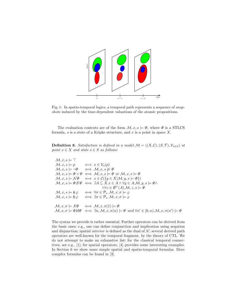
Fig. 1: In spatio-temporal logics, a temporal path represents a sequence of snap-shots induced by the time-dependent valuations of the atomic propositions.

The evaluation contexts are of the form M, x, s |= Φ, where Φ is a STLCSformula, s is a state of a Kripke structure, and x is a point in space X.

Definition 8. Satisfaction is defined in a model M = ((X, C), (S, T ),Vs∈S) atpoint x ∈ X and state s ∈ S as follows:

M, x, s |= >M, x, s |= p ⇐⇒ x ∈ Vs(p)M, x, s |= ¬Φ ⇐⇒ M, x, s 6|= ΦM, x, s |= Φ ∨ Ψ ⇐⇒ M, x, s |= Φ or M, x, s |= ΨM, x, s |= NΦ ⇐⇒ x ∈ C({y ∈ X|M, y, s |= Φ})M, x, s |= ΦS Ψ ⇐⇒ ∃A ⊆ X.x ∈ A ∧ ∀y ∈ A.M, y, s |= Φ∧

∧∀z ∈ B+(A).M, z, s |= ΨM, x, s |= Aϕ ⇐⇒ ∀σ ∈ Ps.M, x, σ |= ϕM, x, s |= Eϕ ⇐⇒ ∃σ ∈ Ps.M, x, σ |= ϕ

M, x, σ |= XΦ ⇐⇒ M, x, σ(1) |= ΦM, x, σ |= ΦUΨ ⇐⇒ ∃n.M, x, σ(n) |= Ψ and ∀n′ ∈ [0, n).M, x, σ(n′) |= Φ

The syntax we provide is rather essential. Further operators can be derived fromthe basic ones; e.g., one can define conjunction and implication using negationand disjunction; spatial interior is defined as the dual of N ; several derived pathoperators are well-known for the temporal fragment, by the theory of CTL. Wedo not attempt to make an exhaustive list; for the classical temporal connec-tives, see e.g., [1]; for spatial operators, [4] provides some interesting examples.In Section 6 we show some simple spatial and spatio-temporal formulas. Morecomplex formulas can be found in [3].

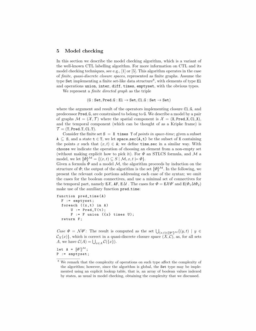
5 Model checking

In this section we describe the model checking algorithm, which is a variant ofthe well-known CTL labelling algorithm. For more information on CTL and itsmodel checking techniques, see e.g., [1] or [5]. This algorithm operates in the caseof finite, quasi-discrete closure spaces, represented as finite graphs. Assume thetype Set implementing a finite set-like data structure8, with elements of type El

and operations union, inter, diff, times, emptyset, with the obvious types.We represent a finite directed graph as the triple

(G : Set, Pred G : El→ Set, Cl G : Set→ Set)

where the argument and result of the operators implementing closure Cl G, andpredecessor Pred G, are constrained to belong to G. We describe a model by a pairof graphs M = (X , T ) where the spatial component is X = (X, Pred X, Cl X),and the temporal component (which can be thought of as a Kripke frame) isT = (T, Pred T, Cl T).

Consider the finite set S = X times T of points in space-time; given a subsetA ⊆ S, and a state t ∈ T, we let space sec(A,t) be the subset of X containingthe points x such that (x, t) ∈ A; we define time sec in a similar way. Withchoose we indicate the operation of choosing an element from a non-empty set(without making explicit how to pick it). For Φ an STLCS formula, and M amodel, we let JΦKM = {(x, t) ⊆ S | M, x, t |= Φ}.Given a formula Φ and a modelM, the algorithm proceeds by induction on thestructure of Φ; the output of the algorithm is the set JΦKM. In the following, wepresent the relevant code portions addressing each case of the syntax; we omitthe cases for the boolean connectives, and use a minimal set of connectives forthe temporal part, namely EX , AF, E U . The cases for Φ = EXΦ′ and E(Φ1 UΦ2)make use of the auxiliary function pred time:

function pred_time(A)

F := emptyset;

foreach ((x,t) in A)

U := Pred_T(t);

F := F union ({x} times U);

return F;

Case Φ = NΦ′: The result is computed as the set⋃

(x,t)∈JΦ′KM{(y, t) | y ∈CX(x)}, which is correct in a quasi-discrete closure space (X, C), as, for all setsA, we have C(A) =

⋃x∈A C({x}).

let A = JΦ′KM;

P := emptyset;

8 We remark that the complexity of operations on such type affect the complexity ofthe algorithm; however, since the algorithm is global, the Set type may be imple-mented using an explicit lookup table, that is, an array of boolean values indexedby states, as usual in model checking, obtaining the complexity that we discussed.

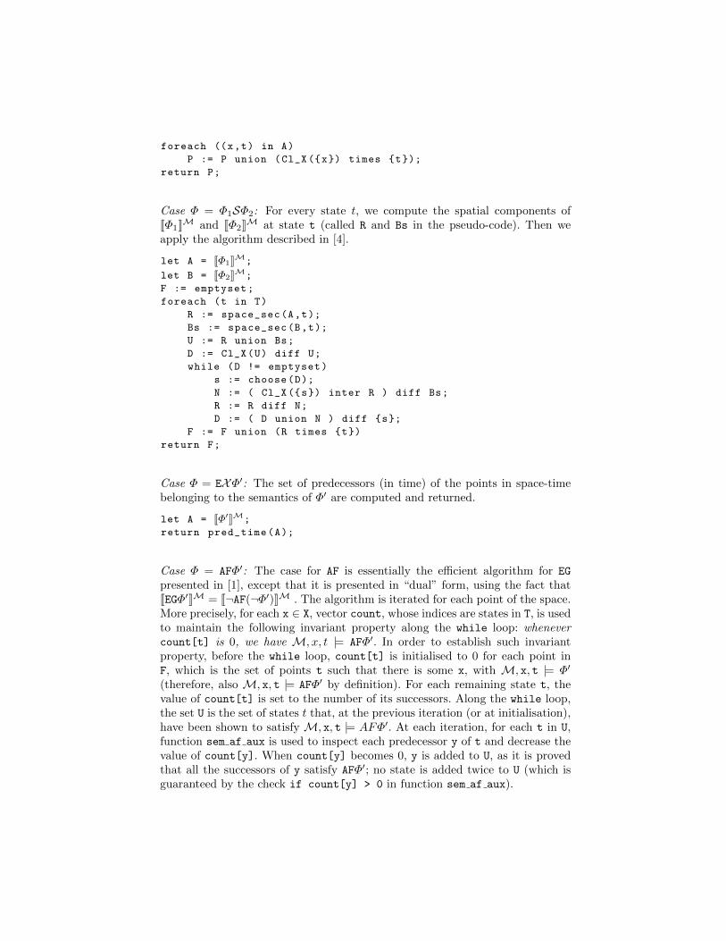
foreach ((x,t) in A)

P := P union (Cl_X({x}) times {t});

return P;

Case Φ = Φ1SΦ2: For every state t, we compute the spatial components ofJΦ1KM and JΦ2KM at state t (called R and Bs in the pseudo-code). Then weapply the algorithm described in [4].

let A = JΦ1KM;

let B = JΦ2KM;

F := emptyset;

foreach (t in T)

R := space_sec(A,t);

Bs := space_sec(B,t);

U := R union Bs;

D := Cl_X(U) diff U;

while (D != emptyset)

s := choose(D);

N := ( Cl_X({s}) inter R ) diff Bs;

R := R diff N;

D := ( D union N ) diff {s};

F := F union (R times {t})

return F;

Case Φ = EXΦ′: The set of predecessors (in time) of the points in space-timebelonging to the semantics of Φ′ are computed and returned.

let A = JΦ′KM;

return pred_time(A);

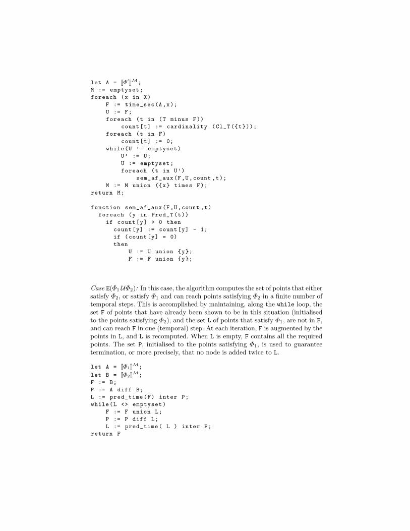
Case Φ = AFΦ′: The case for AF is essentially the efficient algorithm for EG

presented in [1], except that it is presented in “dual” form, using the fact thatJEGΦ′KM = J¬AF(¬Φ′)KM . The algorithm is iterated for each point of the space.More precisely, for each x ∈ X, vector count, whose indices are states in T, is usedto maintain the following invariant property along the while loop: whenevercount[t] is 0, we have M, x, t |= AFΦ′. In order to establish such invariantproperty, before the while loop, count[t] is initialised to 0 for each point inF, which is the set of points t such that there is some x, with M, x, t |= Φ′

(therefore, also M, x, t |= AFΦ′ by definition). For each remaining state t, thevalue of count[t] is set to the number of its successors. Along the while loop,the set U is the set of states t that, at the previous iteration (or at initialisation),have been shown to satisfy M, x, t |= AFΦ′. At each iteration, for each t in U,function sem af aux is used to inspect each predecessor y of t and decrease thevalue of count[y]. When count[y] becomes 0, y is added to U, as it is provedthat all the successors of y satisfy AFΦ′; no state is added twice to U (which isguaranteed by the check if count[y] > 0 in function sem af aux).

let A = JΦ′KM;

M := emptyset;

foreach (x in X)

F := time_sec(A,x);

U := F;

foreach (t in (T minus F))

count[t] := cardinality (Cl_T({t}));

foreach (t in F)

count[t] := 0;

while(U != emptyset)

U’ := U;

U := emptyset;

foreach (t in U’)

sem_af_aux(F,U,count ,t);

M := M union ({x} times F);

return M;

function sem_af_aux(F,U,count ,t)

foreach (y in Pred_T(t))

if count[y] > 0 then

count[y] := count[y] - 1;

if (count[y] = 0)

then

U := U union {y};

F := F union {y};

Case E(Φ1 UΦ2): In this case, the algorithm computes the set of points that eithersatisfy Φ2, or satisfy Φ1 and can reach points satisfying Φ2 in a finite number oftemporal steps. This is accomplished by maintaining, along the while loop, theset F of points that have already been shown to be in this situation (initialisedto the points satisfying Φ2), and the set L of points that satisfy Φ1, are not in F,and can reach F in one (temporal) step. At each iteration, F is augmented by thepoints in L, and L is recomputed. When L is empty, F contains all the requiredpoints. The set P, initialised to the points satisfying Φ1, is used to guaranteetermination, or more precisely, that no node is added twice to L.

let A = JΦ1KM;

let B = JΦ2KM;

F := B;

P := A diff B;

L := pred_time(F) inter P;

while(L <> emptyset)

F := F union L;

P := P diff L;

L := pred_time( L ) inter P;

return F

In the implementation, available at [7], the definition of the Kripke structureis given by a file containing a graph, in the plain text graph description language9

dot. Quasi-discrete closure models are provided either in the form of a graph, orin the form of a set of images, one for each state in the Kripke structure, havingthe same size. The colours of the pixels in the image are the valuation function,and atomic propositions actually are colour ranges for the red, green, and bluecomponents of the colour of each pixel. In this case, the model checker verifies aspecial kind of closure spaces, namely finite regular grids.

The model checker interactively displays the image corresponding to a “cur-rent” state. The most important command of the tool is sem colour formula ,that changes the colour of points satisfying the given formula, to the specifiedcolour, in the current state. The tool has the ability to define parametrisednames for formulas (no recursion is allowed). Formulas are automatically savedand restored from a text file. The implementation is that of a so-called “global”model checker, that is, all points in space-time satisfying the given formulas arecoloured/returned at once. More information on the tool, as well as the completesource code, is available at [7].

The complexity of the currently implemented algorithm is linear in the prod-uct of number of states, subformulas, and points of the space, which is a con-sequence of the algorithm described in [4] being linear in the number of points,and the classical algorithm for CTL being linear in the number of states (in bothcases, for each specific formula). Such efficiency is sufficient for experimentingwith the logic (see [3]), but if both the space and the Kripke structures are large,model checking may become impractical.

Remark 1. Even though we consider a thorough performance analysis of the ba-sic algorithm beyond the scope of this preliminary investigation, and possiblyredundant, we can provide some hints about the feasibility and the efficiencyproblems of spatio-temporal model checking. Our prototype has been imple-mented in OCaml, trying to make use of the declarative features of the lan-guage. For example, we use the Set module of OCaml, implementing a purelyfunctional data type for sets, in order to make use of Definition 8 directly, ratherthan attempting to use bit arrays to improve performance, as it is typical inglobal model checking. In the example of Section 2, we considered rather smallKripke frames, in the order of one hundred states. However, the images associ-ated to each state contain around one million points. Therefore, even though thestate space seems rather small, the number of examined points in space-time isin the order of 50-100 millions of states. The model checker is able to performthe required analyses in a time that roughly varies between some seconds and 30minutes, depending on the formula, on a quite standard laptop computer. On theone hand, this proves that non-trivial examples may be analysed using the simplealgorithm we proposed, but on the other hand, the same data strongly suggeststhat effective optimisations need to be found to make large-scale spatio-temporalmodel checking feasible (more on this in the conclusions).

9 Further information on the dot notation can, for example, be found athttp://www.graphviz.org/Documentation.php.

6 Examples

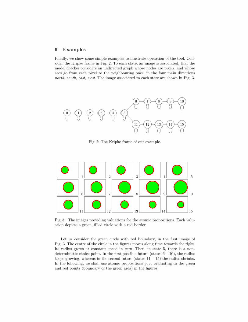
Finally, we show some simple examples to illustrate operation of the tool. Con-sider the Kripke frame in Fig. 2. To each state, an image is associated, that themodel checker considers an undirected graph whose nodes are pixels, and whosearcs go from each pixel to the neighbouring ones, in the four main directionsnorth, south, east, west. The image associated to each state are shown in Fig. 3.

0 1 2 3 4 5

6 7 8 9 10

11 12 13 14 15

Fig. 2: The Kripke frame of our example.

1 2 3 4 5

6 7 8 9 10

11 12 13 14 15

Fig. 3: The images providing valuations for the atomic propositions. Each valu-ation depicts a green, filled circle with a red border.

Let us consider the green circle with red boundary, in the first image ofFig. 3. The centre of the circle in the figures moves along time towards the right.Its radius grows at constant speed in turn. Then, in state 5, there is a non-deterministic choice point. In the first possible future (states 6− 10), the radiuskeeps growing, whereas in the second future (states 11− 15) the radius shrinks.In the following, we shall use atomic propositions g, r, evaluating to the greenand red points (boundary of the green area) in the figures.

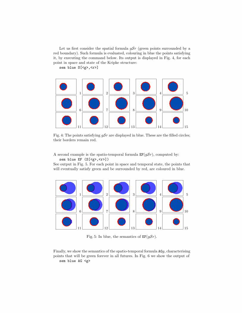
Let us first consider the spatial formula gSr (green points surrounded by ared boundary). Such formula is evaluated, colouring in blue the points satisfyingit, by executing the command below. Its output is displayed in Fig. 4, for eachpoint in space and state of the Kripke structure:

sem blue S[<g>,<r>]

1 2 3 4 5

6 7 8 9 10

11 12 13 14 15

Fig. 4: The points satisfying gSr are displayed in blue. These are the filled circles;their borders remain red.

A second example is the spatio-temporal formula EF(gSr), computed by:sem blue EF (S[<g>,<r>])

See output in Fig. 5. For each point in space and temporal state, the points thatwill eventually satisfy green and be surrounded by red, are coloured in blue.

1 2 3 4 5

6 7 8 9 10

11 12 13 14 15

Fig. 5: In blue, the semantics of EF(gSr).

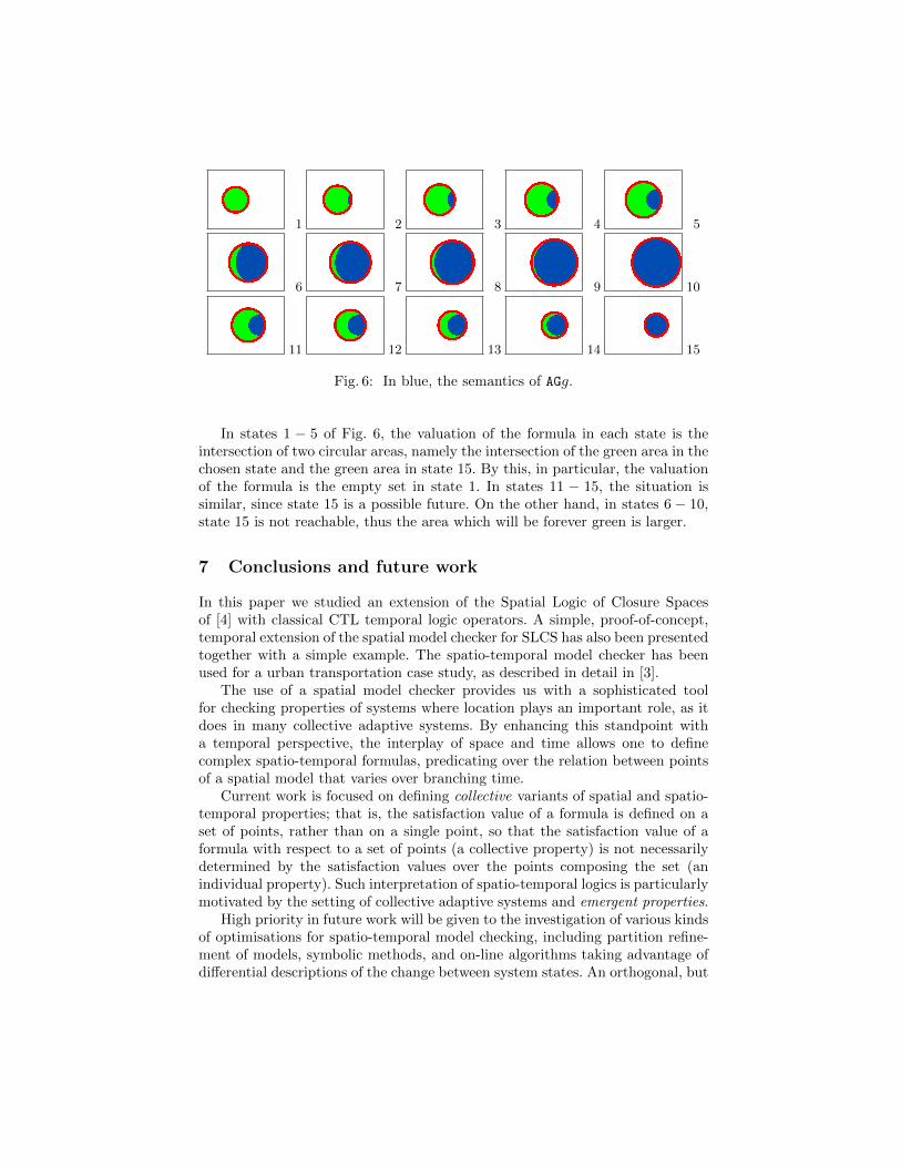
Finally, we show the semantics of the spatio-temporal formula AGg, characterisingpoints that will be green forever in all futures. In Fig. 6 we show the output of

sem blue AG <g>

1 2 3 4 5

6 7 8 9 10

11 12 13 14 15

Fig. 6: In blue, the semantics of AGg.

In states 1 − 5 of Fig. 6, the valuation of the formula in each state is theintersection of two circular areas, namely the intersection of the green area in thechosen state and the green area in state 15. By this, in particular, the valuationof the formula is the empty set in state 1. In states 11 − 15, the situation issimilar, since state 15 is a possible future. On the other hand, in states 6 − 10,state 15 is not reachable, thus the area which will be forever green is larger.

7 Conclusions and future work

In this paper we studied an extension of the Spatial Logic of Closure Spacesof [4] with classical CTL temporal logic operators. A simple, proof-of-concept,temporal extension of the spatial model checker for SLCS has also been presentedtogether with a simple example. The spatio-temporal model checker has beenused for a urban transportation case study, as described in detail in [3].

The use of a spatial model checker provides us with a sophisticated toolfor checking properties of systems where location plays an important role, as itdoes in many collective adaptive systems. By enhancing this standpoint witha temporal perspective, the interplay of space and time allows one to definecomplex spatio-temporal formulas, predicating over the relation between pointsof a spatial model that varies over branching time.

Current work is focused on defining collective variants of spatial and spatio-temporal properties; that is, the satisfaction value of a formula is defined on aset of points, rather than on a single point, so that the satisfaction value of aformula with respect to a set of points (a collective property) is not necessarilydetermined by the satisfaction values over the points composing the set (anindividual property). Such interpretation of spatio-temporal logics is particularlymotivated by the setting of collective adaptive systems and emergent properties.

High priority in future work will be given to the investigation of various kindsof optimisations for spatio-temporal model checking, including partition refine-ment of models, symbolic methods, and on-line algorithms taking advantage ofdifferential descriptions of the change between system states. An orthogonal, but

nevertheless interesting, aspect of spatio-temporal computation is the introduc-tion of probability and stochastic aspects, as well as the introduction of metrics,yielding bounded versions of the introduced spatio-temporal connectives. Suchfeatures will be studied in the context of STLCS. Investigating efficient modelchecking algorithms in this setting is important for practical applications, whichare very often quantitative rather than boolean.

Another ongoing work is the development of qualitative and quantitativespatio-temporal analysis of the behaviour of complex systems, which was startedin [9], and features an extension of Signal Temporal Logic to accommodate spa-tial information. In that case, models are deterministic (thus non-branching)and monitoring plays a central role. Single, infinite traces (intended to be theoutcome of some approximation of a complex sytem, described by a system ofdifferential equations) are analysed to check whether specific spatio-temporalproperties are satisfied, such as, the formation of specific patterns.

References

1. C. Baier and J. P. Katoen. Principles of model checking. MIT Press, 2008.2. Luıs Caires and Hugo Torres Vieira. SLMC: A tool for model checking concurrent

systems against dynamical spatial logic specifications. In Cormac Flanagan andBarbara Konig, editors, Tools and Algorithms for the Construction and Analysisof Systems - 18th International Conference, TACAS 2012, volume 7214 of LectureNotes in Computer Science, pages 485–491. Springer, 2012.

3. V. Ciancia, S. Gilmore, G. Grilletti, D. Latella, M. Loreti, and M. Massink. Spatio-temporal model-checking of vehicular movement in transport systems. submittedfor journal publication, available from the authors.

4. V. Ciancia, D. Latella, M. Loreti, and M. Massink. Specifying and Verifying Prop-erties of Space. In Springer, editor, The 8th IFIP International Conference onTheoretical Computer Science, TCS 2014, Track B, volume 8705 of Lecture Notesin Computer Science, pages 222–235, 2014.

5. E. M. Clarke, O. Grumberg, and D. Peled. Model checking. MIT Press, 2001.6. A. Galton. A generalized topological view of motion in discrete space. Theoretical

Computer Science, 305(1–3):111 – 134, 2003.7. G. Grilletti and V. Ciancia. STLCS model checker, 2014. https://github.com/

cherosene/ctl_logic.8. R. Kontchakov, A. Kurucz, F. Wolter, and M. Zakharyaschev. Spatial logic +

temporal logic = ? In M. Aiello, I. Pratt-Hartmann, and J. van Benthem, editors,Handbook of Spatial Logics, pages 497–564. Springer, 2007.

9. L. Nenzi, L. Bortolussi, V. Ciancia, M. Loreti, and M. Massink. Qualitative andquantitative monitoring of spatio-temporal properties. submitted.

10. J. van Benthem and G. Bezhanishvili. Modal logics of space. In M. Aiello, I. Pratt-Hartmann, and J. van Benthem, editors, Handbook of Spatial Logics, pages 217–298.Springer, 2007.

11. J. van Benthem and G. Bezhanishvili. Modal logics of space. In Handbook ofSpatial Logics, pages 217–298. 2007.