An Experimental Study of a Simple, Distributed Edge-Coloring Algorithm

An Experimental Study of a Simple,Distributed Edge-Coloring Algorithm

MADHAV V. MARATHELos Alamos National LaboratoryALESSANDRO PANCONESIUniversita La Sapienza di RomaandLARRY D. RISINGER JRLos Alamos National Laboratory

We conduct an experimental analysis of a distributed randomized algorithm for edge coloring simpleundirected graphs. The algorithm is extremely simple yet, according to the probabilistic analysis, itcomputes nearly optimal colorings very quickly [Grable and Panconesi 1997]. We test the algorithmon a number of random as well as nonrandom graph families.

The test cases were chosen based on two objectives: (i) to provide insights into the worst-casebehavior (in terms of time and quality) of the algorithm and (ii) to test the performance of thealgorithm with instances that are likely to arise in practice. Our main results include the following:

(1) The empirical results obtained compare very well with the recent empirical results reportedby other researchers [Durand et al. 1994, 1998; Jain and Werth 1995].

(2) The empirical results confirm the bounds on the running time and the solution quality asclaimed in the theoretical paper. Our results show that for certain classes of graphs the algo-rithm is likely to perform much better than the analysis suggests.

(3) The results demonstrate that the algorithm might be well suited (from a theoretical as well aspractical standpoint) for edge coloring graphs quickly and efficiently in a distributed setting.

Based on our empirical study, we propose a simple modification of the original algorithm withsubstantially improved performance in practice.Additional Key Words and Phrases: Distributed algorithms, edge coloring, experimental analysisof algorithms, high performance computing, randomized algorithms, scheduling.

The work is supported by the Department of Energy under Contract W-7405-ENG-36, the ASCIinitiative and the DOE AMS program. “An experimental study of a simple, distributed edge coloringalgorithm,” appeared in Proc. of 12th ACM Symposium on Parallel Algorithms and Architectures(SPAA), 2000, pp. 166–175.Authors’ addresses: Madhav V. Marathe, Basic and Applied Simulation Science (CCS-5), P.O. Box1663, MS M997, Los Alamos National Laboratory, Los Alamos NM 87545; email: [email protected];Alessandro Panconesi, Dipartimento di Informatica, Universita La Sapienza di Roma, via Salaria113, 00198 Roma Italy. Most of the work was done while at BRICS, University of Århus, DK-8000Århus C, Denmark; email: [email protected]; Larry D. Risinger jr, ISR5, Los Alamos NationalLaboratory, P.O. Box 1663, MS J570 Los Alamos NM 87545. email: [email protected] to make digital or hard copies of part or all of this work for personal or classroom use isgranted without fee provided that copies are not made or distributed for profit or direct commercialadvantage and that copies show this notice on the first page or initial screen of a display alongwith the full citation. Copyrights for components of this work owned by others than ACM must behonored. Abstracting with credit is permitted. To copy otherwise, to republish, to post on servers,to redistribute to lists, or to use any component of this work in other works requires prior specificpermission and/or a fee. Permissions may be requested from Publications Dept., ACM, Inc., 1515Broadway, New York, NY 10036 USA, fax: +1 (212) 869-0481, or [email protected]© 2004 ACM 1084-6654/04/0001-ART01 $5.00

ACM Journal of Experimental Algorithmics, Vol. 9, Article No. 1.3, 2004, Pages 1–22.

2 • M. V. Marathe et al.

1. INTRODUCTION AND MOTIVATION

An edge coloring of a graph is an assignment of colors to the edges of the graphsuch that edges incident on the same vertex receive different colors. Equiva-lently, an edge coloring can be viewed as a partition of the edges into disjointmatchings. The minimum number of colors with which the graph G can be col-ored is called the chromatic index of G and is customarily denoted by χ ′(G).In this paper we conduct an experimental study of a very simple distributedalgorithm for the edge-coloring problem. Theoretical analysis [see Grable andPanconesi 1997] shows that this algorithm performs very well asymptotically,that is, it computes nearly optimal edge colorings very quickly. The algorithmcan fail but, according to theoretical analysis, this happens with a probabilitythat tends to 0 as the size of the input graph grows. The experimental analysiswas motivated by certain applications of edge colorings in the context of schedul-ing (see below) and the desirable features of the algorithm (speed, quality, andsimplicity of implementation). Our results show that the algorithm performsreasonably well in practice and might very well be suitable for real applications.

The kind of applications we have in mind are related to the schedulingof data transfers in large parallel architectures. The usefulness of edge col-oring in this context was already noted by several authors. (See Jain et al.[1992b] for a comprehensive survey of applications arising in various ar-eas.) Our original motivation for studying edge-coloring problems was thegather-scatter problem arising in the context of the Telluride project at LosAlamos [Kothe et al. 1997; Ferrell et al. 1997] . See http://www.lanl.gov/asci/and http://public.lanl.gov/mww/HomePage.html for more details about theseprojects.

A similar edge-coloring problem arises in other distributed computing ap-plications [see Jain et al. 1992a, 1992b; Durand et al. 1998, 1994]. In all theseapplications a distributed network is required to compute an edge coloring ofits own unknown topology. As a result, a simple and fast distributed algorithmfor computing near-optimal colorings is preferable to a cumbersome centralizedapproach, even when the latter is able to compute optimal solutions. The rea-sons for this are twofold: (i) the task of finding good schedules for data exchangeshould be a small fraction of total computation time, and (ii) the amount of in-formation that needs to be gathered at a central location will require prohibitiveamounts of resources (e.g., time and memory).

The rest of the paper is organized as follows. Section 2 summarizes our re-sults. Section 3 discusses related work. In Section 4, we describe the algorithmand discuss important implementation aspects. Section 5 provides an intuitiveexplanation of why the algorithm works. This provides a basis for the class ofgraphs on which subsequent empirical analysis is reported. In Section 7, weanalyze our results on various graph classes.

2. SUMMARY OF RESULTS

In this paper, we conduct an experimental analysis of the following random-ized, distributed algorithm (referred to as S).Initially each edge is given a list,or palette, of (1 + ε)� colors, where � is the maximum degree of the network

ACM Journal of Experimental Algorithmics, Vol. 9, Article No. 1.3, 2004.

Distributed Edge Coloring Algorithm • 3

(graph). The computation proceeds in rounds. During each round, each uncol-ored edge, in parallel, first picks a tentative color at random from its palette.If no neighboring edge picks the same color, the color becomes final and thealgorithm stops for that edge. Otherwise, the edge’s palette is updated in theobvious way—the colors successfully used by the neighbors are removed—and anew attempt is performed in the next round. Section 4 discusses the algorithmin greater detail.

Algorithm S is very simple and distributed, yet guarantees that the numberof colors used is a small multiplicative factor of the optimal value, provided themaximum degree of the graph is not “too small” (see discussion below) [Grableand Panconesi 1997].

Here, we conduct an extensive empirical analysis of the algorithm S. Theanalysis is conducted by running the algorithm on a simulated synchronous,message-passing, distributed network environment. Such an environment is atheoretical abstraction of real distributed architectures where typically the costof routing messages is orders of magnitude greater than that of performing localcomputations. In this abstract model of computation, we have a graph whosevertices correspond to processors and whose edges correspond to bidirectionalcommunication links. There is no shared memory. Computation proceeds inrounds. During each round a processor performs some internal computationand exchanges information with the neighbors in the graph. The complexityof the protocol is, by definition, the number of rounds needed to compute theoutput correctly. In our example, this corresponds to a valid edge coloring of thenetwork. In this model, local computation is not charged for, but communicationis. Therefore, the model is somewhat orthogonal to the PRAM model.

We carry out our experimental analysis by simulating this theoretical model,as opposed to running the algorithm on a real parallel architecture, for thefollowing reasons. Our simulation is aimed at ascertaining whether the sim-ple stochastic process (S) described above shows the good behavior predictedby the analysis in real situations. Whereas this simulation is, in terms of re-sources and programming effort, relatively inexpensive, an implementation ona real parallel machine would be much more demanding. Moreover, a trulydistributed implementation would introduce factors that would make the ex-perimental results more informative for the specific applications considered,but probably unsuitable for drawing general conclusions about the behavior ofthe algorithm. There are also other reasons why our approach appears to besound. One obvious problem with experimental studies of algorithms, in gen-eral, is that they are based on a specific implementation on a specific machine.This makes it very hard to compare different experimental results. Thus, it isuseful to find a middle-ground between the world of asymptotics and real im-plementations, which on the one the hand provides accurate predictions on atleast some important aspects of the algorithm, and on the other hand makes itpossible to cleanly compare different experimental results.

For the experimental analysis, we consider (i) graph classes that bring forththe worst-case behavior of the algorithm, and (ii) graph classes that are likelyto arise in practical situation. These are described in detail in the sequel(Section 5).



The input to the algorithm is a graph satisfying a certain condition on themaximum degree (denoted by �) of the graph. A precise statement of this con-dition is deferred to Section 4. Roughly, it says that the maximum degree of thegraph should be high enough. In particular, it should be the case that � � log n,where n is the number of vertices of the input graph ( f (n) � g (n) if f (n)/g (n)tends to infinity as n grows). The palette size—the number of colors that thealgorithm is allowed to use—is also part of the input. In the analysis, we mea-sure how the running time and the failure probability depend on the relevantvariables: palette size, graph size, maximum degree of the graph, and the graphtopology. Specific conclusions obtained as a result of our analysis include thefollowing:

—S’s running time performance is extremely good. The algorithm colors ran-dom graphs with as many as half a million edges in about 10 communicationrounds. For all practical purposes, the number of rounds is unlikely ever toexceed 15.

—In contrast, the failure probability is higher than anticipated and likely tomake the algorithm not very useful. However, the following simple modifi-cation eliminates the problem: If some of the edges run out of colors duringthe course of the algorithm (this is the only way in which the algorithm canfail) they are simply given a few more fresh new colors and the algorithmcontinues as before. This modified algorithm is referred to as algorithm M.Notice that M remains a truly distributed algorithm, for the palette enlarge-ment can be carried out locally. Algorithm M never fails but its performancemust now be measured in terms of both running time and number of colorsactually used. In practice, we found that M remains extremely fast—it neverexceeds 3 or 4 additional rounds—and its color performance is satisfactory(see below).

—As remarked, for the algorithms to work well, the theoretical analysis pre-scribes that the initial degree be “high enough.” Our analysis reveals thatin some cases, this condition is critical (e.g., hypercubes) but in many othercases it can be relaxed.

—The theoretical analysis shows that asymptotically (i.e., for large n) thepalette size can be pushed arbitrarily close to � (and hence to the optimum;recall that χ ′(G) ≥ �(G) for all graphs G). In practice, however, we foundthat a more realistic value for the number of colors used by M is between 5%and 10% greater than �.

In view of the above observations, we expect the algorithms, especially algo-rithm M, to be useful if implemented on real distributed architectures.

3. RELATED WORK

The problem of finding efficient edge-colorings of a graph has been a subject ofactive research over the last three decades. The problem is known to be NP-complete [Hoyler 1980]. Numerous papers have been published on this topic—ranging from near-optimal sequential algorithms to randomized distributedalgorithms. We refer the reader to Hochbaum [1997], Grable and Panconesi



[1997], Panconesi and Srinivasan [1992], Dubhashi et al. [1998], Jain et al.[1992a, 1992b], Durand et al. [1998], Gabow and Kariv [1982], and the refer-ences therein. We note that given a graph with maximum degree �, severalsequential algorithms can provide solutions that color the graph using no morethan � + 1 colors. In contrast, obtaining such tight bounds in NC or under thedistributed computing model is still an open question and a subject of activeresearch.

In contrast to the theoretical work on this topic, very few papers have beenpublished to experimentally study and tune the various theoretical algorithmsand evaluate them in the context of specific scheduling and resource allocationtasks. We note that a number of heuristic methods have been proposed andexperimentally tested for this and related problems. But unfortunately, theseheuristics do not have worst-case performance guarantees, and in fact it is easyto devise examples where they fail. Moreover, the classes of graphs for whichthey fail is also not explicitly investigated. Finally, the experimental results areobtained typically only for a small class of random graphs.

The only exception that we are aware of in this context is the work of Durand,Jain and Tseytlin [Durand et al. 1998, 1994]. The algorithm described inDurand et al. [1998] is also a distributed, randomized, parameterized algorithmthat can be tuned to specific applications. The work outlined in this paper differsfrom that in Durand et al. [1998] in the following significant ways:

(1) The algorithm of Durand et al. [1998] does not have a worst-case perfor-mance guarantee like the algorithm evaluated here. In contrast, as dis-cussed later, the algorithm considered here has a bounded worst-case per-formance, both in terms of colors and the number of rounds.

(2) The algorithm given in Durand et al. [1998] computes an edge-coloringby removing one matching at a time. The number of such phases (i.e., ofmatching removals) is then at least �, so that the number of communicationrounds is �(�). In contrast, our algorithm takes O(log n) rounds, which canbe, and in fact for the case we consider is, significantly less than �.

(3) The algorithm in Durand et al. [1998] works only for bipartite graphs (mod-eling client server type applications). In contrast our algorithm works forgeneral graphs without any specific structure.

(4) Keeping the specific application in mind, the work of Durand et al. [1998]performs an experimental analysis for small graphs; namely random bipar-tite graphs G(A, B, E) where |A| = |B| = N ∈ {16, 32, 64} and with edgedensity 1/2. Here, in contrast, we consider classes of graphs on which the al-gorithm is likely to exhibit worst-case performance. Moreover, our analysisis much more extensive and we study both good and worst-case examples.It should also be noted that, because of the kind of applications we have inmind, we consider much bigger graphs.

(5) The research reported in this paper and in Durand et al. [1998] have differ-ent emphasis. Durand et al. were looking for schedules (i.e., colorings) asgood as possible and were willing to spend a bit more time to obtain them.This makes sense in view of the very small graph sizes they consider. In our



case, we put more emphasis on speed rather than on schedule quality. Theresults they report are within 5% of the optimum, whereas our coloringslie between 5% and 15%. However, note that as opposed to our algorithms,their algorithms are somewhat optimized from an implementation point ofview.

For the related problem of vertex coloring, a study similar in spirit to ours isthat of Finocchi et al. [2002].

4. THE ALGORITHM

In this section, we describe the edge-coloring algorithms S and M precisely anddiscuss some of the issues that we expect to be clarified by the experimentalanalysis.

The input to the algorithms is a graph G = (V , E) with maximum degree �,and a parameter ε > 0. To each edge, we associate a palette of (1 + ε)� possiblecolors. Initially, the edge palettes are identical. Algorithm S repeatedly executesthe following three steps, until all edges are colored or some palette runs out ofcolors. In the former case the algorithm terminates with success, in the latterit fails.

(1) Each uncolored edge e = uv ∈ E chooses uniformly at random a tentativecolor from its associated palette.

(2) Tentative colors of the edges are checked against the colors of neighboringedges (edges that are incident on either vertex of the edge in question) forpossible color collision. If a collision occurs, the edge rejects its tentativecolor.

(3) Edges that have chosen a valid color are marked colored, and their colorsare removed from the palettes of neighboring edges.

Definition 1. In the sequel we shall refer to one execution of the three stepsof the algorithm S and M as a round.

Clearly, the algorithm is distributed because the edges can work in parallelsolely by exchanging information with the immediate neighbors. As discussedin Section 1, this algorithm was developed for the synchronous, message-passingmodel of computation. It is easy to see that the three steps of algorithm S canbe implemented in O(1) time in this model.

The asymptotic performance of algorithm S is characterized by a theoremproven in Grable and Panconesi [1997]. Here we state a simplified, somewhatless general version of the theorem, which is sufficient for our purposes. Recallthat f (n) � g (n), where f and g are functions taking values in the positiveintegers, means that f (n)/g (n) tends to infinity as n grows.

THEOREM 1. Let ε > 0 be arbitrary, but fixed. If the graph G = (V , E) satis-fies the condition

�(G) � log n



where n = |V |, then, algorithm S on input G and ε computes an edge coloringof G using at most (1 + ε)� colors within

O(log n)

rounds in the synchronous, message-passing model of computation, with proba-bility at least 1 − O(1), where O(1) is a quantity that goes to 0 as n, the numberof vertices, grows.

The degree condition roughly states that that � should be “much larger”than log n. For instance, it is satisfied if � = �(log1+δ n), for an arbitrary, butfixed, δ > 0,

As we shall see in the section devoted to analysis of the data, disappointinglyfor the “small” values of n we consider in this study, and they are the onesof practical interest, S has a high probability of failure. We have thereforealso implemented and tested a simple modification of the algorithm, dubbedalgorithm M (as in “modified”). Algorithm M is identical to S except for the firststep of each round, modified as follows:

—Modified Step 1: Each uncolored edge e = uv ∈ E chooses at random atentative color from its associated palette. If the palette is empty, one freshnew color is added to it.

The only difference is that a new color is added if and when necessary. Withthis modification the algorithm is still distributed—each edge can decide locallywhether to add a new color. Most importantly, algorithm M never fails.

Remark 1. Algorithm M is somewhat implementation dependent. Becauseof memory limitations, it is impossible to store a palette for every edge; thuswe use vertex palettes instead. A vertex palette consists of the colors not usedas final colors by any of the incident edges. Initially, each vertex has the fullpalette with (1+ε)� colors. An edge palette now becomes simply the intersectionof the vertex palettes of its two endpoints (see also next section). This resultsin substantial memory savings, since we ran the algorithm on graphs with afew hundred vertices but as many as half a million of edges. In fact, we couldnot have run our algorithms on such instances on a single processor machinewithout such a modification. This, however, creates some ambiguities as to howto implement algorithm M. We opted for the following perfectly symmetricalimplementation. At the beginning of each round every vertex checks if any ofits edges has an empty palette. If so, let c be the largest value among assignedand unassigned colors in the palettes of neighbors of the vertex, including thevertex itself. The new palette of the vertex is the set {1, . . . , c + 1} minus thecolors that are already assigned to edges incident on the vertex.

5. WHY THE ALGORITHM WORKS

Following Grable and Panconesi [1997], we give an intuitive explanation ofwhy the algorithm works. The proof concerns D-regular graphs that are themost general case from a theoretical standpoint. The explanation motivatesthe choice of certain classes of graphs used in our experiments.



For the purposes of the discussion, we assume that a palette is assigned toeach vertex instead of assigning a palette to each edge. The edge palette of anedge e = uv is then equal to the intersection of the palettes of the two endpoints,that is

A(e) = A(u) ∩ A(v) (1)

When an edge receives its final color, the color is removed from the vertex paletteof both vertices on which the edge is incident. It is easily seen that equation (1)remains valid throughout the execution of the algorithm.

The probabilistic analysis of Grable and Panconesi [1997] shows that, if westart with a D-regular graph, the process of edge and color removal generatedby the algorithm is quasi-random. Note that at each step in the process, weremove edges that receive their final color as well as the colors that becomeunavailable. Informally, this means that the graph stays almost regular atall times and the vertex (not edge) palettes evolve almost independently ofeach other. More precisely, the vertex palettes evolve almost as if colors wereremoved independently at random from an identical initial palette of colors.This implies that, in expectation, the edges never run out of colors. To see why,consider two identical sets A and B of d colors each (think of them as thepalettes of two neighboring vertices). If a 1 − λ fraction of colors is removedindependently at random from both, the expected size of the intersection isλ2d . If we set d = (1 + ε)D, by the time D colors are removed from both Aand B—corresponding to the fact that all edges incident on u or v have beencolored—the expected size of the intersection is strictly positive and has valueε2/(1+ε)2 D. This means that in expectation things go well: the algorithm neverruns out of colors. The analysis in Grable and Panconesi [1997] shows that therandom variables describing the process are sharply concentrated around theirexpectations.

The edges of the graph do introduce a correlation however—hence the quali-fication that the vertex palettes evolve “essentially” or “almost” independently.The theoretical analysis shows that, asymptotically, this effect is negligible.Here, we would like to investigate if this is indeed true in realistic situations.To gain some understanding, we have considered several kinds of topologies.

A first class of interest is trees. To see why, consider a graph consisting oftwo separate connected components A and B communicating only via an edgee = ab, with a ∈ A and b ∈ B (in graph theoretic terminology e is a bridge). SinceA and B can communicate only through e, as long as e remains uncolored, thevertex palettes of a and b evolve completely independently—no approximationis involved. In a tree, every edge is a bridge. Therefore in trees, palettes of neigh-boring vertices evolve in a purely independent fashion as in the idealized situa-tion described earlier. At the opposite end of the spectrum we find cliques, wherethe edges of the graph introduce all sorts of correlation between vertex palettesof neighboring vertices. Cliques are also interesting because of their high den-sity (does density affect performance?) and because they are symmetric.

As long as an edge e = uv remains uncolored it is clear that the randomchoices around u can affect v only via a path connecting u and v. A question of



(1) Quantities measured for algorithm S:—running time, expressed as the number of rounds, as defined in Definition 1; and,—failure probability, expressed as the percentage of failures.

(2) The two measures are functions of four independent variables:(a) the size of the graph, expressed by n := (# vertices) and m := (# edges);(b) the maximum degree of the graph, denoted by �;(c) Initial palette size (IPS), that is the number of colors that the algorithm is allowed

to use, denoted by (1 + ε)�; and(d) graph topology.

(3) The questions we are interested in:—What is the running time?—How small is the failure probability?—How small can the initial palette size realistically be?—How sensitive is the algorithm to the condition that � � log n?—Is there a trade-off between palette size and speed, that is does the algorithm run

faster if the palettes are initially bigger?—How does the topology affect performance, that is for what kinds of graphs does

it work well?—How does the density of the graph affect performance?

(4) For algorithm M the dependent variables are:—Running time; and,—Number of colors used.

(5) Experiments were run on a Sun Sparc Ultra 1 with 200 MHz processor, with 256Mbytes of main memory, running a standard Sun UNIX version 5. The compilerwas a standard cc compiler using level 05 optimization option. For random graphs,each test run consisted of 5 runs on 5 different graphs, for each set of parameters.For nonrandom graphs each test run consisted of 25 algorithm runs for each set ofparameters. In all our experiments, the variance of our observations is small andthus not explicitly discussed.

Fig. 1. Summary of experimental Setup.

interest is whether the parity of the paths affect the behavior of the algorithm.Therefore, we expect bipartite graphs, whether random or not, to be of interest,for they contain only even cycles.

Another class of bipartite graphs are hypercubes. These graphs are interest-ing also because they are �-regular graphs with δ = log n and can therefore beused to test the criticality of the degree condition in Theorem 1. Hypercubesare also sparse, bipartite, and symmetric. We also considered meshes becausethey are likely to arise in practice. They are sparse and bipartite. Finally, weconsidered random graphs and random bipartite graphs.

6. EXPERIMENTAL DESIGN

To summarize the discussion of the previous sections, we will perform an ex-perimental analysis of the algorithms S and M. The experimental set up issummarized in Figure 1.

Note that M never fails; thus the failure probability is irrelevant in thiscase. The independent variables (input parameters) are exactly the same, whichincludes the initial palettes’ size. The question we are interested in remain the



same, except that we are now interested in the final number of colors usedinstead of the probability of failure.

Graph topologies were chosen with the following aim in mind:

(1) graph classes that bring forth the worst-case behavior of the algorithm,(2) Graph classes that are likely to arise in practical situations (meshes, sparse

graphs, bipartite graphs, trees)

7. ANALYSIS

Some broad conclusions, which will be substantiated by the analysis of the data,presented subsequently, are as follows:

(1) Both algorithms M and S are extremely fast. We tried the algorithmson graphs with a few hundreds to several hundreds of thousands edgesand both algorithms never took more than 13 rounds. Apart from graphsize, speed was not affected by any of the independent variables (inputparameters).

(2) Algorithm S’s probability of failure is quite high and likely to make ituseless in real applications. In the interest of conciseness, we have notincluded the data on S’s running time. In any case, S’s running time isupper bounded by M’s running time, and the latter is extremely fast.

(3) In practice, algorithm M can be expected to use between 5% and 15% morecolors than the optimum.

(4) Analysis of the data show that about 90–95 % of the edges get a color in thevery first rounds (for sake of brevity we have not reported these data butthey are available upon request). This implies that both algorithms havevery low average communication cost because a large majority of the edgeswill exchange information with the immediate neighbors for just threeor four communication rounds. We have not attempted a more preciseestimation.

(5) The behavior of algorithm S shows a trade-off between initial palette sizeand failure probability (the larger the palette the smaller the probability).In contrast, for algorithm M, there appears to be no trade-off betweeninitial palette size and speed, making the initial palette larger does notmake the algorithm M any faster.

(6) The data shows the following trend. Consider two runs of algorithm M onthe same graph. Let (1 + ε1)� and (1 + ε2)� be the initial number of colors,and c1 and c2 be the final number of colors used in the two cases. If ε1 < ε2then c1 < c2. That is to say, if the algorithm starts with a smaller paletteit will end up using less colors. At the same time, the running time is notaffected significantly (or even detectably). This is a very appealing featureof algorithm M. The data shows, however, that it does not pay off to startwith ε < 0.05.

(7) Both algorithms S and M suffer on high density graphs and/or highlysymmetric graphs. In particular, hypercubes, by far the worst topologieswe tried, show that the condition D � log n cannot always be relaxed.



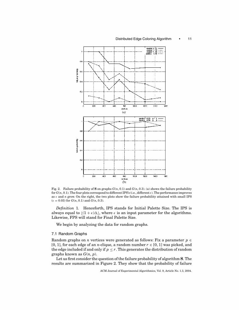
Fig. 2. Failure probability of S on graphs G(n, 0.1) and G(n, 0.3). (a) shows the failure probabilityfor G(n, 0.1). The four plots correspond to different IPS’s (i.e., different ε). The performance improvesas ε and n grow. On the right, the two plots show the failure probability attained with small IPS(ε = 0.03) for G(n, 0.1) and G(n, 0.3).

Definition 1. Henceforth, IPS stands for Initial Palette Size. The IPS isalways equal to �(1 + ε)��, where ε is an input parameter for the algorithms.Likewise, FPS will stand for Final Palette Size.

We begin by analyzing the data for random graphs.

7.1 Random Graphs

Random graphs on n vertices were generated as follows: Fix a parameter p ∈[0, 1], for each edge of an n-clique, a random number r ∈ [0, 1] was picked, andthe edge included if and only if p ≤ r. This generates the distribution of randomgraphs known as G(n, p).

Let us first consider the question of the failure probability of algorithm S. Theresults are summarized in Figure 2. They show that the probability of failure



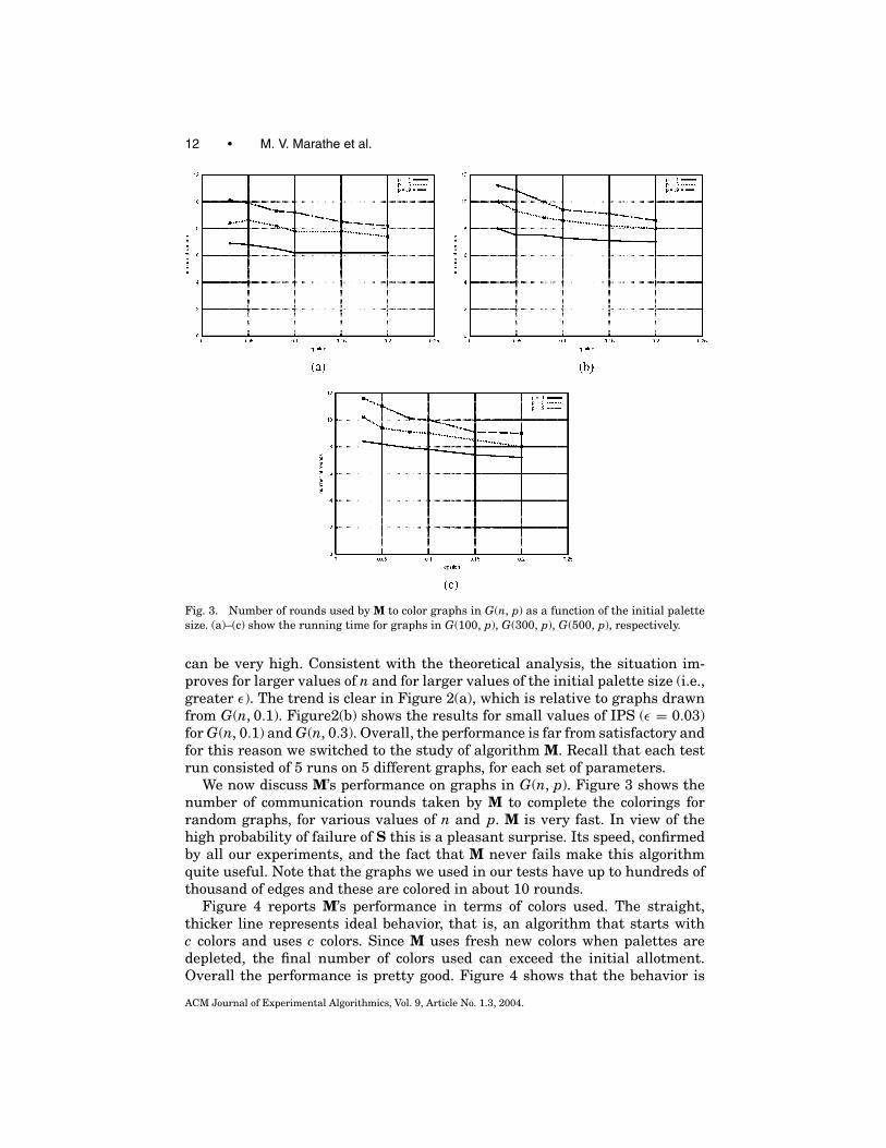
Fig. 3. Number of rounds used by M to color graphs in G(n, p) as a function of the initial palettesize. (a)–(c) show the running time for graphs in G(100, p), G(300, p), G(500, p), respectively.

can be very high. Consistent with the theoretical analysis, the situation im-proves for larger values of n and for larger values of the initial palette size (i.e.,greater ε). The trend is clear in Figure 2(a), which is relative to graphs drawnfrom G(n, 0.1). Figure2(b) shows the results for small values of IPS (ε = 0.03)for G(n, 0.1) and G(n, 0.3). Overall, the performance is far from satisfactory andfor this reason we switched to the study of algorithm M. Recall that each testrun consisted of 5 runs on 5 different graphs, for each set of parameters.

We now discuss M’s performance on graphs in G(n, p). Figure 3 shows thenumber of communication rounds taken by M to complete the colorings forrandom graphs, for various values of n and p. M is very fast. In view of thehigh probability of failure of S this is a pleasant surprise. Its speed, confirmedby all our experiments, and the fact that M never fails make this algorithmquite useful. Note that the graphs we used in our tests have up to hundreds ofthousand of edges and these are colored in about 10 rounds.

Figure 4 reports M’s performance in terms of colors used. The straight,thicker line represents ideal behavior, that is, an algorithm that starts withc colors and uses c colors. Since M uses fresh new colors when palettes aredepleted, the final number of colors used can exceed the initial allotment.Overall the performance is pretty good. Figure 4 shows that the behavior is



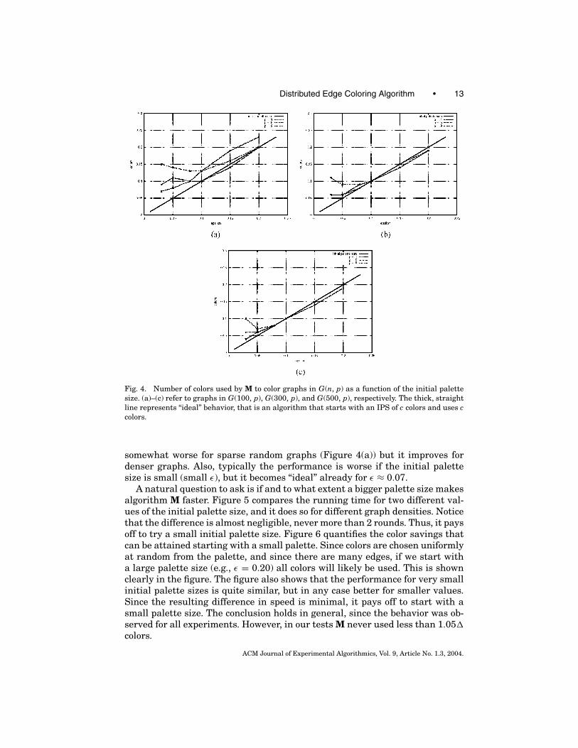
Fig. 4. Number of colors used by M to color graphs in G(n, p) as a function of the initial palettesize. (a)–(c) refer to graphs in G(100, p), G(300, p), and G(500, p), respectively. The thick, straightline represents “ideal” behavior, that is an algorithm that starts with an IPS of c colors and uses ccolors.

somewhat worse for sparse random graphs (Figure 4(a)) but it improves fordenser graphs. Also, typically the performance is worse if the initial palettesize is small (small ε), but it becomes “ideal” already for ε ≈ 0.07.

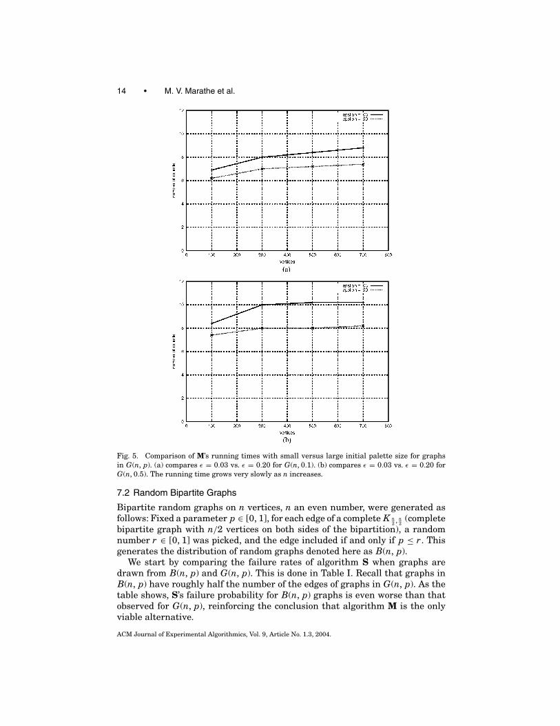
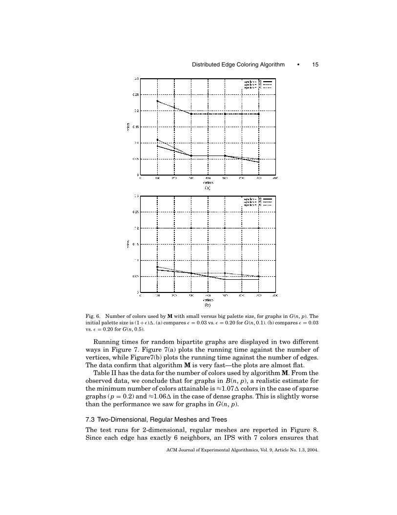
A natural question to ask is if and to what extent a bigger palette size makesalgorithm M faster. Figure 5 compares the running time for two different val-ues of the initial palette size, and it does so for different graph densities. Noticethat the difference is almost negligible, never more than 2 rounds. Thus, it paysoff to try a small initial palette size. Figure 6 quantifies the color savings thatcan be attained starting with a small palette. Since colors are chosen uniformlyat random from the palette, and since there are many edges, if we start witha large palette size (e.g., ε = 0.20) all colors will likely be used. This is shownclearly in the figure. The figure also shows that the performance for very smallinitial palette sizes is quite similar, but in any case better for smaller values.Since the resulting difference in speed is minimal, it pays off to start with asmall palette size. The conclusion holds in general, since the behavior was ob-served for all experiments. However, in our tests M never used less than 1.05�

colors.



Fig. 5. Comparison of M’s running times with small versus large initial palette size for graphsin G(n, p). (a) compares ε = 0.03 vs. ε = 0.20 for G(n, 0.1). (b) compares ε = 0.03 vs. ε = 0.20 forG(n, 0.5). The running time grows very slowly as n increases.

7.2 Random Bipartite Graphs

Bipartite random graphs on n vertices, n an even number, were generated asfollows: Fixed a parameter p ∈ [0, 1], for each edge of a complete K n

2 , n2

(completebipartite graph with n/2 vertices on both sides of the bipartition), a randomnumber r ∈ [0, 1] was picked, and the edge included if and only if p ≤ r. Thisgenerates the distribution of random graphs denoted here as B(n, p).

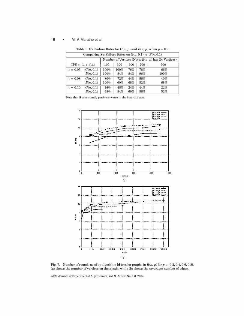
We start by comparing the failure rates of algorithm S when graphs aredrawn from B(n, p) and G(n, p). This is done in Table I. Recall that graphs inB(n, p) have roughly half the number of the edges of graphs in G(n, p). As thetable shows, S’s failure probability for B(n, p) graphs is even worse than thatobserved for G(n, p), reinforcing the conclusion that algorithm M is the onlyviable alternative.



Fig. 6. Number of colors used by M with small versus big palette size, for graphs in G(n, p). Theinitial palette size is (1+ ε)�. (a) compares ε = 0.03 vs. ε = 0.20 for G(n, 0.1). (b) compares ε = 0.03vs. ε = 0.20 for G(n, 0.5).

Running times for random bipartite graphs are displayed in two differentways in Figure 7. Figure 7(a) plots the running time against the number ofvertices, while Figure7(b) plots the running time against the number of edges.The data confirm that algorithm M is very fast—the plots are almost flat.

Table II has the data for the number of colors used by algorithm M. From theobserved data, we conclude that for graphs in B(n, p), a realistic estimate forthe minimum number of colors attainable is ≈1.07� colors in the case of sparsegraphs (p = 0.2) and ≈1.06� in the case of dense graphs. This is slightly worsethan the performance we saw for graphs in G(n, p).

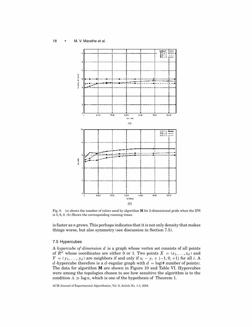
7.3 Two-Dimensional, Regular Meshes and Trees

The test runs for 2-dimensional, regular meshes are reported in Figure 8.Since each edge has exactly 6 neighbors, an IPS with 7 colors ensures that



Table I. S’s Failure Rates for G(n, p) and B(n, p) when p = 0.1

Comparing S’s Failure Rates on G(n, 0.1) vs. B(n, 0.1)

Number of Vertices (Note: B(n, p) has 2n Vertices)

IPS = �(1 + ε)�� 100 300 500 700 900

ε = 0.05 G(n, 0.1) 100% 100% 76% 76% 66%B(n, 0.1) 100% 84% 84% 96% 100%

ε = 0.08 G(n, 0.1) 80% 72% 44% 56% 40%B(n, 0.1) 100% 60% 68% 52% 68%

ε = 0.10 G(n, 0.1) 76% 48% 24% 44% 22%B(n, 0.1) 68% 84% 60% 56% 52%

Note that S consistently performs worse in the bipartite case.

Fig. 7. Number of rounds used by algorithm M to color graphs in B(n, p) for p ∈ {0.2, 0.4, 0.6, 0.8}.(a) shows the number of vertices on the x-axis, while (b) shows the (average) number of edges.



Table II. Number of Colors used by Algorithm M to Color Graphs in B(n, p)

Number of Colors Used by M for Graphs In B(n,p)

Graph Parameters: IPS = �(1 + ε)��Vertices Edges P � ε = 0.03 ε = 0.05 ε = 0.08 ε = 0.10 ε = 0.15 ε = 0.20100 505 0.2 18 0.07 0.07 0.07 0.11 0.12 0.17

1003 0.4 28 0.14 0.11 0.12 0.11 0.19 0.211503 0.6 37 0.14 0.16 0.14 0.14 0.16 0.202000 0.8 47 0.14 0.13 0.12 0.13 0.16 0.20

300 4499 0.2 43 0.08 0.10 0.10 0.12 0.15 0.199001 0.4 77 0.07 0.08 0.09 0.10 0.15 0.20

13,449 0.6 106 0.07 0.08 0.09 0.10 0.14 0.1917,981 0.8 132 0.16 0.11 0.10 0.11 0.15 0.20

500 12,526 0.2 70 0.05 0.07 0.08 0.10 0.15 0.2024,981 0.4 122 0.06 0.07 0.09 0.10 0.15 0.2037,466 0.6 172 0.06 0.06 0.08 0.10 0.15 0.2050,031 0.8 218 0.12 0.08 0.09 0.10 0.14 0.20

700 24,506 0.2 93 0.05 0.07 0.09 0.11 0.15 0.2049,072 0.4 170 0.04 0.06 0.08 0.10 0.15 0.2073,510 0.6 239 0.05 0.06 0.08 0.10 0.15 0.2097,969 0.8 304 0.07 0.06 0.08 0.10 0.15 0.20

900 40,401 0.2 119 0.05 0.06 0.08 0.10 0.15 0.2081,088 0.4 213 0.05 0.06 0.08 0.10 0.15 0.20

121,460 0.6 300 0.06 0.06 0.08 0.10 0.15 0.20162,088 0.8 386 0.07 0.06 0.08 0.10 0.15 0.20

The table shows the percentage of extra colors used. The algorithm starts with IPS = �(1 + ε)�� colors and endsup using with FPS = (1 + δ)�. The table reports the value of δ, rounded to second decimal place.

no palette will ever be depleted. The data show that sometimes the algorithmuses as few as 6 colors but this happens rarely. One might wonder whetherallowing a larger IPS might significantly increase the algorithm’s speed.Figure 8 shows that the answer is “no” and confirms that algorithm M is veryfast.

We tested algorithms S and M on d -regular trees of height �. These are rootedtrees in which the root has height 0 and degree d and every other internal nodehas degree d + 1. Therefore, � = d + 1, n = (d �+1 − 1)/(d − 1), and m = n − 1.In all tests � = 5, while 1 ≤ � ≤ 8. Recall that in trees there is no interactionamong the (implicit) vertex palettes and therefore the process most resemblesthe idealized situation described in Section 5. Since � = 5, nine colors arealways sufficient to color any 4-regular tree. The data show that, as usual,there is no real speed up by using a larger IPS and that as few as seven colorsare sometimes enough for up to a few hundred edges.

7.4 Cliques

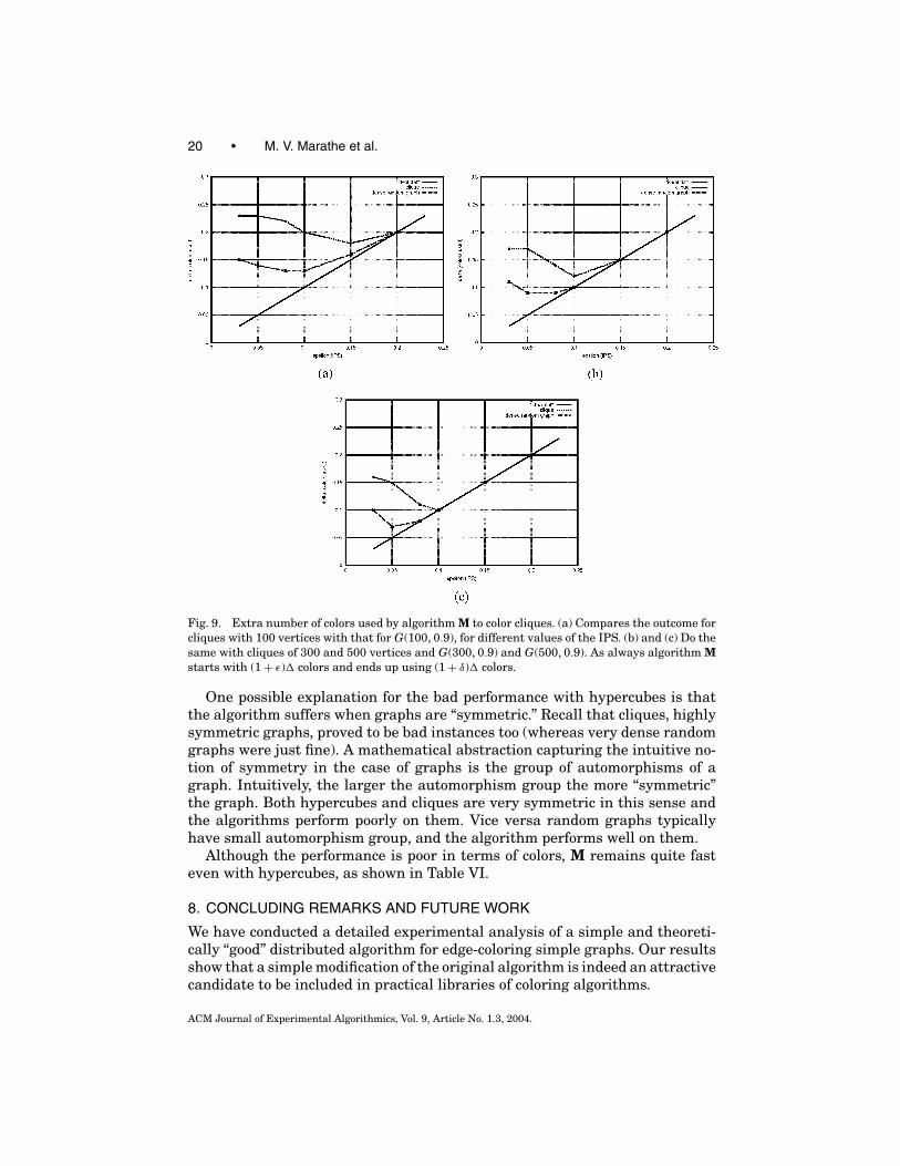
The data for algorithm M are shown in Tables III–V and Figure 9. While thealgorithm remains quite fast (Table III), the performance in terms of colorsdeteriorates when compared to other graphs.

Table III compares the outcome for cliques with that of random graphs ofvery high density (p = 0.9). The performance for dense random graphs is clearlybetter than that for cliques. Not only are the figures better, but the improvement



Fig. 8. (a) shows the number of colors used by algorithm M for 2-dimensional grids when the IPSis 5, 6, 8. (b) Shows the corresponding running times.

is faster as n grows. This perhaps indicates that it is not only density that makesthings worse, but also symmetry (see discussion in Section 7.5).

7.5 Hypercubes

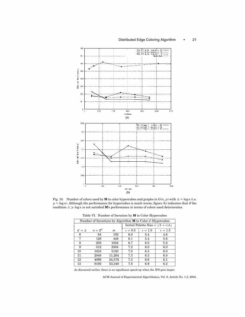
A hypercube of dimension d is a graph whose vertex set consists of all pointsof Rd whose coordinates are either 0 or 1. Two points X = (x1, . . . , xd ) andY = ( y1, . . . , yd ) are neighbors if and only if xi − yi ∈ {−1, 0, +1} for all i. Ad -hypercube therefore is a d -regular graph with d = log(# number of points).The data for algorithm M are shown in Figure 10 and Table VI. Hypercubeswere among the topologies chosen to see how sensitive the algorithm is to thecondition � � log n, which is one of the hypothesis of Theorem 1.



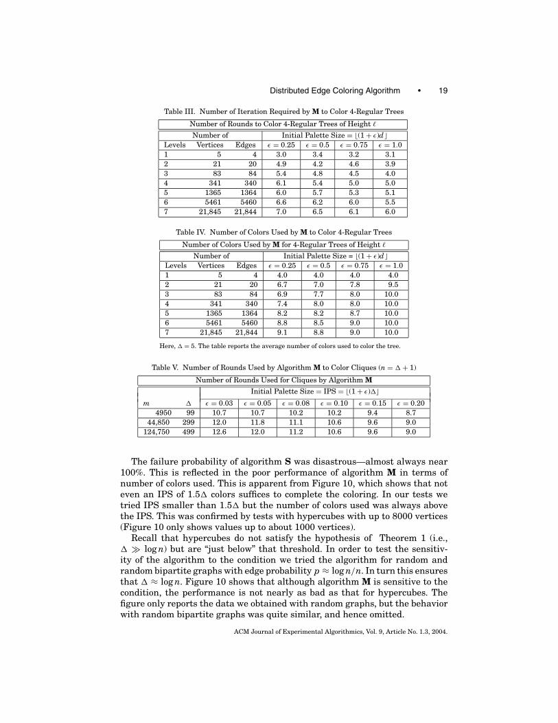
Table III. Number of Iteration Required by M to Color 4-Regular Trees

Number of Rounds to Color 4-Regular Trees of Height �

Number of Initial Palette Size = �(1 + ε)d�Levels Vertices Edges ε = 0.25 ε = 0.5 ε = 0.75 ε = 1.01 5 4 3.0 3.4 3.2 3.12 21 20 4.9 4.2 4.6 3.93 83 84 5.4 4.8 4.5 4.04 341 340 6.1 5.4 5.0 5.05 1365 1364 6.0 5.7 5.3 5.16 5461 5460 6.6 6.2 6.0 5.57 21,845 21,844 7.0 6.5 6.1 6.0

Table IV. Number of Colors Used by M to Color 4-Regular Trees

Number of Colors Used by M for 4-Regular Trees of Height �

Number of Initial Palette Size = �(1 + ε)d�Levels Vertices Edges ε = 0.25 ε = 0.5 ε = 0.75 ε = 1.01 5 4 4.0 4.0 4.0 4.02 21 20 6.7 7.0 7.8 9.53 83 84 6.9 7.7 8.0 10.04 341 340 7.4 8.0 8.0 10.05 1365 1364 8.2 8.2 8.7 10.06 5461 5460 8.8 8.5 9.0 10.07 21,845 21,844 9.1 8.8 9.0 10.0

Here, � = 5. The table reports the average number of colors used to color the tree.

Table V. Number of Rounds Used by Algorithm M to Color Cliques (n = � + 1)

Number of Rounds Used for Cliques by Algorithm M

Initial Palette Size = IPS = �(1 + ε)��m � ε = 0.03 ε = 0.05 ε = 0.08 ε = 0.10 ε = 0.15 ε = 0.20

4950 99 10.7 10.7 10.2 10.2 9.4 8.744,850 299 12.0 11.8 11.1 10.6 9.6 9.0

124,750 499 12.6 12.0 11.2 10.6 9.6 9.0

The failure probability of algorithm S was disastrous—almost always near100%. This is reflected in the poor performance of algorithm M in terms ofnumber of colors used. This is apparent from Figure 10, which shows that noteven an IPS of 1.5� colors suffices to complete the coloring. In our tests wetried IPS smaller than 1.5� but the number of colors used was always abovethe IPS. This was confirmed by tests with hypercubes with up to 8000 vertices(Figure 10 only shows values up to about 1000 vertices).

Recall that hypercubes do not satisfy the hypothesis of Theorem 1 (i.e.,� � log n) but are “just below” that threshold. In order to test the sensitiv-ity of the algorithm to the condition we tried the algorithm for random andrandom bipartite graphs with edge probability p ≈ log n/n. In turn this ensuresthat � ≈ log n. Figure 10 shows that although algorithm M is sensitive to thecondition, the performance is not nearly as bad as that for hypercubes. Thefigure only reports the data we obtained with random graphs, but the behaviorwith random bipartite graphs was quite similar, and hence omitted.



Fig. 9. Extra number of colors used by algorithm M to color cliques. (a) Compares the outcome forcliques with 100 vertices with that for G(100, 0.9), for different values of the IPS. (b) and (c) Do thesame with cliques of 300 and 500 vertices and G(300, 0.9) and G(500, 0.9). As always algorithm Mstarts with (1 + ε)� colors and ends up using (1 + δ)� colors.

One possible explanation for the bad performance with hypercubes is thatthe algorithm suffers when graphs are “symmetric.” Recall that cliques, highlysymmetric graphs, proved to be bad instances too (whereas very dense randomgraphs were just fine). A mathematical abstraction capturing the intuitive no-tion of symmetry in the case of graphs is the group of automorphisms of agraph. Intuitively, the larger the automorphism group the more “symmetric”the graph. Both hypercubes and cliques are very symmetric in this sense andthe algorithms perform poorly on them. Vice versa random graphs typicallyhave small automorphism group, and the algorithm performs well on them.

Although the performance is poor in terms of colors, M remains quite fasteven with hypercubes, as shown in Table VI.

8. CONCLUDING REMARKS AND FUTURE WORK

We have conducted a detailed experimental analysis of a simple and theoreti-cally “good” distributed algorithm for edge-coloring simple graphs. Our resultsshow that a simple modification of the original algorithm is indeed an attractivecandidate to be included in practical libraries of coloring algorithms.



Fig. 10. Number of colors used by M to color hypercubes and graphs in G(n, p) with � ≈ log n (i.e.p ≈ log n). Although the performance for hypercubes is much worse, figure (b) indicates that if thecondition � � log n is not satisfied M’s performance in terms of colors used deteriorates.

Table VI. Number of Iteration by M to Color Hypercubes

Number of Iterations by Algorithm M to Color d -HypercubesInitial Palette Size = �(1 + ε)��

d = � n = 2d m ε = 0.5 ε = 1.0 ε = 1.56 64 192 6.0 5.4 4.67 128 448 6.1 5.4 5.68 256 1024 6.7 6.0 5.29 512 2304 7.2 6.0 6.0

10 1024 5120 7.0 6.3 6.011 2048 11,264 7.3 6.3 6.012 4096 24,576 7.3 6.6 6.113 8192 53,248 7.8 6.9 6.2

As discussed earlier, there is no significant speed-up when the IPS gets larger.



ACKNOWLEDGMENTS

We thank Olaf Lubeck, Robert Ferrell and Joseph Kanapka for introducing usto PGSLib and working with us closely during the initial parts of the project.We thank Dr. Ravi Jain (Telecordia) for making available a copy of his papers.Finally, we thank Prof. T. Luzack, Prof. S.S. Ravi Dr. Vance Faber and Prof.Aravind Srinivasan for several discussions on related topics.

REFERENCES

DUBHASHI, D., GRABLE, D., AND PANCONESI, A. 1998. Nearly-optimal, distributed edge-coloring viathe nibble method. TCS 203, 4, 225–251. A special issue for the best papers of the 3rd EuropeanSymposium on Algorithms (ESA 95).

DURAND, D., JAIN, R., AND TSEYTLIN, D. 1994. Distributed Scheduling Algorithms to Improve thePerformance of Parallel Data Transfers. In ACM SIGARCH Computer Architecture News. ACMPress, 35–40. Special issue on Input/Output in Parallel Computer Systems.

DURAND, D., JAIN, R., AND TSEYTLIN, D. 1998. Applying randomized edge-coloring algorithms todistributed communications: An experimental study. TCS 203, 4, 225–251. A special issue forthe best papers of the 3rd European Symposium on Algorithms (ESA 95).

FERRELL, R., KOTHE, D., AND TURNER, J. 1997. PGSLib: A library for portable, parallel, unstructuredmesh simulations. In Presented at the 8th SIAM Conference on Parallel Processing for ScientificComputing.

FINOCCHI, I., PANCONESI, A., AND SILVESTRI, R. 2002. An experimental study of simple, distributedvertex colouring algorithms. In Proceedings of the Thirteenth ACM-SIAM Symposium on DiscreteAlgorithms (SODA 02). ACM Press, 245–269. To appear in Algorithmica.

GABOW, H. AND KARIV, O. 1982. Algorithms for edge-coloring bipartite graphs and multigraphs.SIAM J. Comput. 1, 11, 117–129.

GRABLE, D. AND PANCONESI, A. 1997. Nearly optimal distributed edge-coloring in o(log log n)rounds. RSA 10, 3 (May), 385–405. Also In Proceedings of the 9th ACM-SIAM Symposium onDiscrete Algorithms (SODA), 1997, pp. 278–285.

HOCHBAUM, D., Eds. 1997. Approximation Algorithms for NP-Hard Problems. PWS PublishingCompany, Boston, MA.

HOYLER, I. 1980. The NP-completeness of edge colorings. SIAM J. Comput. 10, 718–720.JAIN, R., SOMALWAR, K., WERTH, J., AND BROWNE, J. 1992a. Scheduling parallel I/O operations in

multiple bus systems. J. Parallel Distrib. Comput. 16, 4, 352–362.JAIN, R., WERTH, J., BROWNE, J., AND SASAKI, G. 1992b. A graph-theoretic model for the scheduling

problem and its application to simultaneous resource scheduling. In Computer Science and Op-erations Research: New Developments in Their Interfaces. O. Balci, R. Shander, and S. Zerrick,Eds. Penguin Press.

JAIN, R. AND WERTH, J. 1995. Analysis of approximate algorithms for edge-coloring bipartitegraphs. IPL 54, 3, 163–168.

KOTHE, D., FERRELL, R., TURNER, J., AND MOSSO, S. 1997. A high resolution finite volume methodfor efficient parallel simulation of casting processes on unstructured meshes. In Presented at the8th SIAM Conference on Parallel Processing for Scientific Comput. LANL Report LA-UR-97-30,14–17.

PANCONESI, A. AND SRINIVASAN, A. 1992. Fast randomized algorithms for distributed edge coloring.SIAM J. Comput. 26, 2, 350–368. Also in Proceedings of the ACM Symposium on Principles ofDistributed Computing (PODC) 1992.


Documents

An Experimental Study of a Simple, Distributed Edge-Coloring Algorithm