Embed Size (px)
Citation preview
VOL. 6, NO. 9, SEPTEMBER 2011 ISSN 1819-6608
ARPN Journal of Engineering and Applied Sciences
©2006-2011 Asian Research Publishing Network (ARPN). All rights reserved.
www.arpnjournals.com
78
AN EXPERT MODEL FOR THE SHELL AND TUBE HEAT EXCHANGERS ANALYSIS BY ARTIFICIAL NEURAL NETWORKS
A.R. Moghadassi1, S.M. Hosseini1, F. Parvizian1, F. Mohamadiyon1, A. Behzadi Moghadam1 and A. Sanaeirad2
1Department of Chemical Engineering, Faculty of Engineering, Arak University, Arak, Iran 2Department of Civil Engineering, Faculty of Engineering, Arak University, Arak, Iran
E-Mail: [email protected] ABSTRACT
Due to the importance of heat exchangers in chemical and petrochical industries, heat exchangers analysis and heat translate calculations are preceded. The conventional and prevalent methods (such as KERN method and etc) are presented heat translate calculation for the analysis and selection of shell and tube heat exchanger based on the obtained pressure drop and fouling factor after consecutive calculation. Also there are many properties and parameters in prevalent methods. The current work proposed a new method based on the artificial neural network (ANN) for the analysis of Shell and Tube Heat Exchangers. Special parameters for heat exchangers analysis were obtained by neural network and the required experimental data were collected form Kern’s book, TEMA and Perry’s handbook. The work used back- propagation learning algorithm incorporating levenberg- marquardt training method. The accuracy and trend stability of the trained networks were verified according to their ability to predict unseen data. MSE error evaluation was used and the error limitation is 10-3-10-6. Parameters can be obtained without using charts, different tables and complicated equations. During this research, twenty two networks were utilized for all different properties. The results demonstrated the ANN’s capability to predict the analysis. Keywords: model, shell and tube heat exchanger, analysis, KERN method, artificial neural network. Nomenclature
A Heat-transfer surface ft2 B Baffle spacing in C,c Specific heat of fluid Btu/(lb)(oF) De
Equivalent diameter for heat transfer and pressure drop ft
Fc Caloric Fraction FT Temperature difference factor f Friction factor ID Inside diameter in jH Factor for heat transfer Kc Caloric constant k Thermal conductivity Btu/(hr)(ft2)(oF/ft) L Tube length ft LMTD Log mean temperature difference oF Nt Number of tubes n Number of tube passes PT Tube pitch in Ps ∆ Pt,∆
Tube side and return pressure drop, respectively psi
Q Heat flow Btu/hr R Temperature group, (T1-T2)/(t2-t1) Re Reynolds number for heat transfer and pressure
drop S Temperature group,(t2-t1)/(T1-t1) s Specific gravity tw Tube wall temperature oF φ The viscosity ratio (µ/µw)0.14 µ Viscosity lb/(ft)(hr) µw Viscosity at wall temperature lb/(ft)(hr)
1. INTRODUCTION Heat exchangers may be classified according to
their flow arrangement. Counter current heat exchangers are most efficient because they allow the highest log mean temperature difference between the hot and cold streams. In a cross-flow heat exchanger, the fluids travel roughly perpendicular to one another through the exchanger. For efficiency, heat exchangers are designed to maximize the surface area of the wall between the two fluids, while minimizing resistance to fluid flow through the exchanger. The exchanger's performance can also be affected by the addition of fins or corrugations in one or both directions, which increase surface area and may channel fluid flow or induce turbulence. The driving temperature across the heat transfer surface varies with position, but an appropriate mean temperature can be defined. In most simple systems this is the log mean temperature difference (LMTD). Sometimes direct knowledge of the LMTD is not available and the NTU method is used.
Fouling occurs when a fluid goes through the heat exchanger, and the impurities in the fluid precipitate onto the surface of the tubes. Precipitation of these impurities can be caused by: Frequent use of the heat exchanger, Not cleaning the heat exchanger regularly, Reducing the velocity of the fluids moving through the heat exchanger and Over-sizing of the heat exchanger. Effects of fouling are more abundant in the cold tubes of the heat exchanger than in the hot tubes. This is because impurities are less likely to be dissolved in a cold fluid. This is because, for most substances, solubility increases as temperature increases. A notable exception is hard water where the opposite is true. Fouling reduces the cross sectional area for heat to be transferred and causes an increase in the resistance to heat transfer across the heat
VOL. 6, NO. 9, SEPTEMBER 2011 ISSN 1819-6608
ARPN Journal of Engineering and Applied Sciences
©2006-2011 Asian Research Publishing Network (ARPN). All rights reserved.
www.arpnjournals.com
79
exchanger. This is because the thermal conductivity of the fouling layer is low. This reduces the overall heat transfer coefficient and efficiency of the heat exchanger. This in turn, can lead to an increase in pumping and maintenance costs. The conventional approach to fouling control combines the “blind” application of biocides and anti-scale chemicals with periodic lab testing. This often results in the excessive use of chemicals with the inherent side effects of accelerating system corrosion and increasing toxic waste - not to mention the incremental cost of unnecessary treatments. There are however solutions for continuous fouling monitoring In liquid environments, such as the Neosens FS sensor, measuring both fouling thickness and temperature, allowing to optimize the use of chemicals and control the efficiency of cleanings. 2. MAINTENANCE
Plate heat exchangers need to be dissembled and cleaned periodically. Tubular heat exchangers can be cleaned by such methods as acid cleaning, sandblasting, high-pressure water jet, bullet cleaning, or drill rods. In large-scale cooling water systems for heat exchangers, water treatment such as purification, addition of chemicals, and testing, is used to minimize fouling of the heat exchange equipment. Other water treatment is also used in steam systems for power plants, etc. to minimize fouling and corrosion of the heat exchange and other equipment. A variety of companies have started using water borne oscillations technology to prevent biofouling. Without the use of chemicals, this type of technology has helped in providing a low-pressure drop in heat exchangers [1, 2].
3. THE ALGORITHM CALCULATION OF A SHELL AND TUBE EXCHANGER
Process conditions required:
Hot fluid: T1, T2, W, C, s, µ, k, Rd, ∆P
Cold fluid: t1, t2, w, c, s, µ, k, Rd, ∆P
For the exchanger the following data must be known: Shell side: ID, Baffle space, passes
Tube side: Number and length, OD, BWG, and pitch, Passes
(1) From T1, T2, t1, t2 check the heat balance, Q, using c at Tmean and tmean.
Q=WC (T1-T2) = wc (t2-t1) (1)
T,t(F)، W, w (lb/hr)، C, c (Btu/lb. F) ،) Btu/hr(Q
(2) Ture temperature difference ∆t: (Assuming conuter flow)
LMED= [(T1-t2)-(T2-t1)]/ [ln (T1-t2)/ (T2-t1)] (2)
R=(T1-T2)/(t2-t1), S=(t2-t1)/(T1-t1) => FT∆
t=LMTD×FT (3)
(3) Caloric temperature Tc , tc :
Tc=T2+Fc(T1-T2) (4)
tc=t1+Fc(t2-t1) (5)
The coleric fraction Fc can be obtained from experimental results [3 by computing Kc from Uh and Uc and ∆tc/∆th for the process conditions. If neither of the liquids is very viscous at the cold terminal, say not more than 1.0 centipoies, if the temperature ranges do not exceed 50 to 100oF, and if the temperature difference is less than 50oF, the arithmetic means of T1and T2 and t1nad t2 may be used in place of Tc and tc for evaluating the physical properties.
Cold fluid: tube side (4) Flow area, at.
Flow area per tube at´ (in2) [3].
Nt. at´/144n, (ft2) =at (6)
(5) Mass vel,Gt.
GT=w/at, (Lb/hr.ft2) (7)
(6) Obtain D from Table (10), ft. Obtain µ at tc,lb/(ft)(hr)=cp×2.24 Res=De. Gt/µ (8)
(7) Obtain jH [3] (8) At tc obtain c,Btu/(lb)(oF) and k, Btu/(hr)(ft2)(oF/ft). Compute (cµ/k) 1/3
(9) hi = jH.(k/D).(cµ/k)1/3.Φt (9)
(10) hio/Φt=hi/ Φt×ID/OD (10)
(11) Obtain tw from (10´). Obtain µw and Φt= (µ/µw) 0.14.
(12) Corrected coefficient, hio= (hio/Φt) ×Φt, (Btu/hr.ft2.F) Hot fluid: shell side
(4´) flow area as.
as=ID.C.B/144.PT, (ft2) (11)
(5´) Mass vel, Gs.
(Lb/hr.ft2) Gs=w/as,
(6´) compute De=4×free area/wetted perimeter, (ft) (12)
de = 4×(PT-πdo2/4)/πdo, (in) (13)
Obtain µ at Tc, lb/ (ft) (hr) =cp×2.24 Res=De. Gs/µ
(7´) Obtain jH [3]
(8´) At Tc obtain C, Btu/ (lb) (oF) and k, Btu/ (hr) (ft2) (oF/ft). (8´) Compute (cµ/k) 1/3
(9´) ho=jH. (k/De).(c.µ/k)1/3.Φs
(10´) Tube wall tem, tw.
tw = tc+[(ho/Φs)/((hio/Φt)+(ho/Φs))]×(Tc-tc) (14)
(11´) Obtain µw and Φs= (µ/µw) 0.14.
(12´) Corrected coefficient, ho= (hio/Φs) ×Φs
VOL. 6, NO. 9, SEPTEMBER 2011 ISSN 1819-6608
ARPN Journal of Engineering and Applied Sciences
©2006-2011 Asian Research Publishing Network (ARPN). All rights reserved.
www.arpnjournals.com
80
(13) Clean overall coefficient Uc:
Uc= (hio. ho)/ (hio+ho) (15)
(14) Design overall coefficient UD: obtain external surface/lin ft a˝ from Table-10. Heat transfer surface, A= a˝LNt, (ft2)
UD=Q/A˝∆t, (Btu/hr.ft2.F) (16)
(15) Dirt factor Rd:
Rd= (Uc-UD)/Uc. UD, (hr.ft2.F/Btu) (17)
If Rd equals or exceeds the required dirt factor, proceed under the pressure drop. Pressure drop
(1) For Ret in (6) obtain f, ft2/in2.
(2) ∆Pt= (f.Gt2.Ln)/ (5.22×1010.D.s.Φt), (psi) (18)
(3) ∆Pr = (4.n/s) × (V2/2g), (psi) (19)
PT=∆Pt+∆Pr, (psi) ∆
(1´) For Res in (6´) obtain f, ft2/in2.
(2´) No. of crosses, N+1=12L/B (20)
(3´) ∆Ps= (f.Gs2.Ds. (N+1))/ (5.22×10¹⁰.De.s.Φs) [3], (psi)
4. ARTIFICIAL NEURAL NETWORKS
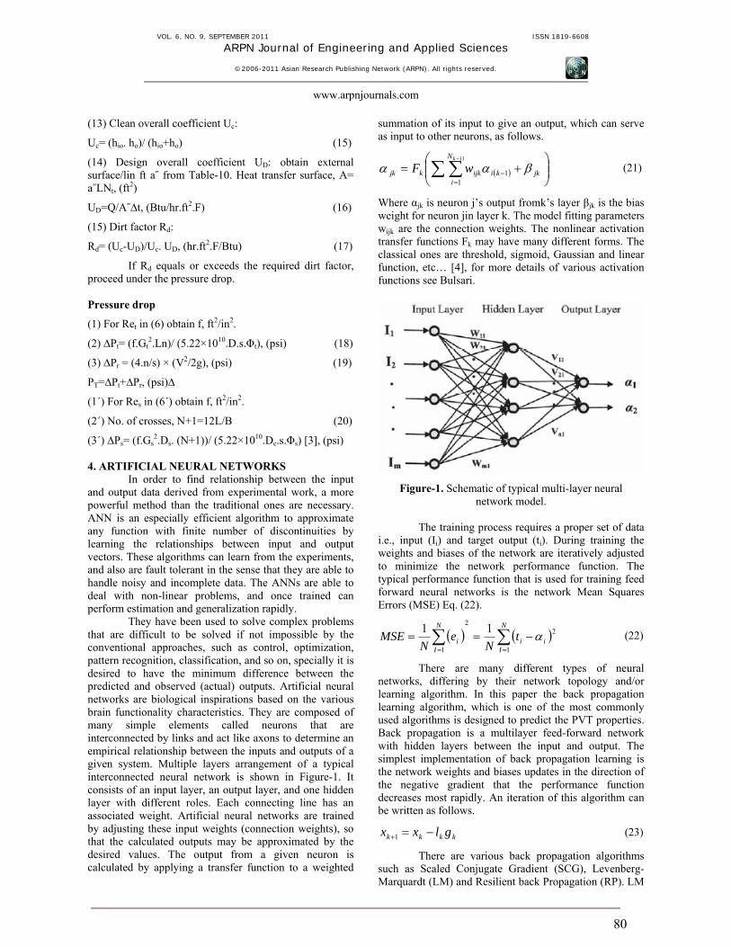
In order to find relationship between the input and output data derived from experimental work, a more powerful method than the traditional ones are necessary. ANN is an especially efficient algorithm to approximate any function with finite number of discontinuities by learning the relationships between input and output vectors. These algorithms can learn from the experiments, and also are fault tolerant in the sense that they are able to handle noisy and incomplete data. The ANNs are able to deal with non-linear problems, and once trained can perform estimation and generalization rapidly.
They have been used to solve complex problems that are difficult to be solved if not impossible by the conventional approaches, such as control, optimization, pattern recognition, classification, and so on, specially it is desired to have the minimum difference between the predicted and observed (actual) outputs. Artificial neural networks are biological inspirations based on the various brain functionality characteristics. They are composed of many simple elements called neurons that are interconnected by links and act like axons to determine an empirical relationship between the inputs and outputs of a given system. Multiple layers arrangement of a typical interconnected neural network is shown in Figure-1. It consists of an input layer, an output layer, and one hidden layer with different roles. Each connecting line has an associated weight. Artificial neural networks are trained by adjusting these input weights (connection weights), so that the calculated outputs may be approximated by the desired values. The output from a given neuron is calculated by applying a transfer function to a weighted
summation of its input to give an output, which can serve as input to other neurons, as follows.
( ) ⎟⎟⎠
⎞⎜⎜⎝
⎛+= ∑ ∑
−
=−
11
11
kN
ijkkiijkkjk wF βαα (21)
Where αjk is neuron j’s output fromk’s layer βjk is the bias weight for neuron jin layer k. The model fitting parameters wijk are the connection weights. The nonlinear activation transfer functions Fk may have many different forms. The classical ones are threshold, sigmoid, Gaussian and linear function, etc… [4], for more details of various activation functions see Bulsari.
Figure-1. Schematic of typical multi-layer neural network model.
The training process requires a proper set of data
i.e., input (Ii) and target output (ti). During training the weights and biases of the network are iteratively adjusted to minimize the network performance function. The typical performance function that is used for training feed forward neural networks is the network Mean Squares Errors (MSE) Eq. (22).
( ) ( )∑∑==
−==N
Iii
N
Ii t
Ne
NMSE
1
22
1
11 α (22)
There are many different types of neural networks, differing by their network topology and/or learning algorithm. In this paper the back propagation learning algorithm, which is one of the most commonly used algorithms is designed to predict the PVT properties. Back propagation is a multilayer feed-forward network with hidden layers between the input and output. The simplest implementation of back propagation learning is the network weights and biases updates in the direction of the negative gradient that the performance function decreases most rapidly. An iteration of this algorithm can be written as follows.
kkkk glxx −=+1 (23)
There are various back propagation algorithms such as Scaled Conjugate Gradient (SCG), Levenberg-Marquardt (LM) and Resilient back Propagation (RP). LM
VOL. 6, NO. 9, SEPTEMBER 2011 ISSN 1819-6608
ARPN Journal of Engineering and Applied Sciences
©2006-2011 Asian Research Publishing Network (ARPN). All rights reserved.
www.arpnjournals.com
81
is the fastest training algorithm for networks of moderate size and it has the memory reduction feature to be used when the training set is large. One of the most important general purpose back propagation training algorithms is SCG.
The neural nets learn to recognize the patterns of the data sets during the training process. Neural nets teach themselves the patterns of the data set letting the analyst to perform more interesting flexible work in a changing environment. Although neural network may take some time to learn a sudden drastic change, but it is excellent to adapt constantly changing information. However the programmed systems are constrained by the designed situation and they are not valid otherwise. Neural networks build informative models whereas the more conventional models fail to do so. Because of handling very complex interactions, the neural networks can easily model data, which are too difficult to model traditionally (inferential statistics or programming logic). Performance of neural networks is at least as good as classical statistical modeling, and even better in most cases. The neural networks built models are more reflective of the data structure and are significantly faster.
Neural networks now operate well with modest computer hardware. Although neural networks are computationally intensive, the routines have been optimized to the point that they can now run in reasonable time on personal computers. They do not require
supercomputers as they did in the early days of neural network research [5, 6]. 5. NEURAL NETWORK MODEL DEVELOPMENT
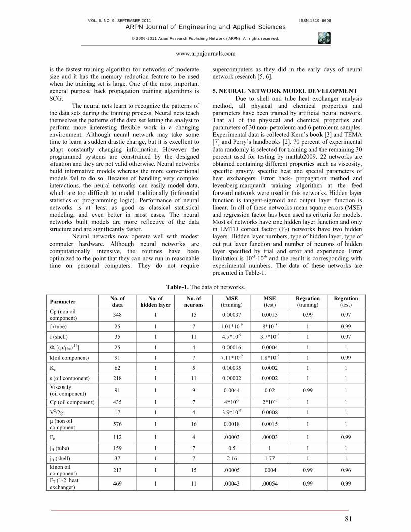
Due to shell and tube heat exchanger analysis method, all physical and chemical properties and parameters have been trained by artificial neural network. That all of the physical and chemical properties and parameters of 30 non- petroleum and 6 petroleum samples. Experimental data is collected Kern’s book [3] and TEMA [7] and Perry’s handbooks [2]. 70 percent of experimental data randomly is selected for training and the remaining 30 percent used for testing by matlab2009. 22 networks are obtained containing different properties such as viscosity, specific gravity, specific heat and special parameters of heat exchangers. Error back- propagation method and levenberg-marquardt training algorithm at the feed forward network were used in this networks. Hidden layer function is tangent-sigmoid and output layer function is linear. In all of these networks mean square errors (MSE) and regression factor has been used as criteria for models. Most of networks have one hidden layer function and only in LMTD correct factor (FT) networks have two hidden layers. Hidden layer numbers, type of hidden layer, type of out put layer function and number of neurons of hidden layer specified by trial and error and experience. Error limitation is 10-3-10-6 and the result is corresponding with experimental numbers. The data of these networks are presented in Table-1.
Table-1. The data of networks.
Parameter No. of data
No. of hidden layer
No. of neurons
MSE (training)
MSE (test)
Regration (training)
Regration (test)
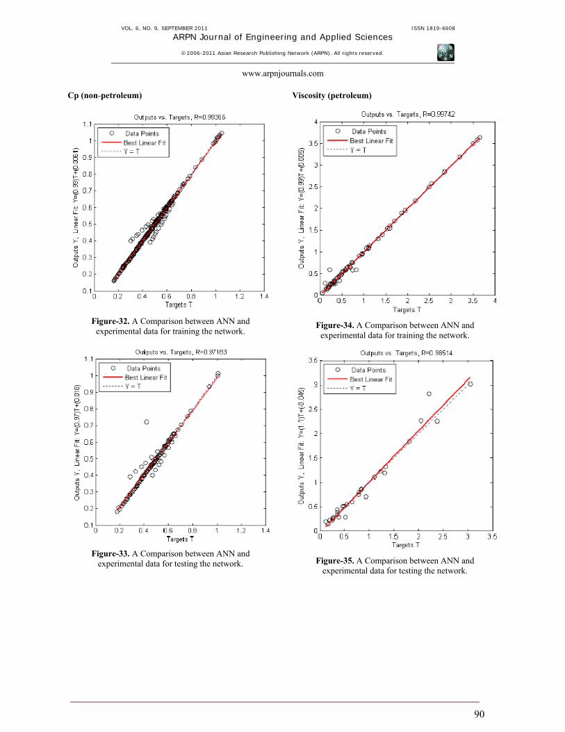
Cp (non oil component) 348 1 15 0.00037 0.0013 0.99 0.97
f (tube) 25 1 7 1.01*10-9 8*10-8 1 0.99
f (shell) 35 1 11 4.7*10-9 3.7*10-6 1 0.97
Фt [(µ/µw).14] 25 1 4 0.00016 0.0004 1 1
k(oil component) 91 1 7 7.11*10-9 1.8*10-6 1 0.99
Kc 62 1 5 0.00035 0.0002 1 1
s (oil component) 218 1 11 0.00002 0.0002 1 1 Viscosity (oil component) 91 1 9 0.0044 0.02 0.99 1
Cp (oil component) 435 1 7 4*10-5 2*10-5 1 1
V2/2g 17 1 4 3.9*10-9 0.0008 1 1 µ (non oil component 576 1 16 0.0018 0.0015 1 1
Fc 112 1 4 .00003 .00003 1 0.99
jH (tube) 159 1 7 0.5 1 1 1
jH (shell) 37 1 7 2.16 1.77 1 1 k(non oil component) 213 1 15 .00005 .0004 0.99 0.96
FT (1-2 heat exchanger) 469 1 11 .00043 .00054 0.99 0.99
VOL. 6, NO. 9, SEPTEMBER 2011 ISSN 1819-6608
ARPN Journal of Engineering and Applied Sciences
©2006-2011 Asian Research Publishing Network (ARPN). All rights reserved.
www.arpnjournals.com
82
FT (2-4 heat exchanger) 480 2 7,9 .0008 .0005 1 0.97
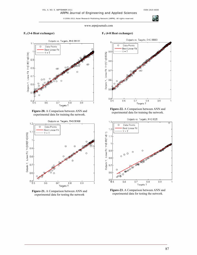
FT (3-6 heat exchanger) 493 2 9,9 .00036 .00063 0.98 0.98
FT (4-8 heat exchanger) 473 2 7,7 .00006 .0032 0.99 0.9
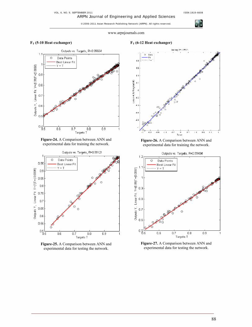
FT (5-10 heat exchanger) 257 2 7,5 .00029 .00012 1 1
FT (6-12 heat exchanger) 290 2 7,5 .00014 .00021 0.99 0.99
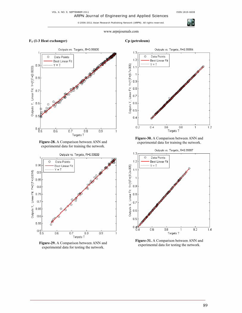
FT (1-3 heat exchanger) 245 1 9 .00008 .00009 1 1
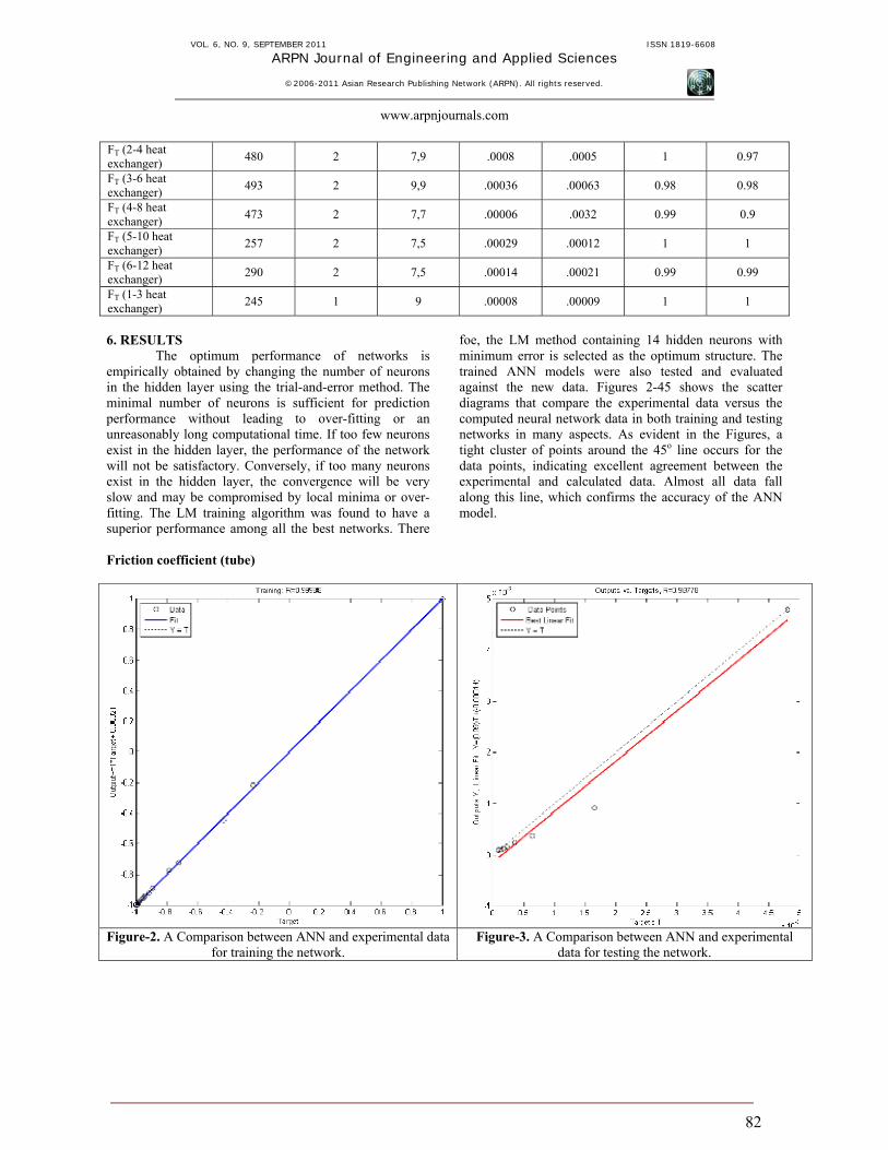
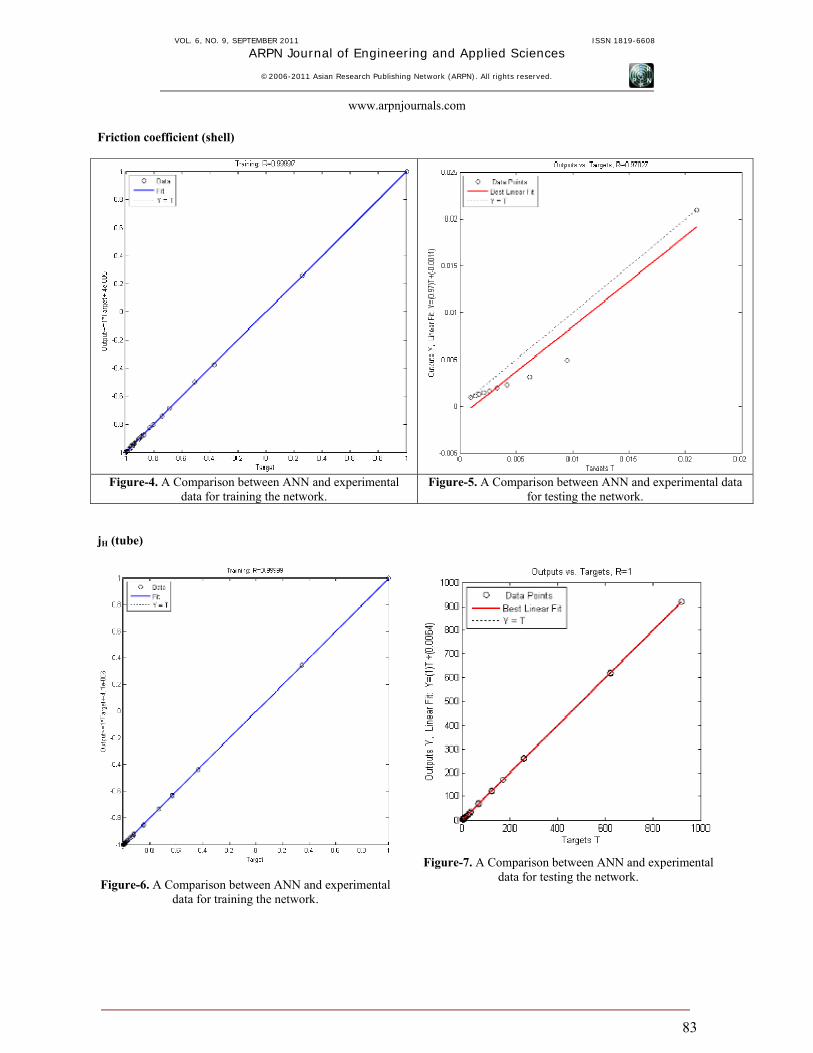
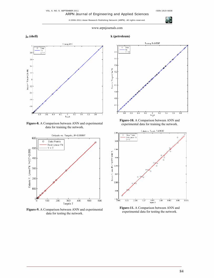
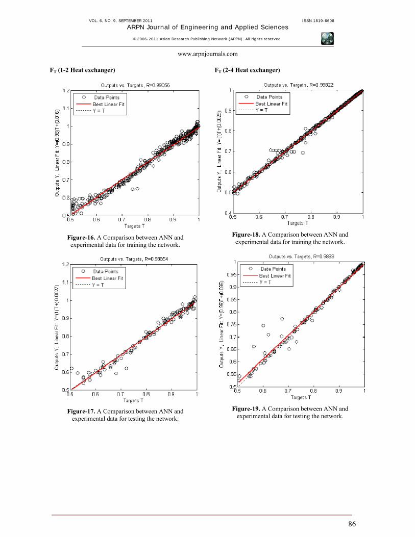
6. RESULTS
The optimum performance of networks is empirically obtained by changing the number of neurons in the hidden layer using the trial-and-error method. The minimal number of neurons is sufficient for prediction performance without leading to over-fitting or an unreasonably long computational time. If too few neurons exist in the hidden layer, the performance of the network will not be satisfactory. Conversely, if too many neurons exist in the hidden layer, the convergence will be very slow and may be compromised by local minima or over-fitting. The LM training algorithm was found to have a superior performance among all the best networks. There
foe, the LM method containing 14 hidden neurons with minimum error is selected as the optimum structure. The trained ANN models were also tested and evaluated against the new data. Figures 2-45 shows the scatter diagrams that compare the experimental data versus the computed neural network data in both training and testing networks in many aspects. As evident in the Figures, a tight cluster of points around the 45o line occurs for the data points, indicating excellent agreement between the experimental and calculated data. Almost all data fall along this line, which confirms the accuracy of the ANN model.
Friction coefficient (tube)
Figure-2. A Comparison between ANN and experimental data
for training the network. Figure-3. A Comparison between ANN and experimental
data for testing the network.
VOL. 6, NO. 9, SEPTEMBER 2011 ISSN 1819-6608
ARPN Journal of Engineering and Applied Sciences
©2006-2011 Asian Research Publishing Network (ARPN). All rights reserved.
www.arpnjournals.com
83
Friction coefficient (shell)
Figure-4. A Comparison between ANN and experimental
data for training the network. Figure-5. A Comparison between ANN and experimental data
for testing the network. jH (tube)
Figure-6. A Comparison between ANN and experimental data for training the network.
Figure-7. A Comparison between ANN and experimental data for testing the network.
VOL. 6, NO. 9, SEPTEMBER 2011 ISSN 1819-6608
ARPN Journal of Engineering and Applied Sciences
©2006-2011 Asian Research Publishing Network (ARPN). All rights reserved.
www.arpnjournals.com
84
jH (shell)
Figure-8. A Comparison between ANN and experimental data for training the network.
Figure-9. A Comparison between ANN and experimental data for testing the network.
k (petroleum)
Figure-10. A Comparison between ANN and experimental data for training the network.
Figure-11. A Comparison between ANN and experimental data for testing the network.

VOL. 6, NO. 9, SEPTEMBER 2011 ISSN 1819-6608
ARPN Journal of Engineering and Applied Sciences
©2006-2011 Asian Research Publishing Network (ARPN). All rights reserved.
www.arpnjournals.com
85
k (non-petroleum)
Figure-12. A Comparison between ANN and experimental data for training the network.
Figure-13. A Comparison between ANN and experimental data for testing the network.
s (petroleum)
Figure-14. A Comparison between ANN and experimental data for training the network.
Figure-15. A Comparison between ANN and experimental data for testing the network.
VOL. 6, NO. 9, SEPTEMBER 2011 ISSN 1819-6608
ARPN Journal of Engineering and Applied Sciences
©2006-2011 Asian Research Publishing Network (ARPN). All rights reserved.
www.arpnjournals.com
86
FT (1-2 Heat exchanger)
Figure-16. A Comparison between ANN and experimental data for training the network.
Figure-17. A Comparison between ANN and experimental data for testing the network.
FT (2-4 Heat exchanger)
Figure-18. A Comparison between ANN and experimental data for training the network.
Figure-19. A Comparison between ANN and experimental data for testing the network.
VOL. 6, NO. 9, SEPTEMBER 2011 ISSN 1819-6608
ARPN Journal of Engineering and Applied Sciences
©2006-2011 Asian Research Publishing Network (ARPN). All rights reserved.
www.arpnjournals.com
87
FT (3-6 Heat exchanger)
Figure-20. A Comparison between ANN and experimental data for training the network.
Figure-21. A Comparison between ANN and experimental data for testing the network
FT (4-8 Heat exchanger)
Figure-22. A Comparison between ANN and experimental data for training the network.
Figure-23. A Comparison between ANN and experimental data for testing the network.
VOL. 6, NO. 9, SEPTEMBER 2011 ISSN 1819-6608
ARPN Journal of Engineering and Applied Sciences
©2006-2011 Asian Research Publishing Network (ARPN). All rights reserved.
www.arpnjournals.com
88
FT (5-10 Heat exchanger)
Figure-24. A Comparison between ANN and experimental data for training the network.
Figure-25. A Comparison between ANN and experimental data for testing the network.
FT (6-12 Heat exchanger)
Figure-26. A Comparison between ANN and experimental data for training the network.
Figure-27. A Comparison between ANN and experimental data for testing the network.
VOL. 6, NO. 9, SEPTEMBER 2011 ISSN 1819-6608
ARPN Journal of Engineering and Applied Sciences
©2006-2011 Asian Research Publishing Network (ARPN). All rights reserved.
www.arpnjournals.com
89
FT (1-3 Heat exchanger)
Figure-28. A Comparison between ANN and experimental data for training the network.
Figure-29. A Comparison between ANN and experimental data for testing the network.
Cp (petroleum)
Figure-30. A Comparison between ANN and experimental data for training the network.
Figure-31. A Comparison between ANN and experimental data for testing the network.
VOL. 6, NO. 9, SEPTEMBER 2011 ISSN 1819-6608
ARPN Journal of Engineering and Applied Sciences
©2006-2011 Asian Research Publishing Network (ARPN). All rights reserved.
www.arpnjournals.com
90
Cp (non-petroleum)
Figure-32. A Comparison between ANN and experimental data for training the network.
Figure-33. A Comparison between ANN and experimental data for testing the network.
Viscosity (petroleum)
Figure-34. A Comparison between ANN and experimental data for training the network.
Figure-35. A Comparison between ANN and experimental data for testing the network.
VOL. 6, NO. 9, SEPTEMBER 2011 ISSN 1819-6608
ARPN Journal of Engineering and Applied Sciences
©2006-2011 Asian Research Publishing Network (ARPN). All rights reserved.
www.arpnjournals.com
91
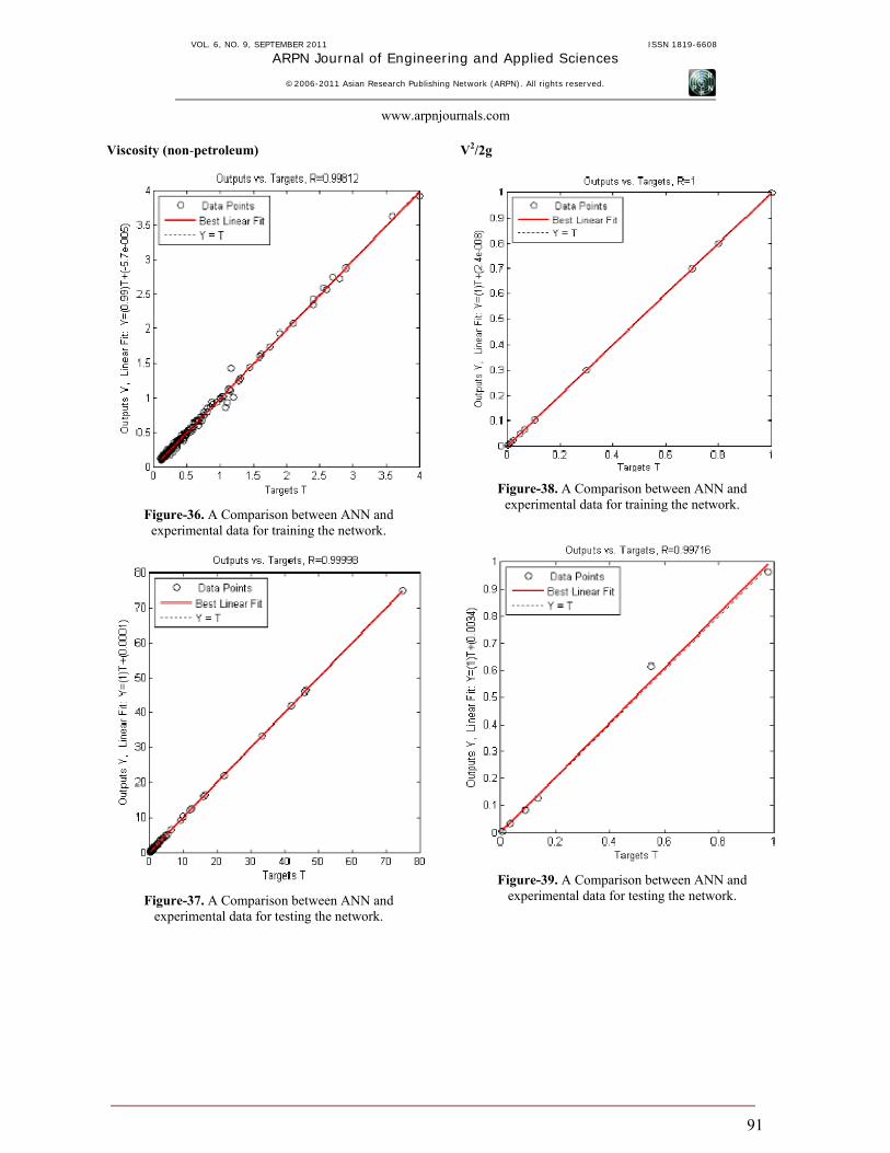
Viscosity (non-petroleum)
Figure-36. A Comparison between ANN and experimental data for training the network.
Figure-37. A Comparison between ANN and experimental data for testing the network.
V2/2g
Figure-38. A Comparison between ANN and experimental data for training the network.
Figure-39. A Comparison between ANN and experimental data for testing the network.
VOL. 6, NO. 9, SEPTEMBER 2011 ISSN 1819-6608
ARPN Journal of Engineering and Applied Sciences
©2006-2011 Asian Research Publishing Network (ARPN). All rights reserved.
www.arpnjournals.com
92
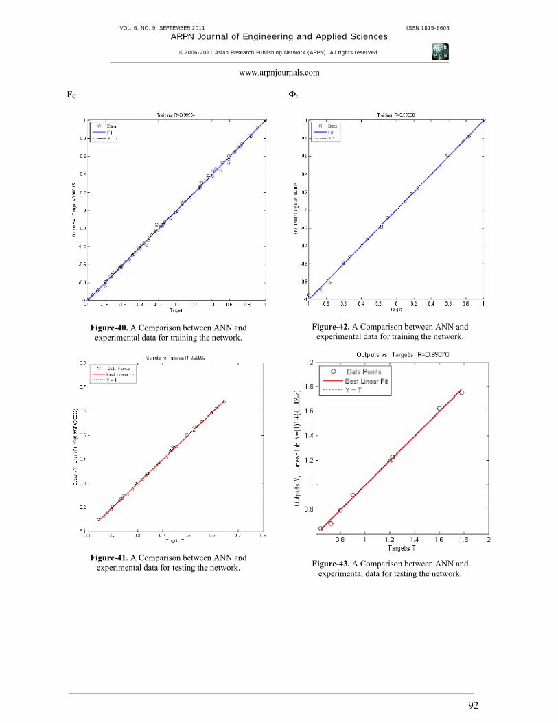
FC
Figure-40. A Comparison between ANN and experimental data for training the network.
Figure-41. A Comparison between ANN and experimental data for testing the network.
Фt
Figure-42. A Comparison between ANN and experimental data for training the network.
Figure-43. A Comparison between ANN and experimental data for testing the network.
VOL. 6, NO. 9, SEPTEMBER 2011 ISSN 1819-6608
ARPN Journal of Engineering and Applied Sciences
©2006-2011 Asian Research Publishing Network (ARPN). All rights reserved.
www.arpnjournals.com
93
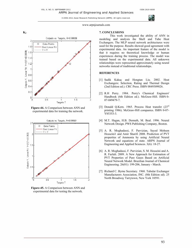
KC
Figure-44. A Comparison between ANN and experimental data for training the network.
Figure-45. A Comparison between ANN and experimental data for testing the network.
7. CONCLUSIONS This work investigated the ability of ANN in
modeling and analysis the Shell and Tube Heat Exchangers. The MLP neural network architectures were used for the purpose. Results showed good agreement with experimental data. An important feature of the model is that it requires no theoretical knowledge or human experiences during the training process. The model was trained based on the experimental data. All unknown relationships were represented approximately using neural networks instead of traditional relationships. REFERENCES [1] Sadik Kakaç and Hongtan Liu. 2002. Heat
Exchangers: Selection, Rating and Thermal Design (2nd Edition ed.). CRC Press. ISBN 0849309026.
[2] R.H Perry. 1984. Perry's Chemical Engineers' Handbook (6th Edition ed.). McGraw-Hill. ISBN 0-07-049479-7.
[3] Donald Q.Kern. 1965. Process Heat transfer (23rd printing 1986). McGraw-Hill companies. ISBN 0-07-Y85353-3.
[4] M.T. Hagan, H.B. Demuth, M. Beal. 1996. Neural Network Design. PWS Publishing Company, Boston.
[5] A. R. Moghadassi, F. Parvizian, Sayed Mohsen Hosseini1 and Amir Sharifi 2008. Prediction of PVT properties of Ammonia by using Artificial Neural Network and equations of state. ARPN Journal of Engineering and Applied Sciences. 3(6): 18-27.
[6] A. R. Moghadassi, F. Parvizian, S. M. Hosseini and A. R. Fazlali. 2009. A New Approach for Estimation of PVT Properties of Pure Gases Based on Artificial Neural Network Model. Brazilian Journal of Chemical Engineering. 26(01): 199-206, January - March.
[7] Richard C. Byrne Secretary. 1968. Tubular Exchanger
Manufacturers Association, INC. (8th Edition ed). 25 North Broadway Tarrytown, New York 10591.