Rochester Institute of Technology Rochester Institute of Technology

RIT Scholar Works RIT Scholar Works

Theses

2003

An Exploration of MPEG-7 Shape Descriptors An Exploration of MPEG-7 Shape Descriptors

Bret Woz

Follow this and additional works at: https://scholarworks.rit.edu/theses

Recommended Citation Recommended Citation Woz, Bret, "An Exploration of MPEG-7 Shape Descriptors" (2003). Thesis. Rochester Institute of Technology. Accessed from

This Thesis is brought to you for free and open access by RIT Scholar Works. It has been accepted for inclusion in Theses by an authorized administrator of RIT Scholar Works. For more information, please contact ritscholarworks@rit.edu.

An Exploration of MPEG-7 Shape Descriptors

by

Bret Woz

A Thesis Submitted

in

Partial Fulfillment of the

Requirements for the Degree of

Master of Science

in

Computer Engineering

Ad~sor: ______________________________________ __

Dr. Andreas Savakis, Associate Professor and Department Head

Co-Advisor: _____________________________________ __

Dr. Ricardo de Queiroz

Committee Member: _____________________________________ __

Dr. Fei Hu, Assistant Professor

Committee Member: ____________________________________ __

Dr. Greg Semeraro, Assistant Professor

Department of Computer Engineering

Kate Gleason College of Engineering

Rochester Institute of Technology

Rochester, New York

July 8,2003

Release Permission Form

Rochester Institute of Technology

An Exploration of MPEG-7 Shape Descriptors

I, Bret Woz, hereby grant permission to the Wallace Library of the Rochester Institute of

Technology to reproduce this thesis, in whole or in part, for non-commercial and non-profit

purposes only.

Date

Abstract

The Multimedia Content Description Interface (ISO/IEC 15938), commonly known to

as MPEG-7, became a standard as of September of 2001. Unlike its predecessors,MPEG-

7 standardizes multimedia metadata description. By providing robust descriptors and an

effective system for storing them, MPEG-7 is designed to provide a means of navigation

through audio-visual content. In particular, MPEG-7 provides two two-dimensional shape

descriptors, the Angular Radial Transform (ART) and Curvature Scaled Space (CSS), for

use in image and video annotation and retrieval.

Field Programmable Gate Arrays (FPGAs) have a very general structure and are made

up of programmable switches that allow the end-user, rather than the manufacturer, to

configure these switches for whatever design is needed by their application. This flexibly

has led to the use of FPGAs for prototyping and implementing circuit designs as well as

their use being suggesting as part of reconfigurable computing.

For this work, an FPGA based ART extractor was designed and simulated for a Xilinx

Virtex-E XCV300e in order to provide a speedup over software based extraction. The design

created is capable of processing over 69,4400 pixels a minute. This design utilizes 99% of

the FPGA's logical resources and operates at a clock rate of 25 MHz.

Along with the proposed design, the MPEG-7 shape descriptors were explored as to

how well they retrieved similar objects and how these objects matched up to what a human

would expect. Results showed that the majority of the retrievals made using the MPEG-7

shape descriptors returned visually acceptable results. It should be noted that even the

human results had a high amount of variance.

Finally, this thesis briefly explored the potential of utilizing the ART descriptor for

optical character recognition (OCR) in the context of image retrieval from databases. It

was demonstrated that the ART has potential for use in OCR, however there is still research

to be performed in this area.

Acknowledgements

There are many people I would like to thank for their help and contributions to this

work. In particular, I would like to thank my two advisors, Dr. Andreas Savakis and Dr.

Ricardo de Queiroz. I would also like to thank my committee members, Dr. Fei Hu and

Dr. Greg Semeraro.

I would also like to thank the following people:

Dr.Martin Lukowiak for his assistance in answering questions pertaining to the Xilinx

FPGA and the software utilized.

Jeremy Brown and Travis Brown for the use of their Linux systems during the devel

opment stages of the C++ software.

Douglas Hoffman for aid in learning IMpX, suggestions, computer help, proof-reading,

and late-night meals.

Cindy Harper for proof-reading, editing, comments and much encouragement.

Lon Highby for his aid in the development of the Visual Basic GUI.

Richard Tolleson for various computer related and non-computer related aid.

Jennifer Zenner for proof-reading, editing and for the L^LEXform.

Anne DeFelice for aid with administrative tasks.

Last, but certainly not least, I would like to thank my parents, Gregory and Paula Woz,

as well as my brother, Jason Woz. Their support and encouragement has been greatly

appreciated.

TABLE OF CONTENTS

List of Figures iii

List of Tables vi

Glossary vii

Chapter 1: Introduction 1

1.1 Description . . 1

1.2 Image Retrieval From Databases .... 2

1.3 MPEG-7 3

1.4 Overview . . . . . 4

Chapter 2: Introduction to Shape Description or Representation 6

2.1 Relevance to image databases . . .... 6

2.2 Overview of previous research and work in shape description or representation 6

2.3 Chain Code 11

Chapter 3: The MPEG-7 Shape Descriptors 14

3.1 The Angular Radial Transform . 14

3.2 Curvature Scaled Space . . .... . 18

Chapter 4: Software Implementations and Results 26

4.1 MATLAB Implementation 26

4.1.1 CSS . .29

4.1.2 ART 30

4.1.3 Discussion of Results 35

4.2 Character Matching . ... 38

4.2.1 C++ Coding 38

4.2.2 User Input 39

4.2.3 Cygwin 40

4.2.4 Results and Discussion 40

Chapter 5: Hardware Implementation of the ART Shape Descriptor 42

5.1 Overview 42

5.2 Design 43

5.3 Implementation Details ... 48

5.3.1 The ART STAT Module 48

5.3.2 Stage 1: The CORDIC Pipeline 49

5.3.3 Divider 54

5.3.4 ART Stage 2 57

5.3.5 The Summation Block 60

5.4 Operation of the Extractor . . . 62

5.5 Results 64

5.6 Parallelization of the Design . 69

Chapter 6: Conclusion 73

6.1 Closing Remarks 73

6.2 Areas for Future Research . . .74

Appendix A: Matlab Query Results 76

Appendix B: Character Matching Results 83

Appendix C: CD Contents 88

Bibliography 89

LIST OF FIGURES

2.1 Example of Contour Versus Region-Based Similarity 7

2.2 The Grid Method 9

2.3 (a) A Polygon and (b) its Turning Function 9

2.4 Centroid-Radii Method 11

2.5 Chain Code Directions 12

3.1 The Real Part of the Basis Functions 15

3.2 Contour Evolution and CSS 22

4.1 Handwritten'J'

used in Testing 41

4.2 Typeset'J'

used in the Database . . . 41

5.1 16-Bit Representation of ART Values . . . ... . .44

5.2 The ART_STAT Module . . 47

5.3 State Machine for STAT module 48

5.4 ART_STAT waveforms 49

5.5 VHDL ART Stage 1 Module 50

5.6 The pre-processor (left), CORDIC pipeline, andpost-processor (right) .... 53

5.7 Example Waveforms for Stage 1 55

5.8 Block diagram of the Divider . . 56

5.9 Waveforms for the divider 58

5.10 VHDL Stage 2 59

5.11 Art Stage 2 Waveforms 61

5.12 The Summation Block 62

5.13 The Summation Block Waveforms 63

5.14 The initial stages of Operation for the ART Extractor 65

5.15 Acquiring Coefficients from the ART Extractor 66

in

5.16 HOST-FPGA Interaction 67

A.l Human Matchings for kkl83 (No Particular Order) 76

A.2 Human Matchings for kkl88 (No Particular Order) 76

A.3 Human Matchings for kk458 (No Particular Order) 77

A.4 Retrieval results from kkl83 using CSS 78

A. 5 Retrieval results for kkl88 using CSS . 78

A.6 Retrieval results for kk458 using CSS ... ... .78

A. 7 Retrieval results for kkl83 using LUT based ART without filling ... .79

A.8 Retrieval results for kkl88 using LUT based ART without filling 79

A.9 Retrieval results for kk458 using LUT based ART without filling 79

A. 10 Retrieval results for kkl83 using the exact ART without filling ... 80

A. 11 Retrieval results for kkl88 using the exact ART without filling 80

A. 12 Retrieval results for kk458 using the exact ART without filling 80

A. 13 Retrieval results for kkl83 using LUT based ART with filling 81

A. 14 Retrieval results for kkl88 using the LUT based ART with filling 81

A. 15 Retrieval results for kk458 using the LUT based ART with filling .... 81

A. 16 Retrieval results for kkl83 using the exact ARt with filling 82

A. 17 Retrieval results for kkl88 using the exact ARt with filling .... 82

A. 18 Retrieval results for kk458 using the exact ARt with filling 82

B.l Examples of Handwritten Characters in the Database . . .83

B.2 Examples of Typeset Characters in the Database 84

B.3 Query for'A'

against handwritten characters . . .85

B.4 Query for 'C against handwritten characters ... .85

B.5 Query for'J'

against handwritten characters 85

B.6 Query for'A'

against handwritten and typeset characters 86

B.7 Query for lC against handwritten and typeset characters ... . .86

B.8 Query for'J'

against handwritten and typeset characters ... 86

B.9 Query for'A'

against typeset characters . . .. . 87

B.10 Query for 'C against typeset characters 87

iv

B.ll Query for'J'

against typeset characters 87

LIST OF TABLES

4.1 Explanation of a Sample Query ... 27

4.2 Top six human matches for kkl83 27

4.3 Top six human matches for kkl88 28

4.4 Top six human matches for kk458 . 28

4.5 Summary of the CSS Results .... 30

4.6 MATLAB Exact Coefficients versus LUT Calculated Coefficients 33

4.7 Summary of the ART Results 34

4.8 Summary of the MATLAB Results 35

4.9 Algorithm Comparison 37

5.1 Characteristics of the Implemented Extractor . 46

5.2 VHDL Computed Coefficients versus Exact Calculated Coefficients 70

5.3 VHDL Computed Normalized Coefficients versus Exact Calculated Normal

ized Coefficients . . .71

VI

GLOSSARY

ART: Angular Radial Transform, a region-based descriptor.

BINARY IMAGE: A black and white (bitonal) raster image consisting of pixels that are

either"on"

or "off".

CENTROID: The center of mass of an object given as an (x,y) coordinate pair.

CIRCULARITY: The ratio of an object's perimeter (P) to its area (A) as follows: circularity

ElA

CONTOUR-BASED DESCRIPTOR: A shape descriptor based on the boundary of an object.

CORDIC: COordinate Rotation Digital Computer An iterative technique for imple

menting mathematical functions such as multiplication, division, square root, sine,

cosine, and inverse tangent developed by Jack Voider.

CSS: Curvature Scaled Space: a contour-based descriptor.

DFT: Discrete Fourier Transform

ECCENTRICITY: The ratio of the major axis to the minor axis.

FD: Fourier Descriptor: a contour-based shape descriptor.

FLOOD FILL: A recursive method for filling an area with a particular color.

GUI: Graphical User Interface.

IEC: International Electrotechnical Commission.

VI 1

IEEE: Institute of Electrical and Electronics Engineers, Inc.

ISO: International Organization for Standardization.

LUT: Look-up Table.

MAJOR AXIS: The straight line segment that connects the two points of the boundary

that are farthest from each other.

METADATA: "data aboutdata"

,a descriptor of the content, quality, condition, and other

characteristics of data.

MINOR AXIS: Perpendicular to the major axis, its length is such that a bounding box

could be formed which just encloses the boundary.

MPEG: Moving Picture Expert Group.

MPEG-7: Multimedia Content Description Interface (ISO/IEC 15938): an international

standard for image metadata.

QBE: Query by Example.

QBIC: Query-by-Image Content, an IBM QBE Image Database.

RASTER IMAGE: An image that consists entirely of pixels laid out on a grid whose origin

is usually in the upper left-hand corner with the positive axes going to the right and

down.

REGION-BASED DESCRIPTOR: A descriptor that is based on how the pixels of an object

are distributed.

SQUID: Shape Queries Using Image Databases: A method of shape retrieval developed

at the University of Surrey, UK.

vm

TIFF: Tagged Image File Format: An image file format created by Adobe.

VHDL: VHSIC Hardware Description Language: A software language used for represen

tation of digital systems. IEEE Standards 1076-1987 and 1076-1993.

VHSIC: Very High Speed Integrated Circuit.

VOD: Video on Demand.

IX

Chapter 1

INTRODUCTION

1.1 Description

In recent years there have been major advances in digital imaging hardware, such as digital

photography and video, that have led to the expansion of the digital image world from the

professional and high-end consumer markets into the hands of everyday consumers. These

advances, combined with the increasing storage capacity of today's computers, have led to

databases consisting of hundreds or thousands of digital images. Such databases exist not

only on institutional or commercial servers, but also on everyday personal computers. With

databases of this size, manually sorting and searching through all of the images becomes

tedious. In order to efficiently automate these functions, the database must be able to

categorize and compare images using some form of metadata. It is preferable that this

metadata require little to no user intervention.

One of the challenges in the imaging world is the automatic extraction of semantic

labels of multimedia information [1] . Many systems developed for image retrieval use low-

level features such as shape, color, and texture [2]. These features can be further divided

into more specific categories. For example, the shape of the object can be divided into its

contour and the region of space it fills. All of these features can be extracted from an image

and converted into metadata usable in a system for image classification and retrieval.

These facts have led to the development of specialized tools and systems to aid in the

searching, storing, filtering, and managing of this information. Not only must these tools

work with data that has been previously stored, but also with live data being broadcast

through high-speed means such as digital cable. Frameworks have been proposed to pro

vide a means of interoperability for systems that generate, distribute, and consume this

information. Most notable among these is the effort by the Moving Picture Experts Group

(MPEG) which has become an international standard as of September 2001 [3].

1.2 Image Retrieval From Databases

Until the mid 1990s, most image databases based their queries on file IDs, keywords, or text

associated with the images [4]. While these search methods are powerful, they still require

human intervention in the form of determining what text and/or keywords to associate with

a given image. These associations are limited by the particular vocabulary used and are

prone to human errors.

In order to eliminate these problems, ongoing research has been performed in Query-by-

Example (QBE) image databases. A QBE image database is a database in which queries

are based on matching content to an example image in terms of texture, color, shape, etc.

This removes the majority of labor intensive tasks by human operators. Several like systems

have been developed, such as IBM's QBIC [4], Columbia University's Multimedia/VOD

testbed [5], and Surrey's SQUID project [6].

QBIC is a QBE image database designed to handle both still images and video. It

makes use of unsupervised segmentation and semiautomatic identification of objects in still

images. Automatic shot detection and representative frame choosing are also used [4].

QBIC performs a shape-based search by making use of features such as area, circularity,

eccentricity, moments, and major axis of inertia. When performing a search, QBIC takes

these features, creates a feature vector from them, and determines their similarity by using a

weighted Euclidean Distance metric. QBIC's search system is reliable when a small number

of objects are contained in an image and is sensitive to outliers [7].

Columbia University's Multimedia/VOD testbed makes use of texture, color, and shape

extractions [5]. The testbed also utilizes Euclidian Distance of its feature vector.

The SQUID system at the University of Surrey in the United Kingdom [6] is a shape-

based QBE image database. Its method for shape matching, Curvature Scaled Space, was

chosen as the basis for MPEG-7's contour shape descriptor. The SQUID system makes use

of locations of convex and concave sections of the contour for shape matching. Curvature

Scaled Space will be discussed in greater detail in Chapter 3.

Research into image databases continues on all levels, from the extraction and compar

ison of low-level features as in [8] to high level applications as in [9]. Effort has also been

given to standardize these features. One example of such work is the MPEG-7 standard.

1.3 MPEG-7

In July of 1996, MPEG initiated its standardization project. Following the same pro

cedures used in developing its previous standards, MPEG gathered representatives from

different sectors including software developers, manufacturers, service providers, broadcast

ers, academics and libraries. These groups then defined the context and objective as well

as identified the requirements of this new endeavor. Afterward, the group sent out a call

for proposals which were then evaluated. The end result is a recommendation outlined in

the final specification [3].

Known as the Multimedia Content Description Interface (ISO/IEC 15938), which is

commonly referred to as MPEG-7, this project differed from other MPEG standards such

as MPEG-1, MPEG-2 and MPEG-4. Instead of representing the content itself, such as

methods of compressing an image, MPEG-7 represents information about the multimedia

content, i.e. metadata. This standard provides robust descriptors and an effective system

for storing them.

MPEG-7 is divided into several sections [3]:

1. ISO/IEC 15 938-1: MPEG-7 Systems

2. ISO/IEC 15 938-2: MPEG-7 Description Definition Language

3. ISO/IEC 15 938-3: MPEG-7 Visual

4. ISO/IEC 15 938-4: MPEG-7 Audio

5. ISO/IEC 15 938-5: MPEG-7 Multimedia DSs

6. ISO/IEC 15 938-6: MPEG-7 Reference Software

7. ISO/IEC 15938-7: MPEG-7 Conformance

This thesis focused primarily on two of the shape descriptors presented in Part 3 of

the MPEG-7 standard. MPEG-7 provides two basic 2-D shape descriptors: a region-based

descriptor, called the Angular Radial Transform (ART); and a contour-based descriptor

designed around Curvature Scaled Space (CSS). Beyond examining these descriptors for

image retrieval, the major contribution of this thesis is a VHDL implementation of the

ART that is synthesizable to a field programmable gate array (FPGA).

1.4 Overview

The aim of this thesis is to explore the MPEG-7 shape descriptors, and propose a novel

hardware implementation of a FPGA base extractor for the ART descriptor. This requires

a familiarity with shape descriptors and with the MPEG-7 shape descriptors in particular.

It should be noted that the segmentation of images into individual objects falls outside the

scope of this work. It is therefore assumed that the segmentation of the image into binary

images each containing a single object has already been performed. The remainder of this

thesis is organized as follows.

Chapter 2, Introduction to Shape Metadata, provides a general overview of previous

work in shape metadata that is the basis for research today as well as current research in

shape description.

Chapter 3, The MPEG-7 Shape Descriptors, discusses in detail the two 2-D MPEG-7

shape descriptors, including how they are extracted and how distances between two ex

tracted descriptors are calculated.

Chapter 4, Software Implementations and Results, discusses the MATLAB implemen

tation of the ART and CSS shape descriptors. Also discussed is a C++ implementation

of the ART that is used for character retrieval. Results from trial matchings using these

systems are presented and evaluated.

Chapter 5, Hardware Implementation of the ART Shape Descriptor, explains in detail

the implementation of an extractor for the ART in a FPGA based hardware environment. A

comparison is made between results from the hardware implementation and the MATLAB

implementation.

Chapter 6, Conclusion, summarizes the accomplishments of this work, problems en

countered, and provides suggestions for future improvement, and possible future research

directions.

Chapter 2

INTRODUCTION TO SHAPE DESCRIPTION OR

REPRESENTATION

2.1 Relevance to image databases

When designing an image database to search for and retrieve similar images, it is desirable

for it to work such that the results make sense to the human user. For example, suppose a

cat and a brick are placed in front of a person and he/she is asked if they are the same and

why. Color would be one important factor; the cat is grey while the brick is red. Size could

be another differentiating factor; the cat is larger than the brick. The person may comment

on the texture of the two objects; the cat looks soft and the brick looks rough. Most likely,

the first observation would be that the cat and the brick have different shapes.

The shape of an object is strongly linked to that object's functionality and identity.

leading to shape features being very powerful when used in similarity search and retrieval.

Since shape alone can be used by a human to identify a characteristic object, it is known that

shape often carries semantic information. Shape-based recognition, retrieval and indexing

have been large areas of research [10].

2.2 Overview of previous research and work in shape description or represen

tation

Two ways are commonly used to compare similarity between two shapes. The first is to

determine that the outlines of the shapes are similar. For example, whether they both have

concave or convex curves at the same relative locations. This type of comparison us called

contour-based. The second is to note that the two shapes appear to have similar pixel

distributions. This is referred to as a region-based comparison. Both categorizations are

best demonstrated in Figure 2.1 [11]. In this image, shapes in the same row can be said to

have regional similarity whereas the images in the same column can be said to have similar

contours.

s

5

i i

rig

6 laFigure 2.1: Example of Contour Versus Region-Based Similarity

Many different ways have been developed to represent shapes for both region and con

tour matching. Region-based methods include moments [12] and grid-based technique [13].

Contour methods include turning angles [14], Fourier Descriptors [15], and centroid-radii

(cited in [8], published in [16]) on which distance histograms [8] are based. The region-based

methods will be examined first, followed by the contour based methods.

Moments are one descriptor that can usually be found in an image processing textbook

such as [17] and are based upon work done in [12]. The moments of an N x M binary

image f(x,y) are defined as:

m

M-17V-1

The mean x and y coordinates of the object, known as the center of gravity or centroid, in

the image can be calculated by:

mii0x =

mo,o

and

m0,iy-

In these equations, mo,o is the area of the object, my and mn,i are the sum of the x and

y coordinates respectively. Using these centroid coordinates, the central moments of the

image can be determined in the following manner:

M-1N-1

wj= 5Z !>2(x-xY(y-yy

y=0 Z=0

From these equations, it is possible to determine the major axis of the object relative to its

x-axis and the size of the object in the x and y directions. A set of seven invariant moments

can be created from the second and third order moments [12]. These moments are invarient

to changes in translation, rotation and scale.

In the grid-based method [13], an object is placed on a grid. The squares of the grid

that the object wholly or partially covers are assigned a number '1', while the other squares

are assigned a number '0'. The grid is then traversed from left to right in a top to bottom

order to obtain a string of numbers that can be used to describe the image. For example.

the shape in Figure 2.2 [13] would produce the string 001111000 011111111 111111111

111111111 111110111 011100000011. The difference between two shapes can be calculated

by determining the number of grid squares covered by one shape, but not by the other. This

simple method is invariant to translation and, with a few further modifications, can make

the method unaffected by scaling and rotation as well.

Turning angles [14] is the first of the contour-based methods to be discussed. This

method makes use of a turning function, 9a{s), that measures the angle of the counter-

clock-wise tangent as a function of the arc-length as measured from a starting point on

the contour. The value of the turning function is the angle that the tangent at this point

makes with the x-axis (or a predetermined reference axis). As the contour is traversed, the

value of the turning function will increase with left-hand turns whereas right hand turns

! /XX-X^ i j i

1 / i T^fs^y ; I : : i i I

%

Figure 2.2: The Grid Method.

will decrease its value. This can be seen in Figure 2.3 [8] where in (a) O is the starting

point and in (b) the turning angles can be tracked. Assuming that two polygons with their

contours normalized to 1 exist, the distance between two turning functions 0a(s) and 6b{s)

is defined as:

D{A,B) = minr,g{ fe20A(i)-6B(

where minr^ is the minimum value of rotation and shifting of polygon B. This descriptor

is invariant to translation and scale. It can also be made invariant to rotation.

Figure 2.3: (a) A Polygon and (b) its Turning Function

Fourier Descriptors [15] are contour-based descriptors that have been around for many

years. The basic premise is to treat a 2-D signal such as an object contour as a 1-D signal.

This is achieved in the following manner [17]:

1. Start with a contour consisting of coordinates d(i) = [x(i), y(i)] for i = 0 to N-l

2. Treat these points as a complex number so that s(k)=

x(k) + jy(k)

3. Perform the Discrete Fourier Transform (DFT) on s(k) to create a(u):

A/-1

Ma(u)

=

77 H s(k)e^

fc=0

FDs are affected by geometric transformations in the following ways [18]:

Translation: Translating s(k) in space corresponds to scaling the u=0 term of a(u)

s(k) + a <-> a(u) + ad(u)

Scaling: Scaling s(k) by 8 scales the FDs by 8.

Bs{k) <x=> Ba(u)

Changing the Origin: Changing the Origin modulates a(u).

s(k ko) & M

Rotation: If the points are rotated by 0, then s(k) goes tos(k)eJ'e

s(k)eje

<t=>a{u)ej0

In the centroid-radii method [8] [16], the lengths of the radii from the centroid of an

object to its boundary are used to describe the shape. The number of radii, k, is determined

by the angle, 0, in degrees, as shown in the following equation:

10

Figure 2.4: Centroid-Radii Method

This can be seen in Figure 2.4 [8].

The vector of radii is:

VECradii = {Lq, Lg, L2g, ..., (fc-l)#)

This is divided by the largest radii to make it invariant to scaling to become:

Two shapes, 11 and 12, match only if their corresponding radii are below some minimum:

\\lli9 -

12W\\ < MRDTVie[0, k -

1]

where MRDT is the maximum radius difference tolerance.

The distance histogram method [8] is very similar to the centroid-radii method. First,

the centroid is calculated. Next, each side of the boundary is resampled n times, where n is

relative to the length of the side. The radii to these points are calculated and a histogram of

the distances formed. The similarity between the two histograms is measured by Euclidean

Distance [8].

2.3 Chain Code

Chain codes are one way to represent a boundary. The process is as follows [17]:

11

2

3. T A

4*

/5

b

Figure 2.5: Chain Code Directions

1. Specify a starting point on the boundary. Record the point coordinates.

2. Beginning in Direction 0 (refer to Figure 2.5), rotate counter-clockwise through the 8

pixels surrounding the current pixel until the next pixel in the boundary is found.

3. Record the location of the next pixel and move to it.

4. Begin the search again starting one pixel counter-clockwise of the direction to the last

pixel. For example, if the direction of the last pixel is one pixel to the left and one

pixel up (Direction 3), start the search one pixel to the left (Direction 4)).

5. Repeat steps 3 and 4 until either:

The initial pixel started at is reached.

The direction of the next pixel is the same as the direction of the last pixel. For

example, if the algorithm reach a point on the contour where the only choice it

has is to move to the pixel it was just at.

Usually a chain code is the list of directions that are taken while traversing the boundary.

For example: [0,0,3,4,4,1] would be the chain code for a simple 3x2 pixel rectangle. This

type of representation is best when using chain codes as a descriptor, but requires processing

if the user wants exact pixel locations. For this thesis, the coordinates were recorded to

save processing time.

12

Having explored previous and current research into shape metadata, the next chapter

examines one of the latest developments in shape metadata, the MPEG-7 standard.

13

Chapter 3

THE MPEG-7 SHAPE DESCRIPTORS

3.1 The Angular Radial Transform

MPEG-7's region-based shape descriptor is based upon multiple complex-valued orthonor-

mal 2-D basis functions that are defined by the Angular Radial Transform. A shape is then

mapped onto these basis functions and the coefficients produced are normalized and then

used to describe the shape [10].

As seen in [10], the ART is based in a polar coordinate system where the sinusoidal basis

functions are defined on a unit disc. Given an image function in polar coordinates, f(p,0),

an ART coefficient Fnm (Radial order n, angular order m) can be defined as:

Fr, = (vnm(p,0)j(P,0)) = r f (v:m(p,0)f(p,0)p)dpd0Jo Jo

Vnm(p, 0) is the ART basis function and is separable in the Angular and Radial directions

so that:

Vnm(p,0) = Am(0)Rn(p)

The angular basis function, Am, is an exponential function used to obtain rotation invari-

ance. This function is defined as:

Am(0) = -\-^

Rn, the radial basis function, is defined as:

1 if n = 0

Rn{p) = .

2cos{-Knp) if n / 0

14

MPEG-7 makes use of twelve angular and three radial functions. The real parts of these

basis functions can be seen in Figure 3.1.

m 0 1 2 3 4 5 6 7 8 9 10 11

i^KSK9B9Z9E'1 p

*'l*

*LAwmPJ. I

Figure 3.1: The Real Part of the Basis Functions

It is shown in [19] that the magnitudes of the ART coefficients are invariant to rotation

in the following manner: Assume that there exists a polar image function f(p, 0) and a

rotated version of this function fa(p, 0) where a is the angle of rotation around the origin.

So

fa(p,0) = f(p,a + 9)

Then the ART of the rotated image is:

Km =

7r\ \ {VnmiP, VfXP, O)p)dpd027T JO JO

This can also be written as:

Hence:

-Trim1 nmc

nm~

-1 nm

In order to achieve scaling normalization, the magnitude of each coefficient is divided

by the magnitude of the n=0, m=0coefficient. The coefficient is equivalent to the area of

the shape.

15

Four basic steps exist to extract this descriptor from an image [20]. The first step is

to generate a look up table (LUT). This table is used to enhance the speed of coefficient

extraction by reducing the amount of computations that must be performed. Since the basis

functions are separable, rather than compute Vnm(p,9) in polar coordinates and converting

it to Cartesian coordinates, it is easier to compute Vnm directly in Cartesian coordinates. To

do this, two 4-dimensional arrays, BasisR and BasisI, are created, each of which respectively

contain the real and imaginary components of Vnm. In the following steps, LUT.SIZE is

the size of the look up table. LUT.SIZE is typically 101 [20].

Given the center of the LUT is (CX,CY), for every (x,y) coordinate in the LUT perform

the following steps:

1. r = sqrt(x ex) * (x ex) + (y cy) * (y cy);

2. 0 = arctan*=Sixcx

3. For every m and n, where 0 < m < 11 and 0 < n < 2

(a) temp = cos

^lXXsize^

(b) The real part of the value (m,n) for LUT coordinate (X,Y) is: temp cosm0

(c) The imaginary part of the value (m,n) for LUT coordinate (X,Y) is: temp-smm0

Parts 1 and 2 above convert the Cartesian coordinate (x.y) into polar coordinate (r,6>).

Part 3 calculates the LUT value for the 12 angular, m, functions and 3 radial, n, functions.

Temp is the value in the radial direction. Steps (b) and (c) calculate the values in angular

direction and combine them with the value in the radial direction. This produces the LUT

value for the (X,Y)

pair. Two separate LUTs are created, one for the real part of the ART

and one for the imaginary part of the ART, of size LUT.SIZE x LUT_SIZE x 12 x 3.

16

Step two consists of normalizing the size of the object in question. First, the size of

the object must be defined as twice the maximum distance from the centroid of the object

to its edge. This is done so that the object can be properly scaled to the LUT. Next, the

centroid of the object is aligned with the center of the LUTs. Assume that an image, i,

exists containing an object, 0, that has a maximum radius of MAX.OBJJIADIUS and a

centroid at (OCX, OCY). For every point (X,Y) that is contained in O, map the image in

the following manner:

iqrnlp

_ LUT.RADIUScutc

MAX.OBJ.RADIUS

2. dx = X-OCX

3. dy = Y-OCY

4. nx = scale dx + LUT.RADIUS

5. ny= scale dy + LUT.RADIUS

Where LUT.RADIUS =[LUT-!=IZE

\.

In step three, the real and imaginary parts of ART coefficients, ArtR and ArtI, are

computed after mapping is performed. These are matrixes of size 12x3 where entry is the

sum of all pixels in the lookup table that correspond to a pixel in the image. For this thesis,

all images were binary and had white backgrounds [pixel value = 1] and black objects [pixel

value = 0].

For ever 0 < m < 11 and 0 < n < 2 the real and imaginary values for the ART must

be retrieved from the corresponding LUT. The retrieved real value is added to the current

value of ArtR while the retrieved imaginary value is subtracted from the current value of

ArtI. Which entry to retrieve from the LUT is determined by nx and ny. Should nx and/or

17

ny not be integer values, then the value to be added for a given n and m must be linearly

interpolated from the surrounding entries in the LUT.

Finally, the magnitude of each coefficient, ArtM(m,n), is calculated. For each m and

n, this value is defined as:

ArtMagnitude(m,n) =^(ArtR(m,n))2

+(Artl(m,n))2

The individual values that are calculated are then normalized by dividing by the zeroth

coefficient. This coefficient is equal to the area of the object being transformed and dividing

by it allows for scale invariance in the ART. For each m and n:

,,. ArtMaqnitude(m.ri)

ArtM(m.n) = \'

ArtMagnitude(0, 0)

At this stage, MPEG-7 performs quantization of the normalized coefficients in order

to create a size efficient descriptor. As it was not the intention to implement the System

Architecture and Description Definition Language defined in MPEG-7, quantization was

left out of the thesis.

The distance between two ART descriptors, ArtMA and ArtMs, is an Li distance (also

known as Manhattan distance) between the two sets of normalized values:

35

Distance(A, B) - ^ \ArtMA{i)-

ArtMB(i)\i=0

This ends the description of the MPEG-7 region-based descriptor. The next section will

examine MPEG-7's contour-based descriptor.

3.2 Curvature Scaled Space

The second of the 2-D shape descriptors in the MPEG-7 standard is the contour-based shape

descriptor, which occupies the Curvature Scaled Space (CSS). The contour-based method

was originally developed by Farzin Mokhatarian, et al., at the University of Surrey and was

further refined for use in the MPEG-7 standard.

18

It has been observed that humans tend to break the contour of a shape into concave

and convex sections when comparing with other shapes [10]. They then use the similarity

of these individual sections to determine the similarity of two contours. Comparisons such

as relative length, position in the contour, and the order in which they occur in the contour

may be used.

CSS uses a similar technique. It also segments the contour into convex and concave

sections by calculating the points in the contour where the curvature is zero. The contour is

then slowly smoothed out by means of filtering, with each inflection point being monitored

throughout the filtering process. When a section of the contour becomes completely convex,

the number of times filtering occurred and the location relative to the start of the contour

for the center of the section are recorded. These pairs of location and number of times

the filter was applied become the basis for the descriptor. Filtering stops when the whole

contour becomes convex. The benefits of this descriptor are that it is robust both to noise

and to differences in scale and orientation.

The following is a more detailed explanation of the process of descriptor extraction [20].

First, assume that a contour Q exists such that:

n = {(X0,Y0),(XuY1),...,(Xn,Yn)}

Where (Xn,Yn) are the coordinates of the points contained in the contour. These pointsare

then used to construct the functions X(u) and Y(u), where u is the arc-length of the contour

normalized to be in the interval [0,1]. Next, these functions are resampled to consist of N

equidistant points. Usually N = 256 gives adequate results [20]. The resampled functions

are x(j) and y(j), where j is an integer index in the range [0,iV-l]. It is these resampled

functions that will be filtered. After each filtering, the curvature at any given j can be

19

calculated using the equation:

Xu(j, k)Yuu(j, k)-

Xuu(j, k)Yu(j, k)KU,k) =

(Xu(j,kY +Yu{j,k)2

Where

and

Xu(j,k) = X(j,k)-X(j~l,k)

Xuu(j, k) = Xu(j, k) -Xu{j-1, k)

Xu and Xuu represent discrete approximation of the first and second derivatives of X.

Similar formulas are used for Yu(j, k) and Yuu(j, k). In these equations, k is the number

of times that the points have been filtered. Zero crossings in the curvature can be found

when K(j, k)K(j 1, k) < 0. If the value of K(j, k) is non-negative then the corresponding

point is considered to be part of a convex segment of the contour. Otherwise, the point is

considered to be part of a concave section of the segment [17].

The general algorithm for determining the peaks and converting them to the CSS format

is as follows [20]:

1. Extract equidistant contour pixels from the region/object. Create an empty set of

peaks for the CSS image.

2. Create arrays of dx, dy data, where dx is the change in X-coordinate around the shape

contour boundary between pixels and dy is the change in Y-coordinate around the

contour.

3. Calculate the curvature function for each position on the boundary.

4. Find zero crossings in the curvature function. These zero crossing points are the

current set of minima and maxima on the contour shape boundary.

20

5. Compare the current set ofminima and maxima with those from the previous iteration.

If the current set is smaller than the previous set, there must be peaks that have

dropped out of the dataset.

6. For all minima and maxima in the current dataset, remove the corresponding minima

and maxima from the previous dataset. This will leave a set of minima and maxima

removed by filtering at this iteration.

7. Find the midpoint between the remaining minima and maxima. This corresponds to

the x.css coordinate of a peak; the y.css coordinate is the recursion number.

8. Insert this peak to the current set of peaks, ordered by recursion. If there are more

than 64 peaks after insertion of this peak, remove the smallest and most insignificant

peak from the set.

9. Filter the dx, dy sets of data using a low pass filter with the kernal [0.25, 0.5, 0.25].

This filter causes the contour of the object to slowly smooth out towards the final

state of being an ellipse where there is no change in curvature.

10. Repeat steps 5 through 9 until there are no minima and maxima remaining.

11. When all peaks have been found, map the x.css coordinates of each peak onto the

relevant position on the final filtered shape. Also, re-scale these coordinates to lie in

the range [0.0, 1.0]. The rescaled coordinates of the peaks are referred to as xpeak(i).

12. Now transform these peaks.

Transform all peak heights according to the equation ypeak[i]= 3.8 -($s^ )0,6;

samples

where Nsarnpies is the number of equidistant points from the contour used for

smoothing.

21

Shift all peaks so that the highest peak after transformation is at the x.css

coordinate 0.0. Doing this makes the descriptor invariant to starting point on

the contour.

If the highest peak has a height of less than 0.09, remove all peaks.

For any peaks which have a height of less than ypeak(0)*0.05, remove them.

original contour

Figure 3.2: Contour Evolution and CSS

The building of the CSS image can be seen in Figure 3.2 [11]. To this list of peaks

and their normalized distances on the contour the circularity and eccentricity of both the

original and the smoothed contour are added. Circularity is defined as the ratio of an

object's perimeter P to its area A as follows:

P2

circularity=

A

The circularity of an object shows the complexity of its boundary. [21] A high circularity

value means a more complex boundary. For example, consider a circle and a square.

For the circle:

A =irr2

22

For the square:

2-nr

,.

(2irr)24^V

circularity= - = = Air

A =s2

P = 4s

.

,.

(4s)2 16s2

circularity= ^ = - = 16

s2 s2

Where s is the length of one of the sides of the square. As it 3.14, then 4-7r 12.56 < 16.

This shows that a square is more complex than a circle.

The major axis of a boundary is the straight line segment that connects the two points

of the boundary that are farthest from each other. Perpendicular to the major axis is the

minor axis. Its length is such that a box could be formed that just encloses the boundary.

The ratio of the major axis to the minor axis is called the eccentricity. It is calculated in

the following manner [17]:

eccentricity

0.5(i2o + 202) + 0.5v/i2o +%_ 2i2002 + 4if j

\ 0.5(i2o + 202)-

0.5^20 + *02_ 2i2oi02 + 4ifi

Where:

TV

*02= Yl^i~ y^2

i=0

TV

\2

120= X^(Xi ~~

Xc)

i=0

TV

n= ^2(xi-xc)(yi -yc

i=0

(xi,yi) are coordinates of the points in the boundary and (xc, yc) are the coordinates of the

centroid of the object. N is the number of points in the boundary.

23

Matching of two contour shape descriptors is done as follows:

First, the following equations must be true:

\cq(0)-

Cr(0)\^

max(ca(0),Cr(0))

Ml) -Cr(l)< Thr

max(cq(l),Cr(l))

Where cg(0) and Cr(0) are the eccentricity of the query and the reference object respectively,

and Cq(l) and cv(l) are the circularity of the query and reference shape respectively. The

and Thc are thresholds and were set to 0.6 and 1.0 respectively as done in the MPEG-7

standard.

Once these conditions are met, further comparisons can be made. The distance between

two contour descriptors is as follows:

dlst = o 4 .

MQ)-^()I+ 03 .

\cg(l) -

cr(l)\+ Mcgs

max(cq(0),cr(0)) max(c(?(l),cr(l))

Where

Mess = ^2((xpeak(i) -

xpeak(j))2

+ (ypeak(i)-

ypeak(j))2) +^(ypeak(i))2

l 2

3 1is the summation over all match peaks and YI2 *s tne summation over all unmatched

peaks. In order to be considered matched, the L2 distance (Euclidean Distance) between

the x-coordinates of the two peaks must be less than 0.1.

It is possible to have a continuous segment of a query contour that matches a continuous

segment of a reference contour. This being the case, it is necessary to attempt to match up

these corresponding segments. It is also necessaryto take into account that the object may

be mirrored. As such, all peaks should also be mirrored by setting xpeak(i) = 1 xpeak(i).

To compensate for these two facts, a straightforward pattern matching algorithm is used to

find the minimum value for Mess (Based upon the algorithm found in [22]):

24

1. Create a mirrored copy of the query vector.

2. Match up peaks for both of the query vectors to the reference vector and calculate

Mess.

3. Rotate both query vectors so that the next peak is located at point 0.0.

4. Repeat steps 2 and 3 until the query vectors have returned to their original states.

5. Rotate the reference vector by 1 peak.

6. Repeat steps 2 through 5 until the reference vector has returned to its original state.

This algorithm is the equivalent of rotating two objects until corresponding curves in

the contour of each object are in relatively the same spacial positions.

25

Chapter 4

SOFTWARE IMPLEMENTATIONS AND RESULTS

4.1 MATLAB Implementation

The first step in this thesis was to implement and study the shape descriptors. MATLAB

provides an environment that has both basic and advanced math functionality, imaging

packages and functions for file input and output. These features made MATLAB an ideal

way to implement prototypes for each of the three descriptors.

The next several sections discuss the three descriptors and how they were implemented

in MATLAB. The test input consisted of 1,100 images of fish contours that were obtained

from [6]. Each image was provided as a list of points that made up the contour of the image.

The points were plotted in an 8-bit image file, where the background was white (pixel value

of 255) and the object points were black (pixel value of 0). For ease of use with MATLAB.

the images were then stored as 8-bit uncompressed TIFF files. The individual descriptors

were extracted and written out to files to be read in as metadata when searching through

the database for matches.

Each descriptor was tested in several ways to examine what conditions would provide

closer matches. Curvature Scaled Space will be discussed first followed by the ART. All

MATLAB code can be found in Appendix C on the included Compact Disc.

In each section, sample queries are presented. For each sample query, the image in

the upper left-hand corner is the query image. This image is one of the images contained

in the database and is not considered when searching for a match. The other six images

following the query are images that the algorithms determined were the best matches for

26

Table 4.1: Explanation of a Sample Query

Query Image

Closest Match Match 2 Match 3

Match 4 Match 5 Match 6

Table 4.2: Top six human matches for kkl83

Flank Subject 1 Subject 2 Subject 3 Subject 4 Subject 5

1 kk79 kkl81 kkll kkl81 kkl86

2 kkl81 kk79 kkl81 kkl86 kk79

3 kkll kkll kk79 kk67 kkl81

4 kkl86 kkl86 kk67 kk69 kk69

5 kk73 kk67 kk73 kk73 kkll

6 kk69 kk69 kkl86 kk79 kk67

that descriptor, in descending order (as seen in Table 4.1). The value above each image is a

score for how well it matches against the query image on a scale of 0.0 to 1.0, where 0.0 is

an exact match and 1.0 is farthest away from matching. This value is obtained by mapping

the distance value given from the descriptors to the normalized scale.

Five people were asked to pick what they consider the closest matches for each query

image shown. This was done by presenting the subject with a query image. Then they

were presented with visually acceptable matches from the database, (30 to 60 depending on

the image), and asked to list what they thought were the top six matches for that image,

ranked from closest to farthest. The three query images used were kkl83.tif, kkl88.tif, and

kk458.tif, which were selected at random from the database of images. The results for each

image are given in Tables 4.2, 4.3 and 4.4. These matchings are seen in Figures A.l, A.2,

and A.3.

As can be seen in the tables, not only do the human rankings of the closest images differ,

27

Table 4.3: Top six human matches for kkl88

Rank Subject 1 Subject 2 Subject 3 Subject 4 Subject 5

1 kklOO kkl89 kklOO kklOO kklOO

2 kklOl kkl02 kklOl kklOl kk310

3 kkl75 kklOO kkl02 kkl035 kklOl

4 kk807 kklOl kk304 kkl56 kk553

5 kkl035 kkl75 kkl30 kkl30 kkl75

6 kk651 kk99 kkl89 kkl034 kkl56

Table 4.4: Top six human matches for kk458

Rank Subject 1 Subject 2 Subject 3 Subject 4 Subject 5

1 kk456 kk456 kk453 kk327 kk456

2 kk455 kk455 kk456 kk462 kk453

3 kk452 kk452 kk462 kk456 kk462

4 kk327 kk454 kk9 kk455 kk36

5 kk454 kk460 kk449 kk462 kk724

6 kk564 kk6 kk454 kk328 kk449

28

but in two of the cases, so do the images listed. This shows that there is significant variation

in the human responses. This being the case, each query will be evaluated in two ways.

The first method is to count how many of the images returned from a query match up with

the images in the corresponding human results. The second method is to count how many

of the returned images are visually acceptable. This involved ascertaining whether major

features of the object retrieved corresponded to features found in the query image. Some

examples of the features considered include locations and number of fins, curves, and bends

as well as the shape of these and other features such as mouths and heads.

With these definitions, the next section will discuss CSS.

4.1.1 CSS

The extraction of the Curvature Scale Space descriptor started with the extraction of the

contour points using the chain code method. These points were then resampled and the

CSS descriptor was extracted using the algorithm described in Section 2.3. During this

extraction, the zero crossings for the curvature were located at the point where the curvature

actually changed from being positive to negative. For example, if the curvature clearly was

positive at one point and negative at the next, this was considered a zero crossing.

The special cases where the curvature leveled at zero before switching signs, or did not

switch signs at all, were dealt with in the following manner. To illustrate how these were

handled, assume that the current value for the curvature is positive and the next value for

the curvature is zero. The code examines the points until either a negative value is found, a

positive value is found, or it returns to the current point, (the list of points is treated like a

circular buffer). If a negative value is found, the current value is considered a zero crossing.

If a positive value is found or all the remaining values are zero, then a minimum is found.

The same is essentially true when the initial value is negative, except that the algorithm

now looks for the next value to be positive. If such a value is found, this point is considered

29

Table 4.5: Summary of the CSS Results

kkl83 kkl88 kk458

Matches with Human Results

Visually Acceptable

4

6

2

6

4

5

a maxima.

The mapping of the distance for each image in the database to the range of 0.0 to 1.0

was created after it was heuristically determined that the majority of the distances were

less than 2.0. This lead to the mapping being:

ClippedDistance =Distance If Distance < 2

2 Otherwise

ClippedDistanceM appedDistance

This mapping gives the normalized distance for the returned image. The CSS descriptor

were extracted using the MPEG-7 recommended resamping of the contour to 256 points.

Figures A.4, A.5 and A.6 show the results from queries using kkl83.tif, kkl88.tif, and

kk458.tif. Table 4.5 summarizes the results from the queries. The results will be discussed

and compared with the ART descriptor in Section 4.1.3. The next section presents the

ART, MPEG-7's region based descriptor.

4.1.2 ART

The ART was the second descriptor to be implemented. The tests for the ART varied in

two ways. First, the image was either just the empty fish contour, or the contour was filled

using the polygon fill method described in the following section and the ART descriptor was

extracted from the object created. The second test variation was that the descriptor was

either extracted using the LUT method, as described in the MPEG-7 standard, or it was

30

extracted using an exact calculation of the descriptor from the image points.

Polygon Fill

There are several ways to fill an object. One of the least complex of these methods is a flood

fill. In a flood fill, a starting pixel is chosen and set to the fill color. The neighboring pixels

are then checked to see if they are"on"

(For this thesis "off", or background, pixels are set

to the value for white and"on"

pixels set to black). In the case of a 4-neighborhood flood

fill, these would be the up, left, right, and down pixels. In the case of an 8-neighborhood

flood fill, it would be all eight surrounding pixels in either a clockwise or counter-clockwise

direction for both cases. For each"off"

pixel, one would move to that pixel, turn it "on",

and begin to check its neighborhood. Any"on"

pixel would be ignored and skipped. This

algorithm is very straightforward to implement recursively.

A flood fill is effective when the interior of an object is undivided and the location of a

position inside the object is known. When it is uncertain where a position inside the object

may be or if the contour of the object is shaped in a way that the interior consists of one or

more individual"hollow"

areas, a different type of fill would be more effective. Also, a flood

fill would not be effective in the case where one only knows the vertices of the object to fill

instead of a complete contour. In this case, the flood fill would fill the whole image with a

particular color. For this thesis, a polygon fill, also known as a scanline fill, was used. The

algorithm was taken from [23].

To execute a scanline fill, start at the top of the image and begin each scanline from left

to right, starting at the top scanline that the object is a part of and moving downward to

the lowest scanline ofwhich the object is a part. When a boundary of the polygon is reached

or crossed, set the pixel to thefill color and continue to set all pixels after the boundary to

the fill color until another boundary of the polygon is reached or crossed.

While traversing a scanline, instead of starting at the first pixel and checking each

31

individual pixel for an edge, precalculation of all the intersection points of the edges with

this scanline can be done. As only the vertices of the object are known, these intersection

points may not be integers so they are rounded to the nearest integer value. This will

always provide an even number of integer-valued intersections with a precision of +/- 0.5

pixel. To fill the scanline, a horizontal line is drawn from the first intersection to the next

intersection. Then, move to the next intersection, and repeat drawing and moving until all

intersection pairs have been used.

This is a straightforward version of the algorithm. A more complete version can be

found in [23] under the section polygon filling.

ART Matching Results

There were some differences between the LUT method and the exact calculation method of

the ART, but these differences are relatively minor after normalization. Table 4.6 shows the

differences between the exact and LUT normalized coefficients for image kk458.tif. These

values were obtained from the filled contour of the image.

As can be seen in the table, the maximum difference between the LUT method and the

exact method of calculating the descriptor is 0.006315, with the majority of the differences

being below 0.001. Testing indicated that the differences between the LUT method and the

exact values are due to the use of linear interpolation to determine the value of a non-linear

function, (as done in the LUT method). Examination of the sample queries, though, shows

that these differences are not enough to affect the top six matches.

After it was heuristically determined through testing that the majority of the distances

were less than 6.0, a maximum distance of 6.0 was imposed. Once more the distance was

mapped to the range 0.0 to 1.0:

Distance If Distance < 6

ClippedDistance

6 Otherwise

32

Table 4.6: MATLAB Exact Coefficients versus LUT Calculated Coefficients

n, m Exact Coefficients LUT Coefficients \Difference\

0,0 1 1 0

0,1 0.076869 0.076298 0.000571

0,2 0.530943 0.531753 0.000810

0,3 0.111480 0.112685 0.001204

0,4 0.327402 0.328232 0.000830

0,5 0.061106 0.060836 0.000270

0,6 0.188061 0.189032 0.000971

0,7 0.087303 0.087675 0.000372

0,8 0.188564 0.193739 0.005175

0,9 0.108372 0.108377 0.000005

0,10 0.130880 0.132071 0.001191

0,11 0.064561 0.064813 0.000251

1,0 0.175876 0.176157 0.000281

1,1 0.103664 0.103148 0.000515

1,2 0.140588 0.140520 0.000068

1,3 0.163552 0.164596 0.001044

1,4 0.096629 0.095842 0.000787

1,5 0.102438 0.103310 0.000871

1,6 0.073777 0.074289 0.000512

1,7 0.107493 0.107490 0.000003

1,8 0.042455 0.036140 0.006315

1,9 0.070660 0.071549 0.000889

1,10 0.056451 0.056811 0.000360

1,11 0.049000 0.049294 0.000293

2,0 0.139119 0.138932 0.000188

2,1 0.112886 0.113640 0.000753

2,2 0.222679 0.222675 0.000004

2,3 0.142052 0.141838 0.000214

2,4 0.148140 0.149387 0.001247

2,5 0.108403 0.108093 0.000310

2,6 0.145713 0.146396 0.000683

2,7 0.051876 0.052606 0.000731

2,8 0.125579 0.122547 0.003032

2,9 0.006114 0.005484 0.000629

2,10 0.037994 0.038611 0.000617

2,11 0.014067 0.015302 0.001235

Maximum 0.006315

33

Table 4.7: Summary of the ART Results

kkl83 kkl88 kk458

LUT Empty Matches with Human Results 3 4 2

LUT Empty Visually Acceptable 4 5 3

LUT Filled Matches with Human Results 5 2 2

LUT Filled Visually Acceptable 6 6 5

Exact Empty Matches with Human Results 3 4 2

Exact Empty Visually Acceptable 4 5 3

Exact Filled Matches with Human Results 5 2 2

Exact Filled Visually Acceptable 6 6 5

MappedDistanceClippedDistance

6

This mapping provides the normalized distance for the matched images. Figures A. 10,

A. 11 and A.12 show results from queries utilizing the exact method on the unfilled contours.

Figures A.7, A.8 and A.9 show results from queries using the LUT method on unfilled

contours. Figures A. 16, A. 17 and A. 18 contain queries using the exact method and filled

contours. Figures A. 13, A. 14 and A. 15 that use the LUT method on filled contours. The

results are summarized in the Table 4.7. Discussion of the above results is discussed in

Section 4.1.3.

As can also be seen from these example queries, filling the contour before extracting

the ART improves the results obtained from the descriptor. This is best illustrated by the

differences between Figures A. 10 and A. 16. This is most likely because the ART bases its

matches on how well the pixels of the objects match up. The images used for querying had

contour of widths of 1 pixel. This leaves very little room for error, either the contours match

up perfectly or near perfectly or they are different. Filling the contours provides more pixels

that can overlap, thereby increasing the allowable variation in matches. The next section

provides a comparison and discussion of the results obtained from all three descriptors.

34

Table 4.8: Summary of the MATLAB Results

kkl83 kkl88 kk458

FD Matches With Human Results 2 0 2

FD Visually Acceptable 5 5 5

CSS Matches with Human Results 4 2 4

CSS Visually Acceptable 6 6 5

ART Filled Matches with Human Results 5 2 2

ART Filled Visually Acceptable 6 6 5

4-1.3 Discussion of Results

Table 4.8 summarizes the results obtained from MATLAB queries. It should be noted that

ART results are combined as the LUT and exact method results were the same. Since the

ART matching of empty contours was discussed in Section 4.1.2, it is also left out of this

discussion. The Fourier Descriptor results were obtained using the method described in

Section 2.2 and the matching algorithm found in [24]. As can be seen in the table, each of

the MPEG-7 descriptors produced nearly the same amount of visually acceptable results.

In these tests, both the ART and the CSS both produced a moderate number of matches

with the human subjects. Both descriptors, though, returned a greater number of results

that matched what humans would choose than the FDs and also returned a high number

of visually acceptable matches.

The one case that the ART did not produce visually acceptable results, Figure A. 18, can

be explained upon further investigation. The ART takes into account both the areas of the

shape that match and the areas of the shape that do not match. Closer examination shows

that the areas of the query object and the farthest of thematches do cover the same general

area, with perhaps some of the fins missing. This matching of primary areas accounts for

why the farthest image is returned.

35

For the CSS, match number three in Figure A.6 was not considered visually acceptable.

Upon further examination, one could argue that the fins on the right and left sides of the fish

do match up while the most obvious detail of the query image, the fish's tail, does not. This

matching may have been enough to place this image where it was in the ranking. The next

question is why did match number four place above match number five. An explanation

for is that the fins on the sides of match number five did not correspond to the fins on the

query image yet were large enough to make the distance between match number five and

the query image larger than that of match number four. As can be seen in the image the

match values are extremely close. The same is true for the farthest match. While the head

area is visually different from the head area of the query image, the computer has no means

of recognizing this fact. It can only recognize if peaks match up or not, and in this case

the peaks for the body of the farthest match corresponded well enough to the peaks of the

query image that it offset the dissimilarity between the head areas.

Both the CSS and the ART produced average matchings to the humans queried. As was

mentioned in Section 4.1, there was an amount of variance in the responses of the human

subjects. It would be logical to assume that the responses from the computer would vary

as well. Another explanation for this difference is that unlike humans, computers do not

recognize high-level characteristics associated with a shape, such as the object representing

a shark. Humans, though, can recognize these characteristics and it is possible that this

affected their choices while this information would not affect the computer's matches.

Table 4.9 compares the complexities of the algorithms that extract and match the de

scriptors. For FDs, it is assumed that the fast fourier transform method is used to calculate

the coefficients. If the discrete fourier transform is performed, then the complexity of the

algorithm is 0(A2) [25]. As matching the FD as performed required the distance to be eval

uated for every possible starting point in the descriptor it can be consider to be 0(T2). The

36

Table 4.9: Algorithm Comparison

Extraction Complexity Matching Complexity

FD

CSS

ART

0(TV log(TV))

O(S-f-)

O(P)

0(T2)

O(Q-R)

O(T)

Where:

TV is the number of points in the contour.

T is the number of coefficients in the descriptor.

S is the number of points the contour is resampled to.

is the complexity of the contour.

Q is the number of peaks in the query descriptor.

R is the number of peaks in the reference descriptor.

P is the number of pixels in the image.

T is the number of coefficients in the descriptor. (MPEG-7 specifies this to be 36).

extraction of the CSS descriptor depends not only on the number of points, S, the contour

is resampled to, but also on the complexity of the shape, xi. The execution time for the

CSS matching algorithm depends linearly on the number of peaks in the first descriptor, Q.

and the number of peaks in the second descriptor, R. The length of time required for both

the extraction of the descriptor and the calculation of the distance between two descriptors

is linearly dependent on the number of pixels in the object and the number of coefficients

respectively. This being said, the most complex of the three descriptors is the CSS while

the ART is the least complex for extraction. When comparing the complexity of comparing

descriptors, the ART is the least complex.

The next section will explore how the ART performed when trying to match handwritten

letters to both other handwritten characters and shapes.

37

4.2 Character Matching

The final software implementation dealt with matching hand-drawn, user input alpha-

characters with images of hand-drawn and typeface characters. The code used to perform

this task was written in both C++ for the data-handling and processing. Cygwin [26] was

also used to port the code over to the Windows operating environment. This chapter will

present an overview of the architecture of the and the use of Cygwin. It will then focus on

the results achieved.

4.2.1 C++ Coding

C++ was used for its robustness, speed, and widespread use for developing libraries. Of

particular interest to this thesis were the Libtiff library [27] and the Independent JPEG

Group's library [28].

The C++ code was arranged into several modules. They are the utility module, the

descriptor module, the file-I/O module, and the database module.

The utility module is designed as a support library. It contains objects for handling image

data, extracting the image statistics and contour points, and resampling the contour. While

these are basic functions, they are needed at some point by the other libraries. ImageBuf fer

is the standard image container, which is passed around to all objects. ImageData performs

tasks such as extracting the contour and determining the centroid of the object. MyMath

contains several simple math algorithms. There are also LinkedList classes and aDistance

class for handling the distances calculated between two metadata descriptors.

The file-I/O module handles input and output to and from image files. There is a main

class, FilelO, that all classes in this modulemust inherit from. FilelO is almost completely

virtual and cannot perform any image file handing. It provides common entry points for

opening, reading, writing and closing image files. Currently, two file formats are supported

38

by the code, the Tagged Image File Format (TIFF) and the Joint Photographic Experts

Group (JPEG).

The database module is designed to support interfacing with a variety of databases. Its

main class, Databaselnterface, provides common functions for opening, closing, writing

to, reading from and querying databases. Currently only text file databases are supported.

This is a straightforward database format whose structure was designed for this thesis.

The database consists of a root directory and subdirectories containing every image and its

descriptors in a separate file.

The last module, the descriptor module, handles the extraction of the metadata descrip

tors. There are two main classes for this module. The first is the Descriptor class. Common

entry points exist for the extraction of metadata from ImageBuf fer objects and for the

comparison of two metadata objects. Desclnfo is the base metadata storage class. While

it was realized that each descriptor needs to have its own functions to set and retrieve data,

it was also necessary that they provide common functionality for the reading and writing of

the metadata they store. The Desclnfo class fills this role by having a common function to

write strings containing metadata out and to read and parse strings containing metadata.

This class forms link between the descriptors and the database.

Currently, this part of the thesis performs matching by use of the ART descriptors.

4.2.2 User Input

User input is captured through the use of a Logitech(tm) IO Digital Pen. This device is

a wireless device that uses special paper to optically capture the user's handwritten data.

This data is stored internally in the pen until it is downloaded to a computer through a

cradle that is connected to the computer via a universal serial bus (USB). The data is

downloaded through Logitech's proprietary software where it can be exported to a JPEG

file. This file is then used as input to the system.

39

4-2.3 Cygwin

As the C++ code was developed on a Linux platform, several of the function calls it utilized

were not available on the Windows(tm) platform. In order to compensate for this a Linux

emulator was used to access the necessary functions. Cygwin [26] is such an emulator and

is freely available with several of the libraries used in this thesis included in its packaging.

4-2.4 Results and Discussion

The following are results from queries using the Logitech Pen. For simplicity in displaying

the results, the list of matching images was parsed by hand and the images were displayed

using MATLAB. The database queried contained written and typeset capital characters

from'A'

to'M'

with each letter having between 14 to 18 entries in the database. Examples

of the images used in the database can be seen in B.l and B.2.

Figures B.3, B.4 and B.5 queries of only the handwritten characters. Figures B.6,

B.7 and B.8 show queries of only the typeset characters. Figures B.9, B.10, and B.ll

were queries of the typeset characters only.

These results demonstrate that the ART can potentially be used for optical character

recognition (OCR), yet there is still work to be performed. There are several possible

sources for the errors seen. The first is the fact that the ART is a region-based descriptor.

As such, matches are made by determining how much the areas of the characters match. So

a hand-drawn letter, such as 'J', may not match with a typeset'J'

due to differences in the

thickness of the lines. One possible solution would be to obtain the skeleton of the letters

though some sort of image erosion.

Also, compare the test'J'

(Figure 4.1) to one of the typeset 'J's in the database (Figure

4.2). While the straight line forming the'J'

and the cross line on top match up, the typeset's

'J'

has a very short curve at the bottom where the handwritten one's curve is elongated.

40

This is the reason these 'J's did not match up. To account for this, a future database should

include multiple font variations of each letter that the user wishes to match.

C^

Figure 4.1: Handwritten'J'

used in Testing

Figure 4.2: Typeset'J'

used in the Database

Another source of error was handwritten letters that contained line segments which did

not connect. This, of course, means that the ART cannot be used for OCR of everyday

handwriting without further processing.

Having examined the usability of the ART shape in image retrieval, the next Chapter

will focus on the hardware implementation of the ART.

41

Chapter 5

HARDWARE IMPLEMENTATION OF THE ART SHAPE

DESCRIPTOR

5.1 Overview

Many present day applications utilize hardware implemented algorithms to decrease exe

cution time [29]. Field programmable gate arrays (FPGAs) have a very general structure

and are made up of programmable switches that allow the end-user, rather than the man

ufacturer, to configure these switches for whatever design is needed by their application

[30]. This allows the user to use one piece of hardware for multiple designs rather than

having a custom chip or board for each design. The fact that 90% of the execution time

of computationally complex applications is spent in only 10% of their code [31], along with

the fact that core functions in this code differs from application to application, has lead to

proposals in using FPGAs for reconfigurable computing [32] [33] [34] [29].

As discussed in Section 1.2, image databases make use of multiple descriptors for image

retrieval. Extraction of the metadata from images is performed multiple times with different

metadata extractors. Decreasing the execution time for the extraction of these descriptors

by implementing them in hardware could be of benefit to image databases. The fact that

multiple descriptors are used suggests the use of an FPGA. Until this time, no such hard

ware implementation exists for the ART. The following sections will present the primary

contribution of this thesis, the implementation of the ART on an FPGA platform.

42

5.2 Design

There were several considerations that were taken into account when designing the FPGA

based ART extractor. First of all, the design had to fit onto a Xilinx Virtex-E XCV300e

which had a limited amount of logic and LUT space. Secondly, the design had to be accurate.

Finally, the design needed to extract the descriptor in as few clock cycles at as high a clock

rate as possible.

As can be seen in Section 3.1, the ART requires some pre-processing before the actual

extraction of the descriptor is possible. This pre-processing involves the analysis of the image

to determine the coordinate of the centroid of the object contained in the image and the

maximum radius of the object (hereafter referred to as the statistics of the object). In order

to keep complexity to a minimum, the host device utilizing the extractor would perform the

extraction of the centroid location, the maximum radius and the points in the image that

were part of the object. The device would then present the extractor with this information

as input. Size and complexity constraints also dictated that the output be limited to the

sum of the coefficients rather than the normalized magnitude of the coefficients.

The zeroth coefficient is the largest of all the coefficients as it is the area of the object in

question. While highly unlikely, it remains a possibility that the object occupies every pixel

in the image, thereby making the zeroth coefficient of an ixj image equal to i times j. The

Random Access Memory (RAM) modules that were utilized in the design would take up a

significant portion of the FPGA. In order to leave enough room for the main portion of the

extractor, the size of the input image had to be restricted. A 512 by 512 image contains

262,114 pixels, or a maximum area of218

Two RAM modules large enough to hold the

descriptors for this image barely fit on the FPGA with the rest of the design.

Next, the design of the device was considered. The design process for the ART extractor

began with determining the desired accuracy of the extractor values. As the individual

43

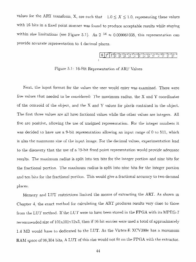
values for the ART transform, X, are such that -1.0 < X < 1.0, representing these values

with 16 bits in a fixed point manner was found to produce acceptable results while staying

within size limitations (see Figure 5.1). As2"14

0.000061035, this representation can

provide accurate representation to 4 decimal places.

s2" 2-' 2-- 2"3 2^ 2" -,-6 0-7 -,- T" ->-IC -r" T'2 1"" -,-H

Figure 5.1: 16-Bit Representation of ART Values

Next, the input format for the values the user would enter was examined. There were

five values that needed to be considered: The maximum radius, the X and Y coordinates

of the centroid of the object, and the X and Y values for pixels contained in the object.

The first three values are all have factional values while the other values are integers. All

five are positive, allowing the use of unsigned representation. For the integer numbers it

was decided to have use a 9-bit representation allowing an input range of 0 to 511, which

is also the maximum size of the input image. For the decimal values, experimentation lead

to the discovery that the use of a 19-bit fixed point representation would provide adequate

results. The maximum radius is split into ten bits for the integer portion and nine bits for

the fractional portion. The maximum radius is split into nine bits for the integer portion

and ten bits for the fractional portion. This would give a fractional accuracy to two decimal

places.

Memory and LUT restrictions limited the means of extracting the ART. As shown in

Chapter 4, the exact method for calculating the ART produces results very close to those

from the LUT method. If the LUT were to have been stored in the FPGA with its MPEG-7

recommended size of 101x101x12x3, then if 16-bit entries were used a total of approximately

1.4 MB would have to dedicated to the LUT. As the Virtex-E XCV300e has a maximum

RAM space of 98,304 bits, A LUT of this size would not fit on the FPGA with the extractor.

44

The solution to this problem was to take a different route, in particular the exact method

for determining the ART descriptor was implemented over the LUT method.

After the design had been implemented in VHDL, synthesis was performed. Through

synthesis and post-synthesis simulation, many of the characteristics of the design were found.

In particular, automatic report generated by synthesizing to the FPGA estimated that the

the maximum clock rate of the device would be approximately 35 MHz, but simulating

after routing and placing the design indicated that a lower clock rate was needed. Through

experimentation the maximum clock rate that was considered to provide proper functioning

of the device was 25 MHz.

The synthesis software also provided a means to estimate the power consumption of

the device. In ModelSim (tm), the simulation waveforms were captured to an output file.

These were then used as input to XPower(tm), a Xilinx provided software package. XPower

estimated that the device would use 5314 mW of power under normal operating conditions.

This and the other characteristics acquired through synthesis can be seen in in Table 5.1.

The design itself consists of five individual parts or stages. The first is the ART_STAT

module, which is responsible for the object statistics. Next is the COordinate Rotation

Digital Computer (CORDIC) Pipeline, used to convert the points of the object from Carte

sian to polar coordinates. After this, the radius is normalized by a divider. Following

normalization, the coefficients for the current point are extracted. Finally, the coefficients

are summed in the final stage. The next few sections will look at each of these stages in

detail.

45

Table 5.1: Characteristics of the Implemented Extractor

Logic Utilization

Number of Slice Flip Flops

Number of 4 input LUTs

791 out of 6,144

4,734 out of 6,144

Logical Units

Logic Distribution

Number of occupied Slices 3,070 out of 3,072

Number of Slices containing only related logic 3,042 out of 3,070

Number of Slices containing unrelated logic 28 out of 3,070

Total Number 4 input LUTs 5,306 out of 6,144

Number of bonded IOBs 92 out of 316

Number of Block RAMs 24 out of 32

Total equivalent gate count for design 472,398

Adders/Subtractors 5

Multipliers 4

Multiplexors 20

Comparators 6

Registers 47

Latches 14

Shift Registers 86

RAMs 2

ROMs 2

Design Specifics

Maximum clock rate 25 MHz

Clock Cycles per Point 68 (10 [Stage 1 + 16 [Divider] + [42 Stage 2])

Clock Cycles Between Points 36

Estimated Power Consumption (@ 25 MHz) 5314 mW

Pixels Processed per Second 69,444

46

[dis

enablei>-

Irese! l>-

I datain(18.TT>-

I datain(180)>-

rese!_l stals_rd_

d<17 0> q<!7 0>

d<170> q<170>

d<18 0> q<18 0>

H CX(17.0)>

I stats rd l>

I cv(17:0)>

I max rad(160)>

Figure 5.2: The ART_STAT Module

47

5.3 Implementation Details

5.3.1 The ART STAT Module

The statistic module, (see Figure 5.2), is responsible for the storage of the statistics of the

object on which ART is being performed. These statistics are the X and Y coordinates of

the centroid of the image (CX and CY respectively) and the maximum radius (MAXJRAD)

of the object. Statistics are stored once per object on the rising edge of the first three clock

cycles directly following a device reset and setting the RDJ3TATS-L pin to low. First, the

CX value is read in, followed by the CY value and the MAX RAD value, and stored (See

Figure 5.3). Each of these values are represented as 19-bit fixed point numbers as described

in the overview section.

RE/012

R = RESET^L

E = ENABLE_L

0 = CTLO (Capture CX)

1 = CTL1 (Capture CY)

2 = CTL2 (Capture MAX_RAD)

OX/000

11/000

10/100

1X/010

Figure 5.3: State Machine for STAT module

Figure 5.4 is a waveform from the behavioral simulation of the extractor for the

ART_STAT module. The signals CTLO, CTL1, and CTL2 are signals from this module's

control block that control the capturing registers. RD.STATS_L signals that the statistics

48

have been read and should not be read in again. ENABLEX triggers low if RD.STATSX

is low and the statistics have not been read in, thereby only allowing the statistics to be

loaded into the extractor once per reset.

'lestbench/ae/sl /r2p/p 1 /elk

'Iestbench/ae/s1 /r2p'pl /resetj

/tbstbench/ae/s1 / r2p/p 1 /xin

/lesibench/as/s1 / r2p/p1 /yin

/testberich/abJs 1 /r2p/p1 /quad

/testbench/ae/s1/r2p/pl/>tout

/lestbench/ae/s1/r2p/p1/yout

testbench/ae/s 1/r2p/p1 /tx

/ 1estbencrVae/s 1 / r2p/p1 /ty

/teslbench/ae/s1/r2p/p1/tx2

/teslbench/ae/s 1 /r2p/p 1 /ty2

/teslbencrVae/s1/r2p/p1/$1

/testbench/ae/sl/r2p/pl/s2

/lestberx:h/ae/si/r2p/pl/zero

/1estbench/ae's1/r2p/p1/xneg

/leslbench/ae/s1 It2p/p 1 /yneg

/Iestbench/ae/s1/r2p/p1/less

/testbench/ae/s1/r2p/p1/grealer

/lestbencrVae/s1/r2|Vpl/swap

/Iestbench/ae/s1/r2p/p1/guada

1HU110111U1HHUU1U

no 100

uuuumoimomooon UOUU0100"111100011101

00010010001000001110

ns

" ' '

""32C ns

" ' '

34C ns 36C

Enbty:!estbench Architecture struct Date Fn Jun 1 3 02 42 08 Eastern Daylight Time 2003 Row 1 Page 1

Figure 5.4: ART_STAT waveforms

5.3.2 Stage 1: The CORDIC Pipeline

This stage converts the input rectangular coordinates to polar coordinates. The pixel coor

dinates are read in simultaneously via the lower 18 bits of the input bus. Bits 17 to 9 are

the integer X coordinate and the lower 9 bits are the Y coordinate. These are then extended

with binary '0's to the 19-bit fixed-point representation previously described. Then they

are entered into the CORDIC process.

The CORDIC algorithm was originally developed to solve real-time navigational prob-

49

enable~r>-

I reset tV

I xin(19Q)>-

I Vlnl19 0)>-

I cy(19:0l>-

I cx(19.0)>-

{ aout(15:0)>

ml(19 0)>

| en next stage l)

I npr l>~

Figure 5.5: VHDL ART Stage 1 Module

lems [35]. It is a well known and widely studied iterative technique for mathematical func

tions such as multiplication, division, square root, sine, cosine, and inverse tangent [36]. It

is the trigonometric function capability of the CORDIC algorithm that is of interest.

Vector rotations can be used to compute all of the trigonometric functions. They can also

be used for polar to rectangular and rectangular to polar conversions, for vector magnitude.

and as a building block for transforms like the Discrete Fourier Transform (DFT) and the

Discrete Cosine Transform (DCT) [37]. The CORDIC algorithm is useful for digital signal

processing as it provides an iterative method that uses only shifts and adds to perform

vector rotations. The CORDIC algorithm is derived from the Givens rotation transform:

x = xcos<j) y sin0

y=y cos (j) + x sin (f>

This transform rotates a vector in a Cartesian plane by the angle </>. Rearranging these

equations gives the following:

x = cos cp [x -

y tan cp]

y'

= cos <j> [y + x tan cp]

50

By restricting the angle <f> to be composed of a series of successively smaller smaller rotations,

ai, such that j = tan~12~~\ the multiplication by the tangent term in the above equations

are reduced to simple shift operations. If, at each step, the coordinates are always rotated in

a positive or negative direction, then the increase in magnitude is considered to be constant.

The iterative versions of the above equations can be written as:

Xi+\ = Xi-

y{ di2"'

Vi+\ = Vi + Xi dt2"'

where:

ck= l

Each iteration of the system causes a gain in the magnitude of \/l +2~2%

. As the number

of iterations approaches infinity, the magnitude of this gain approaches 1.647. The exact

magnitude of this gain, K, would depend on the number of iterations such that:

K = H \/l +2- 2;

It is necessary to compensate for this gain by dividing the resulting values by K.

A third adder-subtractor is added to keep track of the elementary rotation angles at each

iteration. These angles are hardwired into each stage of the pipeline. This accumulator adds

a third equation:

zi+i=zt-di tan-1(2"1)

There are two modes associated with CORDIC, rotation and vectoring [35]. In rotation

mode the input vector is rotated by an angle that is given as an argument. In vectoring

mode, the input vector is rotated to the X-axis whilethe angle needed to make that rotation

is recorded in Zn . Since this thesis makes use of the vectoring mode of the CORDIC rotator

to perform rectangular to polar coordinate conversions, which uses the vectoring mode of

the CORDIC rotator, the rotation mode will not be explained here.

51

As noted above, the vectoring mode of the CORDIC rotator takes the input vector and

rotates it through the angle necessary to align the resulting vector with the x-axis. This

is done by sensing the sign of the y component and using it to determine the direction of

rotation. If the angle accumulator, Z, is initially set to zero then the result of the operation

will produce the rotation angle in Z and the scaled magnitude of the original vector in X.

The equations for the CORDIC rotation in this mode are [37]:

Xi+i =Xi-yi-di-

2~l

Vi+i = yi +Xi-di-

2~l

zi+i=

Zi-

di tan"1(2~2)

where:

, ( i if yi < odi= <

1 otherwise

The angles of rotation used by this algorithm are limited to be between = and | due to

the use of2

being used in the first iteration. If the composite rotation angles larger than

| an initial rotation must be made. Voider describes an initial rotation of 90 degrees which

would require the X and Y values to be switched. Another option is to perform an initial

rotation of n or 0. Performing the second choice gives the following equations:

x'

= d x

y =d-y

z if d = 1

z tt if d = 1

d

-1 ifx<0

+ 1 otherwise

This initial rotation does not add any gain to the system and assumes that the input angle

is represented in a modulo 27T form.

52

There are several ways to implement the CORDIC rotator as described in [37]. Of

interest to this thesis was Section 4.2 in [37], "On-Line CORDIC Processors". The CORDIC

iteration process is unrolled as described in [36]. Unrolling allows the shifts at each iteration

to be fixed, thereby eliminating shift registers and allowing wiring to be used instead. Also,

registers can be completely eliminated, leaving one large combinational circuit. In this

thesis, registers were added after every third stage to facilitate the pipelining of the design.

Finally, unrolling allows the angle accumulator values to be hardwired, reducing memory

storage requirements. In a non-unrolled CORDIC processor, the same hardware is used in

each stage yet different angle values are needed with every iteration of the processor. This

requires the implementation of a LUT to store and retrieve these values. Unrolling provides

each iteration with its own hardware, thereby eliminating the need for a LUT.

The specific design used was modified from [38]. The design consists of fifteen CORDIC

stages, a pre-processing unit, and a post-processing unit as can be seen in Figure 5.6. The

preprocessor modifies the data so that the point is in the first quadrant and the larger of

the values X and Y is placed in X. It makes note of the changes made and sends them to

the post-processor. The post-processor compensates for the system gain of the CORDIC

process and modifies the calculated angle so that it is placed in the proper quadrant.

I xinM9:0)>-

|yin(19:0)>-

I reset I)

xin<19 0> quad<2 0>

ym<19 0>

resetj yout<190;

r

xm<190> xout<19-0>

yin<19 0>

zm<17 0>

elk

resetj zout<17 0>

ain<17 0> aoul<15 0>

quad<2 0>

nn<19 0> roul<19-0>

I aoul(15:0l>

ut(19:0)>

Figure 5.6: The pre-processor (left), CORDIC pipeline, and post-processor (right)

53

This design was then modified to fit within the Xilinx FPGA. First, the pre-processor and

post-processors were modified to be single stage units instead of multiple stages. Also, in the

pre-processor, when it was acquired, was converting the sign of a value by just inverting the

sign bit. This was corrected such that 2's compliment was performed in order to change a

value's sign. Next, the CORDIC pipeline was modified from being fifteen individual stages

to five stages each of which contain three unrolled iterations of the CORDIC algorithm.

Finally, all of the signal paths were modified to handle the data sizes of this particular

design.

The module takes in two 19-bit fixed-point numbers and outputs the angle in a 16-bit

fixed-point number and the radius as a 20-bit fixed-point number. The method used to

compensate for the gain from the CORDIC algorithm gives a 0.0034% error.

Figure 5.7 shows waveforms for Stage 1 of the extractor.

Stage 1 of the ART extractor takes in the coordinates of the object's centroid that are

stored in the ARTJ3TAT module along with the X and Y coordinates of the current point.

10 clock cycles later the point's polar radius and angle are output.

5.3.3 Divider

The next step in the ART Extractor is to normalize the radius of the point relative to the

MAX_RAD value stored in the ART.STAT module. This custom designed divider consists

of four 2-to-l multiplexers, four delay registers, a comparator, a subtractor, and a 2-input

AND gate as can be seen in Figure 5.8.

The design is very straightforward. First, the radius is loaded into Register A and

MAX-RAD into register B. In the first clock cycles it determines if the input radius is

larger than the MAXJIAD value. If so, then the output of the divider is forced to be the

fixed point equivalent of 1.0. Otherwise, for the next 16 cycles, Register B is subtracted

from Register A. If Register A is larger than or equal to Register B, the result is stored

54

~

V) J3?- ~

-S ra -

tn ^ ^

n ! t!

Ifi ** CD OJ*-

O

-J C\J OJ

5 SB s ?W) (fl "fc ^ ,-

T~

H ti q)

2u --

Figure 5.7: Example Waveforms for Stage 1

55

Ife

!

t

ttl

11

( i

I

ffl

Figure 5.8: Block diagram of the Divider

56

in register A and a'1'

is placed in the current output bit. Otherwise, register A remains

unchanged and a'0'

is placed in the current output bit. Register B is shifted one bit to the

right and the process starts again. At the end of 16 clock cycles, the normalized radius is

in the output register of the divider.

Figure 5.9 shows the simulated waveforms for the divider. DONE_L signals the next

Stage 2 to read the QUOTIENT and to begin processing.

5.3.4 ART Stage 2

Stage 2 (see Figure 5.10) is where the extraction of the ART coefficients occurs. The

inputs for this module are the angle and the normalized radius of the current point. The

TEMP_BLOCK unit calculates the value of TEMP which is cos(N NORM.RAD). The

MULTJVI unit calculates COS_ANG which is (M * ANGLE)mod 2ix.

The REAL-BLOCK calculates the real values of the ART coefficients defined as TEMP*

cos(COSJiNG). It takes in the TEMP value and the COS.ANG value and in two stages,

first calculating the cosine value and then multiplying that value times the TEMP value.

The IMAGJ3LOCK calculates the imaginary values of the ART coefficients defined as

TEMP sin (COS^.NG). It does this in basically the same way as the REAL_BLOCK.

The sine and cosine units used in these blocks were custom designed using LUTs. The

LUT contained 12-bit values for first quarter wavelength. The rest of the waveform was

calculated from these values. The following methods were used:

LUT(n) n < 0.5

1 - LUT(n -

0.5) 0.5<n<1.0

0-LUT(n-l) 1.0<n<1.5

-1 +LUT{n-

1.5) 1.5<n<2.0

sin(n)= <

57

< .

Q<

CD

==

<

CD

< JJ

Xi

J_

J)J.

o-

c

f

Ju

J-

"D

X

X)

J.

o

< <

-

CD

<

CD

-

6

o

*-

X)

JJ

J.

X)

J-

J.

JJ

X)

J_

-L

X

3

v-

c

{Oj.

o

OJ

LL

CD

O

(J

~

O

J

<

< <

XI

J-

-~-

3

J-

JJ

XI

3

_c

jLL

O

J.

J.

O

IO

J-

o

<

uCD

<

o

oCD

<

<CD

OCD

<

oCD

CD

x>

3

j.

j.

s.

j_

j_

33

3

J.

3

O

J."-

O3

Zct

\n

3

3

j.

o

3

co

1

CD

u

O

CD CD

.

O

OCD CD

O

J_

3

O

-

X)

3

3

J-

X)

o3

J-

33

~C-c

Z

IOo

o

3o

3

X)oo->

<

<

O

O<

CD

U

<

=

Q CD

O

<

UCD

<

33

33

3

OO3

OOO

33

O

CD

3o

3

cc

Z

o

o

o

CD

=

O<

co

jj JJ

.o

CD

O<

CD

JJ

<

CD

O

s.

o

<

m

o

u

o<

CD

U3

3

CD

CD

O

o3

O3

O

5o

O

L Poo3

35o o

rvt

o

QCD CD m

o3

3

CM

O

o3

3

3

3

3

r-

CM CD

I 2 fio 5 5 5 5d ^ ^ r; r;

if) <> CO Q)

.- .- t- i- r-

T3

CD CD CD CD

5 5 E E

cj w to to to

? 2

Figure 5.9: Waveforms for the divider

58

Him MliOl)

-li. OUH15 0I>

^Su>

Figure 5.10: VHDL Stage 2

59

cos(n)= <

LUT(n) n < 0.5

-l + Lc7T(n-0.5) 0.5 < n< 1.0

0-LUT(n-l) 1.0<n<1.5

l-LUT(n-1.5) 1.5<n<2.0

Example waveforms for this block can be seen in Figure 5.11. In it, RIN and AIN are

the input angle and radius. NPR_L signals if another point can be added to the extractor.

EN_SUM enables the summation block. RE-OUT and IM_OUT are the real and imaginary

ART coefficients respectively.

5.3.5 The Summation Block

The summation block of the ART Extractor consists of two RAM modules, one adder,

one subtracter and several multiplexers. The first set of coefficients will become the initial

values in the RAM modules. Until the first set of coefficients are added, the values inside

the RAM blocks are unknown. Each consecutive set of coefficients will be added to, (in the

case of the real coefficients), or subtracted from, (in the case of the imaginary coefficients),

the values currently stored in the RAM modules. When the module is in a state such that

it can output the values of the coefficients, it will set the DONE signal to logical '1'. When

the RD_COEFS_L signal is set to logical'0'

while the DONE signal is high, the module will

output the current values it has stored, beginning with the first coefficient and outputting

another coefficient every clock cycle until all 36 coefficients are output.

34 bits are used for storage of the real coefficients and 33 bits are used for storage of

the imaginary coefficients due to the potential of the real coefficients to be larger. The

number of bits needed was determined by using MATLAB. In MATLAB, a 512 x 512 image

was created with every pixel being a part of the object. All of the coefficients above zero

were summed with their respective coefficients as were all the coefficients below zero. This

provided the absolute maximum and minimum values that the extractor may need to store.

60

1 1

1 : 1

$

i

-,

J

>-*

ss

=^

f

s

s

1

i

1

I

\

=1

PL

[I

II

Is

1

O

Oo

CO

o

XI

"

to

f>

*t

CD

CM

O

XI

<

CO

Oo

1 o

s

1

I

8

cm

"--

CD

f)

T

CD

CM

O

D

<

X)

o

cL

C

1OO

OO

,-

:

=

i

5

s

3

z*

=

a-

CD

CM

3

n

<

CD

r-

O

o

U

C

n

s

t

s

i

<

<

1O

Oo

OOo

o

<

<

1

S

9

O

O

O

OLL

i o

<J0

IT)

"3-

CD

OJ

O

o

o

CL

E

F

O

E

c\J m ntn ai nj

S

CD CO 0) CM

-5 "35 Ki I

ffi IS

Figure 5.11: Art Stage 2 Waveforms

61

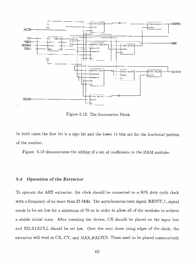
lx1MS0)>-

LH^

r

-

Ok waddi<5D> -

Cl5"0> rr.u'.i-. '-

><33> q<33-0>-

l<33-0> nu<33-0>-

-I zout(330

T_

s<32-0> q<32 0>-

-

Int.:32 0> nu<32-0>-

-

m232-0>

U32 0> ddt<32-ft. -

-I ZDutH3Z0)>

-

mi*i5tb ri

- lnJ<15Cr>

Figure 5.12: The Summation Block

In both cases the first bit is a sign bit and the lower 14 bits are for the fractional portion

of the number.

Figure 5.13 demonstrates the adding of a set of coefficients to the RAM modules.

5.4 Operation of the Extractor

To operate the ART extractor, the clock should be connected to a 50% duty cycle clock

with a frequency of no more than 25 MHz. The asynchronous reset signal, RESET_L, signal

needs to be set low for a minimum of 70 ns in order to allow all of the modules to achieve

a stable initial state. After resetting the device, CX should be placed on the input bus

and RD-STATS-L should be set low. Over the next three rising edges of the clock, the

extractor will read in CX, CY, and MAX-RADIUS. These need to be placed consecutively

62

< J L

u i isi

E

F

J :nnj<- CM CM

E E E E P

_i Ea E

E E ^ E

.- .-

CO CO

c 3 g g

E EI I 1

^ CD CD

CD CD -O

Figure 5.13: The Summation Block Waveforms

63

on the input bus. (Refer to Figure 5.14) Once the image statistics have been read in,

RDY_FOR_NXT_L will go low, signaling that the extractor is ready to accept a coordinate

point for input. The X and Y coordinates of the point should be placed on the input bus

and PTJ1DY_L should be set low. The extractor will then read in these coordinates and

begin to process them. The user will be able to add another coordinate every 36 clock cycles

after the last point was loaded into the descriptor.

Once all points have been entered into the extractor and it has finished all it's processing,

the DONE signal will go high. When this happens, the RD_COEFSX input should be

set low to make the extractor begin outputting the coefficients. The first coefficient will

be available one clock cycle after RD_COEFS_L is read with the next coefficient being

output on the consecutive clock cycles until all 36 coefficients have been output. (Refer to

Figure 5.15) A visual diagram of communication between the host computer and the FPGA

based extractor can been seen in Figure 5.16.

5.5 Results

The design was simulated on multiple levels. It was initially simulated at the behavioral

level. Once it was determined that the design functioned as desired, it was synthesized for

the Xilinx Virtex-E XCV3000e. After synthesis, the design was again re-simulated to verify

proper functioning. Finally, the design was mapped, routed and placed for the Xilinx chip

and the final simulation was run.

Table 5.2 shows the real part and the imaginary part of the coefficients, as calculated

by the FPGA via the simulations and how they compare to the exact values calculated

in MATLAB. In the table, the first column specifies the coefficient by its angular and

radial number. The second column lists the sum of each of the individual real coefficients

in VHDL while the third column lists the sum of the real coefficients as calculated in

64

u

L

J

E

F

Q

E

5 J

J

ai

<p q> a

Figure 5.14: The initial stages of Operation for the ART Extractor

65

L

Figure 5.15: Acquiring Coefficients from the ART Extractor

66

131

Computer RESETFPGA

READ OBJECT STATISTICS and CX

?

CY

MAX_RADIUS

READY FOR NEXT POINT

POINT READY and Point Coordinates

READY FOR NEXT POINT

POINT READY and Point Coordinates

?

READY FOR NEXT POINT

POINT READY and Point Coordinates

READY FOR NEXT POINT

DONE

READ COEFFICIENTS

COEFFICIENT(0,0)

COEFFICIENT^, 1)

COEFFICIENT(2,11)

Figure 5.16: HOST-FPGA Interaction

67

MATLAB. Column four lists the absolute difference between these two sets of values. The

fifth and sixth columns show the VHDL imaginary coefficients and the MATLAB imaginary

coefficients respectively. The seventh column presents the absolute differences between these

two values.

Table 5.3 shows the normalized coefficients for both the FPGA and the MATLAB code.

Once again, the first column specifies the coefficient by its angular and radial number. The

second and third columns respectively show the normalized coefficients for the FPGA and

MATLAB while the fourth column shows their absolute difference.

As can been seen in the tables, for this image the maximum difference between the

summations is 5.498538 and the maximum difference between the normalized coefficients is

0.000451. The maximum error for both the summations of the coefficients is less than 1.8%,

with the majority of the errors being less than 0.25%. For the imaginary summations the

maximum error for both is 34.08%, but this is an outlier with the majority of the of the

error is less than 0.45%.

These outliers occur with coefficients that have extremely small values, such as the

imaginary coefficients for n = 2, m = 9 in Table 5.2. The sum of the coefficient is relatively

close to zero when compared with the other coefficients and it is small enough that it is

close to the error of the extractor. This error is caused by the approximation of the sine

and cosine. While these outliers will happen again when the sum of the coefficients is small,

the numeric difference the outliers create in the final descriptor (and therefore the distance

between this descriptor and another descriptor) is small enough that it is of little concern

to the user.

These differences between the summations from the FPGA and MATLAB have little

effect on the normalized coefficients as can be seen in Table 5.3. The maximum differ

ence between the normalized coefficients as calculated by MATLAB and by the FPGA is

68

0.000451. The maximum percentage error is extremely low, being less than 0.8%.

To calculate how long a transform will take using the extractor, the number of pixels, i,

in the object must be determined. Then the following equation can be used to determine

the number of clock cycles needed:

ClockCycles(i) = 3 + (36 * (i + 1)) + 32

The coefficients for each point take 36 clock cycles to output. It takes 32 clock cycles to

initially fill the pipeline of the ART extractor and an additional 36 clock cycles to output

the sum of the coefficients for all of the points, (hence the addition of i to i). The addition

of 3 takes into account the initial three stages needed to add the images statistics.

Finally, the number of clock cycles is multiplied with the period of the clock to obtain

the minimum time required to extract the ART coefficients, assuming that input data is

ready when the extractor needs it and the extractor is instructed to immediately outputs

the coefficients when they are ready.

The worse-case scenario for the extractor is having a 512x512 image where every pixel

is turned"on"

In this case, the time required to process the pixels is:

NumberOfPixels = 512 512 = 262, 114

ClockCycles(2Q2, 114) = 3+ (36 * (262, 115)) + 32 = 9, 436, 175

ClockCycles 9,436,175,,

ErerutionTime = = - = 0.377447sexecution! ime

clockFrequency 25,000,000/^

This means that in the worse case scenario, the extractor can process approximately 2.6494

512x512 images per minute. This equates to approximately 694,440 pixels pixels per minute.

5.6 Parallelization of the Design

As the extractor outputs just the sum of the coefficients and as the coefficients for a given

point depend only on the coordinates of the specified point, the extractor is easilyparal-

69

Table 5.2: VHDL Computed Coefficients versus Exact Calculated Coefficients

n,m VHDL Real Exact Real \Difference\ VHDL Imaginary Exact Imaginary \Difference\

0,0 12192 12192 0 0 0 0

0,1 761.865000 761.931183 0.066183 534.054000 533.650000 0.404000

0,2 -4761.780000 -4759.096622 2.683378 4399.680000 4402.500000 2.820000

0,3 -1003.930000 -1003.086037 0.843963 938.285000 938.770000 0.485000

0,4 -96.619100 -98.363495 1.744395 -4000.880000 -4000.600000 0.280000

0,5 251.913000 252.663808 0.750808 697.015000 697.350000 0.335000

0,6 439.801000 440.427453 0.626453 2262.260000 2262.200000 0.060000

0,7 -974.429000 -974.485193 0.056193 438.428000 439.310000 0.882000

0,8 -1216.860000 -1217.203113 0.343113 -2024.330000 -2024.300000 0.030000

0,9 390.671000 390.208063 0.462937 -1261.950000 -1262.400000 0.450000

0,10 1545.090000 1544.789575 0.300425 454.835000 454.330000 0.505000

0,11 430.431000 430.408404 0.022596 662.472000 662.690000 0.218000

1,0 2153.200000 2147.701462 5.498538 0 0 0

1,1 1020.460000 1020.598773 0.138773 736.419000 734.780000 1.639000

1,2 301.894000 303.623387 1.729387 -1683.280000 -1686.100000 2.820000

1,3 -1262.490000 -1260.223217 2.266783 1561.770000 1561.700000 0.070000

1,4 436.800000 437.276434 0.476434 1082.230000 1083.600000 1.370000

1,5 -948.979000 -949.104711 0.125711 -828.414000 -828.050000 0.364000

1,6 -834.978000 -834.711917 0.266083 -350.287000 -351.570000 1.283000

1,7 1279.240000 1279.606733 0.366733 -282.081000 -282.960000 0.879000

1,8 438.885000 439.623348 0.738348 1142.340000 1141.800000 0.540000

1,9 -189.927000 -189.470075 0.456925 851.634000 851.500000 0.134000

1,10 -646.119000 -646.796048 0.677048 -247.412000 -247.810000 0.398000

1,11 -115.983000 -115.725800 0.257200 -589.464000 -589.740000 0.276000

2,0 -1692.320000 -1693.854911 1.534911 0 0 0

2,1 -1224.950000 -1225.583537 0.633537 -646.236000 -646.170000 0.066000

2,2 1970.650000 1969.841240 0.808760 -1867.370000 -1868.200000 0.830000

2,3 842.705000 842.640645 0.064355 -1508.410000 -1510.100000 1.690000

2,4 -804.440000 -803.726333 0.713667 1634.930000 1634.400000 0.530000

2,5 1022.890000 1024.089261 1.199261 830.164000 829.480000 0.684000

2,6 174.546000 174.600946 0.054946 -1776.190000 -1776.300000 0.110000

2,7 -551.909000 -551.781583 0.127417 326.792000 326.960000 0.168000

2,8 963.875000 963.640119 0.234881 1142.340000 1141.800000 0.540000

2,9 66.327900 66.844902 0.517002 -1.104740 -1.675800 0.571060

2,10 -464.228000 -463.082521 1.14548 84.808900 84.561000 0.247900

2,11 -162.239000 -161.980678 0.258322 92.203400 92.571000 0.367600

Maximums 5.498538 2.820000

70

Table 5.3: VHDL Computed Normalized Coefficients versus Exact Calculated Normalized

Coefficients

n, m VHDL Exact |Di//erence|

0,0 1 1 0.0

0,1 0.07631 0.07630 0.000015

0,2 0.53176 0.53175 0.000005

0,3 0.11271 0.11268 0.000023

0,4 0.32825 0.32823 0.000019

0,5 0.06079 0.06084 0.000047

0,6 0.18903 0.18903 0.000005

0,7 0.08764 0.08767 0.000034

0,8 0.19373 0.19374 0.000012

0,9 0.10835 0.10838 0.000024

0,10 0.13211 0.13207 0.000035

0,11 0.06480 0.06481 0.000014

1,0 0.17661 0.17616 0.000451

1,1 0.10322 0.10315 0.000069

1,2 0.14027 0.14052 0.000253

1,3 0.16472 0.16460 0.000121

1,4 0.09572 0.09584 0.000119

1,5 0.10332 0.10331 0.000012

1,6 0.07427 0.07429 0.000021

1,7 0.10745 0.10749 0.000045

1,8 0.03607 0.03614 0.000066

1,9 0.07157 0.07155 0.000019

1,10 0.05675 0.05681 0.000064

1,11 0.04928 0.04929 0.000018

2,0 0.13881 0.13893 0.000126

2,1 0.11360 0.11364 0.000043

2,2 0.22268 0.22268 0.000001

2,3 0.14172 0.14184 0.000118

2,4 0.14945 0.14939 0.000065

2,5 0.10805 0.10809 0.000041

2,6 0.14639 0.14640 0,000009

2,7 0.05261 0.05261 0.000002

2,8 0.12259 0.12255 0.000046

2,9 0.00544 0.00548 0.000043

2,10 0.03871 0.03861 0.000096

2,11 0.01531 0.01530 0.000003

Maximum 0.000451

71

lelizable.

Assuming that the user has N FPGA extractors, parallelization can be achieved in the

following manner. First, the image must be read in by the computer and analyzed as in

the non-parallel method with the object points being placed into a list. Next the image

statistics need to be loaded into each FPGA. Along with this step, the computer needs to

divide the image points into N lists that have as equal a length as possible. The points

do not need to be divided in any particular order and can be randomly assigned to any of

the N lists. Each list shall be assigned to an individual FPGA which can process the list

as if it were all the points of the object. When each list is finished processing, the sums

from each FPGA need to be read and these need to be summed in order to get the total of

the coefficients for the object. Depending on how the user sets up the input busses for the

extractors, it is possible to achieve a near N speedup. It should be noted that full image is

still restricted to a maximum size of 512 x 512.

72

Chapter 6

CONCLUSION

6.1 Closing Remarks

The primary contribution of this thesis is an FPGA-based solution for the hardware im

plementation of the ART shape descriptor. It has shown that this is feasible and that the

proposed design is capable of processing approximately 69,444 pixels a second. This design

makes use of both the CORDIC algorithm and several custom modules in order to fit on a

Xilinx Virtex-E XCV300e.

The design has the potential for even higher speedups should certain problems be over

come. The first one is the restricting size of the FPGA used. Increasing the size of the

FPGA would allow for more efficient pipelining of the design. Once this is achieved, the

divider becomes the primary bottleneck of the system. A new design for this divider needs

to be implemented in such a way as to be able to keep up with the pipelined stages of the

multipliers that were used.

Even without these improvements, the proposed design has uses in today's imaging

world. One of the possible uses for this extractor would be its integration into an image

database retrieval system. The use of the extractor could alleviate some of the processing

requirements from the CPU of the computer hosting databases. Image retrieval systems,

such as the ones presented in references [4] , [5] or other databases that make use ofMPEG-7

shape metadata could be modified to make use of such a device.

Along with the proposed hardware design, the MPEG-7 shape descriptors were explored

for shape based retrieval from databases. Results showed that the majority of the retrievals

73

made using the MPEG-7 shape descriptors returned visually acceptable results.

Finally, this thesis briefly explored the potential of utilizing the ART descriptor for

optical character recognition. It demonstrated that while the ART has potential for OCR,

there is still research to be performed in this area.

This work will conclude with some possible areas for future research.

6.2 Areas for Future Research

There are several possibilities for future work:

The implementation and optimization of the ART extractor on a larger FPGA. This

would allow for some of the improvements mentioned above. A larger FPGA might

even allow for the implementation of the LUT method of calculating the ART descrip

tor.

The implementation of the CSS algorithm on an FPGA. While the main theory is

the same as presented in this thesis, the implementation of the CSS descriptor in an

FPGA-based hardware environment presents its own unique challenges that need to

be addressed.

The implementation of the matching algorithm for the CSS descriptors in hardware.

The matching algorithm as described in the last few paragraphs of Section 3.2. While

a relatively straightforward algorithm, it would be of interest to implement this in

hardware for a reduction in execution time. Also, the possibility of parallelizing this

algorithm should be explored.

The implementation of a database that makes use of MPEG-7 shape descriptors.

Building such a database could serve as a testbed for future research. The database

could be further expanded to include other MPEG-7 descriptors as needed.

74

The interfacing of the ART extractor with a database of images and making use of it

to speed up metadata extraction. If the database mentioned is built, the use of the

extractor presented in this thesis, could be utilized.

Designing a system that could make use of the parallelizable nature of the ART

algorithm. As explained in Section 5.6, it is possible to have several of the presented

extractors process different segments of the same image in parallel. It would be of

interest to explore this further and modify the extractor such that the segments that

it can process are limited to a 512x512 size, yet the size of the image as a whole is

not.

Further explore OCR using the ART. This thesis demonstrated that it is possible to

use the ART for OCR. Expanding on this work could lead to a reliable OCR system

based upon the ART descriptor.

It would also be of interest to explore how one can combine the CSS and ART descriptors

in order to locate one particular object.

75

Appendix A

MATLAB QUERY RESULTS

Figure A.l: Human Matchings for kkl83 (No Particular Order)

t^T ^X xl f '^ ^X f y'

\> ( M ca (> l \t-

s r \r

<-^ 's r <-, ro

kklBe kklOO kklOl kk!75 kkl30 kkiTns

\ A T A\ C(

UCP T- ^ ^r "'.Vkk651 kkl02 kklB9 Jck99 ^553

r V -A /\ A /-v

vf \ r \ ? x r sp

A-T N f-*(A kk304

kkl56kkl034

kk310 kk807

Figure A.2: Human Matchings for kkl88 (No Particular Order)

76

kk458 kk456kk452 kk455 kk724

f r

aV>'

kk36 kk449 kk9 kk462

kk6 kk460 kk564 kk454

1 J C

*=>

kk327 kk453 kk328

Figure A.3: Human Matchings for kk458 (No Particular Order)

77

n

<A

Figure A.4: Retrieval results from kkl83 using CSS

Oueiy Image

L,

S j

'

u

i v

l\

A1>

03589

y

c.

Figure A.5: Retrieval results for kkl88 using CSS

Ar>

0 241799 0 254192 0.313673

A iv />AA/

!A-'

'i 1

0.317328 0.324312 0 326907

A A: P

A

Figure A.6: Retrieval results for kk458 using CSS

78

<z.

A

0220129

fi

Figure A.7: Retrieval results for kkl83 using LUT based ART without filling

Query image

X0.181929

A,i

A0.1WOB3

X

A0 164905

S r

Figure A.8: Retrieval results for kkl88 using LUT based ART without filling

lr

0258555

A |

A7

\J

Figure A.9: Retrieval results for kk458 using LUT based ART without filling

79

JJ

..

'a'

A U

Figure A.10: Retrieval results for kkl83 using the exact ART without filling

rYi

0.349376 0.41OS19 0 42493

r-0 t-y A

A AV A A A

ta

0 427966 0 431127 0 43168

A.{

1'-

A

/ t

S r

Figure A.ll: Retrieval results for kkl88 using the exact ART without filling

0 325363

AJr

A/\l 1 A

AA.

Figure A.12: Retrieval results for kk458 using the exact ARTwithout filling

80

A

0 368752

I i

Figure A. 13: Retrieval results for kkl83 using LUT based ART with filling

rA

V

A-v

/ L

Xi0317321

<yXi~

031M1-1 o.3W7ae

n

Figure A. 14: Retrieval results for kkl88 using the LUT based ART with filling

X

0 357743

A

0 445283

u0 46A72

A

Figure A.15: Retrieval results for kk458 using the LUT based ART with filling

81

A

A;

Figure A. 16: Retrieval results for kkl83 using the exact ARt with filling

Query Image

'"Ar-i A

f u

0 0757667 0 0941867

xuA-

/ v_' L

\ c\ r\ri AO

0 101262 0 101754

^1~v"

rX i-A

\ T

Figure A. 17: Retrieval results for kkl88 using the exact ARt with filling

X0 127645

A

X

Figure A.18: Retrieval results for kk458 using the exactARt with filling

82

Appendix B

CHARACTER MATCHING RESULTS

(j c C

XD

./

A

Figure B.l: Examples of Handwritten Characters in the Database

83

aA aAaAaA

BBb

cCDdd

BBBbbbbccccCCCCCC

DdddDDDddeeE

eeEEEEEJC/P FFFFffggG

ggGCjMHhhhh i

Figure B.2: Examples of Typeset Characters in the Database

84

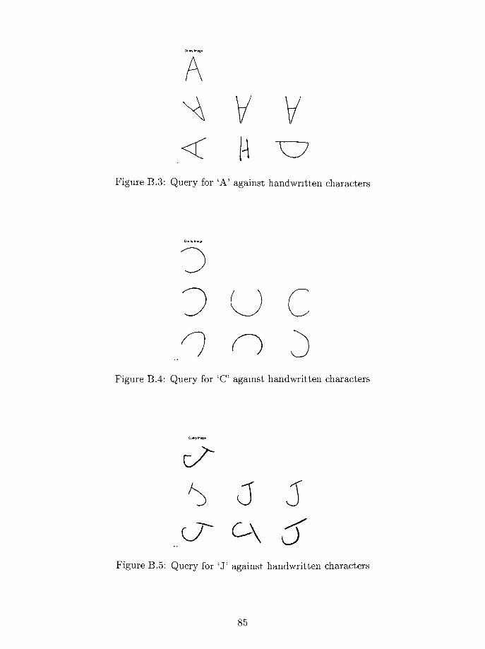
Figure B.3: Query for'A'

against handwritten characters

Figure B.4: Query for'C'

against handwritten characters

cA

^ J J

Figure B.5: Query for'J'

against handwritten characters

85

A A

AAAFigure B.6: Query for

'A'

against handwritten and typeset characters

cFigure B.7: Query for 'C against handwritten and typeset characters

cA

^ J J

cA F F

Figure B.8: Query for'J'

against handwritten and typeset characters

86

AAA

A A a

Figure B.9: Query for'A'

against typeset characters

C C G

c c cFigure B.10: Query for 'C against typeset characters

cA

F F F

F L LFigure B.ll: Query for

'J'

against typeset characters

87

Appendix C

CD CONTENTS

The following items can be found on the included CD:

MATLAB source code

C++ source code

VHDL source code

Shape contour database

Character and Typeset database

BIBLIOGRAPHY

[1] J. R. Smith and A. B. Benitez. Content Organization. In B.S. Manjunath, P. Salembier,

and T. Sikora, editors, Introduction to MPEG-7, pages 153-161. John Wiley and Sons,

LTD, 2002.

[2] F. Alaya Cheikh A. Quddus and M. Gabbouj. Wavelet-based multi-level object retrieval

in contour images. Technical report, Tampere University of Technology (TUT), 1999.

[3] S-F. Chang, T. Sikora, and A. Puri. Overview of the MPEG-7 Standard. IEEE Trans

actions on Circuits and Systems for Video Technology, ll(6):688-695, June 2001.

[4] M. Flickner, et. al. Query by image and video content: The QBIC system. IEEE

Computer, 28(9):23-32, Sept 1995.

[5] S-F Chang, et. al. Columbias VoD and Multimedia Research Testbed With Heteroge

neous Network Support. Journal on Multimedia Tools and Applications, Special Issue

on Video on Demand, 1997.

[6] Dr F Mokhtarian. Shape Queries Using Image Databases.

http://www.ee.surrey.ac.uk/Research/VSSP/imagedb/demo.html.

[7] B. Giinsel and A. Tekalp. Shape Similarity Matching for Query-by-Example, 1998.

[8] S. Fan. Shape Representation and Retrieval Using Distance Histograms. Technical

report, University of Alberta, 2001.

89

[9] P. W. H. Kwan, et. al. TAST Trademark Application Assistant. In In Proceedings

2002 IEEE International Conference on Image Processing, volume 1, pages 884-887,

2002.

[10] B. S. Manjunath, P. Salembier, and T. Sikora, editors. Introduction to MPEG-7:

Multimedia Content Description Interface. John Wiley & Sons Ltd., 2002.

[11] M. Bober. MPEG-7 Visual Shape Descriptors. IEEE Transactions on Circuits and

Systems for Video Technology, 11(6):716-719, June 2001.

[12] M.K. Hu. Visual Pattern Recognition by Moment Invarients. IRE Transactions on

Information Theory, IT-8:179-187, 1962.

[13] A. Sajjanhar, and G. Lu. A grid based shape indexing and retrieval methoed. Special

Issue of Australian Computer Journal on Multimedia Storage and Archiving Systems,

29(4):131-140, November 1997.

[14] E. Arkin, L.P. Chew, D.P. Huttenlocher, K. Kedem, and J. Mitchell. An efficiently

computable metric for comparing polygonal shapes. IEEE Transactions on Pattern

Analysis and Machine Intelligence, 13(3):209-215, 1991.

[15] C.T. Zahn and R.Z. Roskies. Fourier descriptors for plane closed curves. IEEE Trans

actions on Computers, C-21(3):269-239, 1972.

[16] K.L. Tan, B.C. Ooi and L.F. Thiang. Retrieving similar shapes effectively and effi

ciently. In B.S. Manjunath, P. Salembier, and T. Sikora, editors, Multimedia Tools and

Applications, volume 19, pages 111-134. Kluwer Academic Publishers, February 2003.

90

[17] R. C. Gonzalez and R. E. Woods. Digital Image Processing. Addison-WesleyPublishing-

Company, Inc., 1992.

[18] M. J. T. Smith and A. Docef. A Study Guide for Digital Image Processing. Scientific

Publishers, 1997.

[19] W-Y. Kim, Y-S Kim, and Y-S Kim. A new region-based shape descriptor:

The ART (Angular Radial Transform) Descriptor. ISO/IEC JTC1/SC29/WG11

MPEG99/M5472, December 1999.

[20] ISO/IEC JTC 1/SC 29/WG11/N4360. Information Technology Multimedia Content

Description Interface Part 8: Extraction and use ofMPEG-7 Descriptions, July 2001.

[21] E. R. Dougherty, editor. Fundementals of Electronic Image Processing. SPIE/IEEE

Series on Imaging Science & Engineering. SPIE - The International Society for Optical

Engineering & IEEE Press, 1996.

[22] MPEG-7 experimentation Model (XM) Software. Available from:

http://www.lis.e-technik.tu-muenchen.de/research/bv/topics/mmdb/e_mpeg7.html.

[23] C. K. Pokorny and C. F Gerald. Computer Graphics: The Principles Behind the Art

and Science. Franklin, Beedle, & Associates, 1989.

[24] E. Persoon and K.-S. Fu. Shape Discrimination Using Fourier Descriptors. IEEE

Transactions on Systems, Man, and Cybernetics, pages 170-179, March 1977.

[25] S. K. Bahl. A Hardware Efficient Architecture for Fast Fourier Transform. In Proceed

ings GSPx and International Signal Processing Conference, 2003.

[26] CYGWIN. Available from: http://www.cygwin.com.

91

[27] Libtiff Tagged Image File Format c library. Available from: http://www.libtiff.org.

[28] Independent JPEG Group c library. Available from: http://www.ijg.org.

[29] R. D. Wittig and P. Chow. Onechip: An fpga processor with reconfigurable logic.

In In Proceedings of the IEEE Symposium on FPGAs for Custom Compute Machines

(FCCM96), 1996.

[30] S. Brown and Z. Vranesic. Fundamentals of Digital Logic withe VHDL Design.

McGraw-Hill, 2000.

[31] J. L. Hennessy. Computer Architecture A Quantitative Approach Second Edition.

Morgan Kaufmann Publishers, Inc., 1996.

[32] T.C. Waugh. Field Programmable Gate Array Key to Reconfigurable Array Outper

forming Supercomputers. In In Proceedings of the IEEE Custom Intergrated Circuits

Conference, 1991.

[33] D. Van den Bout et al. Anyboard: An FPGA-Based Reconfigurable System. IEEE

Design and Test of Computers, pages 21-30, Sept 1992.

[34] P. M. Athanas and H. F. Silverman. Processor Reconfiguration Through Instruction-

Set Metamorphosis. Computer, pages 11-18, March 1993.

[35] J.E. Voider. The CORDIC Trigonometric Computing Technique. IRE Transactions

on Electronic Computers, pages 330-334, Sept 1959.

S. Wang and V. Piuri. A Unified View of CORDIC Processor Design. In E. E. Swartz-

lander, editor, Application Specific Processors, pages 121-160. Kluwer Academic Press,

November 1996.

92

[37] R. Andraka. A survey of CORDIC algorithms for FPGA based computers. Technical

report, Andraka Consulting Group, Inc, 1998.

R. Herveille. OpenCores.org Project: CORDIC core. Technical report,Open-

Cores.org, 2001.

93

''

:<:

BretWozRochester institute of Technology

Department of Computer Engineering

/

m

+

OkOj

tyPEG-1 ^

O

O

8?