MITSUBISHI ELECTRIC RESEARCH LABORATORIEShttp://www.merl.com

An Extended Luenberger Observer for HVAC Applicationusing FMI

Bortoff, S.A.; Laughman, C.R.

TR2018-205 March 15, 2019

AbstractIn this paper we show how a Functional Mockup Unit (FMU) may be used for the realizationof an Extended Luenberger Observer (ELO), which may be considered the deterministic ver-sion of an Extended Kalman Filter (EKF). The ELO has advantages over an EKF in somesituations, such as lower computational burden and improved convergence. Nonlinear ob-servers, such as those that make use of changes of coordinates to linearize, or approximatelylinearize the estimate error, are continuoustime dynamical systems that use so-called outputinjection to modify the dynamics of a model. Output injection provides a similar feedbackeffect as the correction step of an EKF. However, nonlinear output injection is a slightly FMUdifferent use case because the ELO is a continuous time object. It is realized by feedbackaround a modelsharing type of continuous time FMU, in contrast with the algorithmic re-alization of a discrete-time EKF, which uses the co-simulation form of FMU. We illustratethe design and realization of an ELO for a building HVAC example, in which we estimateunmeasured heat flows and unmeasured boundary conditions for use in a building “digitaltwin.” We also make some remarks about model reduction and the challenges in realizing aconventional EKF for these types of models.

International Modelica Conference

This work may not be copied or reproduced in whole or in part for any commercial purpose. Permission to copy inwhole or in part without payment of fee is granted for nonprofit educational and research purposes provided that allsuch whole or partial copies include the following: a notice that such copying is by permission of Mitsubishi ElectricResearch Laboratories, Inc.; an acknowledgment of the authors and individual contributions to the work; and allapplicable portions of the copyright notice. Copying, reproduction, or republishing for any other purpose shall requirea license with payment of fee to Mitsubishi Electric Research Laboratories, Inc. All rights reserved.

Copyright c© Mitsubishi Electric Research Laboratories, Inc., 2019201 Broadway, Cambridge, Massachusetts 02139

An Extended Luenberger Observer for HVAC Applicationusing FMI

Scott A. Bortoff1 Christopher R. Laughman1

1Mitsubishi Electric Research Laboratories, Cambridge, MA, USA, {bortoff, laughman}@merl.com

AbstractIn this paper we show how a Functional Mockup Unit(FMU) may be used for the realization of an ExtendedLuenberger Observer (ELO), which may be consideredthe deterministic version of an Extended Kalman Filter(EKF). The ELO has advantages over an EKF in somesituations, such as lower computational burden and im-proved convergence. Nonlinear observers, such as thosethat make use of changes of coordinates to linearize, orapproximately linearize the estimate error, are continuous-time dynamical systems that use so-called output injectionto modify the dynamics of a model. Output injection pro-vides a similar feedback effect as the correction step ofan EKF. However, nonlinear output injection is a slightlyFMU different use case because the ELO is a continuoustime object. It is realized by feedback around a model-sharing type of continuous time FMU, in contrast with thealgorithmic realization of a discrete-time EKF, which usesthe co-simulation form of FMU. We illustrate the designand realization of an ELO for a building HVAC example,in which we estimate unmeasured heat flows and unmea-sured boundary conditions for use in a building “digitaltwin.” We also make some remarks about model reduc-tion and the challenges in realizing a conventional EKFfor these types of models.Keywords: Estimation, Buildings, HVAC, FMI, FMU

1 IntroductionState estimation is one of the important use cases for theFunctional Mockup Interface (FMI). For example, statesof a nonlinear continuous-time model can be estimatedfrom discrete-time measurements of the input and outputof a plant using a continuous-discrete Extended KalmanFilter (EKF), realized using the co-simulation form of aFunctional Mockup Unit (FMU) of the plant (Brembecket al., 2014, 2011). Fundamentally, the EKF, and its vari-ous extensions estimate the state in a two-step process. Inthe prediction step, the EKF computes the predicted stateestimate using a discretized plant model. Then in the cor-rection step, the covariance and gain are computed as afunction of the predicted state estimate, and the predictedstate estimate state is corrected. The discrete-time pre-diction model is then initialized using the corrected state,and the process is repeated. Importantly, the two steps arecoupled in a causal manner: The prediction step at time

(k + 1) depends only upon the correction step at time k,and the correction step at time k depends only on the pre-diction step at time k. This fact allows an FMU to be usedin an algorithm to estimate the state in the prediction step,since it can be initialized using the corrected state estimatefrom the previous correction step.

An observer is an alternative technology for estimationof the plant states and parameters. An observer is a de-terministic, continuous-time dynamical system that takesas input the measured input and measured output of theplant, and produces as its output an estimate of the stateof the plant. It is similar to the Kalman filter, but based ondeterministic assumptions and mathematics. Fundamen-tally, the concept of output injection is used to stabilizethe observer error dynamics, which govern the differencebetween the estimated state and the plant state. OutputInjection means that a signal is injected (added) to thederivative of the observer state vector as stabilizing feed-back. Because of this, it is the continuous-time dynamicsof the plant with output injection that needs to be sim-ulated. There are not separate prediction and correctionsteps.

In this paper we show how an instantiation of a model-exchange type of FMU can be used with the Dymola toolto realize output injection, enabling design and implemen-tation of linear and nonlinear state observers and specifi-cally the Extended Luenberger Observer (ELO). Our spe-cific interest is to estimate unmeasured performance vari-ables of a building and HVAC system as a part of abuilding “digital twin.” Toward this end we have con-sidered several alternative methods to estimate the per-formance variables, including various flavors of the EKF.However, these may prove too computationally burden-some for our application because the number of states canbe large (hundreds), the number of measurements can belarge (tens to hundreds), and the EKF can be computa-tionally challenging because of the covariance update, al-though there are many techniques such as model reductionand square root filtering that are available to improve itscomputational efficiency. More importantly, an EKF canfail to converge, or in some cases, cause the model to failat run time, at least for our building HVAC applications.Convergence failures are caused by some of the character-istics of the model that we consider in this paper, whichare not unusual for this field of application. The modelis stiff (with time constants ranging from milliseconds to

several weeks — eight orders of magnitude), and is nu-merically ill-conditioned (with states varying 8-9 ordersof magnitude because of the choice of units). Thus the Ja-cobian may not accurately predict the state over the fixedand usually large EKF sample time, causing it to diverge.Moreover, the model itself contains state constraints, suchas a non-negative limit on mass concentrations, which canbe violated at run time because of the EKF correction step,causing a run-time error.

On the other hand, the ELO is relatively simple andlight-weight computationally. In its simplest form, it usesa constant feedback gain matrix that is computed at de-sign time from the steady-state solution of a Ricatti equa-tion, and therefore avoids the real-time covariance updateand computation of the system Jacobian that is necessaryfor the EKF. Further, it may offer improved stability andperformance advantages over the EKF (and similar filters)for certain applications because it makes use of implicitvariable-step solvers for the continuous-time model.

This paper is organized as follows. In Section 2, we re-view the basics of the Extended Luenberger Observer. InSection 3, we construct an ELO for a case-study buildingand HVAC system and show some simulation results. Weshow how the FMU is used to allow for the output injec-tion. Finally in Section 4 we conclude by making someobservations on potential improvements of FMI to betterenable realization of estimators of different types.

2 BackgroundFollowing (Zeitz, 1987), consider the nonlinear system

x = f (x,u,d) (1a)y = h(x) (1b)z = g(x) (1c)

where x ∈ Rn is the state, u ∈ Rm is the control input, as-sumed measured, d ∈ Rq is a disturbance measurement,assumed measured, y ∈ Rr is the measured output, andz ∈ Rp is the performance output, assumed unmeasured.Our objective is to estimate the performance output z. TheExtended Luenberger Observer is the system

˙x = f (x,u,d)+K(y− y) (2a)y = h(x) (2b)z = g(x) (2c)

where x ∈ Rn is the state estimate, z ∈ Rq is the perfor-mance output estimate, and K is the observer gain. Sys-tem (2) is a copy of the original system, with the vectorK(y− y), which is called output injection, added to thestate equations.

The state estimate error x = x− x is then governed bythe system

˙x = f (x,u,d)− f (x,u,d)−K(y− y) (3a)y = h(x)−h(x) (3b)z = g(x)−g(x). (3c)

We linearize (3) about an equilibrium x in a neighborhoodof x, defining

F =∂ f∂x|x=x , H =

∂h∂x|x=x , and G =

∂g∂x|x=x , (4)

so that the linearized error dynamics, neglecting higher-order terms, are

˙x = (F−KH)x (5a)y = Hx (5b)z = Gx (5c)

There exists an observer gain K to make the origin of (5a)locally exponentially stable if the pair (F,H) is detectable.

There are many methods for the design of the observergain K e.g. (Luenberger, 1971; Chen, 1984; Friedland,1986). In fact, more generally we can consider nonlin-ear changes of state coordinates z = Φ(x,u,d), nonlinearchanges of the output coordinates ξ = Γ(y), and nonlin-ear output injection K(y) as in (Krener and Isidori, 1983;Krenner and Respondek, 1985; Hou and Pugh, 1999). Re-search on methods for computing these remains an ac-tive area of research e,g, (Boutat et al., 2009; Tami et al.,2013). Here we will simply linearize the system (1) aboutan equilibrium and compute the gain K that minimizes thequadratic cost

J = min∫

∞

0zT Qz+ yT Rydτ (6)

by solving the steady-state Algebraic Riccati Equation

0 = AP+PAT −PHT R−1HT P+ΦT QΦ, (7)

from which the observer gain is K = (R−1HP)T .

3 Building “Digital Twin” Case StudyIn this section we design an ELO to estimate unmeasuredperformance outputs in a commercial building HVAC sys-tem. The primary purpose of the observer is to estimateheat flows through the walls, ceiling and floor, and alsoto estimate the unmeasured heat loads, denoted q, in theoccupied space. These estimates can be used to better un-derstand building performance and improve human com-fort and energy efficiency.

The building, diagrammed in Figure 1, is the top floorof a medium-sized commercial office building, with openfloor plan for office work. We model the floor as a singleroom with four outside walls, a floor and a ceiling. Abovethe ceiling is a small plenum space that separates the ceil-ing from the roof. The walls are made up of between oneand four layers of building materials. Windows are onthe South and West facing facades. The air conditioningsystem is a chilled water plant, with fan coils for cool-ing. Outside air ventilation is provided by a constant speedventilation fan, and the outside air passes through an En-ergy Recovery Ventilation Unit (ERV) for pre-cooling in

Plaster BoardAir

Rockwool

Carpet Tile

Air

Concrete Slab

Ceiling Material

Concrete

RoomMixed

Air

SouthFacing

Window

ALC

OutsideAir

South andWest Wall(Outside)

North and East

Wall (Indoor) Constant Indoor Temperature

Constant Indoor

TemperatureScaled-UpRAC

OutsideAir

Insulation

Plenum

Roof

Blinds

Outside Wall x 4

Floor

Outside Wall Orfice

OrficeOutsideAir

PIControl

TMY3Weather(Tokyo)

Ventilation Air Fan

Figure 1. Building with plenum.

the summer season, but is otherwise not treated. For pur-poses of design, we assume there are three measurementsavailable on a one minute sampling interval: The roomtemperature Tr, the plenum temperature Tp, and the returnwater temperature Tw. We also assume that the weathervariables are measured hourly. These include the outsideair temperature, humidity, wind speed, direct and indirectsolar radiation in visible and infra red radiation, cloud con-ditions, and the atmospheric pressure. The room tempera-ture Tr is compared to a reference set-point, and the erroris fed back through Proportional-Integral (PI) feedback toactuate the valve in the fan coil.

The system is modeled using the Modelica buildingslibrary (Wetter et al., 2014) as two rooms: one represent-ing the working space, and the second representing theplenum, as shown in Figure 2. The outside walls have fourlayers, and the windows are double-paned glass. Orficesare put between the plenum and room to represent airflowbetween them, although its velocity is very close to zeronominally. A cooling coil is connected to a variable speedchilled water pump to provide variable capacity cooling.An Energy Recovery Ventilator (ERV) is included to pre-cool the outside ventilation air, which is provided at a fixedrate. All of the model components are taken from theModelica buildings library. Typical Meteorological Year(TMY) weather for Tokyo is used in all simulations. Thecomplete model has 85 states, three measured outputs, oneinput (the water pump speed), and eleven disturbance in-puts corresponding to the eleven weather variables used inthe building library. A PID controller from the ModelicaStandard Library is added to the model later for feedbackto regulate the room temperature to a desired set-point.

We now step through the design and implementationsteps, beginning with model augmentation, which is donein order to estimate unmeasured model inputs, then modellinearization, order reduction, feedback gain design, andFMU realization.

3.1 Model AugmentationAfter constructing the nominal model, it must be modifiedfor use as an estimator. Normally the heat load q is consid-ered an input to the model. (Actually, there are three dif-

ferent types of heat load: Radiative, Sensible and Latent.Here we assume all of the heat load is sensible.) However,in order to estimate q from the available measured outputs,we augment the model to include q as a state. We assumethat the heat load is constant, and then add the equation

q = 0 (8)

to the Modelica model. This is done by adding an inte-grator to the model as the heat load, with its input set tozero. This will allow us to estimate the heat load with zerosteady-state error if it is constant, and a small tracking er-ror if it is time-varying.

Mathematically, the building and HVAC model is

x = f (x,u,d,q) (9a)q = 0 (9b)y = h(x) (9c)z = g(x) (9d)

where z is the heat flow through the surfaces of interest(floor, walls, ceiling, and window), y is the three measure-ments, x is the 85-dimensional state vector, d representsthe measured weather inputs into the model, and u is thewater valve control input. The model used for estimatordesign does not include the PI feedback controller, whichis added later for simulations.

3.2 LinearizationWe then simulate model for approximately one millionseconds (about 1 week). This is necessary because theslowest observable mode in the model has a time constantof approximately eight hours, which comes from the con-crete building materials in the walls. For the linearization,we zero the radiative effects of the weather, and assumethe outdoor temperature and humidity are constants repre-senting typical weather in the summer. This is not ideal,since the radiative effects are dominant. However, it is ef-fective for this particular application. The linearization is

Weather

Heat Loads (3)

Ventilation

Temperature Controller

Water Based Cooling

PlenumRoom

Figure 2. Modelica model.

represented as

x = Ax+Bu (10a)y =Cx (10b)

3.3 Observer Gain DesignWe design the observer gain K ∈ R86×3 as outlined in theprevious section, with a penalty Q ∈ R86×68 on the esti-mated states, and R ∈ R3×3 penalizing the measurements.For simplicity, these are set to be diagonal matrices. How-ever, we find that a solution to the Riccati equation (7) forthe linearized model and any such values of Q and R doesnot exist! We must analyze the linearized model (10), andthen modify and reduce it in order to properly design thefeedback gain K.

Computing the spectrum of A, we find a total of threestates have eigenvalues at exactly zero, one state has aneigenvalue at almost zero, but corresponding to a timeconstant of several months, and the remainder have realnegative parts with time constants ranging from 12ms to7hours, as expected. (It may surprise the reader to seesuch fast modes in a model of an HVAC system. Theseare due to heat flow in the metal heat exchanger.) One ofthe three zero eigenvalues corresponds to the integrator,which can be verified by computing the left eigenvaluesof A and showing that the integrator state corresponds ex-actly with the corresponding left eigenvector. (This meansthat the integrator state is affected by none of the otherstates, but it does affect other states, and is, in fact, ob-servable.) The other two states with exactly zero eigen-value correspond to “physical” states that are introducedinto the orfice equations in the model, which can be seenby inspecting the following code taken from the Modelicabuildings library.

Real mExc(quantity="Mass", final unit="kg")"Air mass exchanged (for purpose of

error control only)";initial equationmExc=0;

equationif forceErrorControlOnFlow thender(mExc) = port_a.m_flow;

elseder(mExc) = 0;

end if;

We see that the state mExc is introduced for er-ror control, and has its derivative set to zero ifforceErrorControlOnFlow=false. This statehas no effect on a simulation, but it is included in thelinearization. Inspection of the corresponding rows ofB and C verify that this state is neither controllable norobservable, and is obviously not stable. Its presence inthe model therefore causes the Riccati equation solver tofail. We therefore symbolically remove the two statesmExc, corresponding to the two orfices in our model, fromthe linearization by removing the corresponding rows andcolumns. Note that this is not a numerical calculation.

K

yw +-

Observer

u

d

q

y

z

bx = f(bx, u, d, bq) + w1

bq = w2

by = h(bx)

bz = g(bx, d, bq)

bzd

u

Building + HVAC

Figure 3. Observer block diagram.

Then in the estimator, we simply initialize these states atzero and they are effectively ignored.

The other eigenvalue near zero has an eigenvector thatis nearly aligned with the potential energy state of theplenum air. However it is not an exact alignment, so wecannot say that the physical state is exactly this slow state.Its presence in the model causes the Riccati solver to failfor some values of Q and R. We therefore remove it fromthe linear model by modal decomposition, resulting in an83-dimensional reduced model, which is detectable fromour three measurements (because it is exponentially sta-ble). This reduced model is used to design a reduced-orderfeedback gain Kr, and the full order gain is computed byusing a value of zero for the three states that were removedand expanding back to the original 86-dimensional sys-tem.

3.4 FMU RealizationA block diagram of the observer is shown in Figure 3.This shows the structure of the inputs and outputs to theobserver. It takes as input the control input u, the measureddisturbances d, and the output injection vector w, which isthe feedback signal K(y− y). The output injection vectorw is added to the dynamic equations. This diagram showsthe augmented state to include the unmeasured heat loadsq.

An FMU makes realization of the observer possible, be-cause it is essentially a DLL for the right-hand side of theordinary differential equation, and once loaded into a toollike Dymola, can be manipulated to allow for the outputinjection. Figure 4 shows the Modelica model that addsthe output injection vector w to the right-hand side of thedifferential equation that is defined by the FMU. Essen-tially we declare the real input vector w and add each com-ponent to the lines that define the der( · ). We havecreated Python scripts to automate the process of editingthe Modelica file. We then instantiate the modified FMU,wrap the feedback gain around it, and declare inputs andoutputs to drive the new model with data. Note that the or-der of the states in the linearization is often different thanthe order of states in the FMU. So as a practical matter,

Figure 4. Modification of FMI in Dymola.

we typically re-order the states of the linearization so thatit corresponds to that in the FMU.

3.5 Simulation ResultsTo test the observer, we first simulate it using data gener-ated from the original model. For both systems, we de-sign a PI feedback controller to regulate the room tem-perature. We then simulate the data-generating model forTokyo weather during the last week of June. We drivethis model with an “actual" heat load as an input, as-sumed to be zero until 8:00am when the workday startsand it ramps up continuously to 4kW over one hour. (Ofcourse, the observer estimates this value.). We sample theweather hourly, and the three temperature measurementson a one minute clock, which is the typical sampling ratefor these applications. We then apply this data to the mod-ified FMU, which also includes the same feedback con-troller.

Some of the results are shown in Figure 5 and 6. InFigure 5 we see that the ambient, plenum and water re-turn temperatures have good information content, whilethe regulated room temperature remains relatively con-stant and therefore provides little information to the ob-server. The plot also shows the estimated heat flows. Theflow through the ceiling is dominant, while that throughthe south and west walls is relatively small. Heat flowthrough the west wall is larger in the early evening, dueto solar radiation. The heat flow through the ceiling peaksabout six hours after the solar radiation peak, because ofthe large amount of heat storage in the concrete above theplenum. The plot at bottom shows the estimated and “ac-tual” heat load. The observer is able to estimate the heatload with little lag, and with zero steady-state error as ex-

pected. Figure 6 shows a close-up of the estimated andactual heat loads. The observer is able to estimate the heatload with some small lag and zero steady-state accuracywhen the actual load achieves its constant value at 9:00am.

4 ConclusionsIn this work we have used FMU to realize an ExtendedLuenberger Observer for a building HVAC application.The approach is an alternative to an Extended Kalman Fil-ter, and may offer some advantage in some applications,such as improved convergence and reduced computationalcomplexity. The observer is constructed by augmentingthe model dynamics to allow for estimation of boundaryconditions, which is the heat load input to the model, lin-earizing, reducing and designing a feedback gain to sta-bilize the observer error dynamics, and then realizing thefeedback using output injection by modifying the FMU.Some initial simulation results are provided as a simpleproof of concept.

There are several extensions to this work and we expectto publish alternative formulations and experimental vali-dation in the future. The most obvious is to compare theperformance to an Extended Kalman Filter and its vari-ants. The design of the EKF is made possible by featuresof FMI that allow for computation of the system Jacobian,starting and time stepping of the model, and setting of themodel initial conditions which is done in the correctionstep.

To date we have experienced quite a few challengeswith the EKF for this application. First, we find that thecorrection step, which modifies the state, can push themodel outside its domain of validity. Often the statesare corrected in a manner that causes a state to violateone of its limits. Mass fractions of water are particu-larly troublesome. Although we might consider usingdry air models, the performance of the HVAC system isstrongly affected by humidity, and neglecting this physicsis not desirable. Is it possible to derive Modelica modelsthat extend regions of validity, into perhaps non-physicaldomains? Modelers should think about this possibility,since the models themselves are useful for things beyondforward time-domain simulations. Of course, it may bepossible to modify the EKF itself, preventing the correc-tion step from violating constraints. Indeed, a key reasonto consider Moving Horizon Estimators is that the con-straints in the model may be enforced.

A second difficulty we have experienced with the EKFis divergence, which may be caused by the stiffness andpoor conditioning of the model itself. We find that of-ten the very slow states can be perturbed in the correctionstep, causing very slow convergence or simply poor per-formance. It may be possible to avoid some of this byprojection or resetting some of the states, although someof the states of interest, e.g. some heat flows, depend onthe slow dynamics in the model. On the other hand, theELO seems more robust. This may be because it is using

the implicit variable-step DASSL solver.We remark that a more thorough analysis of the slow

modes in these models is necessary. Often their presencein a linearized model can cause conventional Hankel-normmodel truncation to fail. This is because these modesare very slow, with eigenvalues very close to zero. TheHankel-norm truncation begins by computing a spectraldecomposition, and only removes those modes with suf-ficiently small Hankel singular value, and that are suf-ficiently stable i.e., have a sufficiently negative eigen-value. Such a truncation will keep these slow modes inthe model, even if they are very weakly controllable andobservable. Therefore, they must be removed from thelinearization before the Hankel-norm truncation is done.Although these modes can apparently be removed in aspectral decomposition of the linearization at design time,there is no guarantee that the resulting reduced ordermodel will result in a correct estimator or controller de-sign, and the modes are still present in the simulationmodel. There are open questions such as how these shouldbe initialized in an estimator. The precise cause of theseslow modes needs further investigation.

ReferencesD. Boutat, A. Benali, H. Hammouri, and K. Busawon. New

algorithm for observer error linearization with a diffeomor-phism on the outputs. Automatica, 45(10):2187–2193, 2009.

Jonathan Brembeck, Martin Otter, and Dirk Zimmer. Nonlin-ear observers based on the functional mockup interface withapplications to electric vehicles. In Proceedings of the 8thModelica Conference, pages 474–483, 2011.

Jonathan Brembeck, Andreas Pfeiffer, Michael Fleps-Dezasse,Martin Otter, Karl Wernersson, and Hilding Elmqvist.Nonlinear state estimation with an extended FMI 2.0 co-simulation interface. In Proceedings of the 10th InternationalModelica Conference, pages 53–62, 2014.

Chi-Tsong Chen. Linear System Theory and Design. Holt, Rine-hart and Winston, 1984.

Bernard Friedland. Control System Design: An Introduction toState-Space Methods. McGraw-Hill, 1986.

M. Hou and A. Pugh. Observer with linear error dynamics fornonlinear and multi-output systems. Systems & Control Let-ters, 37(1):1–9, 1999.

A. Krener and A. Isidori. Linearization by output injection andnonlinear observers. Systems & Control Letters, 3(1):47–52,1983.

A. Krenner and W. Respondek. Nonlinear observers with lin-earizable error dynamics. SIAM Journal on Control and Op-timization, 23(2):197–216, 1985.

D. Luenberger. An introduction to observers. IEEE Transactionsof Automatic Control, 16(6):596–602, 1971.

Sigurd Skogestad and Ian Postlethwaite. Multivariable Feed-back Control: Analysis and Design. Wiley, 2005.

R. Tami, D. Boutat, and G. Zheng. Extended output dependingnormal form. Automatica, 49(7):2192–2198, 2013.

Michael Wetter, Wangda Zuo, Thierry S. Nouidui, and XiufengPang. Modelica buildings library. Journal of Building Per-formance Simulation, 7(4):253–270, 2014.

M. Zeitz. The extended luenberger observer for nonlinear sys-tems. Systems & Control Letters, 9(2), 1987.

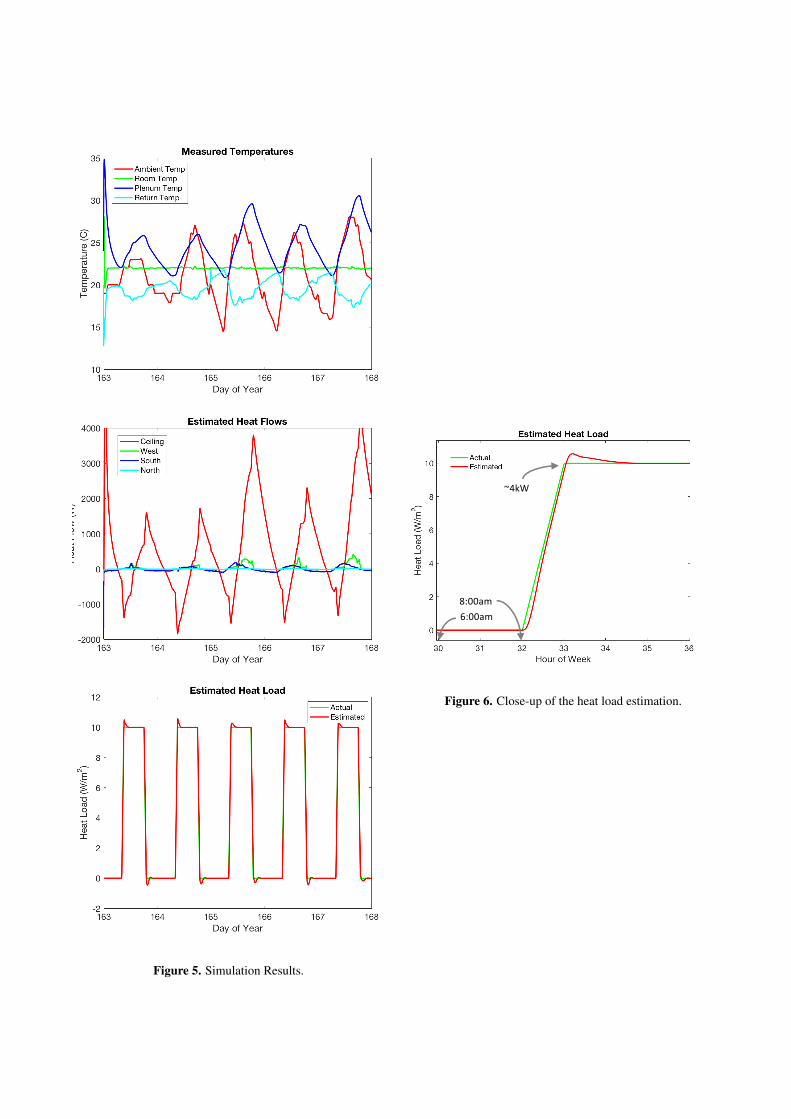
Figure 5. Simulation Results.

6:00am8:00am

~4kW

Figure 6. Close-up of the heat load estimation.