JOURNAL OF MULTIVARIATE ANALYSIS 9, 531-544 (1979)

An Identity for the Wishart Distribution with Applications*

L. R. HAFF

University of California, San Diego

Communicated by M. Rosenblatt

IJet s,,, have a Wishart distribution with unknown matrix X and K degrees of freedom. For a matrix T(S) and a scalar h(S), an identity is obtained for Eztr[h(S) TX-i]. Two applications are given. The lirst provides product moments and related formulae for the Wishart distribution. Higher moments involving S can be generated recursively. The second application concerns good estimators of 6 and Z-i. In particular, identities for several risk functions are obtained, and estimators of X (X-i) are described which dominate aS(bS-I), a < l/K (b < k - p - 1). Half [(1977) J. Multivar. Anal. 7 374-385; (1979) Ann. Statist. 7 No. 5; (1980) Ann. Statist. 8 used special cases of the identity to find unbiased risk estimators. These are unobtainable in closed form for certain natural loss functions. In this paper, we treat these case as well. The dominance results provide a unified theory for the estimation of Z and 2-i.

1. INTRODUCTION

Let S,X, have a Wishart distribution with unknown matrix Z and k degrees of freedom. In the standard notation, S - W(Z, k), ES = kE. For a possibly nonsymmetric T,x, = (T,,(S)) and a scalar h(S), an identity is obtained for I@(S) tr(T,ZY)]. This identity (given by (2.1)) and two applications are the

subject of this paper. The identity generalizes some special cases which appear in Haff [3] and [4].

It is derived from Stokes’ Theorem, a multivariate integration by parts. Stein [14] introduced the integration by parts idea within the context of estimating the multivariate normal mean. He did not use Stokes’ Theorem, but certain other generalizations of the Fundamental Theorem of Calculus.

The first application (Section 3) generates product moments and related formulae for the Wishart distribution. As usual, denote S by (Q) and S-l by (sij). Olkin and Rubin [lo] gave a method for computing Wishart moments by

Received May 2, 1978; revised June 25, 1979.

AMS 1970 subject classifications: Primary 62FlO; Secondary 62C99. Key words and phrases: Wishart and inverted moments, estimation of covariance

matrix and its inverse, Stoke’s theorem, general identities for the risk function.

531 0047-259x/79/040531-14$02.00/0

Copyright 0 1979 by Academic Press, Inc. All rights of reproduction in any form reserved.

532 L. R. HAFF

symmetry. Later, Kaufman [7] computed the moments E(sijs”z) by exploiting the factorization S = L’L, L a lower triangular matrix. In essence, he used the results of Olkin [9] to obtain the distribution of L-l. Kaufman’s results were given for a class of generalized Wishart distributions. Martin [8] obtained the same moments by using characteristic functions. Our method of computing inverse Wishart moments is easier than either of these. For positive integers i,i, 12, I (all <p), we obtain (Es”s (3 kr, Esiksjl, EsiVk) as the solution of a non- singular system of linear equations. The higher moments involving S can be obtained recursively.

Section 4 presents the second application for the identity. Its results extend and unify some of my previous work on estimating Z and Z-l-see [3], [4], and [5]. Throughout, if an estimator 2 incurs loss&$ zl), then the risk R($ Z) = EL($, Z) is an average over the W(Z, k) distribution. The natural estimators of Z(,?Y) are

as, 0 < a < l/k

(bS-1, O<b<k--p-l) (l-1)

with a = l/k (b = k - p - 1) specifying the unbiased estimator. Here, we provide estimatorsz(z-l) which dominate aS(h’F) for .a variety of loss functions. Roughly speaking, our estimators have the form

2 = a(S + ut(u)l)

p-1 = b(S-1 + vt(w)I)] (14

in which t(.) is nonnegative, bounded, and nonincreasing; and u(v) is the arithmetic, geometric, or harmonic mean eigenvalue of S(S-l). The precise conditions are found in Subsection 4.2. In [3], [4], and [5], special cases of (2.1) were used to obtain an unbiased estimator for the risk function. It was obtained in certain cases in which the loss function depended on Z-i explicitly. Typical cases were L(z, Z) = tr(&Pl - 1)2 and L@l, 2-l) = tr(,% - Z-‘)“Q with Q an arbitrary p.d. matrix. In the present paper, the unbiased risk estimator is obtained for other loss functions of this type. Also, some useful identities are provided for loss functions not of this type, e.g.,

L(2, Z) = c (6,j - CQ)” pij . (1.3) i@

Given (1.3) the unbiased risk estimator is unobtainable in closed form unless Bij = asij (i,j = l,..., p). From the risk identities, we impose conditions on t(.) under which ,@%) dominates aS(bS-l).

This paper was the subject of two talks given by me at Stanford University during February 1978. At that time, I learned of Charles Stein’s unpublished results in this area. Among these results is the identity (2.1), which he essentially

IDENTITY FOR THE WISHART DISTRIBUTION 533

derived several years ago. My derivation is independent and quite distinct from his-see Section 2 for further comment.

Subsection 4.1 is a brief review of the literature concerning the estimation of .Z and P-l.

2. AN IDENTITY FOR THE WISHART DISTRIBUTION

Let M = (miP(S)) be a p x p matrix. The identity is stated in terms of the following definitions:

DEFINITION 2.1. (Off-diagonal multiplication) The matrix M(,, = (m&) is such that

I rnij = maj i=j

= cmij i#j. I

Whenever (c) follows inversion, i.e., (M-l)(,) , we simply write ML-l). Note that tr[M(,$V~,,,J = tr(MIV), c # 0, for all p x p matrices M and IV.

DEFINITION 2.2. (Matrix divergence) D*M = ZZ am,,/&, . 1

DEFINITION 2.3. (The usual norm) 11 M 11 E [ZZm~j]l/z. 1

Our identity for the Wishart distribution is now given by

THEOREM 2.1. For a matrix TpX, = (T,,(S)) and a scalar h(S), assume that

(i) the functions T,(S) h(S) satisfy th e conditions of Stokes’ theorem on . all regions

W = %P,, ~4 = {S: S Z 0 (p.s.d.), 0 -=c ~1 < II S II < PJ;

(ii) on b,(W) = {S: S >, 0, I( S (1 = pr},

as p1 -+ O+; and

(iii) on b,(W) = {S: S > 0, 11 S (1 = pz},

s;~~~, I h(S)1 II T II = ob?‘k’2 exph41

as pz + 00 for arbitrary m > 0.

534 L. R. HAFF

Then we have

E[h(S) tr(TF)] = 2E[h(S) D*TclizJ + 2E tr [w . Ttl,2)]

+ (K - p - 1) E[h(S) tr(S-lT)], (2.1)

provided the integrals exist.

Remark 1. See Half [3] and [4] for particular applications of Stokes’ theorem on the p.s.d. matrices and a brief description of the geometry. Stokes’ theorem concerns regions W, more general than ours, and scalars g(S) for which

Here b(B?) is the boundary of W, cos qij the direction cosine at S E b(W) associated with (i,j), and dT differential surface area. Regarding condition (i) (or the validity of (2.2)) th e reader might consult Whitney [17], p. lOOff. Whitney’s conditions are more general than needed for the applications in the present paper.

Remark 2. Stein’s unpublished proof of (2.1) is based on certain identities for the normal distribution-see [14], pp. 377-379. A geometric proof, which is somewhat more direct, is obtained by extending the work in [3], pp. 377-379. It entails an application of (2.2) on the cone of p.s.d. matrices. We shall omit the details.

3. COMPUTATION OF WISHART MOMENTS

In this section, the identity (2.1) is used to compute second order moments for the Wishart and inverted Wishart distributions. Also, we derive some related equations. The second moments are well known-see Press [12, chapter 51 for a convenient summary. Here we do the computations in a relatively efficient manner.

We need the following from [4] and [S]:

LEMMA 3.1. If QDx, is an arbitrary matrix of constants, then

(i> ~*(sQ)(l~ = (w) tr Q,

@) D*(S2Qh) = (w) tr(SQ) + (1/2)(tr S)(tr Q), and

(iii) D*(S-rQ)(r12) = -(l/2) tr(SFQ) - (1/2)(tr S-r)(tr S-lQ).

IDENTITY FOR THE WISHART DISTRIBUTION 535

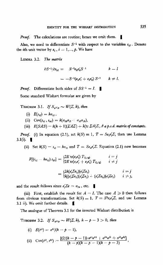
Proof. The calculations are routine; hence we omit them. 1

Also, we need to differentiate S-l with respect to the variables stj . Denote the ith unit vector by ei , i = l,..., p. We have

LEMMA 3.2. The matrix

as-l/as,, = --S-le,e;S-l k=l

= -S-‘(eke; + eleL) S-l k # 1.

Proof. Differentiate both sides of SS-i = I. 1

Some standard Wishart formulae are given by

THEOREM 3.1. If S,Q, - W(Z: k), then

(i) E(Q) = kuii ,

(ii) COV(S,~ , ski) = k(uikujt + UUU~~C),

(iii) E(SAS) = k(k + l)(CAZ) + k(tr .EA)Z, A ap.s.d. matrix of constants.

Proof. (i) In equation (2.1), set h(S) = 1, T = Seie;Z, then use Lemma 3.1(i). 1

(ii) Set h(S) = sii - kuii and T = Se,eiZ. Equation (2.1) now becomes

I

2k(eiZk,)(etZe,) i=j

= k[(eiZee,)(eiZej) + (e:Zee,)(e;Zej) i #.I,

and the result follows since e;Ze = uj, , etc. i

(iii) First, establish the result for A = I. The case A > 0 then follows from obvious transformations. Set h(S) = 1, T = S2eie;Z, and use Lemma 3.1 ii). We omit further details. 1

The analogue of Theorem 3.1 for the inverted Wishart distribution is

THEOREM 3.2. If S,X, - W(Z, k), k - p - 3 > 0, then

(i) E(sij) = &/(k -p - I),

536 L. R. HAFF

(4

+ (k - p)(kl- p - 3) z-lAz-l,

A a p.s.d. matrix of constants.

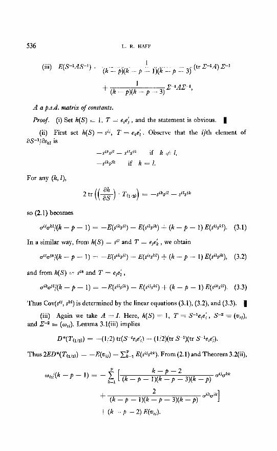
Proof. (i) Set h(S) = 1, T = eieJ , and the statement is obvious. 1

(ii) First set h(S) = @j, T = eke; . Observe that the ijth element of as-l/as,, is

-siksjl _ silsjk if kfl, -sikSjk if k = 1.

For my (k, Q

2 tr ((-$) . T(,,,)) = -siW - sizsjk

so (2.1) becomes

&“Z/(k - p - 1) = --E(sV) - E(sizsjk) + (k - p - 1) E(s%“~). (3.1)

In a similar way, from h(S) = siz and T = ejeL , we obtain

,iZ,jk/(k - p - 1) = -E(si”sjz) - E(sijskz) + (k - p - 1) E(sizsjk), (3.2)

and from h(S) = sik and T = eje; ,

,iW/(k - p - 1) = -E(sW) - E(sijskL) + (k - p - 1) E(siksjz). (3.3)

Thus Cov(#j, skz) is determined by the linear equations (3.1), (3.2), and (3.3). a

(iii) Again we take A = I. Here, h(S) = 1, T = S-le,ei , S-2 3 (vii),

and P2 = (wii). Lemma 3.l(iii) implies

D*( T(llz)) = -(l/2) tr(S2eie>) - (1/2)(tr S-l)(tr S-Q&).

Thus 2ED*(T(,,,)) = --E(Q) - -& E( sijskk). From (2.1) and Theorem 3.2(ii),

+ (k - p - l)(k ” p - 3)(k - p) ozka’k 1 + (k - P - 2) E(v,j)*

IDENTITY FOR THE WISHART DISTRIBUTION 531

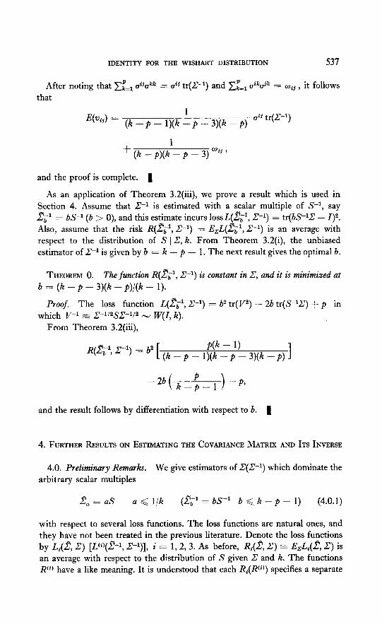
After noting that C%, oijokk = & tr(C-l) and Cz=‘=, &rjk = wij , it follows that

and the proof is complete. 1

As an application of Theorem 3.2(iii), we prove a result which is used in Section 4. Assume that Z-l is estimated with a scalar multiple of S-r, say 2;’ = R-r (b > 0), and this estimate incurs 10ssL(,&~, 2-l) = tr(bS-lZ - 1)2. Also, assume that the risk R(z;‘, 2-l) = E,L@;‘, 2-l) is an average with respect to the distribution of S 1 Z, k. From Theorem 3.2(i), the unbiased estimator of Z-l is given by b = k - p - 1. The next result gives the optimal b.

THEOREM 0. The function R(,!?;‘, Z-l) is constant in Z, and it is minimized at b = (k - p - 3)(k - p)/(k - 1).

Proof. The loss function L@;‘, Z-l) = b2 tr(V2) - 2b tr(S-lZ) + p in which V-1 E: ~-112,9~-1/2 - W(I, k).

From Theorem 3.2(iii),

R(‘?f ‘-‘) = b2 [ (k _ p - l$?;’ 3)(k - p) ]

and the result follows by differentiation with respect to b. 1

4. FURTHER RESULTS ON ESTIMATINGTHE COVARIANCE MATRIX AND ITS INVERSE

4.0. Preliminary Remarks. We give estimators of Z(.J-‘) which dominate the arbitrary scalar multiples

2, = aS a ,( l/k (2;‘=bS-’ b<k--p-l) (4.0.1)

with respect to several loss functions. The loss functions are natural ones, and they have not been treated in the previous literature. Denote the loss functions by I+(,$ Z) [Lo)(%l, ,P)], i = 1,2, 3. As before, Ri($ Z) = E&@, Z) is an average with respect to the distribution of S given Z and k. The functions R(i) have a like meaning. It is understood that each R,(Rci)) specifies a separate

538 L. R. HAFF

estimation problem. Let Z and z* be competing estimators of 2. As usual, we have “2 dominates ,?‘,(modL,)” if I&($ Z) < &(z’, , Z) (VZ).

Our results provide a unified theory for estimating Z and its inverse. For a variety loss functions, we dominate ,&(&l) by certain estimators

2 = a[S + ut(u)l] (2-l = b[S-1 + wt(w)l]) (4.0.2)

in which t(.) is a nonincreasing function of an average eigenvalue of S(S-l). The average eigenvalue U(W) might be the arithmetic average (tr S)/p [tr(S-l)/p], the geometric average j S l1/P [I S l-1/P], or the harmonic average p/tr(S-t) [p/tr Sj. Our choices t(.) and U(W) will depend on the loss function.

4.1. History. First we describe some of the known results for

L,(2, Z) = tr(,ZY) - log 1 ZZ-l 1 - p;

L,@, 2) = tr(.D--l - 1)2; (4.1.1)

-%tfj, 2) = c @ii - 4” 4ij 9 i<j

with qii > 0 an arbitrary set of weights; and

L(O)(z-1, z-1) = tr(z-1 - z-1)2 S;

L(l)(z-1, z-1) = tr(z-1 - Z-l)2 Q, (4.1.2)

Q an arbitrary p.d. matrix. Let /I be a positive scalar. Stein [6] showed that all estimators of the form jI(S/K) are inadmissible with respect to L, . Selliah [13] gave the same result for L, . Perlman [ll] showed that if (Kp - 2)/(kp + 2) < p < 1, then /3(S/k) dominates S/k with respect to L, , qii = 1, i < j. In these papers, the estimators are only slightly better than S/k. Stein [15] presented an estimator which is substantially better, again under L, . Regards to the estimation of Z-l, Efron and Morris [2] studied the estimators zajl = as-’ + [b/tr(S)]I, a, b > 0, and proved that if a = k - p - 1 and b = p2 + p - 2, then 2;: dominates zil under L(O). See, also, Stein, Efron and Morris [16]. In Haff [3], the estimator ,??a;’ was generalized as 2;’ = as-l + [r(w)/tr(S)]I for w = p 1 S Il/“/tr(S), real Y(W). Then conditions were given under which.&’ dominates &’ for both L(O) and L(l). Although 2~’ dominates (k - p - l)S-r(modL(‘J)), it was shown [3] that (k - p - l)S-’ dominates r,-,’ (mod L(l)). The reversal is troublesome because L(O) and L(l) are qualitatively close if Q = RZ and k is large. Haff [4] studied yet a larger class 2;: = [a + f(S)]S-l + g(S)1 (f(S) and g(S) real) and g ave conditions under which 2;: dominates E;‘(mod L(l)). In particular, results were given for f(S) = -m(w) and g(S) = r(w)/tr(S), 0 < Y(W) < 1. A more recent paper [5] proposed estimators of the form (4.0.2), u = p/tr(S-l). These were given an Empirical Bayes interpretation, and condi- tions were established for their dominance of aS under both L, and L, .

IDENTITY FOR THE WISHART DISTRIBUTION 539

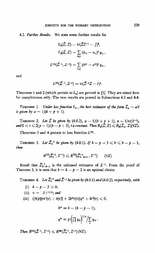
4.2. Further Results. We state some further results for

L,@, Z) = tr@P - /)2,

L,(Z q = c @, - %y qij , d(i

and

L(Q(z-1, z-1) = 1 (6.i) - 42 qii ,

i<i

L(3+2-1, 2-l) = tr(,ElL! - 1)2.

Theorems 1 and 2 (which pertain to La) are proved in [5]. They are stated here for completeness only. The new results are proved in Subsections 4.3 and 4.4.

THEOREM 1. Under loss function L, , the best estimator of the form 2, = aS isgiven by a = l/(K+p+ 1).

THEOREM 2. Let L? be given Sy (4.0.2), a = l/(K + p + l), u = l/tr(S-l), andO < t < 2(p - 1)/(/z - p + 3), t a constant. Then R&I?, C) < I&(&, zl)(VZ).

Theorems 3 and 4 pertain to loss function Lc2).

THEOREMS. Let,&y1begivenby(4.0.1).Ifh-p-3<b<h-p-l, then

Rt2)(&l, Z-‘) < R(2)(,&1 , Z-‘) wo

Recall that .&~,,-, is the unbiased estimator of Z-l. From the proof of Theorem 3, it is seen that b = k - p - 2 is an optimal choice.

THEOREM 4. Let f;bl adz-1 be given by (4.0.1) and (4.0.2), respectively, with

(i) k-p-3 >O;

(ii) v = ] S ]-l/P; and

(iii) #/P)[vt’(v) + t(v)] + B*t(v)}q* + bt2(v) d 0,

b*=b-(h-p-l),

Then R’2’(%, Z-l) < R’2’(z:,-1, Z-l) (VZ).

540 L. R. HAFF

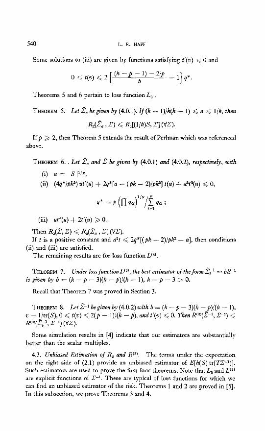
Some solutions to (iii) are given by functions satisfying t’(n) < 0 and

0 :< t(v) < 2 [ (~-P-11)-2/P b

- l] q”.

Theorems 5 and 6 pertain to loss function L, .

THEOREM 5. Let ,fm begiven by (4.0.1). I f (K - l)/K(k + 1) < a < l/k, then

R,<Z , q < R3[(W)S, z:l (V-q.

If p > 2, then Theorem 5 extends the result of Perlman which was referenced

above.

THEOREM 6. , Let za and 2 be given by (4.0.1) and (4.0.2), respectively, with

(i) u = 1 S Ilip;

(ii) (4q*/ph2) ut’(u) + 2q*[a - (pk - 2)/pP] t(u) + u2t2(u) < 0,

(iii) d”(u) + 2t’(u) 2 0.

Then Ra($ 2) < -R,(za, .Z) (VZ). I f t is a positive constant and a’9 < 2q*[(pk - 2)/pK2 - a], then conditions

(ii) and (iii) are satisfied. The remaining results are for loss function L13).

THEOREM 7. Under loss function Lt3J, the best estimator of the form 2-l =.= bS-1 is given by b = (h - p - 3)(k - p)/(h - l), k - p - 3 > 0.

Recall that Theorem 7 was proved in Section 3.

THEOREM 8. Let 2-l begiven by (4.0.2) with b = (k - p - 3)(k - p)/(k - l), v = l/tr(S), 0 < t(v) f 2(p - I)/(k - p), and t’(v) < 0. The-n R(3)(z-1, Zm ‘) < R’3’(2y, Z-1) (Vz?Y).

Some simulation results in [4] indicate that our estimators are substantially better than the scalar multiples.

4.3. Unbiased Estimation of R, and Rt2). The terms under the expectation on the right side of (2.1) provide an unbiased estimator of E[h(S) tr( TZ-I)]. Such estimators are used to prove the first four theorems. Note that L, and Lc2’ are explicit functions of Z-l. These are typical of loss functions for which we can find an unbiased estimator of the risk. Theorems 1 and 2 are proved in [5]. In this subsection, we prove Theorems 3 and 4.

IDENTITY FOR THE WISHART DISTRIBUTION 541

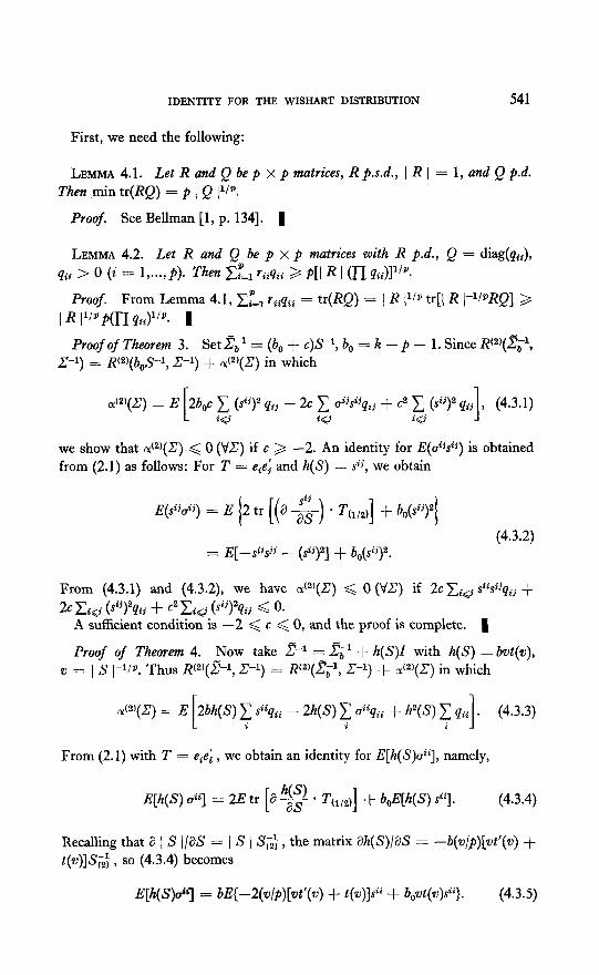
First, we need the following:

LEMMA 4.1. Let R and Q be p x p matrices, R p.s.d., 1 R 1 = 1, and Q p.d. Then min tr(RQ) = p ( Q jllp.

Proof. See Bellman [l, p. 1341. 1

LEMMA 4.2. Let R and Q be p x p matrices with R p.d., Q = diag(q& qii > 0 (i = l,...,p). Then Xi”=, r,,q,, > p[l R I (n q#p.

Proof. From Lemma 4.1, X:=1 riiqii = tr(RQ) = j R IlIp tr[[ R l-l/pRQ] >

I R VP P(I-I qiiY. I

Proof of Theorem 3. Set 2;’ = (b, + c)S-I, b, = h - p - 1. Since R(z)(&l, Z-1) = R(2)(b,S-l, Z-1) + P(Z) in which

cG)(,Z) = E 2b,c 1 (@)” qij - 2~ C uijsijqij + c2 C (sij)” qij , (4.3.1) iQ i(j is5 1

we show that CY.(~)(Z) < 0 (Vi?) if c > -2. An identity for I?(&@) is obtained from (2.1) as follows: For T = eiei and h(S) = sij, we obtain

E(sij&) = E 2 ( tr [(a -$) * Tw2)] + M@)21

= E[-si$jj _ (sij)2] + b,($i)2. (4.3.2)

From (4.3.1) and (4.3.2), we have LX(~)(Z) < 0 (VZ) if 2c Cici siisjjqij +

2C Ci<j (Si5)2qi’ij + C2 xi@ (Sii)2qij < 0. A sufficient condition is -2 < c < 0, and the proof is complete. 1

Proof of Theorem 4. Now take 2-l = 2;’ + h(S)1 with h(S) = bwt(w), v = 1 S I-l/r’. Thus R(2@-l, Z-’ ) = Rt2)(zc1, Z-l) + ,t2)(Z) in which

LX(~)(Z) = E 2bh(S) T siiqi, - 2h(S) C aiiq,i + h’(S) 1 qii . (4.3.3) i i I

From (2.1) with T = e,e; , we obtain an identity for E[h(S)@], namely,

E[h(S) uii] = 2E tr [a g * T(,,,)] + b,E[h(S) sii]. (4.3.4)

Recalling that a / S l/W = 1 S ) 5’~; , the matrix ah(S)/% = -b(w/p)[wt’(w) + t(o)]SGt , so (4.3.4) becomes

E[h(S)&J = bE{--2(w/p)[wt’(w) + t(w)]sii + bowt(w)sii}. (4.3.5)

542 L. R. HAFF

From (4.3.3) and (4.3.5), we obtain an unbiased estimator of c&s)(Z),

6Y2’(2) = bv[(4/~9(wt’(v) + t(w)) + 2b*t(w)] c siiqii + bv[bwt2(v)] ; qii . (4.3.6) i

We have C?(~)(Z) < 0 if and only if [(4/p)(vt’(v) + t(w)) + 2b*t(w)][x, Siiqii/Ci qiJ + bwt2(w) < 0. A su ffi cient condition for the last inequality is [(4/p)(wt’(w) + t(w)) + 2b*t(w)] wq* + bwt2(w) < 0 ( see Lemma 4.2), and the proof is com- plete. 1

4.4. Exploitations of the Identity for R, and Rc3). Here we prove Theorems 5, 6, and 8. Recall that L, and L(s) are explicit functions of Z (rather than Z-l). We illustrate, here, the utility of (2.1) in natural situations where an unbiased estimator of R is unobtainable.

Proof of Theorem 5. Set zG = (a, - d)S, a0 = l/K, and d > 0. We have R,(.& , Z) = %(a$, 2:) + aa in which

05(z) = E (--2ad zj sfjqij + 2d zj sijuijqij + d2 zj ski j)* (4.4.1)

We use an identity for E(sijuij) which is given by (2.1) with T = 5’eieiZ and h(S) = sij . Note that D*T c1j2) = ((P + 1)/2) tr(eie$:) = ((P + 1)/2) *ij (recall Lemma 3.1(i)) and 2 tr[a(h(S)/aS) . T(1,2j] = siju<j + siiuji . NOW (2.2) becomes

E(S:) = (h + 1) E(siju,j) + E(siiojj). (4.4.2)

If we solve (4.4.2) for E(sijqij) and apply the result to (4.4. l), we obtain as(Z) = E{--;?d[l/h - l/(h + I)] + d”>{& s&ij} - E{[2d/(h + I)] &jSiioj*qij .There- for (Y&Z) < 0 (VZ) if -2d[l/k - l/(K + I)] + d2 < 0 or, equivalently, d < 2/k(k + 1). Since a = a, - d, we finally obtain the sufficient condition (k - l)/ h(h + 1) Q a < l/k. 1

Proof of Theorem 6. Here 2 = 2, + m(u)l, m(u) = aut(u), and R,($ Z) =

R,(% 9 -V + 4J3

05(Z) = E Pam(u) i siiqii - 2m(~) i uiiqii + m”(u) i qii]. (4.4.3) id i-l i-1

For T = Se,e;Z and h(S) = m u we have D*T(,,,) = ((p + 1)/2)aii and ( ), ah(S)/% = [um’(u)/plS;t . Now the identity (2.1) becomes

E[m(u)sii] = hE[m(u)uii] + (2/p) E[um’(u)]ue . (4.4.4)

Another application of (2.1) with h(s) = urn’(u) gives

E[um’(u)sii] = KE[um’(u)aii] + (2/p) E{u[um’(u)]‘crii}. (4.4.5)

IDENTITY FOR THE WISHART DISTRIhUTION 543

From (4.4.4) and (4.4.5), E[m(u)s,,] = kE[na(u)oJ + (2/p) E[(l/k)um’(u)sii - (2/pk) u(um’(u))‘aji] . Aft er solving the last equation for E[m(u)aii] and applying

the result to (4.4.3), we obtain %(.Z) = E[2um(u) - (2/K) m(u) + (4/pP)um’(u)] .

LX;=, wil - @/Pk”) * W~M4)‘lEi”E~ ai&il + E[m2(u)lEkl Gil* If m(u> (= aut(u)) satisfies condition (iii), then aa(Z) < 0 (VZ) if [2um(u) - (2/k) m(u) + (4/pk2) um’(u)][C~!r sdiqii] + [m2(u)][~~‘1 &I < 0. An application of Lemma 4.1 and simple algebra shows that condition (ii) is sufficient for the latter inequality.

We omit further details. 1

Proof of Theorem 8. We have 2-l = 2;’ + h(S)I, h(S) = Kit, and

z, = l/tr(S). Thus L(s)(,I-l, Z-l) = U3)(z$, Z-l) + OC(~)(Z),

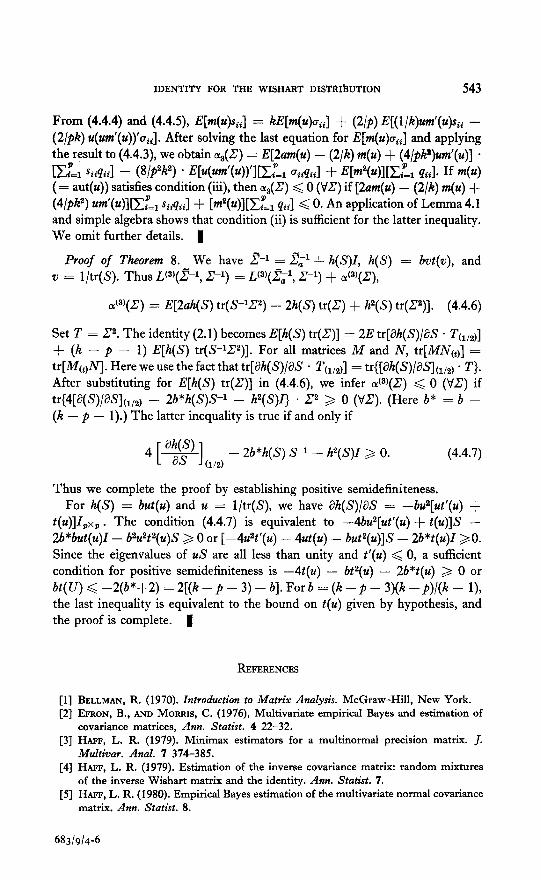
U(~)(Z) = E[2ah(S) tr(S-‘Z2) - 2h(S) tr(Z) + h2(S) tr(Z2)]. (4.4.6)

Set T = Z2. The identity (2.1) becomes E[h(S) tr(Z)] = 2E tr[ah(S)/X? . T(l,2)] + (k - p - 1) E[h(S) tr(S’-lZ2)]. F or all matrices M and N, tr[MNuJ = tr[M(,$VJ Here we use the fact that tr[ah(S)/&S . T(,,,)] = tr{[ah(S)/&Sl(,,,) . T}. After substituting for E[h(S) tr(Z)] in (4.4.6), we infer Ok < 0 (VZ) if tr{4[Z+(S)/&S](1,2) - 2b*h(S)S-l - h2(S)I) . Z2 3 0 (VZ). (Here b* = b - (k - p - l).) The latter inequality is true if and only if

4 rwl(l,2) - 2b*h(S) s-1 - h2(S)I > 0.

Thus we complete the proof by establishing positive semidefiniteness. For h(S) = but(u) and u = l/tr(S), we have ah(5’)/iW = --bu2[ut’(u) +

Wl~~X1) * The condition (4.4.7) is equivalent to -4&a[z&(u) + t(u)]S - 2b*but(u)l- b2u2t2(u)S > 0 or [-4u2t’(u) - 4ut(u) - bz&(u)]S - 2b*t(u)l >O. Since the eigenvalues of US are all less than unity and t’(u) < 0, a sufficient condition for positive semidefiniteness is -4t(u) - bP(u) - 2a*t(u) > 0 or

bt( U) < -2(b*+2) = 2[(k - p - 3) - b]. For b = (k - p - 3)(k - p)/(k - l), the last inequality is equivalent to the bound on t(u) given by hypothesis, and the proof is complete. 1

REFERENCES

[l] BELLMAN, R. (1970). Introduction to Matrix Analysis. McGraw-Hill, New York. [2] EFRON, B., AND MORRIS, C. (1976), Multivariate empirical Bayes and estimation of

covariance matrices, Ann. Statist. 4 22-32. [3] HAFF, L. R. (1979). Minimax estimators for a multinormal precision matrix. J.

Multivm. Anal. 7 374-385. [4] HAFF, L. R. (1979). Estimation of the inverse covariance matrix: random mixtures

of the inverse Wishart matrix and the identity. Ann. Statist. 7. [5] HAFF, L. R. (1980). Empirical Bayes estimation of the multivariate normal covariance

matrix. Ann. Statist. 8.

683/9/4-C

544 L. R. HAFF

[6] JAMES, W., AND STEIN, C. (1961). Estimation with quadratic loss. In Fourth Berkeley Symposium Math. Statist. Prob. Univ. of California Press, Berkeley.

[7] KAUFMAN, G. M. (1967). Some Buyesian Moment Formulae. Report No. 6710, Center for Operations Research and Econometrics. Catholic University of Louvain. Heverlee, Belgium.

[8] MARTIN, J. (1965). Some moment formulas for multivariate analysis. Unpublished. [9] OLKIN, I. (1950). A class of integral identities with matrix argument. Duke Math. J.

26 207-213. [lo] OLKIN, I., AND RUBIN, H. (1962). A characterization of the Wishart distribution.

Ann. Math. Statist. 33 1272-1275. [ll] PERLMAN, M. D. (1972). R d e uced mean square estimation for several parameters.

Sunkhya 34 89-92. [12] PRESS, S. J. (1972). Applied Multz’waviate Analysis. Holt, Rinehart & Winston,

New York. [13] SELLIAH, J. (1964). Estimation and Testing Problems in a Wishart Distribution.

Ph. D. thesis, Department of Statistics, Stanford University. [14] STEIN, C. (1973). Estimation of the mean of a multivariate normal distribution.

In Proceedings Prague Symp. Asymptotic Statist. pp. 345-381. [15] STEIN, C. Reitz lecture. Thirty-eighth Annual meeting, IMS. Atlanta, Georgia. [16] STEIN, C., EFRON, B., AND MORRIS, C. (1972). Improving the usual estimator of a

normal Couariance matrix. Technical Report No. 37, Department of Statistics Stanford University.

[17] WHITNEY, H. (1957). Geometric Itztegration Theory. Princeton Univ. Press, Princeton, N. J.