Embed Size (px)
Citation preview

HAL Id: hal-00765296https://hal-supelec.archives-ouvertes.fr/hal-00765296
Submitted on 14 Dec 2012
HAL is a multi-disciplinary open accessarchive for the deposit and dissemination of sci-entific research documents, whether they are pub-lished or not. The documents may come fromteaching and research institutions in France orabroad, or from public or private research centers.
L’archive ouverte pluridisciplinaire HAL, estdestinée au dépôt et à la diffusion de documentsscientifiques de niveau recherche, publiés ou non,émanant des établissements d’enseignement et derecherche français ou étrangers, des laboratoirespublics ou privés.
An imprecision importance measure for uncertaintyrepresentations interpreted as lower and upper
probabilities, with special emphasis on possibility theoryR. Flage, Terje Aven, Piero Baraldi, Enrico Zio
To cite this version:R. Flage, Terje Aven, Piero Baraldi, Enrico Zio. An imprecision importance measure for uncertaintyrepresentations interpreted as lower and upper probabilities, with special emphasis on possibilitytheory. Proceedings of the Institution of Mechanical Engineers, Part O: Journal of Risk and Reliability,SAGE Publications, 2012, 226 (6), pp.656-665. �10.1177/1748006X12467591�. �hal-00765296�

An imprecision importance measure for uncertainty representations
interpreted as lower and upper probabilities, with special emphasis on
possibility theory
R. Flage1, T. Aven
1, P. Baraldi
2& E. Zio
3,2
1 University of Stavanger, Norway
2 Polytechnic of Milan, Italy
3Chair on Systems Science and the Energetic Challenge, European Foundation for New Energy-Electricité de
France, EcoleCentrale Paris and Supelec, France
Uncertainty importance measures typically reflect the degree to which uncertainty
about risk and reliability parameters at the component level influences uncertainty
about parameters at the system level. The definition of these measures is typically
founded on a Bayesian perspective where subjective probabilities are used to express
epistemic uncertainty; hence, they do not reflect the effect of imprecision in
probability assignments, as captured by alternative uncertainty representation
frameworks such as imprecise probability, possibility theory and evidence theory. In
the present paper, we define an imprecision importance measure to evaluate the effect
of removing imprecision to the extent that a probabilistic representation of uncertainty
remains, as well as to the extent that no epistemic uncertainty remains. Possibility
theory is highlighted throughout the paper as an example of an uncertainty
representation reflecting imprecision, and used in particular in two numerical
examples which are included for illustration.
Key words: imprecision; importance measure; epistemic uncertainty

1 Introduction
The use of importance measures (IM) is an integral part of reliability and risk analysis. IM are
used to study the effect on system level reliability or risk parameters of altering component
level parameters. A number of uncertainty importance measures (UIM) have also been
proposed in the literature (Aven &Nøkland, 2010). These extend the ‘classical’ reliability and
risk IM in the presence of epistemic uncertainty. UIM are used to study to what degree
uncertainty about risk and reliability parameters at the component level influences uncertainty
about parameters at the system level.
In general terms, we are interested in the quantity Y, possibly a vector, and introduce a model
g(X) which relates n input quantities X = (X1,X2,…,Xn) to the output quantity of interest Y. In
particular,we are interested in an output quantity Y= p = g(q), function of the input X=q
where p and q are reliability or risk parameters at the system and component level,
respectively. Typically, p and q are given the interpretation of long-run frequencies, e.g. the
fraction of time a system and its components are functioning, respectively. This is the
interpretation adopted, for example, in the probability of frequency approach to risk analysis
(Kaplan & Garrick, 1981).
Classical IM are used to analyze changes to p given changes to q. For example, the so-called
‘improvement potential’ of component i is defined as the change to the system availability p
when the component availability qi is set equal to 1, and the Birnbaum IM is defined as the
partial derivative of p with respect to qi(e.g. Aven & Jensen, 1999; Rausand&Høyland, 2004).
UIM are typically founded on a Bayesian perspective. A subjective probability distribution F
is introduced for q and propagated through a model g. The result is a probability distribution
of p, and UIMs are used to analyse changes to the distribution of p given changes to F.
Reference is made to Section 2 for a brief review of IM and UIM.
In a Bayesian perspective subjective probabilities express epistemic uncertainty; hence, they
do not reflect imprecision in probability assignments. The term imprecision here labels the
phenomenon captured by a wide range of extensions of the classical theory of probability,
including lower and upper pre-visions (Walley, 1991), belief and plausibility functions

(Dempster, 1967; Shafer, 1976), possibility measures (Dubois &Prade, 1988), fuzzy sets
(Zadeh, 1965), robust Bayesian methods (Berger, 1984), p-boxes (Ferson et al., 2003) and
interval probabilities (Weichselberger, 2000).
One much studied type of UIM is that reflecting the effect on system level parameter
uncertainty of removing component level parameter uncertainty. For example, for a
probability distribution F of component level parameters q which propagated through a model
g induces a probability distribution of the system level parameter p, this type of UIM
evaluates changes to the distribution of p by assuming qi known for some i. Of course, the
value of qi cannot be specified with certainty and so the resulting measure becomes a function
of qi. An example is the measure Var(p) – Var(p|qi), expressing the reduction in the variance
of the system level parameter p that is achieved by specifying the value of the component
level parameter qi. One way to proceed is to consider the expected value of the above
measure, namely (Iman, 1987):
(1)
Aven & Nøkland (2010) investigate the link between UIM and traditional IM. In doing so
they distinguish between the cases that X and Y, as introduced above, are (a) observable
events and quantities, such as the occurrence of a system failure and the number of system
failures, and (b) unobservable parameters, such as p and q. Based on their findings a
combined set of IM and UIM is defined.
Within a non-probabilistic framework, a Fuzzy Uncertainty Importance Measure (FUIM) has
been proposed in (Suresh et al., 1996) to identify those component level parameters qi having
the greatest impact on the uncertainty of the system level parameter p. The FUIM measures
the distance between the output fuzzy sets considering the input parameters qi with or without
uncertainty. In (Baraldi et al., 2009), the FUIM has been modified in order to consider the
different imprecision in the output fuzzy sets, measured in terms of fuzzy specificity, instead
of the difference between the fuzzy sets. In (Liping & Fuzheng, 2009), an importance measure
based on the concept of possibilistic entropy has been proposed and applied to fault tree
analysis in a possibilistic framework.

In the present paper, we consider the case that a distribution pair Hq is introduced for q. We
may for example have Hq = [Nq, Πq], where Nq and Πq are the cumulative necessity and
possibility distributions (from possibility theory) of q, respectively; or Hq = [Belq, Plq], where
Belq and Plq are the cumulative belief and plausibility distributions (from evidence theory) of
q, respectively; or Hq = [Hql, Hq
u] where Hq
l and Hq
u are lower and upper imprecise
probability distributions of q, respectively. In the present paper, possibility theory is
highlighted throughout the paper as an example of an uncertainty representation reflecting
imprecision. The choice of possibility theory in this early study of the suggested IIM is due to
its mathematical simplicity; cf. Dubois (2006) who notes that ‘Possibility theory is one of the
current uncertainty theories devoted to the handling of incomplete information, more
precisely it is the simplest one, mathematically’.
Defining the imprecision of a distribution pair as the area between its lower and upper
cumulative distributions, we define an imprecision importance measure (IIM) that evaluates
the effect on system level parameter imprecision of removing component level parameter
imprecision. Two extents of imprecision removal are possible:
i. Removal of imprecision to the extent that a probabilistic representation remains
ii. Removal of imprecision to the extent that no epistemic uncertainty remains
The latter case may be seen as a special case of the former. The definition of an IIM in terms
of imprecision removal is associated with an analogous problem as was seen above for
uncertainty removal in the case of UIM; namely, the measure can be defined but neither the
specific value of a component level parameter nor its probability distribution can really be
specified. We are led to consider, respectively:
I. A probability distribution consistent with Hq
II. The IIM as a function of qi
In the following we refer to these as type I and type II measures. Flage et al. (2011) study the
type II measure. In the present paper,we extend the work of Flage et al. (2011) and study also
the type I measure in the case that Hq = [Nq, Πq]. A probability distribution is obtained from
Hq by considering a possibility-probability transformation procedure, and further
computations take place within the framework of a hybrid probabilistic/possibilistic method.

The remainder of the paper is organized as follows: In Section 2, we review some basic
classical IM and some UIM. In Section 3, we review the concepts of uncertainty and
imprecision, as well as their representation. In Section 4, we define an IIM as indicated above,
and in Section 5 the suggested measure is evaluated in terms of a numerical example where
possibility theory is used as the representation of uncertainty. Section 6 provides a discussion
and some conclusions.
2 Importance measures and uncertainty importance measures
There are essentially two fundamental classical importance measures: the ‘improvement
potential’ of a component, describing the effect on the system reliability of making the
component perfectly reliable; the Birnbaum importance measure, reflecting the effect on
system reliability of an incremental change in the reliability of a component. The
improvement potential of a component is defined by (e.g. Aven & Jensen, 1999; Rausand &
Høyland, 2004)
(2)
where h(q) is the system reliability function expressing p as a function of q; and h(1i,q) =
h(q1,...,1i,...qn) the system reliability function when component i is perfectly reliable. The
importance measures referred to as risk achievement worth (RAW) and risk reduction worth
(RRW) (e.g. Cheok et al., 1998; Rausand&Høyland, 2004; Zio, 2009) represent minor
adjustments of the improvement potential importance measure. The Birnbaum importance
measure is defined by (e.g. Aven & Jensen, 1999; Rausand & Høyland, 2004; Zio, 2009)
(3)
i.e. as the partial derivative of the system reliability with respect to qi. The improvement
potential importance measure is most relevant in the design phase of a system, whereas the

Birnbaum importance measure is most relevant in the operational phase (Aven& Jensen,
1999). See Rausand & Høyland (2004) and Zio (2009) for a more in-depth review of classical
IMs.
Uncertainty importance measures were described to some extent in Section 1. The UIM by
Iman (1987) is variance-based and hence an example of a measure in one of the three
categories described by Borgonovo (2006):
i. Non parametric techniques (input-output correlation)
ii. Variance-based importance measures
iii. Moment-independent sensitivity indicators.
See Borgonovo (2006) for a more in-depth review of UIMs.
3 Uncertainty, imprecision and its representation
In engineering risk analysis a distinction is commonly made between aleatory (stochastic) and
epistemic (knowledge-related) uncertainty (e.g. Apostolakis, 1990; Helton & Burmaster,
1996). Aleatory uncertainty refers to variation in populations. Epistemic uncertainty refers to
lack of knowledge about phenomena and usually translates into uncertainty about the
parameters of a model used to describe random variation. Whereas epistemic uncertainty can
be reduced, aleatory uncertainty cannot and for this reason it is sometimes called irreducible
uncertainty (Helton & Burmaster, 1996).
Traditionally, limiting relative frequency probabilities are used to describe aleatory
uncertainty and subjective probabilities are used to describe epistemic uncertainty. However,
as described in Section 1, several alternatives to probability as representation of epistemic
uncertainty have been suggested, the motivation being to capture imprecision in subjective
probability assignments. Imprecision here refers to inability to precisely specify a probability
(distribution). Presumably an analyst/expert would ideally want to characterize epistemic
uncertainty using a subjective probability (distribution); however, due to limitations in the
information available (e.g. lack of data, lack of phenomenological understanding) the
analyst/expert is unable or not willing to specify a single subjective probability (distribution)

and only able to or willing to specify a probability interval (a family of probability
distributions).
For example, numerical possibility distributions can encode special convex families of
probability measures (Dubois, 2006). In possibility theory, uncertainty and imprecision is
represented by a possibility function π. For each element ω in a set Ω, π(ω) expresses the
degree of possibility of ω. Since one of the elements of Ω is the true value, it is assumed that
π(ω) = 1 for at least one element ω. The possibility measure of an event A, Π(A), is defined
by
(4)
and the necessity measure of A, N(A), by
(5)
Uncertainty about the occurrence of an event A, then, is represented by the pair [N(A), Π(A)],
where the necessity and possibility measures can be given the interpretation of lower and
upper probabilities induced from specific convex sets of probability functions (Dubois, 2006):
(6)
Then, and (see e.g. Dubois & Prade, 1992).
Another point of view on possibility theory is a graded view where possibility measures
express the extent to which an event is plausible, i.e. consistent with a possible state of the
world, and necessity measures express the certainty of events. Reference is made to Dubois
(2006) and the references therein.
4 An imprecision importance measure

Consider the system level reliability or risk parameter p and its distribution pair Hp induced by
the propagation of the distribution pair Hq for a set of lower level parameters q through a
model g. Define the imprecision of a distribution pair H, denoted ΔH, as the area between its
lower and upper cumulative distributions, i.e.
(7)
as illustrated in Figure 1.
Figure 1.Imprecision measure ΔH equal to the area between the lower and upper distributions in the distribution
pair Hp.
For example, in the case of a distribution pair H = [N, Π] induced by a triangular possibility
distribution π with support S, we have – by geometrical considerations and recalling that a
possibility distribution has unit height – that the imprecision of the possibility distribution is
Δ(H) = |S| / 2. In the case of a probabilistic representation of uncertainty we have max H(x) =
min H(x) for all x, and hence ΔH = 0.
Now define Δi(Hp) as the imprecision of Hp when the imprecision of the distribution on the
parameter qi is removed. We may then define an imprecision removal importance measure
(IRIM) as

(8)
which expresses the amount of system level imprecision removal that comes from removing
imprecision at the component level. The relative imprecision removal effect can be studied in
terms of the measure
(9)
which expresses the fraction of imprecision associated with the distribution pair Hp that is
attributable to component i.
As described in Section 1, imprecision can be removed either to the extent that a probabilistic
representation remains, or to the extent that no epistemic uncertainty remains.
4.1 Type I measure
Removal of imprecision to the extent that a probabilistic representation remains means that
uncertainty about qi is described using a (subjective) probability distribution Fi(x) = P(qi ≤ x),
as illustrated in Figure 2.
Figure 2.Removal of imprecision (imprecise probability distribution – dashed lines) to the extent that a single-
valued probabilistic representation remains (solid line).

A probability distribution can be derived from a possibility distribution by considering a
possibility-probability transformation procedure. Then a hybrid probabilistic/possibilistic
method can be used for the joint propagation of the resulting probability distribution together
with the remaining possibility distributions. In the following we review a possibility-
probability transformation procedure based on Dubois et al. (1993) and a hybrid
probabilistic/possibilistic method based on Baudrit et al. (2006) and applied in the context of
risk analysis by (Baraldi&Zio, 2008).
4.1.1 Possibility-probability transformation procedure
Possibility-probability transformations (as well as probability-possibility transformations) are
based on given principles and ensure a consistent transformation to the extent that there is no
violation of the formal rules (definitions) connecting probability and possibility when
possibility and necessity measures are taken as upper and lower probabilities, and so that the
transformation is not arbitrary within the constraints of these rules. Nevertheless, as noted in
(Dubois et al., 1993):
... going from a probabilistic representation to a possibilistic representation, some information is lost
because we go from point-valued probabilities to interval-valued ones; the converse transformation adds
information to some possibilistic incomplete knowledge. This additional information is always
somewhat arbitrary.
When possibilityand necessity measures are interpreted as upper and lower probabilities, a
possibility distribution π can be seen as inducingthe family Pdefined in Equation (6) of
probability measures. Since there is not a one-to-one relation between possibility and
probability, a transformation from a possibility distribution π into a probability measure P can
only ensure that
a) P is a member of P
b) P is selected among the members of Paccording to some principle (rationale);
e.g. 'minimize the information content of P', in some sense
Various possibility-probability and probability-possibility transformations have been
suggested in the literature.The principle of insufficient reason specifies that maximum

uncertainty on an interval should be described by a uniform probability distribution on that
interval. A sampling procedure for transforming a possibility distribution π into a probability
distribution P according to the principle of insufficient reason is:
Sample a random value α* in (0, 1] and consider the α-cut level Lα* = {x : π(x) ≥ α*}
Sample x* at random in Lα*
The probability density f resulting from a transformation of π is given by
(10)
where |Lα| is the length of the alpha-cut levels of π. To motivate this, note that
(11)
From step 1 in the sampling procedure above we have f(α) = 1, and from step 2 that
(12)
For the integration space we note that f(x|α) = 0 for α > π(x). The densityf is the centre of
gravity of P. The transformation in Equation (10) applies to upper semi-continuous,
unimodal possibility distributions π with bounded support.
Another possibility to probability transformation principle, based on maximum entropy,
consists in selecting the P in which maximizes entropy. In general, however, this
transformation violates the preference preservation constraint (Dubois et al., 1993) and is as
such less attractive.

4.1.2 Hybrid combination procedure
By the hybrid procedure (Baudrit et al., 2006), propagation of uncertainty is based on a
combination of the Monte Carlo technique (e.g. Kalos& Whitlock, 1986) and the extension
principle of fuzzy set theory (e.g. Zadeh, 1965). The main steps of the procedure are:
Repeated Monte Carlo samplings of the probabilistic quantities
Fuzzy interval analysis of the possibilistic quantities
Considering the functional relationship p = g(q) studied in the present paper, the
transformation procedure described in the preceding Section leads to a situation where
uncertainty related to a single parameter qi is described by a probability distribution Fi, while
uncertainty related to the remaining n–1 parameters are described by possibility distributions
(π1,...,πi-1,πi+1,...πn). For a fixed value of qi, obtained by Monte Carlo sampling, the extension
principle defines the possibility distribution of p as
(13)
We take m = 104 Monte Carlo samplings and determine the imprecision reduction from the
transformation from πi to Fi as the average imprecision reduction.
4.2 Type II measure
Removal of imprecision to the extent that no epistemic uncertainty remains means that qi can
be specified with certainty, and the uncertainty hence represented by the step function ui(x),
where ui(x) is equal to 0 for x <qi and equal to1 for x ≥ qi, as illustrated in Figure 3.

Figure 3.Removal of imprecision (imprecise probability distribution – dashed lines) to the extent that a no
epistemic uncertainty remains (solid line).
In the case of removal of imprecision to the extent that no imprecision remains, we are led to
consider the suggested imprecision importance measure as a function of qi, denoted IiII(qi).
Section 5 presents a numerical example evaluating type I and type II measures.
4.3 Imprecision importance measures in presence of dependences
Future work will be devoted to the investigation of the proposed imprecision uncertainty
importance measures in presence of dependences in the input considered for the analysis. In
practice, two types of dependencies may need to be considered: i) epistemic dependence
between the uncertainty on the component parameters and ii) physical dependence between
the system components. The former case relates to situations in which the information on the
values of the parameters of two or more system components is correlated. For example, if
there are two identical components in the system and the same information is used to estimate
their characteristic parameters, then the uncertainty on them will be the same and identically
represented. In this case, the procedures of uncertainty removal should be modified in order to
consider that the reduction of the uncertainty on a single component parameter can cause the
(same) reduction of the uncertainty on other correlated parameters. Contrarily, the physical
dependence between the system components is not expected to influence the procedures of
uncertainty removal, since this dependence has an effect on the aleatory character of the
modeled process but not on the epistemic uncertainty on the component parameters.

On the contrary, the procedure for the propagation of the uncertainty from the component
level parameters (input quantities) to the system level parameter (output quantity) should be
modified in both cases of dependence. On this subject, the interested reader may refer to
Pedroni and Zio (2012).
5 Numerical example
Consider a system S consisting of five independent components connected asillustrated by the
reliability block diagram in Figure4.
Figure 4. Reliability block diagram of system S.
Component i has availability qi, i = 1, 2, 3. The availability of the system, denoted p, can then
be expressed as
(14)
The component availability parameters q = (q1,q2,q3,q4,q5) are assumed to be unknown, the
uncertainty being described using marginal necessity/possibility distribution pairs
H = (H1,H2,H3,H4,H5), where Hi(x) = [N(qi ≤ x), Π(qi ≤ x)], i = 1, 2, 3, 4, 5.Due to the
restrictions in terms of the type of possibility distributions that the transformation method
described in Section 4.1.1 applies to, only triangular possibility distributions will be
considered in relation to the type I measure in Section 5.1. In Section 5.2 also trapezoidal and
uniform possibility distributions are considered in relation to the type II measure.
5.1 Type I measure

We assume that the distributions on the component availabilities and the resulting distribution
on the system availability are asshown in Figure 5.
Figure 5. Input distribution functions on component availabilities and resulting system availability.
Let s1, s2and c denote the lower support limit,the upper support limit and the core value of a
triangular possibility distribution, respectively. For this type of distribution the imprecision
equals
(15)
Table 1 lists the possibility distribution parameters and the associated imprecision at both
component and system level. The imprecision related to the resulting distribution for the
system availability is determined as the Riemann sum over c = 103 α-cuts.
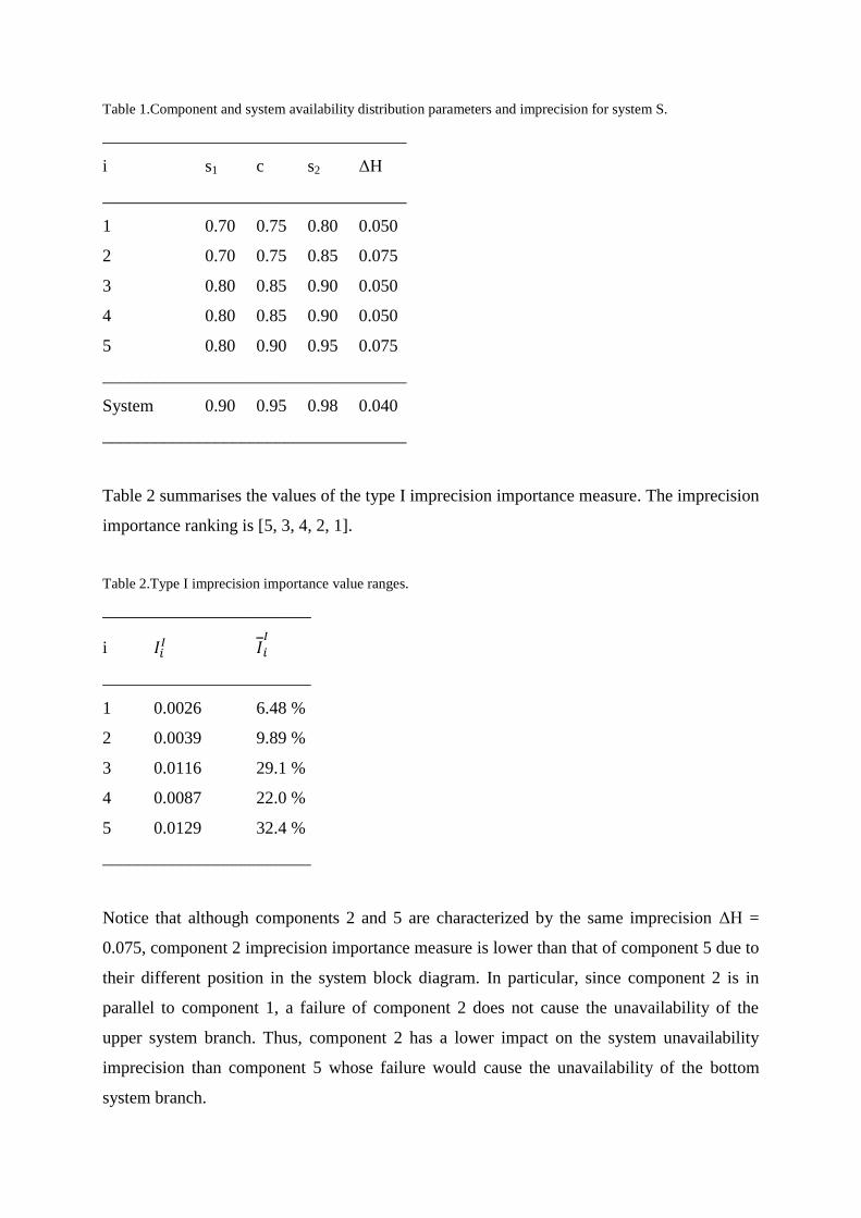
Table 1.Component and system availability distribution parameters and imprecision for system S.
___________________________________
i s1 c s2 ΔH
___________________________________
1 0.70 0.75 0.80 0.050
2 0.70 0.75 0.85 0.075
3 0.80 0.85 0.90 0.050
4 0.80 0.85 0.90 0.050
5 0.80 0.90 0.95 0.075
___________________________________
System 0.90 0.95 0.98 0.040
___________________________________
Table 2 summarises the values of the type I imprecision importance measure. The imprecision
importance ranking is [5, 3, 4, 2, 1].
Table 2.Type I imprecision importance value ranges.
________________________
i
________________________
1 0.0026 6.48 %
2 0.0039 9.89 %
3 0.0116 29.1 %
4 0.0087 22.0 %
5 0.0129 32.4 %
________________________
Notice that although components 2 and 5 are characterized by the same imprecision ΔH =
0.075, component 2 imprecision importance measure is lower than that of component 5 due to
their different position in the system block diagram. In particular, since component 2 is in
parallel to component 1, a failure of component 2 does not cause the unavailability of the
upper system branch. Thus, component 2 has a lower impact on the system unavailability
imprecision than component 5 whose failure would cause the unavailability of the bottom
system branch.

5.2 Type II measure
We now assume that the distributions on thecomponent availabilities and the resulting
distribution on the system availability are asshownin Figure 7.
Figure 7. Input distribution functions on component availabilities and resulting system availability.
Let s1 and s2 (c1 and c2) denote the lower and upper support (core) limits of a possibility
distribution, respectively. For a trapezoidal distribution we have s1< c1< c2< s2, for a
triangular distribution s1< c1 = c2< s2, and for a uniform distribution s1 = c1< c2 = s2. For these
distribution classes we then have that the imprecision equals
(16)

Table 1 lists the possibility distribution parameters and the associated imprecision, at both
component and system level.
Table 3.Component and system availability distribution parameters and imprecision for system S.
_________________________________________
i s1 c1 c2 s2 ΔHq
_________________________________________
1 0.70 0.75 0.75 0.80 0.05
2 0.70 0.75 0.80 0.85 0.10
3 0.80 0.80 0.90 0.90 0.10
4 0.80 0.85 0.85 0.90 0.05
5 0.80 0.85 0.90 0.95 0.10
_________________________________________
System 0.90 0.93 0.97 0.98 0.057
_________________________________________
Figure 8shows the relative variant of the type II imprecision importance measure for all five
components in system S.

Figure 8.Relative variant of the type II imprecision importance measurefor each component insystem S.
The (relative) imprecision importance for each component is evaluated as a function of qi on
the support of the associated distribution. Table 2 summarises the value ranges of the
(R)IRIM. The imprecision importance ranking is [3, 5, 4, 2, 1] according to both high and low
values.
Table 4.Type II imprecision importance value ranges.
______________________________________
i
______________________________________
1 [0.0006, 0.0046] [1.13 %, 8.10 %]
2 [0.0032, 0.0079] [5.60 %, 13.8 %]
3 [0.0182, 0.0294] [31.7 %, 51.2 %]
4 [0.0040, 0.0129] [6.94 %, 22.5 %]
5 [0.0094, 0.0239] [16.4 %, 41.6 %]
______________________________________

Notice that, although components 1 and 2 are in parallel, component 2 is characterized by
larger Type II imprecision importance value ranges than component 1. This is due to the fact
that our knowledge on q2 is more imprecise than that on q1, being ΔH2 = 0.10 whereas ΔH1 =
0.05. Thus, as expected, removing the imprecision on the more imprecise input causes a larger
reduction of the system unavailability imprecision.
6 Discussion and conclusions
In the present paper, we have described and applied an importance measure that can be used
to evaluate the effect on system level parameter imprecision of removing component level
parameter imprecision. Hence, the suggested measure is defined analogously to the classical
improvement potential IM which describes the effect of removing the unreliability of a
component, and analogously with a number of UIMs that describe the effect of removing
uncertainty about component performance.
Two extents of imprecision removal are considered: reduction to a probabilistic representation
(type I) and removal of epistemic uncertainty (type II), the latter a special case of the former.
The relative version of the measure expresses the fraction of the initial amount of imprecision
on the system level parameter that is attributable to each component. In a ranking setting this
format is perhaps easier to comprehend than the underlying absolute numbers; however, the
fractions need to be seen in relation to the initial amount of imprecision on the system level
parameter.
IIMs may be seen as an extension of UIMs when the uncertainty representation is no longer
single-valued probability but instead some alternative representation with the interpretation of
lower and upper probabilities.
An alternative to the measure ofimprecision used in the present paper, and hence relevant for
future work,is the Hartley-like measure of non-specificity, variants of which exist for both
possibility and evidence theory; see Klir (2006; 1999).

Further work in relation to the suggested measure could also be directed towards
implementation of the type II measure on more complex systems. Moreover, possibility
theory provides a relatively simple and hence convenient uncertainty representation to use for
the implementation of the suggested measures; however, other representations couldalso be
considered in terms of application depending on the particular uncertainty setting. Finally,
future work will also be devoted to the investigation of the proposed imprecision uncertainty
importance measures in presence of dependences in the input considered for the analysis.
Acknowledgements
The authors are grateful to two anonymous reviewers for useful comments and suggestions to
an earlier version of the present paper.
The work of T. Aven and R. Flage has been partially funded by The Research Council of
Norway through the PETROMAKS research program. The financial support is gratefully
acknowledged.
The work of E. Zio and P. Baraldi has been partially funded by the “Foundation pour une
Culture de Securite’ Industrielle” of Toulouse, France, under the research contract AO2009-
04.
References
Apostolakis, G.E. 1990. The concept of probability in safety assessments of technological
systems.Science 250(4986): 1359-1364.
Aven, T. & Jensen, U. 1999.Stochastic Models in Reliability. New York: Springer.
Aven, T. &Nøkland, T.E. 2010 On the use of uncertainty importance measures in reliability
and risk analysis. Reliability Engineering and System Safety 95(2): 127-133.
Baraldi, P., Librizzi, M., Zio, E., Podofillini, L. &Dang, V.N. 2009. Two techniques of
sensitivity and uncertainty analysis of fuzzy expert systems. Expert Systems with
Applications 36(10): 12461-12471.
Baraldi, P. &Zio, E. 2008 A combined Monte Carlo and possibilistic approach to uncertainty
propagation in event tree analysis.Risk Analysis 28(5): 1309-1325.
Baudrit, C., Dubois D. &Guyonnet D. 2006.Joint propagation of probabilistic and possibilistic
information in risk assessment.IEEE Transactions on Fuzzy Systems 14(5): 593-608.
Berger, J.O. 1984 The robust Bayesian viewpoint. In J. B. Kadane, JB (ed.), Robustness of
Bayesian Analyses: 63-144. Amsterdam: Elsevier Science.
Borgonovo, E. 2006.Measuring uncertainty importance: Investigation and comparison of
alternative approaches.Risk Analysis 26(5): 1349-1361.
Dempster, A.P. (1967) Upper and lower probabilities induced by a multivalued mapping. The
Annals of Mathematical Statistics 38: 325-339.
Dubois, D. 2006. Possibility theory and statistical reasoning.Computational Statistics & Data
Analysis 51: 47-69.
Dubois, D. &Prade, H. (1992)When upper probabilities are possibility measures. Fuzzy Sets
and Systems 49: 65-74.
Dubois, D., Prade H. &Sandri S. 1993. On possibility/probability transformations. In: Lowen
R, Roubens M, editors. Fuzzy Logic: State of the Art. Dordrecht: Kluwer Academic
Publishers. pp. 103–112.
Cheok, M.C., Parry, G.W. and Sherry, R.R. 1998. Use of importance measures in risk-
informed regulatory applications.Reliability Engineering and System Safety 60: 213-226.
Dubois, D. &Prade, H. 1988.Possibility Theory – An Approach to Computerized Processing
of Uncertainty. New York: Plenum Press.

Ferson, S., Kreinovich, V., Ginzburg, L., Myers, D.S. &Sentz, K. 2003.Constructing
probability boxes and Dempster-Shafer structures.Technical Report SAND2002-4015, Sandia
National Laboratories.
Flage, R., Baraldi, P., Zio, E.& Aven, T. (2011) On imprecision in relation to uncertainty
importance measures. In: Bérenguer, C., Grall, A.&GuedesSoares, C. (eds) Advances in
Safety, Reliability and Risk Management. Proceedings of the European Safety and Reliability
Conference (ESREL) 2011, Troyes, France, 18-22 September 2011. pp. 2250-2255.
Helton, J C &Burmaster, D E (1996) Guest editorial: treatment of aleatory and epistemic
uncertainty in performance assessments for complex systems. Reliability Engineering and
System Safety 54: 91-94.
Iman, R.L. 1987. A matrix-based approach to uncertainty and sensitivity analysis for fault
trees. Risk Analysis 7(1): 21-33.
Kalos M.H. & Whitlock P.A. 1986.Monte Carlo Methods. Volume I: Basics. Wiley.
Kaplan, S. & Garrick, B.J. 1981.On the quantitative definition of risk.Risk Analysis 1(1): 11-
27.
Klir, G.J. (2006) Uncertainty and Information: Foundations of Generalized Information
Theory. Hoboken, N.J.: Wiley-Interscience.
Klir, G.J. (1999) Uncertainty and Information Measures for ImpreciseProbabilities: An
Overview. In: De Cooman, G.,Cozman, F.G., Moral, S. &Walley, P. (eds)ISIPTA
'99.Proceedings of the First International Symposium on Imprecise Probabilities and Their
Applications, Ghent, Belgium, 29 June - 2 July 1999. pp. 234-240.
Pedroni, N. & Zio, E. 2012. Empirical comparison of methods for the hierarchical propagation of
hybrid uncertainty in risk assessment in presence of dependences, International Journal of
Uncertainty, Fuzziness and Knowledge-Based Systems. 20(4):509−557.

Rausand, M. &Høyland, A. 2004. System Reliability Theory: Models, Statistical Methods, and
Applications. 2nd ed. Hoboken, N.J.: Wiley-Interscience.
Shafer, G. 1976. A Mathematical Theory of Evidence.Princeton University Press.
Suresh, P. V., Babar, A. K., & Raj, V. V. (1996). Uncertainty in fault tree analysis: A fuzzy
approach. Fuzzy Sets and Systems, 83, 135–141.
Walley, P. 1991. Statistical Reasoning with Imprecise Probabilities. London: Chapman and
Hall.
Weichselberger, K. 2000. The theory of interval probability as a unifying concept for
uncertainty.International Journal of Approximate Reasoning 24: 149-170.
Zadeh L.A. 1965. Fuzzy sets. Information and Control 8: 338-353.
Zio, E. 2009.Computational Methods for Reliability and Risk Analysis. Hackensack, N.J.:
World Scientific.
Liping, H. & Fuzheng, Q. 2009. Possibilistic entropy-based measure of importance in fault
tree analysis. Journal of Systems Engineering and Electronics 20(2): 434-444.


![Uncertainty analysis in the unavailability assessment ...analysis based on fuzzy logic and fuzzy set theory are a kind of representation of the imprecision for complex system. [6]](https://img.pdfslide.net/doc/110x75/5f419ed70ef83e0ea447c440/uncertainty-analysis-in-the-unavailability-assessment-analysis-based-on-fuzzy.jpg)