AN IMPROVED ALGORITHM FOR CHANNEL ALLOCATION ON DIRECT SEQUENCE SPREAD SPECTRUM

HANDRIZAL

Thesis submitted in fulfillment of the requirements For the award of the degree of Master of Science in Computer

Faculty of Computer Systems & Software Engineering UNIVERSITI MALAYSIA PAHANG

JULY 2011

iv

ABSTRACT

Graph coloring is an assignment a color to each vertex, which each vertex that adjacent is given a different color. Graph coloring is a useful algorithm for channel allocation on Direct Sequence Spread Spectrum (DSSS). Through this algorithm, each access point (AP) that adjacent gives different channels based on colors available. Welsh Powell algorithm and Degree of saturation (Dsatur) are the popular algorithms being used for channel allocation in this domain. Welsh Powell algorithm is an algorithm that tries to solve the graph coloring problem. Dsatur algorithm is an algorithm coloring sorted by building sequence of vertices dynamically. However, these algorithms have its weaknesses in terms of the minimum number of channel required. In this study, channel allocation called Vertex Merge Algorithm (VMA) is proposed with aim to minimize number of required channels. It is based on the logical structure of vertex in order to a coloring the graph. Each vertex on the graph arranged based on decreasing number of degree. The vertex in the first place on the set gives a color, and then this vertex is merged with non-adjacent vertex. This process is repeatedly until all vertices colored. The assignment provides a minimum number of channels required. A series of an experiment was carried out by using one computer. Vertex Merge Algorithm (VMA) simulation is developed under Linux platform. It was carried out in Hypertext Preprocessor (PHP) programming integrated with GNU Image Manupulation Program (GIMP) for open and edit image. The experimental results show that the proposed algorithm work successfully in channel allocation on DSSS with the minimum of channels required. The average percentage reduction in the number of required channels among the VMA, Dsatur algorithm and Welsh Powell algorithm in the simple graph is equivalent to 0.0%. Meanwhile between the VMA and Dsatur algorithm in the complex graph is equivalent to 18.1%. However, VMA and Welsh Powell algorithm is not compared in the complex graph since its drawback in terms of not fulfill the graph coloring concept. This is because there are two adjacent vertices have the same color. Overall, even there is no reduction for number of required channel among VMA, Dsatur algorithm and Welsh Powell algorithm in the simple graph, but the outstanding significant contribution of VMA since it has reduction in the complex graph.

v

ABSTRAK

Pewarnaan graf merupakan pemberian warna untuk setiap verteks, untuk verteks yang berdekatan diberikan warna yang berbeza. Pewarnaan graf merupakan suatu algoritma yang digunakan bagi penempatan saluran pada Direct Sequence Spread Spectrum (DSSS). Melalui algoritma ini, setiap akses point (AP) yang berdekatan diberikan saluran yang berbeza berdasarkan warna tertentu. Algoritma Welsh Powell dan algoritma Darjah Kejenuhan (Dsatur) merupakan algoritma-algoritma terkenal yang telah digunakan untuk penempatan saluran dalam bidang ini. Algoritma Welsh Powell merupakan algoritma yang cuba menyeselaikan masalah pewarnaan graf. Algoritma Dsatur adalah algoritma pewarnaan graf yang dibuat dengan urutan verteks secara dinamik. Walaubagaimanapun, algoritma-algoritma ini mempunyai kelemahan dari segi jumlah minimum saluran yang diperlukan. Dalam kajian ini, dicadangkan penempatan saluran yang dikenali sebagai Algoritma Vertex Gabung (VMA) dengan tujuan untuk meminimumkan jumlah saluran yang diperlukan. Hal ini berdasarkan susunan logikal verteks untuk membentuk pewarnaan suatu graf dalam penempatan saluran. Setiap verteks dalam graf disusun berdasarkan penurunan jumah darjah. Verteks dalam turutan pertama suatu set diberikan warna, kemudian verteks tersebut digabungkan dengan verteks yang tidak berdekatan. Proses ini terus berulang sehingga kesemua verteks diberikan warna. Ketetapan ini telah menyediakan jumlah saluran minimum yang diperlukan. Suatu siri eksperimen telah dijalankan dengan menggunakan sebuah komputer. Simulasi Algoritma Verteks Gabung (VMA) telah dibangunkan di bawah platfom Linux. Ia telah dibina dengan bahasa pengaturcaraan Prapemroses Hiperteks (PHP) serta berintegrasikan GNU Image Manipulation Program (GIMP) untuk memaparkan dan mengemaskinikan gambar. Keputusan eksperimen menunjukkan bahawa algoritma yang dicadangkan telah berjaya dalam penempatan saluran pada Direct Sequence Spread Spectrum (DSSS) dengan jumlah saluran minimum yang diperlukan. Purata peratusan penurunan jumlah saluran di antara VMA, Dsatur algoritma dan Welsh Powell algoritma dalam graf sederhana adalah bersamaan dengan 0.0%. Sementara itu, di antara VMA dan Dsatur algoritma dalam graf kompleks adalah bersamaan dengan 18.1%. Namun, VMA dan Welsh Powell algoritma tidak dibandingkan dalam kompleks graf disebabkan kelemahan dalam hal tidak memenuhi konsep pewarnaan graf. Hal ini disebabkan terdapat dua verteks bersebelahan memiliki warna yang sama. Secara keseluruhan, tidak ada penurunan jumlah saluran yang diperlukan antara VMA, Dsatur algoritma dan Welsh Powell algoritma di dalam graf sederhana. Walaubagaimanapun, sumbangan penting VMA adalah penurunan jumlah saluran yang diperlukan di dalam kompleks graf.

vi

TABLE OF CONTENTS

Page

SUPERVISOR’S DECLARATION i

STUDENT’S DECLARATION ii

ACKNOWLEDGMENT iii

ABSTRACT iv

ABSTRAK v

TABLE OF CONTENTS vi

LIST OF TABLES ix

LIST OF FIGURES xi

LIST OF SYMBOLS xiii

LIST OF ABBREVIATIONS xiv

CHAPTER 1 INTRODUCTION

1.1 Introduction 1

1.2 Channel Allocation 2

1.3 Problem Statement 3

1.4 Research Objectives 5

1.5 Research Scope 5

1.6 Organization of Thesis 5

1.7 Conclusion 5

CHAPTER 2 FUNDAMENTAL CONCEPTS AND THEORY

2.1 Introduction 7

2.2 Direct Sequence Spread Spectrum (DSSS) 7

2.2.1 Channel 8

2.3 Definition of Graph 10

2.4 Common Families of Graphs 13

2.4.1 Simple Graph 13 2.4.2 Complete Graph 14

vii

2.4.3 Bipartite Graph 14 2.4.4 Complement Graph 15 2.4.5 Complex Graph 17

2.5 Graph Operations 17

2.6 Graph Coloring 18

2.6.1 Chromatic Numbers for Common Graph Families 19

2.7 Welsh Powell Algorithm 22

2.7.1 An Example of Welsh Powell Algorithm 22

2.8 Degree of Saturation Algorithm 26

2.8.1 An Example of Dsatur Algorithm 27

2.9 Research Methodology 33

2.10 Conclusion 34

CHAPTER 3 VERTEX MERGE ALGORITHM

3.1 Introduction 36

3.2 Vertex Merge Algorithm 36

3.3 VMA in Channel Allocation 39

3.3.1 Interference Graphs 39

3.4 An Example of VMA 41

3.5 Conclusion 47

CHAPTER 4 EXPERIMENT AND RESULT ANALYSIS

4.1 Introduction 49

4.2 Hardware and Software Specification 49

4.3 Experiment 50

4.3.1 Coloring of Channel 54 4.3.2 Create VMA, Dsatur and Welsh Powell Script 55 4.3.3 A Simulation Example 56

4.4 Results and Discussion 66

4.4.1 Case 1: Simple Graph 67 4.4.2 Case 2: Complex Graph 74

4.5 Conclusion 85

viii

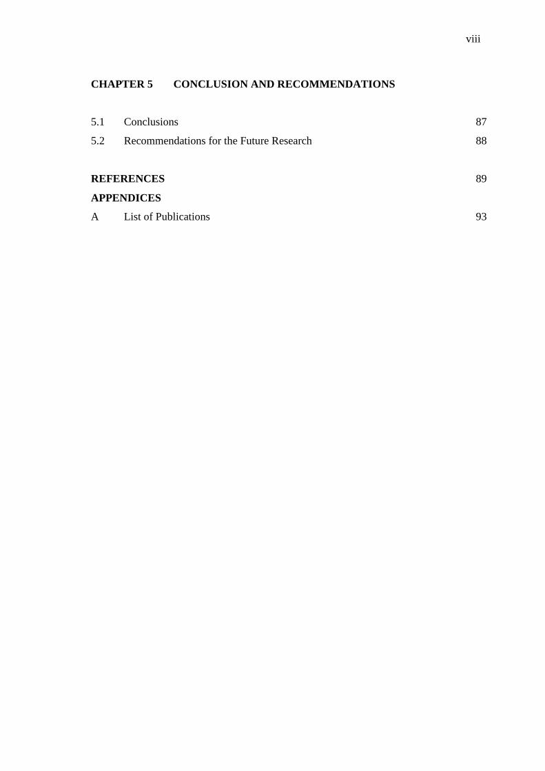
CHAPTER 5 CONCLUSION AND RECOMMENDATIONS

5.1 Conclusions 87

5.2 Recommendations for the Future Research 88

REFERENCES 89

APPENDICES

A List of Publications 93

ix

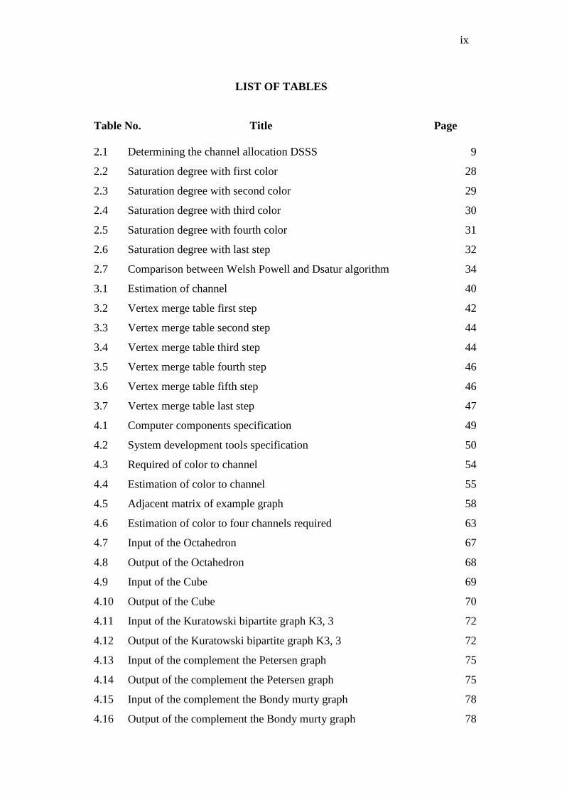
LIST OF TABLES

Table No. Title Page 2.1 Determining the channel allocation DSSS 9

2.2 Saturation degree with first color 28

2.3 Saturation degree with second color 29

2.4 Saturation degree with third color 30

2.5 Saturation degree with fourth color 31

2.6 Saturation degree with last step 32

2.7 Comparison between Welsh Powell and Dsatur algorithm 34

3.1 Estimation of channel 40

3.2 Vertex merge table first step 42

3.3 Vertex merge table second step 44

3.4 Vertex merge table third step 44

3.5 Vertex merge table fourth step 46

3.6 Vertex merge table fifth step 46

3.7 Vertex merge table last step 47

4.1 Computer components specification 49

4.2 System development tools specification 50

4.3 Required of color to channel 54

4.4 Estimation of color to channel 55

4.5 Adjacent matrix of example graph 58

4.6 Estimation of color to four channels required 63

4.7 Input of the Octahedron 67

4.8 Output of the Octahedron 68

4.9 Input of the Cube 69

4.10 Output of the Cube 70

4.11 Input of the Kuratowski bipartite graph K3, 3 72

4.12 Output of the Kuratowski bipartite graph K3, 3 72

4.13 Input of the complement the Petersen graph 75

4.14 Output of the complement the Petersen graph 75

4.15 Input of the complement the Bondy murty graph 78

4.16 Output of the complement the Bondy murty graph 78

x

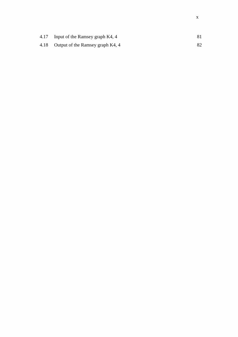
4.17 Input of the Ramsey graph K4, 4 81

4.18 Output of the Ramsey graph K4, 4 82

xi

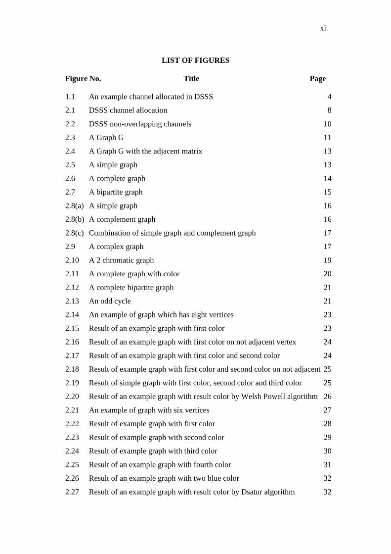
LIST OF FIGURES Figure No. Title Page

1.1 An example channel allocated in DSSS 4

2.1 DSSS channel allocation 8

2.2 DSSS non-overlapping channels 10

2.3 A Graph G 11

2.4 A Graph G with the adjacent matrix 13

2.5 A simple graph 13

2.6 A complete graph 14

2.7 A bipartite graph 15

2.8(a) A simple graph 16

2.8(b) A complement graph 16

2.8(c) Combination of simple graph and complement graph 17

2.9 A complex graph 17

2.10 A 2 chromatic graph 19

2.11 A complete graph with color 20

2.12 A complete bipartite graph 21

2.13 An odd cycle 21

2.14 An example of graph which has eight vertices 23

2.15 Result of an example graph with first color 23

2.16 Result of an example graph with first color on not adjacent vertex 24

2.17 Result of an example graph with first color and second color 24

2.18 Result of example graph with first color and second color on not adjacent 25

2.19 Result of simple graph with first color, second color and third color 25

2.20 Result of an example graph with result color by Welsh Powell algorithm 26

2.21 An example of graph with six vertices 27

2.22 Result of example graph with first color 28

2.23 Result of example graph with second color 29

2.24 Result of example graph with third color 30

2.25 Result of an example graph with fourth color 31

2.26 Result of an example graph with two blue color 32

2.27 Result of an example graph with result color by Dsatur algorithm 32

xii

Figure No. Title Page

2.28 Flowchart of methodology research 33

3.1 An example of graph 42

3.2 An example of graph with first step VMA 43

3.3 An example of graph with second step VMA 43

3.4 An example of graph with third step VMA 44

3.5 An example of graph with fourth step VMA 45

3.6 An example of graph with fifth step VMA 45

3.7 An example of graph with sixth step VMA 46

3.8 An example of graph with last step VMA 47

4.1 Flowchart of Welsh Powell algorithm 51

4.2 Flowchart of Dsatur algorithm 52

4.3 Flowchart the proposed algorithm 53

4.4 VMA simulator script 56

4.5 VMA simulator ready to run 57

4.6 An example of graph to input VMA simulator 58

4.7 Open gedit to input data 59

4.8 Input adjacent matrix to gedit 60

4.9 Save file input of VMA simulation with txt format 61

4.10 Input file of VMA simulation has been saved 61

4.11 The input file to VMA simulation 62

4.12 Output of VMA simulation in text format 62

4.13 Input and Output have been included in the folder of VMA 64

4.14 Output of VMA simulation in the graph model 65

4.15 Output of VMA simulation in the graph coloring format 66

4.16 Comparison between VMA, Dsatur and Welsh Powell simulator in

the simple graph 74

4.17 Comparison between VMA and Dsatur simulator in the complex graph 84

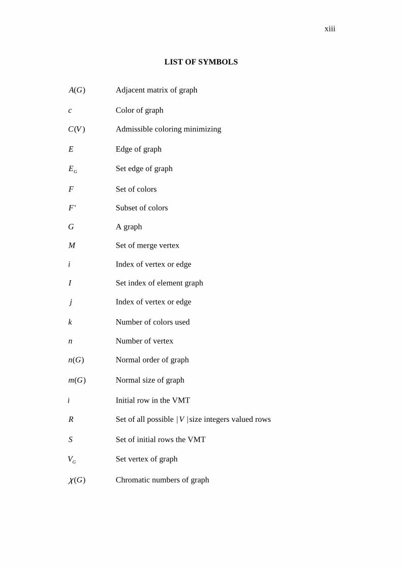
xiii

LIST OF SYMBOLS

)(GA Adjacent matrix of graph c Color of graph

)(VC Admissible coloring minimizing E Edge of graph

GE Set edge of graph

F Set of colors

'F Subset of colors G A graph M Set of merge vertex i Index of vertex or edge I Set index of element graph j Index of vertex or edge

k Number of colors used n Number of vertex

)(Gn Normal order of graph

)(Gm Normal size of graph l Initial row in the VMT R Set of all possible ||V size integers valued rows S Set of initial rows the VMT

GV Set vertex of graph

)(Gχ Chromatic numbers of graph

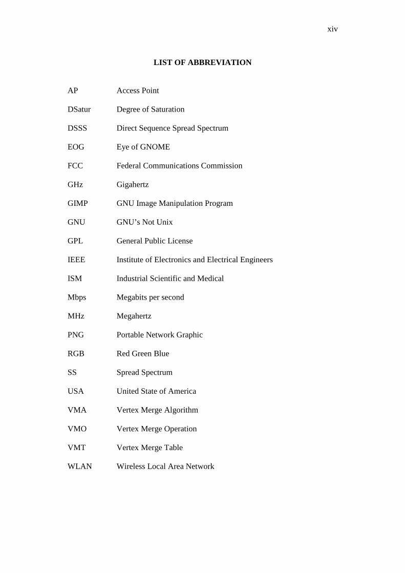
xiv

LIST OF ABBREVIATION

AP Access Point DSatur Degree of Saturation DSSS Direct Sequence Spread Spectrum EOG Eye of GNOME FCC Federal Communications Commission GHz Gigahertz GIMP GNU Image Manipulation Program GNU GNU’s Not Unix GPL General Public License IEEE Institute of Electronics and Electrical Engineers ISM Industrial Scientific and Medical Mbps Megabits per second MHz Megahertz PNG Portable Network Graphic RGB Red Green Blue SS Spread Spectrum USA United State of America VMA Vertex Merge Algorithm VMO Vertex Merge Operation VMT Vertex Merge Table WLAN Wireless Local Area Network

1

CHAPTER 1

INTRODUCTION

1.1 INTRODUCTION

The spectacular development of network and the internet has a big impact to the

companies in various types and sizes. The advanced wireless technologies support the

development of network, the internet and intranet capability for the mobile workers,

isolated area and temporary facilities. Wireless expands and increases the capability of

computer networking. The new technologies enable the wireless networking as one of

the access in higher velocity and qualified for the computer network and the internet.

The wireless networks based on the Institute of Electrical and Electronics

Engineers (IEEE) 802.11 standards (IEEE, 2007). This technology presents important

disadvantages if compared with other radio networks, as a shorter range, security issue,

difficulties providing inter-network or inter-operator roaming. However, the networks

based on the IEEE 802.11 are unquestionably being chosen by most of the users

(Gracia, 2005). Its popularity comes noticeable, beyond the evident advantages of

the radio networks in contrast to the wired networks.

Nowadays, it is a common thing to see the coexistence of many Wireless

Local Area Network (WLAN) networks in densely populated areas, either of

private or of public nature (Hot-Spots), corporative. Domestic users use it to avoid

the installation of new wires in their homes and to communicate with other users,

in offices or university campuses are used to provide access to the internet or

corporative intranets to their employees or students and, lately, operators and

Internet Service Provider (ISP) have found a new market offering this access in

public places, like hotels, airports or convention centers. With a high density of

nodes, the presence of interference increases causing the performance perceived by

users to degrade. In order to reduce the effect of interferences in cellular networks, a

2

channel planning is traditionally used. In cases of 802.11b and 802.11g WLAN

networks, frequency channels are a scarce resource, since we can only count on three

non overlapping channels. Therefore, the Channel Allocation Problem (CAP) is an

important issue to solve.

1.2 CHANNEL ALLOCATION

Channel allocation can be defined as choosing, which channel the access point

should use to communicate with the wireless terminals in its subnet without interfering

with the transmissions from the other’s access points (Mahonen et al. 2004).

Understanding of channel allocation is very important because it relates to the overall

capacity of wireless local area networks (Carpenter, 2008).

Channel allocation in WLAN 802.11 networks is studied as a part on the

design of multicellular WLANs working in infrastructure mode. A good design

can be evaluated according to two basic requirements: full coverage of the

required area and the provision of a capacity suitable to support the traffic that is

generated, without degrading the service as the number of user’s increases. Although

there is an endless list of parameters to consider, the requirements mentioned

above can be obtained with an exhaustive selection of Access Points (APs) locations

and the proper set of channels and power levels.

Several research articles have been published regarding channel allocation.

Among them were those by (Al Mamun et.al. 2009; Chen et.al. 2008; Duan et.al. 2010;

Mahonen et.al. 2004; Malone et.al. 2007; Raj, 2006; Riihijarvi et.al. 2005; 2006;

Yuqing et.al. 2010; Yue et.al. 2010; and Zhuang et.al. 2010) Those articles revealed that

channel allocation for DSSS is one of the current issues that still unsolved in channel

allocation. Therefore, the study on this basis is initiated.

Wireless Local Area Networks (WLANs) operate in unlicensed portions of the

frequency spectrum allotted by a regulatory body, like the Federal Communications

Commission (FCC) in the United States of America (Goldsmith, 2005; IEEE, 2007).

Each WLAN standard (802.11/a/b/g) defines a fixed number of channels for use by

3

access point (AP) and mobile users. For example, the 802.11b/g standard defines a total

of 14 frequency channels of which 1 through 11 are permitted in the United States of

America (Guizani, 2004). Actually, channel represents the center of frequency. There is

only 5 MHz separation between the center frequencies. The signal falls within about 15

MHz of each side of the center frequency. Consequently, an 802.11b/g signal overlaps

with several adjacent channel frequencies. Therefore, only three channels (channels 1,

6, and 11) available for use without causing interference (Gracia, 2005; Rackley, 2007;

Theodore, 2001).

The Wireless LAN standard 802.11b and 802.11g in the process of distributing

data using Direct Sequence Spread Spectrum (DSSS) technology (Goldsmith, 2005).

DSSS works by taking a data stream of zeros and ones and modulating it with a second

pattern, the chipping sequence. Various other electronic devices in a home, such as

cordless phones, garage door openers, and microwave ovens, maybe use same

frequency range. Any such device can interfere with a WLANs network, slowing down

its performance and potentially breaking network connections (Perez, 1998; Theodore,

2001).

1.3 PROBLEM STATEMENT

According to the overview in the Section 1.1, DSSS system only has three none

overlapping channels are located (Rackley, 2007; Theodore, 2001). When more than

three access points (APs) are in same location, it may cause interference with another

AP. Interference in communications is anything, which alters, modifies, or disrupts a

signal as it travels along a channel between a source and a receiver (James, 2008;

Stallings, 2003). In addition, interference decreased the network performance.

Thus, some of the research problems that arise in channel allocation can be

stated as follows:

• How does allocate channel while there is more than three access points in

same location?

• How to reduce the number of channels while there is more than three access

points in same location?

4

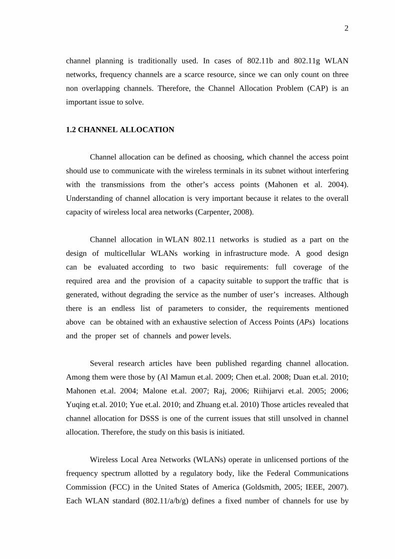
Figure 1.1 shows the channel allocation problem when there exist more than

three access points in the same area.

Figure 1.1: An example channel allocated in DSSS

From Figure 1.1 it can be seen that any interference with each other AP. AP1

interference with AP2, AP3 and AP4. AP2 was interference with AP1, AP3 and AP4. AP3

was interference with AP1, AP2 and AP4. AP4 was interference with AP1, AP2 and AP3.

Every AP is given one channel. Based on DSSS channel allocation, the AP1 given

channel 1, AP2 channel 6, AP3 channel 11 and AP4 another channel. When AP4 is given

channel, there was interference between APs. It leads to degradation overall network

performance.

Currently, the internet is a very fast growth. Installation of AP more than three is

inevitable. One way to solve this problem is minimizing the number of channels used.

Several research articles have been published regarding this problem. Dsatur algorithm

(Brelaz, 1979) and Welsh Powell algorithm (Welsh, 1967) has been proposed to

determine the minimal number of color in the graph coloring theory. Riihijarvi (2006)

enhanced Dsatur algorithm by determining the number of channel, based on the high

degree of saturation access point. Meanwhile, Rohit (2008) enhance the Welsh Powell

algorithm by determining the number of channel, based on high degree of access point.

Both of these algorithms, has worked perfectly to determine the number of required

channels. However, the number of channels is obtained using this algorithm is still

large. Thus, create a new algorithm is motivation in this research to minimize the

number of required channels.

Channel 1

Channel 11 Channel ?

Channel 6

AP1

AP4

AP2

AP3

1

5

1.4 RESEARCH OBJECTIVES

The objectives of the research are as follows:

a) To propose a new algorithm to allocate and reduce the number of required

channels.

b) To test the performances of the proposed algorithm.

1.5 RESEARCH SCOPE

In this research, the following scope has been identified:

a) The new algorithm channel allocated for Direct Sequence Spread Spectrum is

simulated by using the PHP.

b) The simulation results will be compared with the Welsh Powell algorithm

(Rohit, 2008), and Degree of Saturation (DSatur) algorithm (Riihijarvi, 2006).

The Vertex Merge Algorithm (VMA) is proposed based on the graph coloring in

order to reduce the required channel. The motivations of this simulation are to show the

clarity of the algorithm, and provide the VMA simulator in order to minimize number of

required channels.

1.6 ORGANIZATION OF THESIS

This thesis is organized as follows: Chapter 1 presents the background, problem

statement, research objectives, research scope and organization of this thesis. Chapter 2

reviews basic concepts, definitions and theorems in graph theory, wireless technology,

as well as algorithms used in this thesis. Chapter 3 proposes the Vertex Merge

Algorithm (VMA). The experiment and result are elaborated in Chapter 4. Finally, the

conclusion and recommendations for the future research are presented in Chapter 5.

1.7 CONCLUSION

This chapter introduces the channel allocation and Direct Sequence Spread

Spectrum (DSSS) technology. Channel allocation in DSSS is the main focus attention

6

this research has been elaborated. Together with advantages of channel allocation brings

specific problems. It occurs since the bigger number of access points. Determine of

channel mechanisms to reducing the number of required channel become the issues.

Thus suggest that proper strategies are required to solve the problems, which are the

significance of this research.

7

CHAPTER 2

FUNDAMENTAL CONCEPTS AND THEORY

2.1 INTRODUCTION

This chapter describes the fundamental philosophical foundation which is a part

of methodology. The basic concepts of the Direct Sequence Spread Spectrum (DSSS),

channel on direct sequence spread spectrum, graph theory, graph coloring, vertex

coloring and graph coloring in channel allocation are presented in this chapter. This

chapter also reviews some of the foremost graph coloring algorithm namely the Welsh

Powell Algorithm (Rohit, 2008) and Degree of Saturation (Dsatur) (Riihijarvi, 2006).

These algorithms are then compared to the proposed Vertex Merge Algorithm (VMA)

in Chapter 4, in terms of number of channel required. In particular, the reviewed

channel allocation algorithm and proposed channel allocation algorithm are based on

these concepts.

2.2 DIRECT SEQUENCE SPREAD SPECTRUM (DSSS)

An increasingly popular form of communications is known as the Spread

Spectrum (SS). The Spread Spectrum technique was developed initially for military and

intelligence requirements. The essential idea is to spread the information signal over a

wider bandwidth in order to make jamming and interception more difficult. The first

type of spread spectrum developed became known as frequency hopping. A more recent

version is the Direct Sequence Spread Spectrum (DSSS). Both techniques are used in

various wireless data network products. They also find use in other communications

applications, such as cordless telephones (Bensky, 2008).

DSSS is one of the most widely used types of spread spectrum technology,

owing its popularity to its ease of implementation and high data rates (Carpenter, 2008).

Most of the equipment or the Wireless LAN device on the market uses DSSS

8

technology. DSSS is a method for sending data in which sender and recipient system is

both on the set wide frequency is 22 MHz divides the available 83.5 MHz spectrum (in

most countries) into 3 wide-band 22 MHz channels. The Institute of Electronics and

Electrical Engineers (IEEE) 802.11 standard calls for use of the 2.4 GHz ISM band

ranging from 2.400 to 2.497 GHz (Theodore, 2001; Goldsmith, 2005).

IEEE set on the use of DSSS data rates 1 or 2 Mbps in the 2.4 GHz Industrial

Scientific and Medical (ISM) band, under the 802.11 standard. Meanwhile, the 802.11b

standard specified data rate of 5.5 and 11 Mbps. IEEE 802.11b tools that work on 5.5 or

11 Mbps capable of communicating with the tools that 802.11 work on 1 or 2 Mbps

802.11b standard provides for backward compatibility. In 2003, the IEEE 802.11g

standard providing a 54 Mbps data rate using the ISM frequencies. The advantage of

802.11g over 802.11a is that it is backward-compatible with 802.11b (IEEE, 2007).

2.2.1. Channel

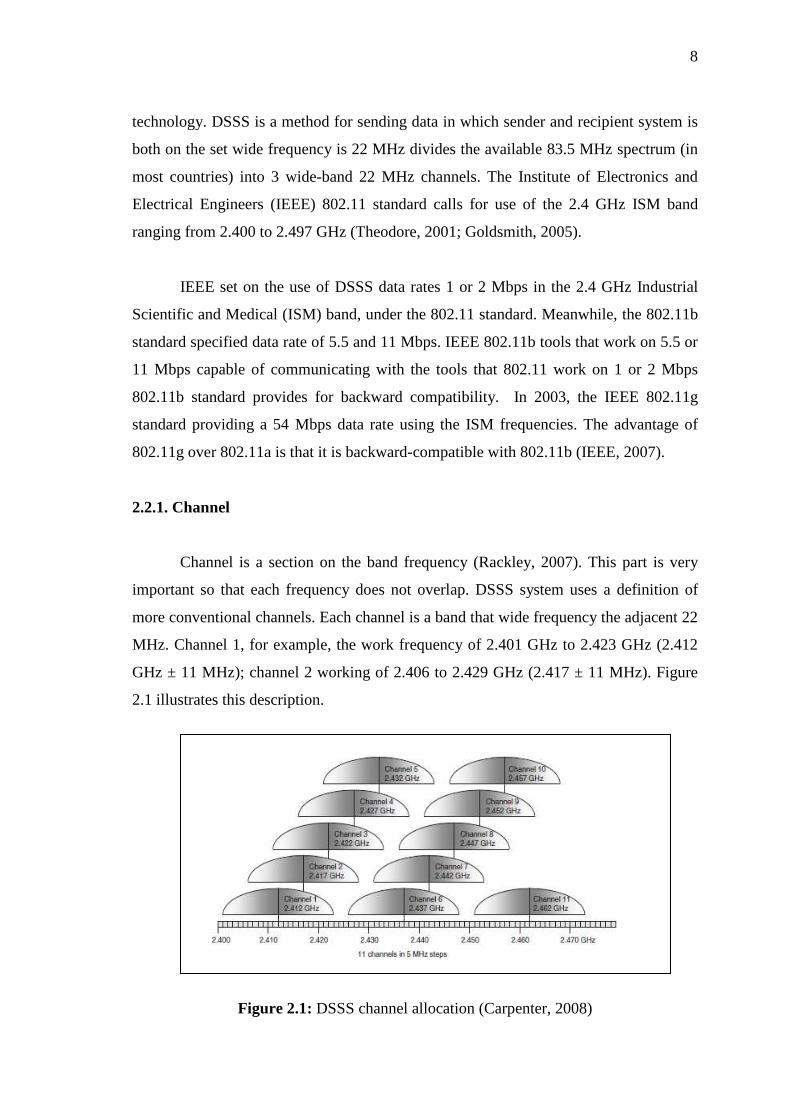
Channel is a section on the band frequency (Rackley, 2007). This part is very

important so that each frequency does not overlap. DSSS system uses a definition of

more conventional channels. Each channel is a band that wide frequency the adjacent 22

MHz. Channel 1, for example, the work frequency of 2.401 GHz to 2.423 GHz (2.412

GHz ± 11 MHz); channel 2 working of 2.406 to 2.429 GHz (2.417 ± 11 MHz). Figure

2.1 illustrates this description.

Figure 2.1: DSSS channel allocation (Carpenter, 2008)

9

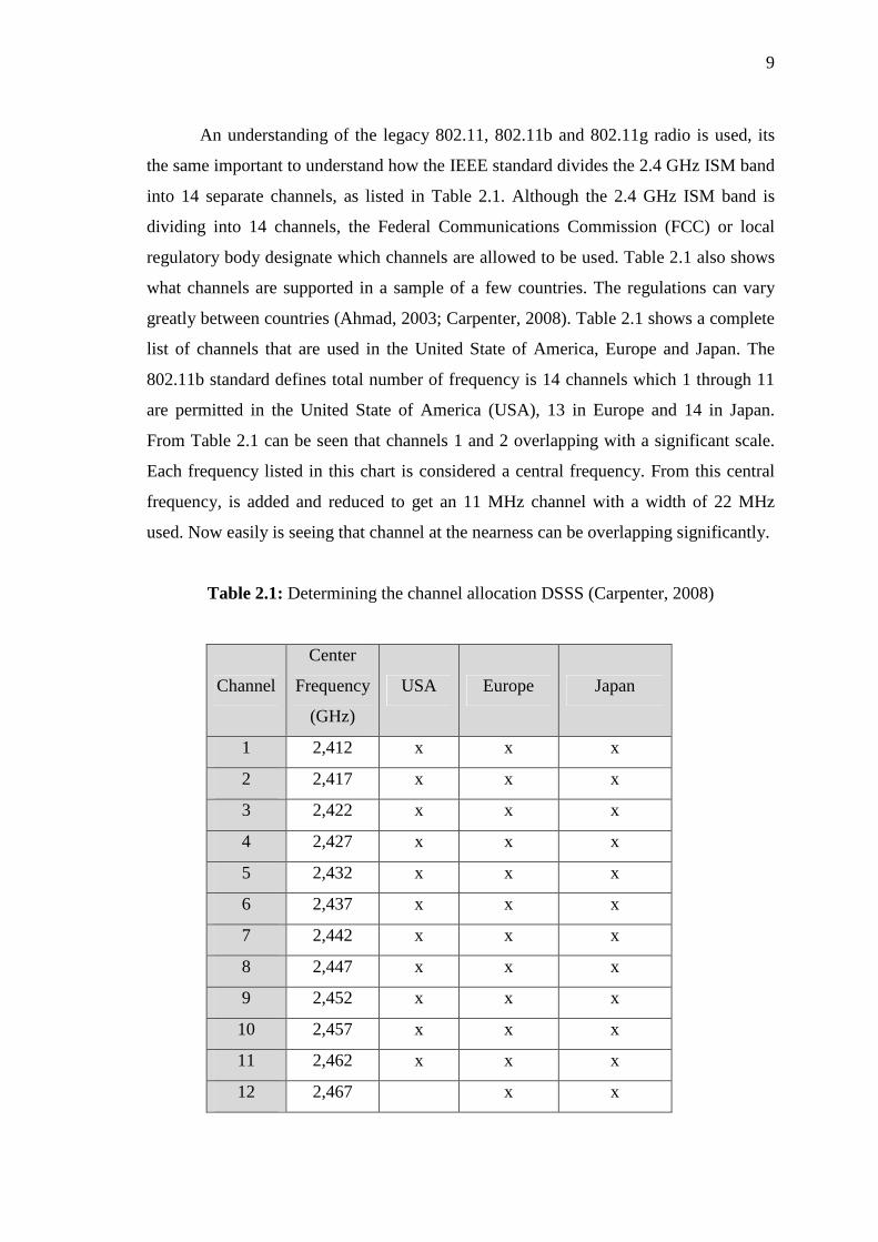
An understanding of the legacy 802.11, 802.11b and 802.11g radio is used, its

the same important to understand how the IEEE standard divides the 2.4 GHz ISM band

into 14 separate channels, as listed in Table 2.1. Although the 2.4 GHz ISM band is

dividing into 14 channels, the Federal Communications Commission (FCC) or local

regulatory body designate which channels are allowed to be used. Table 2.1 also shows

what channels are supported in a sample of a few countries. The regulations can vary

greatly between countries (Ahmad, 2003; Carpenter, 2008). Table 2.1 shows a complete

list of channels that are used in the United State of America, Europe and Japan. The

802.11b standard defines total number of frequency is 14 channels which 1 through 11

are permitted in the United State of America (USA), 13 in Europe and 14 in Japan.

From Table 2.1 can be seen that channels 1 and 2 overlapping with a significant scale.

Each frequency listed in this chart is considered a central frequency. From this central

frequency, is added and reduced to get an 11 MHz channel with a width of 22 MHz

used. Now easily is seeing that channel at the nearness can be overlapping significantly.

Table 2.1: Determining the channel allocation DSSS (Carpenter, 2008)

Channel

Center

Frequency

(GHz)

USA Europe Japan

1 2,412 x x x

2 2,417 x x x

3 2,422 x x x

4 2,427 x x x

5 2,432 x x x

6 2,437 x x x

7 2,442 x x x

8 2,447 x x x

9 2,452 x x x

10 2,457 x x x

11 2,462 x x x

12 2,467 x x

10

13 2,472 x x

14 2,484 x

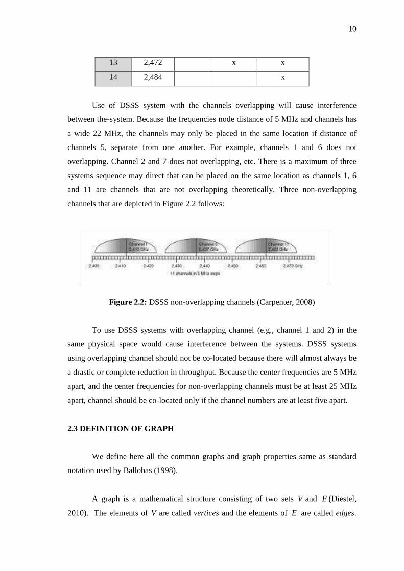
Use of DSSS system with the channels overlapping will cause interference

between the-system. Because the frequencies node distance of 5 MHz and channels has

a wide 22 MHz, the channels may only be placed in the same location if distance of

channels 5, separate from one another. For example, channels 1 and 6 does not

overlapping. Channel 2 and 7 does not overlapping, etc. There is a maximum of three

systems sequence may direct that can be placed on the same location as channels 1, 6

and 11 are channels that are not overlapping theoretically. Three non-overlapping

channels that are depicted in Figure 2.2 follows:

Figure 2.2: DSSS non-overlapping channels (Carpenter, 2008)

To use DSSS systems with overlapping channel (e.g., channel 1 and 2) in the

same physical space would cause interference between the systems. DSSS systems

using overlapping channel should not be co-located because there will almost always be

a drastic or complete reduction in throughput. Because the center frequencies are 5 MHz

apart, and the center frequencies for non-overlapping channels must be at least 25 MHz

apart, channel should be co-located only if the channel numbers are at least five apart.

2.3 DEFINITION OF GRAPH

We define here all the common graphs and graph properties same as standard

notation used by Ballobas (1998).

A graph is a mathematical structure consisting of two sets V and E (Diestel,

2010). The elements of V are called vertices and the elements of E are called edges.

11

Each edge is identified with a pair of vertices. If the edges of the graph G are identified

with ordered pairs of vertices, then G is called a directed graph. Otherwise G it is

called an undirected graph (Koster, 2010). Our discussions in this thesis are concerned

with undirected graphs.

We use the symbols ,...,, 321 vvv to represent the vertices and the symbols

,...,, 321 eee to represent the edges of a graph. The vertices iv and jv associated with and

edge ie are called the end vertices of ie . The edge ie is then denoted as jivve =1 . Note

that while the elements of E are distinct, more than one edge in E may have the same

pair of end vertices. All edges having the same pair of end vertices are called parallel or

multiple edges. Further, the end vertices of an edge need not be distinct. If jivve =1 , then

the edge e1 is called a self-loop at the vertexiv .

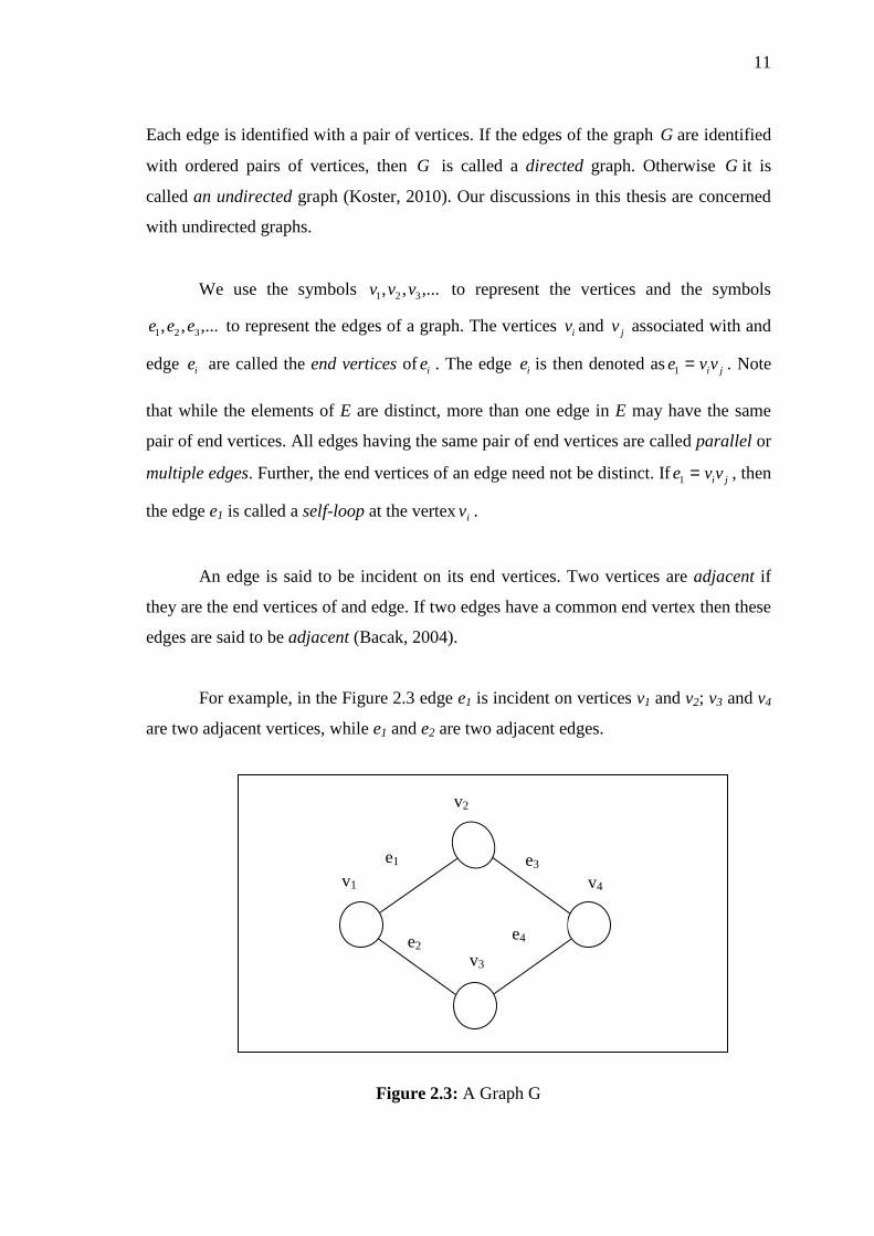
An edge is said to be incident on its end vertices. Two vertices are adjacent if

they are the end vertices of and edge. If two edges have a common end vertex then these

edges are said to be adjacent (Bacak, 2004).

For example, in the Figure 2.3 edge e1 is incident on vertices v1 and v2; v3 and v4

are two adjacent vertices, while e1 and e2 are two adjacent edges.

Figure 2.3: A Graph G

v4 e3

v1

v2

v3

e1

e2 e4

12

The cardinality of the vertex set of a graph G is called the order of G and is

commonly denoted by )(Gn , or more simply by n when the graph under considerations

is clear. Meanwhile, the cardinality of its edge set is the size of G and is often denoted

by )(Gm or m. An (n, m) graph has ordered n and size m. A graph with no edges is

called an empty graph. A graph with no vertex is called a null graph. A subgraph of a

graph G is a graph whose vertex set is a subset of that of G, and whose adjacency

relation is a subset of that of G restricted to this subset.

The number of edge incident on a vertex vi is called the degree of the vertex, and

it is denoted by )deg( iv . Sometimes the degree of a vertex is also referred to as its

valence. By definition, a self-loop at a vertex iv contributes 2 to the degree ofiv . A

vertex is called even or odd according to whether its degree is even or odd. A vertex of

degree 0 in G is called isolated vertex and a vertex of degree 1 is an end-vertex of G.

The minimum degree of G is the minimum degree among the vertices of G and is

denoted by )(Gδ . The maximum degree is defined similarly and is denoted by )(G∆ .

Theorem 2.1 (Euler): The sum of the degrees of a graph is twice the number of edges.

Corollary 2.1: In a graph, there is an even number of vertices having an odd degree.

Proof: Consider separately, the sum of the degrees that are odd and the sum of those

that are even. The combined sum is even by the previous theorem, and since the sum of

the even degrees is even, the sum of the odd degrees must also be an even. Hence, there

must be even number of vertices of odd degree.

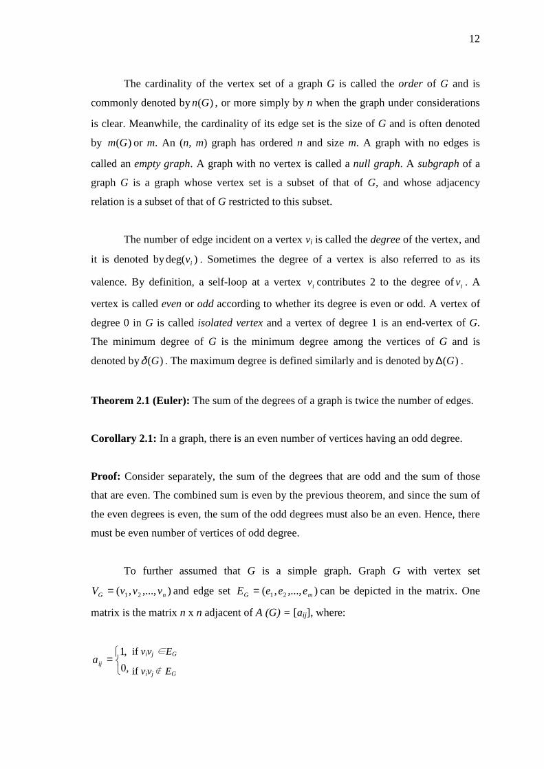
To further assumed that G is a simple graph. Graph G with vertex set

),...,,( 21 nG vvvV = and edge set ),...,,( 21 mG eeeE = can be depicted in the matrix. One

matrix is the matrix n x n adjacent of A (G) = [aij], where:

=,0

,1ija

if vivj EG

if vivj EG

13

Figure 2.4 shows the adjacent matrix of graph G from Figure 2.3

Figure 2.4: A Graph G with the adjacent matrix

2.4 COMMON FAMILIES OF GRAPHS

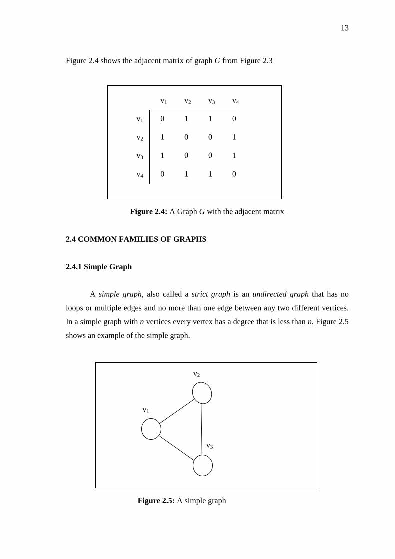
2.4.1 Simple Graph

A simple graph, also called a strict graph is an undirected graph that has no

loops or multiple edges and no more than one edge between any two different vertices.

In a simple graph with n vertices every vertex has a degree that is less than n. Figure 2.5

shows an example of the simple graph.

Figure 2.5: A simple graph

v1 v2 v3 v4

v1 0 1 1 0 v2 1 0 0 1 v3 1 0 0 1 v4 0 1 1 0

v1

v2

v3