An Improved Beam Formulation for Aeroelastic Applications · An Improved Beam Formulation for Aeroelastic Applications ... structural and aerodynamic ﬁelds is performed via the

51st AIAA/ASME/ASCE/AHS/ASC Structures, Structural Dynamics, and Materials Conference, 12–15 April 2010, Orlando, Florida

An Improved Beam Formulation for Aeroelastic

Applications

Alberto Varello∗

Politecnico di Torino, Torino, Italy

San Diego State University, San Diego, CA 92182-1308

Luciano Demasi†

San Diego State University, San Diego, CA 92182-1308

Erasmo Carrera‡

Politecnico di Torino, Torino, Italy

Gaetano Giunta§

Centre de Recherche Public Henri Tudor, Luxembourg-Kirchberg, Luxembourg

A refined beam model for the linear static aeroelastic analysis of generally orientedlifting systems is described in this paper. It is aimed at beam-like structures such as clas-sical and unconventional wing configurations. The structural formulation of refined beamfinite elements is embedded in the framework of Carrera Unified Formulation. Increasingaccuracy in predicting effects of warping, in-plane deformation is obtained by consideringas a free parameter the order of the displacement field expansion over the cross-section.Linear steady aerodynamic loads are described via the Vortex Lattice Method and thetransfer to their energetically equivalent structural loads is performed by the Principleof Virtual Displacements. Thanks to the accuracy of refined elements, the coupling ofstructural and aerodynamic fields is performed via the Infinite Plate Spline method. Theprocedure involves a set of pseudo-structural points placed on the reference surface of thewing system. Different beam elements as well as different higher-order models are consid-ered for the analysis of various cross-section geometries and loading cases. The structuralresults are validated with benchmarks retrieved from the classical models and MSC Nas-tran. Aeroelastic results show well agreement with MSC Nastran solution for a numberof wing configurations. The proposed higher-order model proves its increasing accuracy inpredicting aeroelastic responses with respect to analyses based on classical beam theories.

I. Introduction

IN recent years a push towards the design optimization, aerodynamic and structural understanding of un-conventional wing configurations such as Joined Wings and C-Wings has occurred. Although they have

been examined thoroughly for almost the last 30 years,1−3 their aeroelastic behavior and effect on designare still not completely comprehended.4

Such a kind of wing systems finds applications extending from civil transport to military field. Forinstance, the development of Unmanned Aerial Vehicles (UAVs) has led to the birth of the “sensorcraft”.Sensorcraft is a joined wing aircraft designed for long-range, high-altitude intelligence, surveillance and re-connaissance. Whereas, as far as the box plane is concerned, a study based on PrandtlPlane concept for

∗PhD student, Aeronautics and Space Engineering Department, Politecnico di Torino. Visiting scholar, Department ofAerospace Engineering and Engineering Mechanics, San Diego State University. Student Member AIAA.

†Assistant Professor, Department of Aerospace Engineering and Engineering Mechanics, Member AIAA.‡Professor, Aeronautics and Space Engineering Department, Member AIAA.§Research Scientist, Department of Advanced Materials and Structures, Member AIAA.Copyright c⃝ 2010 by American Institute of Aeronautics and Astronautics, Inc.. Published by the American Institute of

Aeronautics and Astronautics, Inc. with permission.

1 of 23

American Institute of Aeronautics and Astronautics Paper 2010-3032

a 250-300 seat civil transport aircraft was completed for Airbus Deutschland in 2007. Then a static modelof PrandtlPlane designed for Bauhaus Luftfahrt was presented during the Berlin Air Show in May 2008.Again, aeroelastic investigations of geometrically nonlinear lifting surfaces in the past few years coveredhigh-aspect ratio wings of High-Altitude Long-Endurance aircraft5,6 (HALE), strut-braced wings,7,8 truss-braced wings,9 wind tunnel models of delta, beam-like wings and C-Wing configurations.10

Practically, beam-like structures can be analyzed by means of beam theories. Hodges11 developed arelevant example of geometrically exact structural beam model for the dynamics of beam-like structures.However, higher-order beam elements are required in engineering fields such as aeroelasticity where theproper analysis of torsional and bending vibration modes is fundamental to predict aeroelastic responses aswell as critical phenomena. Refined theories are necessary to cope with unconventional cross-section geome-tries, short beams, orthotropic materials and non-homogenous sections.

A review of several beam and plate theories for vibration, wave propagations, buckling and post-bucklingwas presented by Kapania and Raciti.12,13 Particular attention was given to models that account for trans-verse shear-deformation. Moreover, a review about the developments in finite element formulations for thinand thick laminated beams was provided. Kim and White14 investigated non-classical effects in compositebox beam models, such as torsional warping and transverse shear effects. Third-order, locking free beam ele-ment was developed by Reddy,15 where Euler-Bernoulli’s and Timoshenko’s models were obtained as specialcases of the proposed element. Lee16 studied the flexural-torsional behavior of I-shaped composite beams.Transverse shear deformation, coupling and warping effects were accounted for.

Refined theories are also developed by exploiting the asymptotic method. A suitable kinematics modelfor a structural problem is obtained by investigating the role played by the various variables in terms ofa perturbation parameter (usually a geometrical one such as the span-to-height ratio for beams). The 3Dproblem is then reduced to a 1D model by utilizing an asymptotic series of a characteristic parameter andretaining those terms which exhibit the same order of magnitude when the perturbation parameter vanishes.Relevant contributions in developing higher-order beam theories via asymptotic methods are represented byVABS.17−19

In this paper the aeroelastic and structural formulations of refined beam finite elements are addressed.The proposed structural formulation is embedded in the framework of Carrera Unified Formulation (CUF).29

CUF offers a systematic procedure to obtain refined structural models by considering the order of the theoryas a free parameter of the formulation. Different beam elements (with 2, 3 and 4 nodes) as well as differenthigher-order models for the cross-section displacements field are used. Euler-Bernoulli’s and Timoshenko’sbeam models are obtained as particular cases of the first-order formulation. The beam cross-section hasbeen considered rectangular or square and the material is isotropic. The structural results are validatedwith benchmarks retrieved from the classical models and NASTRAN. The proposed aeroelastic formulationis based on the work of Demasi and Livne.10,32 The aeroelastic assessment consists in the comparison ofresults with NASTRAN for several straight and swept wings.

II. Preliminaries

A beam is a structure whose axial extension l is predominant respect to any other dimension orthogonal toit. By intersecting the beam with a plane perpendicular to its axis the beam’s cross-section Ω is identified, asshown in Fig. 1. The Cartesian coordinate system is composed of x and z axes parallel to the cross-sectionplane, whereas the y direction outreaches along the beam axis and is bounded so that 0 ≤ y ≤ l. In general,the origin O can lie outside the contour of the cross-section, which is considered to be constant along thebeam axis identified by the y coordinate. The notation for the displacement vector is:

u(x, y, z

)=

ux uy uz

T

(1)

The stress and strain vectors are split into the terms on the cross-section:

σn =σzy σxy σyy

T

εn =εzy εxy εyy

T

(2)

and the terms lying on planes orthogonal to the cross-section:

σp =σzz σxx σzx

T

εp =εzz εxx εzx

T

(3)

2 of 23


Origin within the cross-section Origin outside the cross-section

Figure 1. Beam’s cross-section geometry and coordinate system.

In the case of small displacement with respect to a characteristic dimension of the cross-section Ω, thefollowing linear relations between strain and displacement components hold:

εn =uz,y + uy,z ux,y + uy,x uy,y

T

εp =uz,z ux,x uz,x + ux,z

T

(4)

The subscripts x, y and z preceded by comma represent the derivatives with respect to the spatial coordinates.A compact vectorial notation can be adopted:

εn = Dnp u + Dny u

εp = Dp u(5)

where Dnp, Dny, and Dp are differential matrix operators:

Dnp =

0

∂

∂z0

0∂

∂x0

0 0 0

, Dny =

0 0∂

∂y

∂

∂y0 0

0∂

∂y0

, Dp =

0 0

∂

∂z

∂

∂x0 0

∂

∂z0

∂

∂x

(6)

In the case of beams made of linear elastic orthotropic materials, the generalized Hooke’s law holds:

σ = C ε (7)

According to Eqs. 2 and 3, the previous expression becomes:

σp = Cpp εp + Cpn εn

σn = Cnp εp + Cnn εn(8)

where matrices Cpp, Cpn, Cnp and Cnn are:

Cpp =

C11 C12 C16

C12 C22 C26

C16 C26 C66

, Cpn = CT

np =

0 0 C13

0 0 C23

0 0 C36

, Cnn =

C55 C45 0

C45 C44 0

0 0 C33

(9)

For the sake of brevity, the dependence of the coefficients Cij on Young’s moduli, Poisson’s ratios, shearmoduli and the fibre angle is not reported here. It can be found in Reddy21 or Jones.22

III. Refined Beam Theory

According to the framework of Carrera Unified Formulation20 (CUF), the displacement field is assumed asan expansion of a certain class of functions Fτ , which depends on the cross-section coordinates x and z:

u (x, y, z) = Fτ (x, z) uτ (y) τ = 1, 2, . . . , Nu = Nu (N) (10)

3 of 23


The compact expression is based on the Einstein’s notation: repeated subscript τ indicates summation.The number of expansion terms Nu depends on the expansion order N , which is a free parameter of theformulation and at maximum equal to 4 in the present work. Mac Laurin’s polynomials are chosen as cross-section functions Fτ and are listed in Table 1.

N Nu Fτ

0 1 F1 = 1

1 3 F2 = x F3 = z

2 6 F4 = x2 F5 = xz F6 = z2

3 10 F7 = x3 F8 = x2z F9 = xz2 F10 = z3

......

...

N (N+1)(N+2)2 F (N2+N+2)

2

= xN F (N2+N+4)2

= xN−1z . . . FN(N+3)2

= xzN−1 F (N+1)(N+2)2

= zN

Table 1. Number of expansion terms and Mac Laurin’s polynomials as function of N .

Most displacement-based theories can be formulated on the basis of the above generic kinematic field. Forinstance, when N = 3, the third-order axiomatic displacement field is given by:

ux = ux1 + ux2 x + ux3 z + ux4 x2 + ux5 xz + ux6 z

2 + ux7 x3 + ux8 x

2z + ux9 xz2 + ux10 z

3

uy = uy1 + uy2 x + uy3 z + uy4 x2 + uy5 xz + uy6 z

2 + uy7 x3 + uy8 x

2z + uy9 xz2 + uy10 z

3

uz = uz1 + uz2 x + uz3 z + uz4 x2 + uz5 xz + uz6 z

2 + uz7 x3 + uz8 x

2z + uz9 xz2 + uz10 z

3

(11)

Then the classical beam models, such as Timoshenko23 (TBM) and Euler-Bernoulli (EBBM), are derived inease from the first-order approximation model:

ux = ux1 + ux2 x + ux3 z

uy = uy1 + uy2 x + uy3 z

uz = uz1 + uz2 x + uz3 z

(12)

Timoshenko’s beam model (TBM) can be obtained by modifying the cross-section functions Fτ ; in particularthe terms uij : i = x, z ; j = 2, 3 are set equal to zero. In addiction, for EBBM an infinite rigidity inthe transverse shear is also adopted by penalizating εxy and εyz.

Higher-order models provide an accurate description of the shear mechanics, the cross-section deforma-tions, the coupling of the spatial directions due to Poisson’s effect and the torsional mechanics more in detailthan classical models do. The EBBM neglects them all, since it was formulated to describe the bendingmechanics. The TBM accounts for constant shear stress and strain components. Classical theories andfirst-order models require the assumption of opportunely reduced material stiffness coefficients Cij to correctthe Poisson’s locking effect.24−26

IV. Finite Element Formulation

Following standard FEM, the unknown variables in the element domain are expressed in terms of their valuescorresponding to the element nodes.27,28 By introducing the shape functions Ni and the nodal displacementvector q, the displacement field becomes:

u (x, y, z) = Fτ (x, z)Ni (y) qτi i = 1, 2, . . . , NN (13)

where:

qτi =quxτi

quyτiquyτi

T

(14)

contains the degrees of freedom of the τ -th expansion term corresponding to the i-th element node. Elementswith number of nodes NN equal to 2, 3 and 4 are formulated and addressed as B2, B3, B4 respectively.29,30

4 of 23


For the sake of brevity, their shape functions are not reported here, since they can be found in Bathe.31 Thestiffness matrix of finite element and the external loads coherent to the model are obtained via the Principleof Virtual Displacements:

δLint =

∫V

(δεT

n σn + δεTp σp

)dV = δLext (15)

where Lint is the strain energy, Lext stands for the work of external loads and δ indicates the virtual variation.Since the cross-section functions Fτ are not dependent on y, the strain vectors can be written by couplingEqs. 5 and 13:

εn =(Dnp Fτ I

)Ni qτi + Fτ

(Dny Ni I

)qτi

εp =(Dp Fτ I

)Ni qτi

(16)

By substituting the previous expression in Eq. 15 and using Eq. 8, the virtual variation is written in acompact notation depending on the virtual variation of nodal displacements:

δLi = δqTτi K ij τ s qsj (17)

The matrix K ij τ s has dimension 3 × 3 and is the fundamental nucleus of the Structural Stiffness Matrix.For the sake of brevity, it is shown how to compute only the K ij τ s

yz component, for instance:

K ij τ syz = C55

∫Ω

Fτ,z Fs dΩ

∫l

Ni Nj,y dy + C45

∫Ω

Fτ,x Fs dΩ

∫l

Ni Nj,y dy +

C13

∫Ω

Fτ Fs,z dΩ

∫l

Ni,y Nj dy + C36

∫Ω

Fτ Fs,x dΩ

∫l

Ni,y Nj dy(18)

The comprehensive set of nine components of fundamental nucleus are addressed in Appendix. It shouldbe noted that no assumptions on the expansion order have been done. Therefore, it is possible to obtainrefined beam models without changing the formal expression of the nucleus components. In fact, it has theproperty to be invariant with respect to the theory order and the element type. Shear locking is correctedthrough selective integration.31

As far as the nodal load vector is concerned, it is obtained by writing the virtual work of external loadsδLext. The nodal load vector variationally coherent to the above method is derived here for the case of ageneric concentrated load P acting on the load application point

(xP , yP , zP

):

P =Pux Puy Puz

T

(19)

At first, the virtual work due to P involves the virtual variation of the displacement vector:

δLext = δuT P (20)

Finally, by substituting Eq. 13, δLext can be written involving the virtual variation of nodal displacements:

δLext = δqTτi Fτ Ni P (21)

where Fτ is evaluated in (xP , zP ) and Ni is calculated in yP . Any other loading condition can be similarlytreated.

V. Aeroelastic notation

The invariance and the increasing accuracy of the model as the expansion order increases allows to studybeam-like structures, where one dimension is predominant but not insomuch as to rigorously account themas beams. It means that the model is able to evaluate the structural behavior also of wing systems. Thatis the reason why it is possible to extend the formulation to the aeroelastic analysis of non-planar wingconfigurations.

A global coordinate system x−y−z is placed on the leading edge point of the root wing section airfoil (seeFig. 4). The global x axis is parallel to the free stream velocity V ∞ and directed toward the trailing edge,assuming the yaw angle of the aircraft equal to zero. Whereas, the global y axis goes along the spanwise

5 of 23


direction toward the tip of the right half-wing.Considering a wing system generally oriented in the 3D space, the method allows to divide it into a set

of large trapezoidal wing segments, according to the same logic used in other previous aeroelastic works (seeDemasi and Livne32). The number of these trapezia is denoted as NWS . As we will see later, the wing systemwill be subdivided into aerodynamic panels. In the present formulation they are located on the aerodynamicreference surfaces of the wing system with initial angle of attack equal to zero. Thanks to the possibilityof studying non-planar configuration, each wing segment can have dihedral or sweep angle. Moreover, it isassumed that all the wing segments have two opposite segments parallel to the wind direction, i.e. parallelto the global x axis.

Each wing segment contains a local coordinate system xS−yS−zS , where S is the superscript for thegeneric wing segment. As shown in Fig. 2, the wing segment itself lies in the plane xS − yS . In particular,the xS axis has to be always parallel to the free stream V ∞. As a consequence, xS is parallel to global xaxis for each wing segment. The yS axis is not parallel to y only if the wing segment has a dihedral differentfrom zero. The origin of the local coordinate system is placed on one of the two leading edges of the wingsegment. The point is located so that the other one has a positive value of local yS coordinate.

Figure 2. Local coordinate system and numbering convention for a Wing Segment.

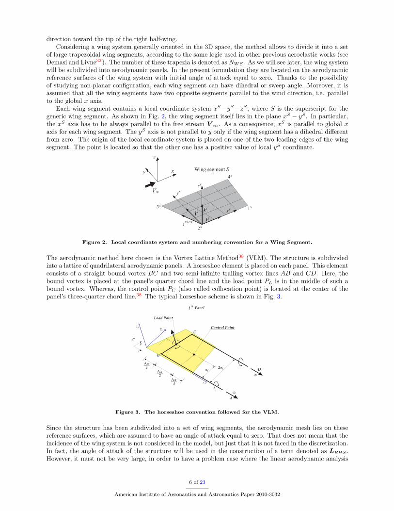
The aerodynamic method here chosen is the Vortex Lattice Method38 (VLM). The structure is subdividedinto a lattice of quadrilateral aerodynamic panels. A horseshoe element is placed on each panel. This elementconsists of a straight bound vortex BC and two semi-infinite trailing vortex lines AB and CD. Here, thebound vortex is placed at the panel’s quarter chord line and the load point PL is in the middle of such abound vortex. Whereas, the control point PC (also called collocation point) is located at the center of thepanel’s three-quarter chord line.38 The typical horseshoe scheme is shown in Fig. 3.

Figure 3. The horseshoe convention followed for the VLM.

Since the structure has been subdivided into a set of wing segments, the aerodynamic mesh lies on thesereference surfaces, which are assumed to have an angle of attack equal to zero. That does not mean that theincidence of the wing system is not considered in the model, but just that it is not faced in the discretization.In fact, the angle of attack of the structure will be used in the construction of a term denoted as LRHS .However, it must not be very large, in order to have a problem case where the linear aerodynamic analysis

6 of 23


remains a valid approximation.For each wing segment it is assigned a straight beam perpendicular to the global x axis and contained in

the plane xS−yS , over which the 1D structural refined elements mesh is created. Each beam element must beentirely contained in a plane orthogonal to the global x axis (wind direction). All the elements constitutingthe whole structural mesh are connected. For instance, Fig. 4 shows the application of the method to atypical C-Wing configuration, which is divided into differently coloured wing segments.

Figure 4. Unidimensional structural mesh and bidimensional aerodynamic mesh of wing segments.

It should be noted that the origin of the coordinate system on the cross-section of a generic finite elementdoes not necessarily coincide with the centroid of the section itself. Moreover, such an origin in general canbe located outside the cross-section area, as shown in Fig. 1.

To summarize, the model studies the deformation of a wing system generally oriented in the 3D spaceby means of refined finite elements in general not lying on the wing surface.

VI. Aeroelastic formulation

At first, the above mentioned structural formulation has to be extended in order to study generally orientedbeam-like structures. In fact, the fundamental nuclei have been obtained in the local coordinate system ofthe element. Considering the generic wing segment S, Eq. 17 written in its local coordinate system becomes:

δLi = δqS Tτi loc K ij τ s S

loc qSsj loc (22)

This expression is in general valid in local coordinate system, whose yS axis is parallel to the element beamaxis. For the general purpose of this work, it is necessary to extend the formulation to the global coordinatesystem. The problem consists in a typical transformation of coordinates by means of orthogonal matrices.Let iS , jS and kS be the unit vectors of the local coordinate system. They are expressed in global coordinatesvia the corresponding unit vectors i, j and k (see Fig. 2):

iS = eS11 i + eS12 j + eS13 k

jS = eS21 i + eS22 j + eS23 k

kS = eS31 i + eS32 j + eS33 k

(23)

where the 9 coefficients are the global coordinates of local unit vectors. By isolating such terms in a matrix3× 3, any vector of local nodal displacements can be expressed in global coordinates as follows:

qSsj loc = eS · qS

sj (24)

The substitution of Eq. 24 in Eq. 22 leads to write the fundamental nucleus of Structural Stiffness Matrixin the global coordinate system:

δLi = δqS Tτi loc K ij τ s S

loc qSsj loc = δqS T

τi

[eS T · K ij τ s S

loc · eS]qSsj (25)

7 of 23


Before the assembly procedure the FE structural matrices must be rotated to impose the compatibility ofthe displacements expressed in global coordinates:

K ij τ s S =[eS T · K ij τ s S

loc · eS]

(26)

The assembly procedure on beam elements of different wing segments will be performed in the classical way,summing up the stiffness terms corresponding to the common nodes.

A. Splining and Pseudo-Structural Points

The coupling of structural and aerodynamic fields is carried out by a splining method. Although thepresent Finite Element Model is unidimensional, the splining is not performed by means of the Beam Splinemethod,33−34 but indeed of the Infinite Plate Spline method35−37 (IPS). The reason is due to the accuracyof refined element in predicting displacements of points not necessarily coincident with the actual FEM nodesand not even located on the element axis.

On the reference plane of each Wing Segment (the generic one is indicated with superscript S) a setof NS

PS aeroelastic points is chosen and the corresponding displacements are computed by the structuralformulation. Then, these deflections will be utilized as input data in order to mathematically describe thedeformed surface of wing segment S via IPS method. The points forming the set are denoted as pseudo-structural points, precisely because they have the meaning of structural points (the spline surface is treatedas a plate by IPS method). The adjective pseudo is adopted to not confuse them with structural nodes ofthe beam elements.

Defining the vector x as the vector which contains the global coordinates of pseudo-structural points ofthe entire wing system, it is possible to extract the global coordinates of the pseudo-structural points locatedon wing segment S and define the vector xS by means of matrix JS . Since the point 2S is the origin ofthe local coordinate system of wing segment S (see Fig. 2), the vector x2S (with dimension 3NS

PS × 1) isintroduced:

x2S =x2S y2S z2S ... x2S y2S z2S

T

(27)

The coordinates xSloc of the pseudo-structural points lying on wing segment S expressed in the local reference

system are determined by defining the block diagonal matrix ES , where the transformation matrix eS isrepeated as many times as NS

PS :

xSloc = ES ·

xS − x2S

= ES ·

JS · x − x2S

(28)

Remembering that q is the vector of the nodal degrees of freedom (in global coordinate system) of all nodeson the beams, it is possible to extract the vector qS of nodal displacements (in global coordinate system)corresponding to wing segment S only, by means of matrix IS .

It is now possible to convert the vector qS in local coordinates using a formula similar to Eq. 24, byintroducing the matrix ES

q . It is a block diagonal matrix containing the transformation matrix eS for eachdegree of freedom of the structural nodes corresponding to wing segment S. Therefore:

qSloc = ES

q · qS = ESq · IS · q (29)

To utilize the Finite Element formulation, it is mandatory to individualize the corresponding finite elementfor each pseudo-structural point. The parameter to be analyzed is the local yS coordinate, which is extractedfrom vector xS

loc. In fact, by using that value it is possible to “assign” that pseudo-structural point to aparticular beam element on wing segment S. Everything is expressed in local coordinates and so the FEMequation 30 can be used to calculate the local displacements according to CUF:

uSloc

(xS , yS , zS

)= Fτ

(xS , zS

)uS

τ loc

(yS

)= Fτ

(xS , zS

)Ni

(yS

)qSloc (30)

The same expression can be repeated for all the pseudo-structural points of wing segment S, noting that eachof them has zero angle of attack and so zS = 0. Resuming Eq. 29, this means that for each wing segment itis possible to define a matrix Y S which relates the vector of nodal degrees of freedom in local coordinates ofwing segment S with the displacements uS

loc (in local coordinates) of all the pseudo-structural points. Then,

8 of 23


calling ISz the constant matrix which allows the extraction of zS component of the local displacements it is

possible to write Eq. 31:

ZSloc = IS

z · uSloc = IS

z · Y S · qSloc = IS

z · Y S · ESq · IS · q (31)

The vector ZSloc in Eq. 31 contains the zS coordinates of the deformed configuration and so the input data

for the spline method. Using the fitted surface spline shape it is possible to calculate the derivatives of sucha shape and the associated local angle of attack. The local z coordinate of the pseudo-structural point i onwing segment S is:

ZSi loc = ZS

i loc

(xSi loc, y

Si loc

)(32)

The assumption that the displacements are not very large is made. In fact, a linear theory is utilized,then it is appropriate to assume small displacements. So, the aerodynamic linear theory holds. Under thisassumption, it is reasonable to consider the local in-plane coordinates of the nodes, the load and controlpoints of a generic wing segment constant. Only the out-of-plane local displacement will be different fromzero. Under this hypothesis, all the splining matrices are constant and they can be calculated once.

According to the IPS method, for each pseudo-structural point i of wing segment S the correspondingZSi loc is written as:

ZSi loc

(xSi loc, y

Si loc

)= aS0 + aS1 xS

i loc + a2 ySi loc +

NSPS∑

j=1

Fj KSij (33)

where:KS

ij =(rSij loc

)2ln(rSij loc

)2(34)(

rSij loc

)2=

(xSi loc − xS

j loc

)2+

(ySi loc − ySj loc

)2(35)

noting that also the counter j refers to pseudo-structural points. For the sake of brevity, the details about theIPS method35−37 are not reported here. Writing Eq. 33 for all the pseudo-structural points and combiningthe infinite conditions, the following matrix notation is obtained:

ZS⋆loc =

0 RS[RS

]TKS

· P S = GS · P S (36)

By inverting Eq. 36, it is possible to find the NSPS + 3 unknowns represented by the spline coefficients P S .

Once obtained the coefficients necessary to describe the spline, then the aerodynamic points of the panelsare taken into account. To impose the boundary conditions the derivatives with respect to xS are requiredat control points. Therefore, it is necessary to differentiate the spline equation 33 with respect to xS andcalculate the result in the local coordinates of control points. Let

(XS

k loc , YSk loc

)be the local coordinates (in

the reference plane) of the kth control point. Its slope is given by:

dZSk loc

dxS

(XS

k loc , YSk loc

)= a1 +

NSPS∑

j=1

Fj DSkj = a1 +

NSPS∑

j=1

Fj

[2(XS

k loc − xSj loc

) [1 + ln

(RS

kj loc

)2 ]](37)where: (

RSkj loc

)2=

(XS

k loc − xSj loc

)2+

(YSk loc − ySj loc

)2(38)

Following the exposed procedure for all the NSAP (= Number of Aerodynamic Panels of wing segment S)

locations on the surface, the slopes can be written as functions of the spline coefficients in a compact form:

dZSloc

dxS= DS · P S (39)

Now, it is advantageous to write an expression able to relate directly the output and the input data, repre-sented by the zS coordinates of pseudo-structural points in the deformed configuration:

dZSloc

dxS= DS · P S = DS ·

[GS

]−1

· ZS⋆loc = DS · SS · ZS

loc (40)

9 of 23


where SS is the matrix[GS

]−1

with the first three columns eliminated, without changing the result.

Combining Eqs. 31 and 40, the following expression relates the slope of control points of all the panels inwing segment S to the vector of nodal degrees of freedom of the whole structure:

dZSloc

dxS= DS · SS · IS

z · Y S · ESq · IS · q = DS aS

3 · q (41)

Equation 41 can be written for all wing segments and so an assembly procedure is required to have all thelocal slopes of all the panels of the entire wing system as a function of degrees of freedom of all the structuralfinite elements.

While calculating the generalized aerodynamic matrices, it is required to transform lift forces at aero-dynamic load points into nodal forces on the structural grid nodes. This transformation will involve thedisplacements of load points. The matrix relating the input displacements at pseudo-structural points to

the output deflections at load points is addressed as DS ⋆

and built following the spline equation 33. Theprocedure needs the local coordinates

(XS

loc , YSloc

)of load points. Finally, the displacement vector at load

points can be written as function of the nodal degrees of freedom by using a procedure formally identical tothe one used to obtain Eq. 41:

ZS

loc = DS ⋆

· P S = DS ⋆

· SS · ISz · Y S · ES

q · IS · q = DS ⋆

aS3 · q (42)

The assembly process is carried out by calculating all the products (for all wing segments) DS aS3 and

DS ⋆

aS3 and observing that each aerodynamic panel can be included only in one trapezoidal wing segment.

In fact, different wing segments don’t share common aerodynamic panels. After the assembly, Eqs. 41 and 42written at wing system level become:

dZ loc

dx= A3 · q (43)

Z loc = A⋆

3 · q (44)

By means of the exposed matricial notation, Eqs. 43 and 44 allow to directly relate displacements and slopesat aerodynamic points of the structure to its nodal degrees of freedom.

B. Steady Aerodynamic Forces

Now the derivation of aerodynamic loads is faced. According to the Vortex Lattice Method,38 the pressuresacting on the deflecting surface are transferred as lift forces located on load points of the aerodynamic panelsof the whole structure. Considering the generic jth panel of wing segment S and dimensionless pressureacting on it, the modulus of the lift force applied at the corresponding load point is given by:∣∣LS

j

∣∣ =1

2ρ∞ V 2

∞ ∆xj 2ej ∆pSj (45)

where the quantity ∆xj is the average chord of the panel and ej refers to its half-length along yS local axis(wing spanwise direction). Since the reference aerodynamic configuration has no angle of attack, it shouldbe noted that lift forces are normal to the panels and perpendicular to the wind direction. Let ∆p be thevector containing the dimensionless pressure loads acting on all the aerodynamic panels of the structure,normalized with respect to the dynamic pressure. The lift forces moduli are written in a matrix form:

L =1

2ρ∞ V 2

∞ ID · ∆p (46)

where ID contains the panels’ geometrical data. The VLM allows to describe the dimensionless normalwash,normalized with respect to V∞, as function of the pressures acting on each aerodynamic panel:

w = AD · ∆p (47)

where AD is the Aerodynamic Influence Coefficient Matrix. It is calculated by using the geometrical dataof the aerodynamic mesh. In the steady case, considering that the structure changes configuration when itdeforms, the boundary condition used for the Vortex Lattice formulation is:

w =dZ loc

dx(48)

10 of 23


Considering small angles of deflection because of the model’s linearity, Eq. 48 means that the dimensionlessnormalwash has to equal the slope at the aerodynamic control point. The boundary condition is not only aconstraint expressing the coupling between aerodynamics and deflection of the structure, but in this case itis the interface able to correlate the lifting surface to the nodal degrees of freedom. As a result, by combiningEqs. 43 and 46 - 48, the vector containing the aerodynamic forces is written as function of nodal degrees offreedom:

L =1

2ρ∞ V 2

∞ ID ·[AD

]−1

· w =1

2ρ∞ V 2

∞ ID ·[AD

]−1

· A3 · q =1

2ρ∞ V 2

∞ c · q (49)

where the matrix c has been conveniently introduced.

C. The Aeroelastic Stiffness Matrix

The aerodynamic forces of Eq. 49 are applied at load points of the aerodynamic panels. They are transferredto the structural nodes using the following algorithm. The result will be a vector of equivalent nodal loads,by means of which the construction of the Aeroelastic Stiffness Matrix will be carried out. From Eq. 49 itis possible to extract the forces applied only on panels of the generic wing segment S:

LS =1

2ρ∞ V 2

∞ cS · q (50)

where cS is directly obtained from c. The lift forces are parallel and perpendicular to the surface representingthe wing segment S, then local xS , yS components of the aerodynamic loads are zero. Hence, LS contains notonly the moduli of the loads on aerodynamic panels of wing segment S, but also their local zS components.

The transfer from loads at the aerodynamic points to the energetically equivalent loads at structuralnodes is performed via the Principle of Virtual Displacements. Resuming Eq. 42, the balance between thevirtual work carried out by lift forces on the virtual variation of displacements of load points and the virtualwork carried out by equivalent nodal forces on the virtual variation of nodal degrees of freedom is writtenas:

δW =δZ

S

loc

T

· LS =D

S ⋆aS3 · δq

T

· LS = δq T ·[aS3

]T·[D

S ⋆]T

· LS = δq T · LSstr (51)

where the virtual variation of nodal degrees of freedom q is considered. The vector LSstr contains the nodal

forces on all structural nodes. The superscript S indicates that only the aerodynamic loads applied at thepanels of wing segment S have been taken into account. Combining Eqs. 51 and 50 it is possible to deduce:

LSstr =

[aS3

]T·[D

S ⋆]T

· LS =1

2ρ∞ V 2

∞

[aS3

]T·[D

S ⋆]T

· cS · q (52)

If all the contributions of all wing segments are added following Eq. 52, the loads on the structural nodes

can be obtained. This operation means that an assembly of the matrices1

2ρ∞ V 2

∞

[aS3

]T·[D

S ⋆]T

· cS is

required. The final assembled matrix is named −K aero, where the negative sign is adopted for the sake ofconvenience. The expression of aerodynamic loads on all the structural nodes after all wing segments havebeen taken into account is:

Lstr = −K aero · q (53)

Such a term can go to the left hand side of the aeroelastic equation system and summed up to the productdue to the Structural Stiffness:

K str · q = Lstr = −K aero · q (54)

or [K str + K aero

]· q = 0 (55)

orKaeroelastic · q = 0 (56)

The isolation of the stiffness matrices in Eq. 55 leads to a unique term, called Aeroelastic Stiffness Matrix.Practically, it substitutes the Structural Stiffness Matrix in the FEM system, so that the stiffness of the

11 of 23


structure is sensible to and inclusive of the aerodynamic loads applied. In this way the deflection due tosuch loads is already taken into account directly in the stiffness of the system.

From Eq. 56 it appears that there is no motion. It occurs because the angle of attack so far consideredis zero. So, there is no motion unless we have external non-aerodynamic loads, i.e. some mechanical loads.To solve this problem, a given known shape of the structure is assigned, for instance, by points havinglocal coordinates xS and yS of pseudo-structural points. Whereas, the zS local out-of-plane coordinatesare not equal to zero and describe a shape with different from zero angle of attack. The new points willbe denoted as perturbed pseudo-structural points. The corresponding aerodynamic loads are computed asconcentrated forces localized on the load points and are transformed as energetically equivalent loads at thestructural nodes. Following the same procedure used to find the Aeroelastic Stiffness Matrix, the loads LRHS

on the structural nodes can be obtained (the subscript RHS means Right Hand Side). At the end, the finalaeroelastic equation to be solved is: [

K str + K aero

]· q = LRHS (57)

orKaeroelastic · q = LRHS (58)

Equation 58 allows to compute the vector of unknown nodal degrees of freedom q. Now that the right handside is different from zero, we have a solution.

VII. Results

The structural and aeroelastic results are presented here. The analyses have been executed on a seriesof different geometrical configurations. The beam’s cross-sections analyzed in this work are rectangularor square and clamped boundary condition is accounted for. An isotropic material is used. The Young’smodulus E is equal to 69 [GPa] and the Poisson’s ratio ν is equal to 0.33. For the exposed results a selectiveintegration of the shape functions along the beam axis is adopted.

The structural assessment of the refined finite element is carried out in order to validate its propriety incomparison with some classical analytical results and NASTRAN simulations. Beams subjected to bendingand torsional loadings are analyzed. As far as the aeroelastic assessment is concerned, some aeroelasticanalyses have been performed on planar and non-planar wing configurations. The corresponding resultshave been validated with NASTRAN.

A. Structural Assessment

For the first structural assessment, the beam’s rectangular cross-section has dimension 3×60 [mm], whereasthe length L is equal to 600 [mm]. For example, the beam could simulate the wind tunnel model for a glinderwing. The loading condition is a pure bending about the local xS axis. The concentrated bending load Puz

(equal to 1N) acts on the centroid of the tip cross-section. The mechanics of the beam is described in termsof dimensionless maximum vertical displacement, uzmax, which is computed at the center point of the tipcross-section. Such a dimensionless displacement is normalized with respect to the following value given bythe Euler-Bernoulli beam theory, which is taken as reference solution:

u ⋆zmax =

Puz L3

3 E I= 7.7295mm u ⋆

zmax = 1.0000 (59)

where I is the moment of inertia of the beam cross-section. A structural convergence study is carried outto evaluate the effect of the number of Finite Elements NEL constituting the structural mesh on results.Then, a further structural convergence study on the effect of the expansion order N defining the UnifiedFormulation is performed. Such convergence analyses are conducted for the three elements B4, B3, B2, with4, 3, 2 nodes respectively. Their results are shown in Tables 2 - 4.

According to the typical behavior of FEM solutions, the maximum tip displacement increases and becomesmore accurate as NEL increases. An excellent agreement is obtained between the refined model’s andNASTRAN results, which are slightly different from the approximated Euler-Bernoulli solution of Eq. 59.When the expansion order is N = 4, Fig. 5 describes the behavior of the solution when the number ofelements (B2, B3 and B4) increases and proves graphically such an agreement. The results and the accuracy

12 of 23


of the structural model change as N changes. Anyway, after N = 3 the final result appears not to beevidently variable and then the convergence on N is reached. Finally, the deflection along the beam axis isinvestigated in Fig. 6.

As second load case, the cantilever beam is subjected to a torsional loading located on the tip cross-section. The previous beam has been replaced with a square cross-section beam, but keeping the samelenght. It results to be slender with a high span-to-height ratio. The load is reproduced by two oppositeconcentrated forces acting on two points of the tip cross-section symmetrical with respect to the vertical zaxis.

The investigation about the effect of expansion orderN on the deflection of tip cross-section is summarizedin Fig. 7. The first-order theory predicts the planarity of the cross-section in the deformed configuration.Second and third-order models yield similar results, with the deformation no more planar. Finally, thefourth-order clearly shows the warping effect on the tip cross-section. Hence, the deformed section has nota planar behavior, differently from the first-order theory and classical models. It has been demonstratedthat the refined model for higher-order expansion is able to study beam-like structures more accuratelythan the classical models, highlighting the out-of-plane displacements of beam cross-sections. Then, theUnified Formulation provides an approximation of the tridimensional structural behavior in spite of theunidimensional discretization.

B. Aeroleastic Assessment

The aeroelastic assessment has the goal to validate the aeroelastic model by comparison with NASTRANsolutions (SOL 144). It is performed a convergence study similar to the analyses carried out for the struc-tural assessment. Now, such a study evaluates the correctness of the interaction between structures andaerodynamics. For this purpose, the convergence on the number of aerodynamic VLM panels NAP used todiscretize the reference surfaces of wing segments is also investigated.

Here, the cases considered consist in three different wing configurations. The static aeroelastic responsesof an unswept wing, a straight wing with dihedral and a swept tapered wing are investigated. In fact, thepresent beam formulation would be able to analyse a number of non-planar combinations of swept, tapered,dihedral wing segments. By exploiting the powerful of the method, the problem is solved by using righthalf-wing of each system only. Therefore, the aerodynamic computation takes into account the symmetrycondition. The cross-section is always rectangular with thickness equal to 3 [mm]. For first two cases thechord is constant and equal to 60 [mm], whereas the root and tip chords for the tapered wing are 100 [mm]and 40 [mm] respectively (see Fig. 8). The wingspan b does not change for the three cases and is equal to1200 [mm]. The dihedral angle Γ used in case 2 is equal to 20 [deg].

For the previous assessment the input loads were only mechanical and not aerodynamic. Now, the si-tuation is opposite, since the only input load consists in the fact that the wing system is exposed to thefree stream. Its velocity is equal to 40 [m/s] and the considered air density is equal to 1.225 [kg/m3]. Theangle of attack for all the treated cases is equal to 1 [deg]. Again the mechanics of the beam is describedin terms of the maximum vertical displacement, uzmax, which now is computed on the leading edge of thetip section. The analyses have been carried out by using the more accurate B4 element and its convergencefor each aeroelastic case is reported on Tables 5, 7 and 9. Also for these aeroelastic problems, the maximumtip displacement increases for higher-order theories and becomes more accurated as NEL increases. It is tonote how the swept tapered requires a slightly greater number of elements to reach convergence, due to itsparticular geometry.

For the investigated cases, Tables 6, 8 and 10 summarize the values of static aeroelastic deflections asthe number of aerodynamic VLM panels increases. Moreover, it is reported the trend as the expansionorder N of the theory changes. The results are validated with commercial code NASTRAN (sol 144), whichhas performed aeroelastic analysis by coupling Doublet Lattice Method and structural shell elements. Asexpected, the solution approaches to more realistic values as the number of aerodynamic elements increases.Such a convergent trend occurs for all the shown theories, but well agreement between the aeroelastic model’sand NASTRAN results is obtained only when higher-order theories are involved. In particular, the typicaltorsional effect about y axis due to aerodynamic loadings is more accurately highlighted for large values ofN . For swept tapered wings such an effect is presented in Fig. 11, whereas the tridimensional deflections ofcases 1 and 3 are shown in Fig. 9 and 10.

13 of 23


Convergence study for Element B4

Load case: Bending u ⋆zmax = 1.0000 NASTRAN: 0.9880

NEL EBBM TBM N = 1 N = 2 N = 3 N = 4

2 0.9999 1.0000 1.0000 0.9344 0.9601 0.9604

5 1.0000 1.0000 1.0000 0.9486 0.9766 0.9776

10 1.0000 1.0000 1.0000 0.9532 0.9813 0.9826

20 1.0000 1.0000 1.0000 0.9555 0.9836 0.9850

40 1.0000 1.0000 1.0000 0.9567 0.9848 0.9862

Table 2. Structural case: Effect of the number of B4 elements on uz max.



NEL EBBM TBM N = 1 N = 2 N = 3 N = 4

2 0.9999 1.0000 1.0000 0.9110 0.9307 0.9307

5 1.0000 1.0000 1.0000 0.9403 0.9669 0.9674

10 1.0000 1.0000 1.0000 0.9492 0.9772 0.9782

20 1.0000 1.0000 1.0000 0.9535 0.9816 0.9829

40 1.0000 1.0000 1.0000 0.9557 0.9838 0.9852




NEL EBBM TBM N = 1 N = 2 N = 3 N = 4

2 0.9375 0.9375 0.9375 0.7907 0.7978 0.7978

5 0.9900 0.9900 0.9900 0.9035 0.9238 0.9240

10 0.9975 0.9975 0.9975 0.9332 0.9583 0.9589

20 0.9994 0.9994 0.9994 0.9462 0.9735 0.9745

40 0.9996 0.9999 0.9999 0.9522 0.9801 0.9813


14 of 23


5 10 15 20 25 30 35 400.75

0.8

0.85

0.9

0.95

1

1.05

Number of elements NEL

Dim

ensi

onle

ss tr

ansv

erse

dis

plac

emen

t uz

Convergence for Refined Beam Elements B2, B3, B4 N = 4

Refined Element B2Refined Element B3Refined Element B4NASTRAN SolutionEuler−Bernoulli Beam Solution

Figure 5. Convergence study for Refined Elements.

Figure 6. Deflection of the beam utilized for the convergence study.

15 of 23


Figure 7. Deformed tip cross-section of the beam subjected to torsional load as N increases.

VV

VV

Figure 8. Wing configurations considered for the aeroelastic analysis.

16 of 23


Aeroelastic case 1: straight wing

Stream Velocity : 40 m/s α = 1 deg NASTRAN: 9.1500

NEL EBBM TBM N = 1 N = 2 N = 3 N = 4

2 8.8074 8.8076 8.8123 8.5268 8.7961 8.8019

5 8.8073 8.8075 8.8122 8.7092 9.0097 9.0243

10 8.8073 8.8075 8.8122 8.7685 9.0710 9.0895

20 8.8072 8.8075 8.8122 8.7980 9.1012 9.1209

40 8.8071 8.8075 8.8122 8.8126 9.1164 9.1369

Table 5. Convergence study: Effect of the number of B4 elements on uz max [mm]. Aerodynamic mesh: 6 × 60VLM panels. Symmetry enabled.

Aeroelastic case 1: straight wing

Stream Velocity : 40 m/s α = 1 deg

NPANELS EBBM TBM N = 1 N = 2 N = 3 N = 4 NASTRAN

2× 20 8.9903 8.9904 8.9953 8.9936 9.3029 9.3231 9.3253

4× 40 8.8545 8.8546 8.8594 8.8473 9.1521 9.1719 9.2004

6× 60 8.8072 8.8075 8.8122 8.7980 9.1012 9.1209 9.1500

10× 100 8.7679 8.7681 8.7727 8.7565 9.0585 9.0781 9.1083

Table 6. Convergence study: Effect of the number of aerodynamic VLM panels on uz max [mm]. Structural mesh:20 elements B4. Symmetry enabled.

Aeroelastic case 2: straight wing with dihedral


NEL EBBM TBM N = 1 N = 2 N = 3 N = 4

2 10.7476 10.7478 10.7543 10.5085 10.8235 10.8303

5 10.7475 10.7476 10.7542 10.7334 11.0902 11.1071

10 10.7471 10.7474 10.7542 10.8063 11.1661 11.1880

20 10.7481 10.7488 10.7542 10.8425 11.2033 11.2268

40 10.7549 10.7535 10.7542 10.8606 11.2220 11.2465


17 of 23


Aeroelastic case 2: straight wing with dihedral



2× 20 10.9702 10.9710 10.9766 11.0845 11.4524 11.4765 11.4779

4× 40 10.8050 10.8057 10.8114 10.9033 11.2658 11.2894 11.3277

6× 60 10.7481 10.7488 10.7542 10.8425 11.2033 11.2268 11.2659

10× 100 10.7000 10.7011 10.7063 10.7914 11.1507 11.1740 11.2148

Table 8. Convergence study: Effect of the number of aerodynamic VLM panels on uz max [mm]. Structural mesh:20 elements B4. Symmetry enabled.

Aeroelastic case 3: swept tapered wing


NEL EBBM TBM N = 1 N = 2 N = 3 N = 4

2 6.4814 6.4816 6.4837 6.1732 6.5183 6.5282

5 6.1779 6.1780 6.1800 6.0000 6.3359 6.3505

10 6.1352 6.1354 6.1373 6.0011 6.3344 6.3490

20 6.1246 6.1248 6.1267 6.0110 6.3464 6.3602

40 6.1220 6.1221 6.1240 6.0181 6.3542 6.3680


Aeroelastic case 3: swept tapered wing



2× 20 6.2274 6.2275 6.2295 6.1197 6.4629 6.4771 6.4791

4× 40 6.1513 6.1514 6.1533 6.0386 6.3755 6.3894 6.4093

6× 60 6.1246 6.1248 6.1267 6.0110 6.3464 6.3602 6.3806

10× 100 6.1020 6.1022 6.1040 5.9875 6.3215 6.3354 6.3566

Table 10. Convergence study: Effect of the number of aerodynamic VLM panels on uz max [mm]. Structuralmesh: 20 elements B4. Symmetry enabled.

18 of 23


Figure 9. Aeroelastic deflection of the straight wing for case 1 (α = 1).

19 of 23


Figure 10. Aeroelastic deflection of the swept tapered wing for case 3 (α = 1).

DEFORMED

WING

UNDEFORMED WING

Figure 11. Torsional effect on tip cross-section of the swept tapered wing.

20 of 23


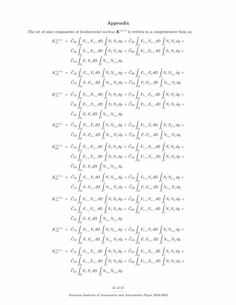
Appendix

The set of nine components of fundamental nucleus K ij τ s is written in a comprehensive form as:

K ij τ sxx = C22

∫Ω

Fτ,x Fs,x dΩ

∫l

Ni Nj dy + C26

∫Ω

Fτ,z Fs,x dΩ

∫l

Ni Nj dy +

C26

∫Ω

Fτ,x Fs,z dΩ

∫l

Ni Nj dy + C66

∫Ω

Fτ,z Fs,z dΩ

∫l

Ni Nj dy +

C44

∫Ω

Fτ Fs dΩ

∫l

Ni,y Nj,y dy

K ij τ sxy = C23

∫Ω

Fτ,x Fs dΩ

∫l

Ni Nj,y dy + C36

∫Ω

Fτ,z Fs dΩ

∫l

Ni Nj,y dy +

C45

∫Ω

Fτ Fs,z dΩ

∫l

Ni,y Nj dy + C44

∫Ω

Fτ Fs,x dΩ

∫l

Ni,y Nj dy

K ij τ sxz = C12

∫Ω

Fτ,x Fs,z dΩ

∫l

Ni Nj dy + C16

∫Ω

Fτ,z Fs,z dΩ

∫l

Ni Nj dy +

C26

∫Ω

Fτ,x Fs,x dΩ

∫l

Ni Nj dy + C66

∫Ω

Fτ,z Fs,x dΩ

∫l

Ni Nj dy +

C45

∫Ω

Fτ Fs dΩ

∫l

Ni,y Nj,y dy

K ij τ syx = C45

∫Ω

Fτ,z Fs dΩ

∫l

Ni Nj,y dy + C44

∫Ω

Fτ,x Fs dΩ

∫l

Ni Nj,y dy +

C23

∫Ω

Fτ Fs,x dΩ

∫l

Ni,y Nj dy + C36

∫Ω

Fτ Fs,z dΩ

∫l

Ni,y Nj dy

K ij τ syy = C55

∫Ω

Fτ,z Fs,z dΩ

∫l

Ni Nj dy + C45

∫Ω

Fτ,x Fs,z dΩ

∫l

Ni Nj dy +

C45

∫Ω

Fτ,z Fs,x dΩ

∫l

Ni Nj dy + C44

∫Ω

Fτ,x Fs,x dΩ

∫l

Ni Nj dy +

C33

∫Ω

Fτ Fs dΩ

∫l

Ni,y Nj,y dy

K ij τ syz = C55

∫Ω

Fτ,z Fs dΩ

∫l

Ni Nj,y dy + C45

∫Ω

Fτ,x Fs dΩ

∫l

Ni Nj,y dy +

C13

∫Ω

Fτ Fs,z dΩ

∫l

Ni,y Nj dy + C36

∫Ω

Fτ Fs,x dΩ

∫l

Ni,y Nj dy

K ij τ szx = C12

∫Ω

Fτ,z Fs,x dΩ

∫l

Ni Nj dy + C26

∫Ω

Fτ,x Fs,x dΩ

∫l

Ni Nj dy +

C16

∫Ω

Fτ,z Fs,z dΩ

∫l

Ni Nj dy + C66

∫Ω

Fτ,x Fs,z dΩ

∫l

Ni Nj dy +

C45

∫Ω

Fτ Fs dΩ

∫l

Ni,y Nj,y dy

K ij τ szy = C13

∫Ω

Fτ,z Fs dΩ

∫l

Ni Nj,y dy + C36

∫Ω

Fτ,x Fs dΩ

∫l

Ni Nj,y dy +

C55

∫Ω

Fτ Fs,z dΩ

∫l

Ni,y Nj dy + C45

∫Ω

Fτ Fs,x dΩ

∫l

Ni,y Nj dy

K ij τ szz = C11

∫Ω

Fτ,z Fs,z dΩ

∫l

Ni Nj dy + C16

∫Ω

Fτ,x Fs,z dΩ

∫l

Ni Nj dy +

C16

∫Ω

Fτ,z Fs,x dΩ

∫l

Ni Nj dy + C66

∫Ω

Fτ,x Fs,x dΩ

∫l

Ni Nj dy +

C55

∫Ω

Fτ Fs dΩ

∫l

Ni,y Nj,y dy

21 of 23


References

1Livne E., Weisshaar T.A., “Aeroelasticity of Nonconventional Airplane Configurations-Past and Future”, Journal ofAircraft, Vol. 40, No. 6, 2003, pp. 1047-1065.

2Frediani A., Rizzo E., Bottoni C., Scanu J., Iezzi G., “A 250 Passenger Prandtlplane Transport Aircraft PreliminaryDesign”, Aerotecnica Missili e Spazio (AIDAA), Vol. 84, No. 4, September 2005.

3Livne E.,“Future of Airplane Aeroelasticity”, Journal of Aircraft, Vol. 40, No. 6, 2003, pp. 1066-1092.4Demasi L., Livne E., “Exploratory Studies of Joined Wing Aeroelasticity”, 46th AIAA/ASME/ASCE/AHS/ASC Struc-

tures, Structural Dynamics, and Materials Conference, Austin, TX, AIAA Paper 2005-2172, April 2005.5Patil M. J., Hodges D. H. and Cesnik C. E. S., “Nonlinear Aeroelasticity and Flight Dynamics of High-Altitude Long-

Endurance Aircraft”, Journal of Aircraft, Vol. 38, No. 1, 2001, pp. 88-94.6Patil M. J., Hodges D. H. and Cesnik C. E. S., “Limit Cycle Oscillations in High-Aspect-Ratio Wings”, Journal of Fluids

and Structures, Vol. 15, No. 1, 2001, pp. 107-132.7Sulaeman E., Kapania R. and Haftka R. T., “Parametric Studies of Flutter Speed in a Strut-braced Wing”, 43rd

AIAA/ASME/ASCE/AHS/ASC Structures, Structural Dynamics, and Materials Conference, Denver, CO, AIAA Paper 2002-1487, April 2002.

8Sulaeman E., “Effect of Compressive Force on Aeroelastic Stability of a Strut-Braced Wing”, Ph.D Dissertation, VirginiaPolytechnic Inst. and State Univ., Blacksburg, VA, November 2001.

9Bhatia M., Kapania K., Van Hoek M. and Haftka R., “Structural Design of a Truss Braced Wing: Potential and Chal-lenges”, 50rd AIAA/ASME/ASCE/AHS/ASC Structures, Structural Dynamics, and Materials Conference, Palm Springs, CA,AIAA Paper 2009-2147, May 2009.

10Demasi L., Livne E., “Aeroelastic Coupling of Geometrically Nonlinear Structures and Linear Unsteady Aerodynamics:Two formulations”, Journal of Fluids and Structures, Vol. 25, 2009, pp. 918-935.

11Hodges D. H., “A Mixed Variational Formulation Based on Exact Intrinsic Equations for Dynamics of Moving Beams”,International Journal of Solids and Structures, Vol. 26, No. 11, 1990, pp. 1253-1273.

12Kapania K., Raciti S., “Recent Advances in Analysis of Laminated Beams and Plates, Part I: Shear Effects and Buckling”,AIAA Journal, Vol. 27, No. 7, 1989, pp. 923-935.

13Kapania K., Raciti S., “Recent Advances in Analysis of Laminated Beams and Plates, Part II: Vibrations and WavePropagation”, AIAA Journal, Vol. 27, No. 7, 1989, pp. 935-946.

14Kim G., White S. R., “Thick-Walled Composite Beam Theory Including 3D Elastic Effects and Torsional Warping”,International Journal of Solids and Structures, Vol. 34, No. 31-32, 1997, pp. 4237-4259.

15Reddy J. N., “On Locking-Free Shear Deformable Beam Finite Elements”, Computer Methods in Applied Mechanicsand Engineering, Vol. 149, 1997, pp. 113-132.

16Lee J., “Flexural Analysis of Thin-Walled Composite Beams Using Shear-Deformable Beam Theory”, Composite Struc-tures, Vol. 70, No. 2, 2005, pp. 212-222.

17Volovoi V. V., Hodges D. H., Berdichevsky V. L. and Sutyrin V. G., “Asymptotic Theory for Static Behavior of ElasticAnisotropic I-beams”, International Journal of Solid Structures, Vol. 36, 1999, pp. 1017-1043.

18Volovoi V. V., Hodges D. H., “Theory of Anisotropic Thin-Walled Beams”, Journal of Applied Mechanics, Vol. 67, 2000,pp. 453-459.

19Yu W., Volovoi V. V., Hodges D. H., and Hong X., “Validation of the Variational Asymptotic Beam Sectional Analysis(VABS)”, AIAA Journal, Vol. 40, No. 10, 2002, pp. 2105-2113.

20Carrera E., “Theories and Finite Elements for Multilayered Plates and Shells: a Unified Compact Formulation withNumerical Assessment and Benchmarking”, Archives of Computational Methods in Engineering, Vol. 10, No. 3, 2003, pp.215-296.

21Reddy J. N., “Mechanics of Laminated Composite Plates and Shells. Theory and Analysis”, CRC Press, 2nd Edition,Florida, 2004.

22Jones R., “Mechanics of Composite Materials”, Taylor & Francis, 2nd Edition, Philadelphia, PA, 1999.23Timoshenko S. P., “Strength of Materials”, Van Nostrand company, New York, 1940.24Carrera E., Brischetto S. , “Analysis of Thickness Locking in Classical, Refined and Mixed Multilayered Plate Theories”,

Composite Structures, Vol. 82, No. 4, 2008, pp. 549-562.25Carrera E., Brischetto S., “Analysis of Thickness Locking in Classical, Refined and Mixed Theories for Layered Shells”,

Composite Structures, Vol. 85, No. 1, 2008, pp. 83-90.26Giunta G., Carrera E. and Belouettar S., “A Refined Beam Theory with only Displacement Variables and Deformable

Cross-Section”, 50th AIAA/ASME/ASCE/AHS/ASC Structures, Structural Dynamics, and Materials Conference, PalmSprings, CA, AIAA Paper 2009-2370, May 2009.

27Carrera E., Demasi L., “Classical and Advanced Multilayered Plate Elements Based upon PVD and RMVT. Part 1:Derivation of Finite Element Matrices”, International Journal for Numerical Methods in Engineering, Vol. 55, 2002, pp.191-231.

28Carrera E., Demasi L., “Classical and Advanced Multilayered Plate Elements Based upon PVD and RMVT. Part 2:Numerical Implementations”, International Journal for Numerical Methods in Engineering, Vol. 55, 2002, pp. 253-291.

29Carrera E., Giunta G., Nali M. and Petrolo M., “Refined Beam Elements with Arbitrary Cross-Section Geometries”,Computers and Structures, Vol. 88, No. 5-6, 2009, pp. 283-293.

30Carrera E., Petrolo M. and Nali M., “Unified Formulation Applied to Free Vibrations Finite Element Analysis of Beamswith Arbitrary Section”, Shock and Vibration, in press, 2010.

31Bathe K.J., “Finite Element Procedure”, Prencite Hall, New Jersey, July 1995.32Demasi L., Livne E., “Dynamic Aeroelasticity of Structural Nonlinear Configurations Using Linear Modally Reduced

Aerodynamic Generalized Forces”, AIAA Journal, Vol. 47, No. 1, 2009, pp. 71-90.

22 of 23


33Harder R., MacNeal R. and Rodden W., “A Design for the Incorporation of Aeroelastic Capability into NASTRAN”,report NASA N71-33303, May 1977.

34Rodden W., Harder R. and Bellinger D., “Aeroelastic Addiction to NASTRAN”, NASA contractor report 3094, March1979.

35Harder R., Desmarais R. N., “Interpolation Using Surface Splines”, Journal of Aircraft, Vol. 9, No. 2, 1972, pp. 189-192.36ZONA Technology, Inc., “Spline Methods for Spline Matrix Generation”, ZAERO Theoretical Manual, Ver. 7.1, 2004.37MacNeal-Schwendler corp., “Interconnection of the Structure with Aerodynamics”, MSC.NASTRAN Theoretical Manual,

Ver. 68, Los Angeles, CA, 1994.38Katz J., Plotkin A., “Low-Speed Aerodynamics”, McGraw-Hill, New York, 1991.

23 of 23


Documents

An Improved Beam Formulation for Aeroelastic Applications · An Improved Beam Formulation for Aeroelastic Applications ... structural and aerodynamic ﬁelds is performed via the