Embed Size (px)
Citation preview
ORIGINAL ARTICLE
An improved correlation model for sedimentdelivery ratio assessment
Nazzareno Diodato Æ Sergio Grauso
Received: 14 October 2008 / Accepted: 10 December 2008 / Published online: 27 January 2009
� Springer-Verlag 2009
Abstract In the present work, a new simplified model
approach for sediment delivery ratio (SDR) assessment is
proposed. Modelling and assessing SDR is still an open
question. Difficulties rise from the lack of sufficient data
availability, on one side, and, on the other, from the
inherent uncertainties including spatial variability and
temporal discontinuity of the land cover, climatic, hydro-
logical and geomorphological variables involved. The
proposed SDRSIM model tries to skip over the limitations
observed in other models generally adopted. A comparison
with two different selected models amongst the most
widespread simplified models, i.e. the area-model and the
slope-model, is showed in application to a wide range of
catchments extensions across different landscapes of Italy.
The SDRSIM estimates were also evaluated against
observed SDR over a validation dataset of 11 basins sparse
over different regions of the world. The results showed the
effectiveness of the proposed model approach based on
easily available catchment parameters.
Keywords Sediment delivery � Prediction models �Catchments � Italy
Introduction
Soil erosion rate and river sediment yield are key-factors
whose estimate is essential in land and river systems
management aimed to achieve the environmental sustain-
ability of human activities. Often, given the lack of direct
data, estimates are made by means of prediction models
allowing to evaluate soil loss or sediment yield separately.
There are a number of prediction models, conceptual,
empirical or physically based which can help in this task
that have been successfully tested and are currently used in
different parts of the world. Therefore, one can conclude
that modelling such processes is now an almost achieved
result. On the contrary, linking the two processes of sedi-
ment production and delivery is still an open question.
In fact, it is not unusual that one, being provided with
catchment soil loss data, has the need to convert these data
in sediment yield delivered at a given river section or vice
versa. Nevertheless, to date, there is not a general agree-
ment about an universal model which can suitably explain
the relationship between sediment yield and related upland
soil erosion allowing to convert one quantity into the other
as needed.
The river sediment yield can be defined as the total
quantity of sediments eroded from the upland catchment
area (referred to as gross erosion) which is routed to the
basin outlet by the watercourse in a definite time period.
The sediment yield per unit catchment area is the specific
sediment yield (SSY). Considering that only a partial
amount of gross erosion is routed to the basin outlet
(otherwise referred to as the net erosion), knowing the ratio
between the net erosion and the gross erosion amounts,
which is worldwide known as the sediment delivery ratio
or SDR, is crucial for scientific and management purposes.
As already pointed out by Lu et al. (2004), methods for
N. Diodato
TEDASS – Technologies Interdepartmental Center
for Environmental Diagnostic and Sustainable Development,
University of Sannio, 82100 Benevento, Italy
e-mail: [email protected]
S. Grauso (&)
Dipartimento Ambiente, Cambiamenti Globali e Sviluppo
Sostenibile, ENEA C.R. Casaccia, via Anguillarese 301,
00123 Rome, Italy
e-mail: [email protected]
123
Environ Earth Sci (2009) 59:223–231
DOI 10.1007/s12665-009-0020-x
estimating the SDR can be roughly grouped into three
categories characterized by different degrees of com-
plexity. So, one can distinguish methods, such as sediment
rating curve-flow duration and reservoir sediment deposi-
tion (Collins and Walling 2004; Fan et al. 2004), which
imply that sufficient sediment yield and streamflow data
are available. Sediment yield data are available for many
areas of the world, but the global coverage currently is
inadequate to produce a reliable and detailed world map of
sediment yield (Mutchler et al. 1994). Therefore, such
approaches are not suitable for the general use, because of
data unavailability, especially at the subcatchment level.
A different approach is showed by methods based on
empirical relationships relating the SDR to the morpho-
logical characteristics of a catchment, such as the
catchment area, average local relief or lithology. These
models are largely followed, given their simplified form
requesting easily available data. The general limitation of
these methods is given by the local influence of climatic
and geomorphological characteristics which make a given
relationship unsuitable in geographical areas different from
the area where the relationship was calibrated.
Other methods attempt to provide a physical description
of fundamental hydrological and hydraulic processes, i.e.
by coupling runoff and erosion/deposition processes con-
ditioning the sediment transport capacity. Nevertheless,
their data requirements often make these complex models
not suited to basin scale applications.
In order to overcome some of the difficulties mentioned
above, several attempts to predict the export of sediment
from catchments, by coupling catchment gross erosion to a
SDR value in a spatially distributed modelling approach,
have been investigated. A summary of the relevant litera-
ture is given by Lenhart et al. (2005). Complex and
theoretically based relationships for evaluating the sedi-
ment delivery ratio of each morphological unit into which
the basin can be divided have been proposed in different
way. For example, Ferro and Minacapilli (1995) developed
a model for which SDR is linked to the travel time from the
morphological unit by an exponential relationship. A SDR
model which is used in the Soil and Water Assessment
Tool (SWAT) was proposed by Arnold et al. (1996), taking
into account the peak runoff rate and the peak rainfall
excess rate. Asselman et al. (2003), provided for a SDR
model estimating the amount of mobilized sediment that
actually reaches the stream network, and Borselli et al.
(2004) used a complex connectivity index. New advances
in this field are being gathered thanks to GIS technology
allowing to easily apply different models in a spatially
distributed form (Ouyang and Bartholic 1997).
However, the SDR still remains hard for assessing, as its
estimate implies numerous uncertainties including tempo-
ral discontinuity and spatial variability characterizing the
land cover, climatic, hydrological and geomorphological
variables involved (Wolman 1977; Walling 1983).
As it will be cited in the following sections, many
on-site investigations have been carried out at different
scales, from small farm-plots to small-medium basins up to
large rivers, concerning the linkage between soil erosion
sub-processes on hillslopes and suspended sediment
transport, in the effort to set up a general theoretical model
allowing to indirectly obtain the SDR value and to derive
one of the cited quantities from the other.
In the present work, a new simplified model approach
(SDRSIM) is proposed trying to skip over the limitations
observed in other models generally adopted. In particular, a
comparison with two different selected models amongst the
most widespread simplified models in the international
literature, such as those here referred to as the area-model
(SDRA) and the slope model (SDRSlope), is showed in
application to a wide range of catchments from 1 to
3,000 km2 across different landscapes of Italy. The
SDRSIM estimates were also evaluated against SDR over a
validation dataset of 11 basins sparse over different regions
of the world.
Approach and methodology
Study area and data sources
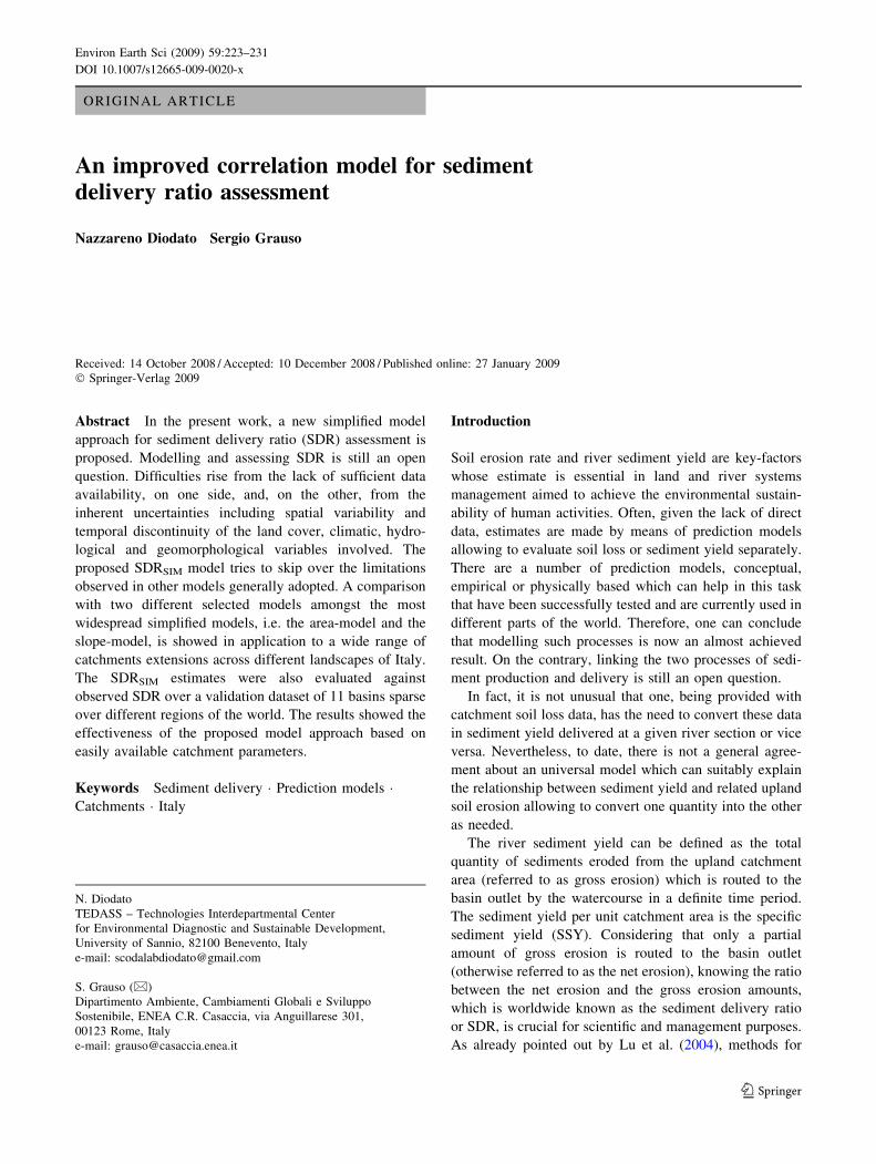
The study was based on data from 25 Italian river basins
located from north to south of Italian peninsula and major
islands (Fig. 1). Italy is centrally placed in the Mediterra-
nean basin and characterized by land use diversity and a
heterogeneous mix of geographical features (peninsular
shape, Alps chain in the north, Apennines chain all along
the peninsula) determined by a large latitudinal gradient
along a relatively narrow land surface, with transition
zones from semi-arid to humid mountain climate (Lionello
et al. 2006).
Such landscape heterogeneity generates greatly varying
ecological and land-degradation patterns at all spatial and
temporal scales with water erosion recognized as the major
land-degradation cause.
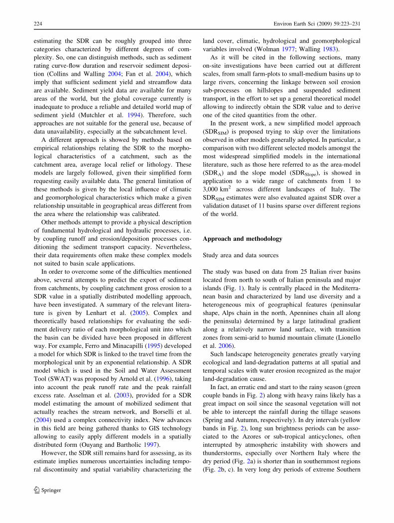
In fact, an erratic end and start to the rainy season (green
couple bands in Fig. 2) along with heavy rains likely has a
great impact on soil since the seasonal vegetation will not
be able to intercept the rainfall during the tillage seasons
(Spring and Autumn, respectively). In dry intervals (yellow
bands in Fig. 2), long sun brightness periods can be asso-
ciated to the Azores or sub-tropical anticyclones, often
interrupted by atmospheric instability with showers and
thunderstorms, especially over Northern Italy where the
dry period (Fig. 2a) is shorter than in southernmost regions
(Fig. 2b, c). In very long dry periods of extreme Southern
224 Environ Earth Sci (2009) 59:223–231
123
Italy and major islands (Fig. 2d), precipitations are inher-
ently variable in amount and intensity and, as a
consequence, the same variability affects rainfall and run-
off erosivity in a very chaotic way.
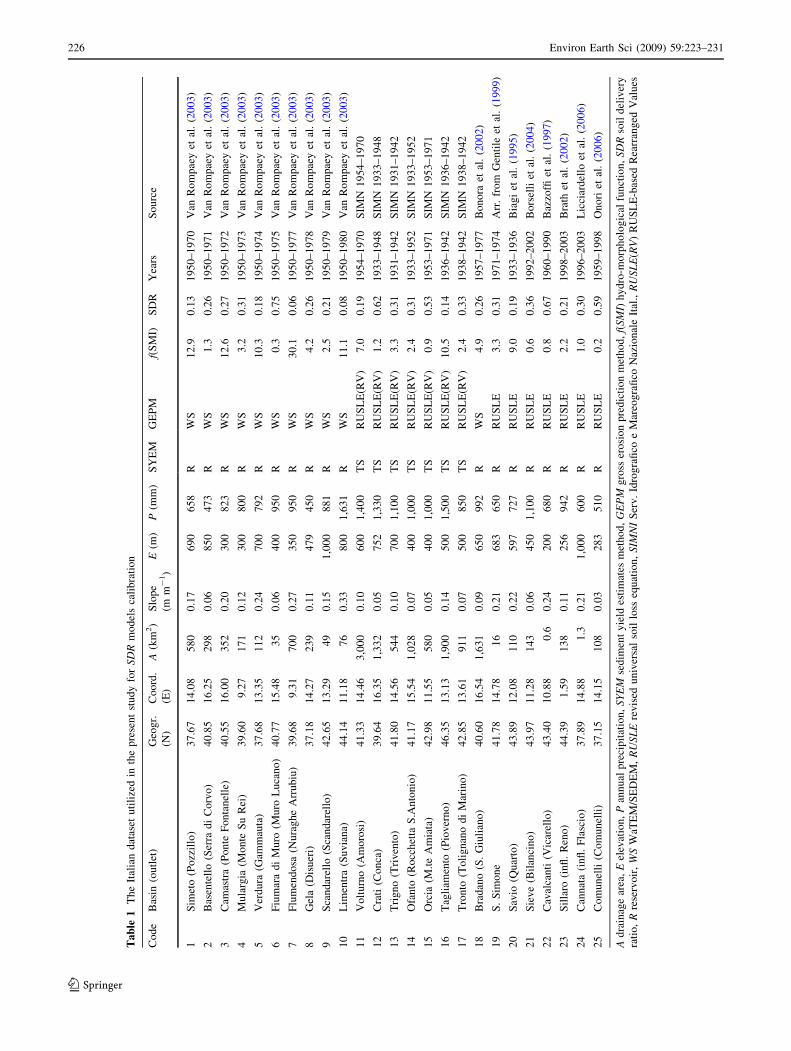
The 25 Italian river basins calibration dataset here uti-
lized (Table 1) is a combination of different data sources
available from the literature or from official sites. Of
course, the sediment yield was measured by means of
different techniques, ranging from reservoir sedimentation
measurements to turbidity measurements, whilst the hill-
slope gross erosion was indirectly assessed by means of
RUSLE model and its different versions. Ten basins were
extracted from the dataset by Van Rompaey et al. (2003)
and de Vente and Poesen (2005), who analysed a series of
watershed-reservoir systems where observed sedimentation
volumes were available. Other eight watershed-reservoir
Fig. 1 Location of the Italian
sediment yield sampling sites
(circles) with related land-
use pattern (in colours)
(see Table 1 for sites coding).
Land-cover source:
http://hydis.eng.uci.edu/gwadi
Humid period
Growing period
Dray period
ETo
0.5 x ETo
5
4
3
2
0
1
5
4
3
2
0
1
6
4
2
0
5
4
3
2
0
1
ETo
0.5 x ETo
(a) (b)
(c) (d)
Precipitation
Precipitation
Humid period
Growing period
Dray period
Fig. 2 Seasonal bioclimatic regime for different location of Italy: a Loiano (Northern Apennines), b Trivento (Central Apennines), c Grassano
(Southern peninsular Italy) and d Caltanissetta (Sicily island). (arranged from New LocClim-FAO database 1961–1990)
Environ Earth Sci (2009) 59:223–231 225
123
Ta
ble
1T
he
Ital
ian
dat
aset
uti
lize
din
the
pre
sen
tst
ud
yfo
rS
DR
mo
del
sca
lib
rati
on
Co
de
Bas
in(o
utl
et)
Geo
gr.
(N)
Co
ord
.
(E)
A(k
m2)
Slo
pe
(mm
-1)
E(m
)P
(mm
)S
YE
MG
EP
Mf(
SM
I)S
DR
Yea
rsS
ou
rce
1S
imet
o(P
ozz
illo
)3
7.6
71
4.0
85
80
0.1
76
90
65
8R
WS
12
.90
.13
19
50
–1
97
0V
anR
om
pae
yet
al.
(20
03
)
2B
asen
tell
o(S
erra
di
Co
rvo
)4
0.8
51
6.2
52
98
0.0
68
50
47
3R
WS
1.3
0.2
61
95
0–
19
71
Van
Ro
mp
aey
etal
.(2
00
3)
3C
amas
tra
(Po
nte
Fo
nta
nel
le)
40
.55
16
.00
35
20
.20
30
08
23
RW
S1
2.6
0.2
71
95
0–
19
72
Van
Ro
mp
aey
etal
.(2
00
3)
4M
ula
rgia
(Mo
nte
Su
Rei
)3
9.6
09
.27
17
10
.12
30
08
00
RW
S3
.20
.31
19
50
–1
97
3V
anR
om
pae
yet
al.
(20
03
)
5V
erd
ura
(Gam
mau
ta)
37
.68
13
.35
11
20
.24
70
07
92
RW
S1
0.3
0.1
81
95
0–
19
74
Van
Ro
mp
aey
etal
.(2
00
3)
6F
ium
ara
di
Mu
ro(M
uro
Lu
can
o)
40
.77
15
.48
35
0.0
64
00
95
0R
WS
0.3
0.7
51
95
0–
19
75
Van
Ro
mp
aey
etal
.(2
00
3)
7F
lum
end
osa
(Nu
rag
he
Arr
ub
iu)
39
.68
9.3
17
00
0.2
73
50
95
0R
WS
30
.10
.06
19
50
–1
97
7V
anR
om
pae
yet
al.
(20
03
)
8G
ela
(Dis
uer
i)3
7.1
81
4.2
72
39
0.1
14
79
45
0R
WS
4.2
0.2
61
95
0–
19
78
Van
Ro
mp
aey
etal
.(2
00
3)
9S
can
dar
ello
(Sca
nd
arel
lo)
42
.65
13
.29
49
0.1
51
,00
08
81
RW
S2
.50
.21
19
50
–1
97
9V
anR
om
pae
yet
al.
(20
03
)
10
Lim
entr
a(S
uv
ian
a)4
4.1
41
1.1
87
60
.33
80
01
,63
1R
WS
11
.10
.08
19
50
–1
98
0V
anR
om
pae
yet
al.
(20
03
)
11
Vo
ltu
rno
(Am
oro
si)
41
.33
14
.46
3,0
00
0.1
06
00
1,4
00
TS
RU
SL
E(R
V)
7.0
0.1
91
95
4–
19
70
SIM
N1
95
4–
19
70
12
Cra
ti(C
on
ca)
39
.64
16
.35
1,3
32
0.0
57
52
1,3
30
TS
RU
SL
E(R
V)
1.2
0.6
21
93
3–
19
48
SIM
N1
93
3–
19
48
13
Tri
gn
o(T
riv
ento
)4
1.8
01
4.5
65
44
0.1
07
00
1,1
00
TS
RU
SL
E(R
V)
3.3
0.3
11
93
1–
19
42
SIM
N1
93
1–
19
42
14
Ofa
nto
(Ro
cch
etta
S.A
nto
nio
)4
1.1
71
5.5
41
,02
80
.07
40
01
,00
0T
SR
US
LE
(RV
)2
.40
.31
19
33
–1
95
2S
IMN
19
33
–1
95
2
15
Orc
ia(M
.te
Am
iata
)4
2.9
81
1.5
55
80
0.0
54
00
1,0
00
TS
RU
SL
E(R
V)
0.9
0.5
31
95
3–
19
71
SIM
N1
95
3–
19
71
16
Tag
liam
ento
(Pio
ver
no
)4
6.3
51
3.1
31
,90
00
.14
50
01
,50
0T
SR
US
LE
(RV
)1
0.5
0.1
41
93
6–
19
42
SIM
N1
93
6–
19
42
17
Tro
nto
(To
lig
nan
od
iM
arin
o)
42
.85
13
.61
91
10
.07
50
08
50
TS
RU
SL
E(R
V)
2.4
0.3
31
93
8–
19
42
SIM
N1
93
8–
19
42
18
Bra
dan
o(S
.G
iuli
ano
)4
0.6
01
6.5
41
,63
10
.09
65
09
92
RW
S4
.90
.26
19
57
–1
97
7B
on
ora
etal
.(2
00
2)
19
S.
Sim
on
e4
1.7
81
4.7
81
60
.21
68
36
50
RR
US
LE
3.3
0.3
11
97
1–
19
74
Arr
.fr
om
Gen
tile
etal
.(1
99
9)
20
Sav
io(Q
uar
to)
43
.89
12
.08
11
00
.22
59
77
27
RR
US
LE
9.0
0.1
91
93
3–
19
36
Bia
gi
etal
.(1
99
5)
21
Sie
ve
(Bil
anci
no
)4
3.9
71
1.2
81
43
0.0
64
50
1,1
00
RR
US
LE
0.6
0.3
61
99
2–
20
02
Bo
rsel
liet
al.
(20
04
)
22
Cav
alca
nti
(Vic
arel
lo)
43
.40
10
.88
0.6
0.2
42
00
68
0R
RU
SL
E0
.80
.67
19
60
–1
99
0B
azzo
ffiet
al.
(19
97
)
23
Sil
laro
(in
fl.
Ren
o)
44
.39
1.5
91
38
0.1
12
56
94
2R
RU
SL
E2
.20
.21
19
98
–2
00
3B
rath
etal
.(2
00
2)
24
Can
nat
a(i
nfl
.F
lasc
io)
37
.89
14
.88
1.3
0.2
11
,00
06
00
RR
US
LE
1.0
0.3
01
99
6–
20
03
Lic
ciar
del
loet
al.
(20
06
)
25
Co
mu
nel
li(C
om
un
elli
)3
7.1
51
4.1
51
08
0.0
32
83
51
0R
RU
SL
E0
.20
.59
19
59
–1
99
8O
no
riet
al.
(20
06
)
Ad
rain
age
area
,E
elev
atio
n,
Pan
nu
alp
reci
pit
atio
n,
SY
EM
sed
imen
ty
ield
esti
mat
esm
eth
od
,G
EP
Mg
ross
ero
sio
np
red
icti
on
met
ho
d,
f(S
MI)
hy
dro
-mo
rph
olo
gic
alfu
nct
ion
,S
DR
soil
del
iver
y
rati
o,
Rre
serv
oir
,W
SW
aTE
M/S
ED
EM
,R
US
LE
rev
ised
un
iver
sal
soil
loss
equ
atio
n,
SIM
NI
Ser
v.
Idro
gra
fico
eM
areo
gra
fico
Naz
ion
ale
Ital
.,R
US
LE
(RV
)R
US
LE
-bas
edR
earr
ang
edV
alu
es
226 Environ Earth Sci (2009) 59:223–231
123
systems data were added from different sources (Bonora
et al. 2002; Gentile et al. 1999; Biagi et al. 1995; Borselli
et al. 2004; Bazzoffi et al. 1997; Brath et al. 2002;
Pavanelli et al. 2004; Licciardello et al. 2006; Onori et al.
2006). In these cases, the outlet station was given by the
reservoir location within the concerned watershed. Further
seven river basins were selected amongst the national
hydrographic monitoring network system (former SIMN,
1922–2004). In this case, the outlet station was given by
the turbidimetric gauging station located at a definite river
cross section. From the ratio between the observed sedi-
ment yield and the relative assessed upland gross erosion,
the relative SDR was derived, which can be considered as
an observed reference value for our evaluations.
The average size of the considered watersheds is
about 570 km2, ranging from 0.6 km2 to a maximum of
3,000 km2. The mean annual precipitation ranges from 450
to more than 1,600 mm. Then, a wide spectrum of variability
for as it concerns both dimensions and climatic conditions
(as well evidenced in Fig. 2) has been considered.
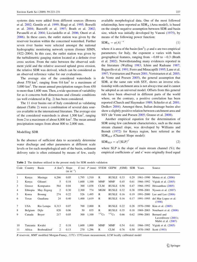
The 11 river basins out of Italy considered as validating
dataset (Table 2) were a combination of several data sour-
ces available in the international literature. The average size
of the considered watersheds is about 1,500 km2, ranging
from 2 to a maximum of about 8,000 km2. The mean annual
precipitation ranges from about 800 to 2,000 mm.
Modelling SDR
In the absence of sufficient data to accurately determine
water discharge and other parameters at different scale
levels or for each morphological unit of the basin, sediment
delivery ratio is often estimated by means of few, easily
available morphological data. One of the most followed
relationship, here reported as SDRA (Area model), is based
on the simple negative assumption between SDR and basin
size, which was initially developed by Vanoni (1975), by
means of the following power function:
SDRA ¼ u Að Þ�j ð1Þ
where A is area of the basin (km2); u and j are two empirical
parameters; for Italy, the exponent j varies with basin
geographical features, ranging from -0.69 to -0.3 (Brath
et al. 2002). Notwithstanding many evidences reported in
the literature (Walling 1983; Ichim and Radoane 1987;
Bagarello et al. 1991; Ferro and Minacapilli 1995; Lane et al.
1997; Verstraeten and Poesen 2001; Vertstraeten et al. 2003;
de Vente and Poesen 2005), the general assumption that
SDR, at the same rate with SSY, shows an inverse rela-
tionship with catchment area is not always true and it cannot
be adopted as an universal model. Offsets from this general
rule have been observed in different parts of the world
where, on the contrary, a positive correlation has been
reported (Church and Slaymaker 1989; Schiefer et al. 2001;
Dedkov 2004). Amongst these, Italian drainage basins also
show a slightly positive relation between catchment area and
SSY (de Vente and Poesen 2005; Grauso et al. 2008).
Another empirical equation for the determination of
SDR using few catchment characteristics, such as the main
stream channel slope, was developed by Williams and
Berndt (1972) for Kenya region, here referred as the
SDRSLP (Channel Slope model):
SDRSLP ¼ u0 SLPð Þj0
ð2Þ
where SLP is the slope of main stream channel (%); the
empirical coefficients u0 and j0 were originally fixed equal
Table 2 The database utilized in the present study for SDR models validation
Code Country Basin A (km2) Slope
(m m-1)
E (m) P (mm) SYEM GEPM f(SMI) SDR Years Source
1 Kenya Masinga 6,266 0.05 1,795 1,510 R RUSLE 0.33 0.29 1961–1990 Mutua et al. (2006)
2 Kenya Gikuuri 5 0.18 1,600 1,100 MMF MMF 0.45 0.61 1966–1992 Vigiak et al. (2005)
3 Greece Kompsatos 564 0.04 300 1,038 CLM RUSLE 0.58 0.47 1966–1992 Hrissanthou (2005)
4 Ethiopia May Zegzeg 2 0.30 2,300 774 MGM RUSLE 0.32 0.38 1998–2001 Nyssen et al. (2007)
5 Korea Bosung 274 0.22 526 1,495 R RUSLE 0.16 0.19 1991–2000 Lee and Lee (2006)
6 Texas Guadiana 24 0.40 1,400 1,619 R RUSLE 0.16 0.17 1991–1995 del Mar Lopez et al.
(1998)
7 USA Rio Lempa 8,313 0.07 700 2,000 R RUSLE 0.22 0.28 1970–1980 Kim et al. (2005)
8 Belgium Dijle 820 0.06 50 835 R RUSLE 0.35 0.18 1969–2003 Notebaert et al. (2008)
9 Canada Boyer 217 0.05 300 1,100 137Cs 137Cs 0.66 0.62 1996–2001 Bernard and
Laverdiwere (2001);
Mabit et al. (2007)
10 Tanzania Kwalei 2 0.18 1,600 1,000 MMF MMF 0.54 0.61 1966–1992 Vigiak et al. (2005)
11 Africa Bosboukloof 2 0.13 270 1,296 R CLM 0.76 0.50 1970–1985 Scott (1993)
R reservoir, MMF modified Morgan-Finney, 137Cs 137Cesium measurement, LCM locally calibrated model
Environ Earth Sci (2009) 59:223–231 227
123
to 0.627 and 0.403, respectively. A different combined
function of catchment area, land slope and land cover, was
used by Kothyari and Jain (1997) for estimating SDR in
India. Unlike the above Areal Model, the Channel Slope-
based Model has been little applied. Moreover, given the
observed very low correlation between the main stream
channel slope parameter utilized in this model and the SDR
data in the Italian basins here considered (r2 = 0.03), SLP
was here replaced with the basin areal mean slope, holding
a stronger link with SDR (r2 = 0.41). Thus, the Slope
model (SDRSlope) relationship was expressed as:
SDRSlope ¼ u Slopeð Þj ð2aÞ
where the mean basin slope is expressed in m 9 m-1 and
u and j are the empirical coefficients to be calibrated on
observed data. As it will be pointed out here, j actually
assumes a negative sign.
In the present study, a new model, the SDRSIM
(Spatially Invariant Model), is proposed, based on a hydro-
morphological function f(SIM) aimed to synthesize in an
unique formulation the roles played both by watershed
morphology and by rainfall amount:
SDRSIM ¼ u � f SMIð Þ�j ð3Þ
with
f SMIð Þ ¼ffiffiffi
Ap
X�ffiffiffiffi
Ep� �
� Slopea
ffiffiffi
Pp
" #
ð3aÞ
where A is the basin area (km2); E is the average elevation
of the basin (m); Slope is the mean basin slope (m 9 m-1);
P is the annual average precipitation amount (mm); and u,
j, X and a are four empirical parameters.
In order to better explain the significance of the factors
combined in Eq. 3a, the single terms that summarize the
SDR can be reformulated as follows: let us consider f(SY)
as a function of the sediment yield, and f(GE) as a function
of the gross erosion in the watershed; then, following the
general empirical assumption that erosion and sediment
yield are influenced by precipitation and climate factors as
well as by basin area, elevation and morphology (Cooke
and Doornkamp 1990; Ludwig and Probst 1998), it may be
written, respectively:
f SYð Þ ¼ Av � Pd � Slopeb ð4Þ
and
f GEð Þ ¼ A# � Pg � Em � Slopec ð5Þ
Reassembling the terms, the SDR equation becomes:
SDR ¼ f SYð Þf GEð Þ ¼
Av � Pd � Slopeb
A# � Pg � Em � Slopec ð6Þ
where the area-rain-slope product function at numerator
represents the final sediment delivery at the basin outlet,
whilst the product-set at denominator drives the soil
mobilization process function and approximates the
watershed gross erosion.
In dimensional terms, Eq. 6 is equivalent to Eq. 3, in
particular, they coincide in the hypothesis that the expo-
nents are such that:
v� # ¼ � j2
; d� g ¼ j2
; b� c ¼ �a; m ¼ 1
2
whilst u = j = 1.
The empirical parameters of each SDR model were
determined using the calibration data set (Table 1). Basi-
cally, the parameter values were estimated against SDRSIM
estimates using a solver that minimized the square error of
estimate. An iterative calibration process was employed for
Eq. 3. First, the set of parameters was approached for f(SY)
and f(GE) functions (Eqs. 4 and 5, respectively). Succes-
sively, Eq. 6 was transformed into model (3), fitting the
SDRSIM values keeping constant some parameters of Eq. 5.
Next, the parameters of Eq. 3 were calibrated against the
SDRSIM estimates. The process was reiterated until a
converging solution was reached.
Models application and results
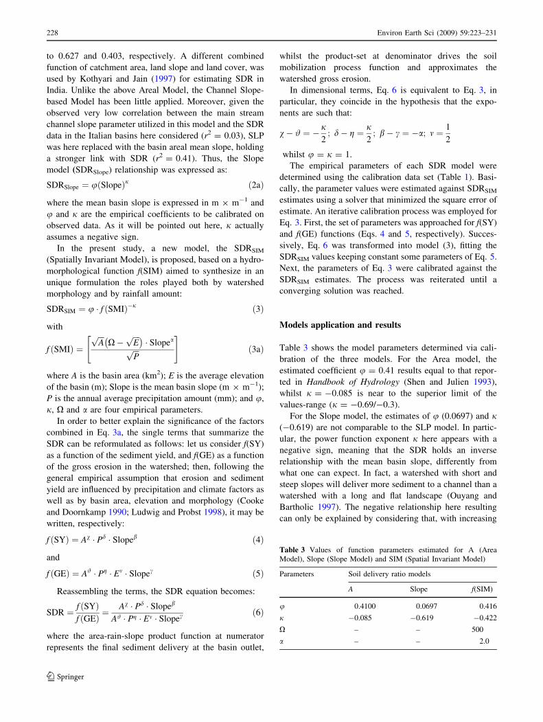
Table 3 shows the model parameters determined via cali-
bration of the three models. For the Area model, the
estimated coefficient u = 0.41 results equal to that repor-
ted in Handbook of Hydrology (Shen and Julien 1993),
whilst j = -0.085 is near to the superior limit of the
values-range (j = -0.69/-0.3).
For the Slope model, the estimates of u (0.0697) and j(-0.619) are not comparable to the SLP model. In partic-
ular, the power function exponent j here appears with a
negative sign, meaning that the SDR holds an inverse
relationship with the mean basin slope, differently from
what one can expect. In fact, a watershed with short and
steep slopes will deliver more sediment to a channel than a
watershed with a long and flat landscape (Ouyang and
Bartholic 1997). The negative relationship here resulting
can only be explained by considering that, with increasing
Table 3 Values of function parameters estimated for A (Area
Model), Slope (Slope Model) and SIM (Spatial Invariant Model)
Parameters Soil delivery ratio models
A Slope f(SIM)
u 0.4100 0.0697 0.416
j -0.085 -0.619 -0.422
X – – 500
a – – 2.0
228 Environ Earth Sci (2009) 59:223–231
123
mean slope, the upland erosion also increases, then, a
surplus of sediment is moved from the valley sides to
channels which cannot be delivered towards the outlet. In
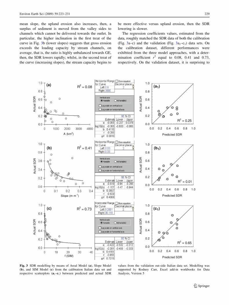
particular, the higher inclination in the first treat of the
curve in Fig. 3b (lower slopes) suggests that gross erosion
exceeds the loading capacity by stream channels, on
average, that is, the ratio is highly unbalanced towards GE,
then, the SDR lowers rapidly; whilst, in the second treat of
the curve (increasing slopes), the stream capacity begins to
be more effective versus upland erosion, then the SDR
lowering is slower.
The regression coefficients values, estimated from the
data, roughly matched the SDR data of both the calibration
(Fig. 3a–c) and the validation (Fig. 3a1–c1) data sets. On
the calibration dataset, different performances were
exhibited from the three model approaches, with a deter-
mination coefficient r2 equal to 0.08, 0.41 and 0.73,
respectively. On the validation dataset, it is surprising to
0.0
0.2
0.4
0.6
0.8
1.0
0.0 0.2 0.4 0.6 0.8 1.0
Predicted SDR
Act
ual S
DR
0.0
0.2
0.4
0.6
0.8
1.0
0.0 0.2 0.4 0.6 0.8 1.0
Predicted SDR
Act
ual S
DR
0.0
0.2
0.4
0.6
0.8
1.0
0.0 0.2 0.4 0.6 0.8 1.0
Predicted SDR
Act
ual S
DR
(c1)
(a1)
(b1)
(c)
(a)
(b)
Act
ual S
DR
Act
ual S
DR
Act
ual S
DR
f (SIM)
Slope (m m-1)
A (km2)
R2 = 0.25
R2 = 0.01
R2 = 0.65
R2 = 0.73
R2 = 0.41
R2 = 0.08
Fig. 3 SDR modelling by means of Areal Model (a), Slope Model
(b), and SIM Model (c) from the calibration Italian data set and
respective scatterplots (a1–c1) between predicted and actual SDR
values from the validation out-side Italian data set. Modelling was
supported by Rodney Carr, Excel add-in workbooks for Data
Analysis, Version 5
Environ Earth Sci (2009) 59:223–231 229
123

detect as only the SIM-model holds the performance, with
r2 = 0.65. With the two simplified Area-and-Slope models,
both validation scatterplots show, in fact, a rather poor
agreement between estimated and actual SDR values, with
a strong decay for the Slope model (Fig. 3b, b1).
The SIM-model may appear more sensitive to variation
in its several parameters than the A and Slope models are to
their few parameters. The application of the SIM model to
other world sites may therefore be limited by the ability
to provide appropriate site-representative parameters able
to capture the spatial variability of SDR data. Specific
geographical locations (e.g., upland and forested basin,
very impermeable drainage areas) may have particular
characteristics which cause the parameters to deviate from
reference values, and may require local optimization.
Conclusions
The effort made hitherto by many researchers to find out a
general model allowing to reliably estimate SDR have
produced a number of different kinds of models, giving to
each the possibility to choose the better solution to his case,
mainly on the basis of actual data availability.
The SDRSIM model here proposed attempted both to
provide a simple method based on easily available catch-
ment parameters and to skip over the limitations observed
when applying other simplified models such as the Areal
model and the Slope model. An integrated hydro-mor-
phological function f(SMI) was introduced, aimed to
synthesize in an unique formulation the roles played both
by watershed morphology and by rainfall amount.
The comparison with the above cited models, through
the application to a wide range of catchments extensions
across different landscapes of Italy, demonstrated the better
behaviour of the proposed model. The validation test per-
formed by means of a 11 basins dataset sparse over
different regions of the world, confirmed the effectiveness
of SDRSIM model against the worse results by the other
models and also proved the model robustness indepen-
dently from the geographic location and local conditions.
Acknowledgments We are grateful to Dr. A. Pagano (EC Joint
Research Centre, IPSC, Ispra) for his suggestions in model mathe-
matics and Dr. G. Fattoruso (ENEA, Portici) for her help in basins
delineation and parameterisation.
References
Arnold JG, Williams JR, Srinivasan R, King KW (1996) The soil and
water assessment tool (SWAT) User’s Manual. Temple, TX
Asselman NEM, Middelkoop H, Dijk PM (2003) The impact of
change in climate and land use on soil erosion, transport and
deposition of suspended sediment in the River Rhine. Hydrol
Process 17:3225–3244
Bagarello V, Ferro V, Giordano G (1991) Contributo alla valutazione
del fattore di deflusso di Williams e del coefficiente di resa solida
per alcuni bacini idrografici siciliani (Evaluation of the Wil-
liams’s runoff factor and of sediment delivery ratio in some
Sicilian river basins). Rivista di Ing Agr 4:238–251
Bazzoffi P, Pellegrini S, Chisci G, Papini R, Scagnozzi A (1997)
Erosione e deflussi a scala parcellare e di bacino in suoli argillosi
a diversa utilizzazione nella val d’Era (Plot and catchment runoff
and erosion in clayey soils of Val d’Era, Tuscany). Agricoltura
Ricerca XVIII(170):5–20
Bernard C, Laverdiwere MC (2001) Assessment of soil erosion at the
watershed scale from 137Cs measurements. In: Stott RH, Mothar
RH, Steinhardt GC (eds) Sustaining the global farm. USDA-
ARS, USA, pp 1034–1038
Biagi B, Chisci G, Filippi N, Missere D, Preti D (1995) Impatto
dell’uso agricolo del suolo sul dissesto idrogeologico. Area
pilota collina cesenate (Influence of cultivations on hydrogeo-
logical equilibrium of soils). Collana Studi e Ricerche, Regione
Emilia Romagna, Assessorato Agricoltura, Bologna, Italy, 153
pp
Bonora N, Immordino F, Schiavi C, Simeoni U, Valpreda E (2002)
Interaction between catchment basin management and coastal
evolution (Southern Italy). J Coast Res SI 36:81–88
Borselli L, Cassi P, Sanchis PS, Ungaro F (2004) Studio della
dinamica delle aree sorgenti primarie di sedimento nell’area
pilota del Bacino di Bilancino (Primary sediment sources in the
Bilancino reservoir watershed area): BABI Project. Report of the
Consiglio Nazionale delle Ricerche. Istituto di Ricerca per la
Protezione Idrogeologica (CNR-IRPI), Florence Unit, «Pedolo-
gia Applicata», pp 104
Brath A, Castellarin A, Montanari A (2002) Assessing the effect of
land-use changes on annual average gross erosion. Hydrol Earth
Syst Sci 6:255–265
Church M, Slaymaker O (1989) Disequilibrium of Holocene sediment
yield in glaciated British Columbia. Nature 337:452–454
Collins AL, Walling DE (2004) Documenting catchment suspended
sediment sources: problems, approaches and prospects. Prog
Phys Geogr 28(2):159–196
Cooke RU, Doornkamp JC (1990) Geomorphology in environmental
management. Clarendon Press, Oxford, p 79
de Vente J, Poesen J (2005) Predicting soil erosion and sediment yield
at the basin scale: scale issues and semi-quantitative models.
Earth Sci Rev 71:95–125
Dedkov A (2004) The relationship between sediment yield and
drainage basin area. In: Sediment transfer through the fluvial
system, vol 288 (Proceedings of a symposium held in Moscow,
August 2004), IAHS Publishing, USA, pp 197–204
del Mar Lopez T, Mitchell Aide T, Scatena FN (1998) The effect of
land use on soil erosion in the Guadiana watershed in Puerto
Rico. Carib J Sci 34(3–4):298–307
Fan JR, Zhang JH, Zhong XH, Liu SZ (2004) Monitoring of soil
erosion and assessment for contribution of sediments to rivers in
a typical watershed of the upper Yangtze river basin. Land
Degrad Dev 15:411–421
Ferro V, Minacapilli M (1995) Sediment delivery processes at basin
scale. Hydrol Sci J 40:703–717
Gentile F, Puglisi S, Trisorio-Liuzzi G (1999) Verifica sperimentale di
modelli empirici per la valutazione della perdita di suolo in un
piccolo bacino molisano (Experimental test of empirical models
for soil loss assessment in a small catchment). Proceedings: La
Gestione dell’Erosione: il controllo dei fenomeni torrentizi,
scienza, tecnica e strumenti. Quaderni di Idronomia Montana
19/1, BIOS Edition, pp 103–117
230 Environ Earth Sci (2009) 59:223–231
123
Grauso S, De Bonis P, Fattoruso G, Onori F, Pagano A, Regina P,
Tebano C (2008) Relations between climatic-geomorphological
parameters and suspended sediment yield in a Mediterranean
semi-arid area (Sicily, southern Italy). Env Geol 54:219–234
Hrissanthou V (2005) Estimate of sediment yield in a basin without
sediment data. Catena 64:333–347
Ichim I, Radoane M (1987) A multivariate statistical analysis of
sediment yield and prediction in Romania. In: Ahnert F (ed)
Geomorphological models: theoretical and empirical aspects.
Catena Suppl 10:137–146
Kim BJ, Saunders P, Finn JT (2005) Rapid assessment of soil erosion
in the Rio Lempa Basin, Central America, using the universal
soil loss equation and geographic information systems. Environ
Manage 36(6):872–885
Kothyari UC, Jain SK (1997) Sediment yield estimation using GIS.
Hydrol Sci J 42:833–843
Lane JL, Hernandez M, Nichols M (1997) Processes controlling
sediment yield from watersheds as functions of spatial scale.
Environ Modell Softw 12(4):355–369
Lee GS, Lee KH (2006) Scaling effect for estimating soil loss in the
RUSLE model using remotely sensed geospatial data in Korea.
Hydrol Earth Syst Discussion 3:135–157
Lenhart T, Van Rompaey A, Steegen A, Fohrer N, Frede HG, Govers
G (2005) Considering spatial distribution and deposition of
sediment in lumped and semi-distributed models. Hydrol Process
19(3):785–794
Licciardello F, Mazzola G, Zema DA, Zimbone SM (2006) Runoff
and soil erosion modelling by ANNAGNPS in a small Mediter-
ranean watershed. Proceedings of the 5th Iberian Congress on
‘‘Water Management and Planning’’. Faro, Algarve, Portugal,
04–08 December
Lionello P, Malanotte-Rizzoli P, Boscolo R, Alpert V, Li L,
Luterbacher J, May W, Trigo R, Tsimplis M, Ulbrich U,
Xoplaki E (2006) The Mediterranean climate: an overview of the
main characteristics and issues. In: Lionello P et al (eds)
Mediterranean climate variability. Elsevier, Amsterdam, pp 1–25
Lu H, Morana C, Prossera I, Sivapalan M (2004) Modelling sediment
delivery ratio based on physical principles. In: Proceedings
iEMS 2004 International Conference, 14–17 June 2004, Univer-
sity of Osnabruck, Germany, http://www.iemss.org/iemss2004/
Ludwig W, Probst JL (1998) River sediment discharge to the oceans:
present-day controls and global budgets. Am J Sci 298:265–295
Mabit L, Bernard C, Laverdiere MR (2007) Assessment of erosion in
the Boyer River watershed (Canada) using GIs iruented sampling
strategy and 137Cs measurements. Catena 71:242–249
Mutchler CK, Murphree CE, Mcgregor KC (1994) Laboratory and
field plots for erosion research. In: Lal S (ed) Soil erosion.
Research method. CRC Press, USA, pp 11–38
Mutua BM, Klik A, Loiskandl W (2006) Modelling soil erosion and
sediment yield at a catchment scale: the case of Masinga
catchment, Kenya. Land Degrad Dev 17(5):557–570
Notebaert B, Verstraeten G, Govers G, Poesen J (2008) Qualitative
and quantitative applications of LiDAR imagery in fluvial
geomorphology. Earth Surf Process Landforms (in Press)
Nyssen J, Poesen J, Moeyersons J, Haile M, Deckers J (2007)
Dynamics of soil erosion rates and controlling factors in the
Northern Ethiopian Highlands—towards a sediment budgets.
Earth Surf Process Landforms 33(5):695–711
Onori F, De Bonis P, Grauso S (2006) Soil erosion prediction at the
basin scale using the revised universal soil loss equation
(RUSLE) in a catchment of Sicily (southern Italy). Environ
Geol 50(9):1129–1140
Ouyang D, Bartholic J (1997) Predicting sediment delivery ratio in
Saginaw Bay watershed. 22nd National Association of Environ-
mental Professionals Conference Proceedings. 19–23 May 1997,
Orlando, pp 659–671
Pavanelli D, Pagliarani A, Bigi A (2004) Monitoraggio idrotorbid-
imetrico per la stima dell’erosione nel bacino montano del Reno
(Sediment yield monitoring for erosion estimate in the river
Reno watershed). Suppl ARPA J 6:3–7
Schiefer E, Slaymaker O, Klinkenberg B (2001) Physiographically
controlled allometry of specific sediment yield in the Canadian
cordillera: a lake sediment-based approach. Geogr Ann 83:55–65
Scott DF (1993) The hydrological effects of fire in South African
mountain catchments. J Hydrol 150:409–432
Shen HW, Julien PY (1993) Erosion and sediment transport In:
Maidment DR (ed) Handbook of Hydrology, Chap 12. McGraw-
Hill, New York
Van Rompaey AJJ, Bazzoffi P, Jones RJA, Montanarella L, Govers G
(2003) Validation soil erosion risk assessment in Italy. European
Soil Bureau Research Report No. 12, EUR 20676 EN, 25 pp
Vanoni VA (1975) Sediment deposition engineering. ASCE Manuals
and Reports on Engineering Practices, p 54
Verstraeten G, Poesen J (2001) Factors controlling sediment yield
from small intensively cultivated catchments in a temperate
humid climate. Geomorphology 40:123–144
Vertstraeten G, Poesen J, de Vente J, Koninckx X (2003) Sediment
yield variability in Spain: a quantitative and semiqualitative
analysis using reservoir sedimentation rates. Geomorphology
50:327–348
Vigiak O, Okoba BO, Sterk G, Stroosnijder L (2005) Water erosion
assessment using farmers’ indicators in the West Usambara
Mountains, Tanzania. Catena 64:307–320
Walling DE (1983) The sediment delivery problem. J Hydrol 65:209–
237
Williams JR, Berndt HD (1972) Sediment yield computed with
Universal equation. J Hydraulic Div ASCE98 (HY2), pp 2087–
2098
Wolman MG (1977) Changing needs and opportunities in the
sediment field. Water Resour Res 13(1):50–54
Environ Earth Sci (2009) 59:223–231 231
123