Embed Size (px)
Citation preview
ELSEVIER
DISCRETE APPLIED
Discrete Applied Mathematics 66 ( 1996) 8 l-94 MATHEMATICS
Note
An improved lower bound for the bin packing
Department of Managemenr and Systems, College of Business and Economics, Washington State University,
Pullman, WA 99164-4726, USA
h Department of Management, Marquette University, PO. Box 1881, Milwaukee, WI 53201-1881. USA
Received 14 October 1994; revised 1 August 1995
Abstract
This paper unifies and generalizes the existing lower bounds for the one-dimensional bin packing problem. The generalization is motivated by and based on the work of Martello and Toth (this journal, 1990). The worst-case performance of the unified lower bound is analyzed and two new lower bounds are proposed and compared with existing lower bounds through numeric31 experiments.
Keywords: Bin packing problem; Lower bound; Worst-case analysis
1. Introduction
In this paper we present an extension of the results of Martello and Toth [4], for
computing lower bounds for the bin packing problem (BPP) . Formally, the BPP problem
can be stated as follows:
Given a set I = {l,... ,n} of n items, each having a positive integer size si,
pack the items of I into a minimum number of bins, each of capacity C > si
(i=l,...,n).
One of the most extensively studied combinatorial problems, BPP has a wide range
of practical applications such as in storage allocation, cutting stock [ 61, multiprocessor
scheduling [ 11, and loading in flexible manufacturing systems [ 31 (for an excellent
review of BPP see [ 1 ] ). Since the problem is NP-hard in the strong sense [ 21, most
* Corresponding author. E-mail: [email protected].
0166-218X/96/$15.00 @ 1996 Elsevier Science B.V. All rights reserved
SSDfOl66-2lSX(9S)OOlO8-5
82 B. Chen, B. Srivastava/Discrete Applied Mathematics 66 (1996) 81-94
research has centered on the development of heuristic algorithms and characterizing their
worst-case performance relative to the optimal packing. Little work has been reported
on the development of lower bounds and exact algorithms for BPP (see [4] ). In this
paper, we develop a new procedure to compute lower bounds for BPP by generalizing
and extending the idea presented in [4]. Under different parameter settings, the new
procedure generates two existing lower bounds, and two new and better lower bounds.
The paper is organized as follows. Section 2 introduces a unified lower bound for
BPP and analyzes its worst-case performance. Section 3 presents an improved lower
bound by incorporating a search procedure. In Section 4 we develop efficient procedures
to compute the key elements of the unified lower bound. Finally, in Section 5 we report
results for several numerical experiments for the unified lower bound under different
parameter settings. In the rest of the paper we assume, without loss of generality, that
the II items in I are sorted according to their size such that
s1 3 s2 3 . . . > S”. (1)
2. A unified lower bound
For 0 6 a < b < 1, let I( a, b] denote the set of items such that aC < si 6 bC and
N( a, b] denote the minimum number of bins (each of capacity C) required to pack
the items in set Z(a, b]. In a similar fashion Z[a, b] and N[a, b] are defined. Clearly,
N[O, l] is the value of the optimal solution of BPP
Let m be a positive integer. Define
Since N( 1 , 1 ] = 0 by definition, Lr reduces to [CiEI si/C] and L, can then be written
as:
L, =max{N(l/m, ll,h}. (2)
Lemma 2.1. L,, is a valid lower bound for BPP for any positive integer m and
L rn+l 2 L,,.
Proof. It is well known that L1 is the continuous relaxation of BPP. Further N( l/m, l]
is also a lower bound for BPP, since it is the minimum number of bins required to pack
items in I( l/m, l] C I. It follows that L,, is a lower bound. The second part of the
lemma is obvious since Z(l/m, I] & I( l/(m+ l), 11. 0
In general, N( l/m, l] and thus L, is difficult to compute except for small values
of m. Indeed, L, includes two existing lower bounds as special cases. For m = 1, L,
reduces to the classical continuous relaxation bound, and for m = 2, it reduces to the
B. Chen, B. Srivastava/Discrete Applied Mathematics 66 (1996) 81-94 83
lower bound proposed in [4]. Later in this paper, we will develop efficient procedures
to compute L3 and a lower bound on L4 (better than L3) .
To
Lemma 2.2. For any positive integer m, we have
L,, m m-2 1
N[O,l] 3 --- m-t1 m+ 1 NO, 11 (3)
and the inequality is tight for at least one instance of BPP
Proof. Given any positive integer m, a feasible solution based on L, can be constructed
as follows. First, assign all items in I( l/m, l] to N( l/m, l] bins in an optimal fashion.
Next, assign each of the items in I[O, l/m] to an already initialized bin or to a new
bin, when the current item does not fit in any of the already opened bins. If all items
in I [ 0,l /ml were divisible, then L,, bins would be sufficient for the above assignment
(by definition of L,) Further, no more than L, - 1 items in I [ 0,l /ml need to be split
between different bins. Therefore, to construct a feasible solution, it suffices to reassign
the split items. Since si < C/m for all i E I [ 0,l /ml by definition, only I( L,, - 1 )/ml
additional bins are required. Thus, the number of bins used by this procedure to pack
all n items of I is no more than
L,, + [(L, - 1)/m] 6 L, + CL, - 1)/m+ Cm - 1)/m m-2 2Q,+-
m m .
It follows that
m+l m-2 --L,, + m - 3 NEO, 11
m
and the desired inequality is obtained by rearranging terms.
To show that the inequality is tight for any positive integer m, consider an instance
of BPP for which C = n = 2m + 1, si = 2 for all i E 1. The value of the optimal
solution N[O, l] for this instance is [n/ml = 3 and the lower bound L,, = [ns;/Cl = 2.
Substituting L,, and N[O, l] into the inequality, one can verify that it is tight. 0
Theorem 2.3. W( L1) = l/2 and W( L,) = 213 for any integer m > 2.
84
Table 1
B. Chen, B. Srivastava/Discrete Applied Mathematics 66 (1996) 81-94
NO, 11
112 I 2 3 4 5 6 cc 1 I 1 0.667 0.625 0.600 0.583 l/2
2 1 1 0.667 0.667 0.667 0.667 213
3 1 1 0.667 0.688 0.700 0.708 314
4 1 1 0.667 0.700 0.720 0.733 415
5 1 1 0.667 0.708 0.733 0.750 516
‘.
03 1 1 213 314 415 516 . . 1
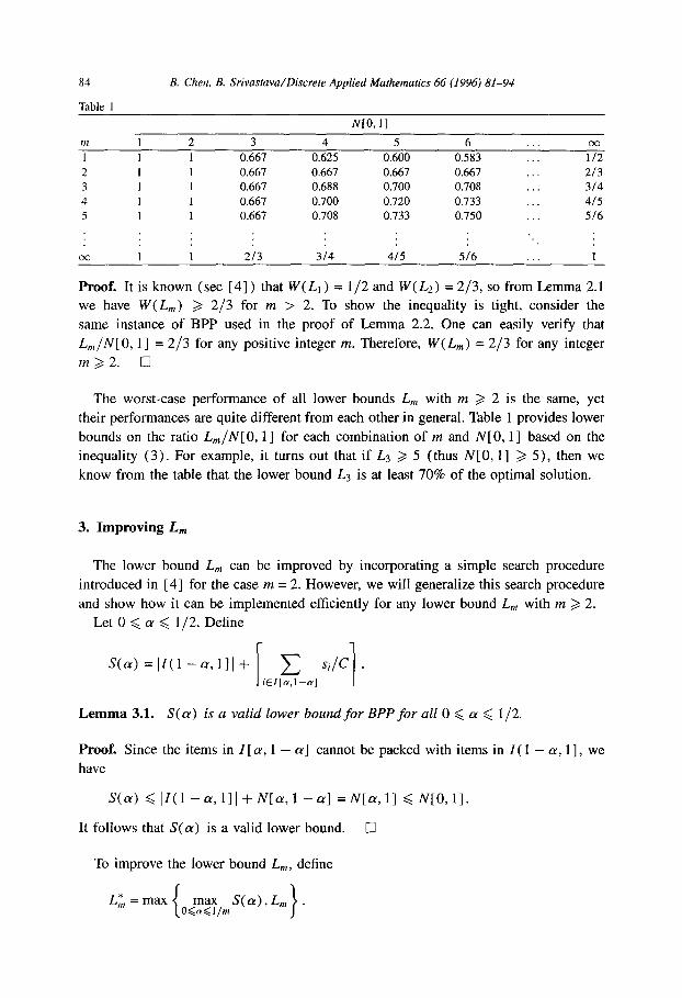
Proof. It is known (see [ 41) that W( Li ) = l/2 and W( L2) = 2/3, so from Lemma 2.1
we have W( L,) 2 2/3 for m > 2. To show the inequality is tight, consider the
same instance of BPP used in the proof of Lemma 2.2. One can easily verify that
L,,/N[O, l] = 2/3 for any positive integer m. Therefore, W( L,,) = 2/3 for any integer
m>2. 0
The worst-case performance of all lower bounds L, with m 2 2 is the same, yet
their performances are quite different from each other in general. Table 1 provides lower
bounds on the ratio L,/N[O, l] for each combination of m and N[ 0, 11 based on the
inequality (3). For example, it turns out that if Ls 3 5 (thus N[O, l] > 5), then we
know from the table that the lower bound L3 is at least 70% of the optimal solution.
3. Improving L,
The lower bound L, can be improved by incorporating a simple search procedure
introduced in [4] for the case m = 2. However, we will generalize this search procedure
and show how it can be implemented efficiently for any lower bound L, with m 3 2.
Let 0 6 CY < l/2. Define
S(a) =]Z(l-a,llI+ [iEIg-cx] si’cl .
Lemma 3.1. S(a) is a valid lower bound for BPP for all 0 < cx < l/2.
Proof. Since the items in I [ a, 1 - cu] cannot be packed with items in Z( 1 - (Y, 11, we
have
S(a) < lZ(l-a,ll]+N[a,l-o] =N[LY,l] <N[O,l].
It follows that S(cu) is a valid lower bound. 0
To improve the lower bound L,, define
L,T, = max {
max S(a), L, . O<CX<l/tit >
B. Chen, B. Srivastava/Discrete Applied Mathematics 66 (1996) 81-94 85
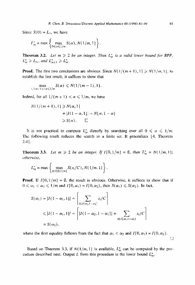
Since S(0) = Lr, we have
L,T, = max 1
O<m~,n,S(~),N(l/m, 11 . \a.. 1
Theorem 3.2. Let m > 2 be an integer. Then L,*, is a valid lower bound for BPP,
L,T, 3 L,,, , and Li,,, 3 Li,.
Proof. The first two conclusions are obvious. Since N( 1 /(m + 1) , 1 ] 2 N( 1 /m, I], to
establish the last result, it suffices to show that
Indeed, for all l/(m+ 1) < (Y 6 l/m, we have
N(l/(m+l),ll bN(Gll
=(1(1-cu,l]I+N[(Y,l-~]
>S((Y). 0
It is not practical to compute L,T, directly by searching over all 0 < cy < l/m.
The following result reduces the search to a finite set. It generalizes [4, Theorem
2.41.
Theorem 3.3. Let m >/ 2 be an integer. If I [ 0,1/m] = 0, then Lz, = N( l/m, 1 ] ;
otherwise,
L,:, = max
Proof. If I [0,1/m] = 8, the result is obvious. Otherwise, it suffices to show that if
0 < ai < LYE 6 l/m and Z[o,(~r) = I[O,al), then S(ar) < S(W). In fact,
S(cul) = (I(1 -W,llIi- (;El[Z-a,l si’cl
<II(l-ai,llJf Il(l-~2,l--(y1ll+
/ = /1 Si C
iEl[az.l-al
= S(a2),
where the first equality follows from the fact that (~1 < (~2 and I [ 0, ar ) = I [ 0, cu2).
q
Based on Theorem 3.3, if N( l/m, l] is available, Lz, can be computed by the pro-
cedure described next. Output L from this procedure is the lower bound Lz,.
86 B. Chen, B. Srivastava/Discrete Applied Mathematics 66 (1996) 81-94
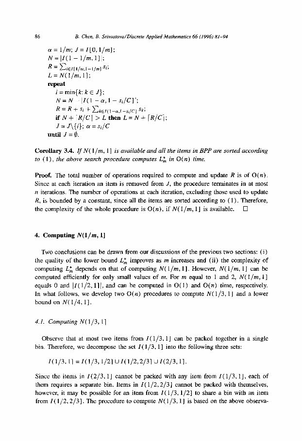
(Y = l/m; .z = Z[O, l/m]; N= ]Z(l - l/m,l]l;
R = CiEl,l,rn,l--l,m, si; L=N(l/m,l]; repeat
i = min{k: k E J};
N=N-IZ(l-cr,l-si/C]I; R=R+si+C kEI(l-al-s;/C] sk;
if N+ [R/Cl > L then L=N+ [R/C];
J = J\(i); Ly = si/C
until J = 0.
Corollary 3.4. If N ( 1 /m, 1 ] is available and all the items in BPP are sorted according
to ( 1) , the above search procedure computes LG in O(n) time,
Proof. The total number of operations required to compute and update R is of O(n).
Since at each iteration an item is removed from J, the procedure terminates in at most n iterations. The number of operations at each iteration, excluding those used to update R, is bounded by a constant, since all the items are sorted according to ( 1) . Therefore, the complexity of the whole procedure is O(n), if N( l/m, l] is available. 0
4. Computing N(l/m, l]
Two conclusions can be drawn from our discussions of the previous two sections: (i) the quality of the lower bound LG improves as m increases and (ii) the complexity of computing L;, depends on that of computing N( l/m, 11. However, N( l/m, 11 can be computed efficiently for only small values of m. For m equal to 1 and 2, N( l/m, 11 equals 0 and IZ( l/2,1] 1, and can be computed in O( 1) and O(n) time, respectively. In what follows, we develop two O(n) procedures to compute N( l/3,1 ] and a lower bound on N( l/4,1].
4.1. Computing N( l/3, l]
Observe that at most two items from Z( l/3,1 ] can be packed together in a single bin. Therefore, we decompose the set Z( l/3, l] into the following three sets:
1(1/3,1] =z(1/3,1/21~z(1/2,2/31~z(2/3,11.
Since the items in Z(2/3, l] cannot be packed with any item from Z( l/3,1], each of them requires a separate bin. Items in Z( l/2,2/3] cannot be packed with themselves, however, it may be possible for an item from Z( l/3, l/2] to share a bin with an item from Z( l/2,2/3]. The procedure to compute N( l/3, l] is based on the above observa-
B. Chen, B. Srivastava/Discrete Applied Mathematics 66 (1996) 81-94 87
tion and the dominance criterion described in [ 41. We briefly describe the dominance
criterion next.
Given any item i E I, the dominance criterion is used to identify the dominant set
B containing i (if it exists), such that there exists an optimal solution in which a bin
contains exactly the items in set B. Once B has been identified, items of B can be
assigned to a bin and removed from further consideration. The dominant set can be
identified by repeatedly checking for dominance between any two distinct and feasible
packings. Martello and Toth [4] have given the following sufficient condition for this
purpose. Given two distinct feasible packings A and B, B dominates A if there exists a
partition {At, . . , Ak} of A and a subset {iI,. . . , ik} of B, such that siP > xjEA, s.j for
p=l,...,k.
The following procedure computes N( l/3,1 1.
I, := I( l/2,2/3]; Z2 := I( l/3,1/2];
1; := 0; 1; := 0;
N := )1(2/3,1] /; LY := l/2;
if I, # 8 and Z2 # 8 then
repeat
i := min{k: k E 12);
12 := Z2 \ {i};
Zi := Zi U I( 1 - Ly, 1 - Si/C];
cl := sJC;
if Zi # 8 then
i’ := min{k: k E Z{};
Zi := Z[ \ {i’};
I1 := II \ {i’};
B := {i, i’};
N:=N+l;
else Zi := Zi U {i};
until (II = 0 or 12 = 0)
IV := A’+ 1111 + [(I121 + (1;1)/‘4.
Theorem 4.1. If all items i E I( l/3, l] are sorted according to ( 1)) the above proce-
dure computes N( l/3, l] correctly in O(n) time.
Proof. The correctness of the above procedure is shown by the following four facts.
(i) If an item i’ E I( l/2,2/3] is packed with an item i E I( l/3,1/2] using the above
procedure, the resulting packing B dominates any other packing containing item i’. This
is because of the fact that item i has the largest size among all the items currently in
12, and by the dominance criterion, B = {i,i’} is contained in some optimal solution.
We can therefore remove items i and i’ from further consideration. (ii) If an item
i E I ( l/3, l/2] is assigned to set I.& then i cannot be packed with any of the items
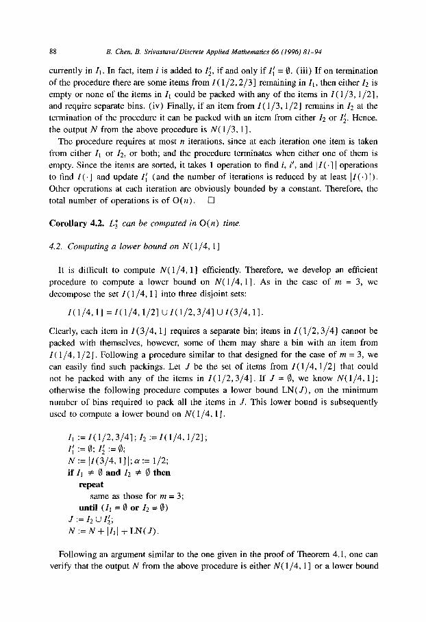
88 B. Chen, B. Srivastava/Discrete Applied Mathematics 66 (1996) 81-94
currently in It. In fact, item i is added to Zi, if and only if Z/ = 8. (iii) If on termination
of the procedure there are some items from I( l/2,2/3] remaining in It, then either 12 is
empty or none of the items in It could be packed with any of the items in I( l/3,1/2],
and require separate bins. (iv) Finally, if an item from I( l/3, l/2] remains in 12 at the
termination of the procedure it can be packed with an item from either Z2 or Z.& Hence,
the output N from the above procedure is N( l/3,1].
The procedure requires at most n iterations, since at each iteration one item is taken
from either It or Z2, or both; and the procedure terminates when either one of them is
empty. Since the items are sorted, it takes 1 operation to find i, i’, and (I( .] ) operations
to find Z ( .] and update Z,l (and the number of iterations is reduced by at least IZ( .) I).
Other operations at each iteration are obviously bounded by a constant. Therefore, the
total number of operations is of O(n). 0
Corollary 4.2. L; can be computed in O(n) time.
4.2. Computing a lower bound on N( l/4,1]
It is difficult to compute N( l/4, l] efficiently. Therefore, we develop an efficient
procedure to compute a lower bound on N( l/4,1 1. As in the case of wz = 3, we
decompose the set I( l/4, I] into three disjoint sets:
Z(1/4,1] =Z(1/4,1/2]uZ(1/2,3/4]uZ(3/4,1].
Clearly, each item in I( 3/4,1] requires a separate bin; items in I( l/2,3/4] cannot be
packed with themselves, however, some of them may share a bin with an item from
I( l/4, l/2]. Following a procedure similar to that designed for the case of m = 3, we
can easily find such packings. Let J be the set of items from I( l/4, l/2] that could
not be packed with any of the items in I( l/2,3/4]. If J = 0, we know N( l/4, I];
otherwise the following procedure computes a lower bound LN( J), on the minimum
number of bins required to pack all the items in J. This lower bound is subsequently
used to compute a lower bound on N( l/4,1].
I, := I( l/2,3/4]; Z2 := I( l/4,1/2];
z; := 0; z; := 0; N := ]Z(3/4, l] I; a := l/2;
if II # 8 and Z2 # 0 then
repeat same as those for m = 3;
until (II = 0 or Z2 = 0) J := 12 u zi; N := N+ [Z,l +LN(.Z).
Following an argument similar to the one given in the proof of Theorem 4.1, one can
verify that the output N from the above procedure is either N( l/4, l] or a lower bound
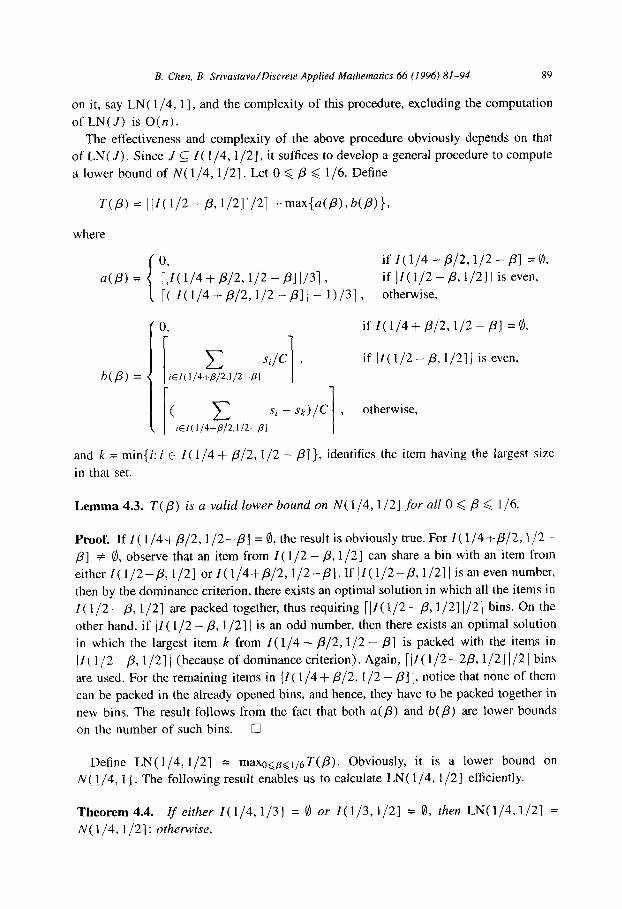
B. Chen, B. Srivastava/Discrete Applied Mathematics 66 (1996) 81-94 89
on it, say LN( l/4, l], and the complexity of this procedure, excluding the computation
of LN(J) is O(n).
The effectiveness and complexity of the above procedure obviously depends on that
of LN( 1). Since J & f ( l/4,1 /2], it suffices to develop a general procedure to compute
a lower bound of N( l/4,1/2]. Let 0 6 p < l/6. Define
T(P) = ~jZ(1/2-p,1/211/21+max{a(~),b(P)),
where
(;iZ(l/4+P,2,1/2-P],/3i,
if I( l/4 + p/2,1/2 - PI = 0, if Jf(1/2--p,1/2]) iseven,
[(lZ(1/4+fl/2,1/2--pl] - 1)/31, otherwise,
ifZ(1/4+p/2,1/2-PJ =0,
c Si/C b(P) = iE1(1/4+p/2.1/2-P1 l3 if )I( l/2 - p, l/21 ] is even,
t c Si -Sk)/C 1 7 otherwise,
i~lC1/4+P/2,1/2-P1
and k = min{i: i E I( l/4 + p/2,1/2 - PI}, identifies the item having the largest size
in that set.
Lemma 4.3. T(P) is a valid lower bound on N( l/4,1 /2] for all 0 < p 6 l/6.
Proof. If I( 1/4+j3/2,1/2-p] = 0, the result is obviously true. For I( 1/4+@/2,1/2-
p] # 0, observe that an item from I( l/2 - /I, l/2] can share a bin with an item from
either I( 1/2-p, l/21 or Z( 1/4+,B/2,1/2-p]. If lZ( 1/2-j?, l/2]] is an even number,
then by the dominance criterion, there exists an optimal solution in which all the items in
I( l/2 - p, l/2] are packed together, thus requiring [\Z( l/2 - p, l/2] l/21 bins. On the
other hand, if IZ( l/2- J3. l/21] is an odd number, then there exists an optimal solution
in which the largest item k from I( l/4 + p/2,1/2 - p] is packed with the items in
lZ(l/2-P,l/211 (b ecause of dominance criterion). Again, [jZ ( l/2 - 2p, l/21 I/21 bins
are used. For the remaining items in (I( l/4+ p/2, l/2 - p] 1, notice that none of them
can be packed in the already opened bins, and hence, they have to be packed together in
new bins. The result follows from the fact that both a(P) and b(P) are lower bounds
on the number of such bins. q
Define LN( l/4,1/2] = maxocpGi/6T(P). Obviously, it is a lower bound on
N( l/4, I]. The following result enables us to calculate LN( l/4, l/2] efficiently.
Theorem 4.4. rf either I( l/4,1/3] = 0 or I( l/3,1/2] = 8, then LN( l/4,1/2] =
N( l/4,1 /2] ; otherwise,
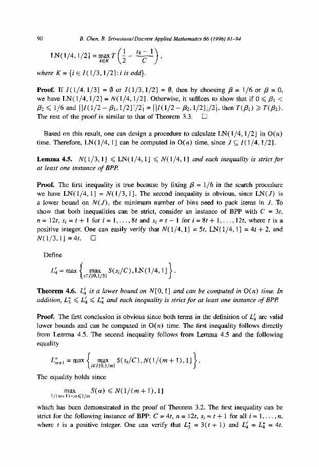
90 B. Chen, B. Srivastava/Discrete Applied Mathematics 66 (1996) 81-94
LN( l/4,1/2] = yEyT (1 ?!$A), z -
whereK={iEZ(1/3,1/2]:iisodd}.
Proof. If I( l/4,1/3] = 0 or I( l/3,1/2] = 0, then by choosing p = l/6 or ~3 = 0,
we have LN( l/4,1/2] = N( l/4,1/2]. Otherwise, it suffices to show that if 0 6 pt <
P2 < l/6 and UZ(l/2 - Pt, l/21 l/4 = W(1/2 - P2,1/21//21, then WI) b T(/W. The rest of the proof is similar to that of Theorem 3.3. 0
Based on this result, one can design a procedure to calculate LN( l/4,1/2] in O(n)
time. Therefore, LN( l/4,1 ] can be computed in O(n) time, since J C I( l/4,1/2].
Lemma 4.5. N( l/3,1 ] 6 LN( l/4,1 ] < N( l/4,1 ] and each inequality is strict for
at least one instance of BPZ?
Proof. The first inequality is true because by fixing p = l/6 in the search procedure
we have LN( l/4, l] = N( l/3,1]. The second inequality is obvious, since LN( .Z) is
a lower bound on N( .Z), the minimum number of bins need to pack items in J. To
show that both inequalities can be strict, consider an instance of BPP with C = 3t,
n=12t,si=t+lfori=l,..., 8tandsi=t--lfori=8t+1,...,12t,wheretisa
positive integer. One can easily verify that N( l/4,1] = 3, LN( l/4,1] = 4t -k 2, and
N( l/3, l] = 4t. 0
Define
Lk=max
Theorem 4.6. Li is a lower bound on N[O, 11 and can be computed in O(n) time. In addition, L; < Li < Lz and each inequality is strict for at least one instance of BPZ?
Proof. The first conclusion is obvious since both terms in the definition of Li are valid
lower bounds and can be computed in O(n) time. The first inequality follows directly
from Lemma 4.5. The second inequality follows from Lemma 4.5 and the following
equality
L* tllfl = max max S(si/C>,N(l/(m+ l), 11 iEI[O.l/ml
The equality holds since
,,c~,+$~~<l,~15(o) < N(l/(m + l), 11 .
which has been demonstrated in the proof of Theorem 3.2. The first inequality can be
strict for the following instance of BPP: C = 4t, n = 12t, si = t + 1 for all i = 1, . . . , n, where t is a positive integer. One can verify that Lz = 3( t + 1) and Li = LT = 4t.
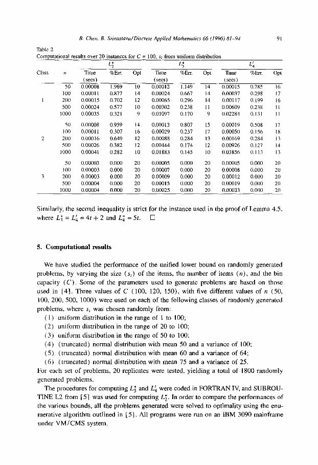
B. Chen, B. Srivastava/Discrete Applied Mathematics 66 (1996) 81-94 91
Table 2
Computational results over 20 instances for C = 100, Si from uniform distribution
L; L; Lk
Class n Time %ElX Opt Time %EIT. Opt Time %Err. Opt
50
(sets) 0.00008 1.969 10
(sea) 0.00012 1.149 14
(sets)
0.00015 0.785 16
100 0.00011 0.877 14 0.00024 0.667 14 0.00037 0.298 17
I 200 0.00015 0.702 12 0.00065 0.296 14 0.00117 0.199 16
500 0.00024 0.577 10 0.00302 0.238 11 0.00609 0.238 1 I 1000 0.00035 0.321 9 0.01097 0.170 9 0.02284 0.131 I1
50 0.00008 0.959 14 0.00013 0.807 15 0.00019 0.508 17
100 0.00011 0.307 16 0.00029 0.237 17 0.00050 0.156 18
2 200 0.00016 0.649 12 0.00088 0.284 13 0.00169 0.284 13
500 0.00026 0.382 12 0.00444 0.174 12 0.00926 0.127 14
1000 0.00041 0.282 10 0.01883 0.145 10 0.03856 0.113 13
SO 0.00003 0.000 20 0.00005 0.000 20 0.00005 0.000 20
100 0.00003 0.000 20 0.00007 0.000 20 0.00008 0.000 20
3 200 0.00003 0.000 20 0.00009 0.000 20 0.00012 0.000 20
500 0.00004 0.000 20 0.00015 0.000 20 0.00019 0.000 20
1000 0.00004 0.000 20 0.00025 0.000 20 0.00033 0.000 20
Similarly, the second inequality is strict for the instance used in the proof of Lemma 4.5,
where L; = Li, = 4t + 2 and Lb” = 5t. 0
5.
92 B. Chen, B. Srivastava/Discrete Applied Mathematics 66 (1996) 81-94
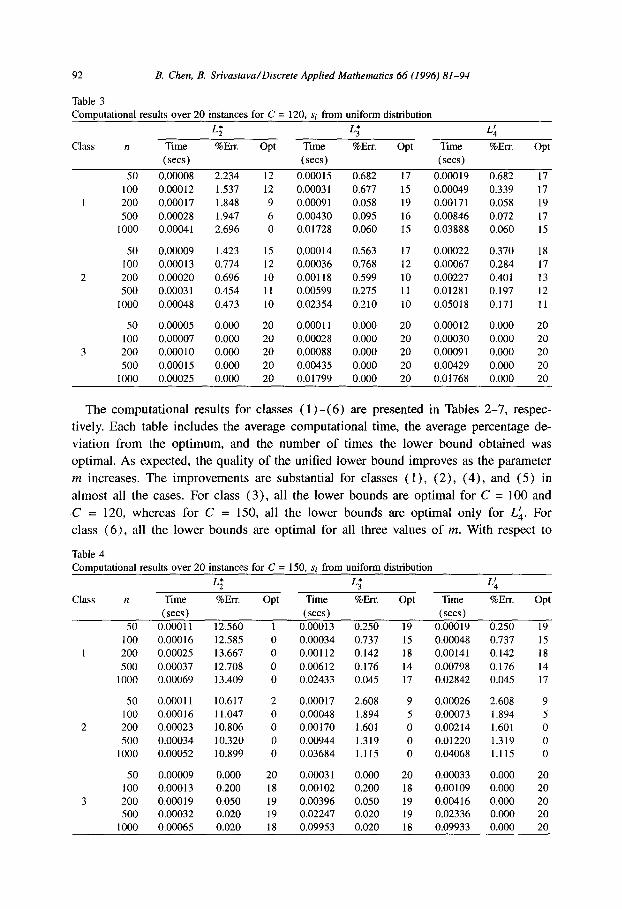
Table 3
Computational results over 20 instances for C = 120, si from uniform distribution
L; L; L:
Class n Time %Err. Opt Time %EIT. Opt Time %Err. Opt (sets) (sets) (sets)
50 0.00008 2.234 12 0.00015 0.682 17 0.00019 0.682 17
100 0.00012 1.537 12 0.0003 1 0.677 15 0.00049 0.339 17
1 200 0.00017 1.848 9 0.00091 0.058 19 0.00171 0.058 19
500 0.00028 1.947 6 0.00430 0.095 16 0.00846 0.072 17
1000 0.00041 2.696 0 0.01728 0.060 15 0.03888 0.060 15
50 0.00009 1.423 15 0.00014 0.563 17 0.00022 0.370 18
100 0.00013 0.774 12 0.00036 0.768 12 0.00067 0.284 17
2 200 0.00020 0.696 10 0.00118 0.599 10 0.00227 0.401 13
500 0.0003 1 0.454 11 0.00599 0.275 11 0.01281 0.197 12
1000 0.00048 0.473 10 0.02354 0.210 10 0.05018 0.171 11
50 0.00005 0.000 20 0.000 11 0.000 20 0.00012 0.000 20
100 0.00007 0.000 20 0.00028 0.000 20 0.00030 0.000 20
3 200 0.00010 0.000 20 0.00088 0.000 20 0.0009 1 0.000 20
500 0.00015 0.000 20 0.00435 0.000 20 0.00429 0.000 20
1000 0.00025 0.000 20 0.01799 0.000 20 0.01768 0.000 20
The computational results for classes (l)-(6) are presented in Tables 2-7, respec-
tively. Each table includes the average computational time, the average percentage de-
viation from the optimum, and the number of times the lower bound obtained was
optimal. As expected, the quality of the unified lower bound improves as the parameter
m increases. The improvements are substantial for classes ( l), (2), (4)) and (5) in
almost all the cases. For class (3), all the lower bounds are optimal for C = 100 and
C = 120, whereas for C = 150, all the lower bounds are optimal only for LA. For
class (6), all the lower bounds are optimal for all three values of m. With respect to
Table 4
Computational results over 20 instances for C = 150, si from uniform distribution
L; L; L;
Class n Time %EIT. Opt Time %Err. Opt Time %Err. Opt (sets) (sets) (sets)
50 0.00011 12.560 1 0.00013 0.250 19 0.00019 0.250 19
100 0.00016 12.585 0 0.00034 0.737 15 0.00048 0.737 15
1 200 0.00025 13.667 0 0.00112 0.142 18 0.00141 0.142 18
500 0.00037 12.708 0 0.00612 0.176 14 0.00798 0.176 14
1000 0.00069 13.409 0 0.02433 0.045 17 0.02842 0.045 17
50 0.00011 10.617 2 0.00017 2.608 9 0.00026 2.608 9
100 0.00016 11.047 0 0.00048 1.894 5 0.00073 1.894 5
2 200 0.00023 10.806 0 0.00170 1.601 0 0.00214 1.601 0
500 0.00034 10.320 0 0.00944 1.319 0 0.01220 1.319 0
1000 0.00052 10.899 0 0.03684 1.115 0 0.04068 1.115 0
50 0.00009 0.000 20 0.0003 1 0.000 20 0.00033 0.000 20
100 0.00013 0.200 18 0.00102 0.200 18 0.00109 0.000 20
3 200 0.00019 0.050 19 0.00396 0.050 19 0.00416 0.000 20 500 0.00032 0.020 19 0.02247 0.020 19 0.02336 0.000 20
1000 0.00065 0.020 18 0.09953 0.020 18 0.09933 0.000 20
B. Clzen, B. Srivastava/Discrete Applied Mathematics 66 (1996) 81-94 93
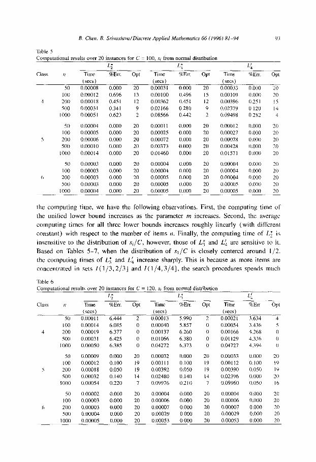
Table S
Computational results over 20 instances for C = 100, Si from normal distribution
L; LT G
Class II Time %ElT. Opt Time %Err. Opt Time %ElT. Opt
SO
(sea)
0.00008 0.000 20
(sea) 0.0003 1 0.000 20
(sets)
0.00033 0.000 20
100 0.696 0.00100 I5 0.000
4 0.00018 I2 0.4.51 0.00396 I
500 I I 0.02166 9 0.120
IO00 0.0005 I 0.623 2 0.08566 0.442 2 0.09498 0.282 4
SO 0.00004 0.000 20 0.000 I I 0.000 20 0.000 I2 0.000 20
100 0.00005 0.000 20 0.00025 0.000 20 0.00027 0.000 20
s 200 0.00006 0.000 20 0.00072 0.000 20 0.00078 0.000 20
500 0.00010 0.000 20 0.00373 0.000 20 0.00428 0.000 20
IO00 0.00014 0.000 20 0.01460 0.000 20 0.01571 0.000 20
SO 0.00003 0.000 20 0.00004 0.000 20 0.00004 0.000 20
100 0.00003 0.000 20 0.00004 0.000 20 0.00004 0.000 20
6 200 0.00003 0.000 20 0.00005 0.000 20 0.00004 0.000 20
500 0.00003 0.000 20 0.00005 0.000 20 0.00005 0.000 20
IO00 0.00004 0.000 20 0.00005 0.000 20 0.00005 0.000 20
the computing time, we have the following observations. First, the computing time of
the unified lower bound increases as the parameter m increases. Second, the average
computing times for all three lower bounds increases roughly linearly (with different
constant) with respect to the number of items ~1. Finally, the computing time of 15; is
insensitive to the distribution of Si/C, however, those of L; and Li are sensitive to it.
Based on Tables 5-7, when the distribution of st/C is closely centered around l/2,
the computing times of L; and Li increase sharply. This is because as more items are
concentrated in sets I( l/3,2/3] and I ( l/4,3/4], the search procedures spends much
Table 6 Computational results over 20 instances for C = 120, .Yi from normal distribution
L; L; G
Class II Time %EIX Opt Time BEIT. Opt Time %Ell.. opt
(sets) (sea) (sets) SO 0.00011 6.444 2 0.00013 5.990 2 0.0002 I 3.634 4
100 0.00014 6.085 0 0.00040 5.857 0 0.00054 3.436 5
4 200 0.00019 6.377 0 0.00 I37 6.260 0 0.00166 4.268 0
500 0.0003 1 6.425 0 0.01066 6.380 0 0.01129 4.336 0
1000 0.00050 6.385 0 0.04272 6.373 0 0.04727 4.394 0
SO 0.00009 0.000 20 0.00032 0.000 20 0.00033 0.000 20
100 0.00012 0.100 19 0.001 I I 0.100 19 0.001 I2 0.100 19 5 200 0.00018 0.050 19 0.00392 0.050 I9 0.00390 0.050 I9
500 0.00032 0.140 14 0.02480 0.140 14 0.02396 0.000 20 IO00 0.00054 0.220 7 0.09976 0.210 7 0.09960 o.oso I6
SO 0.00002 0.000 20 0.00004 0.000 20 0.00004 0.000 20
100 0.00003 0.000 20 0.00006 0.000 20 0.00006 0.000 20
6 200 0.00003 0.000 20 0.00007 0.000 20 0.00007 0.000 20 500 0.00004 0.000 20 0.00029 0.000 20 0.00029 0.000 20
IO00 0.00005 0.000 20 0.00053 0.000 20 0.00053 0.000 20
94 B. Chen, B. Srivastava/Discrete Applied Mathematics 66 (1996) 81-94
Table 7 Computational results over 20 instances for C = 1.50, si from normal distribution
L; L3* L;
Class n Time %EX Opt Time BEIT. Opt Time %Err Opt
50
(sets) 0.00006 12.985 0
(sets) 0.00005 4.622 6
(sets) 0.00012 4.622 6
100 0.00010 11.885 0 0.00007 3.706 1 0.00020 3.706 1 4 200 0.00017 11.799 0 0.00011 4.211 0 0.00036 4.211 0
500 0.00039 11.901 0 0.00022 4.23 1 0 0.00096 4.23 1 0
1000 0.0006 1 11.892 0 0.00040 4.168 0 0.00190 4.168 0
50 0.00011 6.498 2 0.00006 6.498 2 0.00014 3.888 7
100 0.00016 5.793 0 0.00016 5.674 0 0.00042 3.051 3
5 200 0.00024 4.680 0 0.00020 4.680 0 0.00064 2.610 1 500 0.00034 5.084 0 0.00094 5.084 0 0.00182 3.315 0
1000 0.00055 4.982 0 0.00365 4.982 0 0.00534 3.212 0
50 0.00008 0.000 20 0.00030 0.000 20 0.00032 0.000 20
100 0.00011 0.000 20 0.00111 0.000 20 0.00111 0.000 20
6 200 0.00016 0.000 20 0.00397 0.000 20 0.00392 0.000 20
500 0.00032 0.000 20 0.02543 0.000 20 0.02524 0.000 20
1000 0.00053 0.000 20 0.10944 0.000 20 0.09763 0.000 20
more time in computing N( l/3,1 ] and LN( l/4,1 1, the key elements of Li and Li.
Acknowledgements
The authors wish to thank the referee for the careful review and many valuable
suggestions, in particular in simplifying the proof of Theorem 2.3 and for pointing out
an error in the proof of Theorem 3.2 on an earlier version of this paper.
References
111
121
131
141
I51
(61
E.G. Coffman Jr, M.R. Garey and D.S. Johnson, Approximation algorithms for bin-packing - An updated
survey, in: G. Ausiello, M. Lucertini and I? Serafini, eds., Algorithm Design for Computer System Design
(Springer, Vienna, 1984).
M.R. Garey and D.S. Johnson, Computers and Intractability: A Guide to the Theory of NP-Completeness
(Freeman, San Francisco, CA, 1979).
Y.-D. Kim and C.A. Yano, Heuristic approaches for loading problems in flexible manufacturing systems,
IIE Trans. 25 (1993) 26-39.
S. Martello and I? Toth, Lower bounds and reduction procedures for the bin packing problem, Discrete
Appl. Math. 28 (1990) 59-70.
S. Martello and I? Toth, Knapsack Problems: Algorithms and Computer Implementations, (Wiley, New
York, 1990).
H.L. Ong, M.J. Magazine and T.S. Wee, Probabilistic analysis of bin packing heuristics, Oper. Res. 32
( 1984) 983-998.


![Approximation schemes Bin packing problem. Bin Packing problem Given n items with sizes a 1,…,a n (0,1]. Find a packing in unit-sized bins that minimizes](https://img.pdfslide.net/doc/110x75/56649e7a5503460f94b7a5ef/approximation-schemes-bin-packing-problem-bin-packing-problem-given-n-items.jpg)