Embed Size (px)
Citation preview
An independent component analysis filtering approach
for estimating continental hydrology in the GRACE
gravity data
Frederic Frappart, Guillaume Ramillien, Marc Leblanc, Sarah Tweed,
Marie-Paule Bonnet, Philippe Maisongrande
To cite this version:
Frederic Frappart, Guillaume Ramillien, Marc Leblanc, Sarah Tweed, Marie-Paule Bonnet, etal.. An independent component analysis filtering approach for estimating continental hydrologyin the GRACE gravity data. Remote Sensing of Environment, Elsevier, 2011, 115 (1), pp.187-204. <10.1016/j.rse.2010.08.017>. <hal-00533212>
HAL Id: hal-00533212
https://hal.archives-ouvertes.fr/hal-00533212
Submitted on 5 Nov 2010
HAL is a multi-disciplinary open accessarchive for the deposit and dissemination of sci-entific research documents, whether they are pub-lished or not. The documents may come fromteaching and research institutions in France orabroad, or from public or private research centers.
L’archive ouverte pluridisciplinaire HAL, estdestinee au depot et a la diffusion de documentsscientifiques de niveau recherche, publies ou non,emanant des etablissements d’enseignement et derecherche francais ou etrangers, des laboratoirespublics ou prives.

1
An Independent Component Analysis filtering approach for 1
estimating continental hydrology in the GRACE gravity 2
data 3
4
Frédéric Frappart (1), Guillaume Ramillien (2), Marc Leblanc (3), Sarah O. Tweed (3), 5
Marie-Paule Bonnet (1), Philippe Maisongrande (4) 6 7
(1) Université de Toulouse, UPS, OMP, LMTG, 14 Avenue Edouard Belin, 31400 Toulouse, 8
France ([email protected], [email protected]) 9
10
(2) Université de Toulouse, UPS, OMP, DTP, 14 Avenue Edouard Belin, 31400 Toulouse, 11
France ([email protected]) 12
13
(3) Hydrological Sciences Research Unit, School of Earth and Environmental Sciences, James 14
Cook University, Cairns, Queensland, Australia ([email protected], 15
17
(4) Université de Toulouse, UPS, OMP, LEGOS, 14 Avenue Edouard Belin, 31400 Toulouse, 18
France ([email protected]) 19
20
21
22
23
24
25
26
27
28
Submitted to Remote Sensing of Environment in August 2010 29
30
*Manuscript
2
Abstract: 31 32
An approach based on Independent Component Analysis (ICA) has been applied on a 33
combination of monthly GRACE satellite solutions computed from official providers (CSR, 34
JPL and GFZ), to separate useful geophysical signals from important striping undulations. We 35
pre-filtered the raw GRACE Level-2 solutions using Gaussian filters of 300, 400, 500-km of 36
radius to verify the non-gaussianity condition which is necessary to apply the ICA. This linear 37
inverse approach ensures to separate components of the observed gravity field which are 38
statistically independent. The most energetic component found by ICA corresponds mainly to 39
the contribution of continental water mass change. Series of ICA-estimated global maps of 40
continental water storage have been produced over 08/2002-07/2009. Our ICA estimates were 41
compared with the solutions obtained using other post-processings of GRACE Level-2 data, 42
such as destriping and Gaussian filtering, at global and basin scales. Besides, they have been 43
validated with in situ measurements in the Murray Darling Basin. Our computed ICA grids 44
are consistent with the different approaches. Moreover, the ICA-derived time-series of water 45
masses showed less north-south spurious gravity signals and improved filtering of unrealistic 46
hydrological features at the basin-scale compared with solutions obtained using other filtering 47
methods. 48
49
3
1. Introduction 50
51
Continental water storage is a key component of global hydrological cycles and plays a major 52
climate system via controls over water, energy and biogeochemical fluxes. 53
In spite of its importance, the total continental water storage is not well-known at regional and 54
global scales because of the lack of in situ observations and systematic monitoring of the 55
groundwaters (Alsdorf and Lettenmaier, 2003). 56
The Gravity Recovery and Climate Experiment (GRACE) mission provides a global mapping 57
of the time-variations of the gravity field at an unprecedented resolution of ~400 km and a 58
precision of ~1 cm in terms of geoid height. Tiny variations of gravity are mainly due to 59
redistribution of mass inside the fluid envelops of the Earth (i.e., atmosphere, oceans and 60
continental water storage) from monthly to decade timescales (Tapley et al., 2004). 61
Pre-processing of GRACE data is made by several providers (University of Texas, Centre for 62
Space Researh - CSR, Jet Propulsion Laboratory - JPL, GeoForschungsZentrum - GFZ and 63
Groupe de Recherche en Géodésie Spatiale - GRGS) which produce residual GRACE 64
spherical harmonic solutions that mainly represent continental hydrology as they are corrected 65
from known mass transfers using ad hoc oceanic models (i.e., Toulouse Unstructured Grid 66
Ocean model 2D - T-UGOm 2D) and atmospheric reanalyses from National Centers for 67
Environmental Prediction (NCEP) and European Centre for Medium Weather Forecasting 68
(ECMWF). Unfortunately these solutions suffer from the presence of important north-south 69
striping due to orbit resonance in spherical harmonics determination and aliasing of short-time 70
phenomena which are geophysically unrealistic. 71
Since its launch in March 2002, the GRACE terrestrial water storage anomalies have been 72
increasingly used for large-scale hydrological applications (see Ramillien et al., 2008; Schmitt 73
et al., 2008 for reviews). They demonstrated a great potential to monitor extreme hydrological 74
events (Andersen et al., 2005; Seitz et al., 2008; Chen et al., 2009), to estimate water storage 75
variations in the soil (Frappart et al., 2008), the aquifers (Rodell et al., 2007; Strassberg et al., 76
2007; Leblanc et al., 2009) and the snowpack (Frappart et al., 2006; in press), and 77
hydrological fluxes, such as basin-scale evapotranspiration (Rodell et al., 2004a; Ramillien et 78
al. , 2006a) and discharge (Syed et al. , 2009). 79
Because of this problem of striping that limits geophysical interpretation, different post-80
processing approaches for filtering GRACE geoid solutions have been proposed to extract 81
useful geophysical signals (see Ramillien et al., 2008; Schmidt et al., 2008 for reviews). 82
These include the classical isotropic Gaussian filter (Jekeli, 1981), various optimal filtering 83
4
decorrelation of GRACE errors (Han et al., 2005; Seo and Wilson, 2005; Swenson and Wahr, 84
2006; Sasgen et al., 2006; Kusche, 2007; Klees et al., 2008), as well as statistical constraints 85
on the time evolution of GRACE coefficients (Davis et al., 2008) or from global hydrology 86
models (Ramillien et al., 2005). However, these filtering techniques remain imperfect as they 87
require input non-objective a priori information which are most of the time simply tuned by 88
hand (e.g. choosing the cutting wavelength while using the Gaussian filtering) or based on 89
other rules-of-thumb. 90
We propose another post-processing approach of the Level-2 GRACE solutions by 91
considering completely objective constraints, so that the gravity component of the observed 92
signals is forced to be uncorrelated numerically using an Independent Component Analysis 93
(ICA) technique. This approach does not require a priori information except the assumption 94
of statistical independence of the elementary signals that compose the observations, i.e., 95
geophysical and spurious noise. The efficiency of ICA to separate gravity signals and noise 96
from combined GRACE solutions has previously been demonstrated on one month of Level-2 97
solutions (Frappart et al., 2010). In this paper, we use this new statistical linear method to 98
derive complete time series of continental water mass change. 99
The first part of this article presents the datasets used in this study: the monthly GRACE 100
solutions to be inverted by ICA and to be used for comparisons, and the in situ data used for 101
validation of our estimates over the Murray Darling drainage basin (~ 1 million of km²). This 102
region has been selected for validation because of available dense hydrological observations. 103
The second part outlines the three steps of the ICA methodology. Then the third and fourth 104
parts present results and comparisons with other post-processed GRACE solutions at global 105
and regional scales, and in situ measurements for the Murray Darling Basin respectively. 106
Error balance of the ICA-based solutions is also made by considering the effect of spectrum 107
truncation, leakage and formal uncertainties. 108
109
2. Datasets 110 111
2.1. The GRACE data 112
113
The GRACE mission, sponsored by National Aeronautics and Space Administration (NASA) 114
and Deutsches Zentrum für Luft- und Raumfahrt (DLR), has been collecting data since mid-115
2002. Monthly gravity models are determined from the analysis of GRACE orbit 116
perturbations in terms of Stokes spherical harmonic coefficients, i.e., geopotential or geoid 117
heights. The geoid is an equipotential surface of the gravity field that coincide with mean sea 118
5
level. For the very first time, monthly global maps of the gravity time-variations can be 119
derived from GRACE measurements, and hence, to estimate the distribution of the change of 120
mass in the Earth system. 121
122
2.1.1. The Level-2 raw solutions 123
124
The Level-2 raw data consist of monthly estimates of geo-potential coefficients adjusted for 125
each 30-day period from raw along-track GRACE measurements by different research groups 126
(i.e., CSR, GFZ and JPL). These coefficients are developed up to a degree 60 (or spatial 127
resolution of 333 km) and corrected for oceanic and atmospheric effects (Bettadpur, 2007) to 128
obtain residual global grids of ocean and land signals corrupted by a strong noise. These data 129
are available at: ftp://podaac.jpl.nasa.gov/grace/. 130
131
2.1.2. The destriped and smoothed solutions 132
133
The monthly raw solutions (RL04) from CSR, GFZ, and JPL were destriped and smoothed by 134
Chambers (2006) for hydrological purposes. These three datasets are available for several 135
averaging radii (0, 300 and 500 km on the continents and 300, 500 and 750 km on the oceans) 136
at ftp://podaac.jpl.nasa.gov/tellus/grace/monthly. 137
138
In this study, we used the Level-2 RL04 raw data from CSR, GFZ and JPL, that we filtered 139
with a Gaussian filter for radii of 300, 400 and 500 km, and the destriped and smoothed 140
solutions for the averaging radii of 300 and 500 km over land. 141
142
2.2. The hydrological data for the Murray Darling Basin 143
144
In the predominantly semiarid Murray Darling Basin, most of the surface water is regulated 145
using a network of reservoirs, lakes and weirs (Kirby et al., 2006) and the surface water stored 146
in these systems represent most of the total surface water (SW) present across the basin. A 147
daily time series of the total surface water storage in the network of reservoirs, lakes, weirs 148
and in-channel storage was obtained from the Murray-Darling Basin Commission and the 149
state governments from January 2000 to December 2008. 150
In the Murray Darling Basin, we derived monthly soil moisture (SM) storage values for the 151
basin from January 2000 to December 2008 from the NOAH land surface model (Ek et al., 152
6
2003), with the NOAH simulations being driven (parameterization and forcing) by the Global 153
Land Data Assimilation System (Rodell et al., 2004b). The NOAH model simulates surface 154
energy and water fluxes/budgets (including soil moisture) in response to near-surface 155
atmospheric forcing and depending on surface conditions (e.g., vegetation state, soil texture 156
and slope) (Ek et al., 2003). The NOAH model outputs of soil moisture estimates have a 1° 157
spatial resolution and, using four soil layers, are representative of the top 2 m of the soil. 158
In situ estimates of annual changes in the total groundwater storage (GW) across the drainage 159
basin were obtained from an analysis of groundwater levels observed in government 160
monitoring bores from 2000 to 2008. Compared to earlier estimates by Leblanc et al. (2009), 161
the groundwater estimates presented in this paper provide an update of the in situ water level 162
and a refinement of the distribution of the aquifers storage capacity. 163
Assuming that (1) the shallow aquifers across the Murray-Darling drainage basin are 164
hydraulically connected and that (2) at a large scale the fractured aquifers can be assimilated 165
to a porous media, changes in groundwater storage across the area can be estimated from 166
observations of groundwater levels (e.g., Rodell et al., 2007; Strassberg et al., 2007). 167
Variations in groundwater storage ( GW) were estimated from in situ measurements as: 168
GW yS S H (1) 169
where Sy is the aquifer specific yield (%) and H is the groundwater level (L-1
) observed in 170
monitoring bores. Groundwater level data (H) were sourced from State Government 171
departments that are part of the Murray-Darling Basin (QLD; Natural Resources and Mines; 172
NSW; Department of Water and Energy; VIC; Department of Sustainability and 173
Environment; and SA; Department of Water Land and Biodiversity Conservation). Only 174
government observation bores (production bores excluded) with an average saturated zone 175
<50 m from the bottom of the screened interval were selected. Deeper bores were excluded as 176
they can reflect processes occurring on longer time scales (Fetter, 2001). A total of 6183 177
representative bores for the unconfined aquifers across the Murray Darling Basin were 178
selected on the basis of construction and monitoring details obtained from the State 179
departments. ~85% (5075) of the selected monitoring bores have a maximum annual standard 180
deviation of the groundwater levels below 2 m for the study period (2000-2008) and were 181
used to analyze the annual changes in groundwater storage during the period 2000 to 2008. 182
The remaining 15% of the observation bores, with the highest annual standard deviation, were 183
discarded as possibly under the immediate influence of local pumping or irrigation. The 184
potential influence of irrigation on some of the groundwater data is limited because during 185
7
this period of drought, irrigation is substantially reduced across the basin. Changes in 186
groundwater levels across the basin were estimated using an annual time step as most 187
monitoring bores have limited groundwater level measurements in any year (50% of bores 188
with 5 measures per year). The annual median of the groundwater level was first calculated 189
for each bore and change at a bore was computed as the difference of annual median 190
groundwater level between two consecutive years. For each year, a spatial interpolation of the 191
groundwater level change was performed across the basin using a kriging technique. Spatial 192
averages of annual groundwater level change were computed for each aquifer group. 193
The Murray Darling drainage basin comprises several unconfined aquifers that can be 194
regrouped into 3 categories according to their lithology: a clayey sand aquifer group 195
(including the aquifers Narrabri (part of), Cowra, Shepparton, and Murrumbidgee (part of)); a 196
sandy clay aquifer group (including the aquifers Narrabri (part of), Parilla, Far west, and 197
Calivil (part of)); and a fractured rock aquifer group comprising metasediments, volcanics and 198
weathered granite (including the aquifers Murrumbidgee (part of), North central, North east, 199
Central west, Barwon, and Queensland boundary). The specific yield is estimated to range 200
from 5 to 10% for the clayey sand unconfined aquifer group (Macumber, 1999; Cresswell et 201
al., 2003; Hekmeijer and Dawes, 2003a; CSIRO, 2008); from 10 to 15% for the shallow 202
sandy clay unconfined aquifer group (Macumber, 1999; Urbano et al., 2004); and from 1 to 203
10% for the fractured rock aquifer group (Cresswell et al., 2003; Hekmeijer and Dawes, 204
2003b; Smitt et al., 2003; Petheram et al., 2003). In situ estimates of changes in GW storage 205
are calculated using the spatially averaged change in annual groundwater level across each 206
type of unconfined aquifer group and the mean value of the specific yield for that group using 207
(Eq. 1); while the range of possible values for the specific yield was used to estimate the 208
uncertainty. 209
Groundwater changes in the deep, confined aquifers (mostly GAB and Renmark aquifers) are 210
either due to: 1) a change in groundwater recharge at the unconfined outcrop; 2) shallow 211
pumping at the unconfined outcrop or 3) deep pumping in confined areas for farming 212
(irrigation and cattle industry). GRACE TWS estimates accounts for all possible sources of 213
influence, while GW in situ estimates only include those occurring across the outcrop. Total 214
pumping from the deep, confined aquifers was estimated to amount to -0.42 km3 .yr
-1 in 2000 215
(Ife and Skelt, 2004), while groundwater pumping across the basin was -1.6 km3 in 2002216
2003 (Kirby et al., 2006). To allow direct comparison between TWS and in-situ GW 217
estimates, pumping from the deep aquifers was added to the in-situ GW time series assuming 218
the -0.42 km3 .yr
-1 pumping rate remained constant during the study period. 219
8
220
3. Methodology 221
222 3.1. ICA-based filter 223
224
ICA is a powerful method for separating a multivariate signal into subcomponents assuming 225
their mutual statistical independence (Comon, 1994; De Lathauwer et al., 2000). It is 226
commonly used for blind signals separation and has various practical applications (Hyvärinen 227
and Oja, 2000), including telecommunications (Ritsaniemi and Joutsensalo, 1999; Cristescu et 228
al., 2000), medical signal processing (Vigário, 1997; van Hateren and van der Schaaf, 1998), 229
speech signal processing (Stone, 2004), and electrical engineering (Gelle et al., 2001; 230
Pöyhönen et al., 2003). 231
Assuming that an observation vector y collected from N sensors is the combination of P (N 232
P) independent sources represented by the source vector x, the following linear statistical 233
model can be considered: 234
y Mx (2) 235
where M is the mixing matrix whose elements mij (1 i N, 1 j P) indicate to what extent 236
the jth
source contribute to the ith
observation. The columns {mj} are the mixing vectors. 237
The goal of ICA is to estimate the mixing matrix M and/or the corresponding realizations of 238
the source vector x, only knowing the realizations of the observation vector y, under the 239
assumptions (De Lathauwer et al., 2000): 240
1) the mixing vectors are linearly independent, 241
2) the sources are statistically independent. 242
The original sources x can be simply recovered by multiplying the observed signals y with the 243
inverse of the mixing matrix 244
1x M y (3) 245
To retrieve the original source signals, at least N observations are necessary if N sources are 246
present. ICA remains applicable for square or over-determined problems. ICA proceeds by 247
maximizing the statistical independence of the estimated components. As a condition of 248
applicability of the method, non-Gaussianity of the input signals has to be checked. The 249
central limit theorem is then used for measuring the statistical independence of the 250
components. Classical algorithms for ICA use centering and whitening based on eigenvalue 251
decomposition (EVD) and reduction of dimension as main processing steps. Whitening 252
ensures that the input observations are equally treated before dimension reduction. 253
9
ICA consists of three numerical steps. The first step of ICA is to centre the observed vector, 254
i.e., to substract the mean vector m E y to make y a zero mean variable. The second step 255
consists in whitening the vector y to remove any correlation between the components of the 256
observed vector. In other words, the components of the white vector ~y have to be 257
uncorrelated and their variances equal to unity. Letting tC E yy be the correlation matrix 258
of the input data, we define a linear transform B that verifies the two following conditions: 259
y By (4) 260
and: 261
t
PE yy I (5) 262
where IP is identity matrix of dimension P x P. 263
This is easily accomplished by considering: 264
1
2B C (6) 265
The whitening is obtained using an EVD of the covariance matrix C: 266
tC EDE (7) 267
where E is the orthogonal matrix of the eigenvectors of C and D is the diagonal matrix of its 268
eigenvalues. D=diag(d1 dP) as a reduction of the dimension of the data to the number of 269
independent components (IC) P is performed, discarding the too small eigenvalues. 270
For the third step, an orthogonal transformation of the whitened signals is used to find the 271
separated sources by rotation of the joint density. The appropriate rotation is obtained by 272
maximizing the non-normality of the marginal densities, since a linear mixture of independent 273
random variables is necessarily more Gaussian than the original components. 274
Many algorithms of different complexities have been developed for ICA (Stone, 2004). The 275
FastICA algorithm, a computationally highly efficient method for performing the estimation 276
of ICA (Hyvärinen and Oja, 2000) has been considered to separate satellite gravity signals. It 277
uses a fixed-point iteration scheme that has been found to be 10 to 100 times faster than 278
conventional gradient methods for ICA (Hyvärinen, 1999). 279
We used the FastICA algorithm (available at http://www.cis.hut.fi/projects/ica/fastica/) to 280
unravel the IC of the monthly gravity field anomaly in the Level-2 GRACE products. We 281
previously demonstrated, on a synthetic case, that land and ocean mass anomalies are 282
statistically independent from the north-south stripes using information from land and ocean 283
models and simulated noise (Frappart et al., 2010). Considering that the GRACE Level-2 284
products from CSR, GFZ and JPL are different observations of the same monthly gravity 285
10
anomaly and, that the land hydrology and the north-south stripes are the independent sources, 286
we applied this methodology to the complete 2002-2009 time series. The raw Level-2 287
GRACE solutions present Gaussian histograms which prevent the successful application of 288
the ICA method. To ensure the non-Gaussianity of the observations, the raw data have been 289
preprocessed using Gaussian filters with averaging radii of 300, 400 and 500 km as in 290
Frappart et al. (2010). 291
292
3.2. Time-series of basin-scale total water storage average 293
294
For a given month t, the regional average of land water volume V(t) (or height h(t)) over a 295
given river basin of area A is simply computed from the water height hj, with 296
(expressed in terms of mm of equivalent-water height) inside A, and the elementary surface 297
Re2
sin j : 298
2( ) ( , , )sin je j j j
j A
V t R h t (8) 299
2
( ) ( , , )sinejj j j
j A
Rh t h t
A (9) 300
where j and j are co-latitude and longitude of the jth
point, and are the grid steps in 301
longitude and latitude respectively (generally = ). In practice, all points of A used in (Eq. 302
8 and 9) are extracted for the eleven drainage basins masks at a 0.5° resolution provided by 303
Oki and Sud (1998), except for the Murray Darling Basin where we used basin limits from 304
Leblanc et al. (2009). 305
306
3.3. Regional estimates of formal error 307
308
As ICA provides separated solutions which have Gaussian distributions, the variance of the 309
regional average for a given basin is: 310
2
2 1
2
L
k
kformal
L (10) 311
where formal is the regional formal error, k is the formal error at a grid point number k, and L 312
is the number of points used in the regional averaging. 313
If the points inside the considered basin are independent, this relation is slightly simplified: 314
kformal
L (11) 315
316
11
3.4. Frequency cut-off error estimates 317
318
Error in frequency cut-off represents the loss of energy in the short spatial wavelength due to 319
the low-pass harmonic decomposition of the signals that is stopped at the maximum degree 320
N1. For the GRACE solution separated by ICA; N1=60, thus the spatial resolution is limited 321
and stopped at ~330 km by construction. This error is simply evaluated by considering the 322
difference of reconstructing the remaining spectrum between two cutting harmonic degrees N1 323
and N2, where N2 > N1 and N2 should be large enough compared to N1 (e.g., N2=300 in study): 324
2 1 2
10 0
N N N
truncation n n n
n n n N
(12) 325
using the scalar product 0
n
n nm nm nm nm
m
C A S B (13) 326
where Anm and Bnm are the harmonic coefficients of the considered geographical mask, and 327
Cnm and Snm are the harmonic coefficients of the water masses. 328
329
3.5. Leakage error estimates 330
331
We define « leakage » as the portion of signals from outside the considered geographical 332
region that pollutes the estimates. By construction, this effect can be seen as the 333
limitation of the geoid signals degree in the spherical harmonics representation. For each 334
basin and at each period of time, leakage is simply computed as the average of outside values 335
by using an « inverse » mask, which is 0 and 1 in and out of the region respectively, 336
developed in spherical harmonics and then truncated at degree 60. This method of 337
computing leakage of continental water mass has been previously proposed for 338
the entire continent of Antarctica (Ramillien et al., 2006b), which revealed 339
that the seasonal amplitude of this type of error can be quite important (e.g. up to 10% of the 340
geophysical signals). In case of no leakage, this average should be zero (at least, it decreases 341
with the maximum degree of decomposition). However, the maximum leakage of continental 342
hydrology remains in the order of the signals magnitude itself. 343
344
4. Results and discussion 345 346
4.1. ICA-filtered land water solutions 347
348
The methodology presented in Frappart et al. (2010) has been applied to the Level-2 RL04 349
raw monthly GRACE solutions from CSR, GFZ and JPL, preprocessed using a Gaussian filter 350
with a radius of 300, 400 and 500 km, over the period July 2002 to July 2009. The results of 351
this filtering method is presented in Fig. 1 for four different time periods (March and 352
12
September 2006, March 2007 and March 2008) using the GFZ solutions Gaussian-filtered 353
with a radius of 400 km. Only the ICA-based GFZ solution is presented since, for a specific 354
radius, the ICA-based CSR, GFZ, and JPL solutions only differ from a scaling factor for each 355
specific component. The ICA-filtered CSR, GFZ, and JPL solutions are obtained by 356
multiplying the jth
IC with the jth
mixing vector (2). As the last two modes correspond to the 357
north south stripes, we present their sum in Fig. 1. 358
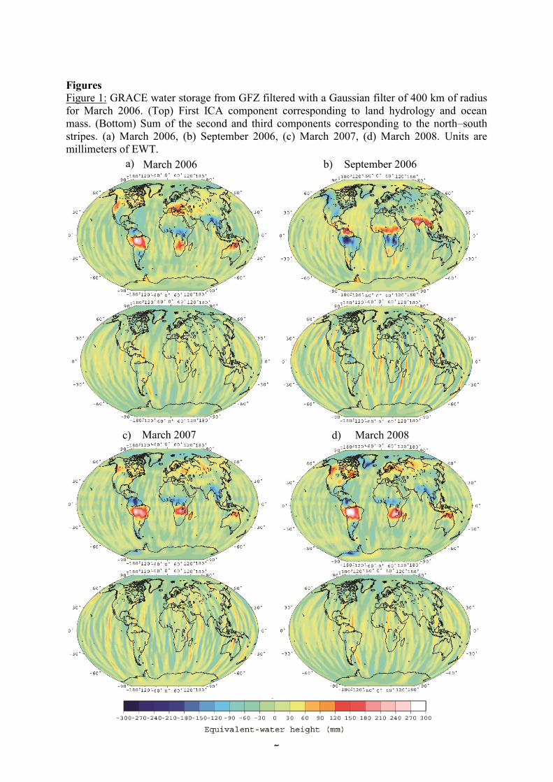
The first component is clearly ascribed to terrestrial water storage with variations in the range 359
of 450 mm of Equivalent Water Thickness (EWT) for an averaging radius of 400 km. The 360
larger water mass anomalies are observed in the tropical regions, i.e., the Amazon, the Congo, 361
the Ganges and the Mekong Basins, and at high latitudes in the northern hemisphere. The 362
components 2 and 3 correspond to the north-south stripes due to 363
orbits. They are smaller than the first component by a factor of 3 or 4 as previously found 364
(Frappart et al., 2010). 365
The FastICA algorithm was unable to retrieve realistic patterns and/or amplitudes of TWS-366
derived from GRACE data preprocessed using a Gaussian filter with a radius 300 km for 367
several months (02/2003, 06 to 11/2004, 02/2005, 07/2005, 01/2006, 01/2007, 02/2009). 368
Some of these dates, such as the period between June and November 2004, correspond to 369
deep resonance between the satellites caused by an almost exact repeat of the orbit, 370
responsible for a significantly poorer accuracy of the monthly solutions (Chambers, 2006). As 371
ICA is based on the assumption of independence of the sources, if the sources exhibit similar 372
statistical distribution, the algorithm is unable to separate them. 373
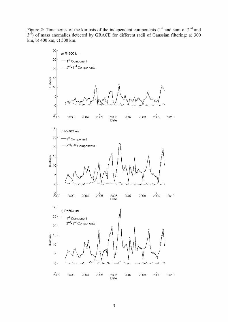
A classical measure of the peakiness of the probability distribution is given by the kurtosis. 374
The kurtosis Ky is dimensionless fourth moment of a variable y and classically defined as: 375
4
22
y
E yK
E y (14) 376
If the probability density function of y is purely Gaussian, its kurtosis has the numerical value 377
of 3. In the followings, we will consider the excess of kurtosis (Ky-3) and refer to the kurtosis 378
as it is commonly done. So a variable y will be Gaussian if its kurtosis remains close to 0. 379
The time series of the kurtosis of the sources separated using ICA are presented in Fig. 2 for 380
different radii of Gaussian filtering (300, 400 and 500 km) of GRACE mass anomalies. The 381
kurtosis of the sum of the 2nd
and 3rd
ICs, corresponding to the north-south stripes, is most of 382
the time, close to 0; that is to say that the meridian oriented spurious signals is almost 383
Gaussian. Almost equal values of the kurtosis for the 1st IC and the sum of the 2
nd and 3
rd ICs 384
13
can be observed for several months. Most of the time, they correspond to time steps where the 385
algorithm is unable to retrieve realistic TWS (02/2003, 08/2004, 11/2004, 02/2005, 01/2006, 386
01/2007, 02/2009). 387
We also observed that the number of time steps with only one IC (the outputs are identical to 388
the inputs, i.e., no independent sources are identified and hence no filtering was performed) 389
increases with the radius of the Gaussian filter (none at 300 km, 2 at 400 km, 7 at 500 km). 390
In the following, as the ICA-derived TWS with a Gaussian prefiltering of 300 km, exhibits an 391
important gap of 6 months in 2004, we will only consider the solutions obtained after a 392
preprocessing with a Gaussian filter for radii of 400 and 500 km (ICA400 and ICA500). 393
394
4.2. Global scale comparisons 395
396
Global scale comparisons have been achieved with commonly-used GRACE hydrology 397
preprocessings: the Gaussian filter (Jekeli, 1981) and the destriping method (Swenson and 398
Wahr, 2006) for several smoothing radii. 399
400
4.2.1. ICA versus Gaussian-filtered solutions 401
402
Advantages of extracting continental hydrology using ICA after a simple Gaussian filtering 403
have to be demonstrated for the complete period of availability of the GRACE Level-2 404
dataset, as it was for one period of GRACE Level-2 data in Frappart et al., (2010). Numerical 405
tests of comparisons before and after ICA have been made to show full utility of considering a 406
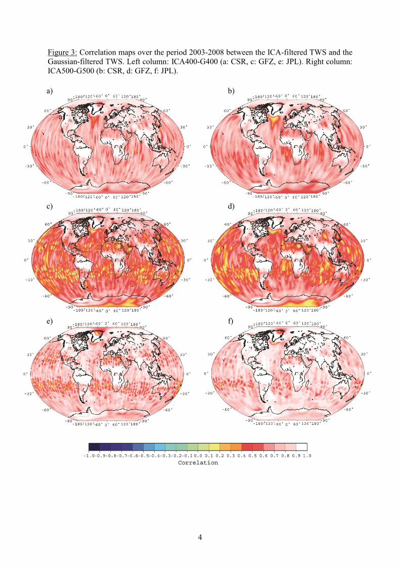
post-treatment by ICA for signals separation. For the period 2003-2008, we present 407
correlation (Fig. 3) and RMS (Fig. 4) maps computed between the ICA400 (respectively 408
ICA500) and Gaussian-filtered solutions with a radius of 400 km (500 km), named in the 409
followings G400 (G500). High correlation coefficients are generally observed over land 410
(greater than 0.9), increasing with the smoothing radius, especially over areas with large 411
hydrological signals, i.e., Amazon, Congo and Ganges basins, boreal regions. On the contrary, 412
low correlation values, structured as stripes, are located over arid and semi-arid regions 413
(southwest of the US, Sahara, Saudi Arabia, Gobi desert, centre of Australia), especially for 414
GFZ and JPL solutions. These important RMS differences between Gaussian and ICA-based 415
solutions reveal that the GRACE signals still contains remaining stripes after the Gaussian 416
filtering. This justifies that extracting the useful continental hydrology signals requires a 417
further processing. For this purpose, ICA succeeds in isolating this noise in its second and 418
third components (as illustrated in Figure 1). 419
14
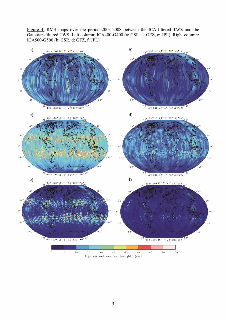
In Fig. 4, we observe that the spatial distribution of the RMS between ICA solutions and 420
Gaussian solutions presents north-south stripes with values generally lower than 30 mm, 421
except for some spots between (20 30)° of latitudes on the GFZ (Fig. 4c and d) and JPL 422
(Fig. 4e and e) solutions. The ICA approach allows the filtering of remnant stripes present in 423
the Gaussian solutions, especially for GFZ and JPL (Fig. 4c to f). These unrealistic structures 424
(stripes and spots), which correspond to resonances in the orbit of the satellites, are clearly 425
filtered out using the ICA approach (compare with Fig. 1). A more important smoothing due 426
to a larger radius caused a decrease of the RMS between ICA and Gaussian solutions (Fig 4a, 427
c and e). The RMS can reach 100 mm between ICA400 and G400 and only 65 mm between 428
ICA500 and G500 for the GFZ solutions. 429
430
4.2.2. ICA versus destriped and smoothed solutions 431
432
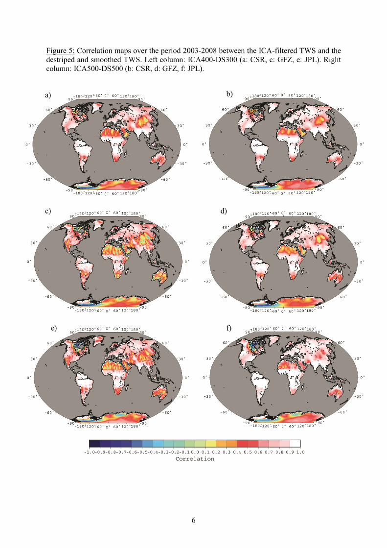
Similar to Fig. 3 and 4, we present correlation (Fig. 5) and RMS (Fig. 6) maps over the period 433
2003-2008; between ICA400 (ICA500 respectively) and destriped and smoothed solutions 434
with radii of 300 km (DS300) and 500 km (DS500), made available by Chambers (2006). The 435
correlation maps between ICA400 (respectively ICA500) and DS300 (DS500) exhibit very 436
similar patterns compared with those presented in Fig. 3, except in the McKenzie Basin and 437
Nunavut (northern Canada) where low correlation or negative correlations for GFZ and JPL 438
solutions (Fig. 5c to f) are found. 439
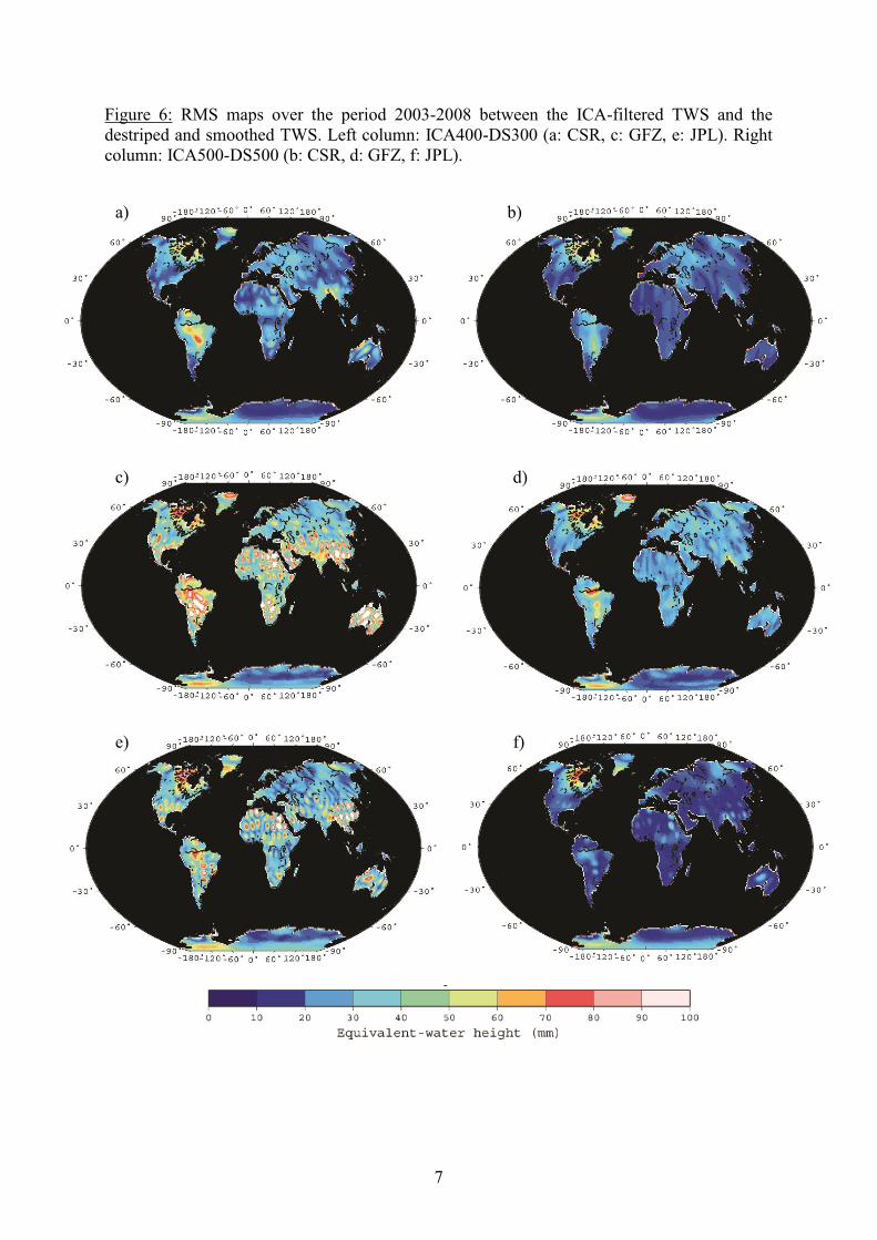
The RMS differences between ICA and destriped and smoothed solutions present low values 440
above 30° (or below -30°) of latitude (< 30 mm of EWT), with the exceptions of Nunavut in 441
northern Canada and extreme values (up to 100 mm) in the tropics. This is clearly due to the 442
low performance of the destriping method in areas close to Equator as previously mentioned 443
by Swenson and Wahr (2006) and Klees et al. (2008). These extrema are especially present in 444
the DS300 GFZ and JPL solutions. Some secondary maxima (up to 80 mm) are also noticed 445
for the GFZ and the JPL solutions. These important differences correspond to north-south 446
stripes that still appear in the destriped and smoothed solutions despite the filtering process 447
(and that can be filtered out by applying an ICA approach see the results for DS300 GFZ 448
solution of March 2006 in Fig. 7). For an averaging radius of 500 km, the RMS between 449
ICA500 and DS500 is lower than 20 to 30 mm, except for the Nunavut (Fig. 6b, d, f), along 450
the Parana stream (40 to 50 mm in the CSR solutions Fig. 6b), and along the Amazon and 451
Parana streams (60 to 80 mm in the GFZ solutions Fig. 6d). 452
15
These low spatial correlations suggest Gaussian-ICA provides at the least equivalent results 453
on the continents to the smoothing-destriping method. Besides, it is interesting that both 454
approaches are based on a pre-Gaussian filtering. Short wavelength differences between the 455
maps obtained separetely using ICA and destriping reveals the limitation of the destriping 456
which generates artefacts in the tropics. 457
458
4.2.3. Trend comparisons 459
460
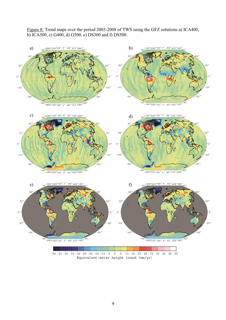
The effects of the stripes on the trends estimated using GRACE-based TWS is supposed to be 461
significant. From the time-series of TWS anomaly grids derived from GRACE (using 462
equation 1), the temporal trend, seasonal and semi-annual amplitudes were simultaneously 463
fitted by least-square adjustment at each grid point over the period 2003-2008 (see Frappart et 464
al., in press, for details). We present in Fig. 8 trends of TWS for ICA400 (Fig. 8a) and 465
ICA500 (Fig. 8b), for G400 (Fig. 8c) and G500 (Fig. 8d), and for DS300 (Fig. 8e) and DS500 466
(Fig. 8f). 467
The trend estimates exhibit large differences in spatial patterns and the amplitude of the 468
signal, especially between ICA and other processing methods. The most significant 469
differences over land (except Antarctica) are located at high latitudes, over Scandinavia, and 470
the Laurentide region, in the northeast of Canada. The ICA400 and ICA500 solutions present 471
negative trends of TWS (Fig. 8a and b), whereas the G400 and G500 and the DS300 and 472
DS500 present large positive trends (Fig. 8c to f). These two zones are strongly affected by 473
the post-glacial rebound (PGR) which has a specific signature in the observed gravity field. 474
This effect accounts for positive trends in these regions. According to the PGR models 475
developed by Peltier (2004) and Paulson et al. (2007), its intensity can be greater in these 476
regions than the trends measured by GRACE. For example, in the Nelson Basin, Frappart et 477
al. (in press) found a trend of TWS from GRACE of (4.5 0.2) mm/yr over 2003-2006, while 478
model-based estimates of PGR represents 18.8 mm/yr in this region. As the space and time 479
characteristics of the glacial isostatic adjustement (GIA) is different than the one from 480
continental hydrology, the ICA approach may have separated it from the signals only related 481
to the redistribution of water masses. Unfortunately, trends computed on the 2nd
and 3rd
ICs, 482
and their sum does not exclusively correspond to GIA, but to a mixture of geophysical 483
remaining signals and noise. It is also worth noticing that the gravity signature of the Sumatra 484
event in December 2004, which is clearly apparent on the Gaussian-filtered solutions (Fig. 8c 485
and d), is not visible in the 1st mode of the ICA solutions (Fig. 8a and b), but is present in the 486

16
sum of the 2nd
and 3rd
ICs. This confirms that the ICA is able to isolate a pure hydrological 487
mode in the GRACE products. 488
A second important difference between ICA solutions and Gaussian-filtered and destriped and 489
smoothed solutions concerns the impact of the filtering radius on the trends estimate. An 490
increase of the filtering radius causes a smoothing of the solutions, and, consequently, a 491
decrease of the intensity of the trends on Gaussian-filtered and destriped and smoothed 492
solutions (Fig. 8c to f). On the contrary, the intensity of the trends increases with radius of 493
prefiltering on the ICA solutions. The location of the extrema is also shifted. This change in 494
the location is a side-effect of the prefiltering with the Gaussian filter. A better location of the 495
trends is observed when a Gaussian-filter of 400 km of radius is used instead of 500 km (see 496
for instance the trends pattern in the Amazon and Orinoco Basins in Fig. 8a and b). 497
498
4.3. Basin scale comparisons 499
500
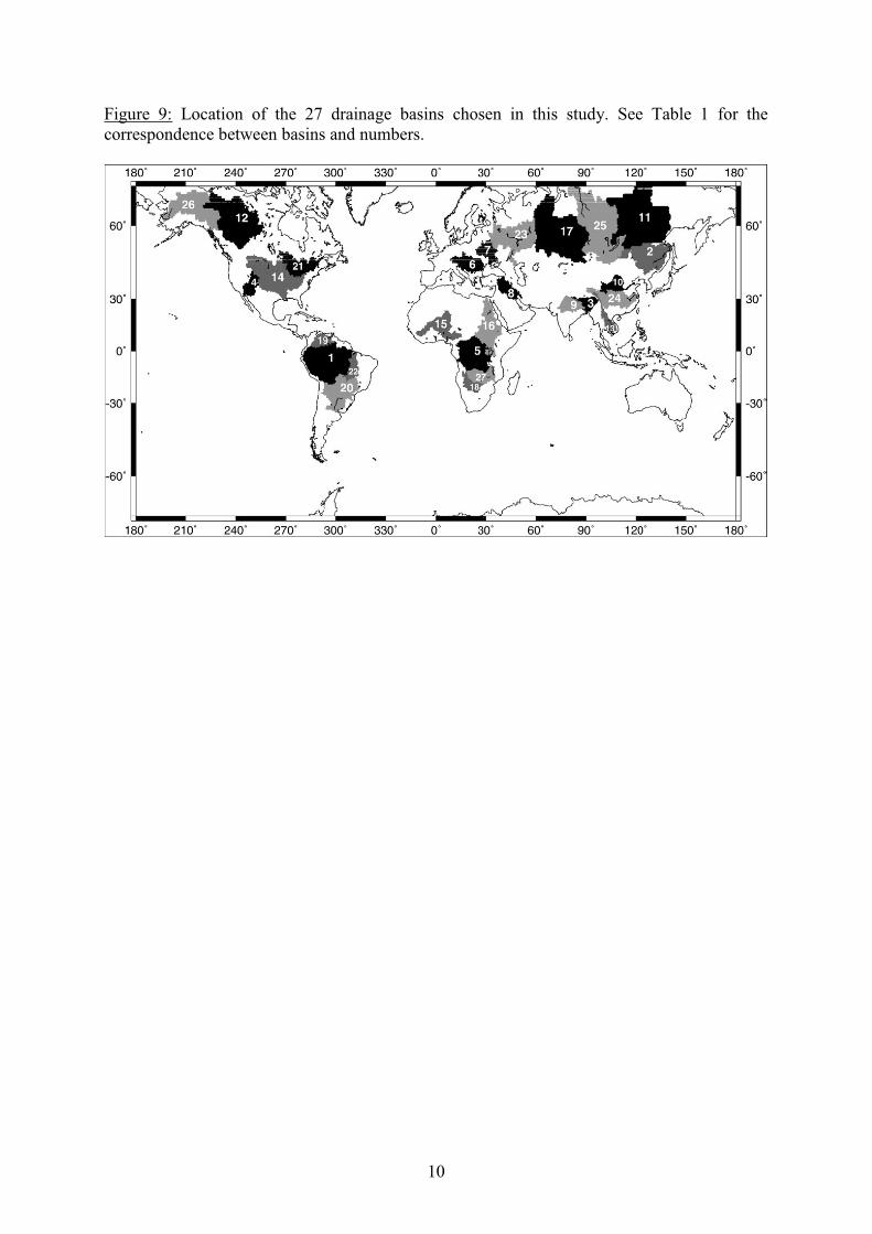
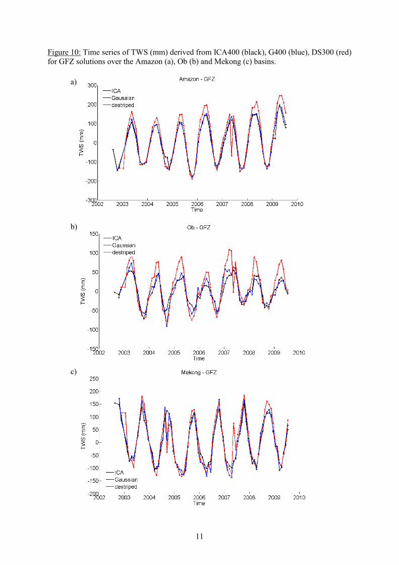
Changes in total water volume were estimated for 27 drainage basins whose locations are 501
shown in Fig. 9 (the corresponding areas are given in Table 1). ICA400 and ICA500 were 502
used to compute regional TWS averages versus time (Eq. 8 and 9). These times-series were 503
compared to the G400 and G500, and the DS300 and DS500 respectively. Examples of the 504
Amazon, the Ob and the Mekong basins for ICA400, G400 and DS300 (GFZ solutions) are 505
presented in Fig. 10. TWS exhibit very similar temporal patterns for all the types of filtering 506
radii and basins. The correlation coefficients between the ICA and the Gaussian-filtered, or 507
the ICA and the destriped and smoothed time series of TWS are greater than 0.9 for 21 out of 508
27 basins. For five other basins (Amur, Colorado, Hwang Ho, Parana, St Lawrence), most of 509
the correlation coefficients are greater than 0.8 or 0.9, and the others (generally the correlation 510
coefficients between ICA and destriped and smoothed GFZ solutions) greater than 0.65 or 511
0.7. The only exception is the McKenzie Basin where all the correlation coefficients between 512
ICA and destriped and smoothed are lower than 0.75 (r(ICA400,DS300) JPL=0.45 and r(ICA500,DS500) 513
JPL=0.51). For the GFZ solutions, some unrealistic peaks are present in the destriped and 514
smoothed TWS time series for some periods (Fig. 10a, 10b and 10c). These peaks only appear 515
on the Gaussian-filtered solutions for the smallest basins, such as the one of the Mekong river 516
(Fig. 10c), but are not present in the ICA-filtered solutions. RMS difference between ICA-517
filtered solutions and the other type of solutions are generally lower than 30 mm of equivalent 518
water height and logically decrease with the radius of filtering. Differences with ICA 519
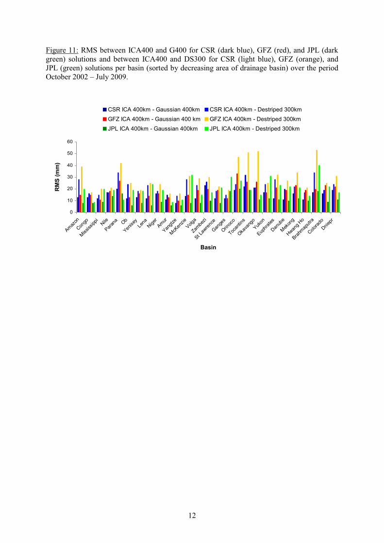
solutions are generally larger for the GFZ-based destriped solutions, especially in tropical 520
17
regions where the performances of the destriping are not the best and the hydrological signal 521
the largest (Fig. 11). 522
We present an analysis of possible sources of error on the computation of regional averages 523
versus time using the 300, 400, 500-km pre-filtered ICA solutions. This task is made on the 524
longest available period of time for each center (CSR, JPL, GFZ), and for the 27 drainage 525
basins (Table 1). 526
The formal error decreases with the number of points (see Eq. 10 and 11), the surface of the 527
considered region, and the value of error k at each grid point. In the case of the Amazon 528
Basin (~6 millions of km²), the formal error is only of 4.5 mm when k = 100 mm of 529
equivalent-water height. For the Dniepr river basin that represents the smallest surface of our 530
chosen basins (~0.52 million of km²), the formal error reaches 12.3 mm. For the series of 531
basins, the maximum values of formal errors on the regional average are in the range of 10-15 532
km3 of water volume per hundred of mm of error on the gridded points. 533
To estimate the frequency cut-off error , we made statistics of the 534
numerical tests were performed to see what maximum error can be reached using Eq. 12. We 535
computed this residual quantity for 300, 400 and 500 km-filtered ICA solutions and for each 536
hydrological basin for N1=60 and N2=300. The maximum error is always less than 1 km3, as 537
shown previously (Ramillien et al., 2006a), and it decreases with the filtering wavelength of 538
the pre-processing. In other words, this error simply increases with the level of noise in the 539
data. For the 300 km and 400 km pre-filtered solutions, the maximum values are found for the 540
Amur River: 0.3 km3 (CSR), 0.1 km
3 (JPL), and 0.8 km
3 (GFZ), and 0.04 km
3 (CSR), 0.09 541
km3 (JPL), 0.08 km
3 (GFZ) respectively. While using the 500-km filtered solutions, the error 542
of truncation is less than 0.005 km3. 543
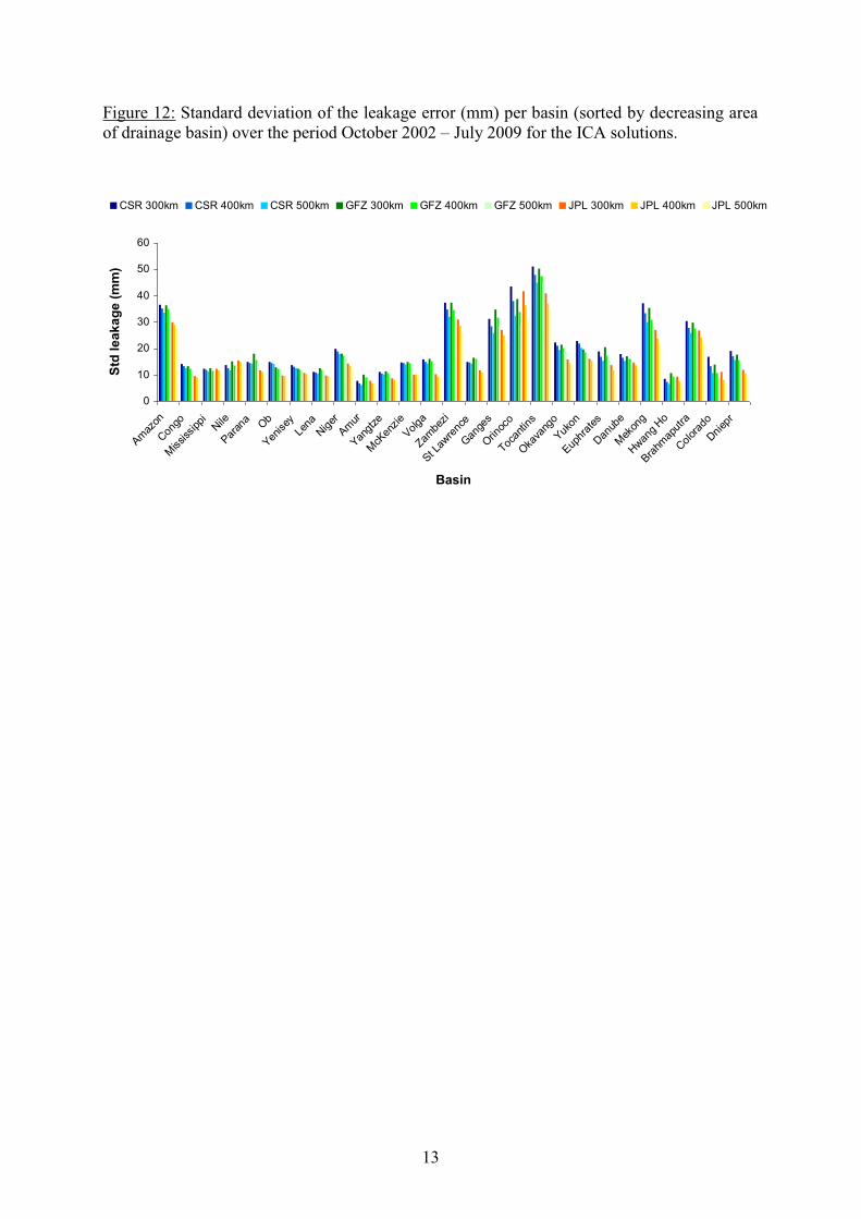
The leakage error on the ICA solutions was computed per drainage basin (see section 3.5). 544
The results are presented in Fig. 12 for the different centres and radii of Gaussian prefiltering 545
of 300, 400 and 500 km. We observed that the leakage decreases with radius of filtering and 546
is generally lower in the JPL solutions, which presents lowest peak to peak amplitudes. This 547
leakage error is logically greater in areas where several basins with large hydrological signal 548
are close, i.e., South America with the Amazon, the Parana, the Orinoco and the Tocantins, or 549
tropical Asia with the Ganges, the Brahmaputra and the Mekong rivers. The leakage error is 550
also greater for basins with small hydrological signals close to a predominant basin having 551
important hydrological variations, i.e., the Okavango and the Zambezi with the Congo. 552
553
4.4. Basin scale validation 554
18
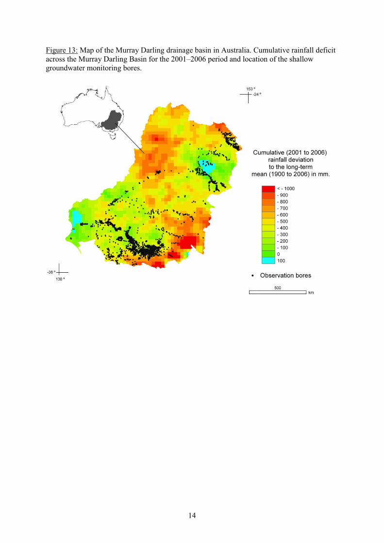
555
GRACE observations were used to estimate variations in TWS over the Murray Darling Basin 556
(see Fig. 13 for the location of the basin) at an interannual scale from January 2003 to 557
December 2008. The annual variations in TWS from GRACE for different types of solutions 558
were compared to the annual TWS computed as the sum of in situ observations (SW+GW) 559
and NOAH outputs (SM). In the Murray-Darling River basin, GLDAS-NOAH simulations of 560
SM range from 5 to 29% (in volumetric water content) across the basin for the study period, 561
and are within typical values for monthly means at 1° resolution (Lawrence and Hornberger, 562
2007). Besides, Leblanc et al. (2009) show that, between 2003 and 2007, the linear rate of 563
water changes for the GRACE TWS time series is similar to that observed for the annual total 564
water storage from in situ observations and modeling. The combined annual anomalies of 565
surface water, groundwater and soil moisture are highly correlated with the annual GRACE 566
TWS (R = 0.94 and mean absolute difference =13 km3 for the 2003 2007 period). These 567
latter interannual field-based data are considered as the reference in the following analysis. 568
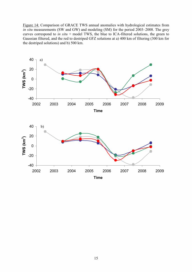
The results are presented on Fig. 14 for the GFZ solutions. The ICA solutions generally 569
present a temporal pattern closer to the so-called reference (i.e., the sum of in situ data for SW 570
and GW and model outputs for SM). This temporal pattern and the associated dynamics do 571
not change with the radius of filtering, which is not the case with the Gaussian filtered, and 572
the destriped and smoothed solutions. None of the solutions are able to retrieve the minimum 573
observed in 2007 in the reference dataset. It is important to notice that the largest part of the 574
interannual variations of TWS comes from the GW reservoir. For this hydrological 575
component, the water storage is derived from in situ measurements through Eq. (1), and is 576
highly dependent on the specific yield coefficient; where averages of local measurements are 577
used to determine ranges of regional-scale estimates. For the Murray Darling Basin, 578
composed of several aquifers, this leads to a broad range of spatial variability for the GW 579
estimates. This variability is around or greater than 20 km3 for 2002, 2007 and 2008 and 580
around 10 km3 for 2003, 5 km
3 in 2004 and 2006, 2.5 km
3 in 2005. We present yearly 581
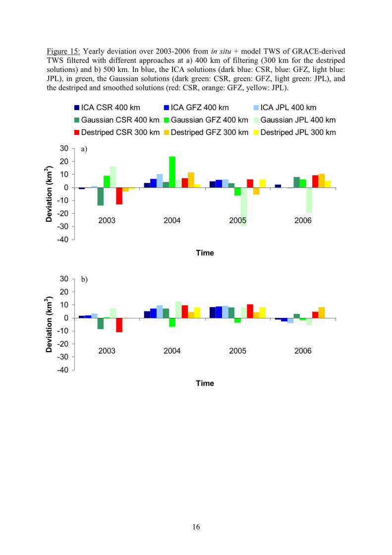
deviations to the reference for the different considered solutions (Fig. 15) over 2003-2006, 582
where the range of variability of the GW is lower. Generally, the absolute deviation of ICA-583
derived TWS to the reference is lower than 5 km3, especially for solutions filtered at 400 km. 584
At 500 km, the smoothing due to the preprocessing using a Gaussian filter is more important 585
and explains the slight increase of the absolute deviation as the spatial resolution is degraded. 586
The destriping method and the Gaussian filtering also exhibit good performances, even if 587
19
important deviations are sometimes observed (particularly with the Gaussian filter for a radius 588
of 400 km). 589
590
5. Conclusion 591
592
The ICA-based approach is a very efficient method for successfully separating TWS from 593
noise in the GRACE Level-2 data. We demonstrated that this method is more robust than 594
classical filtering methods, such as the Gaussian filtering or the destriping. Comparisons at a 595
global-scale showed that the ICA-based solutions present less north-south stripes than 596
Gaussian and destriped solutions on the land, and more realistic hydrological structures than 597
the destriped solutions in the tropics. Trend maps over 2003-2008 have also been computed. 598
The corresponding trend maps present more realistic trend patterns than those obtained with 599
other types of solutions (see for example over the Amazon and Orinoco Basins with the 400 600
km radius of prefiltering). ICA filtering seems to allow the separation of the GIA from the 601
TWS as negative trends were found over the Laurentides and Scandinavia. Unfortunately, this 602
important geophysical parameter does not appear clearly in an ICA mode yet. The major 603
drawback of this approach is that it can not directly be applied to the GRACE Level-2 raw 604
data, as a first step of prefiltering is required. In this study, we applied a Gaussian filtering 605
which deteriorates the location of the important water mass patterns. This aspect of the pre-606
treatment to be improved and highlights the necessity to replace the Gaussian filter used for 607
preprocessing the GRACE Level-2 raw data by one more suited to improve the quality of the 608
GRACE-derived TWS and thus obtain trustworthy estimate of the trends. 609
At the basin-scale, the ICA-based solutions allowed us to filter out the unrealistic peaks 610
present in the time-series of TWS obtained using classical filtering for basins with areas lower 611
than one million km². Among the ICA-based solutions, the JPL solutions are less affected by 612
leakage compared with other solutions. JPL solutions also exhibit the lowest peak-to-peak 613
amplitudes. The error balance of the GRACE-derived TWS is dominated by the effect of the 614
leakage. 615
Validation with in situ measurements was performed in the Murray Darling Basin where 616
broad networks of in situ measurements of SW and GW are available. The ICA-based 617
solutions are in better agreement with in situ data compared with the other types of solutions, 618
especially where prefiltering at a 400 km of radius. The maximum deviations are lower by a 619
factor two or three compared with the other filtering methods. 620
621
Acknowlegdements 622
20
623
This work was partly supported by the fondation Sciences et Techniques pour 624
(STAE) in the framework of the CYMENT Project (post-doctoral grant for 625
Frédéric Frappart) and the Australian Research Council grant DP0666300 (Marc Leblanc and 626
Sarah Tweed). The authors also wish to thank Dr. Matthew Rodell for his help during the 627
revision process. 628
629
References 630 631 Alsdorf, D. E., & Lettenmaier, D.P. (2003). Tracking fresh water from space. Science, 301, 632
1492-1494. 633
634
Andersen, O. B., Seneviratne, S.I., Hinderer, J. & Viterbo, P. (2005). GRACE-derived 635
terrestrial water storage depletion associated with the 2003 European heat wave, Geophysical 636
Research Letters, 32(18), L18405. 637
638
Bettadpur, S. (2007). CSR level-2 processing standards document for level-2 product release 639
0004, GRACE 327 742, Rev. 3.1. 640
641
Chambers, D.P. (2006). Evaluation of new GRACE time-variable gravity data over the ocean. 642
Geophysical Research Letters, 33, LI7603, doi:10.1029/2006GL027296. 643
644
Chen, J. L., Wilson, C. R., Tapley, B. D., Yang, Z. L. & Niu G.Y. (2009). 2005 drought event 645
in the Amazon River basin as measured by GRACE and estimated by climate models, Journal 646
of Geophysical Research, 114, B05404, doi:10.1029/2008JB006056. 647
648
Comon, P. (1994). Independent component analysis: a new concept? Signal Processing, 36, 649
287-314. 650
651
Cresswell, R.G., Dawes, W.R., Summerell, G.K., & Walker G.R. (2003). Assessment of 652
salinity management options for Kyeamba Creek, New South Wales: Data analysis and 653
groundwater modelling. CSIRO Land and Water Technical Report 26/03. 654
655
Cristescu, R., Joutsensalo, J., & Ristaniemi, T. (200). Fading Channel Estimation by Mutual 656
Information Minimization for Gaussian Stochastic Processes, Proceedings of IEEE 657
International Conference on Communications (ICC2000), New Orleans, USA, June 18-22, 658
2000, 56-59. 659
660
CSIRO (2008). Water availability in the Loddon-Avoca. A report to the Australian 661
Government from the CSIRO Murray-Darling Basin Sustainable Yields Project. CSIRO, 662
Australia. 123pp. 663
664
Davis, J.L., Tamisiea, M.E., Elósegui, P., Mitrovica, J.X., & Hill, E.M. (2008). A statistical 665
filtering approach for Gravity Recovery and Climate Experiment (GRACE) gravity data. 666
Journal Geophysical Research, 113, B04410, doi:10.1029/2007JB005043. 667
668
De Lathauwer, L., De Moor, B., & Vandewalle, J. (2000). An introduction to independent 669
component analysis. Journal of Chemometrics, 14, 123-149. 670
21
671
Ek, M. B., Mitchell, K. E., Lin, Y., Rogers, E., Grunmann, P., Koren, V., Gayno, G. & 672
Tarpley, J.D. (2003). Implementation of Noah land surface model advances in the National 673
Centers for Environmental Prediction operational mesoscale Eta model. J. Geophys. Res., 674
108(D22), 8851, doi:10.1029/2002JD003296. 675
676
Fetter, C. W. (2001). Applied Hydrogeology. 4th
ed. Prentice-Hall, New Jersey. 598 p. 677
678
Frappart, F., Ramillien, G., Biancamaria, S., Mognard, N.M. & Cazenave A. (2006). 679
Evolution of high-latitude snow mass derived from the GRACE gravimetry mission (2002-680
2004), Geophysical Research Letters, 33, L02501. 681
682
Frappart, F., Papa, F., Famiglietti, J.S., Prigent, C., Rossow, W.B. & Seyler F. (2008). 683
Interannual variations of river water storage from a multiple satellite approach: A case study 684
for the Rio Negro River basin, Journal of Geophysical Research, 113, D21104, 685
doi:10.1029/2007JD009438. 686
687
Frappart, F., Ramillien, G., Maisongrande, P., & Bonnet, M-P. (2010). Denoising satellite 688
gravity signals by Independent Component Analysis. IEEE Geosciences and Remote Sensing 689
Letters, 7(3), 421-425, doi:10.1109/LGRS.2009.2037837. 690
691
Frappart, F., Ramillien, G. & Famiglietti, J.S. (in press). Water balance of the Arctic drainage 692
system using GRACE gravimetry products. International Journal of Remote Sensing, doi: 693
10.1080/01431160903474954. 694
695
Gelle, G., Colas, M., & Serviere, C., (2001). Blind source separation: a tool for rotating 696
machine monitoring by vibration analysis ? Journal of Sound and Vibration, 248, 865-885. 697
698
Han, S-C., Shum, C.K., Jekeli, C., Kuo, C-Y., Wilson, C., & Seo K-W. (2005). Non-isotropic 699
filtering of GRACE temporal gravity for geophysical signal enhancement. Geophysical 700
Journal International, 163, 18 25. 701
702
van Hateren, J.H., & van der Schaaf, A. (1998). Independent component filters of natural 703
images compared with simple cells in primary visual cortex. Proceedings of the Biological 704
Society, 265, 359 366. 705
706
Hekmeijer P., & Dawes, W. (2003a). Assessment of salinity management options for South 707
Loddon Plains, Victoria: Data analysis and groundwater modeling. CSIRO Land and Water 708
Technical Report 24/03. 709
710
Hekmeijer P., & Dawes, W. (2003b). Assessment of salinity management options for Axe 711
Creek, Victoria: Data analysis and groundwater modelling. CSIRO Land and Water Technical 712
Report 22/03, MDBC Publication 08/03, 40pp. 713
714
Hyvärinen, A. (1999). Fast and Robust Fixed-Point Algorithms for Independent Component 715
Analysis. IEEE Transactions on Neural Networks, 10, 626-634. 716
717
Hyvärinen, A., & Oja, E. (2000). Independent Component Analysis: Algorithms and 718
Applications. Neural Networks, 13, 411-430. 719
720
22
Ife, D. & Skelt, K. (2004). Murray Darling Basin Groundwater Status 1990-2000. Murray 721
Darling Basin Commission, publication 32/04, Canberra. ISBN 1876830948. Available online 722
at http://www.mdbc.gov.au 723
724
Jekeli, C. (1981). Alternative methods to s Tech. Rep., 725
Department of Geodetic Science, Ohio State University, Colombus, Ohio. 726
727
Kirby, M., Evans, R., Walker, G., Cresswell, R., oram, S. Khan, Z. Paydar, M. Mainuddin, N. 728
McKenzie and S. Ryan (2006). The shared water resources of the Murray-Darling Basin. 729
Murray-Darling Basin Commission, Publication 21/06, Canberra. ISBN 192103887X. 730
Available online at http://www.mdbc.gov.au. 731
732
Klees, R., Revtova, E.A., Gunter, B.C., Ditmar, P., Oudman, E., Winsemius, H.C., & 733
Savenije, H.H.G. (2008). The design of an optimal filter for monthly GRACE gravity models. 734
Geophysical Journal International, 175, 417-432, doi: 10.1111/j.1365-246X.2008.03922.x. 735
736
Kusche, J. (2007). Approximate decorrelation and non-isotropic smoothing of time-variable 737
GRACE-type gravity field models. Journal of Geodesy, 81,733 749. 738
739
Lawrence, J. E., & Hornberger, G.M. (2007). Soil moisture variability across climate zones, 740
Geophysical Research Letters, 34, L20402, doi:10.1029/2007GL031382. 741
742
Leblanc, M. J., Tregoning, P., Ramillien, G., Tweed, S.O., & Fakes, A. (2009). Basin scale, 743
integrated observations of the early 21st century multiyear drought in southeast Australia. 744
Water Resources Research, 45, W04408, doi:10.1029/2008WR007333. 745
746
Macumber, P.G. (1999). Groundwater flow and resource potential in the Bridgewater and 747
Salisbury West GMAs. Phillip Macumber Consulting Services, Melbourne, 88p. 748
749
Oki, T., & Sud, Y.C. (1998). Design of Total Runoff Integrating Pathways (TRIP) - A global 750
river channel network. Earth Interactions, 2 (1), 1-37. 751
752
Paulson, A., Zhong, S. & Wahr, J. (2007). Inference of mantle viscosity from GRACE and 753
relative sea level data. Geophysical Journal International, 171 (2), 497-508. 754
755
Peltier, W.R. (2004). Global Glacial Isostasy and the Surface of the Ice-Age Earth: The ICE-756
5G(VM2) model and GRACE. Annual Review of Earth and Planetary Sciences, 32, 111-149. 757
758
Petheram, C., Dawes, W., Walker, G., Grayson, R.B. (2003). Testing in class variability of 759
groundwater systems: local upland systems. Hydrological Processes, 17, 2297-2313. 760
761
Pöyhönen, S., Jover, P., & Hyötyeniemi, H. (2003). Independent Component Analysis of 762
vibrations for fault diagnosis of an induction motor. Proceedings of the IASTED 763
International Conference on Circuits, Signal and Systems (CSS 2003), Cancun, Mexico, 19-764
21 May 2003, 1, 203-208. 765
766
Ramillien, G., Frappart, F., Cazenave, A., & Güntner, A. (2005). Time variations of land 767
water storage from the inversion of 2-years of GRACE geoids. Earth Planetary Science 768
Letters, 235, 283-301, doi:10.1016/j.epsl.2005.04.005. 769
770
23
Ramillien, G., Frappart, F., Güntner, A., Ngo-Duc, T., Cazenave, A. & Laval, K. (2006a). 771
Time-variations of the regional evapotranspiration rate from Gravimetry Recovery And 772
Climate Experiment (GRACE) satellite gravimetry. Water Resources Research, 42, W10403, 773
doi:10.1029/2005WR004331. 774
775
Ramillien, G., Lombard, A., Cazenave, A., Ivins, E.R., Llubes, M., Remy, F. & Biancale, R. 776
(2006b). Interannual variations of the mass balance of the Antarctica and Greenland ice sheets 777
from GRACE. Global and Planetary Change, 53(3), 198 208. 778
779
Ramillien, G., Famiglietti, J.S., & Wahr, J. (2008). Detection of continental hydrology and 780
glaciology signals from GRACE: a review. Surveys in Geophysics, 29, 361-374, doi: 781
10.1007/s10712-008-9048-9. 782
783
Ristaniemi, T., & Joutsensalo, J. (1999). On the Performance of Blind Symbol Separation in 784
CDMA Downlink. Proceedings of the International Workshop on Independent Component 785
Analysis and Signal Separation (ICA'99), Aussois, France, January 11-15, 1999, 437-442. 786
787
Rodell, M., Famiglietti, J.S., Chen, J., Seneviratne, S.I., Viterbo, P., Holl S. & Wilson C.R. 788
(2004a), Basin scale estimates of evapotranspiration using GRACE and other observations 789
Geophysycal Research Letters, 31(20), L20504. 790
791
Rodell, M., Houser, P. R., Jambor, U. & Gottschalck, J. (2004b). The Global Land Data 792
Assimilation System. Bulletin of the American Meteoroogical Society, 85(3), 381 394, 793
doi:10.1175/BAMS-85-3-381. 794
795
Rodell, M., Chen, J., Kato, H., Famiglietti, J.S., Nigro, J. & Wilson, C. (2007). Estimating 796
groundwater storage changes in the Mississippi River basin (USA) using GRACE. 797
Hydrogeology Journal, 15(1), 159-166. 798
799
Sasgen, I., Martinec, Z., & Fleming, K. (2006). Wiener optimal filtering of GRACE data. 800
Studia Geophysica Et Geodaetica,50, 499 508. 801
802
Schmidt, R., Flechtner, F., Meyer, U., Neumayer, K.-H., Dahle, Ch., Koenig, R., & Kusche, J. 803
(2008). Hydrological Signals Observed by the GRACE Satellites. 804
Surveys in Geophysics, 29, 319 334, doi: 10.1007/s10712-008-9033-3. 805
806
Seitz, F., Schmidt, M. & Shum, C.K. (2008). Signals of extreme weather conditions in Central 807
Europe in GRACE 4-D hydrological mass variations, Earth and Planetary Science Letters, 808
268(1-2), 165-170. 809
810
Seo, K-W., & Wilson, C.R. (2005). Simulated estimation of hydrological loads from GRACE, 811
Journal of Geodesy, 78, 442 456. 812
813
Smitt, C., Doherty, J., Dawes, W. & Walker, G. (2003). Assessment of salinity management 814
options for the Brymaroo catchment, South-eastern Queensland. CSIRO Land and Water 815
Technical Report 23/03. 816
817
Stone, J.V. (2004). Independent Component Analysis: A Tutorial Introduction, MIT Press: 818
Bradford Book. 819
820
24
Strassberg, G., Scanlon, B. R., & Rodell, M. (2007) Comparison of seasonal terrestrial water 821
storage variations from GRACE with groundwater-level measurements from the High Plains 822
Aquifer (USA). Geophysical Research Letters, 34, L14402, doi:10.1029/2007GL030139. 823
824
Swenson, S., & Wahr, J. (2006). Post-processing removal of correlated errors in GRACE 825
data, Geophysycal Research Letters, 33, L08402, doi:10.1029/2005GL025285. 826
827
Syed, T.H., Famiglietti, J.S., Chambers, D. (2009). GRACE-based estimates of terrestrial 828
freshwater discharge from basin to continental scales, Journal of Hydrometeorology, 10(1), 829
doi: 10.1175/2008JHM993.1. 830
831
Tapley, B.D., Bettadpur, S., Ries, J.C., Thompson, P.F. & Watkins M. (2004). GRACE 832
measurements of mass variability in the Earth system. Science, 305, 503-505. 833
834
Tregonning, P., Ramillien, G., McQueen, H. & Zwartz, D. (2009). Glacial isostatic 835
adjustement observed by GRACE. Journal of Geophysical Research, 114, B06406, 836
doi:10.1029/2008JB006161. 837
838
Urbano, L. D., Person, M., Kelts, K. & Hanor, J. S. (2004). Transient groundwater impacts on 839
the development of paleoclimatic lake records in semi-arid environments. Geofluids, 4, 187840
196. 841
842
Vigário, R. (1997). Extraction of ocular artifacts from EEG using independent component 843
analysis, Encephalography and Clinical Neurophysiology, 103(3), 395-404. 844
845
Tables 846
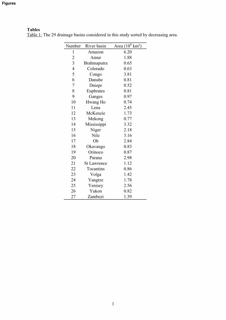
847 Table 1: The 29 drainage basins considered in this study sorted by decreasing area. 848
849
Figures 850
851 Figure 1: GRACE water storage from GFZ filtered with a Gaussian filter of 400 km of radius. 852
(Top) First ICA component corresponding to land hydrology and ocean mass. (Bottom) Sum 853
of the second and third components corresponding to the north south stripes. (a) March 2006, 854
(b) September 2006, (c) March 2007, (d) March 2008. Units are millimeters of EWT. 855
856
Figure 2: Time series of the kurtosis of the mass anomalies detected by GRACE after 857
Gaussian filtering for radii of a) 300 km, b) 400 km, c) 500 km. 858
859
Figure 3: Correlation maps over the period 2003-2008 between the ICA-filtered TWS and the 860
Gaussian-filtered TWS. Left column: ICA400-G400 (a: CSR, c: GFZ, e: JPL). Right column: 861
ICA500-G500 (b: CSR, d: GFZ, f: JPL). 862
863
Figure 4: RMS maps over the period 2003-2008 between the ICA-filtered TWS and the 864
Gaussian-filtered TWS. Left column: ICA400-G400 (a: CSR, c: GFZ, e: JPL). Right column: 865
ICA500-G500 (b: CSR, d: GFZ, f: JPL). 866
867
Figure 5: Correlation maps over the period 2003-2008 between the ICA-filtered TWS and the 868
destriped and smoothed TWS. Left column: ICA400-DS300 (a: CSR, c: GFZ, e: JPL). Right 869
column: ICA500-DS500 (b: CSR, d: GFZ, f: JPL). 870
25
871
Figure 6: RMS maps over the period 2003-2008 between the ICA-filtered TWS and the 872
destriped and smoothed TWS. Left column: ICA400-DS300 (a: CSR, c: GFZ, e: JPL). Right 873
column: ICA500-DS500 (b: CSR, d: GFZ, f: JPL). 874
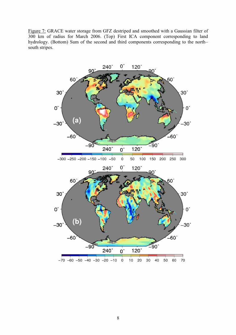
875
Figure 7: GRACE water storage from GFZ destriped and smoothed with a Gaussian filter of 876
300 km of radius for March 2006. (Top) First ICA component corresponding to land 877
hydrology. (Bottom) Sum of the second and third components corresponding to the north878
south stripes. 879
880
Figure 8: Trend maps over the period 2003-2008 of TWS using the GFZ solutions a) ICA400, 881
b) ICA500, c) G400, d) G500, e) DS300 and f) DS500. 882
883
Figure 9: Location of the 27 drainage basins chosen in this study. See Table 1 for the 884
correspondence between basins and numbers. 885
886
Figure 10: Time series of TWS (mm) derived from ICA400 (black), G400 (blue), DS300 (red) 887
for GFZ solutions over the Amazon (a), Ob (b) and Mekong (c) basins. 888
889
Figure 11: RMS between ICA400 and G400 for CSR (dark blue), GFZ (red), and JPL (dark 890
green) solutions and between ICA400 and DS300 for CSR (light blue), GFZ (orange), and 891
JPL (green) solutions per basin (sorted by decreasing area of drainage basin) over the period 892
October 2002 July 2009. 893
894
Figure 12: Standard deviation of the leakage error (mm) per basin (sorted by decreasing area 895
of drainage basin) over the period October 2002 July 2009 for the ICA solutions. 896
897
Figure 13: Map of the Murray Darling drainage basin in Australia. Cumulative rainfall deficit 898
across the Murray Darling Basin for the 2001 2006 period and location of the shallow 899
groundwater monitoring bores. 900
901
Figure 14: Comparison of GRACE TWS annual anomalies with hydrological estimates from 902
in situ measurements (SW and GW) and modeling (SM) for the period 2003 2008. The grey 903
curves correspond to in situ + model TWS, the blue to ICA-filtered solutions, the green to 904
Gaussian filtered, and the red to destriped GFZ solutions at a) 400 km of filtering (300 km for 905
the destriped solutions) and b) 500 km. 906
907
Figure 15: Yearly deviation over 2003-2006 from in situ + model TWS of GRACE-derived 908
TWS filtered with different approaches at a) 400 km of filtering (300 km for the destriped 909
solutions) and b) 500 km. In blue, the ICA solutions (dark blue: CSR, blue: GFZ, light blue: 910
JPL), in green, the Gaussian solutions (dark green: CSR, green: GFZ, light green: JPL), and 911
the destriped and smoothed solutions (red: CSR, orange: GFZ, yellow: JPL). 912
1
Tables
Table 1: The 29 drainage basins considered in this study sorted by decreasing area.
Number River basin Area (106 km²)
1 Amazon 6.20
2 Amur 1.88
3 Brahmaputra 0.65
4 Colorado 0.63
5 Congo 3.81
6 Danube 0.81
7 Dniepr 0.52
8 Euphrates 0.81
9 Ganges 0.97
10 Hwang Ho 0.74
11 Lena 2.45
12 McKenzie 1.73
13 Mekong 0.77
14 Mississippi 3.32
15 Niger 2.18
16 Nile 3.16
17 Ob 2.84
18 Okavango 0.83
19 Orinoco 0.87
20 Parana 2.98
21 St Lawrence 1.12
22 Tocantins 0.86
23 Volga 1.42
24 Yangtze 1.78
25 Yenisey 2.56
26 Yukon 0.82
27 Zambezi 1.39
Figures
2
Figures
Figure 1: GRACE water storage from GFZ filtered with a Gaussian filter of 400 km of radius
for March 2006. (Top) First ICA component corresponding to land hydrology and ocean
mass. (Bottom) Sum of the second and third components corresponding to the north south
stripes. (a) March 2006, (b) September 2006, (c) March 2007, (d) March 2008. Units are
millimeters of EWT.
March 2006 September 2006
March 2007 March 2008
a) b)
c) d)
3
Figure 2: Time series of the kurtosis of the independent components (1st and sum of 2
nd and
3rd
) of mass anomalies detected by GRACE for different radii of Gaussian filtering: a) 300
km, b) 400 km, c) 500 km.
4
Figure 3: Correlation maps over the period 2003-2008 between the ICA-filtered TWS and the
Gaussian-filtered TWS. Left column: ICA400-G400 (a: CSR, c: GFZ, e: JPL). Right column:
ICA500-G500 (b: CSR, d: GFZ, f: JPL).
a) b)
a)
c) d)
e) f)
5
Figure 4: RMS maps over the period 2003-2008 between the ICA-filtered TWS and the
Gaussian-filtered TWS. Left column: ICA400-G400 (a: CSR, c: GFZ, e: JPL). Right column:
ICA500-G500 (b: CSR, d: GFZ, f: JPL).
a) b)
c) d)
e) f)
6
Figure 5: Correlation maps over the period 2003-2008 between the ICA-filtered TWS and the
destriped and smoothed TWS. Left column: ICA400-DS300 (a: CSR, c: GFZ, e: JPL). Right
column: ICA500-DS500 (b: CSR, d: GFZ, f: JPL).
a) b)
c) d)
e) f)
7
Figure 6: RMS maps over the period 2003-2008 between the ICA-filtered TWS and the
destriped and smoothed TWS. Left column: ICA400-DS300 (a: CSR, c: GFZ, e: JPL). Right
column: ICA500-DS500 (b: CSR, d: GFZ, f: JPL).
a) b)
c) d)
e) f)
8
Figure 7: GRACE water storage from GFZ destriped and smoothed with a Gaussian filter of
300 km of radius for March 2006. (Top) First ICA component corresponding to land
hydrology. (Bottom) Sum of the second and third components corresponding to the north
south stripes.
9
Figure 8: Trend maps over the period 2003-2008 of TWS using the GFZ solutions a) ICA400,
b) ICA500, c) G400, d) G500, e) DS300 and f) DS500.
a) b)
c) d)
e) f)
10
Figure 9: Location of the 27 drainage basins chosen in this study. See Table 1 for the
correspondence between basins and numbers.
11
Figure 10: Time series of TWS (mm) derived from ICA400 (black), G400 (blue), DS300 (red)
for GFZ solutions over the Amazon (a), Ob (b) and Mekong (c) basins.
a)
b)
c)
12
Am
ur
Zambe
zi
CSR ICA 400km - Gaussian 400km CSR ICA 400km - Destriped 300km
GFZ ICA 400km - Gaussian 400 km GFZ ICA 400km - Destriped 300km
JPL ICA 400km - Gaussian 400km JPL ICA 400km - Destriped 300km
0
10
20
30
40
50
60
Am
azon
Con
go
Mississ
ippi
Nile
Par
ana
Ob
Yen
isey
Lena
Nig
er
Am
ur
Yan
gtze
McK
enzie
Volga
Zambe
zi
St L
awre
nce
Gan
ges
Orin
oco
Tocan
tins
Oka
vang
o
Yuk
on
Eup
hrat
es
Dan
ube
Mek
ong
Hwan
g Ho
Bra
hmap
utra
Col
orad
o
Dni
epr
Basin
RM
S (
mm
)Figure 11: RMS between ICA400 and G400 for CSR (dark blue), GFZ (red), and JPL (dark
green) solutions and between ICA400 and DS300 for CSR (light blue), GFZ (orange), and
JPL (green) solutions per basin (sorted by decreasing area of drainage basin) over the period
October 2002 July 2009.
13
0
10
20
30
40
50
60
Am
azon
Con
go
Mississ
ippi
Nile
Par
ana
Ob
Yen
isey
Lena
Nig
er
Am
ur
Yan
gtze
McK
enzie
Volga
Zambe
zi
St L
awre
nce
Gan
ges
Orin
oco
Tocan
tins
Oka
vang
o
Yuk
on
Eup
hrat
es
Dan
ube
Mek
ong
Hwan
g Ho
Bra
hmap
utra
Col
orad
o
Dni
epr
Basin
Std
le
ak
ag
e (
mm
)
Am
ur
Zambe
zi
CSR 300km CSR 400km CSR 500km GFZ 300km GFZ 400km GFZ 500km JPL 300km JPL 400km JPL 500km
Figure 12: Standard deviation of the leakage error (mm) per basin (sorted by decreasing area
of drainage basin) over the period October 2002 July 2009 for the ICA solutions.
14
Figure 13: Map of the Murray Darling drainage basin in Australia. Cumulative rainfall deficit
across the Murray Darling Basin for the 2001 2006 period and location of the shallow
groundwater monitoring bores.
15
Figure 14: Comparison of GRACE TWS annual anomalies with hydrological estimates from
in situ measurements (SW and GW) and modeling (SM) for the period 2003 2008. The grey
curves correspond to in situ + model TWS, the blue to ICA-filtered solutions, the green to
Gaussian filtered, and the red to destriped GFZ solutions at a) 400 km of filtering (300 km for
the destriped solutions) and b) 500 km.
-40
-20
0
20
40
2002 2003 2004 2005 2006 2007 2008 2009
Time
TW
S (
km
3)
-40
-20
0
20
40
2002 2003 2004 2005 2006 2007 2008 2009
Time
TW
S (
km
3)
a)
b)
16
Figure 15: Yearly deviation over 2003-2006 from in situ + model TWS of GRACE-derived
TWS filtered with different approaches at a) 400 km of filtering (300 km for the destriped
solutions) and b) 500 km. In blue, the ICA solutions (dark blue: CSR, blue: GFZ, light blue:
JPL), in green, the Gaussian solutions (dark green: CSR, green: GFZ, light green: JPL), and
the destriped and smoothed solutions (red: CSR, orange: GFZ, yellow: JPL).
-40
-30
-20
-10
0
10
20
30
2003 2004 2005 2006
Time
Devia
tio
n (
km
3)
ICA CSR 400 km ICA GFZ 400 km ICA JPL 400 km
Gaussian CSR 400 km Gaussian GFZ 400 km Gaussian JPL 400 km
Destriped CSR 300 km Destriped GFZ 300 km Destriped JPL 300 km
-40
-30
-20
-10
0
10
20
30
2003 2004 2005 2006
Time
Devia
tio
n (
km
3)
a)
b)


![[Hydrology] Groundwater Hydrology - David K. Todd (2005)](https://img.pdfslide.net/doc/110x75/548ce7beb47959e2288b45f9/hydrology-groundwater-hydrology-david-k-todd-2005.jpg)

![[Hydrology] groundwater hydrology david k. todd (2005)](https://img.pdfslide.net/doc/110x75/55a8e6001a28ab6c2f8b4687/hydrology-groundwater-hydrology-david-k-todd-2005-55b0d9a792c06.jpg)