Embed Size (px)
Citation preview
General rights Copyright and moral rights for the publications made accessible in the public portal are retained by the authors and/or other copyright owners and it is a condition of accessing publications that users recognise and abide by the legal requirements associated with these rights.
• Users may download and print one copy of any publication from the public portal for the purpose of private study or research. • You may not further distribute the material or use it for any profit-making activity or commercial gain • You may freely distribute the URL identifying the publication in the public portal
If you believe that this document breaches copyright please contact us providing details, and we will remove access to the work immediately and investigate your claim.
Downloaded from orbit.dtu.dk on: May 05, 2018
An Innovative Synthesis Methodology for Process Intensification
Lutze, Philip; Woodley, John; Gani, Rafiqul
Publication date:2011
Document VersionPublisher's PDF, also known as Version of record
Link back to DTU Orbit
Citation (APA):Lutze, P., Woodley, J., & Gani, R. (2011). An Innovative Synthesis Methodology for Process Intensification.Technical University of Denmark, Department of Chemical Engineering.
Philip LutzePh.D. ThesisDecember 2011
An Innovative Synthesis Metho-dology for Process Intensification
An Innovative Synthesis Methodology for
Process Intensification
Ph. D. Thesis
Philip Lutze
31 December 2011
Process Engineering and Technology Department of Chemical and Biochemical Engineering
Technical University of Denmark
1
ii
2
Copyright©: Philip Lutze
December 2011
Address: Center for Process Engineering and Technology (PROCESS)
Department of Chemical and Biochemical Engineering
Technical University of Denmark
Building 229
DK-2800 Kgs. Lyngby
Denmark
Phone: +45 4525 2800
Fax: +45 4593 2906
Web: www.process.kt.dtu.dk
Print: J&R Frydenberg A/S
København
April 2012
ISBN: 9978-87-92481-67-2
iii
Preface This thesis is submitted as partial fulfilment of the requirements for the Doctor of Philosophy (Ph.D.)
degree at the Technical University of Denmark (DTU).
The PhD-project has been carried out at the Center for Process Engineering and Technology (PROCESS)
at the Department of Chemical and Biochemical Engineering from November 2008 till December 2011
under the supervision of Professor John M. Woodley and Professor Rafiqul Gani from the Computer
Aided Process-Product Engineering Center (CAPEC). The project was partly funded by a scholarship from
the Technical University of Denmark.
First, I would like to thank my supervisors John M. Woodley and Rafiqul Gani for giving me the
opportunity to work on a very interesting and challenging project and for their valuable support,
inspiring ideas and discussions, and for their constant enthusiasm throughout my whole project.
I also would like to thank Emmanuel A. Dada from ChemProcess Technologies Inc. and the collaborators
from Argonne National Laboratory, USA for interesting project discussions and their support.
Many thanks, to all my co-workers/friends from the big “CAPEC-PROCESS-family” for providing this
wonderful atmosphere in which it is easy to work and for all the shared social events inside and outside
DTU.
Also many thanks to all my friends “outside” for their support and for the distracting discussions (mostly
about football) whenever I had the chance to meet them.
I also wish to thank my mother Gabriele, my brother Robert, and my sister Miriam for all their
encouraging words as well as for their understanding; especially in stressful times. A special thanks to
my brother Robert for giving me the idea to become a chemical engineer.
Last but for sure not least, my special thanks goes to my girlfriend Martina for the wonderful time we
share, for making me laugh, for her patience; simply for her love and her presence in my life!
Dortmund, December 2011
Philip Lutze
3

iv
4
v
Abstract Process intensification (PI) has the potential to improve existing processes or create new process
options, which are needed in order to produce products using more sustainable methods.
A variety of intensified equipment has been developed which potentially creates a large number of
options to improve a process. However, to date only a limited number have achieved implementation in
industry, such as reactive distillation, dividing wall columns and reverse flow reactors. A reason for this is
that the identification of the best PI option is neither simple nor systematic. That is to decide where and
how the process should be intensified for the biggest improvement. Until now, most PI has been
selected based on case-based trial-and-error procedures, not comparing different PI options on a
quantitative basis.
Therefore, the objective of this PhD project is to develop a systematic synthesis/design methodology to
achieve PI. It allows the quick identification of the best PI option on a quantitative basis and will push
the implementation and acceptance of PI in industry. Such a methodology should be able to handle a
large number of options. The method of solution should be efficient, robust and reliable using a well-
defined screening procedure. It should be able to use already existing PI equipment as well as to
generate novel PI equipment.
This PhD-project succeeded in developing such a synthesis/design methodology. In order to manage the
complexities involved, the methodology employs a decomposition-based solution approach. Starting
from an analysis of existing processes, the methodology generates a set of PI process options.
Subsequently, the initial search space is reduced through an ordered sequence of steps. As the search
space decreases, more process details are added, increasing the complexity of the mathematical
problem but decreasing its size. The best PI options are ordered in terms of a performance index and a
related set are verified through detailed process simulation. Two building blocks can be used for the
synthesis/design which is PI unit-operations as well as phenomena. The use of PI unit-operations as
building block aims to allow a quicker implementation/retrofit of processes while phenomena as
building blocks enable the ability to develop novel process solutions beyond those currently in
existence. Implementation of this methodology requires the use of a number of methods/algorithms,
models, databases, etc., in the different steps which have been developed. PI unit-operations are stored
and retrieved from a knowledge-base tool. Phenomena are stored and retrieved from a phenomena
library.
5

vi
The PI synthesis/design methodology has been tested for both building blocks on a number of case
studies from different areas such as conventional and bio-based bulk chemicals as well as
pharmaceuticals.
6
vii
Resume på Dansk Proces intensifikation har potentialet at forbedre eksisterende processer eller at generere nye proces
optioner, som er nødvendige til at producere produkter med hjælp af vedvarende metoder. En vifte af
intensiferet udstyr blev udviklet som potentielt skaber et stort antal af optioner at forbedre en proces.
Det er dog til dato kun en begrænset antal af implementeringer i industrien, som eksempelvis reaktiv
destillation, skillevæg kolonner og omvendt flow reaktorer. En årsag til det er at identifikationen af den
bedste PI option er ikke simple eller systematisk. Det er at beslutte, hvor og hvordan processen skal
blive intensiveret for at opnå den største forbedring. Indtil i dag de fleste PI blev udvalgt baseret på
case-baseret ”trial and error” procedurer hvilke ikke sammenligner forskellige PI optioner på et
kvantitativt grundlag. Målsætning af dette PhD projekt er derfor at udvikle en systematisk
syntese/design metodologi til at opnå PI. Det gør det muligt at hurtig identificere den bedste PI option
på et kvantitativt grundlag og vil dermed understøtte en implementering og accept af PI i industrien. En
sådan metode børe være i stand til at håndtere et stort antal af optioner. Den valgte løsning børe være
effektiv, robust og pålidelig og benytte en veldefineret screening procedure. Det bør være i stand til at
benytte eksisterende PI udstyr såvel som at generere ny PI udstyr.
Det lykkedes i dette PhD projekt at udvikle en sådan syntese/design metodologi. For at styre af
kompleksiteten metodologien benytter en nedbrydende tilgang. Startende fra en analyse af
eksisterende processer metoden generer et sæt af PI proces optioner. Efterfølgende det første søgnings
rum bliver reduceret med hjælp af en kontrolleret sekvens af trin. Med faldende størrelsen af søgnings
rum mere proces detaljer bliver tilføjet, hvilke øger kompleksiteten med henblik af den matematiske
formulering men med reducering af den reelle størrelse. De bedste PI optioner bliver arrangeret i form
af præstations indeks og en relateret sæt bliver verificeret med hjælp af detaljerede proces
simulationer.
To ”byggeklodser” kan blive benyttet til syntese/design hvilke er PI enhedsoperationer såvel som
fænomen baserede. Brugen af PI enhedsoperationer som ”byggeklodser” har som formål til at tillade en
hurtigere implementering/retrofit af processer mens fænomen baserede ”byggeklodser” giver
muligheden til at udvikle nye proces løsninger udover de nuværende eksisterende. Implementeringen af
denne metodologi kræver anvendelsen af et antal af metoder/algoritmer, modeller, databaser osv. i de
forskellige trin, hvilke blev udviklet. PI enhedsoperationer bliver gemt og hentet fra en videns baseret
værktøj. For at benytte fænomener til at syntetisere processer ”forbindelses” regler blev udviklet til at
7

viii
samle fænomener til enhedsoperationer og enhedsoperationer til processer. Fænomener bliver gemt
og hentet fra et fænomen bibliotek.
Den Pi syntese/design metode blev testet for ”byggeklodser” på et antal af casestudier fra forskellige
områder som konventionelle og bio-baseret bulk kemikalier såvel som lægemidler.
8
ix
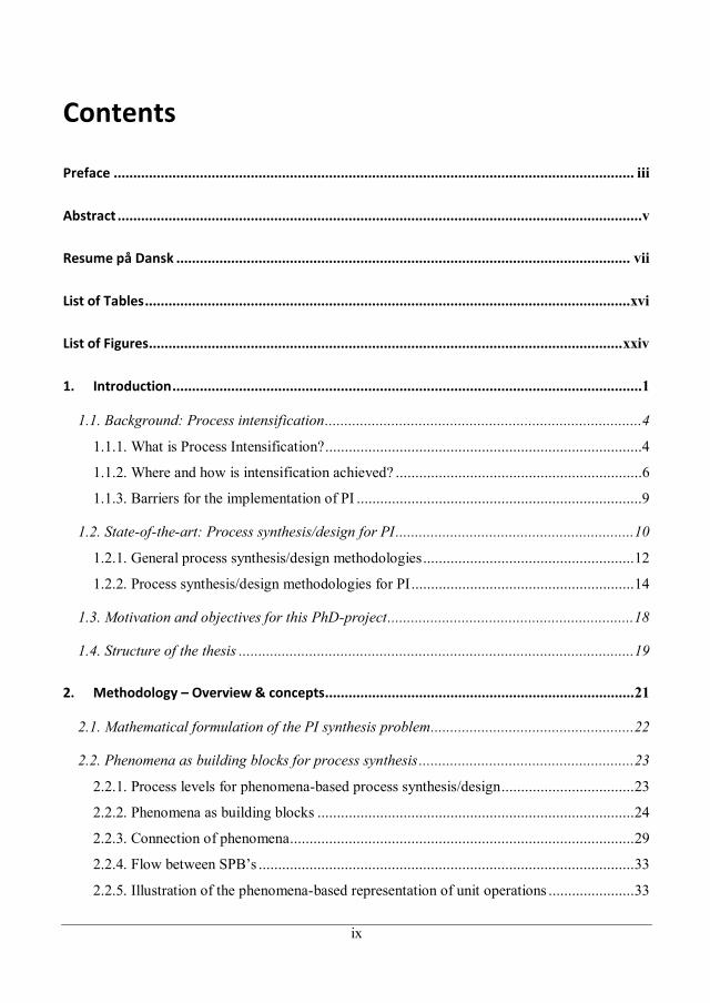
Contents
Preface ..................................................................................................................................... iii
Abstract ......................................................................................................................................v
Resume på Dansk .................................................................................................................... vii
List of Tables ............................................................................................................................xvi
List of Figures......................................................................................................................... xxiv
1. Introduction ........................................................................................................................1
1.1. Background: Process intensification .................................................................................4
1.1.1. What is Process Intensification? .................................................................................4
1.1.2. Where and how is intensification achieved? ...............................................................6
1.1.3. Barriers for the implementation of PI .........................................................................9
1.2. State-of-the-art: Process synthesis/design for PI ............................................................. 10
1.2.1. General process synthesis/design methodologies ...................................................... 12
1.2.2. Process synthesis/design methodologies for PI ......................................................... 14
1.3. Motivation and objectives for this PhD-project ............................................................... 18
1.4. Structure of the thesis ..................................................................................................... 19
2. Methodology – Overview & concepts ............................................................................... 21
2.1. Mathematical formulation of the PI synthesis problem.................................................... 22
2.2. Phenomena as building blocks for process synthesis ....................................................... 23
2.2.1. Process levels for phenomena-based process synthesis/design .................................. 23
2.2.2. Phenomena as building blocks ................................................................................. 24
2.2.3. Connection of phenomena........................................................................................ 29
2.2.4. Flow between SPB’s ................................................................................................ 33
2.2.5. Illustration of the phenomena-based representation of unit operations ...................... 33
9
x
2.3. The decomposition-approach .......................................................................................... 36
2.3.1. PI synthesis based on the decomposition-approach................................................... 37
2.4. A performance metric for PI ........................................................................................... 40
3. Methodology – Workflow ................................................................................................. 41
3.1. Workflow of the unit-operation based PI synthesis/design methodology .......................... 42
3.1.1. Brief overview of the workflow ............................................................................... 42
3.1.2. Step 1: Define problem ............................................................................................ 44
3.1.3. Step A2: Analyze the process ................................................................................... 46
3.1.4. Step B2: Identify and analyze necessary tasks to achieve the process targets ............ 49
3.1.5. Step U2: Collect PI equipment ................................................................................. 51
3.1.6. Step U3SP: Select & develop models ........................................................................ 52
3.1.7. Step U4SP: Generate feasible flowsheet options ........................................................ 53
3.1.8. Step U5SP: Fast screening for process constraints ..................................................... 53
3.1.9. Step 6: Solve the reduced optimization problem and validate promising .................. 55
3.2. Workflow of the phenomena based PI synthesis/design methodology .............................. 55
3.2.1. Brief overview of the workflow ............................................................................... 56
3.2.2. Step 1: Define problem ............................................................................................ 57
3.2.3. Step A2: Analyze the process ................................................................................... 57
3.2.4. Step B2: Identify and analyze necessary tasks to achieve the process targets ............ 57
3.2.5. Step P3: Identification of desirable phenomena ........................................................ 58
3.2.6. Step P4SP: Generate feasible operation/flowsheet options ......................................... 59
3.2.7. Step P5SP: Fast screening for process constraints ...................................................... 63
3.2.8. Step 6: Solve the reduced optimization problem and validate promising .................. 65
3.3. Sub-algorithms ............................................................................................................... 66
3.3.1. MBS (model-based search) ...................................................................................... 66
3.3.2. LBSA (limitation/bottleneck sensitivity analysis) .................................................... 66
3.3.3. APCP (analysis of pure component properties) ........................................................ 67
3.3.4. AMP (analysis of mixture properties) ...................................................................... 69
3.3.5 AR (analysis of reactions) ......................................................................................... 70
10
xi
3.3.6. OPW (operating process window) ........................................................................... 72
3.3.7. DS (development of a superstructure) ...................................................................... 72
3.3.8. SoP (selection of phenomena) .................................................................................. 73
3.3.9. AKM (apply the extended Kremser method) ........................................................... 74
3.3.10. KBS (knowledge base search)................................................................................ 75
4. Methodology – Supporting methods & tools.................................................................... 77
4.1. Knowledge-base tool ...................................................................................................... 77
4.1.1. Architecture of the knowledge-base ......................................................................... 77
4.1.2. Existing PI equipment. ............................................................................................. 78
4.1.3. Knowledge for identification of PI principles. .......................................................... 79
4.2. Model library ................................................................................................................. 81
4.3. Method based on thermodynamic insights ....................................................................... 84
4.4. Driving-Force (DF) method............................................................................................ 85
4.5. Element based approach for reactive separations ........................................................... 86
4.5.1. Calculation of the reactive bubble point ................................................................... 87
4.6. Extended Kremser Method .............................................................................................. 88
4.6.1. Derivation of the relationship between DF and Rmin to be used for the determination
of the minimum ratio R=L/V ............................................................................................. 90
4.7. Description of additional tools used................................................................................ 92
5. Case studies – Application of the unit-operation based methodology ............................. 95
5.1. Production of N-acetyl-D-neuraminic acid (Neu5Ac) ..................................................... 95
5.1.1. Base-Case Design .................................................................................................... 96
5.1.2. Non-intensified design options for the base-case design ........................................... 96
5.1.3. Step 1: Define problem ............................................................................................ 97
5.1.4. Step A2: Analyze the process ................................................................................... 98
5.1.5. Step U2: Collect PI equipment ............................................................................... 102
5.1.6. Step U3SP=1: Select & develop models ................................................................... 103
5.1.7. Step U4SP=1: Generate feasible flowsheet options ................................................... 105
11
xii
5.1.8. Step U5SP=1: Fast screening for process constraints ................................................ 107
5.1.9. Step 6: Solve the reduced optimization problem and validate promising ................ 110
5.1.10. Discussion of the results....................................................................................... 111
5.2. Production of hydrogen peroxide .................................................................................. 111
5.2.1 Introduction ............................................................................................................ 111
5.2.2 Base case design ..................................................................................................... 113
5.2.3. Step 1: Define problem .......................................................................................... 113
5.2.4. Step A2: Analyze the process ................................................................................. 115
5.2.5. Step U2: Collect PI equipment ............................................................................... 123
5.2.6. Step U3SP=1: Select and develop models ................................................................. 125
5.2.7. Step U4SP=1: Generate feasible flowsheet options ................................................... 126
5.2.8. Step U5SP=1: Fast screening for process constraints ................................................ 127
5.2.9. Step U3SP=2: Select and develop models ................................................................. 127
5.2.10. Step U4SP=2: Generate feasible flowsheet options ................................................. 130
5.2.11. Step U5SP=2: Fast screening for process constraints .............................................. 132
5.2.12. Step 6: Solve the reduced optimization problem and validate promising............... 135
5.3. Production of HMF ...................................................................................................... 138
5.3.1. State-of-the-art in the production of HMF .............................................................. 138
5.3.2. Base case design .................................................................................................... 139
5.3.3. Step 1: Define problem .......................................................................................... 140
5.3.4. Step A2: Analyze the process ................................................................................. 142
5.3.5. Step U2: Collect PI technology from Knowledge-Base .......................................... 147
5.3.6. Step U3: Select & develop models ......................................................................... 150
5.3.7. Step U4: Generate feasible flowsheet options ......................................................... 152
5.3.8. Step U5: Fast screening for process constraints ...................................................... 154
5.3.9. Step 6: Solve the reduced optimization problem and validate promising ................ 158
6. Case studies – Application of the phenomena based methodology ............................... 161
6.1. Production of isopropyl-acetate .................................................................................... 161
6.1.1. Base-Case Design .................................................................................................. 161
6.1.2. Step 1: Define problem .......................................................................................... 162
12
xiii
6.1.3. Step A2: Analyze the process ................................................................................. 163
6.1.4. Step P3: Identification of desirable phenomena ...................................................... 167
6.1.5. Step P4: Generate feasible operation/flowsheet options .......................................... 172
6.1.6. Step P5: Fast screening for process constraints ....................................................... 177
6.1.7. Step 6: Solve the reduced optimization problem and validate promising ................ 181
6.1.8. Comparison with reactive distillation ..................................................................... 183
6.2. Separation of hydrogen-peroxide and water ................................................................. 186
6.2.1. Step 1: Define problem .......................................................................................... 186
6.2.2. Step B2: Identify and analyze necessary tasks to achieve the process targets .......... 188
6.2.3. Step P3: Identification of desirable phenomena ...................................................... 192
6.2.4. Step P4: Generate feasible operation/flowsheet options .......................................... 194
6.2.5. Step P5: Fast screening for process constraints ....................................................... 197
6.2.6. Step 6: Solve the reduced optimization problem and validate promising ................ 201
6.2.7. Discussion of the influence of the pre-selection of the membrane........................... 203
6.3. Production of cyclohexanol .......................................................................................... 204
6.3.1. Brief introduction to the production of cyclohexanol .............................................. 205
6.3.2. Step 1: Define problem .......................................................................................... 206
6.3.2. Step B2: Identify and analyze necessary tasks to achieve the process targets .......... 206
6.3.3. Step P3: Identification of desirable phenomena ...................................................... 214
6.3.4. Step P4: Generate feasible operation/flowsheet options .......................................... 218
7. Discussion ....................................................................................................................... 223
8. Conclusions ..................................................................................................................... 229
8.1. Achievements ................................................................................................................ 229
8.2. Open challenges & future recommendations ................................................................. 232
Abbreviation & Nomenclature ............................................................................................... 235
References .............................................................................................................................. 239
Appendix ................................................................................................................................ 249
13
xiv
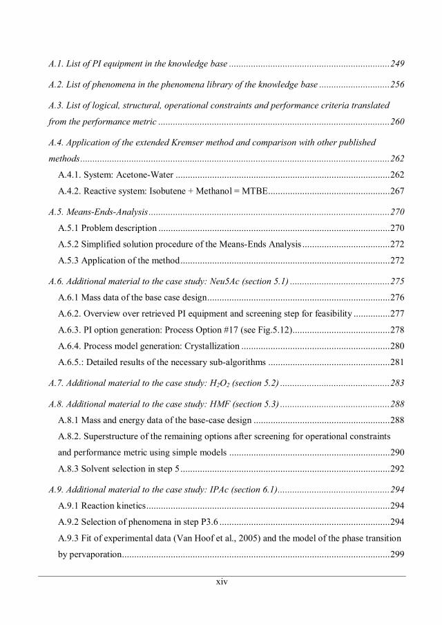
A.1. List of PI equipment in the knowledge base .................................................................. 249
A.2. List of phenomena in the phenomena library of the knowledge base ............................. 256
A.3. List of logical, structural, operational constraints and performance criteria translated
from the performance metric ............................................................................................... 260
A.4. Application of the extended Kremser method and comparison with other published
methods ............................................................................................................................... 262
A.4.1. System: Acetone-Water ........................................................................................ 262
A.4.2. Reactive system: Isobutene + Methanol = MTBE .................................................. 267
A.5. Means-Ends-Analysis ................................................................................................... 270
A.5.1 Problem description ............................................................................................... 270
A.5.2 Simplified solution procedure of the Means-Ends Analysis .................................... 272
A.5.3 Application of the method ...................................................................................... 272
A.6. Additional material to the case study: Neu5Ac (section 5.1) ......................................... 275
A.6.1 Mass data of the base case design ........................................................................... 276
A.6.2. Overview over retrieved PI equipment and screening step for feasibility ............... 277
A.6.3. PI option generation: Process Option #17 (see Fig.5.12)........................................ 278
A.6.4. Process model generation: Crystallization ............................................................. 280
A.6.5.: Detailed results of the necessary sub-algorithms .................................................. 281
A.7. Additional material to the case study: H2O2 (section 5.2) ............................................. 283
A.8. Additional material to the case study: HMF (section 5.3) ............................................. 288
A.8.1 Mass and energy data of the base-case design ........................................................ 288
A.8.2. Superstructure of the remaining options after screening for operational constraints
and performance metric using simple models .................................................................. 290
A.8.3 Solvent selection in step 5 ...................................................................................... 292
A.9. Additional material to the case study: IPAc (section 6.1) .............................................. 294
A.9.1 Reaction kinetics .................................................................................................... 294
A.9.2 Selection of phenomena in step P3.6 ...................................................................... 294
A.9.3 Fit of experimental data (Van Hoof et al., 2005) and the model of the phase transition
by pervaporation .............................................................................................................. 299
14
xv
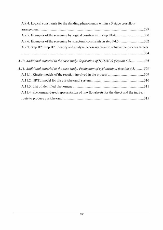
A.9.4. Logical constraints for the dividing phenomenon within a 3 stage crossflow
arrangement..................................................................................................................... 299
A.9.5. Examples of the screening by logical constraints in step P4.4 ................................ 300
A.9.6. Examples of the screening by structural constraints in step P4.5 ............................ 302
A.9.7. Step B2: Step B2: Identify and analyze necessary tasks to achieve the process targets
........................................................................................................................................ 304
A.10. Additional material to the case study: Separation of H2O2/H2O (section 6.2) .............. 305
A.11. Additional material to the case study: Production of cyclohexanol (section 6.3) ......... 309
A.11.1. Kinetic models of the reaction involved in the process ........................................ 309
A.11.2. NRTL model for the cyclohexanol system........................................................... 310
A.11.3. List of identified phenomena ............................................................................... 311
A.11.4. Phenomena-based representation of two flowsheets for the direct and the indirect
route to produce cyclohexanol ......................................................................................... 315
15
xvi
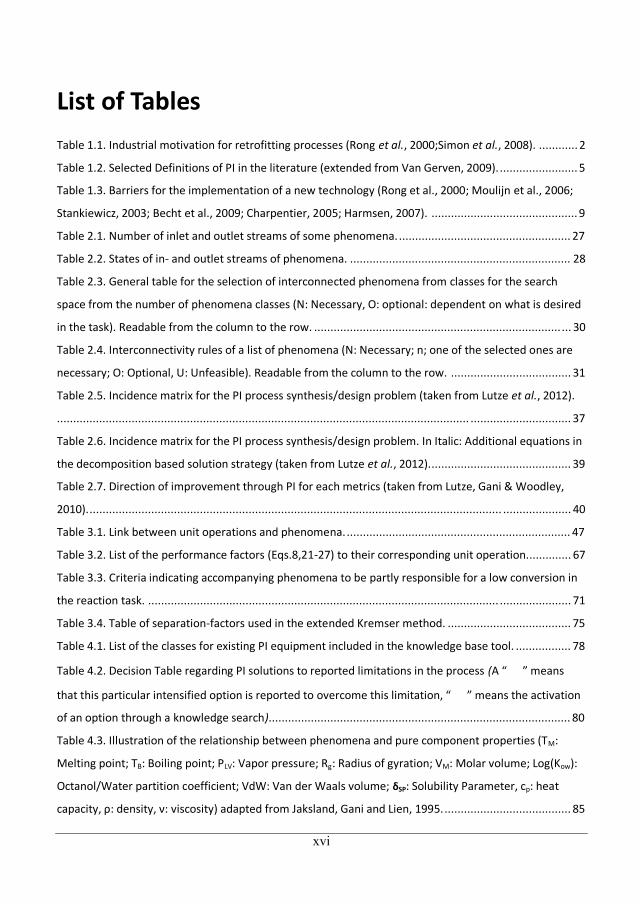
List of Tables Table 1.1. Industrial motivation for retrofitting processes (Rong et al., 2000;Simon et al., 2008). ............ 2
Table 1.2. Selected Definitions of PI in the literature (extended from Van Gerven, 2009). ........................ 5
Table 1.3. Barriers for the implementation of a new technology (Rong et al., 2000; Moulijn et al., 2006;
Stankiewicz, 2003; Becht et al., 2009; Charpentier, 2005; Harmsen, 2007). ............................................. 9
Table 2.1. Number of inlet and outlet streams of some phenomena. ..................................................... 27
Table 2.2. States of in- and outlet streams of phenomena. .................................................................... 28
Table 2.3. General table for the selection of interconnected phenomena from classes for the search
space from the number of phenomena classes (N: Necessary, O: optional: dependent on what is desired
in the task). Readable from the column to the row. ............................................................................ ... 30
Table 2.4. Interconnectivity rules of a list of phenomena (N: Necessary; n; one of the selected ones are
necessary; O: Optional, U: Unfeasible). Readable from the column to the row. ..................................... 31
Table 2.5. Incidence matrix for the PI process synthesis/design problem (taken from Lutze et al., 2012).
............................................................................................................................... ............................... 37
Table 2.6. Incidence matrix for the PI process synthesis/design problem. In Italic: Additional equations in
the decomposition based solution strategy (taken from Lutze et al., 2012). ........................................... 39
Table 2.7. Direction of improvement through PI for each metrics (taken from Lutze, Gani & Woodley,
2010). ............................................................................................................................... ..................... 40
Table 3.1. Link between unit operations and phenomena. ..................................................................... 47
Table 3.2. List of the performance factors (Eqs.8,21-27) to their corresponding unit operation.............. 67
Table 3.3. Criteria indicating accompanying phenomena to be partly responsible for a low conversion in
the reaction task. ............................................................................................................ ...................... 71
Table 3.4. Table of separation-factors used in the extended Kremser method. ...................................... 75
Table 4.1. List of the classes for existing PI equipment included in the knowledge base tool. ................. 78
Table 4.2. Decision Table regarding PI solutions to reported limitations in the process (A “ ” means
that this particular intensified option is reported to overcome this limitation, “ ” means the activation
of an option through a knowledge search)............................................................................................. 80
Table 4.3. Illustration of the relationship between phenomena and pure component properties (TM:
Melting point; TB: Boiling point; PLV: Vapor pressure; Rg: Radius of gyration; VM: Molar volume; Log(Kow):
Octanol/Water partition coefficient; VdW: Van der Waals volume; SP: Solubility Parameter, cp: heat
capacity, : density, : viscosity) adapted from Jaksland, Gani and Lien, 1995. ....................................... 85
16
xvii
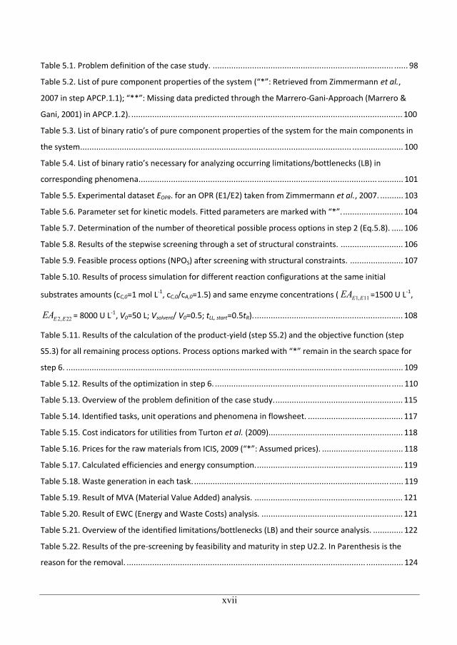
Table 5.1. Problem definition of the case study. .............................................................................. ...... 98
Table 5.2. List of pure component properties of the system (“*”: Retrieved from Zimmermann et al.,
2007 in step APCP.1.1); “**”: Missing data predicted through the Marrero-Gani-Approach (Marrero &
Gani, 2001) in APCP.1.2). ..................................................................................................................... 100
Table 5.3. List of binary ratio’s of pure component properties of the system for the main components in
the system..................................................................................................................... ...................... 100
Table 5.4. List of binary ratio’s necessary for analyzing occurring limitations/bottlenecks (LB) in
corresponding phenomena. ...................................................................................................... ........... 101
Table 5.5. Experimental dataset EOPR. for an OPR (E1/E2) taken from Zimmermann et al., 2007. .......... 103
Table 5.6. Parameter set for kinetic models. Fitted parameters are marked with “*”. .......................... 104
Table 5.7. Determination of the number of theoretical possible process options in step 2 (Eq.5.8). ..... 106
Table 5.8. Results of the stepwise screening through a set of structural constraints. ........................... 106
Table 5.9. Feasible process options (NPOS) after screening with structural constraints. ....................... 107
Table 5.10. Results of process simulation for different reaction configurations at the same initial
substrates amounts (cC,0=1 mol L-1, cC,0/cA,0=1.5) and same enzyme concentrations ( 1, 11E EEA =1500 U L-1,
2, 22E EEA = 8000 U L-1, V0=50 L; Vsolvent/ V0=0.5; tLL, start=0.5tR). ................................................................ 108
Table 5.11. Results of the calculation of the product-yield (step S5.2) and the objective function (step
S5.3) for all remaining process options. Process options marked with “*” remain in the search space for
step 6. ....................................................................................................................... .......................... 109
Table 5.12. Results of the optimization in step 6. ............................................................................ ..... 110
Table 5.13. Overview of the problem definition of the case study. ....................................................... 115
Table 5.14. Identified tasks, unit operations and phenomena in flowsheet. ......................................... 117
Table 5.15. Cost indicators for utilities from Turton et al. (2009).......................................................... 118
Table 5.16. Prices for the raw materials from ICIS, 2009 (“*”: Assumed prices). ................................... 118
Table 5.17. Calculated efficiencies and energy consumption. ............................................................... 119
Table 5.18. Waste generation in each task. .................................................................................... ...... 119
Table 5.19. Result of MVA (Material Value Added) analysis. ................................................................ 121
Table 5.20. Result of EWC (Energy and Waste Costs) analysis. ............................................................. 121
Table 5.21. Overview of the identified limitations/bottlenecks (LB) and their source analysis. ............. 122
Table 5.22. Results of the pre-screening by feasibility and maturity in step U2.2. In Parenthesis is the
reason for the removal. ....................................................................................................... ................ 124
17
xviii
Table 5.23. Specific surface area’s a for different reactor internals (from Eigenberger, 1992, Reitzmann,
Bareiss & Kraushaar-Czarnetzki, 2006) used in the catalytic hydrogenation (“*” from Goor, Glenneberg &
Jacobi, 2007). ............................................................................................................................... ....... 126
Table 5.24. Results of the calculation of Fobj for different hydrogenation reactors. ............................... 127
Table 5.25. Mass transfer coefficients kLa in s-1 for different reactors for air-water (from Yue et al., 2007,
Voigt & Schügerl, 1979 and Reay, Ramshaw & Harvey, 2009) used in the oxidation. ............................ 129
Table 5.26. Determination of the number of theoretical possible process options in step C2 (Eq. 5.24).
............................................................................................................................... ............................. 130
Table 5.27. The number of process options remaining in the search space (BCD: Base case design; W:
water; WS: working solution; PR: product rich; P: product). ................................................................. 131
Table 5.28. Results of the stepwise screening through a set of structural constraints........................... 132
Table 5.29. Calculation of the performance of the oxidation task (RM: raw material). ......................... 133
Table 5.30. Calculation of the objective function for all remaining options in SP=2 (BCD: base case
design). ...................................................................................................................... ......................... 134
Table 5.31. Calculation of the objective function for all remaining options. ......................................... 137
Table 5.32. Reported process routes (extended from Boisen et al., 2009). Conversion and selectivity are
molar based. .................................................................................................................. ..................... 139
Table 5.33. Problem definition of the case study. ............................................................................. ... 142
Table 5.34. Link between unit operations and phenomena. ................................................................. 143
Table 5.35. Cost indicators for utilities from Turton et al. (2009) and prices for the raw materials from
ICIS, 2009 (“*”:Sino Chemical Industry Co Ltd, 2010; “**” estimated price from price for acetic acid to be
0.7 US-$/kg (ICIS, 2009)). ..................................................................................................................... 144
Table 5.36. Results of the calculation of the operating costs, the energy consumption and the waste
generation in the base case design. ........................................................................................... .......... 144
Table 5.37. Results of the Material Value Added (MVA) and Energy and Waste Costs (EWC) analysis. .. 145
Table 5.38. List of the pure component properties of the key components for the system HMF (The data
with a star are predicted using the Marrero-Gani-approach (Marrero & Gani, 1997). .......................... 146
Table 5.39. Overview of the identified limitations/bottlenecks and their source analysis. .................... 146
Table 5.40. Pre-Screening of PI equipments by pure component properties. ....................................... 147
Table 5.41. Results of the pre-screening by feasibility and maturity in step U2.2. In Parenthesis is the
reason for the removal. ....................................................................................................... ................ 149
18
xix
Table 5.42. Simple models based on conversions and selectivities from the literature (1: Roman-Leshkov,
Chheda, Dumesic, 2006; 2: Tuercke, Panic & Loebbecke, 2009; *: assumed to minimum as good as the
reactor-extractor). ........................................................................................................... .................... 150
Table 5.43. Reaction parameters. .............................................................................................. .......... 151
Table 5.44. Results of the stepwise screening through a set of logical constraints. ............................... 153
Table 5.45. Results of the stepwise screening through a set of structural constraints........................... 153
Table 5.46. Process options (NPOS) after structural constraints. Abbreviations: reactive extractor (RE),
reactor (R), heat-integrated distillation column (HiDC),filter of acids and humins (Filter),
Purification(Purif). .......................................................................................................... ..................... 154
Table 5.47. Process options (NPOO) after performance screening using simple models. Abbreviations:
reactive extractor (RE), reactor (R), heat-integrated distillation column (HiDC), Filter of acids and humins
(Filter), Purification(Purif).; “*”: kept in the search space. ................................................................ .... 155
Table 5.48. Process options (NPOO) after performance screening using complex models. Abbreviations:
reactive extractor (RE), reactor (R), heat-integrated distillation column (HiDC), Filter of acids and humins
(Filter), Purification(Purif).; “*”: kept in the search space.................................................................. ... 156
Table 5.49. Ranking of the remaining process options by their objective function (Treaction=180°C; ncat=0.1
mol/kg HMF; 50 w.% fructose in the inlet; TInlet streams=40°C ). ............................................................... 158
Table 6.1. Base-Case-Design of the reactor to produce isopropyl-acetate. ........................................... 162
Table 6.2. Problem definition of the case study: IPAc. ........................................................................ .. 163
Table 6.3. List of pure component properties of the system at P=1atm (“*”:Missing data predicted
through the Marrero-Gani-Approach (Marrero & Gani, 2001) in the tool ProPred in step APCP.1.2). ... 165
Table 6.4. List of the binary ratio of some pure components properties. .............................................. 165
Table 6.5. List of the of the identified azeotropes in the mixture at p=1atm (Min.BP=Low boiling
azeotrope). Compositions are given in mol. .................................................................................... ..... 165
Table 6.6. Operating window for the temperature of both phenomena responsible for the operating
boundary of the 1-phase CSTR. ............................................................................................................ 166
Table 6.7. Decision Table regarding PI solutions to reported limitations in the process (A “ ” in the
second section means that this particular intensified option is reported to overcome this limitation,
“ ” means the activation of an option through a knowledge search) ................................................ 167
Table 6.8. Table Identified phenomena for each desirable task using the algorithm APCP and AMP (A:
Acetic-Acid, B: Isopropanol, C: Water, D: Isopropyl-acetate) with pure component properties (TM:
19
xx
Melting point; TB: Boiling point; PLV: Vapor pressure; Rg: Radius of gyration; VM: Molar volume; Log(Kow):
Octanol/Water partition coefficient; VdW: Van der Waals volume; SP: Solubility Parameter).............. 169
Table 6.9. Result of the screening of phenomena for each desirable task using the algorithm SoP (A:
Acetic-Acid, B: Isopropanol, C: Water, D: Isopropyl-acetate). The remaining phenomena and tasks which
are kept in the search space are written in bold. ............................................................................. .... 170
Table 6.10. Operating windows for involved phenomena (Assumption: P=1 atm). ............................... 172
Table 6.11. List of feasible SPB’s. The flow mixing contains the tubular as well as the rectangular flow
pattern. ...................................................................................................................... ......................... 174
Table 6.12. Results of the performance calculation of connected stages for different flow configurations.
First number is the conversion while the second number indicates the number of stages necessary to
achieve that conversion. ...................................................................................................... ................ 175
Table 6.13. Overview of the search space reduction through screening by logical constraints. ............. 176
Table 6.14. Overview of the search space reduction through screening by structural constraints......... 176
Table 6.15. Excerpt of the screening by operational constraints (yield). ............................................... 177
Table 6.16. Excerpt of the performance screening by the thermal energy consumption....................... 177
Table 6.17. Remaining process option after screening by process constraints in step P5.2. .................. 178
Table 6.18. Results for screening of operational constraints at the unit operational level. Process option
10,12 and 22 have been simulated for 100 parallel reactors. For these, in parenthesis, the volume of a
single reactor is given. The rectangular channel is assumed to have a ratio of Width/Height=1 ........... 180
Table 6.19. Simulation results for two points for both remaining process option #10 and #22 for a
number of 100 reactors in parallel. ........................................................................................... ........... 182
Table 6.20. Mass and energy data of the reactive distillation configuration (Lai et al., 2007) ................ 185
Table 6.21. Problem definition of the case study: separation of H2O2/H2O . ......................................... 188
Table 6.22. Normal property ratios of the components H2O2/H2O involved in the separation task. ...... 189
Table 6.23. Identified phenomena for each desirable task using the algorithm APCP with pure
component properties (TM: Melting point; TB: Boiling point; PLV: Vapor pressure; Rg: Radius of gyration;
VM: Molar volume; Log(Kow): Octanol/Water partition coefficient; VdW: Van der Waals volume; SP:
Solubility Parameter) ......................................................................................................... .................. 189
Table 6.24. Operating window of the phase transition phenomena with respect to temperatures. ...... 190
Table 6.25. Overview of the screening of phase transition phenomena. Kept phase transition
phenomena in the search space are written in bold letters. ................................................................. 191
Table 6.26. Operating windows for involved phenomena. ................................................................... 193
20
xxi
Table 6.27. Feasible stages based on the phenomena in the search space. .......................................... 195
Table 6.28. Number of stages to achieve the purity of H2O2 at L/Vmin/1.1. ............................................ 196
Table 6.29. Number of stages to achieve the recovery (purity of H2O) at 1.5*L/Vmin. ............................ 196
Table 6.30. Reduction of the search space by structural screening. ...................................................... 197
Table 6.31. Cost indicators for utilities from Turton et al. (2009).......................................................... 198
Table 6.32. Cost Ranking of the stripping configurations by the CostStrip. .............................................. 198
Table 6.33. Remaining process options in the search space after screening of the number of equipments
at the unit operational level. ................................................................................................ ............... 200
Table 6.34. Simulation results of each option.................................................................................. ..... 201
Table 6.35. Ranking of the remaining options by Fobj. ........................................................................... 201
Table 6.36. Comparison of process options with membranes and the best option from step 6.3. ........ 204
Table 6.37. Assignment of function of components in the system. ....................................................... 206
Table 6.38. Extended assignment of function of components in the system. ........................................ 207
Table 6.39. Calculated heat of reactions. ..................................................................................... ........ 208
Table 6.40. Equilibrium constants and conversion of the three reactions. ............................................ 208
Table 6.41. List of pure component properties. ................................................................................ ... 210
Table 6.42. Identified phenomena for each task using the algorithm APCP. ......................................... 211
Table 6.43. List of pure component boiling points and binary azeotropes at p=1 atm. ......................... 212
Table 6.44. List of necessary tasks and identified desirable tasks. ........................................................ 214
Table 6.45. Decision Table regarding PI solutions to reported limitations in the process (A “ ” in the
second section means that this particular intensified option is reported to overcome this limitation, “ ”
means the activation of an option through a knowledge search). ........................................................ 215
Table 6.46. Necessary tasks and examples of identified phenomena fulfilling them. ............................ 216
Table 6.47. Operating windows for involved phenomena (The description of phenomena behind the
abbreviation can be seen in appendix A.11.4). ................................................................................. .... 217
Table 6.48. Example of feasible SPB’s based on the phenomena in the search space. .......................... 219
Table A.1. List of PI equipment in the knowledge base. ........................................................................ 250
Table A.2. List of intensified internals in the knowledge base............................................................... 253
Table A.3. List of additional PI beyond equipment/internals in the knowledge base............................. 254
Table A.4. Detailed example of the PI knowledge base (“***”: not shown data). ................................. 255
Table A.5. List of phenomena in the phenomena library. ..................................................................... 257
21
xxii
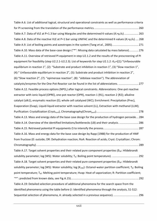
Table A.6. List of additional logical, structural and operational constraints as well as performance criteria
for PI screening from the translation of the performance metrics. ....................................................... 260
Table A.7. Data of VLE at P=1.3 bar using Margules and the determined K-values (Ki=yi/xi) .................. 263
Table A.8. Data of the reactive VLE at P=1 bar using UNIFAC and the determined K-values (Ki=yi/xi) .... 268
Table A.9. List of boiling points and azeotropes in the system (Tang et al., 2005). ................................ 271
Table A.10. Mass data of the base-case design (“*”: Missing data calculated by mass balance)............ 276
Table A.11. Overview of retrieved PI equipment in step U2.1.2 and the results of the prescreening of PI
equipment for feasibility (step U2.2.1-U2.2.3). List of keywords for step U2.1.2: KPI={(1):“Unfavourable
equilibrium in reaction 1”, (2): “Substrate and product inhibition in reaction 1”, (3):“Slow reaction 1”,
(4):“ Unfavourable equilibrium in reaction 2”, (5): Substrate and product inhibition in reaction 2”,
(6):“Slow reaction 2”, (7): “epimerase reaction”, (8): “aldolase reaction”}. The abbreviation of
catalysts/enzymes for the One-Pot-Reactor can be found in the list of abbreviations. ......................... 277
Table A.12. Feasible process options (NPOL) after logical constraints. Abbreviations: One-pot reactive
extractor with ionic liquid (OPRE), one-pot reactor (OPR), reaction 1 (R1), reaction 2 (R2); alkaline
catalyst (alk1), enzymatic reaction (E); whole cell catalyzed (WC); Enrichment: Precipitation (Prec),
Evaporation (Evap), Liquid-liquid extractor with reactive solvent (LL), Extraction with methanol (LLM);
Purification: Crystallization (CrystPurif), Chromatography(Chrompurif). .................................................... 278
Table A.13. Mass and energy data of the base case design for the production of hydrogen peroxide. .. 284
Table A.14. Overview of the identified limitations/bottlenecks (LB) and their analysis. ........................ 286
Table A.15. Retrieved potential PI equipments to intensify the process. ........................................... 287
Table A.16. Mass and energy data for the base case design by Rapp (1988) for the production of HMF
from fructose (0: outside; DR: Dehydration reaction; RoA: Reaction of acids; Cryst: Crystallizer; Chrom:
Chromatography). .............................................................................................................. ................. 289
Table A.17. Target solvent properties and their related pure component properties ( SP: Hildebrandt
solubility parameter; log (WS): Water solubility; TB: Boiling point temperature). ................................. 292
Table A.18. Target solvent properties and their related pure component properties ( SP: Hildebrandt
solubility parameter; log (WS): Water solubility; log (KOW): Octanol-water partition coefficient; TB: Boiling
point temperature; TM: Melting point temperature; Hvap: Heat of vaporization; R: Partition coefficient;
“*”: predicted from known data, see Fig.A.15).................................................................................. ... 292
Table A.19: Detailed selection procedure of additional phenomena for the search space from the
identified phenomena using the table before (I: Identified phenomena through the analysis, S1-S12:
Sequential selection of phenomena, A: already selected in a previous sequence). ............................... 296
22
xxiii
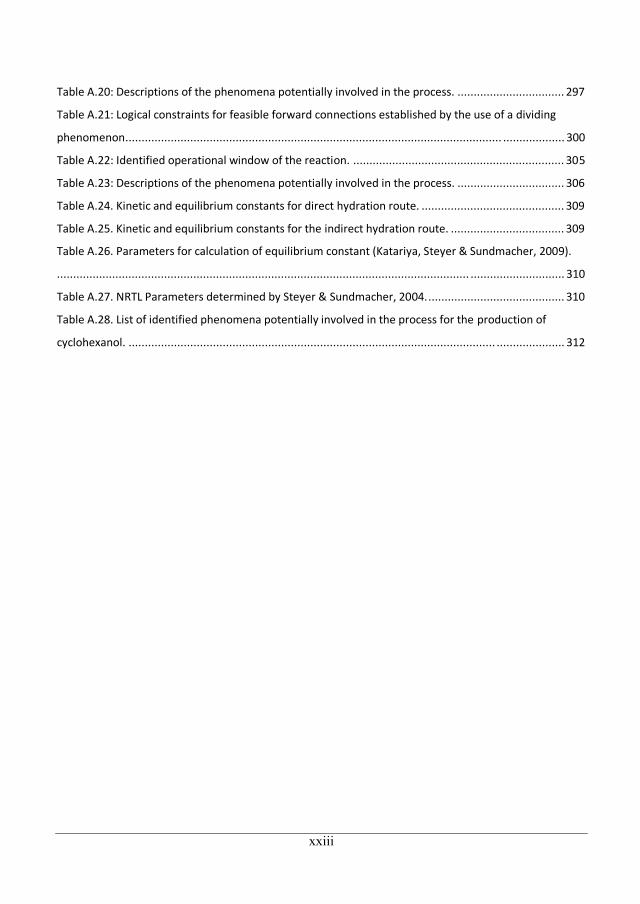
Table A.20: Descriptions of the phenomena potentially involved in the process. ................................. 297
Table A.21: Logical constraints for feasible forward connections established by the use of a dividing
phenomenon .................................................................................................................... ................... 300
Table A.22: Identified operational window of the reaction. ................................................................. 305
Table A.23: Descriptions of the phenomena potentially involved in the process. ................................. 306
Table A.24. Kinetic and equilibrium constants for direct hydration route. ............................................ 309
Table A.25. Kinetic and equilibrium constants for the indirect hydration route. ................................... 309
Table A.26. Parameters for calculation of equilibrium constant (Katariya, Steyer & Sundmacher, 2009).
............................................................................................................................... ............................. 310
Table A.27. NRTL Parameters determined by Steyer & Sundmacher, 2004. .......................................... 310
Table A.28. List of identified phenomena potentially involved in the process for the production of
cyclohexanol. ................................................................................................................. ..................... 312
23
xxiv
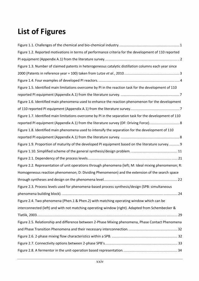
List of Figures Figure 1.1. Challenges of the chemical and bio-chemical industry. ........................................................... 1
Figure 1.2. Reported motivations in terms of performance criteria for the development of 110 reported
PI equipment (Appendix A.1) from the literature survey. ....................................................................... .. 2
Figure 1.3. Number of claimed patents in heterogeneous catalytic distillation columns each year since
2000 (Patents in reference year = 100) taken from Lutze et al., 2010. ...................................................... 3
Figure 1.4. Four examples of developed PI reactors. ........................................................................... ..... 4
Figure 1.5. Identified main limitations overcome by PI in the reaction task for the development of 110
reported PI equipment (Appendix A.1) from the literature survey. .......................................................... 7
Figure 1.6. Identified main phenomena used to enhance the reaction phenomenon for the development
of 110 reported PI equipment (Appendix A.1) from the literature survey................................................. 7
Figure 1.7. Identified main limitations overcome by PI in the separation task for the development of 110
reported PI equipment (Appendix A.1) from the literature survey (DF: Driving Force). ............................. 8
Figure 1.8. Identified main phenomena used to intensify the separation for the development of 110
reported PI equipment (Appendix A.1) from the literature survey. .......................................................... 8
Figure 1.9. Proportion of maturity of the developed PI equipment based on the literature survey. .......... 9
Figure 1.10. Simplified scheme of the general synthesis/design problem. .............................................. 11
Figure 2.1. Dependency of the process levels................................................................................... ...... 21
Figure 2.2. Representation of unit operations through phenomena (left; M: Ideal mixing phenomenon; R:
Homogeneous reaction phenomenon; D: Dividing Phenomenon) and the extension of the search space
through syntheses and design on the phenomena level. ........................................................................ 22
Figure 2.3. Process levels used for phenomena-based process synthesis/design (SPB: simultaneous
phenomena building block). .................................................................................................... .............. 24
Figure 2.4. Two phenomena (Phen.1 & Phen.2) with matching operating window which can be
interconnected (left) and with not matching operating window (right). Adapted from Schembecker &
Tlatlik, 2003. ............................................................................................................................... ........... 29
Figure 2.5. Relationship and difference between 2-Phase Mixing phenomena, Phase Contact Phenomena
and Phase Transition Phenomena and their necessary interconnection. ................................................ 32
Figure 2.6. 2-phase mixing flow characteristics within a SPB. ................................................................. 32
Figure 2.7. Connectivity options between 2-phase SPB’s. ....................................................................... 33
Figure 2.8. A fermentor in the unit-operation based representation. ..................................................... 34
24
xxv
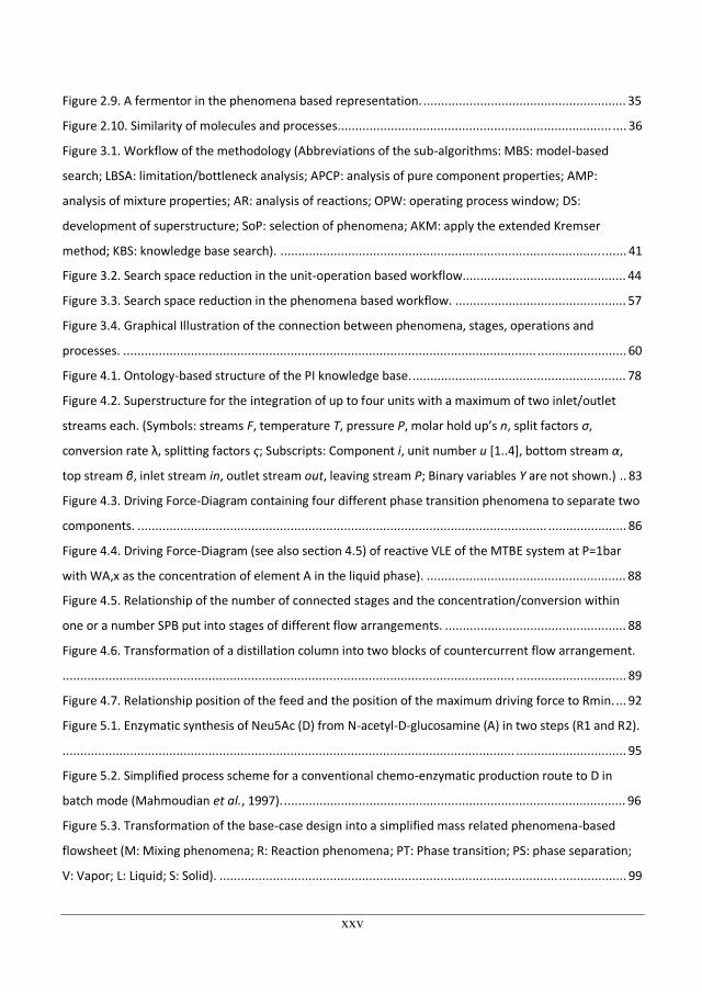
Figure 2.9. A fermentor in the phenomena based representation. ......................................................... 35
Figure 2.10. Similarity of molecules and processes............................................................................. .... 36
Figure 3.1. Workflow of the methodology (Abbreviations of the sub-algorithms: MBS: model-based
search; LBSA: limitation/bottleneck analysis; APCP: analysis of pure component properties; AMP:
analysis of mixture properties; AR: analysis of reactions; OPW: operating process window; DS:
development of superstructure; SoP: selection of phenomena; AKM: apply the extended Kremser
method; KBS: knowledge base search). ................................................................................................. 41
Figure 3.2. Search space reduction in the unit-operation based workflow.............................................. 44
Figure 3.3. Search space reduction in the phenomena based workflow. ................................................ 57
Figure 3.4. Graphical Illustration of the connection between phenomena, stages, operations and
processes. .................................................................................................................... ......................... 60
Figure 4.1. Ontology-based structure of the PI knowledge base. ............................................................ 78
Figure 4.2. Superstructure for the integration of up to four units with a maximum of two inlet/outlet
streams each. (Symbols: streams F, temperature T, pressure P, molar hold up’s n, split factors ,
conversion rate , splitting factors ; Subscripts: Component i, unit number u [1..4], bottom stream ,
top stream , inlet stream in, outlet stream out, leaving stream P; Binary variables Y are not shown.) .. 83
Figure 4.3. Driving Force-Diagram containing four different phase transition phenomena to separate two
components. ................................................................................................................... ...................... 86
Figure 4.4. Driving Force-Diagram (see also section 4.5) of reactive VLE of the MTBE system at P=1bar
with WA,x as the concentration of element A in the liquid phase). ........................................................ 88
Figure 4.5. Relationship of the number of connected stages and the concentration/conversion within
one or a number SPB put into stages of different flow arrangements. ................................................... 88
Figure 4.6. Transformation of a distillation column into two blocks of countercurrent flow arrangement.
............................................................................................................................... ............................... 89
Figure 4.7. Relationship position of the feed and the position of the maximum driving force to Rmin. ... 92
Figure 5.1. Enzymatic synthesis of Neu5Ac (D) from N-acetyl-D-glucosamine (A) in two steps (R1 and R2).
............................................................................................................................... ............................... 95
Figure 5.2. Simplified process scheme for a conventional chemo-enzymatic production route to D in
batch mode (Mahmoudian et al., 1997). ................................................................................................ 96
Figure 5.3. Transformation of the base-case design into a simplified mass related phenomena-based
flowsheet (M: Mixing phenomena; R: Reaction phenomena; PT: Phase transition; PS: phase separation;
V: Vapor; L: Liquid; S: Solid). ............................................................................................... ................... 99
25
xxvi
Figure 5.4. Comparison of the kinetic model (Eqs.5.6-5.7) with experimental data from Zimmermann et
al., 2007. ............................................................................................................................... .............. 105
Figure 5.5. Simplified flowsheet of the PI process option #17. ............................................................. 110
Figure 5.6. Dependence of the explosion range from the temperature and concentration of H2O2 in the
liquid phase at P=1atm (left) and on the total pressure and the concentration of H2O2 in the vapor
phase (right) from Goor, Glenneberg & Jacobi (2007). ......................................................................... 112
Figure 5.7. Main reactions (5.9-5.10) to produce hydrogen peroxide via the anthraquinone route. Top:
Hydrogenation (Eq.5.9); Bottom: Oxidation (Eq.5.10). ......................................................................... 112
Figure 5.8. Simplified base-case design for the production of H2O2 by the anthraquinone-route. ......... 113
Figure 5.9. Task-based representation of the base-case design for the production of H2O2 by the
anthraquinone-route. .......................................................................................................... ................ 116
Figure 5.10. Contribution to the objective function. .......................................................................... ... 120
Figure 5.11. Contribution to the energy consumption. ......................................................................... 120
Figure 5.12. Heat integrated distillation column. ............................................................................. .... 136
Figure 5.13. Simplified production route of HMF from fructose through a water route (Rapp, 1987). .. 140
Figure 5.14. The remaining process option from the superstructure for the integration of up to four units
with a maximum of two inlet/outlet streams each. (Symbols: streams F, splitting factors ; Binary
variables Y are not shown). The large arrow show where the different solvents are considered through
the superstructure............................................................................................................. .................. 157
Figure 5.15. Distribution of the costs of the best option. ..................................................................... 159
Figure 6.1. The base-case-design of a CSTR with a cooling jacket in the unit-operation-, task- and
phenomena-based flowsheet (Phenomena: M: Ideal mixing (L-phase), R: pseudohomogenous reaction,
C: Cooling; Components in bold: A: HOAc, B: IPOH, C: H2O, D: IPAc). ................................................... 164
Figure 6.2. Ternary LLE diagrams of this system at P 1bar. (NRTL model with parameters from Lai et al.,
2007). ............................................................................................................................... ................... 166
Figure 6.3. Identified tasks to overcome the limitation in the reaction. ................................................ 168
Figure 6.4. Different flow patterns for the liquid flow. ......................................................................... 171
Figure 6.5. Existing forward connections enabled through the use of a dividing phenomenon within the
3-stage crossflow stage connection superstructure. ............................................................................ 175
Figure 6.6. Identified unit operations (Red: Heat addition; Green: phase transition by pervaporation;
Yellow: no reaction)........................................................................................................... .................. 179
26
xxvii
Figure 6.7. The Pareto-Curve of the 2 best options at a yield=0.99 and 100 parallel units. Both lines are
overlapping. .................................................................................................................. ...................... 181
Figure 6.8. Detailed design of the tubular plate-frame-flow reactor-pervaporator. .............................. 182
Figure 6.9. Detailed design of the rectangular plate-frame-flow reactor-pervaporator
(Width/Height=W/H=1). ......................................................................................................... ............. 182
Figure 6.10. Base-case design for the production of IPAc (Corrigan and Stichweh, 1968). .................... 183
Figure 6.11. Reactive-distillation-stripper configuration for the production of IPAc (Lai et al, 2007).
Colorized is the reactive zone containing Amberlyst-15. ...................................................................... 184
Figure 6.12. Comparison of the design for the production of 46.5 kmol/h IPAC in the criteria conversion,
heat and amount of catalyst. .................................................................................................. ............. 186
Figure 6.13. Identified tasks to achieve the process specifications. ...................................................... 189
Figure 6.14. Identified Plot of driving force for the phase transition by relative volatility (UNIQUAC model
with parameters from the Pro\II database version 8.1 (Pro\II, 2011)) at 3 pressures and by pervaporation
at P=1 bar. ................................................................................................................... ........................ 191
Figure 6.15. Simplified superstructure of a counter-current arrangement of four stages. ..................... 196
Figure 6.16. Process option #2 at the phenomena level (left) and at the unit operation level (right). ... 202
Figure 6.17. Driving Force of phase transition by relative volatility at different pressure and by
pervaporation at different selectivities. ..................................................................................... .......... 203
Figure 6.18. Asahi process for cyclohexanol production via direct hydration of cyclohexene (Mitsui &
Fukuoka, 1984). ............................................................................................................... .................... 205
Figure 6.19. Task based flowsheet connecting inlets to the corresponding reactions. .......................... 207
Figure 6.20. Relationship of the reaction rate per kg catalyst over the temperature for the three
reactions. .................................................................................................................... ........................ 209
Figure 6.21. Task based flowsheet connecting inlets to the corresponding reactions and introducing
outlet specifications. ........................................................................................................ ................... 209
Figure 6.22. Task LLE for ternary system of cyclohexene – cyclohexanol – water simulated with NRTL
model (from Steyer & Sundmacher, 2004) for T=323 K and P=1 atm. ................................................... 213
Figure 6.23. Generic column superstructure. ....................................................................................... 220
Figure 6.24. Flowsheet for direct hydration based on unit operations (left; Steyer, Qi & Sundmacher,
2002) and based on phenomena here represented by the tasks (right). ............................................... 221
27
xxviii
Figure 6.25. Flowsheet for indirect hydration via formic acid ester based on unit operations (top;
Katariya, Steyer & Sundmacher, 2007) and based on phenomena here represented by the tasks (below).
............................................................................................................................... ............................. 222
Figure 7.1. Context of the developed synthesis/design methodology (unit-operation based approach and
phenomena-based approach) within other synthesis/design methodologies for PI. ............................. 225
Figure 7.2. Search space reduction by the decomposition approach exemplary shown for the case
studies Neu5Ac (top) and IPAc (bottom). ....................................................................................... ...... 226
Figure 8.1. Proposed framework for implementation of the methodology into a software (here shown
within the ICAS environment (Gani et al., 1997)). ................................................................................ 233
Figure A.1. Determination of Nmin by the McCabe-Thiele-Method starting from the distillate
specification. ................................................................................................................ ....................... 264
Figure A.2. Transformation of the distillation problem into two sections for the use of the Kremser-
equations. .................................................................................................................... ....................... 265
Figure A.3. Driving Force-Diagram of Acetone-Water at P=1.3bar using the Margules equation with
parameters from the ICAS database. ............................................................................................ ....... 265
Figure A.4. System description and transformation of the distillation problem into two sections for the
use of the Kremser-equations. ................................................................................................. ............ 267
Figure A.5. Driving Force-Diagram of reactive VLE of the MTBE system at P=1bar. ............................... 269
Figure A.6. Base Case Design for the production of methyl acetate (Sundmacher & Kienle, 2003). ....... 271
Figure A.7. Task based representation for the production of methyl acetate (RV: Relative volatility; in
bold: allowed in and outlet streams of the system). ........................................................................... .. 272
Figure A.8. Task based representation of the Base Case Design for the production of methyl acetate (in
bold: allowed in and outlet streams of the system). ........................................................................... .. 273
Figure A.9. Task based representation after alternative task identification for the production of methyl
acetate (in bold: allowed in and outlet streams of the system). ........................................................... 273
Figure A.10. Task based representation after task synergy identification for the production of methyl
acetate (in bold: allowed in and outlet streams of the system). ........................................................... 274
Figure A.11. Task-based and unit operation-based representation for the production of methyl acetate
(in bold: allowed in and outlet streams of the system). ....................................................................... . 275
Figure A.12. Fitting curve of experimental values (•) obtained from Mahmoudian et al. (1997) for the
crystallization separation factor of component D (on addition of five volumes of acetic acid to aqueous
solutions) depending on the concentration of D in solution. ................................................................ 281
28
xxix
Figure A.13. The five remaining process options after screening by operational constraints and
performance metrics using simple models from the superstructure for the integration of up to four units
with a maximum of two inlet/outlet streams each. (Symbols: streams F, splitting factors ; Binary
variables Y are not shown). The large arrow shows where the four different superstructures are enabled
(selection of unit in task 1 and the selection for a recycle of fructose or not. In case of the microchannel
reactor the recycle is necessary). ............................................................................................ ............. 291
Figure A.14. High boiling solvent C7H11BrCl4 (left) and low boiling solvent C5H9BrO (right) for the
extraction of HMF from an aqueous phase. ...................................................................................... ... 293
Figure A.15. Relationship of the deviation from the Hildebrandt solubility parameter of the solvents from
the solute (HMF) and the partition coefficient R. ............................................................................. .... 293
Figure A.16. Different flow patterns for the liquid flow. ..................................................................... .. 299
Figure A.17. Example for logical constraint: formation of product. ....................................................... 300
Figure A.18. Example for logical constraint: no separation of raw materials. ........................................ 301
Figure A.19. Example for logical constraint: Feasibility of connected streams. ..................................... 301
Figure A.20. Example for structural constraint: Remove energy redundant options. ............................ 302
Figure A.21. Example for structural constraint: Phenomena not linked to improve the yield. ............... 303
Figure A.22. Example for structural constraint: Remove options which potentially decrease the efficiency
in the last step. ............................................................................................................. ....................... 303
Figure A.23. Example for structural constraint: Realization in 1 unit operation possible. ...................... 304
Figure A.24. Result of step B2.3.4 which is the identification of the desired reaction task and the
corresponding reactants. ...................................................................................................... ............... 305
Figure A.25. Extended task-based flowsheet after step B2.3.6 giving the potential outlet of the system.
............................................................................................................................... ............................. 305
Figure A.26. Comparison of experimental (Steyer & Sundmacher, 2004) and simulated VLE data for the
binary pair cyclohexene (1) - cyclohexanol (2) at p=1 atm. ................................................................... 311
Figure A.27. Phenomena-based flowsheet for the direct hydration route via reactive distillation. ....... 315
Figure A.28. Phenomena-based flowsheet for the indirect hydration route via two integrated reactive
distillations. ................................................................................................................ ......................... 316
29

xxx
30
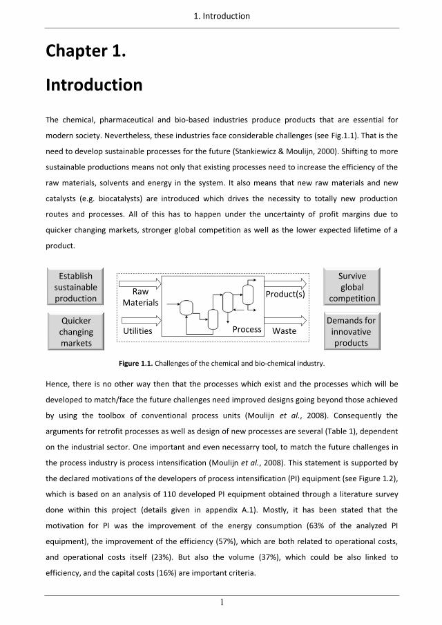
1. Introduction
1
Chapter 1.
Introduction
The chemical, pharmaceutical and bio-based industries produce products that are essential for
modern society. Nevertheless, these industries face considerable challenges (see Fig.1.1). That is the
need to develop sustainable processes for the future (Stankiewicz & Moulijn, 2000). Shifting to more
sustainable productions means not only that existing processes need to increase the efficiency of the
raw materials, solvents and energy in the system. It also means that new raw materials and new
catalysts (e.g. biocatalysts) are introduced which drives the necessity to totally new production
routes and processes. All of this has to happen under the uncertainty of profit margins due to
quicker changing markets, stronger global competition as well as the lower expected lifetime of a
product.
Establish sustainable production
Quicker changing markets
Demands for innovative products
Survive global
competition
Process
Product(s)
Waste
Raw Materials
Utilities
Figure 1.1. Challenges of the chemical and bio-chemical industry.
Hence, there is no other way then that the processes which exist and the processes which will be
developed to match/face the future challenges need improved designs going beyond those achieved
by using the toolbox of conventional process units (Moulijn et al., 2008). Consequently the
arguments for retrofit processes as well as design of new processes are several (Table 1), dependent
on the industrial sector. One important and even necessarry tool, to match the future challenges in
the process industry is process intensification (Moulijn et al., 2008). This statement is supported by
the declared motivations of the developers of process intensification (PI) equipment (see Figure 1.2),
which is based on an analysis of 110 developed PI equipment obtained through a literature survey
done within this project (details given in appendix A.1). Mostly, it has been stated that the
motivation for PI was the improvement of the energy consumption (63% of the analyzed PI
equipment), the improvement of the efficiency (57%), which are both related to operational costs,
and operational costs itself (23%). But also the volume (37%), which could be also linked to
efficiency, and the capital costs (16%) are important criteria.
31
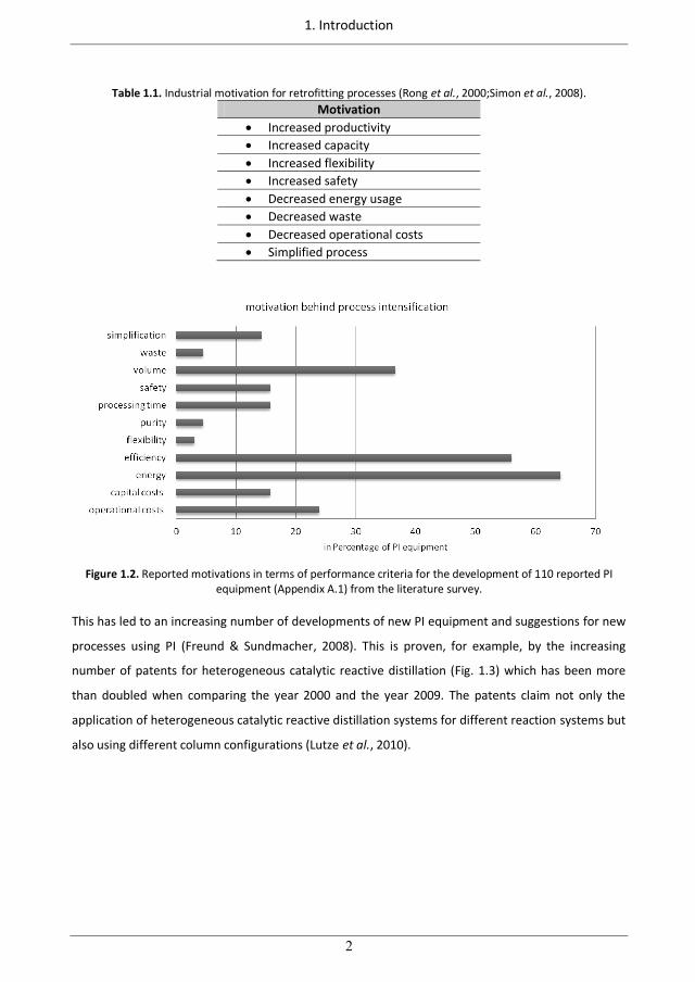
1. Introduction
2
Table 1.1. Industrial motivation for retrofitting processes (Rong et al., 2000;Simon et al., 2008). Motivation
Increased productivity Increased capacity Increased flexibility Increased safety Decreased energy usage Decreased waste Decreased operational costs Simplified process
Figure 1.2. Reported motivations in terms of performance criteria for the development of 110 reported PI
equipment (Appendix A.1) from the literature survey.
This has led to an increasing number of developments of new PI equipment and suggestions for new
processes using PI (Freund & Sundmacher, 2008). This is proven, for example, by the increasing
number of patents for heterogeneous catalytic reactive distillation (Fig. 1.3) which has been more
than doubled when comparing the year 2000 and the year 2009. The patents claim not only the
application of heterogeneous catalytic reactive distillation systems for different reaction systems but
also using different column configurations (Lutze et al., 2010).
32
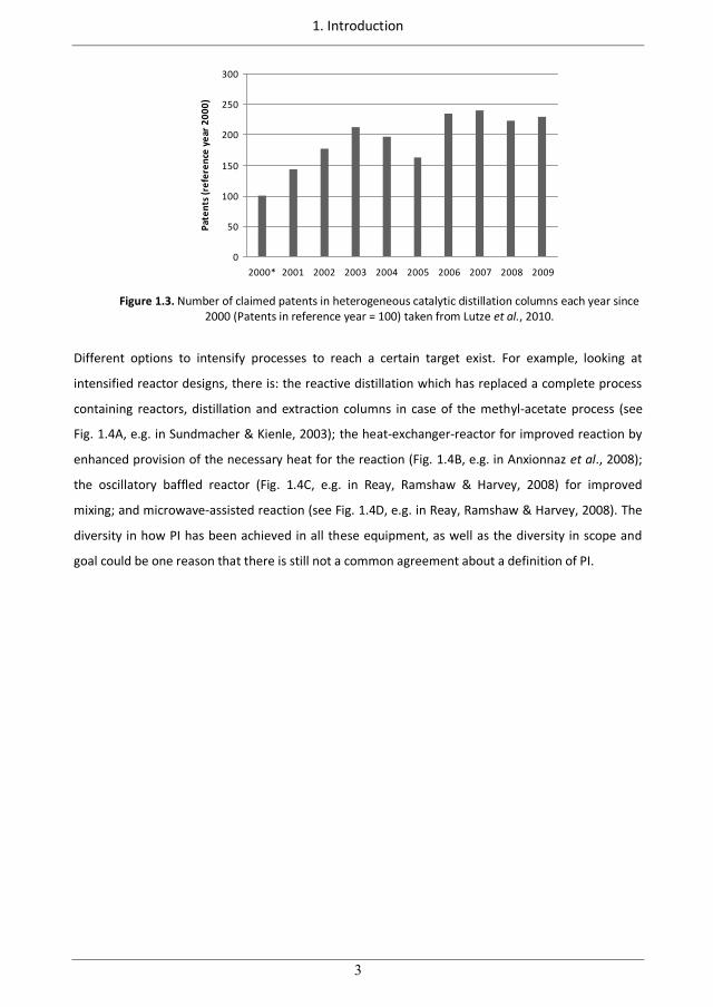
1. Introduction
3
0
50
100
150
200
250
300
2000* 2001 2002 2003 2004 2005 2006 2007 2008 2009
Pate
nts (
refe
renc
e ye
ar 2
000)
Figure 1.3. Number of claimed patents in heterogeneous catalytic distillation columns each year since
2000 (Patents in reference year = 100) taken from Lutze et al., 2010.
Different options to intensify processes to reach a certain target exist. For example, looking at
intensified reactor designs, there is: the reactive distillation which has replaced a complete process
containing reactors, distillation and extraction columns in case of the methyl-acetate process (see
Fig. 1.4A, e.g. in Sundmacher & Kienle, 2003); the heat-exchanger-reactor for improved reaction by
enhanced provision of the necessary heat for the reaction (Fig. 1.4B, e.g. in Anxionnaz et al., 2008);
the oscillatory baffled reactor (Fig. 1.4C, e.g. in Reay, Ramshaw & Harvey, 2008) for improved
mixing; and microwave-assisted reaction (see Fig. 1.4D, e.g. in Reay, Ramshaw & Harvey, 2008). The
diversity in how PI has been achieved in all these equipment, as well as the diversity in scope and
goal could be one reason that there is still not a common agreement about a definition of PI.
33
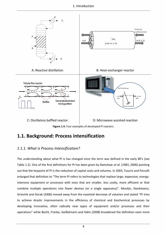
1. Introduction
4
B
A
C
D
A: Reactive distillation B: Heat-exchanger-reactor
C: Oscillatory baffled reactor D: Microwave assisted reaction
Figure 1.4. Four examples of developed PI reactors.
1.1. Background: Process intensification
1.1.1. What is Process Intensification?
The understanding about what PI is has changed since the term was defined in the early 80’s (see
Table 1.2). One of the first definitions for PI has been given by Ramshaw et al. (1983, 2000) pointing
out that the keypoint of PI is the reduction of capital costs and volumes. In 2003, Tsouris and Porcelli
enlarged that definition to “The term PI refers to technologies that replace large, expensive, energy-
intensive equipment or processes with ones that are smaller, less costly, more efficient or that
combine multiple operations into fewer devices (or a single apparatus)”. Moulijn, Stankiewicz,
Grievink and Gorak (2006) moved away from the essential decrease of volumes and stated “PI tries
to achieve drastic improvements in the efficiency of chemical and biochemical processes by
developing innovative, often radically new types of equipment and/or processes and their
operations” while Becht, Franke, Geißelmann and Hahn (2008) broadened the definition even more
34
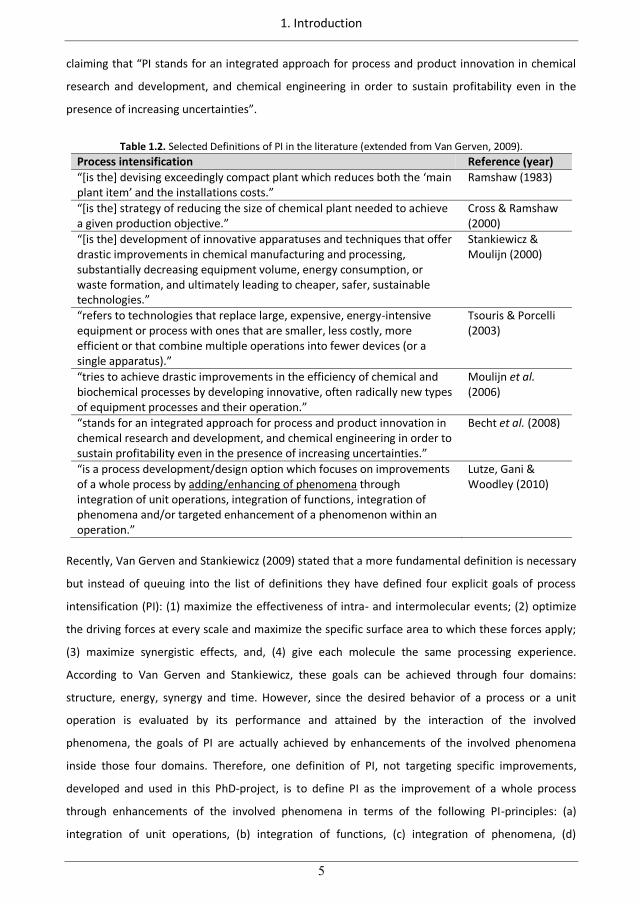
1. Introduction
5
claiming that “PI stands for an integrated approach for process and product innovation in chemical
research and development, and chemical engineering in order to sustain profitability even in the
presence of increasing uncertainties”.
Table 1.2. Selected Definitions of PI in the literature (extended from Van Gerven, 2009).
Process intensification Reference (year) “[is the] devising exceedingly compact plant which reduces both the ‘main plant item’ and the installations costs.”
Ramshaw (1983)
“[is the] strategy of reducing the size of chemical plant needed to achieve a given production objective.”
Cross & Ramshaw (2000)
“[is the] development of innovative apparatuses and techniques that offer drastic improvements in chemical manufacturing and processing, substantially decreasing equipment volume, energy consumption, or waste formation, and ultimately leading to cheaper, safer, sustainable technologies.”
Stankiewicz & Moulijn (2000)
“refers to technologies that replace large, expensive, energy-intensive equipment or process with ones that are smaller, less costly, more efficient or that combine multiple operations into fewer devices (or a single apparatus).”
Tsouris & Porcelli (2003)
“tries to achieve drastic improvements in the efficiency of chemical and biochemical processes by developing innovative, often radically new types of equipment processes and their operation.”
Moulijn et al. (2006)
“stands for an integrated approach for process and product innovation in chemical research and development, and chemical engineering in order to sustain profitability even in the presence of increasing uncertainties.”
Becht et al. (2008)
“is a process development/design option which focuses on improvements of a whole process by adding/enhancing of phenomena through integration of unit operations, integration of functions, integration of phenomena and/or targeted enhancement of a phenomenon within an operation.”
Lutze, Gani & Woodley (2010)
Recently, Van Gerven and Stankiewicz (2009) stated that a more fundamental definition is necessary
but instead of queuing into the list of definitions they have defined four explicit goals of process
intensification (PI): (1) maximize the effectiveness of intra- and intermolecular events; (2) optimize
the driving forces at every scale and maximize the specific surface area to which these forces apply;
(3) maximize synergistic effects, and, (4) give each molecule the same processing experience.
According to Van Gerven and Stankiewicz, these goals can be achieved through four domains:
structure, energy, synergy and time. However, since the desired behavior of a process or a unit
operation is evaluated by its performance and attained by the interaction of the involved
phenomena, the goals of PI are actually achieved by enhancements of the involved phenomena
inside those four domains. Therefore, one definition of PI, not targeting specific improvements,
developed and used in this PhD-project, is to define PI as the improvement of a whole process
through enhancements of the involved phenomena in terms of the following PI-principles: (a)
integration of unit operations, (b) integration of functions, (c) integration of phenomena, (d)
35
1. Introduction
6
targeted enhancements of phenomena in a given operation (Lutze, Gani & Woodley, 2010). The
advantage of this definition is that it is fundamental and it links the performance (process)
improvement to the enhanced phenomena and to the principles (and phenomena) responsible for it.
PI equipment illustrating this definition are presented in Figure 1.4. Consider the operation of a fast
and highly exothermic reaction run in a flow reactor, which is limited by mass and heat transfer
phenomena to remove the heat of reaction. The operating window of this reaction is limited to a
certain temperature region and therefore, the process is not able to achieve the goal of complete
conversion. Employing the first PI principle (a), the reaction can be enhanced through integration
with the downstream process for separation of the product (in-situ product removal to drive the
reaction to completion). In addition, the heat of reaction may be used to drive the separation.
Suitable PI equipment for this case would be a reactive distillation (Fig. 1.4A). By applying principle
(b), similar goals could be achieved through the integration of improved heating functions in the
reactor, for example a HEX Reactor (Fig. 1.4B). The improvement could also be realized through PI
principle (c), by, for example, the integration of a turbulent mixing phenomenon with the existing
flow, reaction and heating phenomena in the reactor. Insertion of baffles inside the tube together
with the oscillating (instead of continuous) pumping of the liquid through the flow reactor would
enable turbulent mixing to be created without increasing the flow velocity. This technique is actually
realized in an oscillatory baffled reactor (Fig.1.4C). Finally, PI could be achieved via principle (d)
through the application of novel forms of energy, such as microwaves, to enhance the heat transfer
or to change the reactor operation from meso-scale to micro-scale leading to enhanced mass and
heat transfer (Fig.1.4D).
1.1.2. Where and how is intensification achieved?
The focus of PI has been mostly on improvement in the reaction and the separation tasks. This trend
is not surprising since the cores of process design are the selection of the reactor and the
downstream processing (Douglas, 1985). By optimizing/improving the reactor performance, it is
possible to achieve significantly enhanced throughput or better efficiency/use of the raw materials
and also sometimes to reduce the quantity and quality of the downstream processing. But what are
the drivers behind the intensification, namely the limitations that must be overcome through the
intensification.
For the reaction task, six main limitations have been identified (Fig 1.5), namely: limitations due to
physical boundaries (such as unfavorable equilibrium, low selectivity, limited heat transfer and high
36
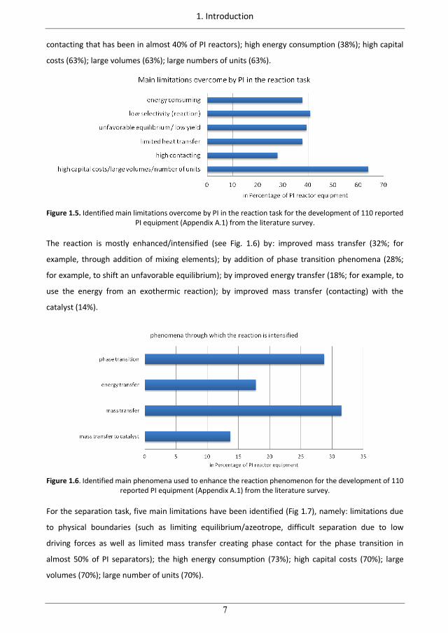
1. Introduction
7
contacting that has been in almost 40% of PI reactors); high energy consumption (38%); high capital
costs (63%); large volumes (63%); large numbers of units (63%).
Figure 1.5. Identified main limitations overcome by PI in the reaction task for the development of 110 reported
PI equipment (Appendix A.1) from the literature survey. The reaction is mostly enhanced/intensified (see Fig. 1.6) by: improved mass transfer (32%; for
example, through addition of mixing elements); by addition of phase transition phenomena (28%;
for example, to shift an unfavorable equilibrium); by improved energy transfer (18%; for example, to
use the energy from an exothermic reaction); by improved mass transfer (contacting) with the
catalyst (14%).
Figure 1.6. Identified main phenomena used to enhance the reaction phenomenon for the development of 110
reported PI equipment (Appendix A.1) from the literature survey. For the separation task, five main limitations have been identified (Fig 1.7), namely: limitations due
to physical boundaries (such as limiting equilibrium/azeotrope, difficult separation due to low
driving forces as well as limited mass transfer creating phase contact for the phase transition in
almost 50% of PI separators); the high energy consumption (73%); high capital costs (70%); large
volumes (70%); large number of units (70%).
37
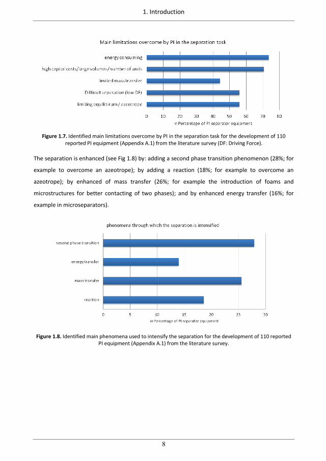
1. Introduction
8
Figure 1.7. Identified main limitations overcome by PI in the separation task for the development of 110
reported PI equipment (Appendix A.1) from the literature survey (DF: Driving Force).
The separation is enhanced (see Fig 1.8) by: adding a second phase transition phenomenon (28%; for
example to overcome an azeotrope); by adding a reaction (18%; for example to overcome an
azeotrope); by enhanced of mass transfer (26%; for example the introduction of foams and
microstructures for better contacting of two phases); and by enhanced energy transfer (16%; for
example in microseparators).
Figure 1.8. Identified main phenomena used to intensify the separation for the development of 110 reported
PI equipment (Appendix A.1) from the literature survey.
38
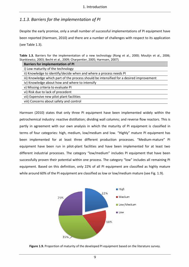
1. Introduction
9
1.1.3. Barriers for the implementation of PI
Despite the early promise, only a small number of successful implementations of PI equipment have
been reported (Harmsen, 2010) and there are a number of challenges with respect to its application
(see Table 1.3).
Table 1.3. Barriers for the implementation of a new technology (Rong et al., 2000; Moulijn et al., 2006; Stankiewicz, 2003; Becht et al., 2009; Charpentier, 2005; Harmsen, 2007).
Barriers for implementation of PI i) Low maturity of the technology ii) Knowledge to identify/decide when and where a process needs PI iii) Knowledge which part of the process should be intensified for a desired improvement iv) Knowledge about how and where to intensify v) Missing criteria to evaluate PI vi) Risk due to lack of precedent vii) Expensive new pilot plant facilities viii) Concerns about safety and control
Harmsen (2010) states that only three PI equipment have been implemented widely within the
petrochemical industry: reactive distillation; dividing wall columns; and reverse flow reactors. This is
partly in agreement with our own analysis in which the maturity of PI equipment is classified in
terms of four categories: high, medium, low/medium and low. “Highly” mature PI equipment has
been implemented for at least three different production processes. “Medium-mature” PI
equipment have been run in pilot-plant facilities and have been implemented for at least two
different industrial processes. The category “low/medium” includes PI equipment that have been
successfully proven their potential within one process. The category “low” includes all remaining PI
equipment. Based on this definition, only 22% of all PI equipment are classified as highly mature
while around 60% of the PI equipment are classified as low or low/medium mature (see Fig. 1.9).
Figure 1.9. Proportion of maturity of the developed PI equipment based on the literature survey.
39
1. Introduction
10
An example for highly mature PI equipment is reactive distillation, which has been implemented into
several industrial processes such as methyl-acetate, MTBE and others (Lutze et al., 2010). An
example for a medium mature process is the hybrid configuration of reactive distillation with a
pervaporation, which has been studied in research widely but implementation into the industry is
still scarce. An example for a low/medium mature PI equipment is the HIGee Reactor (Ramshaw,
1983) while an example for low maturity is the application of microwaves for enhancements of
reaction and separation.
Additionally, the application of “mature” technology has been limited with respect to diversity of the
processes. One example is the application of heterogeneous catalytic distillation (HeCD) which has
been analyzed based on patents concerning reaction systems and reaction characteristics
(equilibrium, kinetics, heat of reaction) as well as configurations within the column and their
integration with other units (Lutze et al., 2010). HeCD has been mostly implemented within the
petrochemical industry and for esterifications, etherification, alkylations and hydrogenation
reactions. Current development shows the application of HeCD within those reactions to higher
carbon numbers but these are probably not the only classes of reactions where HeCD might be
advantageous or most advantageously applied (Lutze et al., 2010). Furthermore, external or internal
integration of HeCD with other unit operations such as pervaporation (Buchaly, Kreis & Gorak, 2007)
or distillation (Arpornwichanop Koomsup & Assabumrungrat, 2008) or by using dividing wall column
technology (Kaibel et al., 2005) has not been reported for industrial application (Lutze et al., 2010).
1.2. State-of-the-art: Process synthesis/design for PI
In general, the identification of a feasible (and optimal) process flowsheet to convert a raw material
and necessary utilities (such as energy utilities, solvents, membranes, etc.) to the final product and
waste (see Figure 1.10) is not an easy and intuitive part (Douglas, 1985). One of the reasons is that a
large number of process options and a number of different utilities are potentially available as well
as a number of decision criteria (operational constraints, performance constraints) need to be
matched. Therefore, from the process systems engineering (PSE) toolbox, process synthesis tries to
attack those issues and difficulties within the flowsheet synthesis/design. Process synthesis involves
the identification of the optimal path to reach a desired product from a given starting point, of the
desired quality and quantity, and subject to defined constraints on the process.
40
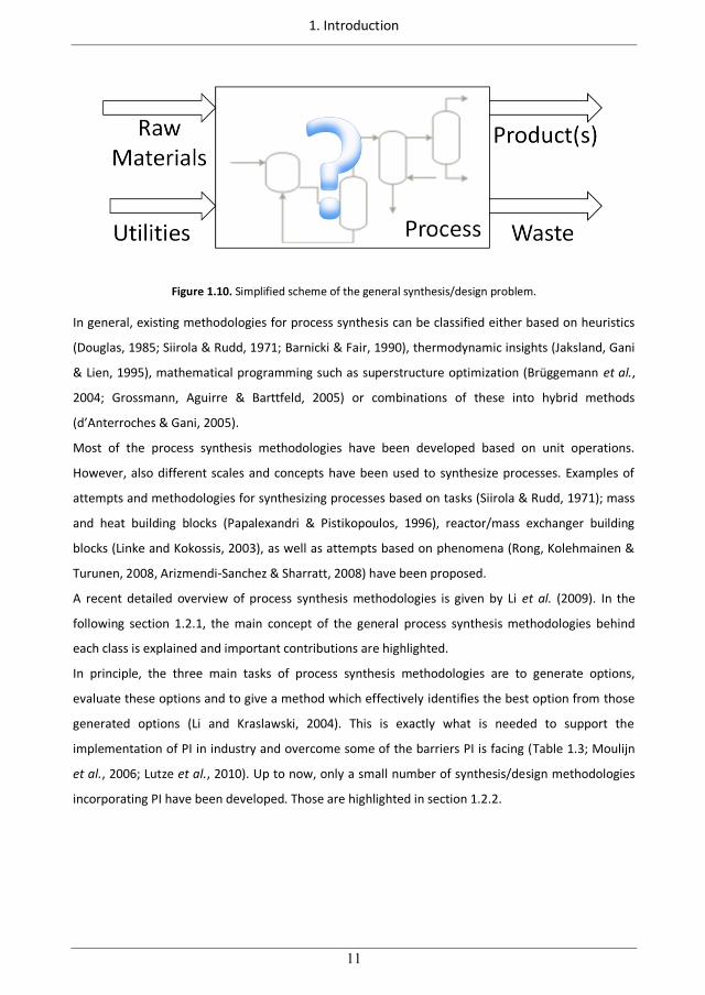
1. Introduction
11
Figure 1.10. Simplified scheme of the general synthesis/design problem.
In general, existing methodologies for process synthesis can be classified either based on heuristics
(Douglas, 1985; Siirola & Rudd, 1971; Barnicki & Fair, 1990), thermodynamic insights (Jaksland, Gani
& Lien, 1995), mathematical programming such as superstructure optimization (Brüggemann et al.,
2004; Grossmann, Aguirre & Barttfeld, 2005) or combinations of these into hybrid methods
(d’Anterroches & Gani, 2005).
Most of the process synthesis methodologies have been developed based on unit operations.
However, also different scales and concepts have been used to synthesize processes. Examples of
attempts and methodologies for synthesizing processes based on tasks (Siirola & Rudd, 1971); mass
and heat building blocks (Papalexandri & Pistikopoulos, 1996), reactor/mass exchanger building
blocks (Linke and Kokossis, 2003), as well as attempts based on phenomena (Rong, Kolehmainen &
Turunen, 2008, Arizmendi-Sanchez & Sharratt, 2008) have been proposed.
A recent detailed overview of process synthesis methodologies is given by Li et al. (2009). In the
following section 1.2.1, the main concept of the general process synthesis methodologies behind
each class is explained and important contributions are highlighted.
In principle, the three main tasks of process synthesis methodologies are to generate options,
evaluate these options and to give a method which effectively identifies the best option from those
generated options (Li and Kraslawski, 2004). This is exactly what is needed to support the
implementation of PI in industry and overcome some of the barriers PI is facing (Table 1.3; Moulijn
et al., 2006; Lutze et al., 2010). Up to now, only a small number of synthesis/design methodologies
incorporating PI have been developed. Those are highlighted in section 1.2.2.
41
1. Introduction
12
1.2.1. General process synthesis/design methodologies
Process synthesis based on heuristics:
Heuristics are a set of rules based on experience. Process synthesis based on heuristics apply
heuristics for the selection of an equipment and for identification of the position of an equipment
within the process flowsheet exploiting available process knowledge and process specifications.Two
examples for heuristic rules (Douglas, 1985) are to decide which process scenario is necessary (“Use
a continuous process for a large capacity process”) or when a separation needs to be done (“Perform
the easiest separation first”).
Examples of this class are the heuristics for separation systems mostly for processes for the chemical
industry (Siirola & Rudd, 1971; Barnicki & Fair, 1990) as well as recently for downstream processes
for bioprocesses (Bauer & Schembecker, 2008).
One of the most important synthesis tools using heuristics within this class is the hierarchical
decomposition by Douglas (1985). He decomposes the synthesis problems into 5 decision blocks:
1. Batch versus continuous.
2. Input–output structure of the flowsheet.
3. Recycle structure and reactor considerations.
4. Separation system synthesis.
5. Heat exchange network.
All of those decision blocks need to be filled with heuristic rules. Barnicki, Hoyme and Siirola (2006)
give an exhaustive list of heuristics based on experience for selection of feasible separation process
units (decision block 4.). The methodology enables the quick and stepwise evaluation of the
synthesis problem. It has been shown to be successfully applied to the hydrodealkylation of toluene
(Douglas, 1985).
However, the disadvantage of this approach is that all sub-problems are solved separately, especially
reaction and separation not allowing synergy effects between those. Another disadvantage of pure
heuristic approaches are that existing rules may be contradictory (“Perform easiest separation first”
and “Remove component with the largest amount in the stream first”) and that experience with this
equipment has to be built before being able to describe it properly into heuristics. Also, heuristics
identifying specific equipment may be contradictory.
Process synthesis based on thermodynamic insights:
Knowledge about the thermodynamic behavior of all components within the process is exploited in
process synthesis tools based on thermodynamic insights.
42
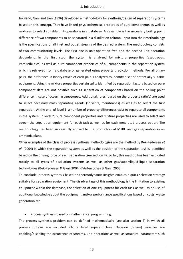
1. Introduction
13
Jaksland, Gani and Lien (1996) developed a methodology for synthesis/design of separation systems
based on this concept. They have linked physicochemical properties of pure components as well as
mixtures to select suitable unit-operations in a database. An example is the necessary boiling point
difference of two components to be separated in a distillation column. Input into their methodology
is the specifications of all inlet and outlet streams of the desired system. The methodology consists
of two communicating levels. The first one is unit-operation free and the second unit-operation
dependent. In the first step, the system is analyzed by mixture properties (azeotropes,
immiscibilities) as well as pure component properties of all components in the separation system
which is retrieved from a database or generated using property prediction methods. For all binary
pairs, the difference in binary ratio’s of each pair is analyzed to identify a set of potentially suitable
equipment. Using the mixture properties certain splits identified by separation factors based on pure
component data are not possible such as separation of components based on the boiling point
difference in case of occurring azeotropes. Additional, rules (based on the property ratio’s) are used
to select necessary mass separating agents (solvents, membranes) as well as to select the first
separation. At the end, of level 1, a number of property differences exist to separate all components
in the system. In level 2, pure component properties and mixture properties are used to select and
screen the separation equipment for each task as well as for each generated process option. The
methodology has been successfully applied to the production of MTBE and gas separation in an
ammonia plant.
Other examples of the class of process synthesis methodologies are the method by Bek-Pedersen et
al. (2004) in which the separation system as well as the position of the separation task is identified
based on the driving force of each separation (see section 4). So far, this method has been exploited
mostly to all types of distillation systems as well as other gas/vapor/liquid-liquid separation
technologies (Bek-Pedersen & Gani, 2004; d’Anterroches & Gani, 2005).
To conclude, process synthesis based on thermodynamic insights enables a quick selection strategy
suitable for separation equipment. The disadvantage of this methodology is the limitation to existing
equipment within the database, the selection of one equipment for each task as well as no use of
additional knowledge about the equipment and/or performance specifications based on costs, waste
generation etc.
Process synthesis based on mathematical programming:
The process synthesis problem can be defined mathematically (see also section 2) in which all
process options are included into a fixed superstructure. Decision (binary) variables are
enabling/disabling the occurrence of streams, unit-operations as well as structural parameters such
43
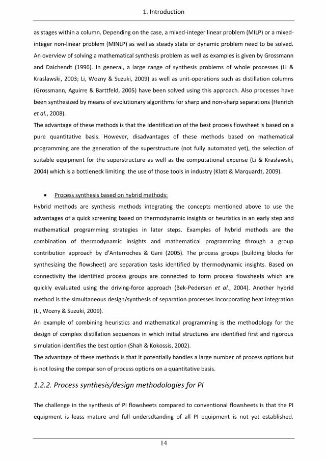
1. Introduction
14
as stages within a column. Depending on the case, a mixed-integer linear problem (MILP) or a mixed-
integer non-linear problem (MINLP) as well as steady state or dynamic problem need to be solved.
An overview of solving a mathematical synthesis problem as well as examples is given by Grossmann
and Daichendt (1996). In general, a large range of synthesis problems of whole processes (Li &
Kraslawski, 2003; Li, Wozny & Suzuki, 2009) as well as unit-operations such as distillation columns
(Grossmann, Aguirre & Barttfeld, 2005) have been solved using this approach. Also processes have
been synthesized by means of evolutionary algorithms for sharp and non-sharp separations (Henrich
et al., 2008).
The advantage of these methods is that the identification of the best process flowsheet is based on a
pure quantitative basis. However, disadvantages of these methods based on mathematical
programming are the generation of the superstructure (not fully automated yet), the selection of
suitable equipment for the superstructure as well as the computational expense (Li & Kras awski,
2004) which is a bottleneck limiting the use of those tools in industry (Klatt & Marquardt, 2009).
Process synthesis based on hybrid methods:
Hybrid methods are synthesis methods integrating the concepts mentioned above to use the
advantages of a quick screening based on thermodynamic insights or heuristics in an early step and
mathematical programming strategies in later steps. Examples of hybrid methods are the
combination of thermodynamic insights and mathematical programming through a group
contribution approach by d’Anterroches & Gani (2005). The process groups (building blocks for
synthesizing the flowsheet) are separation tasks identified by thermodynamic insights. Based on
connectivity the identified process groups are connected to form process flowsheets which are
quickly evaluated using the driving-force approach (Bek-Pedersen et al., 2004). Another hybrid
method is the simultaneous design/synthesis of separation processes incorporating heat integration
(Li, Wozny & Suzuki, 2009).
An example of combining heuristics and mathematical programming is the methodology for the
design of complex distillation sequences in which initial structures are identified first and rigorous
simulation identifies the best option (Shah & Kokossis, 2002).
The advantage of these methods is that it potentially handles a large number of process options but
is not losing the comparison of process options on a quantitative basis.
1.2.2. Process synthesis/design methodologies for PI
The challenge in the synthesis of PI flowsheets compared to conventional flowsheets is that the PI
equipment is leass mature and full undersdtanding of all PI equipment is not yet established.
44
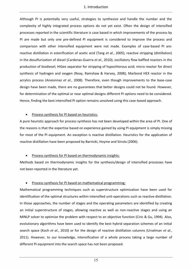
1. Introduction
15
Although PI is potentially very useful, strategies to synthesize and handle the number and the
complexity of highly integrated process options do not yet exist. Often the design of intensified
processes reported in the scientific literature is case based in which improvements of the process by
PI are made but only one pre-defined PI equipment is considered to improve the process and
comparison with other intensified equipment were not made. Examples of case-based PI are:
reactive distillation in esterification of acetic acid (Tang et al., 2005); reactive stripping (distillation)
in the desulfurization of diesel (Cardenas-Guerra et al., 2010); oscillatory flow baffled reactors in the
production of biodiesel; HiGee separator for stripping of hypochlorous acid; micro reactor for direct
synthesis of hydrogen and oxygen (Reay, Ramshaw & Harvey, 2008); Marbond HEX reactor in the
acrylics process (Anxionnaz et al., 2008). Therefore, even though improvements to the base-case
design have been made, there are no guarantees that better designs could not be found. However,
for determination of the optimal or near optimal designs different PI options need to be considered.
Hence, finding the best intensified PI option remains unsolved using this case-based approach.
Process synthesis for PI based on heuristics:
A pure heuristic approach for process synthesis has not been developed within the area of PI. One of
the reasons is that the expertise based on experience gained by using PI equipment is simply missing
for most of the PI equipment. An exception is reactive distillation. Heuristics for the application of
reactive distillation have been proposed by Barnicki, Hoyme and Siirola (2006).
Process synthesis for PI based on thermodynamic insights:
Methods based on thermodynamic insights for the synthesis/design of intensified processes have
not been reported in the literature yet.
Process synthesis for PI based on mathematical programming:
Mathematical programming techniques such as superstructure optimization have been used for
identification of the optimal structures within intensified unit-operations such as reactive distillation.
In those approaches, the number of stages and the operating parameters are identified by creating
an initial superstructure of stages, allowing reactive as well as non-reactive stages and using an
MINLP solver to optimize the problem with respect to an objective function (Ciric & Gu, 1994). Also,
evolutionary algorithms have been used to identify the best hybrid separation schemes of an initial
search space (Koch et al., 2010) or for the design of reactive distillation columns (Urselman et al.,
2011). However, to our knowledge, intensification of a whole process taking a large number of
different PI equipment into the search space has not been proposed.
45
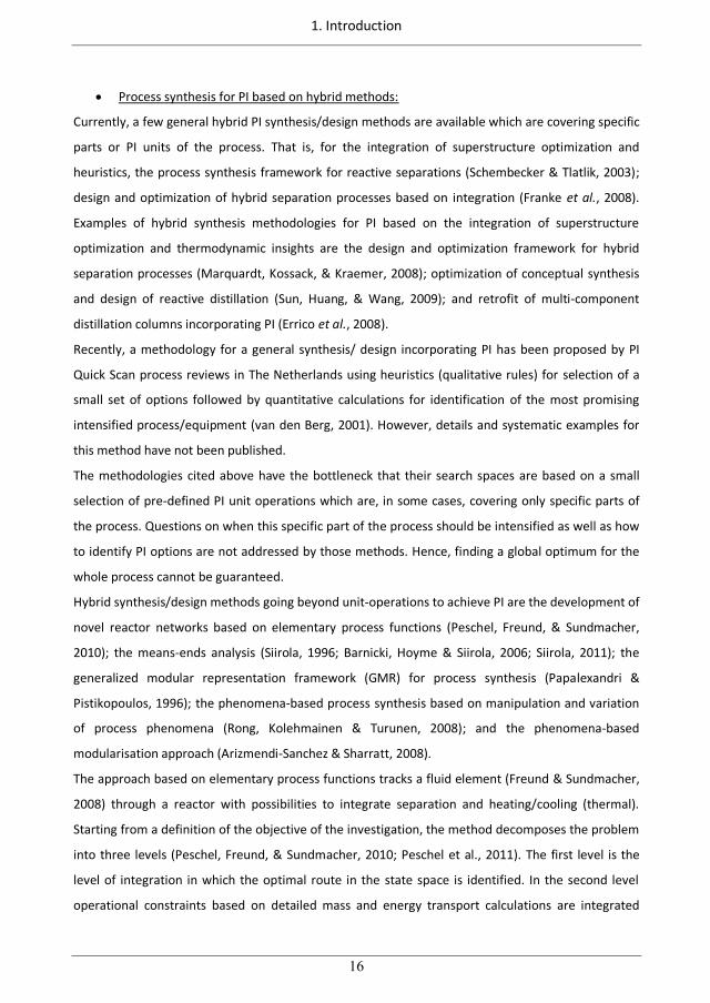
1. Introduction
16
Process synthesis for PI based on hybrid methods:
Currently, a few general hybrid PI synthesis/design methods are available which are covering specific
parts or PI units of the process. That is, for the integration of superstructure optimization and
heuristics, the process synthesis framework for reactive separations (Schembecker & Tlatlik, 2003);
design and optimization of hybrid separation processes based on integration (Franke et al., 2008).
Examples of hybrid synthesis methodologies for PI based on the integration of superstructure
optimization and thermodynamic insights are the design and optimization framework for hybrid
separation processes (Marquardt, Kossack, & Kraemer, 2008); optimization of conceptual synthesis
and design of reactive distillation (Sun, Huang, & Wang, 2009); and retrofit of multi-component
distillation columns incorporating PI (Errico et al., 2008).
Recently, a methodology for a general synthesis/ design incorporating PI has been proposed by PI
Quick Scan process reviews in The Netherlands using heuristics (qualitative rules) for selection of a
small set of options followed by quantitative calculations for identification of the most promising
intensified process/equipment (van den Berg, 2001). However, details and systematic examples for
this method have not been published.
The methodologies cited above have the bottleneck that their search spaces are based on a small
selection of pre-defined PI unit operations which are, in some cases, covering only specific parts of
the process. Questions on when this specific part of the process should be intensified as well as how
to identify PI options are not addressed by those methods. Hence, finding a global optimum for the
whole process cannot be guaranteed.
Hybrid synthesis/design methods going beyond unit-operations to achieve PI are the development of
novel reactor networks based on elementary process functions (Peschel, Freund, & Sundmacher,
2010); the means-ends analysis (Siirola, 1996; Barnicki, Hoyme & Siirola, 2006; Siirola, 2011); the
generalized modular representation framework (GMR) for process synthesis (Papalexandri &
Pistikopoulos, 1996); the phenomena-based process synthesis based on manipulation and variation
of process phenomena (Rong, Kolehmainen & Turunen, 2008); and the phenomena-based
modularisation approach (Arizmendi-Sanchez & Sharratt, 2008).
The approach based on elementary process functions tracks a fluid element (Freund & Sundmacher,
2008) through a reactor with possibilities to integrate separation and heating/cooling (thermal).
Starting from a definition of the objective of the investigation, the method decomposes the problem
into three levels (Peschel, Freund, & Sundmacher, 2010; Peschel et al., 2011). The first level is the
level of integration in which the optimal route in the state space is identified. In the second level
operational constraints based on detailed mass and energy transport calculations are integrated
46
1. Introduction
17
within the design of level 1. In the last level, the unit operation is identified to screen for technical
constraints of the design. Reactor parameters such as interfacial areas, residence time and number
of units, are not defined a priori but are investigated through a stepwise procedure. The method has
been illustrated for a SO2 oxidation reactor and a hydrofurmylation biphasic reactor. The knowledge-
base or rules necessary to identify the unit-operations and the functions from the analysis has not
been presented.
In the means-ends analysis approach by Siirola et al. (1996, 2006, 2011), the process inlet and outlet
specifications are defined. Based on a set of rules, the tasks to satisfy the specifications are
identified. By variations based on heuristics (expert knowledge) different process options are
generated which are evaluated based on sets of performance criteria. The method has been
illustrated by the generation of the reactive distillation unit for the production of methyl-acetate.
The detailed step-by-step procedure for this case study is given in the appendix A.5. However, even
though novel process/units may be identified, the application is not simple. Rules and/or algorithms
for identification and variations of tasks as well as for identification of unit operations have not been
published. Furthermore, it does not aim to generate all potentially feasible options and based on this
cannot guarantee to find a (global) optimal solution.
Process synthesis by the GMR-approach is based on heat and mass building blocks instead of defined
(conventional) equipment. Heat and mass building blocks may be or may not be connected using a
set of connectivity rules. If a given connection of these blocks gives a feasible and promising
solution, then in a subsequent step, unit operation(s) are identified for those. Until now, this
approach has been successfully illustrated for column synthesis/design such as distillation, reactive
distillation and absorption (Papalexandri & Pistikopoulos, 1996; Algusane et al., 2003). The selection
of the initial search space of building blocks is based on heuristics and thermodynamic insights. A
complete set of rules how to identify unit operations has not been given yet. Even though it is a very
promising approach, since then (2003), no additional papers have been published using this
methodology.
The synthesis concept by Rong et al. (2004, 2008) is based on process phenomena. They classified
process phenomena into “chemistry and chemical reaction phenomena, materials phases and
transport phenomena, phases behavior and separation phenomena etc.”. Process phenomena are
characterized by surface materials, operation modes, flow pattern, facility medium, geometry,
energy sources, key variables as well as components and phases. Their methodology decomposes
the synthesis problem into 10 hierarchical steps. The heart of their method consists of trial-and-error
variations of the characteristics for the identified key process phenomena through seven different
suggested PI principles. The method has been briefly illustrated by two conceptual examples which
47
1. Introduction
18
are the production of peracetic acid (Rong, Kolehmainen & Turunen, 2008) and hydrogen peroxide
(Rong et al., 2004). Details about algorithms and the stepwise procedure are not given, including: a
definition/description and systematic identification of phenomena; as well as strategies for
variations of these phenomena; techniques how to find all currently available options; and a solution
approach how to identify the best option. For each of their conceptual examples only the final
design of the intensified process is presented.
Another concept, using phenomena to synthesize potentially novel process solutions is the
modularisation approach by Arizmendi-Sanchez and Sharratt (2008). They have classified
phenomena into phenomena in the structural level for the description of phases and interfaces; and
phenomena in the behavioral level for the description of mass transfer, phase change, energy,
change conditions and mechanical operations. Their concept is to aggregate phenomena to form
phases. Phases can be aggregated to form tasks (such as stages or devices). Tasks can be aggregated
to represent the whole process. Until now, only the library and classification of phenomena as well
as the representation of one unit by phenomena have been presented. No details on algorithms,
necessary tools and solution techniques to synthesize processes based on their modularisation
approach have been published.
Hence, even though promising attempts in synthesis/design to achieve PI have been proposed,
systematically finding the best intensified PI option for a whole process remains unsolved using the
approaches above. This counts for the unit-operation based concepts as well as for the concepts
going beyond unit-operations.
1.3. Motivation and objectives for this PhD-project
PI has lead to the development of a significant number of new equipment concepts and operating
strategies to improve processes with respect to a range of different objectives (see section 1.1).
Despite the potential, only a small number of successful implementations of PI equipment have been
reported (Harmsen, 2010) and there are a number of challenges with respect to its application
(Table 1.3). The application of process synthesis can overcome these issues (Moulijn et al., 2006).
Currently available process synthesis/design methods incorporating PI are limited to specific parts or
units of the process (see section 1.2). It is believed, however, that PI has the biggest impact on
performance improvement when applied to the whole process (Moulijn et al., 2006). Therefore,
even though improvements to the base-case design have been made, there are no guarantees that
better designs could not be found. This has not been tackled in the current methodologies which are
not focusing to intensify the whole process on a quantitative basis.
Another gap is how to design/synthesize PI going beyond PI equipment currently in existence which
48
1. Introduction
19
may achieve potentially even higher improvements in the process (Freund & Sundmacher, 2008).
Until now, some promising concepts to generate potentially novel PI designs have been proposed in
literature but have not been developed in full detail giving algorithms for a systematic approach so
far (see section 1.2).
Therefore, to push the implementation of process intensification, the following main objective of
this PhD-project is the:
Development of a systematic synthesis/design methodology to achieve process intensification.
This methodology should generate PI options improving a target specification, evaluate these PI
options for feasibility and identifies the best options from the remaining options on a quantitative
basis. Therefore, this methodology should be able to handle a large number of options. The method
of solution should be efficient, robust and reliable. There should be workflows which guide the user
through all decisions/actions to be made and integrates the methodology to all tools, databases,
models which are necessary to take decisions. The methodology should be able to generate PI
options using existing PI equipment for fast retrofit of an existing process. It should also be able to
generate novel solutions going beyond PI equipment currently existing. For this the fundamental
definition of PI (see section 1.1.1) should be exploited to enhance process phenomena using the PI
principles (a-d). The methodology should contain a well-defined procedure for screening using a
well-defined list of performance criteria from which the screening of PI options is based. The
methodology should be generic, meaning that all tools, workflows and models are applicable for a
wide range of different process industries.
1.4. Structure of the thesis
In chapter 2, the theoretical background for the developed methodology is explained in detail. That
includes the decomposition-based solution approach used for handling the large number of process
options as well as the developed concept to generate novel PI solutions by using a phenomena
based approach for PI flowsheet design. In chapter 3, the developed workflow of the methodology is
presented in detail including all algorithms and sub-algorithms. In chapter 4, the supporting tools
and methods which have been developed and/or applied in order to follow the workflow are
described. In chapter 5, the application of the unit-operation based synthesis/design methodology is
highlighted by case studies. In chapter 6, case studies highlighting the application of the
phenomena-based synthesis/design methodology are presented. The developed synthesis/design
methodology and the results of their application to the case studies are discussed in chapter 7. That
gives the basis for a summary of the main achievements of this PhD-project and for an outlook for
future work in chapter 8.
49

1. Introduction
20
50
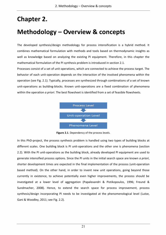
2. Methodology – Overview & concepts
21
Chapter 2.
Methodology – Overview & concepts
The developed synthesis/design methodology for process intensification is a hybrid method. It
combines mathematical formulation with methods and tools based on thermodynamic insights as
well as knowledge based on analyzing the existing PI equipment. Therefore, in this chapter the
mathematical formulation of the PI synthesis problem is introduced in section 2.1.
Processes consist of a set of unit operations, which are connected to achieve the process target. The
behavior of each unit-operation depends on the interaction of the involved phenomena within the
operation (see Fig. 2.1). Typically, processes are synthesized through combinations of a set of known
unit-operations as building-blocks. Known unit-operations are a fixed combination of phenomena
within the operation a priori. The best flowsheet is identified from a set of feasible flowsheets.
Figure 2.1. Dependency of the process levels.
In this PhD-project, the process synthesis problem is handled using two types of building blocks at
different scales. One building block is PI unit-operations and the other one is phenomena (section
2.2). With the PI unit-operations as the building block, already developed PI equipment are used to
generate intensified process options. Since the PI units in the initial search space are known a priori,
shorter development times are expected in the final implementation of the process (unit-operation
based method). On the other hand, in order to invent new unit operations, going beyond those
currently in existence, to achieve potentially even higher improvements, the process should be
investigated at a lower level of aggregation (Papalexandri & Pistikopoulos, 1996; Freund &
Sundmacher, 2008). Hence, to extend the search space for process improvement, process
synthesis/design incorporating PI needs to be investigated at the phenomenological level (Lutze,
Gani & Woodley, 2011; see Fig. 2.2).
51
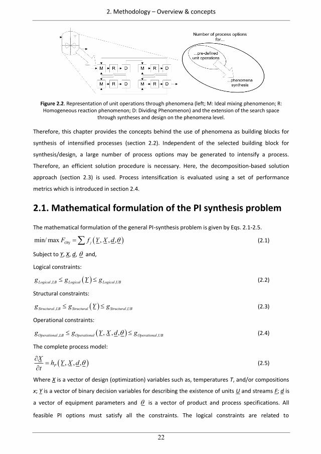
2. Methodology – Overview & concepts
22
Figure 2.2. Representation of unit operations through phenomena (left; M: Ideal mixing phenomenon; R:
Homogeneous reaction phenomenon; D: Dividing Phenomenon) and the extension of the search space through syntheses and design on the phenomena level.
Therefore, this chapter provides the concepts behind the use of phenomena as building blocks for
synthesis of intensified processes (section 2.2). Independent of the selected building block for
synthesis/design, a large number of process options may be generated to intensify a process.
Therefore, an efficient solution procedure is necessary. Here, the decomposition-based solution
approach (section 2.3) is used. Process intensification is evaluated using a set of performance
metrics which is introduced in section 2.4.
2.1. Mathematical formulation of the PI synthesis problem
The mathematical formulation of the general PI-synthesis problem is given by Eqs. 2.1-2.5.
min/ max , , ,Obj jF f Y X d (2.1)
Subject to Y, X, d, and,
Logical constraints:
, ,Logical LB Logical Logical UBg g Y g (2.2)
Structural constraints:
, ,Structural LB Structural Structural UBg g Y g (2.3)
Operational constraints:
, ,, , ,Operational LB Operational Operational UBg g Y X d g (2.4)
The complete process model:
, , ,PX h Y X dt
(2.5)
Where X is a vector of design (optimization) variables such as, temperatures T, and/or compositions
x; Y is a vector of binary decision variables for describing the existence of units U and streams F; d is
a vector of equipment parameters and is a vector of product and process specifications. All
feasible PI options must satisfy all the constraints. The logical constraints are related to
52
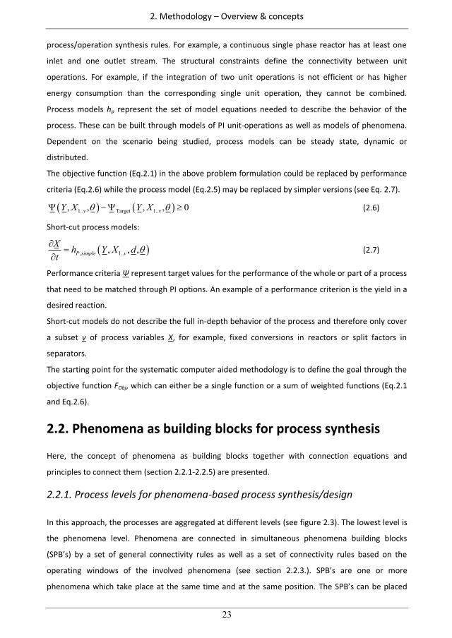
2. Methodology – Overview & concepts
23
process/operation synthesis rules. For example, a continuous single phase reactor has at least one
inlet and one outlet stream. The structural constraints define the connectivity between unit
operations. For example, if the integration of two unit operations is not efficient or has higher
energy consumption than the corresponding single unit operation, they cannot be combined.
Process models hp represent the set of model equations needed to describe the behavior of the
process. These can be built through models of PI unit-operations as well as models of phenomena.
Dependent on the scenario being studied, process models can be steady state, dynamic or
distributed.
The objective function (Eq.2.1) in the above problem formulation could be replaced by performance
criteria (Eq.2.6) while the process model (Eq.2.5) may be replaced by simpler versions (see Eq. 2.7).
1.. Target 1.., , , , 0v vY X Y X (2.6)
Short-cut process models:
, 1.., , ,P simple vX h Y X dt
(2.7)
Performance criteria represent target values for the performance of the whole or part of a process
that need to be matched through PI options. An example of a performance criterion is the yield in a
desired reaction.
Short-cut models do not describe the full in-depth behavior of the process and therefore only cover
a subset v of process variables X, for example, fixed conversions in reactors or split factors in
separators.
The starting point for the systematic computer aided methodology is to define the goal through the
objective function FObj, which can either be a single function or a sum of weighted functions (Eq.2.1
and Eq.2.6).
2.2. Phenomena as building blocks for process synthesis
Here, the concept of phenomena as building blocks together with connection equations and
principles to connect them (section 2.2.1-2.2.5) are presented.
2.2.1. Process levels for phenomena-based process synthesis/design
In this approach, the processes are aggregated at different levels (see figure 2.3). The lowest level is
the phenomena level. Phenomena are connected in simultaneous phenomena building blocks
(SPB’s) by a set of general connectivity rules as well as a set of connectivity rules based on the
operating windows of the involved phenomena (see section 2.2.3.). SPB’s are one or more
phenomena which take place at the same time and at the same position. The SPB’s can be placed
53
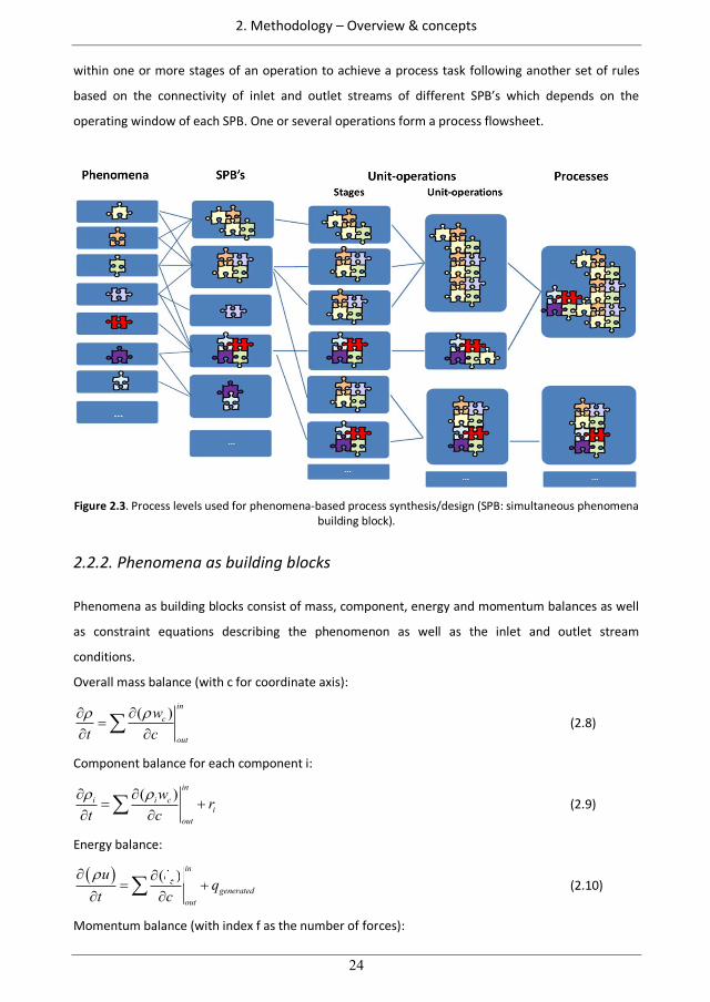
2. Methodology – Overview & concepts
24
within one or more stages of an operation to achieve a process task following another set of rules
based on the connectivity of inlet and outlet streams of different SPB’s which depends on the
operating window of each SPB. One or several operations form a process flowsheet.
Figure 2.3. Process levels used for phenomena-based process synthesis/design (SPB: simultaneous phenomena
building block).
2.2.2. Phenomena as building blocks
Phenomena as building blocks consist of mass, component, energy and momentum balances as well
as constraint equations describing the phenomenon as well as the inlet and outlet stream
conditions.
Overall mass balance (with c for coordinate axis):
( ) inc
out
wt c
(2.8)
Component balance for each component i:
( ) ini i c
iout
w rt c
(2.9)
Energy balance:
( ) inc
generatedout
u e qt c
) in) (2.10)
Momentum balance (with index f as the number of forces):
54
2. Methodology – Overview & concepts
25
ff
wf
t (2.11)
All equations in the building blocks have to be linked to additional constitutive equations such as
equations representing thermodynamic properties or reaction kinetics.
In general, phenomena can be classified into 8 different classes:
Mixing: Mixing phenomena describe the mixing within one phase or between several
existing phases.
Stream dividing: A stream dividing phenomenon divides a stream into two or more streams.
Temperature, pressure and concentrations remain unchanged.
Phase contact: Phase contact phenomena describe the contact (and the resistances) directly
at the phase boundary of two (or more) phases.
Phase transition: These phenomena describe the mass transfer of components between at
least two phases. An example of a phase transition phenomenon is the vapor-liquid
equilibrium relationship.
Phase change: These phenomena describe the change of state of a complete stream.
Concentrations within the phase do not change. An example is full evaporation of a liquid
stream.
Phase separation: Phase separation phenomena describe the degree of separation of the
two phases. This may be ideal, meaning that the outlet streams are pure with respect to the
occurring phases within each outlet stream or not.
Reaction: Within a reaction phenomenon the mass of one (or more than one) component is
changed between inlet and outlet streams.
Energy transfer phenomena: Energy supply/removal between energy sources and sinks are
described with energy transfer phenomena
Each class of phenomena (except of the stream dividing) can be further sub-classified. For example,
for phase transition phenomena the subclasses are depending on the involved phases (e.g. V-L, L-L).
For each class of phenomena the number of inlet and outlet streams are defined which is important
for connectivity between phenomena of different classes. Mixing phenomena have minimum one
inlet stream and one outlet stream while dividing phenomena have one inlet and minimum two
outlet streams. Reaction blocks are defined to have one inlet and one outlet stream. The inlet of
phase transition phenomena is a mixture of two phases between which the mass transfer of
components is realized. The outlet of a phase transition phenomenon is a mixture of two phases.
Phase separation phenomena have one inlet and the number of outlets is given by the number of
55
2. Methodology – Overview & concepts
26
phases separated from each other within this phenomenon. Energy transfer phenomena such as
heating/ cooling and pressurizing/expanding are defined to have either one inlet and one outlet or
two inlet and two outlet streams, where the streams are not in contact. An overview over the
number of inlet and out streams for different phenomena is presented in Table 2.1. An overview of
the states of these inlet/outlet streams of some phenomena is presented in Table 2.2.
Currently, 53 phenomena are available in the phenomena library and the list is given in appendix
A.2.
56
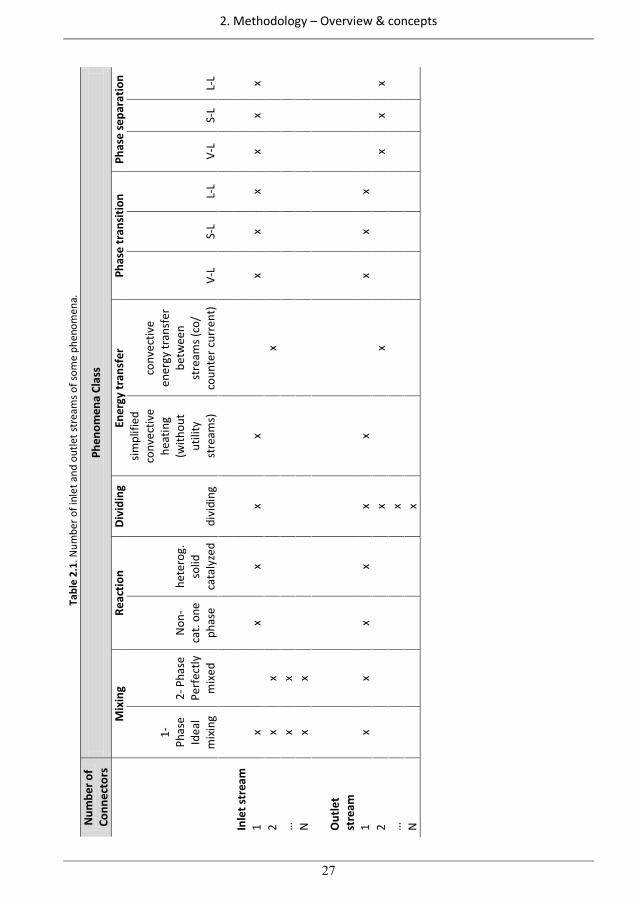
2. Methodology – Overview & concepts
27
Tabl
e 2.
1. N
umbe
r of i
nlet
and
out
let s
trea
ms o
f som
e ph
enom
ena.
N
umbe
r of
Conn
ecto
rs
Phen
omen
a Cl
ass
M
ixin
g Re
actio
n Di
vidi
ng
Ener
gy tr
ansf
er
Phas
e tr
ansit
ion
Phas
e se
para
tion
1-
Phas
e Id
eal
mix
ing
2- P
hase
Pe
rfec
tly
mix
ed
Non
-ca
t. on
e ph
ase
hete
rog.
so
lid
cata
lyze
d di
vidi
ng
simpl
ified
co
nvec
tive
heat
ing
(with
out
utili
ty
stre
ams)
conv
ectiv
e en
ergy
tran
sfer
be
twee
n st
ream
s (co
/ co
unte
r cur
rent
) V-
L S-
L L-
L V-
L S-
L L-
L
In
let s
trea
m
1
x
x x
x x
x
x x
x x
x 2
x x
x
…
x
x
N
x x
O
utle
t st
ream
1 x
x x
x x
x
x x
x
2
x
x
x
x x
…
x
N
x
57
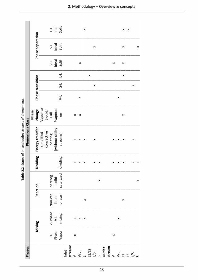
2. Methodology – Overview & concepts
28
Tabl
e 2.
2. S
tate
s of i
n- a
nd o
utle
t str
eam
s of p
heno
men
a.
Phas
es
Phen
omen
a Cl
ass
M
ixin
g Re
actio
n Di
vidi
ng
Ener
gy tr
ansf
er
Phas
e ch
ange
Ph
ase
tran
sitio
n Ph
ase
sepa
ratio
n
1-
Phas
e Va
por
2- P
hase
V-
L m
ixin
g
Non
-cat
. liq
uid
phas
e
hete
rog.
so
lid
cata
lyze
d di
vidi
ng
simpl
ified
co
nvec
tive
heat
ing
(with
out u
tility
st
ream
s)
Vapo
r to
Liqu
id:
Full
Evap
orat
ion
V-
L S-
L L-
L
V-L
Idea
l Sp
lit
S-L
Idea
l Sp
lit
L-L
Idea
l Sp
lit
Inle
t st
ream
:
V x
x
x
x x
V/L
x
x x
x x
x
L
x
x
x x
x L1
/L2
x
L/
S
x
x
x
x
S
x x
Out
let
stre
am
V x
x
x
x
V/L
x
x x
x
L1
x
x
x x
x x
x x
L2
x L/
S
x
x
x
S
x x
x
58
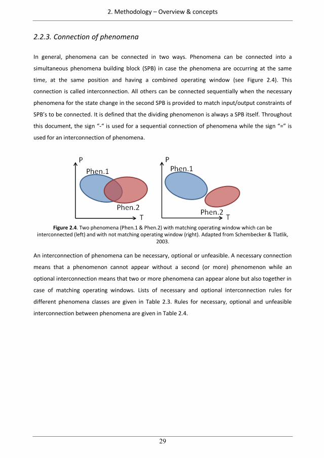
2. Methodology – Overview & concepts
29
2.2.3. Connection of phenomena
In general, phenomena can be connected in two ways. Phenomena can be connected into a
simultaneous phenomena building block (SPB) in case the phenomena are occurring at the same
time, at the same position and having a combined operating window (see Figure 2.4). This
connection is called interconnection. All others can be connected sequentially when the necessary
phenomena for the state change in the second SPB is provided to match input/output constraints of
SPB’s to be connected. It is defined that the dividing phenomenon is always a SPB itself. Throughout
this document, the sign “-“ is used for a sequential connection of phenomena while the sign “=” is
used for an interconnection of phenomena.
Figure 2.4. Two phenomena (Phen.1 & Phen.2) with matching operating window which can be
interconnected (left) and with not matching operating window (right). Adapted from Schembecker & Tlatlik, 2003.
An interconnection of phenomena can be necessary, optional or unfeasible. A necessary connection
means that a phenomenon cannot appear without a second (or more) phenomenon while an
optional interconnection means that two or more phenomena can appear alone but also together in
case of matching operating windows. Lists of necessary and optional interconnection rules for
different phenomena classes are given in Table 2.3. Rules for necessary, optional and unfeasible
interconnection between phenomena are given in Table 2.4.
59
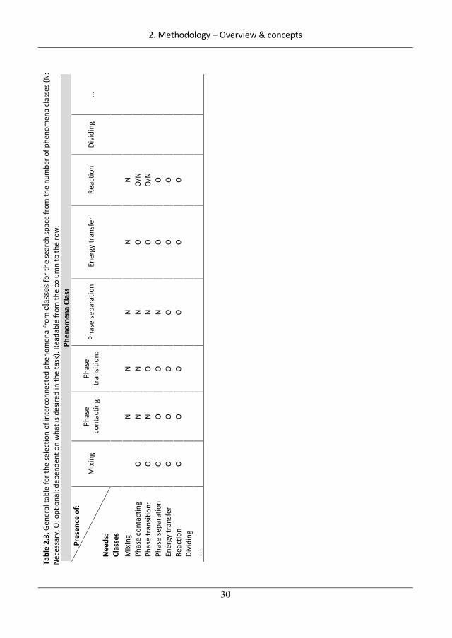
2. Methodology – Overview & concepts
30
Tabl
e 2.
3. G
ener
al ta
ble
for t
he se
lect
ion
of in
terc
onne
cted
phe
nom
ena
from
clas
ses f
or th
e se
arch
spac
e fr
om th
e nu
mbe
r of p
heno
men
a cl
asse
s (N
: N
eces
sary
, O: o
ptio
nal:
depe
nden
t on
wha
t is d
esire
d in
the
task
). Re
adab
le fr
om th
e co
lum
n to
the
row
. Ph
enom
ena
Clas
s
Pr
esen
ce o
f: N
eeds
:
Mix
ing
Phas
e co
ntac
ting
Phas
e tr
ansit
ion:
Ph
ase
sepa
ratio
n En
ergy
tran
sfer
Re
actio
n Di
vidi
ng
…
Clas
ses
Mix
ing
N
N
N
N
N
Ph
ase
cont
actin
g O
N
N
N
O
O
/N
Phas
e tr
ansit
ion:
O
N
O
N
O
O
/N
Phas
e se
para
tion
O
O
O
N
O
O
Ener
gy tr
ansf
er
O
O
O
O
O
O
Reac
tion
O
O
O
O
O
O
Divi
ding
…
60
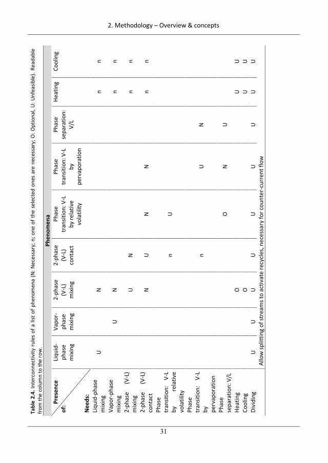
2. Methodology – Overview & concepts
31
Tabl
e 2.
4. In
terc
onne
ctiv
ity r
ules
of a
list
of p
heno
men
a (N
: Nec
essa
ry; n
; one
of t
he s
elec
ted
ones
are
nec
essa
ry; O
: Opt
iona
l, U
: Unf
easib
le).
Read
able
fr
om th
e co
lum
n to
the
row
. Ph
enom
ena
Pres
ence
of
: N
eeds
:
Liqu
id-
phas
e m
ixin
g
Vapo
r-ph
ase
mix
ing
2-ph
ase
(V-L
) m
ixin
g
2-ph
ase
(V-L
) co
ntac
t
Phas
e tr
ansit
ion:
V-L
by
rela
tive
vola
tility
Phas
e tr
ansit
ion:
V-L
by
pe
rvap
orat
ion
Phas
e se
para
tion:
V/
L
Heat
ing
Cool
ing
Liqu
id-p
hase
m
ixin
g U
N
n
n
Vapo
r-ph
ase
mix
ing
U
N
n n
2-ph
ase
(V-L
) m
ixin
g
U
N
n
n
2-ph
ase
(V-L
) co
ntac
t
N
U
N
N
n
n
Phas
e tr
ansit
ion:
V-
L by
re
lativ
e vo
latil
ity
n
U
Phas
e tr
ansit
ion:
V-
L by
pe
rvap
orat
ion
n
U
N
Phas
e se
para
tion:
V/L
O
N
U
Heat
ing
O
U U
Cool
ing
O
U U
Divi
ding
U
U U
U U
U U
U U
Allo
w sp
littin
g of
stre
ams t
o ac
tivat
e re
cycl
es, n
eces
sary
for c
ount
er-c
urre
nt fl
ow
61
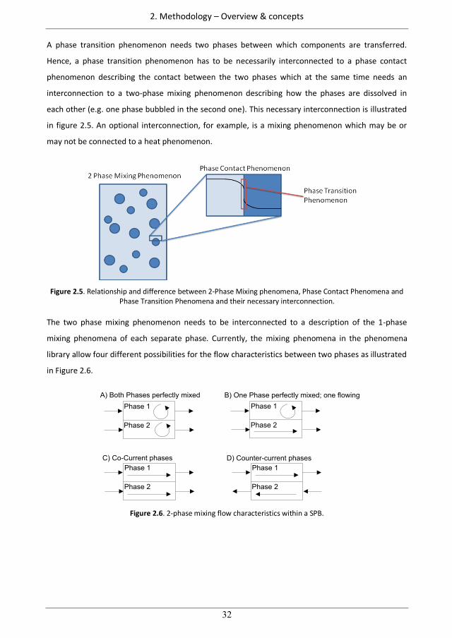
2. Methodology – Overview & concepts
32
A phase transition phenomenon needs two phases between which components are transferred.
Hence, a phase transition phenomenon has to be necessarily interconnected to a phase contact
phenomenon describing the contact between the two phases which at the same time needs an
interconnection to a two-phase mixing phenomenon describing how the phases are dissolved in
each other (e.g. one phase bubbled in the second one). This necessary interconnection is illustrated
in figure 2.5. An optional interconnection, for example, is a mixing phenomenon which may be or
may not be connected to a heat phenomenon.
Figure 2.5. Relationship and difference between 2-Phase Mixing phenomena, Phase Contact Phenomena and
Phase Transition Phenomena and their necessary interconnection. The two phase mixing phenomenon needs to be interconnected to a description of the 1-phase
mixing phenomena of each separate phase. Currently, the mixing phenomena in the phenomena
library allow four different possibilities for the flow characteristics between two phases as illustrated
in Figure 2.6.
Phase 1
Phase 2
Phase 1
Phase 2
Phase 1
Phase 2
Phase 1
Phase 2
A) Both Phases perfectly mixed B) One Phase perfectly mixed; one flowing
C) Co-Current phases D) Counter-current phases
Figure 2.6. 2-phase mixing flow characteristics within a SPB.
62
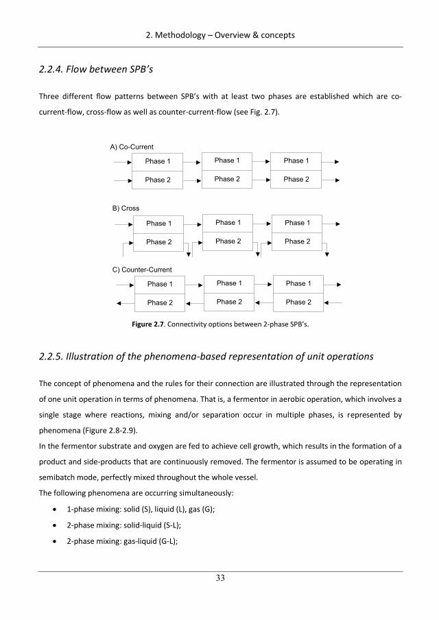
2. Methodology – Overview & concepts
33
2.2.4. Flow between SPB’s
Three different flow patterns between SPB’s with at least two phases are established which are co-
current-flow, cross-flow as well as counter-current-flow (see Fig. 2.7).
Phase 1
Phase 2
A) Co-Current
B) Cross
Phase 1
Phase 2
Phase 1
Phase 2
Phase 1
Phase 2
Phase 1
Phase 2
Phase 1
Phase 2
Phase 1
Phase 2
C) Counter-Current
Phase 1
Phase 2
Phase 1
Phase 2
Figure 2.7. Connectivity options between 2-phase SPB’s.
2.2.5. Illustration of the phenomena-based representation of unit operations
The concept of phenomena and the rules for their connection are illustrated through the representation
of one unit operation in terms of phenomena. That is, a fermentor in aerobic operation, which involves a
single stage where reactions, mixing and/or separation occur in multiple phases, is represented by
phenomena (Figure 2.8-2.9).
In the fermentor substrate and oxygen are fed to achieve cell growth, which results in the formation of a
product and side-products that are continuously removed. The fermentor is assumed to be operating in
semibatch mode, perfectly mixed throughout the whole vessel.
The following phenomena are occurring simultaneously:
1-phase mixing: solid (S), liquid (L), gas (G);
2-phase mixing: solid-liquid (S-L);
2-phase mixing: gas-liquid (G-L);
63
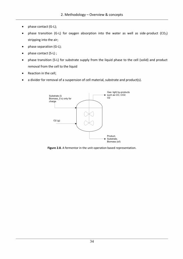
2. Methodology – Overview & concepts
34
phase contact (G-L);
phase transition (G-L) for oxygen absorption into the water as well as side-product (CO2)
stripping into the air;
phase separation (G-L);
phase contact (S-L) ;
phase transition (S-L) for substrate supply from the liquid phase to the cell (solid) and product
removal from the cell to the liquid
Reaction in the cell;
a divider for removal of a suspension of cell material, substrate and product(s).
O2 (g)
Biomass_0 s) only forcharge
Product,Substrate,Biomass (s/l)
Gas: light by-productssuch as CO, CO2;O2
Substrate (l)
Figure 2.8. A fermentor in the unit-operation based representation.
64
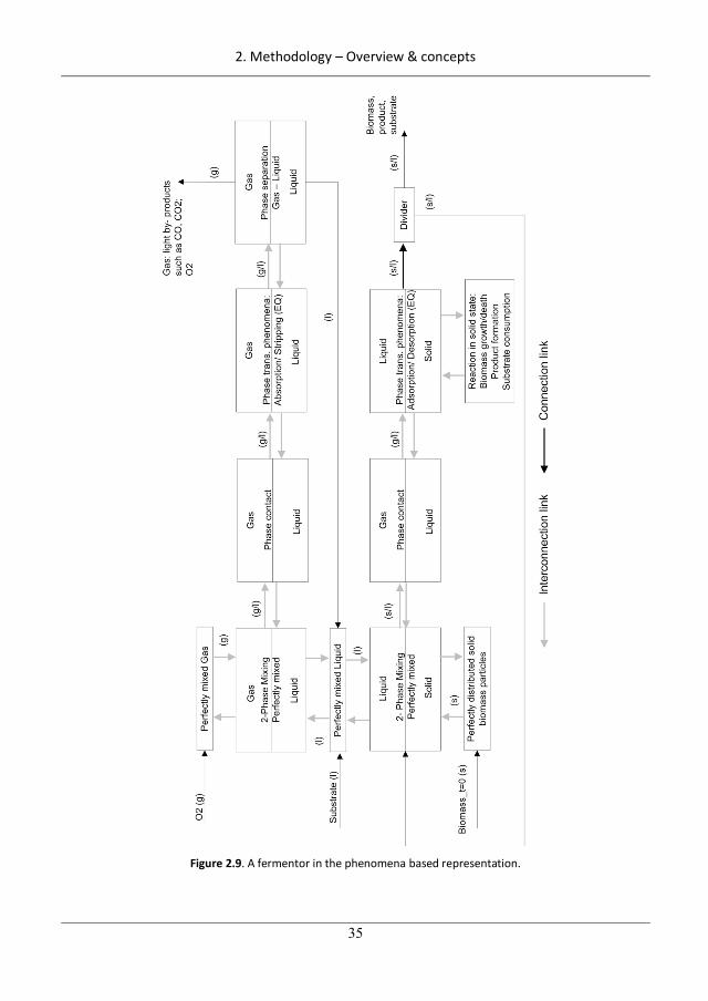
2. Methodology – Overview & concepts
35
Figure 2.9. A fermentor in the phenomena based representation.
65
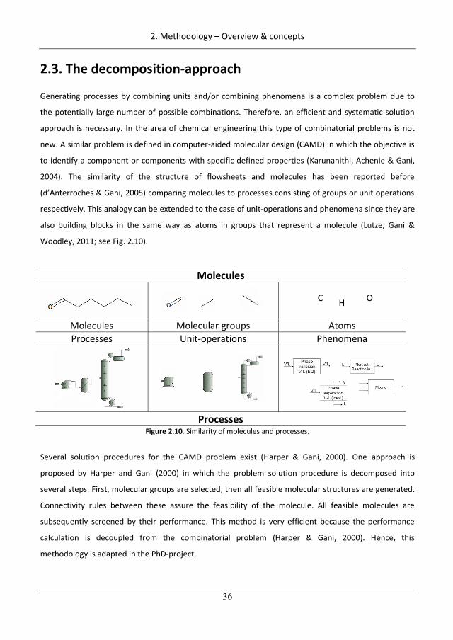
2. Methodology – Overview & concepts
36
2.3. The decomposition-approach
Generating processes by combining units and/or combining phenomena is a complex problem due to
the potentially large number of possible combinations. Therefore, an efficient and systematic solution
approach is necessary. In the area of chemical engineering this type of combinatorial problems is not
new. A similar problem is defined in computer-aided molecular design (CAMD) in which the objective is
to identify a component or components with specific defined properties (Karunanithi, Achenie & Gani,
2004). The similarity of the structure of flowsheets and molecules has been reported before
(d’Anterroches & Gani, 2005) comparing molecules to processes consisting of groups or unit operations
respectively. This analogy can be extended to the case of unit-operations and phenomena since they are
also building blocks in the same way as atoms in groups that represent a molecule (Lutze, Gani &
Woodley, 2011; see Fig. 2.10).
Molecules
C H O
Molecules Molecular groups Atoms Processes Unit-operations Phenomena
Processes Figure 2.10. Similarity of molecules and processes.
Several solution procedures for the CAMD problem exist (Harper & Gani, 2000). One approach is
proposed by Harper and Gani (2000) in which the problem solution procedure is decomposed into
several steps. First, molecular groups are selected, then all feasible molecular structures are generated.
Connectivity rules between these assure the feasibility of the molecule. All feasible molecules are
subsequently screened by their performance. This method is very efficient because the performance
calculation is decoupled from the combinatorial problem (Harper & Gani, 2000). Hence, this
methodology is adapted in the PhD-project.
66
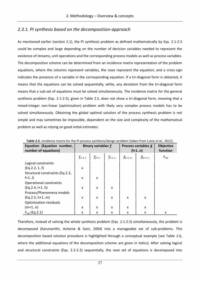
2. Methodology – Overview & concepts
37
2.3.1. PI synthesis based on the decomposition-approach
As mentioned earlier (section 2.1), the PI synthesis problem as defined mathematically by Eqs. 2.1-2.5
could be complex and large depending on the number of decision variables needed to represent the
existence of streams, unit operations and the corresponding process models as well as process variables.
The decomposition scheme can be determined from an incidence matrix representation of the problem
equations, where the columns represent variables, the rows represent the equation; and a cross-sign
indicates the presence of a variable in the corresponding equation. If a tri-diagonal form is obtained, it
means that the equations can be solved sequentially, while, any deviation from the tri-diagonal form
means that a sub-set of equations must be solved simultaneously. The incidence matrix for the general
synthesis problem (Eqs. 2.1-2.5), given in Table 2.5, does not show a tri-diagonal form, meaning that a
mixed-integer non-linear (optimization) problem with likely very complex process models has to be
solved simultaneously. Obtaining the global optimal solution of the process synthesis problem is not
simple and may sometimes be impossible, dependent on the size and complexity of the mathematical
problem as well as relying on good initial estimates.
Table 2.5. Incidence matrix for the PI process synthesis/design problem (taken from Lutze et al., 2012). Equation (Equation number, number of equations)
Binary variables Y Process variables X (l+1..n)
Objective function
Y1+1..f Yf+1..l Yl+1..o Xv+1..w Xw+1..n Fobj
Logical constraints (Eq.2.2, 1..f) x Structural constraints (Eq.2.3, f+1..l) x x Operational constraints (Eq.2.4, l+1..h) x x x Process/Phenomena models (Eq.2.5, h+1..m) x x x x x Optimization residuals (m+1..n) x x x x x Fobj (Eq.2.1) x x x x x x
Therefore, instead of solving the whole synthesis problem (Eqs. 2.1-2.5) simultaneously, the problem is
decomposed (Karunanithi, Achenie & Gani, 2004) into a manageable set of sub-problems. This
decomposition based solution procedure is highlighted through a conceptual example (see Table 2.6,
where the additional equations of the decomposition scheme are given in italics). After solving logical
and structural constraints (Eqs. 2.2-2.3) sequentially, the next set of equations is decomposed into
67
2. Methodology – Overview & concepts
38
subsets of fixed binary variables. For each of them (meaning for each existing process option),
operational constraints (Eq. 2.4) and a short-cut (simple) process/phenomena model (Eq. 2.7) are
solved. The resulting feasible set is ranked according to performance criteria (Eq. 2.6). In case all process
variables (if v=n) are fixed at this point, the objective function (Eq. 2.1) is calculated. If necessary, a small
number of the top-ranked feasible alternatives could be further optimized (solving Eqs. 2.1, 2.4-2.5) to
determine the optimal solution. Here, rigorous models are used (Eq. 2.5).
68
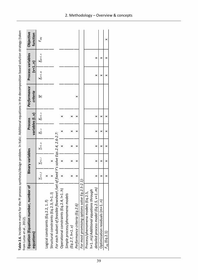
2. Methodology – Overview & concepts
39
Tabl
e 2.
6. In
ciden
ce m
atrix
for t
he P
I pro
cess
synt
hesis
/des
ign
prob
lem
. In
Italic
: Add
ition
al e
quat
ions
in th
e de
com
posit
ion
base
d so
lutio
n st
rate
gy (t
aken
fr
om L
utze
et a
l., 2
012)
. Eq
uatio
n (E
quat
ion
num
ber,
num
ber o
f eq
uatio
ns)
Bina
ry v
aria
bles
Pr
oces
s va
riabl
es (l
..v)
Perf
orm
ance
cr
iteria
Pr
oces
s var
iabl
es
(v+1
..n)
Obj
ectiv
e fu
nctio
n
Y 1+1
..f
Y f+1
..l
Y l+1.
.o
X 1..s
X s
+1..v
X v+1
..w
X w+1
..n
F obj
Logi
cal c
onst
rain
ts (E
q.2.
2, 1
..f)
x
St
ruct
ural
con
stra
ints
(Eq.
2.3,
f+1.
.l)
x x
Fo
r eac
h su
bset
of f
easib
le fl
owsh
eet /
set o
f fix
ed Y
’s so
lve
Eqs.
2.4,
2.6
-2.7
: O
pera
tiona
l con
stra
ints
(Eq.
2.4,
l+1.
.h)
x x
x x
x
Si
mpl
e pr
oces
s/ph
enom
ena
mod
els
(Eq.
2.7,
h+1
..v)
x x
x x
x
Pe
rfor
man
ce cr
iteria
(Eq.
2.6)
x
x x
x x
x
For m
ost p
rom
ising
opt
ions
solv
e Eq
.2.5
-2.1
): Pr
oces
s/ph
enom
ena
mod
els (
Eq.2
.5,
h+1.
.m)/
Addi
tiona
l equ
atio
ns th
roug
h de
taile
d pr
oces
s mod
el (E
q.2.
5, v
+1..m
) x
x x
x x
x
x
Opt
imiza
tion
resid
uals
(m+1
..n)
x x
x x
x
x x
F o
bj (E
q.2.
1)
x x
x x
x
x x
x
69
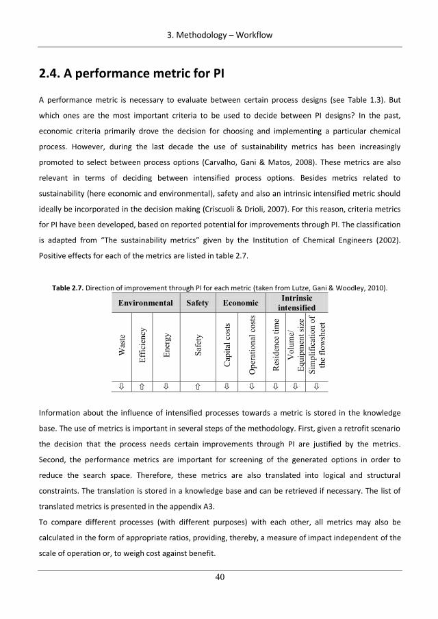
3. Methodology – Workflow
40
2.4. A performance metric for PI
A performance metric is necessary to evaluate between certain process designs (see Table 1.3). But
which ones are the most important criteria to be used to decide between PI designs? In the past,
economic criteria primarily drove the decision for choosing and implementing a particular chemical
process. However, during the last decade the use of sustainability metrics has been increasingly
promoted to select between process options (Carvalho, Gani & Matos, 2008). These metrics are also
relevant in terms of deciding between intensified process options. Besides metrics related to
sustainability (here economic and environmental), safety and also an intrinsic intensified metric should
ideally be incorporated in the decision making (Criscuoli & Drioli, 2007). For this reason, criteria metrics
for PI have been developed, based on reported potential for improvements through PI. The classification
is adapted from “The sustainability metrics” given by the Institution of Chemical Engineers (2002).
Positive effects for each of the metrics are listed in table 2.7.
Table 2.7. Direction of improvement through PI for each metric (taken from Lutze, Gani & Woodley, 2010).
Environmental Safety Economic Intrinsic intensified
Was
te
Effic
ienc
y
Ener
gy
Safe
ty
Cap
ital c
osts
Ope
ratio
nal c
osts
Res
iden
ce ti
me
Vol
ume/
Eq
uipm
ent s
ize
Sim
plifi
catio
n of
th
e flo
wsh
eet
Information about the influence of intensified processes towards a metric is stored in the knowledge
base. The use of metrics is important in several steps of the methodology. First, given a retrofit scenario
the decision that the process needs certain improvements through PI are justified by the metrics.
Second, the performance metrics are important for screening of the generated options in order to
reduce the search space. Therefore, these metrics are also translated into logical and structural
constraints. The translation is stored in a knowledge base and can be retrieved if necessary. The list of
translated metrics is presented in the appendix A3.
To compare different processes (with different purposes) with each other, all metrics may also be
calculated in the form of appropriate ratios, providing, thereby, a measure of impact independent of the
scale of operation or, to weigh cost against benefit.
70
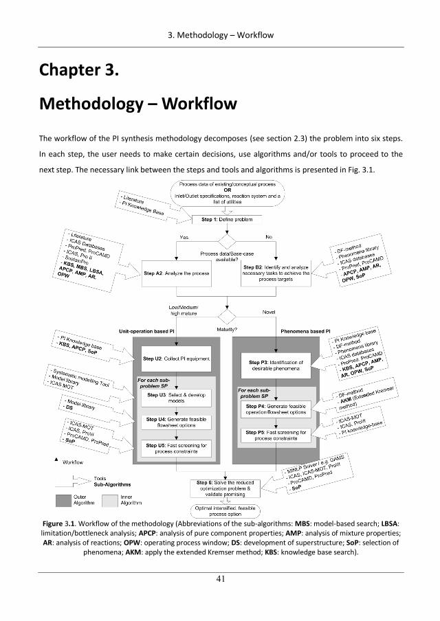
3. Methodology – Workflow
41
Chapter 3.
Methodology – Workflow
The workflow of the PI synthesis methodology decomposes (see section 2.3) the problem into six steps.
In each step, the user needs to make certain decisions, use algorithms and/or tools to proceed to the
next step. The necessary link between the steps and tools and algorithms is presented in Fig. 3.1.
Figure 3.1. Workflow of the methodology (Abbreviations of the sub-algorithms: MBS: model-based search; LBSA: limitation/bottleneck analysis; APCP: analysis of pure component properties; AMP: analysis of mixture properties; AR: analysis of reactions; OPW: operating process window; DS: development of superstructure; SoP: selection of
phenomena; AKM: apply the extended Kremser method; KBS: knowledge base search).
71
3. Methodology – Workflow
42
Steps of the unit-operation based synthesis workflow are marked with a “U” at the step number while
the steps of the phenomena-based synthesis workflow are marked with a “P”. Furthermore, there is an
outer algorithm (Steps 1-6) and an inner algorithm (Steps U3-U5 or P4-P5). The steps of the inner
algorithm are indexed with “SP” after the step number. The decision regarding which workflow is to be
followed depends on the maturity of the PI processes to be developed. For novel designs, the
phenomena-based synthesis methodology is followed while for all others, the unit-operation based is
followed.
The workflow containing all sub-steps is described in detail in sub-sections 3.1-3.2.
3.1. Workflow of the unit-operation based PI synthesis/design methodology
A brief overview of the unit operation based workflow is given in section 3.1.1 while the detailed
algorithm for each step is presented in the sections 3.1.2-3.1.9.
3.1.1. Brief overview of the workflow
The starting point of the methodology is either a base case design of an existing or a conceptual process
or input/output specification of the process.
In step 1, the synthesis/ design problem with respect to PI is defined, including the definition of the
objective function (Eq. 2.1), the process/operation scenario and the constraints that the options need to
match. Besides, the metrics for evaluation of generated options need to be selected from the available
set of metrics as well as information about desired simplification of the flowsheet (complexity) and
maturity of later considered equipment.
The objective of step 2 is to collect all data about the process, necessary to gain full understanding of
the process which is needed to identify bottlenecks/ limitations for improvement in order to search for
already existing PI strategies/equipment in a knowledge base. First, the process is translated into a task
based flowsheet as well as phenomena based flowsheet in order to identify limitations/bottlenecks of
involved phenomena in the design. In case of the selection for PI based on input/output specification, a
base-case design is built using algorithms and rules based on identification of tasks and selection of the
phenomena to fulfill the tasks. Available methods to identify bottlenecks/limitations are based on
knowledge store in a PI knowledge-base tool as well as on model-based algorithms evaluating the
performance of the process. If costs or sustainability are used as objective function, the method
72
3. Methodology – Workflow
43
described by Carvalho et al. (2007) is used. This method is based on mass and energy indicator
calculation via decomposition of the flowsheet into a process graph and indicator sensitivity analysis.
With knowledge about limitations/bottlenecks of the involved phenomena of the process, a PI
knowledge base which stores/retrieves available information (described in detail in section 3), is
consulted retrieving possible PI principles (predictive approach) and already developed PI equipment to
overcome the obtained limitations/bottlenecks for process improvement. The obtained PI solutions are
pre-screened already with respect to feasibility, e.g. process conditions, maturity and scale-up ability.
The objective of step 3 is to provide the process/operational mathematical models needed for the
subsequent calculation/evaluation steps. The necessary models may be selected from a model library,
or, if the model is not available, developed through a modeling tool using a systematic procedure
proposed by Cameron and Gani (2011). Models are important, but for them to be reliable, validation is
necessary and will require carefully collected and analyzed experimental data. All process options based
on unreliable process models are removed from the search space. Models are saved for later retrieval
into a model library.
In step 4, the objective is to generate all feasible intensified options through synthesis rules (logical
constraints, Eq. 2.2) fixing sets of binary variables within a superstructure to give the set of feasible
process options. Subsequently, structural constraints, again fixing sets of binary variables in a
superstructure, are employed to get the set of structural promising process options. Redundant options
are removed.
In step 5, all remaining PI options are fast screened using simple models (short-cut models, Eq. 2.7) or
partly rigorous simulation for matching operation constraints (Eq. 2.4). The remaining process options
are screened for additional process constraints based on performance metrics.
In step 6, the objective function (Eq. 2.1) for all remaining process options is calculated to identify the
best option. The best among these can be found through optimization (that is, fine tuning the optimal
solution). Depending on the size of the search space, the process options are optimized separately (NLP)
or through applying complex superstructure optimization methods (MINLP; see Grossmann &
Daichendt, 1996).
The reduction of the search space for the unit-operation based workflow is illustrated in figure 3.2. The
initital search space is identified in step 2 and screened through stepwise applying constraints at
different steps until the best option with respect to the objective function is identified. In general, the
workflow is designed in a flexible way such that it is possible to go backwards in order to relax
73
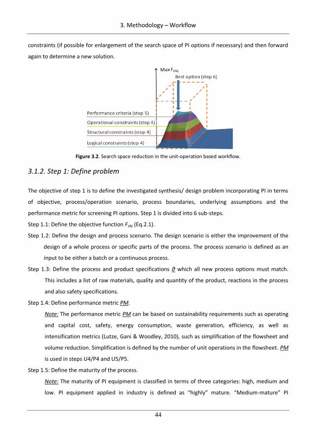
3. Methodology – Workflow
44
constraints (if possible for enlargement of the search space of PI options if necessary) and then forward
again to determine a new solution.
Figure 3.2. Search space reduction in the unit-operation based workflow.
3.1.2. Step 1: Define problem
The objective of step 1 is to define the investigated synthesis/ design problem incorporating PI in terms
of objective, process/operation scenario, process boundaries, underlying assumptions and the
performance metric for screening PI options. Step 1 is divided into 6 sub-steps.
Step 1.1: Define the objective function Fobj (Eq.2.1).
Step 1.2: Define the design and process scenario. The design scenario is either the improvement of the
design of a whole process or specific parts of the process. The process scenario is defined as an
input to be either a batch or a continuous process.
Step 1.3: Define the process and product specifications which all new process options must match.
This includes a list of raw materials, quality and quantity of the product, reactions in the process
and also safety specifications.
Step 1.4: Define performance metric PM.
Note: The performance metric PM can be based on sustainability requirements such as operating
and capital cost, safety, energy consumption, waste generation, efficiency, as well as
intensification metrics (Lutze, Gani & Woodley, 2010), such as simplification of the flowsheet and
volume reduction. Simplification is defined by the number of unit operations in the flowsheet. PM
is used in steps U4/P4 and U5/P5.
Step 1.5: Define the maturity of the process.
Note: The maturity of PI equipment is classified in terms of three categories: high, medium and
low. PI equipment applied in industry is defined as “highly” mature. “Medium-mature” PI
74
3. Methodology – Workflow
45
equipment have been run in pilot-plant facilities and have been implemented for at least two
different processes. The category “low” labels all remaining PI equipment. The maturity is used
for screening in step C2 and to decide between phenomena-based and unit-operation-based
workflow.
Step 1.6: Translate and PM into logical (Eq.2.2), structural (Eq.2.3), operational constraints (Eq.5) and
performance criteria (Eq.2.6).
Step 1.6.1: Translate items of and PM to logical constraints (Eq.2.2) by applying the rules 1.1-
1.5.
Rule 1.1: “If the defined product is not in the list of raw materials, a reaction is present.”
Rule 1.2: “If reactants enter pure the reaction has to be inside the first unit operation.”
Rule 1.3: “If more than one reaction is present and the product of one reaction (R1) is the
reactant of the second one (R2), R1 is before or at the same time as R2”.
Rule 1.4: “If the purity of the product is defined, the product outlet has to be connected to a
purification unit.”
Rule 1.5: “If the maximum number of units/type of units is fixed (simplification), ensure that
not more units are used.”
Step 1.6.2: Retrieve structural constraints (Eq.3) for the items of and PM from the knowledge-
base using a forward search procedure (see section 2.3).
Step 1.6.3: Translate items of and PM into operational constraints (Eq.2.4) or a performance
metric (Eq.2.6) by applying the rules 1.6-1.8.
Rule 1.6: “Fixed values of a specification which the process must satisfy for operational
feasibility are set to operational constraints (Eq.2.4).”
Rule 1.7: “Fixed values of a specification which the process or a part of the process must
satisfy to potentially obtain a positive improvement in the objective function are set to
operational constraints (Eq.2.4).”
Rule 1.8: “All untranslated items of and PM, after rules 1.1-1.7, are set to performance
criteria (Eq.2.6).”
Note: Examples of operational constraints by rule 1.6 are specified product concentrations
and product amount. An example of an operational constraint by rule 1.7 is a specified value
for a yield or efficiency of a reaction.
Step 1.7: Decide if Step A2 or B2 have to be followed (Rule 1.9).
Rule 1.9: “If a base-case design exists then go to step A2. Else enter step B2.”
75
3. Methodology – Workflow
46
3.1.3. Step A2: Analyze the process
The objective of step A2 is to identify the limitation of the process by analysis of the base-case design.
Step A2.1: Collect mass and energy data for the base-case design:
Step A2.1.1: Decide if the energy data of the base case design is required by using rule A2.1.
Rule A2.1: “If equations (2.1,2.4,2.6) are expressed only through mass-related design
variables X, energy data is not required.”
Step A2.1.2: Collect the mass and/or energy data of the base-case design and the phase
description of each stream. These data are provided as simulation data or directly as
operational data from a plant. The simulation data can be provided from simulation-results
of the base-case design (from process simulators like Pro\II (Pro\II, 2011) or ICASSIM in ICAS
(Gani et al., 1997).
Step A2.2: Transform the flowsheet into task-based and phenomena-based flowsheet. This involves
three sub-steps.
Step A2.2.1: Identify for each unit operation of the base-case design the task of the process. For
this a set of rules A2.2-A2.8 is used to identify the tasks: reaction, separation, heat
supply/removal, pressure increase/decrease, phase change, mixing and dividing.
Rule A2.2: “If the component masses of input and output streams of a unit are different and
the product of the reaction is the main product or a reactant of a subsequent reaction to
form the main product, then the task is a reaction.”
Rule A2.3: “If the component masses of input and output streams of a unit are different and
the reactant of the reaction is a side-product of a previous reaction, then the task is a
separation.”
Rule A2.4: “If a unit has more than one outlet stream and the outlet streams have different
compositions then a separation task is identified.”
Rule A2.5: “If more than one stream enters a unit, only one stream leaves the unit and no
reaction task has been identified, then the task of the unit is mixing.”
Rule A2.6: “If more than one outlet stream exits a unit, all with the same composition, then
the task of the unit is dividing the inlet stream.”
Rule A2.7: “If one stream enters and leaves a unit with the same composition and the same
phase but with a different temperature and/or pressure the task is heating/cooling in the
case of changing T and/or pressure increase/decrease in the case of changing P.”
76
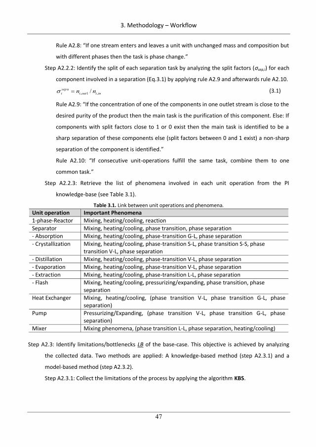
3. Methodology – Workflow
47
Rule A2.8: “If one stream enters and leaves a unit with unchanged mass and composition but
with different phases then the task is phase change.”
Step A2.2.2: Identify the split of each separation task by analyzing the split factors ( sep,i) for each
component involved in a separation (Eq.3.1) by applying rule A2.9 and afterwards rule A2.10.
, 1 ,/sepui i out i inn n (3.1)
Rule A2.9: “If the concentration of one of the components in one outlet stream is close to the
desired purity of the product then the main task is the purification of this component. Else: If
components with split factors close to 1 or 0 exist then the main task is identified to be a
sharp separation of these components else (split factors between 0 and 1 exist) a non-sharp
separation of the component is identified.”
Rule A2.10: “If consecutive unit-operations fulfill the same task, combine them to one
common task.”
Step A2.2.3: Retrieve the list of phenomena involved in each unit operation from the PI
knowledge-base (see Table 3.1).
Table 3.1. Link between unit operations and phenomena. Unit operation Important Phenomena 1-phase-Reactor Mixing, heating/cooling, reaction Separator Mixing, heating/cooling, phase transition, phase separation - Absorption Mixing, heating/cooling, phase-transition G-L, phase separation - Crystallization Mixing, heating/cooling, phase-transition S-L, phase transition S-S, phase
transition V-L, phase separation - Distillation Mixing, heating/cooling, phase-transition V-L, phase separation - Evaporation Mixing, heating/cooling, phase-transition V-L, phase separation - Extraction Mixing, heating/cooling, phase-transition L-L, phase separation - Flash Mixing, heating/cooling, pressurizing/expanding, phase transition, phase
separation Heat Exchanger Mixing, heating/cooling, (phase transition V-L, phase transition G-L, phase
separation) Pump Pressurizing/Expanding, (phase transition V-L, phase transition G-L, phase
separation) Mixer Mixing phenomena, (phase transition L-L, phase separation, heating/cooling)
Step A2.3: Identify limitations/bottlenecks LB of the base-case. This objective is achieved by analyzing
the collected data. Two methods are applied: A knowledge-based method (step A2.3.1) and a
model-based method (step A2.3.2).
Step A2.3.1: Collect the limitations of the process by applying the algorithm KBS.
77
3. Methodology – Workflow
48
Step A2.3.1.1: Prepare a list of keywords K containing the following items: the process
system, the reaction system, the tasks and the components.
Step A2.3.1.2: Apply the algorithm KBS to identify the limitations of the process. Save all
retrieved limitations in a list LB. KBS is described in section 3.3.
Step A2.3.2: Apply the algorithm MBS for a model-based search of limitations in the base-case
design.
Step A2.3.3: Identify most important limitations/bottlenecks by rule A2.11.
Rule A2.11: “If the number of items in LB is larger than 15, use the algorithm LBSA (see
section sub-algorithms) to reduce the number of LB by identification of the most sensitive
LB.”
Step A2.4: Analyze the obtained limitations/ bottlenecks LB and their corresponding tasks in the base-
case design. The objective is to identify the phenomena causing the limitation. This requires an
analysis of pure component, mixture and reaction properties together with an analysis of the
operational boundaries of the corresponding parts of the process.
Step A2.4.1: Analyze pure component properties by applying the algorithm APCP (see section
3.3).
Step A2.4.2: Analyze mixture properties by applying the algorithm AMP (see section 3.3).
Note: The following mixture properties MP are analyzed: formation of azeotropes, miscibility
gaps and the formation of an explosive atmosphere.
Step A2.4.3: Analyze reactions which have been identified to be a limitation/bottleneck by
applying the algorithm AR (see section 3.3).
Step A2.4.4: Determine the operating window of each task under investigation by applying
algorithm OPW (see section 3.3).
Step A2.5: Link a limitation/bottleneck to a task and a corresponding phenomenon outside the unit-
operation in which it occurs. This is achieved through sub-steps A2.5.1-A2.5.2.
Step A2.5.1: Identify potential tasks for additional analysis of a LB by the rules A2.12-A2.15:
Rule A2.12:”If the component is a substrate of a reaction, analyze the corresponding
reaction.”
Rule A2.13: “If the component is a solvent analyze the separation task in which it is initially
added and add it to the list LB for potential replacement of the corresponding step by PI.”
Rule A2.14: “If the component is a product of a side-reaction, add occurring side-reaction to
LB.”
78
3. Methodology – Workflow
49
Rule A2.15: “If the component is entering with a substrate then it is an impurity which is
added to LB and may be removed before entering the system.”
Step A2.5.2: Apply rule A2.16 to check if the limitation is in LB.
Rule A2.16:”If the task is already in the list LB then go to step A2.6 else add it to the list LB
and go back to step A2.4.”
Step A2.6: Select the workflow for each sub-problem SP by applying rule Workflow.
Rule Workflow: “If the maturity of the new design has been defined to be novel then enter step
P3 for the phenomena-based workflow else enter the unit-operation based workflow (see
Fig.3.1).”
3.1.4. Step B2: Identify and analyze necessary tasks to achieve the process targets
The objective of step B2 is to identify the necessary tasks to achieve the target of the process (given by
the specifications and constraints in step 1) in case a base-case design is not given. Based on a
subsequent analysis of these tasks, suitable phenomena to achieve the target of each task are identified
and selected.
Step B2.1: List all components which are known to be present in the system
Step B2.2: Describe the assignment of each component by using rules B2.1-B2.3.
Rule B2.1: “If a component is in the list of outlet components but not present or in a smaller
amount present in the inlet, the component is a product of a reaction”.
Rule B2.2: “If a component is in the list of inlet components but not present or in a smaller
amount present in the outlet, the component is a reactant of a reaction”.
Rule B2.3: “Use the descriptions given in step 1 to label components as final product, solvent,
impurity, catalyst or heating/cooling media.”
B2.3: Define all reactions in the system:
Step B2.3.1: Check the presence of all reactions
Rule B2.4: “If a component has been identified to be a product/reactant then apply Rule B2.5
else enter step B2.4.”
Rule B2.5: “Compare if all reactants/products are represented in the defined reactions. If yes
go to step B2.3.3 else enter step B2.3.2.”
Step B2.3.2: Search in the scientific literature for missing reactions and add missing components
to the list of components.
Rule B2.6: “If not all reactions can be identified then stop.”
79
3. Methodology – Workflow
50
Step B2.3.3: Identify the desirability of each reaction by applying rules B2.7-B2.9.
Rule B2.7: “If one component of a reaction is the desired product of the process or a reactant
of a subsequent reaction to form the desired product then the reaction is desirable.”
Rule B2.8: “If one component is a reactant of a reaction which is not leading to the product of
the process or not leading to a reactant of a subsequent reaction to form the desired product
but it reacts with a side-product of one of these then the reaction is a desirable side-
reaction.”
Rule B2.9: “All remaining reactions are undesirable.”
Step B2.3.4: Add all reaction tasks into a task-based flowsheet and connect all reaction tasks with
their corresponding reactants (inlet)
Step B2.3.5: Apply the algorithm AR to analyze the reaction phenomena
Step B2.4: Identify necessary separation/mixing/heat supply/removal tasks for each outlet
Step B2.4.1: Identify necessary tasks to achieve the defined targets of the process:
Rule B2.10: “If a component has to leave the process in a composition not matching the
outlet of the reaction tasks then add a separation task to achieve the desired product”.
Rule B2.11: “If components are leaving a task which is not connected to another task and the
component is defined not to leave the process then ensure the recycle into the task in which
the component is needed.”
Rule B2.12: “If a component has achieved a desired purity but the stream is in a the wrong
state, pressure and/or temperature then add a phase change, a pressure changing and or
temperature changing task into the task-based flowsheet”.
Step B2.4.2: Identify suitable phenomena by applying APCP and then AMP.
Step B2.4.3: Select potential best phenomena for each task by using the sub-algorithm SoP.
Step B2.4.4: Add all identified limitations due to the determination of the operating window in the
algorithm SoP to the list LB. Add possible outlet components to each task.
Step B2.5: Identify additional necessary tasks based on the results of step B2.4.
Rule B2.14: ”If a new component is added through one of the tasks add this component to the list
of components and go back to step B2.1.”
Rule B2.15: ”If the desired specification of a stream cannot be achieved by the identified
phenomena behind the task then add a new task and go back to step B2.4.1.”
Step B2.6: Select the workflow for each sub-problem SP by applying rule Workflow.
80
3. Methodology – Workflow
51
Rule Workflow: “If the maturity of the new design has been defined to be novel then enter step
P3 for the phenomena-based workflow else enter the unit-operation based workflow (see
Fig.3.1).”
3.1.5. Step U2: Collect PI equipment
Step U2.1: Collect potential PI equipment: The available information is used to generate a list of
candidate intensified equipment (step U2.1.1) through which the identified process limitations
can be overcome (U2.1.2).
Step U2.1.1: Prepare a list of keywords KPI for PI equipment search including all identified
limitations/bottlenecks and the phenomena to be enhanced.
Step U2.1.2: Apply the algorithm KBS to identify the limitations of the process. Save retrieved
equipment in a list .
Step U2.2: Pre-screen candidate PI equipment for feasibility and maturity: The objective of this step is to
remove all PI equipment which are not feasible for the process.
Step U2.2.1: Retrieve information about the necessary conditions for feasibility and maturity of
each PI equipment from the PI knowledge-base by applying the algorithm KBS. The following
matching criteria are used: involved phases, operating windows of integrated phenomena,
reaction phase (if existent), binary ratio in pure component properties, heat of reaction (if
existent). Additionally, retrieve the maturity of the PI equipment from the knowledge base.
Step U2.2.2: Collect and calculate necessary differences in pure component properties using the
algorithm APCP.
Step U2.2.3: Screen candidate PI equipment for feasibility using rule U2.1.
Rule U2.1: “For each candidate PI equipment (from step U2.1.2), compare all matching
criteria (see step U2.2.1) with the process conditions/boundaries (from step A2.4). If they
are not matching or fulfilled then remove the PI equipment from the search space.”
Step U2.2.4: Screen candidate PI equipment for maturity using rule U2.1-U2.3.
Rule U2.2: “If the maturity of the process is selected to be “high” then select external media
(solvent, membrane) by entering the sub-algorithm SoP and apply only step SoP.4.”
Rule U2.3: “If a solvent system is in the search space, the process is continuous and waste
and/or operational costs have been selected as performance metric then apply APCP for
known solvents (rule U2.2) to identify separation systems for solvent recycle using Jakslands
method else add a blank task for solvent recycle into the flowsheet. Add for those, a priori,
81
3. Methodology – Workflow
52
distillation as the separation system because the solvent can be tuned to match the
necessary pure component properties.”
Step U2.3: Identify sub-problems.
Step U2.3.1: Identify sub-problems by rule U2.4.
Rule U2.4: “If for a task or a set of tasks fixed inlet and outlet streams have been defined and
the identified PI equipment in the search space are not integrating one of these tasks with a
task outside, a sub-problem SP is identified. Else, no sub-problem is identified.”
Step U2.3.2: Prepare sub-list SP of candidate PI equipment to be solved in each identified sub-
problem SP.
Step U2.3.3: Enter the inner algorithm for the sub-problem SP (step U3SP).
3.1.6. Step U3SP: Select & develop models
Because data are often incomplete, models are often used to supplement the missing data. Therefore,
the objective of step U3SP is to provide the process and operational mathematical models (Eqs. 2.4 and
2.7) needed for all subsequent calculations and steps.
U3SP.1: For each missing data item, define the problem/scenario that needs to be modeled.
U3SP.2: Retrieve experimental data points Ei for the problem from scientific literature.
U3SP.3: Retrieve models from a model library. If a model is available go to step U3.5. Otherwise,
continue.
U3SP.4: Develop the necessary models through a systematic modeling procedure. In this work, the
procedure proposed by Cameron and Gani (2011) is used together with a systematic modeling
tool ICAS-MoT (Heitzig et al., 2011).
U3SP.5: Validate the model by applying sub-steps U3SP.5.1- U3SP.5.3.
U3SP.5.1: Perform a simulation with the model to check its performance against experimental
data of Ei and calculate the residual (error) to be checked by rule U3.1.
Rule U3.1: “If the residual (error) is greater than 10% then increase the counting variable cv
by 1 and go to step U3SP.5.2 to improve the model, else set cv to 0 and go to step U3SP.6.”
U3SP.5.2: Check status of the model for possible improvement by rule U3.2.
Rule U3.2: “If cv=3 then go to step U3SP.6, else go to step U3SP.4 to improve the model by
reformulation.”
U3SP.6: Save and/or remove models using rule U3.3.
82
3. Methodology – Workflow
53
Rule U3.3: “Remove non-validated models from the model library (cv=3) and remove all process
options represented by or relying on the models from the search space of process options. All
other models (cv=0) are saved in the model library.”
3.1.7. Step U4SP: Generate feasible flowsheet options
The objective of this step is to generate all process options and stepwise to screen all options by logical
constraints (Eq.2.2) to identify the subset of feasible process options NPOL. This number is further
reduced by stepwise screening (by structural constraints of Eq.2.3) to obtain the sub-set of structural
promising options NPOS. This step is divided into a number of sub-steps.
U4SP.1: Retrieve a suitable generic superstructure from the model library using rule U4.1.
Rule U4.1: “Use the information of consecutive equipment in the sub-problem (step U2.3) and
the number of maximum inlet/outlet streams of the PI equipment in the search space (step U2.3),
to search in the model library for a superstructure. If one superstructure matches these criteria
then retrieve the superstructure from the model library and enter step U4SP.3.”
U4SP.2: Develop a superstructure by using the algorithm DS (see section 3.3).
U4SP.3: Determine the number of process options NPO represented by the superstructure.
U4SP.4: Screen the generated process options NPO by stepwise applying logical constraints (Eq.2.2).
Remaining process options are NPOL.
U4SP.5: Screen the process options NPOL by stepwise applying structural constraints (Eq.2.3). Remaining
process options are NPOS.
U4SP.6: Check if the search space is empty by applying rule U4.2- U4.3.
Rule U4.2: “If NPOL=0 and SP<SPmax then go to U3SP.1 to solve the next sub-problem (SP=SP+1)
else if NPOL=0 and SP=SPmax then stop. Else (NPOL>0) check rule U4.3.”
Rule U4.3: “If NPOS=0 and SP<SPmax then go to U3SP.1 to solve the next sub-problem (SP=SP+1)
else if NPOS=0 and SP=SPmax then go to step 1, change PI metric PM and start again. Else
(NPOS>0) continue.”
3.1.8. Step U5SP: Fast screening for process constraints
The objective of step U5 is to identify the set of PI process options that match the operational
constraints by solving the short-cut model (Eq.2.7) and the operational constraints (Eq.2.4)
simultaneously. From these the most promising PI options are identified by calculating the performance
criteria (Eq.2.6) and subsequently ranked.
83
3. Methodology – Workflow
54
U5SP.1: Solve operational constraints (Eq.2.4) and the short-cut process model (Eq.2.7) for each of the
remaining process options to determine a feasible set of process variables X. This step is divided
into five sub-steps.
U5SP.1.1: Determine the degree(s) of freedom DoF of the model (Eqs.2.4&2.7).
U5SP.1.2: Specify initial process variables X to match DoF for each of the remaining process
options.
Rule U5.1: “If a solvent or membrane need to be selected then enter the sub-algorithm SoP
and apply steps SoP.4-SoP.7 to identify suitable solvents which match the operational
constraints it is screened for.”
U5SP.1.3: Solve process model (Eq. 2.4) to identify a set of process variables satisfying the
operational constraints (Eq.2.7).
U5SP.1.4: Remove redundant process options by rule U5.2.
Rule U5.2: “If a feasible set of process variables does not exist, remove the process option
from the number of remaining process options. Remaining process options are NPOO.”
U5SP.1.5: Check for necessity of relaxation of constraints by rule U5.3”.
Rule U5.3: “If NPOO=0 and SP<SPmax then go to U3SP.1 to solve the next sub-problem
(SP=SP+1) else if NPOO=0 and SP=SPmax then go to step 1, change PI metric PM and start
again. Else (NPOO>0) continue.”
U5SP.2: Identify the set of most promising options through performance screening NPOP:
U5SP.2.1: For each of the remaining process options in NPOO, calculate the performance metric p
(Eq.2.6) from the set of process variables X determined in step U5SP.1.3.
U5SP.2.2: Rank all process options according to p and select the most promising options.
The number of promising process options is NPOP.
U5SP.2.3: Check for necessity of screening by Fobj (Step U5SP.3) by rule U5.4.
Rule U5.4: “If the objective function Fobj (Eq.2.1) is not selected for screening with short-cut
process models (Eq.2.7), go to U5SP.4.”
U5SP.3: Screen by Fobj (Eq.2.1).
U5SP.3.1: Calculate the objective function Fobj (Eq.2.1).
U5SP.3.2: Rank all process options according to Fobj and select the most promising options.
The number of promising options is NPOP.
U5SP.4: Check if all sub-problems SP have been solved (Rule U5.5- U5.6).
84
3. Methodology – Workflow
55
Rule U5.5: “If the number of remaining options is below 10 but higher than 2 then decide (user
input) to repeat the screening through steps U5SP.1- U5SP.3 by complex models.”
Rule U5.6: “If SP=SPmax and if SP>1 then go to step U5SP.5, else (SP=SPmax and SP=1) go to step
6. Else (SP<SPmax) return to step U3SP.1 for the next sub-problem (SP=SP+1) to be solved.”
U5SP.5: Collect the obtained solutions of each sub-problem SP and go to step U4SP.1.
3.1.9. Step 6: Solve the reduced optimization problem and validate promising
The objective of this step is to identify the best PI process option by optimization of the objective
function Fobj with respect to logical, structural and operational constraints as well as the process model
(Eqs.2.1-2.6) simultaneously.
Step 6.1: Identify the set of most promising process options by solving an MINLP problem (if necessary).
The objective is to reduce the number of remaining options if this is necessary.
Step 6.1.1: Decide if this step is necessary by applying rule 6.1.
Rule 6.1: “If the search space NPOP is smaller than 10 then do not solve an MINLP problem
and go to step 6.2.”
Step 6.1.2: Set-up and solve an MINLP problem (Eqs.2.1-2.4,2.7). For this, the MINLP solver tool
GAMS (GAMS, 2011) is used.
Step 6.1.3: Select the best 5 process options (NPOMINLP).
Step 6.2: For each process option, solve separately the reduced optimization problem (Eqs.2.1-2.5).
Rule 6.2: “If a solvent or membrane need to be selected then enter the sub-algorithm SoP and
apply steps SoP.4-Sop.7 to identify suitable solvents which match the desired operational
constraints for the solvent system.”
Step 6.3: Rank all options by their objective function and select the best one.
Step 6.4: Validate the result from step 6.3 by rigorous simulation.
3.2. Workflow of the phenomena based PI synthesis/design methodology
In this section, first, a brief overview of the workflow is given in section 3.2.1 while the detailed
algorithm for each step is given in the sections 3.2.2-3.2.8.
85
3. Methodology – Workflow
56
3.2.1. Brief overview of the workflow
Similar to the unit-operation based workflow (section 3.1), the starting point of the methodology is
either a base case design of an existing or a conceptual process or input/output specifications of the
process. Therefore, step 1 is the same as for the unit-operation based workflow (section 3.1.2).
The objective of step 2 is to collect all data about the process, necessary to gain full understanding of
the process which is needed to identify bottlenecks/limitations and the responsible phenomena for
improvement. This step is the same as for the unit-operation based workflow except for the search for
existing PI equipment in a knowledge base (which is done in the unit-operation based method).
In step 3, the analysis of the process phenomena and the identified limitation/bottleneck are used for
identification of desirable phenomena or desirable tasks to be integrated in order to overcome the
limitation/bottleneck. For each PI possibility, the best phenomena fulfilling the desired PI are identified
and selected. Output of this step is the initital search space of necessary and desirable phenomena
within the process.
In step 4, all phenomena are interconnected to form SPB’s and screened for best performance. Based on
connectivity rules SPB’s are inserted into stages to form operations. For this, the number of stages as
well as their interconnection (co-current, counter-current, cross-current) to fulfill the necessary tasks
needs to be determined. With this information, the SPB’s are inserted into generic superstructures to
form phenomena-based process options. The process options are screened by logical and structural
constraints (Eq. 2.2-2.3).
In step 5, all remaining PI options are first screened for operation constraints (Eq. 2.4). The remaining
process options are screened for additional process constraints based on performance metrics
(Eq.2.6-2.7). The remaining phenomena based process options are transformed to units using a set of
rules to be subsequently screened by additional operational constraints as well as performance metrics
at the unit operational level.
In step 6, the best option among the remaining process options is identified using the step 6 as for the
unit-operation based workflow.
The reduction of the search space for the phenomena-based workflow is illustrated in Figure 3.3. The
initital search space is identified in step 3 and stepwise reduced through applying constraints at different
steps until the best option with respect to the objective function is identified. In general, the unit-
operation based search space is part of the phenomena based search space. The reason is that from the
phenomena all different types of units can be potentially synthesized. Comparing, figure 3.2 and figure
86
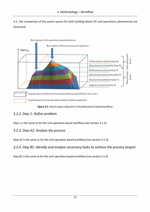
3. Methodology – Workflow
57
3.3., the comparison of the search spaces for both building blocks (PI unit-operations, phenomena) are
illustrated.
Figure 3.3. Search space reduction in the phenomena based workflow.
3.2.2. Step 1: Define problem
Step 1 is the same as for the unit-operation based workflow (see section 3.1.2).
3.2.3. Step A2: Analyze the process
Step A2 is the same as for the unit-operation based workflow (see section 3.1.3).
3.2.4. Step B2: Identify and analyze necessary tasks to achieve the process targets
Step B2 is the same as for the unit-operation based workflow (see section 3.1.4).
87
3. Methodology – Workflow
58
3.2.5. Step P3: Identification of desirable phenomena
The objective is to identify additional phenomena for synthesis of flowsheets which match the targets
defined in step 1 and improve the necessary phenomena (identified in step 2). For the selection of the
most promising phenomena, property analysis of single components and mixtures of components as
well as reactions in the system are needed.
P3.1: Identify desirable tasks as well as phenomena PI to enhance the existing necessary process
phenomena using sub-steps P3.1.1-P3.1.3.
P3.1.1: Prepare a list of keywords KPI for identification of PI possibilities including all identified
limitations/bottlenecks, tasks and the corresponding objective for PI (Fobj, PM).
P3.1.2: Apply the algorithm KBS to identify the phenomena to be targeted for enhancment
achieving the desired process improvement within a task.
P3.1.3: Apply the algorithm KBS to identify additional desirable tasks of the process.
P3.2: Use algorithm APCP to identify potential phenomena for each item of PI identified in step P3.1.
P3.3: Use algorithm AMP to identify potential phenomena for each item of PI concerning mixture
properties.
P3.4: Identify reaction phenomena if identified as additional desirable task
P3.4.1: Check if a reaction task is identified (Rule P3.1)
Rule P3.1: “If a reaction task is identified then enter step P3.4.2 else enter step P3.5.”
P3.4.2: Retrieve reaction data from databases/scientific literature by using the purpose of the task
as the keyword.
Note: If a reaction task is identified for separation of a component then search for reactions
with this component as a reactant.
P3.4.3: Enable phenomena applying rule P3.2.
Rule P3.2: “If a reaction or reactions have been identified in step P3.4.2 then add phenomena
for each of these reactions else go to step P3.5.”
P3.4.4: Use algorithm AR to analyze/compare/select potential reaction phenomena blocks for
each task.
P3.5: Enter sub-algorithm SoP to select the best phenomena for each for each item of PI.
P3.6: Retrieve accompanying phenomena information from the knowledge base and select
accompanying phenomena from the phenomena library for each identified phenomenon.
88
3. Methodology – Workflow
59
Note: Table 2.4 gives an overview of necessary connections to accompanying phenomena for each
phenomenon.
P3.7: Apply the sub-algorithm OPW to determine the operating window for each phenomenon.
P3.8: Identify sub-problems.
P3.8.1: Identify sub-problems by rule P3.3.
Rule P3.3: “If all necessary tasks have been identified to be potentially integrated then one
problem needs to be solved (SP=1). Else, the number of sub-problems (SP) to be solved is
equally to the number of tasks which can be solved separately.”
P3.8.2: Prepare list SP of integrated tasks and their corresponding phenomena to be solved in
each identified sub-problem SP.
3.2.6. Step P4SP: Generate feasible operation/flowsheet options
Inlet to this step is the initial search space of identified phenomena (nP,tot). In step P4, phenomena are
connected to simultaneous phenomena building blocks SPB’s. SPB’s are connected to form unit
operations and unit operations are combined to form process flowsheets. Between each scale,
screening steps are performed to identify the feasible sub-set. To connect SPB’s to operations, the
number of stages to achieve a process target is identified by the extended Kremser method (explained
in detail in section 3.4). With the knowledge of the number of necessary stages, the SPB’s are connected
using generic superstructures (from a model library). This step is illustrated in Figure 3.4.
89
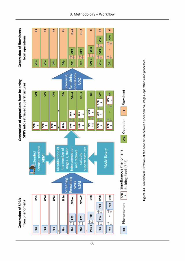
3. Methodology – Workflow
60
Figu
re 3
.4. G
raph
ical
Illu
stra
tion
of th
e co
nnec
tion
betw
een
phen
omen
a, st
ages
, ope
ratio
ns a
nd p
roce
sses
.
90
3. Methodology – Workflow
61
P4SP.1: Generate all feasible simultaneous phenomena building blocks SPB from the phenomena in the
search space:
P4SP.1.1: Identify the maximum number of phenomena within an SPB nP,max by using table 2.6.
Note: Each phenomenon can only be present once in an SPB. Opposite energy transfer
phenomena such as heating and cooling or pressurizing and expanding and different mixing
phenomena such as perfectly mixed and flow mixing can only be present once within an SPB.
A dividing phenomenon is defined to be one stage itself.
P4SP.1.2: Interconnect all phenomena in the search space to SPB’s by using the connectivity rules
for each phenomenon (see table 2.6) stored in the knowledge base.
The theoretical maximum number of SPB ‘s can be calculated by giving the total number of
phenomena in the search space nP,tot and the maximum number of phenomena within an SPB
nP,max (from step P4.1.1) using the equation 3.2:
,max,
max1 ,
1 !1
1 ! !
PnP tot
k P tot
nNSPB
n k k (3.2)
Note: The equation has been developed from the basis that a dividing phenomenon is always
a single SPB and therefore one option is added. The use of the equation is illustrated through
an example which is easy to follow. Assuming, the following phenomena in the search space
(nP,tot=4): Mixing (A), Heating (B), Pressurizing (C) and dividing (D), the maximum number of
phenomena within an SPB is nP,max=3 (dividing is an SPB on its own) and the total number of
phenomena is nP,tot=4. Hence, it gives 8 options (A=B=C, A=B, B=C, A=C, A, B, C, D) or with the
equation:
,max
,max
,max
1 , , /
3 2 1
1 ! 3 2 1 3 2 1 3 2 11 1 8(1) (3 2 1) (1) (2 1) (2 1) (1)1 ! !
P
P
nP tot
k P tot w oD
k n k k
nNSPB
n k k (1) (3 2 1) (1) (2 1) (2 1) (1)(3 2 1) (1) (2 1) (2 1)(3 2 1) (1) (2 1) (2 1)
P4SP.1.3: Screen the SPB by connectivity rules for matching operating windows of the involved
phenomena (retrieved from the knowledge-base). The number of remaining feasible stage
building blocks is NSPB.
P4SP.2: Analyze the performance of each SPB to determine the potential connections of those within
stages to fulfill a task.
This is achieved by applying the sub-steps P4.2.1-P4.2.7.
P4SP.2.1: Select for each SPB the identification and application of the necessary tools for
identification of the configuration by applying rules P4.1- P4.2.
91
3. Methodology – Workflow
62
Rule P4.1: “If the task under investigation is a separation then: for all SPB containing phase
transition phenomena enter step P4SP.2.2; and for all SPB containing a reaction and no phase
transition specify the maximum conversion (determined in step P3.4.4) as outlet
specification. Else the task is not fulfilled by the SPB.”
Rule P4.2: “If the task under investigation is a reaction then: for all SPB containing a reaction
phenomenon specify the maximum conversion (determined in step P3.4.4) as outlet
specification; and for all SPB containing phase transition and reaction phenomena enter step
P4SP.2.2. Else the task is not fulfilled by the SPB.”
P4SP.2.2: Calculate the phase diagram for each SPB containing a phase-transition phenomenon.
Rule P4.3: “If no reaction is involved then select an appropriate thermodynamic model for
the liquid and the vapor phase and calculate a phase diagram. Else use the element-based
method given by Perez-Cisneros et al. (1997,2003; see also section 4.5) to calculate reactive
phase diagrams.”
P4SP.2.3: Identify the key component for the SPB.
Rule P4.4: “The key component is defined to be the component which needs to be
recovered/formed based on the specification as the purpose of the task under investigation.”
P4SP.2.4: Apply the DF method (Bek-Pedersen & Gani, 2004) to determine minimum reflux
Rmin.(see section 4.5).
P4SP.2.5: For each SPB (including a phase transition phenomenon) apply the Kremser method
using the sub-algorithm AKM to identify the number of stages for counter-flow, co-current-
flow and cross-flow and the potential outlets.
P4SP.2.6: Compare all SPB in their performance (outcome and number of stages) to select the flow
connection (counter-flow, co-current-flow and cross-flow) by using rules P4.5-P4.8.
Rule P4.5: “Remove flow connections which are not fulfilling the tasks specifications.”
Rule P4.6: “If the difference between the minimum number of stages between the first and
the second lowest is larger than 10% then select only the first flow characteristic. Else apply
rule P4.7.”
Rule P4.7: “If the task is a reaction and can be achieved by one SPB within one stage then
select crossflow-current. Else apply Rule P4.8.”
Rule P4.8: “If the task is a separation and simplification and volume are selected as
performance metric then select counter-current characteristics.”
92
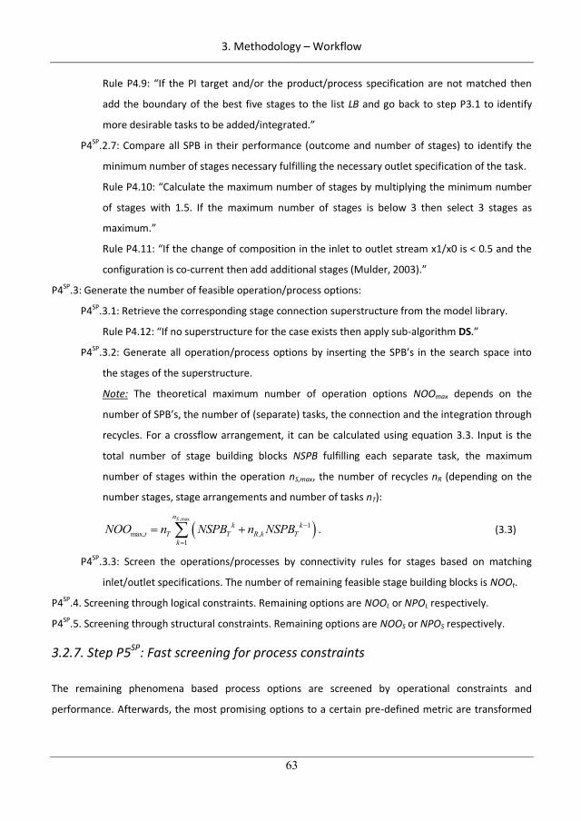
3. Methodology – Workflow
63
Rule P4.9: “If the PI target and/or the product/process specification are not matched then
add the boundary of the best five stages to the list LB and go back to step P3.1 to identify
more desirable tasks to be added/integrated.”
P4SP.2.7: Compare all SPB in their performance (outcome and number of stages) to identify the
minimum number of stages necessary fulfilling the necessary outlet specification of the task.
Rule P4.10: “Calculate the maximum number of stages by multiplying the minimum number
of stages with 1.5. If the maximum number of stages is below 3 then select 3 stages as
maximum.”
Rule P4.11: “If the change of composition in the inlet to outlet stream x1/x0 is < 0.5 and the
configuration is co-current then add additional stages (Mulder, 2003).”
P4SP.3: Generate the number of feasible operation/process options:
P4SP.3.1: Retrieve the corresponding stage connection superstructure from the model library.
Rule P4.12: “If no superstructure for the case exists then apply sub-algorithm DS.”
P4SP.3.2: Generate all operation/process options by inserting the SPB’s in the search space into
the stages of the superstructure.
Note: The theoretical maximum number of operation options NOOmax depends on the
number of SPB’s, the number of (separate) tasks, the connection and the integration through
recycles. For a crossflow arrangement, it can be calculated using equation 3.3. Input is the
total number of stage building blocks NSPB fulfilling each separate task, the maximum
number of stages within the operation nS,max, the number of recycles nR (depending on the
number stages, stage arrangements and number of tasks nT):
,max1
max, ,1
Snk k
t T T R k Tk
NOO n NSPB n NSPB . (3.3)
P4SP.3.3: Screen the operations/processes by connectivity rules for stages based on matching
inlet/outlet specifications. The number of remaining feasible stage building blocks is NOOt.
P4SP.4. Screening through logical constraints. Remaining options are NOOL or NPOL respectively.
P4SP.5. Screening through structural constraints. Remaining options are NOOS or NPOS respectively.
3.2.7. Step P5SP: Fast screening for process constraints
The remaining phenomena based process options are screened by operational constraints and
performance. Afterwards, the most promising options to a certain pre-defined metric are transformed
93
3. Methodology – Workflow
64
to unit operations using a set of rules. These options are additionally screened by operational
constraints and performance on the unit-operation level.
P5SP.1: Solve operational constraints (Eq.2.4) and the short-cut process model (Eq.2.7) for each of the
remaining process options to determine a feasible set of variables X. This step is divided into five
sub-steps.
P5SP.1.1: Determine the degrees of freedom DoF of the model (Eqs.2.4&2.7).
P5SP.1.2: Specify process variables X not included in the operational constraints to match DoF for
each of the remaining process options.
P5SP.1.3: Solve process model (Eq. 2.4) to identify a set of process variables satisfying the
operational constraints (Eq.2.7).
P5SP.1.4: Remove redundant process options by rule P5.1.
Rule P5.1: “If the operational constraints are not satisfied then remove the option from the
search space. Remaining options are NOOO or NPOO respectively.”
P5SP.2: Identify the set of most promising options through performance screening NOOP or NPOP
respectively:
P5SP.2.1: For each of the remaining options, calculate the performance metric p from the set of
process variables X determined in step P5SP.1.3.
P5SP.2.2: Rank all process options according to p and select the most promising options. The
number of promising process options is NOOP.
P5SP.2.3: Check for necessity of screening by Fobj by rule P5.2.
Rule P5.2: “If the objective function Fobj is not selected for screening at the phenomena level
then go to step P5SP.3.”
P5SP.2.4: Calculate the objective function Fobj.
P5SP.2.5: Rank all process options according to Fobj and select the most promising options. The
number of promising options is NOOP or NPOP respectively.
P5.3: Identify unit operations by using the knowledge base tool. It contains of five rules and of a list of
already translated unit-operations:
Rule P5.3: “One or a series of perfectly mixed phenomena represent one or a series of continuous
stirred tanks”.
Rule P5.4: “A countercurrent series of perfectly mixed phenomena at the same pressure
represent one tank with different compartments”.
94
3. Methodology – Workflow
65
Rule P5.5: “One or a series of the same convective mixing phenomenon represent one or a series
of channel flow units”.
Rule P5.6: “A countercurrent series of the same convective mixing phenomenon at the same
pressure represent one tank with different compartments”.
Rule P5.7: “If rules P5.4 or P5.6 are valid and a series of the same phase transition phenomena
also occur, the unit is a column.”
Rule P5.8: “If a dividing phenomenon is splitting a stream into two parallel streams connected to
the same type and the same sequence of SPB then it enables to split the volume of the unit into
an arbitrary number of parallel units.”
P5SP.4: Calculate additional operational constraints, performance metric and/or objective function Fobj
on the unit operation level (same steps than in step P5SP.1- P5SP.2, just at the unit operation level).
P5SP.5: Check if all sub-problems SP have been solved (Rule P5.9).
Rule P5.9: “If SP = SPmax and if SP > 1 then go to step P5SP.6, else (SP = SPmax and SP = 1) go to
step 6. Else (SP < SPmax) return to step P4SP.1 for the next sub-problem (SP = SP + 1) to be
solved.”
P5SP.6: Generate the number of process flowsheet options:
P5SP.6.1: Generate the theoretical maximum number of process flowsheet options:
The theoretical maximum number of operation options NPOmax with only possible
connections per operation can be calculated by giving the total number of necessary tasks
nt,max, under investigation and the maximum operations for each task NOOt using the
following equation:
,max
max1
tnt
tt
NPO NOO (3.4)
P5SP.6.2: Screen the operations by connectivity rules for operations (retrieved from the
knowledge-base) and matching operating windows. The number of remaining process
options is NPO.
P5SP.6.3: Enter step P4SP.5.
3.2.8. Step 6: Solve the reduced optimization problem and validate promising
Step 6 is the same as for the unit-operation based workflow (see section 3.1.9).
95
3. Methodology – Workflow
66
3.3. Sub-algorithms
3.3.1. MBS (model-based search)
The algorithm MBS has been developed to determine the limitations/bottlenecks through a model-
based search. Four steps are needed.
MBS.1: Calculate the objective function Fobj (Eq.2.1), operational constraints (Eq.2.4) and performance
criteria i (Eq.2.6) for the whole process and for each task of the process of the base-case design.
MBS.2: Rank the tasks based on their contribution to the Fobj (Eq.2.1) and for each i (Eq.2.6). Add those
tasks to the list LB which contribute mostly to a negative performance of the base-case design.
MBS.3: Add all tasks to the potential list of limitations/bottlenecks LB in which an operational constraint
is violated.
MBS.4: Check if operating costs or sustainability have been defined as performance criteria i,
operational constraints and/or objective function Fobj in step 1. If yes, calculate and analyze mass
and energy indicators by applying the method and the tool “SustainPro” (see section 4.7) from the
ICAS-toolbox developed by Carvalho et al. (2008). If not, leave MBS.
3.3.2. LBSA (limitation/bottleneck sensitivity analysis)
The algorithm LBSA has been developed for quick determination of the limitations/bottlenecks which
have the potential to improve the process performance most when this task is enhanced.
LBSA.1: Replace all unit operations with their corresponding performance factors based on mass and/or
energy. Table 3.2 gives the expression of the performance factors (Eqs.3.1,3.5-3.11) for each
corresponding unit-operation.
96
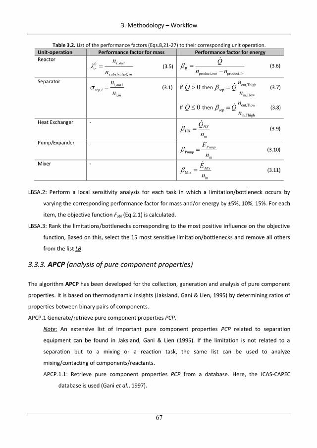
3. Methodology – Workflow
67
Table 3.2. List of the performance factors (Eqs.8,21-27) to their corresponding unit operation. Unit-operation Performance factor for mass Performance factor for energy Reactor
inAsubstrate
outir n
n
,
,0 (3.5) Rproduct, product,out in
Qn n
Q (3.6)
Separator , 1
,,
i outsep i
i in
nn
(3.1) If 0Q 0Q then out,Thighsep
in,Tlow
nQ
nout,Thighn
Q (3.7)
If 0Q 0Q then out,Tlowsep
in,Thigh
nQ
nout,Tlown
Q (3.8)
Heat Exchanger - HX
in
HXQn
HXQH (3.9)
Pump/Expander - Pump
in
PumpEnPEP (3.10)
Mixer - Mix
in
MixEn
MiEM (3.11)
LBSA.2: Perform a local sensitivity analysis for each task in which a limitation/bottleneck occurs by
varying the corresponding performance factor for mass and/or energy by ±5%, 10%, 15%. For each
item, the objective function Fobj (Eq.2.1) is calculated.
LBSA.3: Rank the limitations/bottlenecks corresponding to the most positive influence on the objective
function, Based on this, select the 15 most sensitive limitation/bottlenecks and remove all others
from the list LB.
3.3.3. APCP (analysis of pure component properties)
The algorithm APCP has been developed for the collection, generation and analysis of pure component
properties. It is based on thermodynamic insights (Jaksland, Gani & Lien, 1995) by determining ratios of
properties between binary pairs of components.
APCP.1 Generate/retrieve pure component properties PCP.
Note: An extensive list of important pure component properties PCP related to separation
equipment can be found in Jaksland, Gani & Lien (1995). If the limitation is not related to a
separation but to a mixing or a reaction task, the same list can be used to analyze
mixing/contacting of components/reactants.
APCP.1.1: Retrieve pure component properties PCP from a database. Here, the ICAS-CAPEC
database is used (Gani et al., 1997).
97
3. Methodology – Workflow
68
APCP.1.2: Predict pure component properties if missing properties not available. Here, the
property prediction tool “ProPred” from the ICAS toolbox (Gani et al., 1997) is used.
APCP.2: Calculate the ratios of properties between binary pairs of components rkl (Eq. 3.12).
/kl k lr PCP PCP (3.12)
With k l and k,l = 1...n with n: number of components.
APCP.3: Retrieve for each phenomenon within a limiting task the important pure component properties
from the PI database (apply only for the identification of a limitation).
APCP.4: Analyze the ratios of properties between binary pairs involved in each phenomenon by applying
the rules APCP.1- APCP.9 (apply this step only for the identification of a limitation).
Rule APCP.1: “If the binary ratio of a phase transition phenomenon in the corresponding PCP is
close to unity the separation is difficult and responsible for a limitation.”
Rule APCP.2: “If the binary ratio of the Octanol/Water partition coefficient Log(Kow), the water
solubility Log(Ws) and/or the solubility parameter is much larger than 1 in any 1-phase mixing
phenomenon, then a phase split of the components may occur which is responsible for low
contacting/mixing of the involved components and therefore responsible for a limitation caused
by the mixing phenomenon.”
Rule APCP.3: “If the components are highly viscous and the limitation has been identified to be a
high energy consumption in this task, then the mixing phenomenon is identified to be one source
for it.”
Rule APCP.4: “If the components are highly viscous and the limitation has been identified to be a
low contacting time, then the mixing phenomenon may not be ideal and is identified to be one
source for it.”
Rule APCP.5: “Heat transfer phenomena may be limited when heat capacities are large. Further
studies are important in AR and OPW.”
Rule APCP.6: “If Tin Tout in the task under investigation and the heat capacities are very small,
temperature control may be difficult which means that the heat and mixing phenomena are
limiting the process operation. Further studies are enabled in AR and OPW.”
Rule APCP.7: ”If a component has to be dissolved into another phase and the corresponding
binary ratio of the phase transition phenomenon is large then the phase transition phenomenon is
responsible for a limitation.”
98
3. Methodology – Workflow
69
Rule APCP.8: ”If the ratio of the pure component properties of phase transition phenomenon
which needs thermal energy (e.g. relative volatility) is large and the energy is used as one criteria
then this is one reason for the limitation.”
Rule APCP.9: “If the binary ratio in a phase transition is large but the key components are very
dilute then a large residence time/high contacting/large amount of solvent/high energy amount
(depending on the phenomena under investigation) is needed limiting the process performance.”
APCP.5: Identify suitable phase transition phenomena using rule APCP.10-APCP.11 (apply this step only
for the identification of phase transition phenomena).
Rule APCP.10: “If the binary ratio PCP is larger than 1.05 then the separation is potentially
feasible.”
Rule APCP.11: Identify for each potentially feasible separation, the corresponding phase transition
phenomenon using Table 3.3 and add it to the list of potential phase transition phenomena for the
separation task.”
3.3.4. AMP (analysis of mixture properties)
The algorithm AMP has been developed for the collection, generation and analysis of mixture
properties. This algorithm is divided into five steps.
AMP.1: Select mixture properties for analysis by the following four rules AMP.1-AMP.4:
Rule AMP.1: “If in the task vapor and liquid phases are involved then check for azeotropes.”
Rule AMP.2: “If in the task two liquid phases occur or one liquid phase but the analysis of binary
ratios of the solubility parameter showed a large difference between two components then a
detailed analysis of the miscibility is necessary.”
Rule AMP.3: “If safety has been selected as a performance metric in step 1 and a vapor/gas phase
occurs then check the formation of an explosive atmosphere.”
Rule AMP.4: “If no mixture property is selected, leave AMP algorithm.”
AMP.2: Retrieve the selected mixture property MPi from databases or the literature. Here, for
azeotropes a database in ICAS (Gani et al., 1997) is used.
AMP.3: Compute azeotropes and/or miscibility gaps using thermodynamic models describing the
involved phases:
AMP.3.1 Check if step AMP.3 is necessary by applying rule AMP.5.
Rule AMP.5: ”If no detailed information about azeotropes and/or miscibility’s has been found then
go to step AMP.3.2 else then go to step AMP.5.”
99
3. Methodology – Workflow
70
AMP.3.2: Select a thermodynamic model describing the phase relationship and retrieve parameters
from a database. For this, the ICAS-CAPEC database manager is used (Gani et al., 1997). The
selection of the thermodynamic model depends on the availability of parameters in the database.
AMP.3.3 Check if the computation of the mixture properties is possible by rule AMP.6.
Rule AMP.6: “If no complete set of parameters exists then leave AMP algorithm.”
AMP.4: Identify azeotropes and/or miscibility gaps (depending on the target) by usage of the selected
thermodynamic model.
AMP.5: Identify a phenomenon responsible for a limitation by rule AMP.7 (apply this step only for the
identification of a limitation).
Rule AMP.7: “If the process conditions are within the miscibility gap and/or close to an azeotrope
then the phenomenon is responsible for a limitation.”
AMP.6: Identify suitable phase transition phenomena using rule AMP.8 (apply this step only for the
identification of phase transition phenomena).
Rule AMP.8: “If a miscibility gap is identified then phase transition by settling is put into the search
space of phenomena.”
3.3.5 AR (analysis of reactions)
The algorithm AR has been developed for the analysis of the involved reactions. Seven steps are needed
to go through this algorithm.
AR.1: Check for application of the algorithm by rule AR.1.
Rule AR.1: “If no reaction r is in the list for limitations/bottlenecks LB then leave the AR
algorithm.”
AR.2: Collect data for reaction analysis:
AR.2.1: Collect experimental equilibrium data EEQ and/or the equilibrium constant KEQ and/or a
model for determination of KEQ by the change of the Gibbs-energy of the each reaction from
the literature.
AR.2.2: In case batch reactions are investigated, collect information about residence time from the
literature.
AR.2.3: Check if determination of the heat of reaction is required by rule AR.2.
Rule AR.2: “If energy data is not considered in Eqs.2.1-2.5 then go to step AR.3.”
AR.2.4: Retrieve the heat of formation for each component from a database. Here the ICAS-
database is used.
100
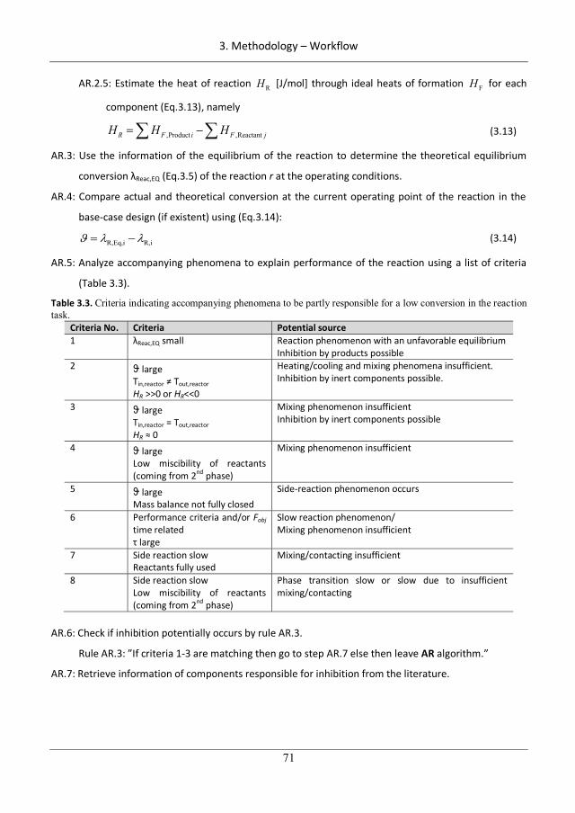
3. Methodology – Workflow
71
AR.2.5: Estimate the heat of reaction RH [J/mol] through ideal heats of formation FH for each
component (Eq.3.13), namely
,Product ,ReactantR F i F jH H H (3.13)
AR.3: Use the information of the equilibrium of the reaction to determine the theoretical equilibrium
conversion Reac,EQ (Eq.3.5) of the reaction r at the operating conditions.
AR.4: Compare actual and theoretical conversion at the current operating point of the reaction in the
base-case design (if existent) using (Eq.3.14):
R,Eq,i R,i (3.14)
AR.5: Analyze accompanying phenomena to explain performance of the reaction using a list of criteria
(Table 3.3).
Table 3.3. Criteria indicating accompanying phenomena to be partly responsible for a low conversion in the reaction task.
Criteria No. Criteria Potential source 1 Reac,EQ small Reaction phenomenon with an unfavorable equilibrium
Inhibition by products possible 2 large
Tin,reactor Tout,reactor HR >>0 or HR<<0
Heating/cooling and mixing phenomena insufficient. Inhibition by inert components possible.
3 large Tin,reactor = Tout,reactor
HR 0
Mixing phenomenon insufficient Inhibition by inert components possible
4 large Low miscibility of reactants (coming from 2nd phase)
Mixing phenomenon insufficient
5 large Mass balance not fully closed
Side-reaction phenomenon occurs
6 Performance criteria and/or Fobj time related large
Slow reaction phenomenon/ Mixing phenomenon insufficient
7 Side reaction slow Reactants fully used
Mixing/contacting insufficient
8 Side reaction slow Low miscibility of reactants (coming from 2nd phase)
Phase transition slow or slow due to insufficient mixing/contacting
AR.6: Check if inhibition potentially occurs by rule AR.3.
Rule AR.3: ”If criteria 1-3 are matching then go to step AR.7 else then leave AR algorithm.”
AR.7: Retrieve information of components responsible for inhibition from the literature.
101
3. Methodology – Workflow
72
3.3.6. OPW (operating process window)
The algorithm OPW has been developed for the determination of the operating window of each
phenomenon and the unit operations.
OPW.1: Add the maximum and minimum temperatures and pressures for each phenomenon as
operational constraints (Eq.2.4).
OPW.2: Add the miscibility boundaries and azeotropic boundaries as operational constraints (Eq.2.4) to
all phenomena running in the corresponding phase.
OPW.3: Retrieve data about stability of components, membranes and catalysts/enzymes from the
literature and add them to the operational constraints (Eq.2.4).
OPW.4: Combine the operational constraints for all phenomena involved in a unit to set the operating
window of a unit (only necessary when at the unit operational level).
OPW.5: Check the position of the current process point and apply rule OPW.1 (only necessary when sub-
algorithm is entered from step A2/B2).
Rule OPW.1: “If the operating point is on a boundary of the operating window for the temperature
and the corresponding heat phenomena have not been analyzed for a limitation yet then go to
step A2.4.1/B2.4.2 for analysis of the heat phenomena else then check rule OPW.2.”
Rule OPW.2: “If the operating point is on a boundary of the operating window for the
concentration and the corresponding mixing phenomena have not been analyzed for a limitation
yet then go back to step A2.4.1/B2.4.2 else continue.”
3.3.7. DS (development of a superstructure)
This algorithm has been developed to generate a superstructure based on the items in a search space
for a process or SP for a subproblem.
DS.1: Take the flowsheet of the base case design and add a binary variable Y to each stream.
DS.2: Take an item of / SP together with the information for which task in the flowsheet it has been
identified.
DS.3: Identify inlet and outlet streams of this item using the information of the task it is going to
perform.
DS.4: Based on the information of the two previous steps, position the item into the flowsheet and add
a binary variable Y to each stream connecting this unit.
DS.5: Delete item from / SP
102
3. Methodology – Workflow
73
DS.6: Check if all items are in the superstructure by applying rule DS.1.
Rule DS.1: “If / SP is not empty then go to step DS.2.”
3.3.8. SoP (selection of phenomena)
This algorithm has been developed to select the potentially most promising phenomena for a specific
task and to set up the intital search space of phenomena.
SoP.1: Identify the operating window of each phenomenon by OPW.
SoP.2 Predict the maximum possible (ideal solvent/membrane) number of outlets of each phase
transition phenomenon using the information about their outlet constraints and the operating
window.
SoP.3: Pre-screen phenomena by their potential performance within the operating window and check
against the defined performance metric using the rules SoP.1-SoP.4.
Rule SoP.1: “If the necessary task to be fulfilled by a phenomenon is outside of the operating
window of this phenomenon then remove the phenomenon from the search space.”
Rule SoP.2: “If the desirable task to be fulfilled by a phenomenon is outside of the operating
window of this phenomenon and the coupled task(s) then remove the phenomenon from the
search space.”
Rule SoP.3: “If efficiency, waste and/or operating costs are used as performance criteria or Fobj
then screen out the phenomena of a desirable task in which the largest amount of substrate,
product or solvent are potentially lost.”
Rule SoP.4: “If the maximum possible outlet of a phenomenon shows that the desirable task
specifications are not fulfilled without adding an additional task which is not in the list of tasks
then remove the phenomenon when the simplification is used as criterion and another
phenomenon fulfills this task without the necessity of an additional task.”
SoP.4: Collect external media (solvent, membrane) data (if necessary) from the scientific literature and
databases.
Rule SoP.5: “If no external medium has been found or the user input reveals to include a search
for new external media, then enter step SoP.5 for solvent selection and/or for membrane
selection. Else, discard phenomena and enter step SoP.7.”
SoP.5: Apply the tool ProCAMD for solvent selection (Gani et al., 2005).
Rule SoP.6: “In case of operating costs as one of the performance criteria or Fobj, add the costs to
one of the indicators for selection of the solvent.”
103
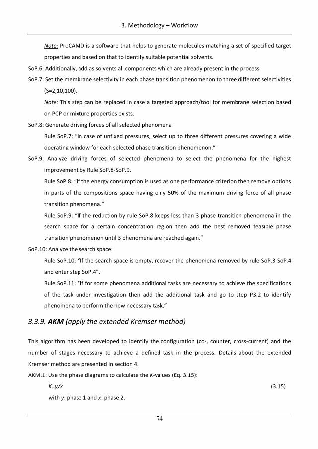
3. Methodology – Workflow
74
Note: ProCAMD is a software that helps to generate molecules matching a set of specified target
properties and based on that to identify suitable potential solvents.
SoP.6: Additionally, add as solvents all components which are already present in the process
SoP.7: Set the membrane selectivity in each phase transition phenomenon to three different selectivities
(S=2,10,100).
Note: This step can be replaced in case a targeted approach/tool for membrane selection based
on PCP or mixture properties exists.
SoP.8: Generate driving forces of all selected phenomena
Rule SoP.7: “In case of unfixed pressures, select up to three different pressures covering a wide
operating window for each selected phase transition phenomenon.”
SoP.9: Analyze driving forces of selected phenomena to select the phenomena for the highest
improvement by Rule SoP.8-SoP.9.
Rule SoP.8: “If the energy consumption is used as one performance criterion then remove options
in parts of the compositions space having only 50% of the maximum driving force of all phase
transition phenomena.”
Rule SoP.9: “If the reduction by rule SoP.8 keeps less than 3 phase transition phenomena in the
search space for a certain concentration region then add the best removed feasible phase
transition phenomenon until 3 phenomena are reached again.”
SoP.10: Analyze the search space:
Rule SoP.10: “If the search space is empty, recover the phenomena removed by rule SoP.3-SoP.4
and enter step SoP.4”.
Rule SoP.11: “If for some phenomena additional tasks are necessary to achieve the specifications
of the task under investigation then add the additional task and go to step P3.2 to identify
phenomena to perform the new necessary task.”
3.3.9. AKM (apply the extended Kremser method)
This algorithm has been developed to identify the configuration (co-, counter, cross-current) and the
number of stages necessary to achieve a defined task in the process. Details about the extended
Kremser method are presented in section 4.
AKM.1: Use the phase diagrams to calculate the K-values (Eq. 3.15):
K=y/x (3.15)
with y: phase 1 and x: phase 2.
104
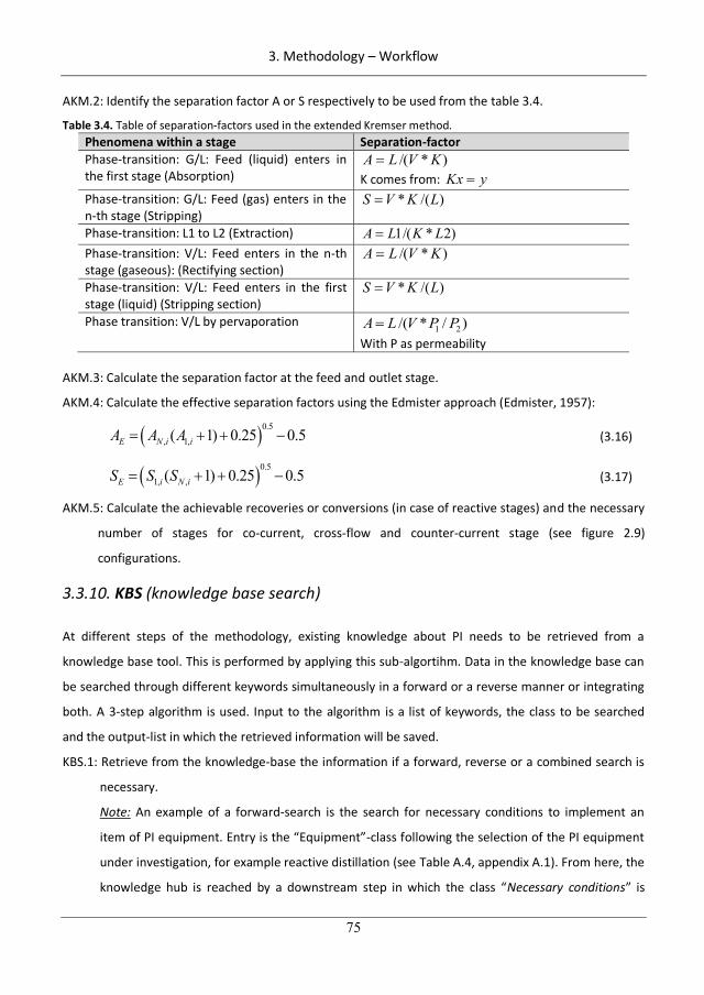
3. Methodology – Workflow
75
AKM.2: Identify the separation factor A or S respectively to be used from the table 3.4.
Table 3.4. Table of separation-factors used in the extended Kremser method. Phenomena within a stage Separation-factor Phase-transition: G/L: Feed (liquid) enters in the first stage (Absorption)
)*/( KVLA K comes from: yKx
Phase-transition: G/L: Feed (gas) enters in the n-th stage (Stripping)
* /( )S V K L
Phase-transition: L1 to L2 (Extraction) )2*/(1 LKLA Phase-transition: V/L: Feed enters in the n-th stage (gaseous): (Rectifying section)
)*/( KVLA
Phase-transition: V/L: Feed enters in the first stage (liquid) (Stripping section)
* /( )S V K L
Phase transition: V/L by pervaporation 1 2/( * / )A L V P P
With P as permeability AKM.3: Calculate the separation factor at the feed and outlet stage.
AKM.4: Calculate the effective separation factors using the Edmister approach (Edmister, 1957):
0.5, 1,( 1) 0.25 0.5E N i iA A A (3.16)
0.51, ,( 1) 0.25 0.5E i N iS S S (3.17)
AKM.5: Calculate the achievable recoveries or conversions (in case of reactive stages) and the necessary
number of stages for co-current, cross-flow and counter-current stage (see figure 2.9)
configurations.
3.3.10. KBS (knowledge base search)
At different steps of the methodology, existing knowledge about PI needs to be retrieved from a
knowledge base tool. This is performed by applying this sub-algortihm. Data in the knowledge base can
be searched through different keywords simultaneously in a forward or a reverse manner or integrating
both. A 3-step algorithm is used. Input to the algorithm is a list of keywords, the class to be searched
and the output-list in which the retrieved information will be saved.
KBS.1: Retrieve from the knowledge-base the information if a forward, reverse or a combined search is
necessary.
Note: An example of a forward-search is the search for necessary conditions to implement an
item of PI equipment. Entry is the “Equipment”-class following the selection of the PI equipment
under investigation, for example reactive distillation (see Table A.4, appendix A.1). From here, the
knowledge hub is reached by a downstream step in which the class “Necessary conditions” is
105
3. Methodology – Workflow
76
reached in which four sub-classes exist: “General process properties”, “Component properties”,
“Operational properties” and “Occurring phases”. Selecting “General process properties” gives
several items for application of reactive distillation (see Table appendix A.1) such as “Feed is
liquid or vapour or both”, “Reaction(s) is in liquid phase”, etc.
KBS.2: Search for each keyword K in the knowledge-base.
Note: An example of a reverse-search is the search for PI equipment which have been already
implemented for a certain reaction, for example esterification. Entry of the reverse search is the
“Reaction Class” (see Fig.4.1) selecting the item “esterification” (see Table A.4, appendix A.1).
Going one step reverse(back), the “equipment class” is reached (see Fig. 4.1). Examples for
implemented PI equipment for esterification reactions are reactive distillation and reactive
pervaporation (see Table A.4, appendix A.1).
KBS.3: Save retrieved items in the output-list.
106
4. Methodology – Supporting methods & tools
77
Chapter 4.
Methodology – Supporting methods & tools
The developed methodology depends on a number of supporting methods and tools (see also Figure
3.1). These are presented in sufficient details in this section.
4.1. Knowledge-base tool
At different steps of the developed workflows (section 3.1 and 3.2) knowledge about existing PI unit
operations (unit-operation based workflow) as well as PI principles (phenomena-based workflow, see
section 1.1.1 for PI principles) needs to be provided. This includes, for example, knowledge about
characteristics of existing PI equipment and their operating windows or knowledge about tasks and
phenomena which can be used to overcome a limitation within an operation. Therefore, the purpose of
the knowledge-base tool is to store and provide this necessary knowledge obtained from scientific
literature in an efficient way.
In order to structure the information in a simple, efficient and flexible way, an ontology for PI knowledge
representation has been developed (see section 4.1.1). Details on the design of ontology-based
knowledge bases as well as an overview of knowledge bases in other research areas are given by Singh
et al. (2010) and Venkatasubramanian et al. (2006). The following main items are stored in the
knowledge-base tool:
Existing PI equipment (section 4.1.2)
Knowledge for identification of PI principles (section 4.1.3)
Translated performance metric into logical, structural and operational constraints at different
levels of abstraction: unit-operation, phenomena (appendix A.3)
Rules for the transformation of phenomena into a unit-operation (see section 3.1.6; step P5SP.3)
4.1.1. Architecture of the knowledge-base
The architecture of the knowledge base is briefly explained below. Each of the main items is represented
by a knowledge hub, which branches out in several directions with stored information. The architecture
is represented for the “existing PI equipment”-item in Figure 4.1. Starting from the principles of PI on
107
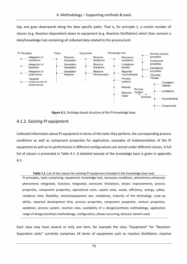
4. Methodology – Supporting methods & tools
78
top, one goes downwards along the data specific paths. That is, for principle 1, a certain number of
classes (e.g. Reaction-Separation) down to equipment (e.g. Reaction Distillation) which then connect a
data/knowledge hub containing all collected data related to this process/unit.
Figure 4.1. Ontology-based structure of the PI knowledge base.
4.1.2. Existing PI equipment.
Collected information about PI equipment in terms of the tasks they perform, the corresponding process
conditions as well as component properties for application; examples of implementation of the PI
equipment as well as its performance in different configurations are stored under different classes. A full
list of classes is presented in Table 4.1. A detailed excerpt of the knowledge base is given in appendix
A.1.
Table 4.1. List of the classes for existing PI equipment included in the knowledge base tool. PI-principles, tasks comprising, equipment, knowledge hub, necessary conditions, phenomena enhanced,
phenomena integrated, functions integrated, overcome limitations, shown improvements, process
properties, component properties, operational costs, capital costs, waste, efficiency, energy, safety,
residence time, flexibility, volume/equipment size, complexity, maturity of the technology, scale-up
ability, reported development time, process properties, component properties, mixture properties,
validation, process system, reaction class, availability of a design/synthesis methodology, application
range of design/synthesis methodology, configuration, phases occurring, devices/ solvent used.
Each class may have several or only one item, for example the class “Equipment” for “Reaction-
Separation tasks” currently comprises 24 items of equipment such as reactive distillation, reactive
108
4. Methodology – Supporting methods & tools
79
extraction and reactive pervaporation. The knowledge-base is built up in columns and rows to achieve
easy extension of the knowledge base to new PI equipment as well as new information classes.
This knowledge is necessary in step U2 (unit-operation based workflow; see section 3.1) for
identification of PI equipment to overcome limitations/bottlenecks for a targeted process improvement,
for checking of pre-feasibility and the maturity of the PI equipment in the search space as well as
properties determining the operating window and therefore also the integration of a PI equipment into
a flowsheet.
Currently, the knowledge base comprises around 12000 information items for 37 classes and 135 items
of PI equipment and internals in around 200 different process configurations. The list of PI equipment
and internals can be found in appendix A1.
4.1.3. Knowledge for identification of PI principles
An analysis of the characteristics and performance of the existing PI equipment stored in the knowledge
base has led to the development of a decision table for identification of general PI principles
independent from PI equipment to overcome a number of limitations/bottlenecks in the process. This is
used by both workflows for identification of the phenomena to be enhanced for achieving a targeted
process improvement. One of such a decision table to identify PI solutions for a number of limitations
within a reaction and a separation task is presented in Table 4.2. As an illustration, an unfavorable
equilibrium within a reaction task is considered which can be overcome by the integration of the
necessary reaction task with a separation and/or a second reaction task removing one (or more than
one) product.
109
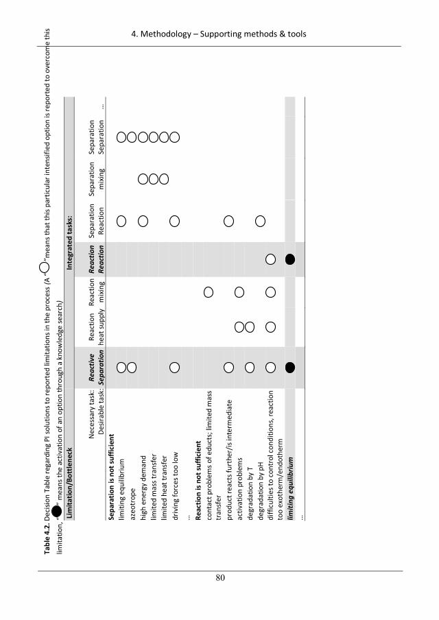
4. Methodology – Supporting methods & tools
80
Tabl
e 4.
2. D
ecisi
on T
able
rega
rdin
g PI
solu
tions
to re
port
ed li
mita
tions
in th
e pr
oces
s (A
“”m
eans
that
this
part
icul
ar in
tens
ified
opt
ion
is re
port
ed to
ove
rcom
e th
is
limita
tion,
“”
mea
ns th
e ac
tivat
ion
of a
n op
tion
thro
ugh
a kn
owle
dge
sear
ch)
Lim
itatio
n/Bo
ttle
neck
In
tegr
ated
task
s:
Nec
essa
ry ta
sk:
Desir
able
task
:Re
activ
e
Sepa
ratio
n Re
actio
n he
at su
pply
Reac
tion
mix
ing
Reac
tion
Reac
tion
Sepa
ratio
n Re
actio
n Se
para
tion
mix
ing
Sepa
ratio
n Se
para
tion
…
Sepa
ratio
n is
not s
uffic
ient
lim
iting
equ
ilibr
ium
az
eotr
ope
high
ene
rgy
dem
and
limite
d m
ass t
rans
fer
limite
d he
at tr
ansf
er
driv
ing
forc
es to
o lo
w
…
Reac
tion
is n
ot su
ffici
ent
cont
act p
robl
ems o
f edu
cts;
lim
ited
mas
s tr
ansf
er
prod
uct r
eact
s fur
ther
/is in
term
edia
te
activ
atio
n pr
oble
ms
degr
adat
ion
by T
de
grad
atio
n by
pH
diffi
culti
es to
con
trol
con
ditio
ns, r
eact
ion
too
exot
herm
/end
othe
rm
limiti
ng e
quili
briu
m
…
110
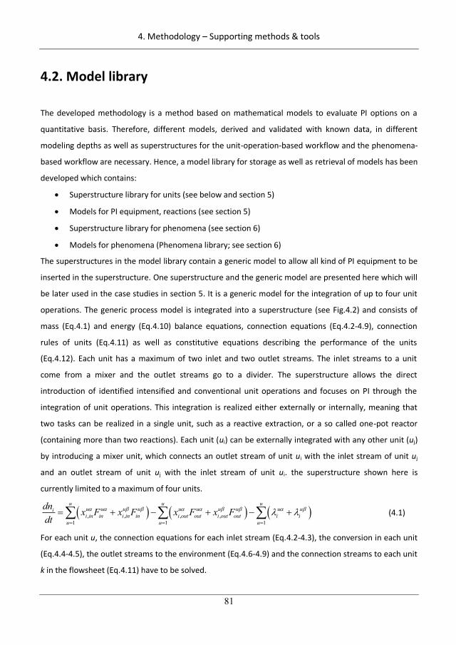
4. Methodology – Supporting methods & tools
81
4.2. Model library
The developed methodology is a method based on mathematical models to evaluate PI options on a
quantitative basis. Therefore, different models, derived and validated with known data, in different
modeling depths as well as superstructures for the unit-operation-based workflow and the phenomena-
based workflow are necessary. Hence, a model library for storage as well as retrieval of models has been
developed which contains:
Superstructure library for units (see below and section 5)
Models for PI equipment, reactions (see section 5)
Superstructure library for phenomena (see section 6)
Models for phenomena (Phenomena library; see section 6)
The superstructures in the model library contain a generic model to allow all kind of PI equipment to be
inserted in the superstructure. One superstructure and the generic model are presented here which will
be later used in the case studies in section 5. It is a generic model for the integration of up to four unit
operations. The generic process model is integrated into a superstructure (see Fig.4.2) and consists of
mass (Eq.4.1) and energy (Eq.4.10) balance equations, connection equations (Eq.4.2-4.9), connection
rules of units (Eq.4.11) as well as constitutive equations describing the performance of the units
(Eq.4.12). Each unit has a maximum of two inlet and two outlet streams. The inlet streams to a unit
come from a mixer and the outlet streams go to a divider. The superstructure allows the direct
introduction of identified intensified and conventional unit operations and focuses on PI through the
integration of unit operations. This integration is realized either externally or internally, meaning that
two tasks can be realized in a single unit, such as a reactive extraction, or a so called one-pot reactor
(containing more than two reactions). Each unit (ui) can be externally integrated with any other unit (uj)
by introducing a mixer unit, which connects an outlet stream of unit ui with the inlet stream of unit uj
and an outlet stream of unit uj with the inlet stream of unit ui. the superstructure shown here is
currently limited to a maximum of four units.
, , , ,1 1 1
u u uu u u u u u u u u uii in in i in in i out out i out out i i
u u u
dn x F x F x F x Fdt
(4.1)
For each unit u, the connection equations for each inlet stream (Eq.4.2-4.3), the conversion in each unit
(Eq.4.4-4.5), the outlet streams to the environment (Eq.4.6-4.9) and the connection streams to each unit
k in the flowsheet (Eq.4.11) have to be solved.
111
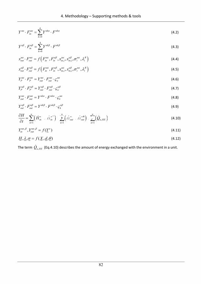
4. Methodology – Supporting methods & tools
82
4
0
u u uk ukin
k
Y F Y F (4.2)
4
0
u u uk ukin
k
Y F Y F (4.3)
, ,, , , , ,u u u u u u u Rout out in in in i in i i ix F f F F x x (4.4)
, ,, , , , ,u u u u u u u Rout out in in in i in i i ix F f F F x x (4.5)
u u u u uP P out out uY F Y F (4.6)
u u u u uP P out out uY F Y F (4.7)
u u uk uk uout out kY F Y F (4.8)
u u uk uk uout out kY F Y F (4.9)
,1 1 1
u u uu u u uin in out out u HX
u u u
H H H H H Qt HX
u u
QuH u u u uu uu u uu uu uH H H Hui i t tH H HH H HH Hu u uuu u Q (4.10)
, ,, ( )u u uin outY Y f Y (4.11)
, , ( , , )H f X d (4.12)
The term ,u HXQ HXQ (Eq.4.10) describes the amount of energy exchanged with the environment in a unit.
112
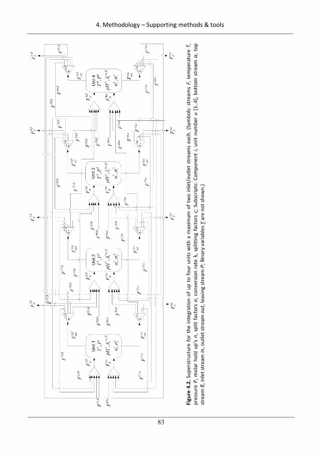
4. Methodology – Supporting methods & tools
83
Figu
re 4
.2. S
uper
stru
ctur
e fo
r th
e in
tegr
atio
n of
up
to fo
ur u
nits
with
a m
axim
um o
f tw
o in
let/
outle
t st
ream
s ea
ch. (
Sym
bols:
str
eam
s F,
tem
pera
ture
T,
pres
sure
P, m
olar
hol
d up
’s n,
spl
it fa
ctor
s , c
onve
rsio
n ra
te
, spl
ittin
g fa
ctor
s ; S
ubsc
ripts
: Com
pone
nt i,
uni
t nu
mbe
r u
[1..4
], bo
ttom
str
eam
, t
op
stre
am
, inl
et st
ream
in, o
utle
t str
eam
out
, lea
ving
stre
am P
; Bin
ary
varia
bles
Y a
re n
ot sh
own.
)
113
4. Methodology – Supporting methods & tools
84
4.3. Method based on thermodynamic insights
In step U2 of the unit-operation based workflow and step P3 of the phenomena-based workflow,
depending on the case, suitable PI separators or phase transition phenomena may need to be identified
to improve the process. This needs a general and quick check if the underlying phenomena are
potentially capable to separate the components. Since a large number of options may exist, the method
should be quick and efficient using only as little data as possible.
The method developed by Jaksland, Gani and Lien (1995) is serving this purpose. It allows the
identification of feasible and potentially most promising separation systems based on pure component
properties. First, for all existing mixtures in the system, all binary ratio’s of pure component properties
are calculated (see Eq. 3.12). The difference of these binary ratio’s determines the suitability of a
separation based on a set of rules giving necessary minimum ratio’s. For example, a large difference in
the boiling point (binary ratio >> 1.05) of two components identifies a distillation as a potential easy
separation of these two. In a second step, all the identified most promising systems are further screened
taking additional information of important mixture properties into account. For a distillation, the
occurrence of azeotropes will be taken into account.
In this PhD-project, this method based on thermodynamic insights has been further extended for
analysis of known phenomena as well as for the identification of suitable phenomena for a given task
(sub-algorithm APCP and AMP). For illustration, the link of some phenomena and their corresponding
important pure component properties is presented in Table 4.3. For example, in the analysis of
phenomena a large difference in the octanol-water partition coefficient implies that the liquid mixing
phenomenon may not be perfect due to a high probability of a phase split limiting the mass transfer. On
the other hand, when identifying phase transition phenomena, a large difference in the octanol-water
partition coefficient implies a potential easy separation by a liquid-liquid extraction phenomenon.
114
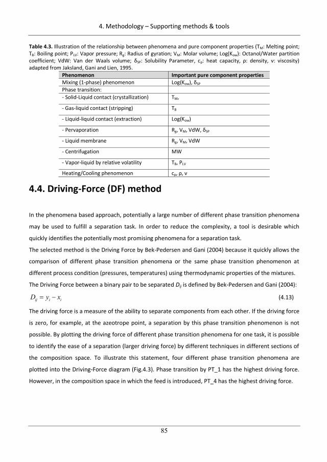
4. Methodology – Supporting methods & tools
85
Table 4.3. Illustration of the relationship between phenomena and pure component properties (TM: Melting point; TB: Boiling point; PLV: Vapor pressure; Rg: Radius of gyration; VM: Molar volume; Log(Kow): Octanol/Water partition coefficient; VdW: Van der Waals volume; SP: Solubility Parameter, cp: heat capacity, : density, : viscosity) adapted from Jaksland, Gani and Lien, 1995.
Phenomenon Important pure component properties Mixing (1-phase) phenomenon Log(Kow), SP Phase transition: - Solid-Liquid contact (crystallization) TM,
- Gas-liquid contact (stripping) TB
- Liquid-liquid contact (extraction) Log(Kow)
- Pervaporation Rg, VM, VdW, SP
- Liquid membrane Rg, VM, VdW
- Centrifugation MW
- Vapor-liquid by relative volatility TB, PLV
Heating/Cooling phenomenon cp, ,
4.4. Driving-Force (DF) method
In the phenomena based approach, potentially a large number of different phase transition phenomena
may be used to fulfill a separation task. In order to reduce the complexity, a tool is desirable which
quickly identifies the potentially most promising phenomena for a separation task.
The selected method is the Driving Force by Bek-Pedersen and Gani (2004) because it quickly allows the
comparison of different phase transition phenomena or the same phase transition phenomenon at
different process condition (pressures, temperatures) using thermodynamic properties of the mixtures.
The Driving Force between a binary pair to be separated Dij is defined by Bek-Pedersen and Gani (2004):
ij i iD y x (4.13)
The driving force is a measure of the ability to separate components from each other. If the driving force
is zero, for example, at the azeotrope point, a separation by this phase transition phenomenon is not
possible. By plotting the driving force of different phase transition phenomena for one task, it is possible
to identify the ease of a separation (larger driving force) by different techniques in different sections of
the composition space. To illustrate this statement, four different phase transition phenomena are
plotted into the Driving-Force diagram (Fig.4.3). Phase transition by PT_1 has the highest driving force.
However, in the composition space in which the feed is introduced, PT_4 has the highest driving force.
115
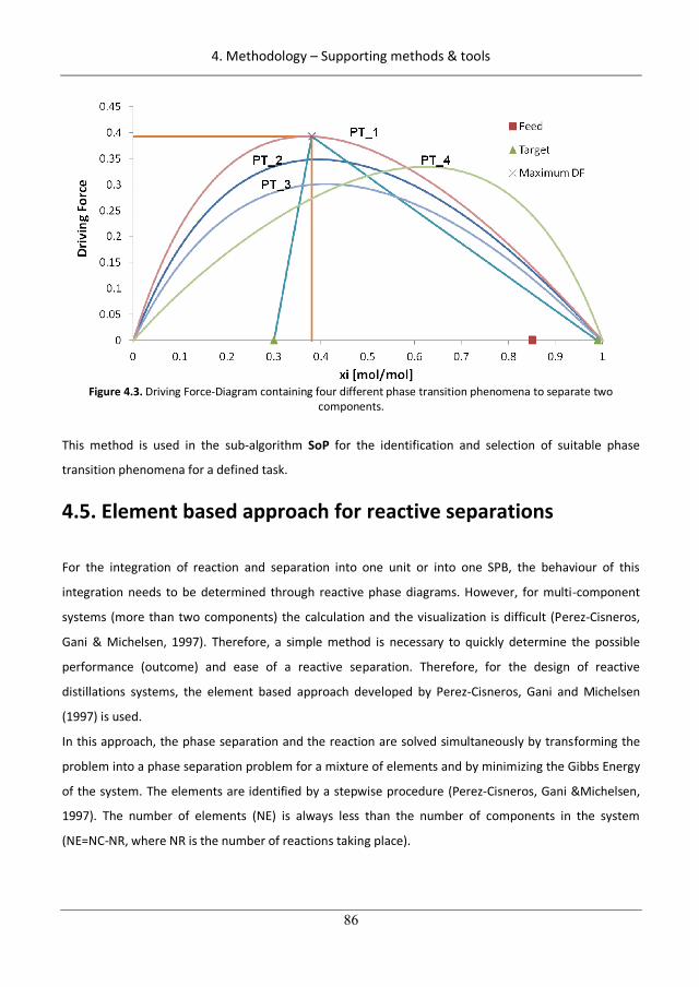
4. Methodology – Supporting methods & tools
86
Figure 4.3. Driving Force-Diagram containing four different phase transition phenomena to separate two
components.
This method is used in the sub-algorithm SoP for the identification and selection of suitable phase
transition phenomena for a defined task.
4.5. Element based approach for reactive separations
For the integration of reaction and separation into one unit or into one SPB, the behaviour of this
integration needs to be determined through reactive phase diagrams. However, for multi-component
systems (more than two components) the calculation and the visualization is difficult (Perez-Cisneros,
Gani & Michelsen, 1997). Therefore, a simple method is necessary to quickly determine the possible
performance (outcome) and ease of a reactive separation. Therefore, for the design of reactive
distillations systems, the element based approach developed by Perez-Cisneros, Gani and Michelsen
(1997) is used.
In this approach, the phase separation and the reaction are solved simultaneously by transforming the
problem into a phase separation problem for a mixture of elements and by minimizing the Gibbs Energy
of the system. The elements are identified by a stepwise procedure (Perez-Cisneros, Gani &Michelsen,
1997). The number of elements (NE) is always less than the number of components in the system
(NE=NC-NR, where NR is the number of reactions taking place).
116
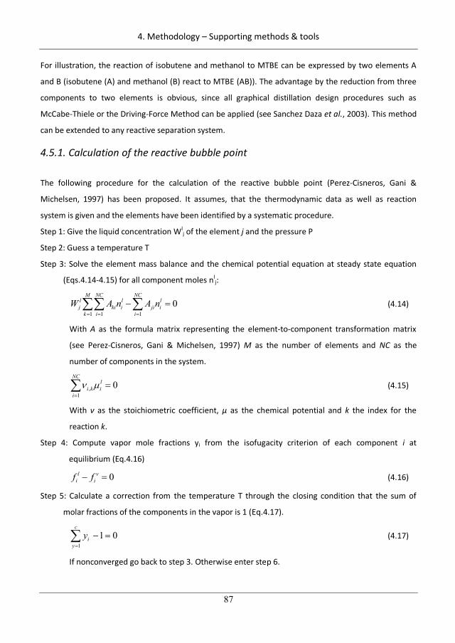
4. Methodology – Supporting methods & tools
87
For illustration, the reaction of isobutene and methanol to MTBE can be expressed by two elements A
and B (isobutene (A) and methanol (B) react to MTBE (AB)). The advantage by the reduction from three
components to two elements is obvious, since all graphical distillation design procedures such as
McCabe-Thiele or the Driving-Force Method can be applied (see Sanchez Daza et al., 2003). This method
can be extended to any reactive separation system.
4.5.1. Calculation of the reactive bubble point
The following procedure for the calculation of the reactive bubble point (Perez-Cisneros, Gani &
Michelsen, 1997) has been proposed. It assumes, that the thermodynamic data as well as reaction
system is given and the elements have been identified by a systematic procedure.
Step 1: Give the liquid concentration Wlj of the element j and the pressure P
Step 2: Guess a temperature T
Step 3: Solve the element mass balance and the chemical potential equation at steady state equation
(Eqs.4.14-4.15) for all component moles nlj:
1 1 10
M NC NCl l lj ki i ji i
k i iW A n A n (4.14)
With A as the formula matrix representing the element-to-component transformation matrix
(see Perez-Cisneros, Gani & Michelsen, 1997) M as the number of elements and NC as the
number of components in the system.
,1
0NC
li k i
i (4.15)
With as the stoichiometric coefficient, as the chemical potential and k the index for the
reaction k.
Step 4: Compute vapor mole fractions yi from the isofugacity criterion of each component i at
equilibrium (Eq.4.16)
0l vi if f (4.16)
Step 5: Calculate a correction from the temperature T through the closing condition that the sum of
molar fractions of the components in the vapor is 1 (Eq.4.17).
1
1 0c
iy
y (4.17)
If nonconverged go back to step 3. Otherwise enter step 6.
117
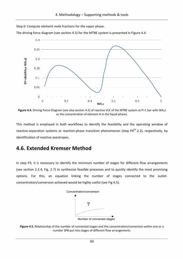
4. Methodology – Supporting methods & tools
88
Step 6: Compute element mole fractions for the vapor phase.
The driving force diagram (see section 4.5) for the MTBE system is presented in Figure 4.4.
Figure 4.4. Driving Force-Diagram (see also section 4.5) of reactive VLE of the MTBE system at P=1 bar with WA,x
as the concentration of element A in the liquid phase).
This method is employed in both workflows to identify the feasibility and the operating window of
reactive-separation systems or reaction-phase transition phenomenon (step P4SP.2.2), respectively, by
identification of reactive azeotropes.
4.6. Extended Kremser Method
In step P3, it is necessary to identify the minimum number of stages for different flow arrangements
(see section 2.2.4, Fig. 2.7) to synthesize feasible processes and to quickly identify the most promising
options. For this, an equation linking the number of stages connected to the outlet-
concentration/conversion achieved would be highly useful (see Fig 4.5).
Number of connected stages
Concentration/conversion
?
Figure 4.5. Relationship of the number of connected stages and the concentration/conversion within one or a
number SPB put into stages of different flow arrangements.
118
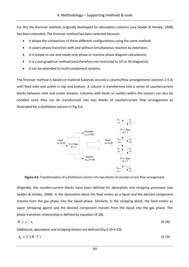
4. Methodology – Supporting methods & tools
89
For this the Kremser method, originally developed for absorption columns (see Seader & Henley, 1998)
has been extended. The Kremser method has been selected because:
it allows the comparison of three different configurations using the same method;
it covers phase-transition with and without simultaneous reaction by extension;
it is simple to use and needs only phase or reactive phase diagram calculations;
it is a non graphical method (and therefore not restricted to 2D or 3D diagrams);
it can be extended to multi-component systems.
The Kremser method is based on material balances around a column/flow arrangements (section 2.4.4)
with feed inlet and outlet in top and bottom. A column is transformed into a series of countercurrent
blocks between inlet and outlet streams. Columns with feeds or outlets within the column can also be
handled since they can be transformed into two blocks of countercurrent flow arrangement as
illustrated for a distillation column in Fig.4.6.
P=1.3barN = ?
FeedxA=0.25
DistillatexD,A=0.95
BottomxB,W=0.98
L0,x0
LN,xN
VN+1,yN+1
V0,y0
L0,x0
LN,xN
VN+1,yN+1
V0,y0
FeedxA=0.25
P=1.3barN = ?
P=1.3barN = ?
Figure 4.6. Transformation of a distillation column into two blocks of countercurrent flow arrangement.
Originally, the counter-current blocks have been defined for absorption and stripping processes (see
Seader & Henley, 1998). In the absorption block the feed enters as a liquid and the desired component
transits from the gas phase into the liquid phase. Similarly, in the stripping block, the feed enters as
vapor (stripping agent) and the desired component transits from the liquid into the gas phase. The
phase transition relationship is defined by equation (4.18).
/i iK y x (4.18)
Additional, absorption and stripping factors are defined (Eq.4.19-4.20).
/( )EA L K V (4.19)
119
4. Methodology – Supporting methods & tools
90
( ) / 1/E ES K V L A (4.20)
Absorption and stripping factors (Eqs. 4.19-4.20) have been adapted for different phase transition
phenomena which have been listed in Table 3.5. In cases of simultaneous reaction and phase transition
phenomena, the element-based approach in section 4.5 is used to generate reactive phase diagrams to
calculate the necessary K-values.
The recovery of one countercurrent block (see Fig 4.6) is defined as:
01
11
yyyy
n
n .
(4.21)
With 0y as the vapor concentration in equilibrium to the entering liquid.
Through material balances in each stage from the top to the bottom, the stages are linked through inlet
and outlets. The recovery can be derived for co-current, cross-current and counter-current flow
arrangements by a simple equation using the absorption/stripping factor respectively (see equations
4.32-4.34). The complete derivation is given elsewhere (Seader & Henley, 1998).
Co-current:
111 EA
(4.22)
Cross-current:
111 n
EA N (4.23)
Counter-current:
11
E
E
ALnn
Ln A (4.24)
The application of the extended Kremser method is illustrated in appendix A.4 comparing the method to
the McCabe-Thiele method.
4.6.1. Derivation of the relationship between DF and Rmin to be used for the
determination of the minimum ratio R=L/V
For the application of the extended Kremser method a reliable method giving a good estimate for the
ratio of the two phase flows (L/V) is necessary. Here, the driving force method is used to find good
initial estimates for a low energy consumption corresponding to Rmin. For simplification, it is shown
120
4. Methodology – Supporting methods & tools
91
here for the phase transition phenomena by relative volatility. However, the results can be generalized
for all types of phase transition phenomena or integrated reactive phase transition phenomena.
Two sections may exist in the arrangement. An absorption section in which the feed is vaporized and
moves upwards and a stripping section on which the feed is liquefied and moves downwards (see Fig.
4.6).
Absorption section:
Feed is vaporized ( in Feedy x )
A mass balance around the absorption section gives:
/ / Dy L V x D V x (4.25)
Transformation of the distillate flowrate D:
/ ( ) / Dy L V x V L V x (4.26)
Assuming that V and L are constant, V and F equal and defining a ratio of flows R with
/R L V (4.27)
gives for equation (4.26):
( )D Dy R x x x (4.28)
Inserting this equation into the definition for the driving force (equation (4.13)) gives:
( ) /( )D Dy R y x x x (4.29)
In which the x is the equilibrium concentration to y.
Stripping section:
Feed is liquid ( in Feedx x )
A mass balance around the stripping section gives:
/ / By L V x B V x (4.30)
Transformation of the bottom flowrate B:
/ ( ) / By L V x L V V x (4.31)
Assuming that V and L are constant, V and F equal and defining a ratio of flows R with
/R L V (4.32)
gives for equation (4.32):
( )B By R x x x (4.33)
Inserting this equation into the definition for the driving force (equation (4.13) gives:
( ) /( )B By R y x x x (4.34)
121
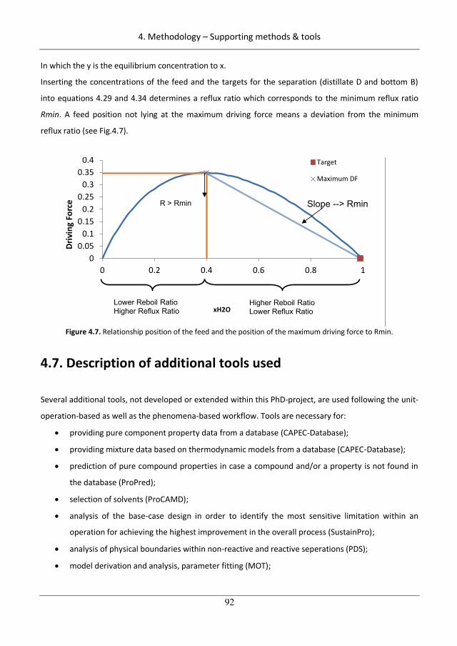
4. Methodology – Supporting methods & tools
92
In which the y is the equilibrium concentration to x.
Inserting the concentrations of the feed and the targets for the separation (distillate D and bottom B)
into equations 4.29 and 4.34 determines a reflux ratio which corresponds to the minimum reflux ratio
Rmin. A feed position not lying at the maximum driving force means a deviation from the minimum
reflux ratio (see Fig.4.7).
00.05
0.10.15
0.20.25
0.30.35
0.4
0 0.2 0.4 0.6 0.8 1
Driv
ing
Forc
e
xH2O
Target
Maximum DF
Slope --> Rmin
Lower Reboil RatioHigher Reflux Ratio
Higher Reboil RatioLower Reflux Ratio
R > Rmin
Figure 4.7. Relationship position of the feed and the position of the maximum driving force to Rmin.
4.7. Description of additional tools used
Several additional tools, not developed or extended within this PhD-project, are used following the unit-
operation-based as well as the phenomena-based workflow. Tools are necessary for:
providing pure component property data from a database (CAPEC-Database);
providing mixture data based on thermodynamic models from a database (CAPEC-Database);
prediction of pure compound properties in case a compound and/or a property is not found in
the database (ProPred);
selection of solvents (ProCAMD);
analysis of the base-case design in order to identify the most sensitive limitation within an
operation for achieving the highest improvement in the overall process (SustainPro);
analysis of physical boundaries within non-reactive and reactive seperations (PDS);
model derivation and analysis, parameter fitting (MOT);
122
4. Methodology – Supporting methods & tools
93
model simulation, optimization and validation (MOT, ICASSim, Pro\II);
Some of these tools are available in ICAS, an Integrated Computer Aided System, developed in CAPEC, a
research center at the Technical University of Denmark, DTU such as: CAPEC-Database, ProPred,
ProCAMD, SustainPro, PDS, MOT, ICASSim. Additionally, a commercial program is used which is Pro\II
(Pro\II, 2011).
CAPEC-Database: This tool is managing the various databases within ICAS such as component and the
reaction database. This tool is used in steps 2 and 3 for identification of pure component as well as
mixture properties (based on the use of thermodynamic models).
ProPred: ProPred is for pure component property prediction. In this tool, properties of pure compounds
are predicted from their molecular structure such as boiling point, melting point, octanol-water partition
coefficient. Several methods for the prediction are used such as the Marrero-Gani approach (see
Marrero & Gani, 2001). This tool is necessary in the sub-algorithm APCP to analyze the given process
based on pure component properties whenever they are not found in the component database.
ProCAMD: In ProCAMD, the computer aided molecular design approach is implemented (see Harper &
Gani, 2000) in which based on a set of given molecular groups a number of feasible components are
synthesized to match a number of specified target properties. Within this PhD-project, this tool is used
to identify solvents in the sub-algorithm SoP (if specified) in case of identified liquid-liquid phase
transition phenomena.
SustainPro: In this tool, the method from Carvalho et al. (2008) is implemented. The process flowsheet
of the base-case design is decomposed into a set of process graphs. For each of these process graphs,
mass and energy indicators such as material-value-added or energy and waste costs are calculated
needing information about costs/prices of input and output mass/energy. Based on these indicators
limitations/bottlenecks are identified for improving the sustainability of the process. In this PhD-project,
this tool is used in the sub-algorithm MBS for analysis of the base-case design.
PDS: PDS stands for process design studio. This tool is used for the analysis and the design of distillation
columns as well as reactive distillation columns using the element approach (see section 4.5). In this
project, this tool is used in the sub-algorithm OPW for identification of process boundaries (vapor-liquid
phase diagrams, reactive and non-reactive azeotropes).
MOT: MOT stands for Modelling Testbed. In this tool, all necessary sub-tools for efficient and systematic
model development, analysis, identification and application are integrated. In this project, it is used in
steps U3-6 and P4-6 for model derivation and analysis, parameter fitting, simulation and optimization.
123
4. Methodology – Supporting methods & tools
94
ICASSim: ICASSim is a steady-state rigorous simulation tool to perform mass and energy balances in a
process. In ICASSim, steady state simulation models for a number of predefined unit-operations are
available. Specific models, derived in MOT can also be integrated. In this project, ICASSim is used for
validation of the results in step 6.4.
Pro\II: Pro\II is a commercial process engineering suite (Pro\II, 2011) from Invensys SIMSCI Esscor to
perform mass and energy balance calculations for a specified process. In this PhD-project, it is used for
validation of the obtained results by rigorous simulation in step 6.4.
124
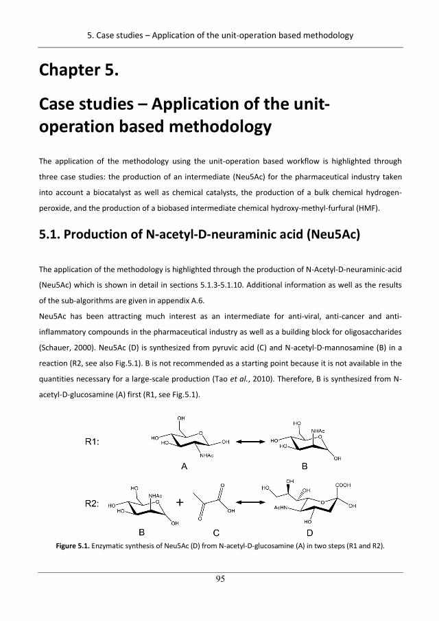
5. Case studies – Application of the unit-operation based methodology
95
Chapter 5.
Case studies – Application of the unit-operation based methodology
The application of the methodology using the unit-operation based workflow is highlighted through
three case studies: the production of an intermediate (Neu5Ac) for the pharmaceutical industry taken
into account a biocatalyst as well as chemical catalysts, the production of a bulk chemical hydrogen-
peroxide, and the production of a biobased intermediate chemical hydroxy-methyl-furfural (HMF).
5.1. Production of N-acetyl-D-neuraminic acid (Neu5Ac)
The application of the methodology is highlighted through the production of N-Acetyl-D-neuraminic-acid
(Neu5Ac) which is shown in detail in sections 5.1.3-5.1.10. Additional information as well as the results
of the sub-algorithms are given in appendix A.6.
Neu5Ac has been attracting much interest as an intermediate for anti-viral, anti-cancer and anti-
inflammatory compounds in the pharmaceutical industry as well as a building block for oligosaccharides
(Schauer, 2000). Neu5Ac (D) is synthesized from pyruvic acid (C) and N-acetyl-D-mannosamine (B) in a
reaction (R2, see also Fig.5.1). B is not recommended as a starting point because it is not available in the
quantities necessary for a large-scale production (Tao et al., 2010). Therefore, B is synthesized from N-
acetyl-D-glucosamine (A) first (R1, see Fig.5.1).
Figure 5.1. Enzymatic synthesis of Neu5Ac (D) from N-acetyl-D-glucosamine (A) in two steps (R1 and R2).
125
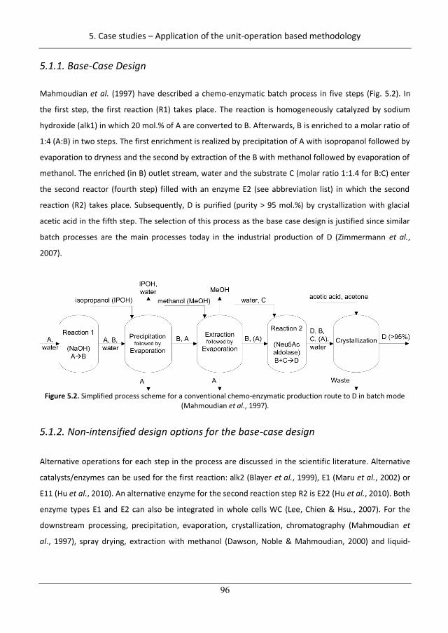
5. Case studies – Application of the unit-operation based methodology
96
5.1.1. Base-Case Design
Mahmoudian et al. (1997) have described a chemo-enzymatic batch process in five steps (Fig. 5.2). In
the first step, the first reaction (R1) takes place. The reaction is homogeneously catalyzed by sodium
hydroxide (alk1) in which 20 mol.% of A are converted to B. Afterwards, B is enriched to a molar ratio of
1:4 (A:B) in two steps. The first enrichment is realized by precipitation of A with isopropanol followed by
evaporation to dryness and the second by extraction of the B with methanol followed by evaporation of
methanol. The enriched (in B) outlet stream, water and the substrate C (molar ratio 1:1.4 for B:C) enter
the second reactor (fourth step) filled with an enzyme E2 (see abbreviation list) in which the second
reaction (R2) takes place. Subsequently, D is purified (purity > 95 mol.%) by crystallization with glacial
acetic acid in the fifth step. The selection of this process as the base case design is justified since similar
batch processes are the main processes today in the industrial production of D (Zimmermann et al.,
2007).
Figure 5.2. Simplified process scheme for a conventional chemo-enzymatic production route to D in batch mode
(Mahmoudian et al., 1997).
5.1.2. Non-intensified design options for the base-case design
Alternative operations for each step in the process are discussed in the scientific literature. Alternative
catalysts/enzymes can be used for the first reaction: alk2 (Blayer et al., 1999), E1 (Maru et al., 2002) or
E11 (Hu et al., 2010). An alternative enzyme for the second reaction step R2 is E22 (Hu et al., 2010). Both
enzyme types E1 and E2 can also be integrated in whole cells WC (Lee, Chien & Hsu., 2007). For the
downstream processing, precipitation, evaporation, crystallization, chromatography (Mahmoudian et
al., 1997), spray drying, extraction with methanol (Dawson, Noble & Mahmoudian, 2000) and liquid-
126
5. Case studies – Application of the unit-operation based methodology
97
liquid extraction with a reactive solvent (Zimmermann et al., 2008) can be used. All these non-
intensified options will also be considered.
5.1.3. Step 1: Define problem
Step 1.1: The objective is to achieve PI (unit-operation) for the maximization of the ratio of the space-
time-yield of the process P against the space-time-yield of base case design P,0 as FObj:
,0max / , , ,Obj P P jF f Y X d (5.1)
The space-time-yield is defined as the product produced per day and volume (Eq.5.2):
0/ /P D Rm V t (5.2)
Step 1.2: The design scenario is to develop a new design of the whole process. The process scenario is
batch because even though the enzymes are expensive, they are stable enough to run in more
than one batch operation (Blayer et al., 1999). However, the long time stability of the enzymes is
not satisfactory for a continuous operation yet (Hu et al.. 2010).
Step 1.3: The product D is produced from the raw materials A and C. All raw materials are pure and the
purity of the product D is defined to be at least 95% (molar basis). Water is used as the solvent.
The pressure is assumed to be 1 bar.
Step 1.4: Waste, efficiency, energy consumption, simplification, time yield of the reaction, the product
yield of the whole process.
Step 1.5: The maturity of the process is defined to be “high”.
Step 1.6: Translate and PM into logical (Eq.2.2), structural (Eq.2.3), operational constraints (Eq.2.5)
and/or performance criteria (Eq.2.6):
Step 1.6.1: All rules have been applied to gather a set of logical constraints (Eq.2.2). The detailed
results are listed in Table 5.1.
Step 1.6.2: Four PI metrics have been translated to six structural constraints (see Table 5.1).
Step 1.6.3: The result of the translation into operational constraints (Eq.2.5) and the PI screening
criterion (Eq.2.6) is given in Table 5.1. The time-yield of the reaction R is defined by equation
(5.3) and the product-yield by equation (5.4).
RADR tmm // . (5.3)
%100/ AD nn (5.4)
Step 1.7: A base case design exists, step A2 is entered (rule 1.9).
127
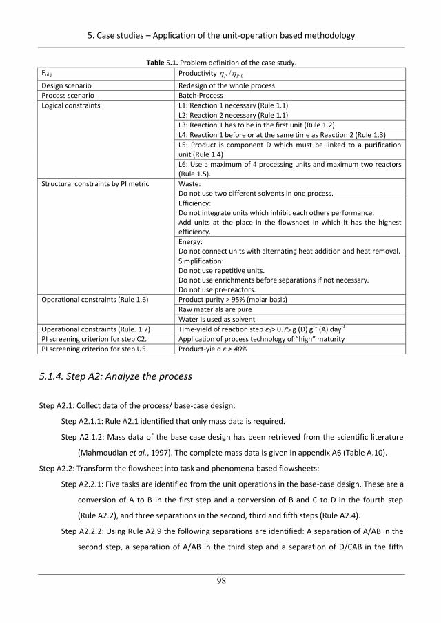
5. Case studies – Application of the unit-operation based methodology
98
Table 5.1. Problem definition of the case study. Fobj Productivity ,0/P P Design scenario Redesign of the whole process Process scenario Batch-Process Logical constraints L1: Reaction 1 necessary (Rule 1.1)
L2: Reaction 2 necessary (Rule 1.1) L3: Reaction 1 has to be in the first unit (Rule 1.2) L4: Reaction 1 before or at the same time as Reaction 2 (Rule 1.3) L5: Product is component D which must be linked to a purification unit (Rule 1.4) L6: Use a maximum of 4 processing units and maximum two reactors (Rule 1.5).
Structural constraints by PI metric Waste: Do not use two different solvents in one process. Efficiency: Do not integrate units which inhibit each others performance. Add units at the place in the flowsheet in which it has the highest efficiency. Energy: Do not connect units with alternating heat addition and heat removal. Simplification: Do not use repetitive units. Do not use enrichments before separations if not necessary. Do not use pre-reactors.
Operational constraints (Rule 1.6) Product purity > 95% (molar basis) Raw materials are pure Water is used as solvent
Operational constraints (Rule. 1.7) Time-yield of reaction step R> 0.75 g (D) g-1 (A) day-1 PI screening criterion for step C2. Application of process technology of “high” maturity PI screening criterion for step U5 Product-yield > 40%
5.1.4. Step A2: Analyze the process
Step A2.1: Collect data of the process/ base-case design:
Step A2.1.1: Rule A2.1 identified that only mass data is required.
Step A2.1.2: Mass data of the base case design has been retrieved from the scientific literature
(Mahmoudian et al., 1997). The complete mass data is given in appendix A6 (Table A.10).
Step A2.2: Transform the flowsheet into task and phenomena-based flowsheets:
Step A2.2.1: Five tasks are identified from the unit operations in the base-case design. These are a
conversion of A to B in the first step and a conversion of B and C to D in the fourth step
(Rule A2.2), and three separations in the second, third and fifth steps (Rule A2.4).
Step A2.2.2: Using Rule A2.9 the following separations are identified: A separation of A/AB in the
second step, a separation of A/AB in the third step and a separation of D/CAB in the fifth
128
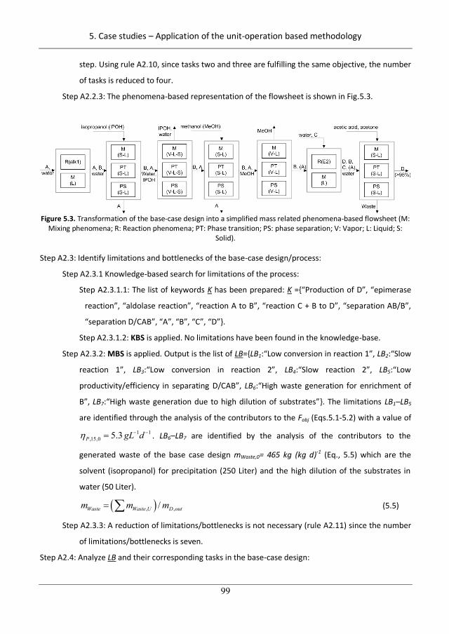
5. Case studies – Application of the unit-operation based methodology
99
step. Using rule A2.10, since tasks two and three are fulfilling the same objective, the number
of tasks is reduced to four.
Step A2.2.3: The phenomena-based representation of the flowsheet is shown in Fig.5.3.
Figure 5.3. Transformation of the base-case design into a simplified mass related phenomena-based flowsheet (M:
Mixing phenomena; R: Reaction phenomena; PT: Phase transition; PS: phase separation; V: Vapor; L: Liquid; S: Solid).
Step A2.3: Identify limitations and bottlenecks of the base-case design/process:
Step A2.3.1 Knowledge-based search for limitations of the process:
Step A2.3.1.1: The list of keywords K has been prepared: K ={“Production of D”, “epimerase
reaction”, “aldolase reaction”, “reaction A to B”, “reaction C + B to D”, “separation AB/B”,
“separation D/CAB”, “A”, “B”, “C”, “D”}.
Step A2.3.1.2: KBS is applied. No limitations have been found in the knowledge-base.
Step A2.3.2: MBS is applied. Output is the list of LB={LB1:“Low conversion in reaction 1”, LB2:“Slow
reaction 1”, LB3:“Low conversion in reaction 2”, LB4:“Slow reaction 2”, LB5:“Low
productivity/efficiency in separating D/CAB”, LB6:“High waste generation for enrichment of
B”, LB7:“High waste generation due to high dilution of substrates”}. The limitations LB1–LB5
are identified through the analysis of the contributors to the Fobj (Eqs.5.1-5.2) with a value of 1 1
,15,0 5.3P gL d . LB6–LB7 are identified by the analysis of the contributors to the
generated waste of the base case design mWaste,0= 465 kg (kg d)-1 (Eq., 5.5) which are the
solvent (isopropanol) for precipitation (250 Liter) and the high dilution of the substrates in
water (50 Liter).
, ,/Waste Waste U D outm m m (5.5)
Step A2.3.3: A reduction of limitations/bottlenecks is not necessary (rule A2.11) since the number
of limitations/bottlenecks is seven.
Step A2.4: Analyze LB and their corresponding tasks in the base-case design:
129
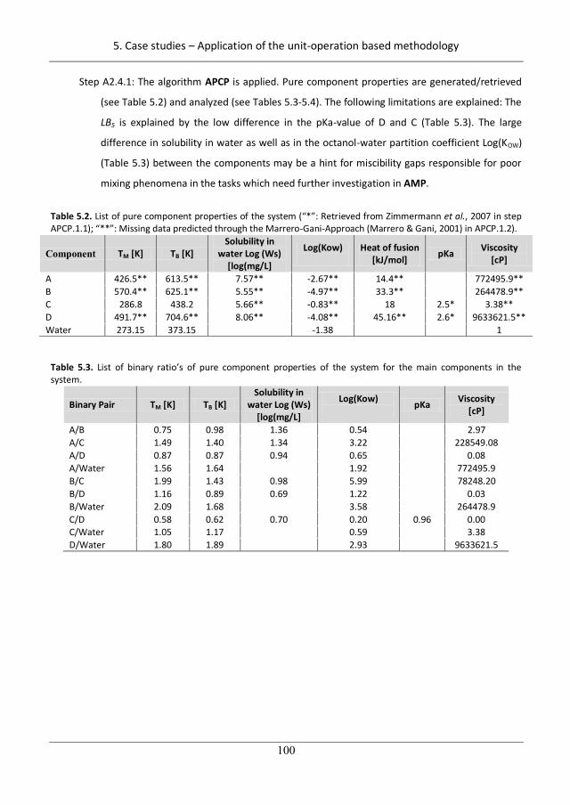
5. Case studies – Application of the unit-operation based methodology
100
Step A2.4.1: The algorithm APCP is applied. Pure component properties are generated/retrieved
(see Table 5.2) and analyzed (see Tables 5.3-5.4). The following limitations are explained: The
LB5 is explained by the low difference in the pKa-value of D and C (Table 5.3). The large
difference in solubility in water as well as in the octanol-water partition coefficient Log(KOW)
(Table 5.3) between the components may be a hint for miscibility gaps responsible for poor
mixing phenomena in the tasks which need further investigation in AMP.
Table 5.2. List of pure component properties of the system (“*”: Retrieved from Zimmermann et al., 2007 in step APCP.1.1); “**”: Missing data predicted through the Marrero-Gani-Approach (Marrero & Gani, 2001) in APCP.1.2).
Component TM [K] TB [K] Solubility in
water Log (Ws) [log(mg/L]
Log(Kow)
Heat of fusion [kJ/mol] pKa Viscosity
[cP]
A 426.5** 613.5** 7.57** -2.67** 14.4** 772495.9** B 570.4** 625.1** 5.55** -4.97** 33.3** 264478.9** C 286.8 438.2 5.66** -0.83** 18 2.5* 3.38** D 491.7** 704.6** 8.06** -4.08** 45.16** 2.6* 9633621.5** Water 273.15 373.15 -1.38 1
Table 5.3. List of binary ratio’s of pure component properties of the system for the main components in the system.
Binary Pair TM [K] TB [K] Solubility in
water Log (Ws) [log(mg/L]
Log(Kow) pKa Viscosity
[cP]
A/B 0.75 0.98 1.36 0.54 2.97 A/C 1.49 1.40 1.34 3.22 228549.08 A/D 0.87 0.87 0.94 0.65 0.08 A/Water 1.56 1.64 1.92 772495.9 B/C 1.99 1.43 0.98 5.99 78248.20 B/D 1.16 0.89 0.69 1.22 0.03 B/Water 2.09 1.68 3.58 264478.9 C/D 0.58 0.62 0.70 0.20 0.96 0.00 C/Water 1.05 1.17 0.59 3.38 D/Water 1.80 1.89 2.93 9633621.5
130
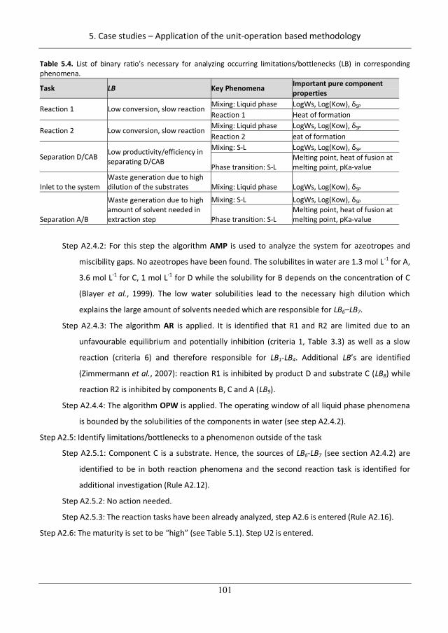
5. Case studies – Application of the unit-operation based methodology
101
Table 5.4. List of binary ratio’s necessary for analyzing occurring limitations/bottlenecks (LB) in corresponding phenomena.
Task LB Key Phenomena Important pure component properties
Reaction 1 Low conversion, slow reaction Mixing: Liquid phase LogWs, Log(Kow), SP Reaction 1 Heat of formation
Reaction 2 Low conversion, slow reaction Mixing: Liquid phase LogWs, Log(Kow), SP Reaction 2 eat of formation
Separation D/CAB Low productivity/efficiency in separating D/CAB
Mixing: S-L LogWs, Log(Kow), SP
Phase transition: S-L Melting point, heat of fusion at melting point, pKa-value
Inlet to the system Waste generation due to high dilution of the substrates Mixing: Liquid phase LogWs, Log(Kow), SP
Separation A/B
Waste generation due to high amount of solvent needed in extraction step
Mixing: S-L LogWs, Log(Kow), SP
Phase transition: S-L Melting point, heat of fusion at melting point, pKa-value
Step A2.4.2: For this step the algorithm AMP is used to analyze the system for azeotropes and
miscibility gaps. No azeotropes have been found. The solubilites in water are 1.3 mol L-1 for A,
3.6 mol L-1 for C, 1 mol L-1 for D while the solubility for B depends on the concentration of C
(Blayer et al., 1999). The low water solubilities lead to the necessary high dilution which
explains the large amount of solvents needed which are responsible for LB6–LB7.
Step A2.4.3: The algorithm AR is applied. It is identified that R1 and R2 are limited due to an
unfavourable equilibrium and potentially inhibition (criteria 1, Table 3.3) as well as a slow
reaction (criteria 6) and therefore responsible for LB1-LB4. Additional LB’s are identified
(Zimmermann et al., 2007): reaction R1 is inhibited by product D and substrate C (LB8) while
reaction R2 is inhibited by components B, C and A (LB9).
Step A2.4.4: The algorithm OPW is applied. The operating window of all liquid phase phenomena
is bounded by the solubilities of the components in water (see step A2.4.2).
Step A2.5: Identify limitations/bottlenecks to a phenomenon outside of the task
Step A2.5.1: Component C is a substrate. Hence, the sources of LB6-LB7 (see section A2.4.2) are
identified to be in both reaction phenomena and the second reaction task is identified for
additional investigation (Rule A2.12).
Step A2.5.2: No action needed.
Step A2.5.3: The reaction tasks have been already analyzed, step A2.6 is entered (Rule A2.16).
Step A2.6: The maturity is set to be “high” (see Table 5.1). Step U2 is entered.
131
5. Case studies – Application of the unit-operation based methodology
102
5.1.5. Step U2: Collect PI equipment
Step U2.1 Collect potential PI equipment:
Step U2.1.1: The list of keywords contains KPI={(1):“Unfavourable equilibrium in reaction 1”, (2):
“Substrate and product inhibition in reaction 1”, (3):“Slow reaction 1”, (4):“ Unfavourable
equilibrium in reaction 2”, (5): Substrate and product inhibition in reaction 2”, (6):“Slow
reaction 2”, (7): “epimerase reaction”, (8): “aldolase reaction”}.
Step U2.1.2: In total 24 PI equipment are retrieved from the knowledge-base (see Table A.11 in
appendix A6). Also included in this table are the keywords responsible for the selection. Note:
The reaction task can be single reactions or multiple reactions. For multiple reactions (R1 and
R2 together), all combinations of catalysts/enzymes for each reaction R1 and R2 in a single
unit are considered. Therefore, 15 different reactor combinations are potentially possible.
Hence, a reactive-extraction can be run in 15 configurations. That gives in total 360 items of
PI equipment and 13 items of non-intensified equipment (see section 5.1.2) in the search
space.
Step U2.2: Pre-screen candidate PI equipment for feasibility and maturity:
Step U2.2.1-U2.2.3: The result of the pre-screening for feasibility is presented in Table A.11 in
appendix A.6. In total, 91 intensified and 13 non-intensified options remain in the search
space.
Step U2.2.4: After screening for maturity (Rule U2.4), the remaining equipment are a one-pot-
reactor with 5 different catalysts/combinations (E1/E2, E11/E22, WC, alk1/E2, alk1/E22), 5
single reactors (alk1, E1, E11, E2, E22), reactive-extraction including all 10 remaining reactor
configurations and 7 non-PI separations (precipitation, evaporation, crystallization,
chromatography, spray-dryer, extraction with methanol, extraction with reactive solvent). A
known solvent has been selected which is PBA/ TOMAC (Zimmermann et al., 2008) (Rule
U2.2). That gives in total 27 items of equipment.
Step U2.3: Identify sub-problems:
Step U2.3.1: The number of sub-problems is identified to be 1 (Rule U2.4).
Step U2.3.2: All equipment from step 2.2.4 are added to SP=1.
Step U2.3.3: Step U3SP=1 is entered for sub-problem 1.
132
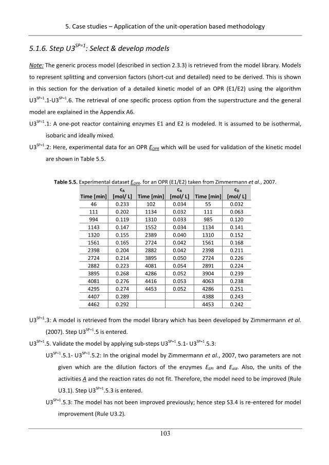
5. Case studies – Application of the unit-operation based methodology
103
5.1.6. Step U3SP=1: Select & develop models
Note: The generic process model (described in section 2.3.3) is retrieved from the model library. Models
to represent splitting and conversion factors (short-cut and detailed) need to be derived. This is shown
in this section for the derivation of a detailed kinetic model of an OPR (E1/E2) using the algorithm
U3SP=1.1-U3SP=1.6. The retrieval of one specific process option from the superstructure and the general
model are explained in the Appendix A6.
U3SP=1.1: A one-pot reactor containing enzymes E1 and E2 is modeled. It is assumed to be isothermal,
isobaric and ideally mixed.
U3SP=1.2: Here, experimental data for an OPR EOPR which will be used for validation of the kinetic model
are shown in Table 5.5.
Table 5.5. Experimental dataset EOPR. for an OPR (E1/E2) taken from Zimmermann et al., 2007.
Time [min] cA
[mol/ L] Time [min] cA
[mol/ L] Time [min] cD
[mol/ L] 46 0.233 102 0.034 55 0.032
111 0.202 1134 0.032 111 0.063 994 0.119 1310 0.033 985 0.120
1143 0.147 1552 0.034 1134 0.141 1320 0.155 2389 0.040 1310 0.152 1561 0.165 2724 0.042 1561 0.168 2398 0.204 2882 0.042 2398 0.211 2724 0.214 3895 0.050 2724 0.226 2882 0.223 4081 0.054 2891 0.224 3895 0.268 4286 0.052 3904 0.239 4081 0.276 4416 0.053 4063 0.238 4295 0.274 4453 0.052 4286 0.251 4407 0.289 4388 0.243 4462 0.292 4453 0.242
U3SP=1.3: A model is retrieved from the model library which has been developed by Zimmermann et al.
(2007). Step U3SP=1.5 is entered.
U3SP=1.5. Validate the model by applying sub-steps U3SP=1.5.1- U3SP=1.5.3:
U3SP=1.5.1- U3SP=1.5.2: In the original model by Zimmermann et al., 2007, two parameters are not
given which are the dilution factors of the enzymes EEPI and Eald. Also, the units of the
activities A and the reaction rates do not fit. Therefore, the model need to be improved (Rule
U3.1). Step U3SP=1.5.3 is entered.
U3SP=1.5.3: The model has not been improved previously; hence step S3.4 is re-entered for model
improvement (Rule U3.2).
133
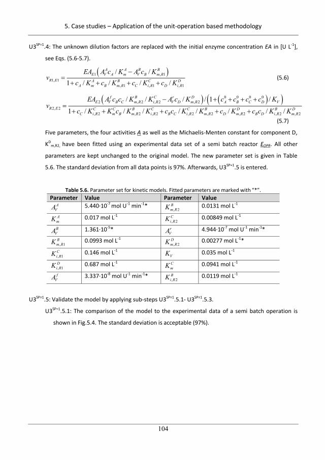
5. Case studies – Application of the unit-operation based methodology
104
U3SP=1.4: The unknown dilution factors are replaced with the initial enzyme concentration EA in [U L-1],
see Eqs. (5.6-5.7).
1 , 11, 1
, 1 , 1 , 1
/ /1 / / / /
A A B BE V A m V B m R
R E A B C DA m B m R C i R D i R
EA A c K A c Kv
c K c K c K c K (5.6)
0 0 0 02 , 2 , 2 , 2
2, 2, 2 , 2 , 2 , 2 , 2 , 2 , 2 , 2
/ / / / 1 /
1 / / / / / / / /
f B C r DE V B C m R i R V D m R A B C D V
R E C C B C C B D B DC i R m B m R i R B C i R m R D m R B D i R m R
EA A c c K K A c K c c c c Kv
c K K c K K c c K K c K c c K K (5.7)
Five parameters, the four activities A as well as the Michaelis-Menten constant for component D,
KDm,R2, have been fitted using an experimental data set of a semi batch reactor EOPR. All other
parameters are kept unchanged to the original model. The new parameter set is given in Table
5.6. The standard deviation from all data points is 97%. Afterwards, U3SP=1.5 is entered.
Table 5.6. Parameter set for kinetic models. Fitted parameters are marked with “*”. Parameter Value Parameter Value
AVA 5.440·10-7 mol U-1 min-1* B
RmK 2, 0.0131 mol L-1
AmK 0.017 mol L-1 C
RiK 2, 0.00849 mol L-1
BVA 1.361·10-5* r
VA 4.944·10-7 mol U-1 min-1* B
RmK 1, 0.0993 mol L-1 DRmK 2, 0.00277 mol L-1*
CRiK 1, 0.146 mol L-1
VK 0.035 mol L-1 DRiK 1, 0.687 mol L-1 C
mK 0.0941 mol L-1
fVA 3.337·10-8 mol U-1 min-1* B
RiK 2, 0.0119 mol L-1
U3SP=1.5: Validate the model by applying sub-steps U3SP=1.5.1- U3SP=1.5.3.
U3SP=1.5.1: The comparison of the model to the experimental data of a semi batch operation is
shown in Fig.5.4. The standard deviation is acceptable (97%).
134
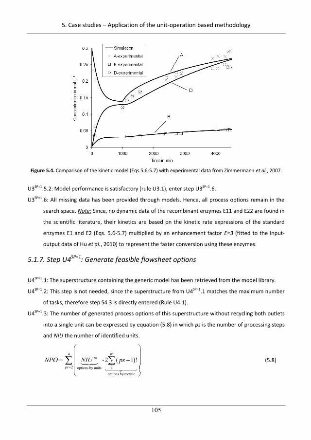
5. Case studies – Application of the unit-operation based methodology
105
Figure 5.4. Comparison of the kinetic model (Eqs.5.6-5.7) with experimental data from Zimmermann et al., 2007.
U3SP=1.5.2: Model performance is satisfactory (rule U3.1), enter step U3SP=1.6.
U3SP=1.6: All missing data has been provided through models. Hence, all process options remain in the
search space. Note: Since, no dynamic data of the recombinant enzymes E11 and E22 are found in
the scientific literature, their kinetics are based on the kinetic rate expressions of the standard
enzymes E1 and E2 (Eqs. 5.6-5.7) multiplied by an enhancement factor E=3 (fitted to the input-
output data of Hu et al., 2010) to represent the faster conversion using these enzymes.
5.1.7. Step U4SP=1: Generate feasible flowsheet options
U4SP=1.1: The superstructure containing the generic model has been retrieved from the model library.
U4SP=1.2: This step is not needed, since the superstructure from U4SP=1.1 matches the maximum number
of tasks, therefore step S4.3 is directly entered (Rule U4.1).
U4SP=1.3: The number of generated process options of this superstructure without recycling both outlets
into a single unit can be expressed by equation (5.8) in which ps is the number of processing steps
and NIU the number of identified units.
4
2 2options by unitsoptions by recycle
2 ( 1)!ps
ps
psNPO NIU psNIU 2psNIU 2p
22
(5.8)
135
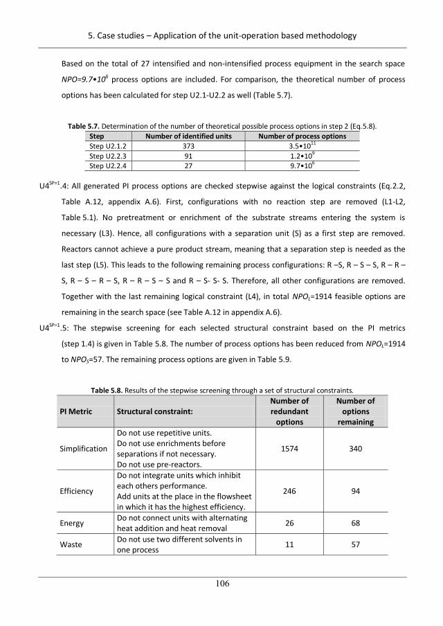
5. Case studies – Application of the unit-operation based methodology
106
Based on the total of 27 intensified and non-intensified process equipment in the search space
NPO=9.7•106 process options are included. For comparison, the theoretical number of process
options has been calculated for step U2.1-U2.2 as well (Table 5.7).
Table 5.7. Determination of the number of theoretical possible process options in step 2 (Eq.5.8). Step Number of identified units Number of process options Step U2.1.2 373 3.5•1011 Step U2.2.3 91 1.2•109 Step U2.2.4 27 9.7•106
U4SP=1.4: All generated PI process options are checked stepwise against the logical constraints (Eq.2.2,
Table A.12, appendix A.6). First, configurations with no reaction step are removed (L1-L2,
Table 5.1). No pretreatment or enrichment of the substrate streams entering the system is
necessary (L3). Hence, all configurations with a separation unit (S) as a first step are removed.
Reactors cannot achieve a pure product stream, meaning that a separation step is needed as the
last step (L5). This leads to the following remaining process configurations: R –S, R – S – S, R – R –
S, R – S – R – S, R – R – S – S and R – S- S- S. Therefore, all other configurations are removed.
Together with the last remaining logical constraint (L4), in total NPOL=1914 feasible options are
remaining in the search space (see Table A.12 in appendix A.6).
U4SP=1.5: The stepwise screening for each selected structural constraint based on the PI metrics
(step 1.4) is given in Table 5.8. The number of process options has been reduced from NPOL=1914
to NPOS=57. The remaining process options are given in Table 5.9.
Table 5.8. Results of the stepwise screening through a set of structural constraints.
PI Metric Structural constraint: Number of redundant
options
Number of options
remaining
Simplification
Do not use repetitive units. Do not use enrichments before separations if not necessary. Do not use pre-reactors.
1574 340
Efficiency
Do not integrate units which inhibit each others performance. Add units at the place in the flowsheet in which it has the highest efficiency.
246 94
Energy Do not connect units with alternating heat addition and heat removal 26 68
Waste Do not use two different solvents in one process 11 57
136
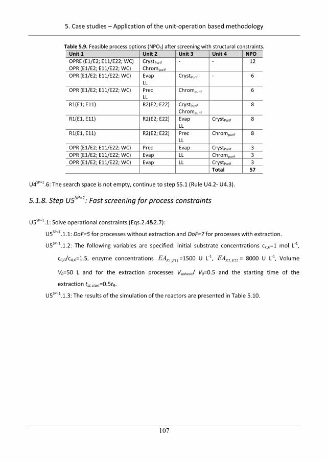
5. Case studies – Application of the unit-operation based methodology
107
Table 5.9. Feasible process options (NPOS) after screening with structural constraints. Unit 1 Unit 2 Unit 3 Unit 4 NPO OPRE (E1/E2; E11/E22; WC) OPR (E1/E2; E11/E22; WC)
CrystPurif
Chrompurif - - 12
OPR (E1/E2; E11/E22; WC) Evap LL
CrystPurif
- 6
OPR (E1/E2; E11/E22; WC) Prec LL
Chrompurif 6
R1(E1; E11) R2(E2; E22) CrystPurif
Chrompurif 8
R1(E1, E11) R2(E2; E22) Evap LL
CrystPurif
8
R1(E1, E11) R2(E2; E22) Prec LL
Chrompurif 8
OPR (E1/E2; E11/E22; WC) Prec Evap CrystPurif 3 OPR (E1/E2; E11/E22; WC) Evap LL Chrompurif 3 OPR (E1/E2; E11/E22; WC) Evap LL CrystPurif 3 Total 57
U4SP=1.6: The search space is not empty, continue to step S5.1 (Rule U4.2- U4.3).
5.1.8. Step U5SP=1: Fast screening for process constraints
U5SP=1.1: Solve operational constraints (Eqs.2.4&2.7):
U5SP=1.1.1: DoF=5 for processes without extraction and DoF=7 for processes with extraction.
U5SP=1.1.2: The following variables are specified: initial substrate concentrations cC,0=1 mol L-1,
cC,0/cA,0=1.5, enzyme concentrations 1, 11E EEA =1500 U L-1, 2, 22E EEA = 8000 U L-1, Volume
V0=50 L and for the extraction processes Vsolvent/ V0=0.5 and the starting time of the
extraction tLL start=0.5tR.
U5SP=1.1.3: The results of the simulation of the reactors are presented in Table 5.10.
137
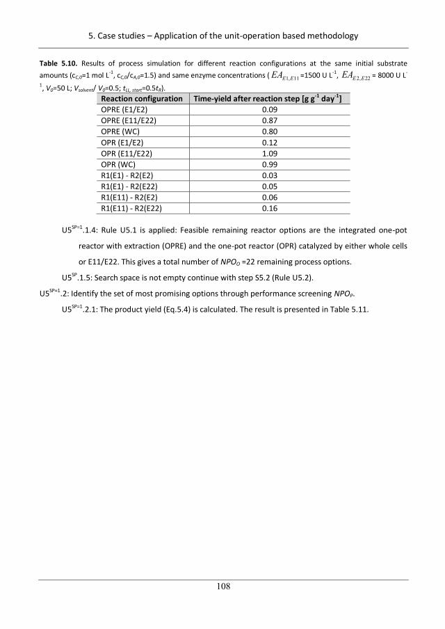
5. Case studies – Application of the unit-operation based methodology
108
Table 5.10. Results of process simulation for different reaction configurations at the same initial substrate amounts (cC,0=1 mol L-1, cC,0/cA,0=1.5) and same enzyme concentrations ( 1, 11E EEA =1500 U L-1, 2, 22E EEA = 8000 U L-
1, V0=50 L; Vsolvent/ V0=0.5; tLL, start=0.5tR). Reaction configuration Time-yield after reaction step [g g-1 day-1] OPRE (E1/E2) 0.09 OPRE (E11/E22) 0.87 OPRE (WC) 0.80 OPR (E1/E2) 0.12 OPR (E11/E22) 1.09 OPR (WC) 0.99 R1(E1) - R2(E2) 0.03 R1(E1) - R2(E22) 0.05 R1(E11) - R2(E2) 0.06 R1(E11) - R2(E22) 0.16
U5SP=1.1.4: Rule U5.1 is applied: Feasible remaining reactor options are the integrated one-pot
reactor with extraction (OPRE) and the one-pot reactor (OPR) catalyzed by either whole cells
or E11/E22. This gives a total number of NPOO =22 remaining process options.
U5SP.1.5: Search space is not empty continue with step S5.2 (Rule U5.2).
U5SP=1.2: Identify the set of most promising options through performance screening NPOP.
U5SP=1.2.1: The product yield (Eq.5.4) is calculated. The result is presented in Table 5.11.
138
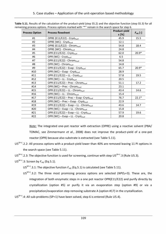
5. Case studies – Application of the unit-operation based methodology
109
Table 5.11. Results of the calculation of the product-yield (step S5.2) and the objective function (step S5.3) for all remaining process options. Process options marked with “*” remain in the search space for step 6.
Process Option Process flowsheet Product yield [%] Fobj [-]
#1 OPRE (E11/E22) - CrystPurif 45.9 15.5 #2 OPRE (WC) - CrystPurif 12.1 #3 OPRE (E11/E22) - ChromPurif 54.8 18.4 #4 OPRE (WC) - ChromPurif 24.8 #5 OPR (E11/E22) - CrystPurif 62.0 20.9* #6 OPR (WC) - CrystPurif 6.5 #7 OPR (E11/E22) - ChromPurif 54.8 #8 OPR (WC) - ChromPurif 14.8 #9 OPR (E11/E22) – Evap - CrystPurif 65.7 20.9*
#10 OPR (WC) – Evap - CrystPurif 28.9 #11 OPR (E11/E22) – LL - CrystPurif 57.8 19.5 #12 OPR (WC) – LL - CrystPurif 20.5 #13 OPR (E11/E22) – Prec - ChromPurif 51.1 17.2 #14 OPR (WC) – Prec - ChromPurif 23.1 #15 OPR (E11/E22) – LL - ChromPurif 43.4 14.6 #16 OPR (WC) – LL - ChromPurif 15.4 #17 OPR (E11/E22) – Prec – Evap -CrystPurif 76.7 22.1* #18 OPR (WC) – Prec – Evap - CrystPurif 22.9 #19 OPR (E11/E22) – Evap – LL - ChromPurif 43.6 14.7 #20 OPR (WC) – Evap – LL - ChromPurif 15.8 #21 OPR (E11/E22) – Evap – LL - CrystPurif 57.9 19.6 #22 OPR (WC) – Evap – LL - CrystPurif 20.8
Note: The integrated one-pot reactor with extraction (OPRE) using a reactive solvent (PBA/
TOMAC, see Zimmermann et al., 2008) does not improve the product-yield of a one-pot
reactor (OPR) because also substrate is extracted (see Table 5.11).
U5SP=1.2.2: All process options with a product-yield lower than 40% are removed leaving 11 PI options in
the search space (see Table 5.11).
U5SP=1.2.3: The objective function is used for screening, continue with step U5SP=1.3 (Rule U5.3).
U5SP=1.3: Screen by Fobj (Eq.5.1).
U5SP=1.3.1: The objective function Fobj (Eq.5.1) is calculated (see Table 5.11).
U5SP=1.3.2: The three most promising process options are selected (NPOP=3). These are, the
integration of both enzymatic steps in a one pot reactor OPR(E11/E22) and purify directly by
crystallization (option #5) or purify it via an evaporation step (option #9) or via a
precipitation/evaporation step removing substrate A (option #17) in the crystallization.
U5SP=1.4: All sub-problems (SP=1) have been solved, step 6 is entered (Rule U5.4).
139
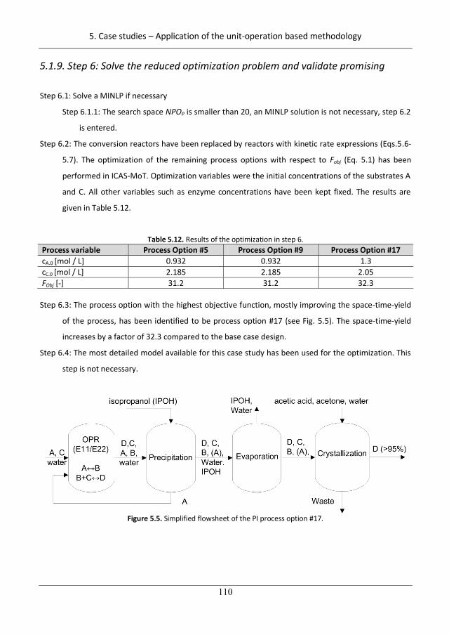
5. Case studies – Application of the unit-operation based methodology
110
5.1.9. Step 6: Solve the reduced optimization problem and validate promising
Step 6.1: Solve a MINLP if necessary
Step 6.1.1: The search space NPOP is smaller than 20, an MINLP solution is not necessary, step 6.2
is entered.
Step 6.2: The conversion reactors have been replaced by reactors with kinetic rate expressions (Eqs.5.6-
5.7). The optimization of the remaining process options with respect to Fobj (Eq. 5.1) has been
performed in ICAS-MoT. Optimization variables were the initial concentrations of the substrates A
and C. All other variables such as enzyme concentrations have been kept fixed. The results are
given in Table 5.12.
Table 5.12. Results of the optimization in step 6. Process variable Process Option #5 Process Option #9 Process Option #17 cA.0 [mol / L] 0.932 0.932 1.3 cC.0 [mol / L] 2.185 2.185 2.05 FObj [-] 31.2 31.2 32.3
Step 6.3: The process option with the highest objective function, mostly improving the space-time-yield
of the process, has been identified to be process option #17 (see Fig. 5.5). The space-time-yield
increases by a factor of 32.3 compared to the base case design.
Step 6.4: The most detailed model available for this case study has been used for the optimization. This
step is not necessary.
Figure 5.5. Simplified flowsheet of the PI process option #17.
140
5. Case studies – Application of the unit-operation based methodology
111
5.1.10. Discussion of the results
The application of the PI synthesis methodology has managed to improve the base-case design. In total
3.5•1011 PI process options have been generated from which through a stepwise reduction of the search
space the best process option has been determined, all on a quantitative basis. Through PI, the base
case design (Mahmoudian et al., 1997) has been improved in the objective function by a factor of 32.3
by process option #17. The reasons are the use of better enzymes (E11 and E22) as well as the
integration of both reaction tasks into one equipment, a one-pot-reactor. The advantage of the latter is
that it drives the reaction beyond the unfavorable equilibrium from A to B by in-situ removal of B by the
second biocatalytic reaction. In addition, the process is simplified since the number of equipment has
decreased from 7 to 4. An analysis of the determined process values of the initial substrate
concentrations in option #5 and option #9 shows that they are on the boundary for the operational
constraint of the crystallization for both substrates (see appendix A6, Eqs.A.6.25-A.6.26) while process
option #17 is bounded due to the solubility of compound A in water (step A2.4.2).
Other studies have shown that fed-batch reactors have the potential to further improve the yield (Hu et
al., 2010; Maru et al., 2002). This option has not been considered in this work.
5.2. Production of hydrogen peroxide
The objective of this case study to find PI-options for the production of hydrogen peroxide, using the
anthraquinone process route as the base-case design (Eul, Moeller & Steiner, 2001). Section 5.2.1
provides introduction to the process; section 5.2.2 describes the base-case design while sections 5.2.3-
5.2.11 describe the step-by-step details of the application of the methodology (unit-operation based).
5.2.1 Introduction
Hydrogen peroxide (H2O2) is a bulk chemical with a market volume of around 3.000.000 metric tons per
year (Zhou, Hammack & Sethi, 2008). Its main applications are in chemical synthesis as well as bleaching
(Goor, Glenneberg & Jacobi, 2007). Reported plant capacities are up to 136.000 metric tons per year
(Eul, Moeller & Steiner, 2001). Hydrogen peroxide is mainly produced by auto-oxidation via
anthraquinones which is the major route used in industry as well as electrochemical synthesis and by
oxidation of alcohols such as isopropanol and methylbenzolalcohol (Eul, Moeller & Steiner, 2001; Goor,
Glenneberg & Jacobi, 2007). Recently, the production of hydrogen peroxide directly from the elements
141
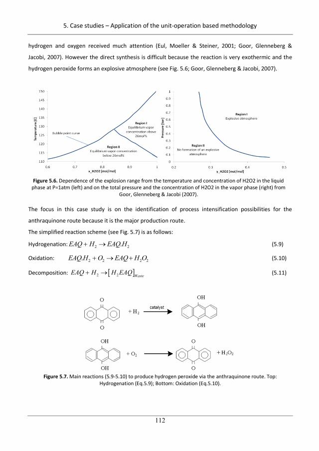
5. Case studies – Application of the unit-operation based methodology
112
hydrogen and oxygen received much attention (Eul, Moeller & Steiner, 2001; Goor, Glenneberg &
Jacobi, 2007). However the direct synthesis is difficult because the reaction is very exothermic and the
hydrogen peroxide forms an explosive atmosphere (see Fig. 5.6; Goor, Glenneberg & Jacobi, 2007).
Figure 5.6. Dependence of the explosion range from the temperature and concentration of H2O2 in the liquid
phase at P=1atm (left) and on the total pressure and the concentration of H2O2 in the vapor phase (right) from Goor, Glenneberg & Jacobi (2007).
The focus in this case study is on the identification of process intensification possibilities for the
anthraquinone route because it is the major production route.
The simplified reaction scheme (see Fig. 5.7) is as follows:
Hydrogenation: 2 2.EAQ H EAQ H (5.9)
Oxidation: 2 2 2 2.EAQ H O EAQ H O (5.10)
Decomposition: 2 2 WasteEAQ H H EAQ (5.11)
Figure 5.7. Main reactions (5.9-5.10) to produce hydrogen peroxide via the anthraquinone route. Top:
Hydrogenation (Eq.5.9); Bottom: Oxidation (Eq.5.10).
142
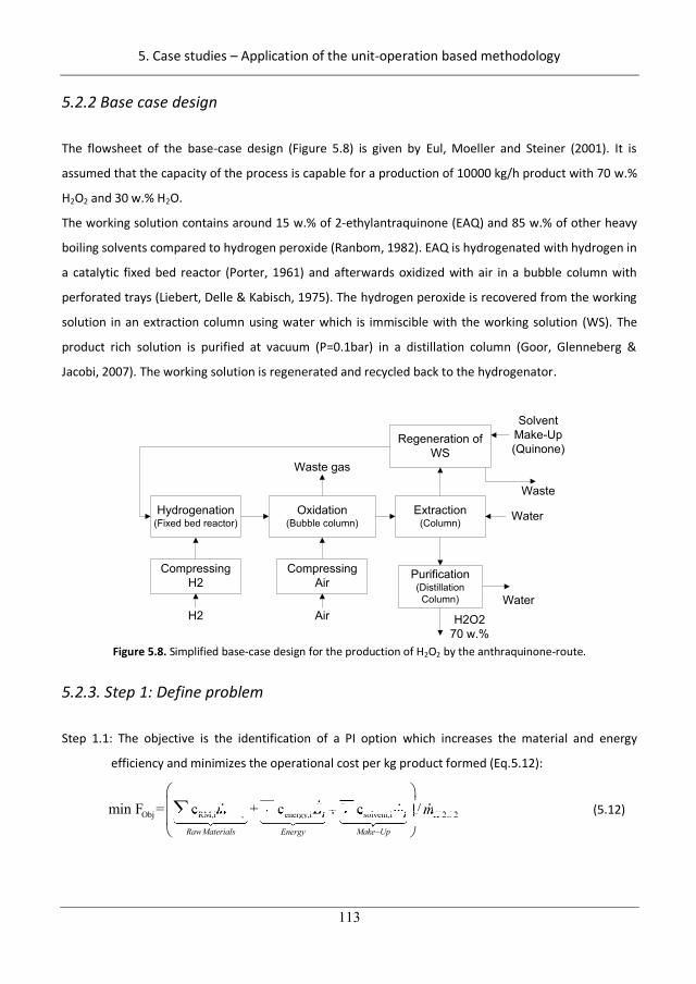
5. Case studies – Application of the unit-operation based methodology
113
5.2.2 Base case design
The flowsheet of the base-case design (Figure 5.8) is given by Eul, Moeller and Steiner (2001). It is
assumed that the capacity of the process is capable for a production of 10000 kg/h product with 70 w.%
H2O2 and 30 w.% H2O.
The working solution contains around 15 w.% of 2-ethylantraquinone (EAQ) and 85 w.% of other heavy
boiling solvents compared to hydrogen peroxide (Ranbom, 1982). EAQ is hydrogenated with hydrogen in
a catalytic fixed bed reactor (Porter, 1961) and afterwards oxidized with air in a bubble column with
perforated trays (Liebert, Delle & Kabisch, 1975). The hydrogen peroxide is recovered from the working
solution in an extraction column using water which is immiscible with the working solution (WS). The
product rich solution is purified at vacuum (P=0.1bar) in a distillation column (Goor, Glenneberg &
Jacobi, 2007). The working solution is regenerated and recycled back to the hydrogenator.
Hydrogenation(Fixed bed reactor)
Extraction(Column)
Regeneration ofWS
Purification(DistillationColumn)
Oxidation(Bubble column)
H2O270 w.%
WaterH2
CompressingH2
SolventMake-Up(Quinone)
Water
Air
CompressingAir
Waste
Waste gas
Figure 5.8. Simplified base-case design for the production of H2O2 by the anthraquinone-route.
5.2.3. Step 1: Define problem
Step 1.1: The objective is the identification of a PI option which increases the material and energy
efficiency and minimizes the operational cost per kg product formed (Eq.5.12):
Obj RM,i , energy,i solvent,i 2 2min F = c + c c /RM i i i H O
RawMaterials Make UpEnergy
m E m m 2 2/ 2m/ii+ c+ c+ c+ c iii+ c cc llc e ,solvent,iRM,i ,RM,i ,RM i ,, solvent isolvent isolvent igy i lgygy,e e gy,energy,ienergy,ienergy ienergy ienergy ienergy ienergy i (5.12)
143
5. Case studies – Application of the unit-operation based methodology
114
Step 1.2: The design scenario is to improve the whole process keeping the anthraquinone production
route. The process scenario is continuous.
Step 1.3: The following operational constraints are set:
The capacity is 10.000 kg/h of H2O2.
The product purity is 70 w.% of H2O2 and 30 w.% & H2O.
The anthraquinone process is fixed.
Due to safety reasons, the concentration of oxygen and hydrogen-peroxide in the hydrogenator
should be zero.
Raw materials: Pure hydrogen and air.
Side-Reactions occur.
Recovery of H2O2 in the last separation step = 0.99.
Working solution (WS) and solvents are fixed.
The operating pressure in the recycle system is fixed to 3.5 bar
Step 1.4: Define performance metric PM.
The following performance metric PM is selected: Safety, efficiency, energy, simplification, waste.
Step 1.5: The maturity is selected to be “medium” using only existing PI technology.
Step 1.6: Translate and PM into logical, structural, operational constraints and performance criteria :
Step 1.6.1: All rules have been applied to gather a set of logical constraints (Eq.2.2). The detailed
results are listed in Table 5.13.
Step 1.6.2: Four PI metrics have been translated to six structural constraints. The result is given in
Table 5.13.
Step 1.6.3: The result of the translation into operational constraints and the PI screening criterion
is given in Table 5.13.
Step 1.7: A base case design exists, step A2 is entered (Rule 1.9).
144
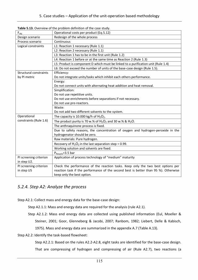
5. Case studies – Application of the unit-operation based methodology
115
Table 5.13. Overview of the problem definition of the case study. Fobj Operational costs per product (Eq.5.12) Design scenario Redesign of the whole process Process scenario Continuous Logical constraints L1: Reaction 1 necessary (Rule 1.1)
L2: Reaction 2 necessary (Rule 1.1) L3: Reaction 1 has to be in the first unit (Rule 1.2) L4: Reaction 1 before or at the same time as Reaction 2 (Rule 1.3) L5: Product is component D which must be linked to a purification unit (Rule 1.4) L6: Do not exceed the number of units of the base-case design (Rule 1.5).
Structural constraints by PI metric
Efficiency: Do not integrate units/tasks which inhibit each others performance. Energy: Do not connect units with alternating heat addition and heat removal. Simplification: Do not use repetitive units. Do not use enrichments before separations if not necessary. Do not use pre-reactors. Waste: Do not add two different solvents to the system.
Operational constraints (Rule 1.6)
The capacity is 10.000 kg/h of H2O2. The product purity is 70 w.% of H2O2 and 30 w.% & H2O. The anthraquinone process is fixed. Due to safety reasons, the concentration of oxygen and hydrogen-peroxide in the hydrogenator should be zero. Raw materials: Pure hydrogen. Recovery of H2O2 in the last separation step = 0.99. Working solution and solvents are fixed. PRecycle=3.5 bar
PI screening criterion in step U2.
Application of process technology of “medium” maturity
PI screening criterion in step U5
Check the performance of the reaction tasks. Keep only the two best options per reaction task if the performance of the second best is better than 95 %). Otherwise keep only the best option.
5.2.4. Step A2: Analyze the process
Step A2.1: Collect mass and energy data for the base-case design:
Step A2.1.1: Mass and energy data are required for the analysis (rule A2.1).
Step A2.1.2: Mass end energy data are collected using published information (Eul, Moeller &
Steiner, 2001; Goor, Glenneberg & Jacobi, 2007; Ranbom, 1982; Liebert, Delle & Kabisch,
1975). Mass and energy data are summarized in the appendix A.7 (Table A.13).
Step A2.2: Identify the task-based flowsheet:
Step A2.2.1: Based on the rules A2.2-A2.8, eight tasks are identified for the base-case design.
That are compressing of hydrogen and compressing of air (Rule A2.7), two reactions (a
145
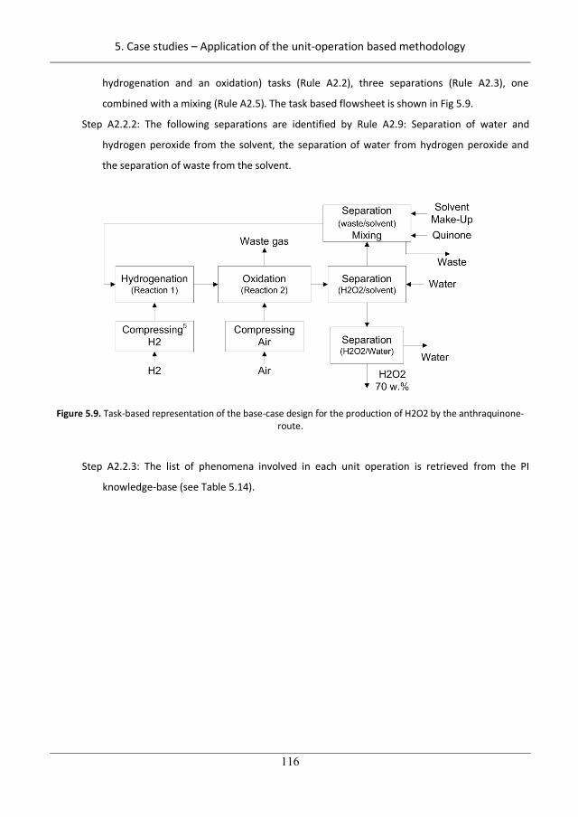
5. Case studies – Application of the unit-operation based methodology
116
hydrogenation and an oxidation) tasks (Rule A2.2), three separations (Rule A2.3), one
combined with a mixing (Rule A2.5). The task based flowsheet is shown in Fig 5.9.
Step A2.2.2: The following separations are identified by Rule A2.9: Separation of water and
hydrogen peroxide from the solvent, the separation of water from hydrogen peroxide and
the separation of waste from the solvent.
Figure 5.9. Task-based representation of the base-case design for the production of H2O2 by the anthraquinone-route.
Step A2.2.3: The list of phenomena involved in each unit operation is retrieved from the PI
knowledge-base (see Table 5.14).
146
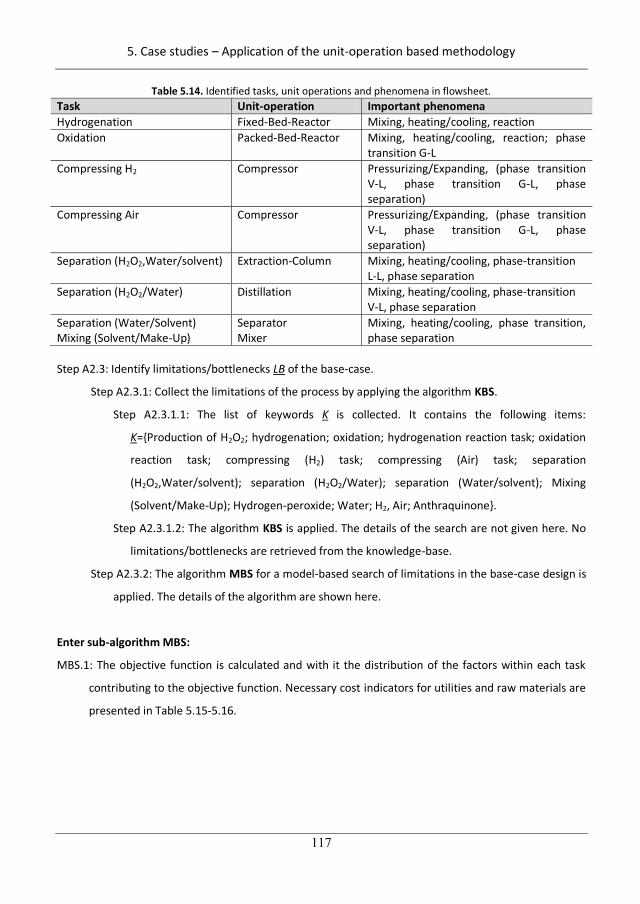
5. Case studies – Application of the unit-operation based methodology
117
Table 5.14. Identified tasks, unit operations and phenomena in flowsheet. Task Unit-operation Important phenomena Hydrogenation Fixed-Bed-Reactor Mixing, heating/cooling, reaction Oxidation Packed-Bed-Reactor Mixing, heating/cooling, reaction; phase
transition G-L Compressing H2 Compressor Pressurizing/Expanding, (phase transition
V-L, phase transition G-L, phase separation)
Compressing Air Compressor Pressurizing/Expanding, (phase transition V-L, phase transition G-L, phase separation)
Separation (H2O2,Water/solvent) Extraction-Column Mixing, heating/cooling, phase-transition L-L, phase separation
Separation (H2O2/Water) Distillation Mixing, heating/cooling, phase-transition V-L, phase separation
Separation (Water/Solvent) Mixing (Solvent/Make-Up)
Separator Mixer
Mixing, heating/cooling, phase transition, phase separation
Step A2.3: Identify limitations/bottlenecks LB of the base-case.
Step A2.3.1: Collect the limitations of the process by applying the algorithm KBS.
Step A2.3.1.1: The list of keywords K is collected. It contains the following items:
K={Production of H2O2; hydrogenation; oxidation; hydrogenation reaction task; oxidation
reaction task; compressing (H2) task; compressing (Air) task; separation
(H2O2,Water/solvent); separation (H2O2/Water); separation (Water/solvent); Mixing
(Solvent/Make-Up); Hydrogen-peroxide; Water; H2, Air; Anthraquinone}.
Step A2.3.1.2: The algorithm KBS is applied. The details of the search are not given here. No
limitations/bottlenecks are retrieved from the knowledge-base.
Step A2.3.2: The algorithm MBS for a model-based search of limitations in the base-case design is
applied. The details of the algorithm are shown here.
Enter sub-algorithm MBS:
MBS.1: The objective function is calculated and with it the distribution of the factors within each task
contributing to the objective function. Necessary cost indicators for utilities and raw materials are
presented in Table 5.15-5.16.
147
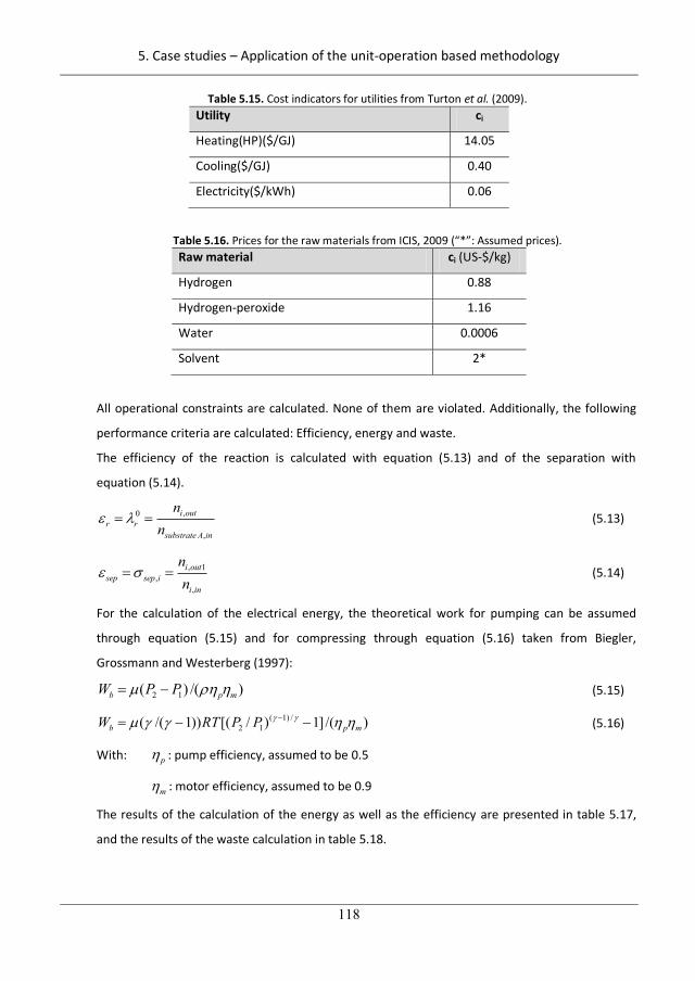
5. Case studies – Application of the unit-operation based methodology
118
Table 5.15. Cost indicators for utilities from Turton et al. (2009). Utility ci
Heating(HP)($/GJ) 14.05
Cooling($/GJ) 0.40
Electricity($/kWh) 0.06
Table 5.16. Prices for the raw materials from ICIS, 2009 (“*”: Assumed prices). Raw material ci (US-$/kg)
Hydrogen 0.88
Hydrogen-peroxide 1.16
Water 0.0006
Solvent 2*
All operational constraints are calculated. None of them are violated. Additionally, the following
performance criteria are calculated: Efficiency, energy and waste.
The efficiency of the reaction is calculated with equation (5.13) and of the separation with
equation (5.14).
,0
,
i outr r
substrate A in
nn
(5.13)
, 1,
,
i outsep sep i
i in
nn
(5.14)
For the calculation of the electrical energy, the theoretical work for pumping can be assumed
through equation (5.15) and for compressing through equation (5.16) taken from Biegler,
Grossmann and Westerberg (1997):
2 1( ) /( )b p mW P P (5.15)
( 1) /2 1( /( 1)) [( / ) 1]/( )b p mW RT P P (5.16)
With: p : pump efficiency, assumed to be 0.5
m : motor efficiency, assumed to be 0.9
The results of the calculation of the energy as well as the efficiency are presented in table 5.17,
and the results of the waste calculation in table 5.18.
148

5. Case studies – Application of the unit-operation based methodology
119
Table 5.17. Calculated efficiencies and energy consumption. Task Unit-operation Efficiencies Energy (GJ/h) Hydrogenation Fixed-Bed-
Reactor 0.99 for hydrogen 22.6
Oxidation Packed-Bed-Reactor
0.99 for hydrogen-peroxide 0.65 for oxygen
18.5
Compressing H2 Compressor - 4.1 Compressing Air Compressor - 9.6 Separation (H2O2,Water/solvent)
Extraction-Column
0.99 1.7
Separation (H2O2/Water) Distillation 0.99 44.5
Separation (Water/Solvent) Mixing (Solvent/Make-Up)
Separator Mixer
- -
Table 5.18. Waste generation in each task.
Task Waste [kg/h] What
Oxidation 41000 Purge (N2)
Separation (Water/Solvent) Mixing (Solvent/Make-Up)
3000 Purge (mostly water,
QC9H12, N2, H2O2)
Separation (H2O2/Water) 11000 99.9% water
MBS.2: Based on their contribution to the Fobj (Fig 5.10) and on the energy (Fig 5.11), waste (Table 5.18)
and efficiency (Table 5.17), the following limitations/bottlenecks are added LB={LB1: Low
efficiency in the oxidation; LB2: Large amount of waste in oxidation; LB3: Large amount of waste in
separation (H2O2/Water); LB4: High energy/High costs for compressing air; LB5: High energy/High
costs for separation H2O2/water; LB6: High energy for hydrogenation; LB7: High energy for
oxidation; LB8: High costs for hydrogen; LB9: High costs for make-up solvent; LB10: High costs for
waste stream}.
149

5. Case studies – Application of the unit-operation based methodology
120
Compressor H2
Compressor Air
RM: Water
Energy Hydrogenation
Energy Oxidation
Energy Extraction
Energy Purification
RM: Hydrogen
Make-Up solvent
Loss of H2O2 with Gas
Loss of H2O2 with WS
Figure 5.10. Contribution to the objective function.
Compressor H2
Compressor Air
Hydrogenation
Oxidation
Extraction
Purification
Figure 5.11. Contribution to the energy consumption.
MBS.3: No operational constraint is violated.
MBS.4: Because the operating costs are selected as objective function Fobj, “SustainPro” is used to
calculate the task responsible for the most negative impact on two important mass and energy
indicators (MVA and EWC). Based on the analysis of the indicators (Table 5.19-5.20), the following
additional limitations/bottlenecks are: LB11: Large amount of water necessary for extraction.
150
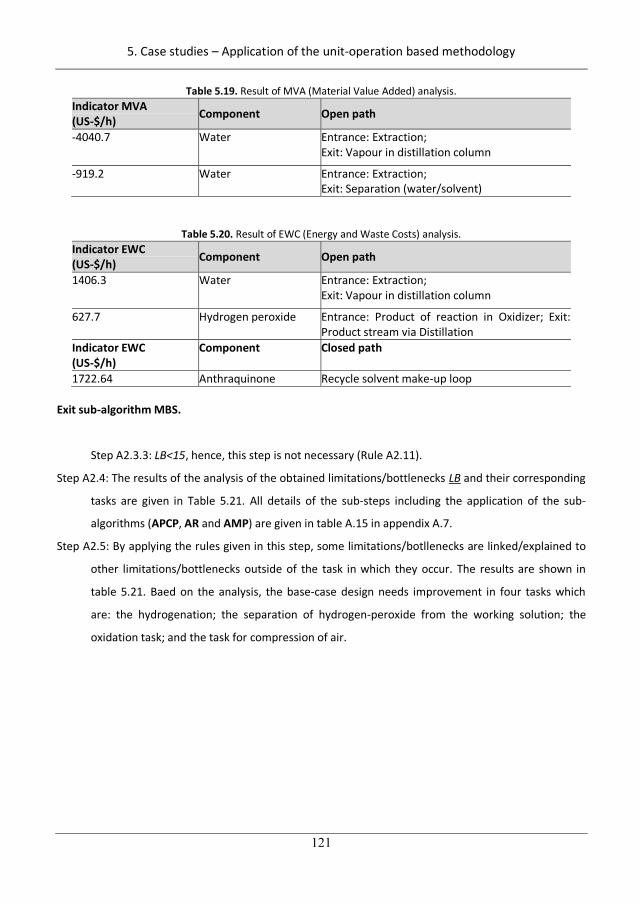
5. Case studies – Application of the unit-operation based methodology
121
Table 5.19. Result of MVA (Material Value Added) analysis. Indicator MVA (US-$/h) Component Open path
-4040.7 Water Entrance: Extraction; Exit: Vapour in distillation column
-919.2 Water Entrance: Extraction; Exit: Separation (water/solvent)
Table 5.20. Result of EWC (Energy and Waste Costs) analysis. Indicator EWC (US-$/h) Component Open path
1406.3 Water Entrance: Extraction; Exit: Vapour in distillation column
627.7 Hydrogen peroxide Entrance: Product of reaction in Oxidizer; Exit: Product stream via Distillation
Indicator EWC (US-$/h)
Component Closed path
1722.64 Anthraquinone Recycle solvent make-up loop
Exit sub-algorithm MBS.
Step A2.3.3: LB<15, hence, this step is not necessary (Rule A2.11).
Step A2.4: The results of the analysis of the obtained limitations/bottlenecks LB and their corresponding
tasks are given in Table 5.21. All details of the sub-steps including the application of the sub-
algorithms (APCP, AR and AMP) are given in table A.15 in appendix A.7.
Step A2.5: By applying the rules given in this step, some limitations/botllenecks are linked/explained to
other limitations/bottlenecks outside of the task in which they occur. The results are shown in
table 5.21. Baed on the analysis, the base-case design needs improvement in four tasks which
are: the hydrogenation; the separation of hydrogen-peroxide from the working solution; the
oxidation task; and the task for compression of air.
151
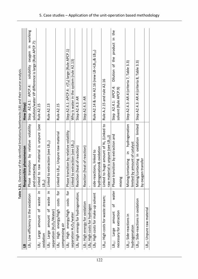
5. Case studies – Application of the unit-operation based methodology
122
Tabl
e 5.
21. O
verv
iew
of t
he id
entif
ied
limita
tions
/bot
tlene
cks (
LB) a
nd th
eir s
ourc
e an
alys
is.
LB
Resp
onsib
le p
heno
men
on
How
(Ste
p)
LB1:
Low
effi
cien
cy in
the
oxid
atio
n Ph
ase
tran
sitio
n by
rel
ativ
e vo
latil
ity
and
cont
actin
g St
ep
A2.4
.1:
APCP
.4:
so
lubi
lity
oxyg
en
in
wor
king
so
lutio
n/w
ater
VP
diffe
renc
e is
larg
e (R
ule
APCP
.7):
LB
2: La
rge
amou
nt
of
was
te
in
oxid
atio
n Li
nked
to
raw
mat
eria
l is
unpu
re (
see
LB14
) Ru
le A
2.15
LB3:
Larg
e am
ount
of
w
aste
in
se
para
tion
(H2O
2/W
ater
) Li
nked
to e
xtra
ctio
n (s
ee LB
11)
Rule
A2.
13
LB4:
High
en
ergy
/Hig
h co
sts
for
com
pres
sing
air
Link
ed to
LB14
: Unp
ure
raw
mat
eria
l Ru
le A
2.15
LB5:
High
en
ergy
/Hig
h co
sts
for
sepa
ratio
n H
2O2/
wat
er
Phas
e tr
ansit
ion
by re
lativ
e vo
latil
ity
Step
A2.
4.1:
APC
P.4:
r(T
B) la
rge
(Rul
e AP
CP.1
) Li
nked
to e
xtra
ctio
n (s
ee LB
11)
Why
is w
ater
in th
e sy
stem
(rul
e A2
.13)
LB
6: Hi
gh e
nerg
y fo
r hyd
roge
natio
n;
Reac
tion
(hea
t of r
eact
ion)
St
ep A
2.4.
3: A
R
LB7:
High
ene
rgy
for o
xida
tion
Reac
tion
(hea
t of r
eact
ion)
St
ep A
2.4.
3: A
R LB
8: Hi
gh co
sts f
or h
ydro
gen
-
LB9:
High
cost
s for
mak
e-up
solv
ent
side-
reac
tions
, lin
ked
to
hydr
ogen
atio
n& o
xida
tion
Rule
A2.
14 &
rule
A2.
16 (n
ew LB
->LB
12&
LB13
)
LB10
: Hig
h co
sts f
or w
aste
stre
am;
Link
ed to
hug
e am
ount
of N
2 (Li
nked
to
raw
mat
eria
l is u
npur
e (s
ee L
B 14))
Ru
le A
.2.1
5 an
d ru
le A
2.16
LB11
: La
rge
amou
nt
of
wat
er
nece
ssar
y fo
r ext
ract
ion
Phas
e tr
ansit
ion
by e
xtra
ctio
n an
d
mix
ing
Step
A2.
4.1:
APC
P.4:
Di
lutio
n of
the
pro
duct
in
the
solv
ent (
Rule
APC
P.9)
LB12
: Sid
e-re
actio
ns in
hy
drog
enat
ion
Mix
ing/
cont
actin
g in
hy
drog
enat
ion
limite
d by
am
ount
of c
atal
yst
Step
A2.
4.3:
AR.
4 (c
riter
ia 7
, Tab
le 3
.3)
LB13
: Sid
e-re
actio
ns in
oxi
datio
n M
ixin
g/co
ntac
ting
in o
xida
tion
limite
d by
oxy
gen
tran
sfer
St
ep A
2.4.
3: A
R.4
(crit
eria
8, T
able
3.3
)
LB14
: Unp
ure
raw
mat
eria
l
152
5. Case studies – Application of the unit-operation based methodology
123
Step A2.6: The maturity is selected to be ”medium” (step 1). Hence, step U2 is entered.
5.2.5. Step U2: Collect PI equipment
Step U2.1: Collect potential PI equipment:
Step U2.1.1: The list of keywords KPI for PI equipment search includes all identified
limitations/bottlenecks and the corresponding phenomena (see Table 5.21).
Step U2.1.2: The algorithm KBS is applied to retrieve potential equipment in a list . The results
are shown in the table A.16 in appendix A.7.
Step U2.2: Pre-screen candidate PI equipment for feasibility:
Step U2.2.1-U2.2.3: The sub-steps are performed. The result of the screening is shown in
table 5.22.
Step U2.2.4: Pre-screen candidate PI equipment for maturity: The sub-steps are performed. The
result of the screening is presented in table 5.22.
Note: For example, the integration of oxidation and purification in a reactive distillation is
screened out due to the operating window analysis (OPW). The reason for removing this
option from the search space is that the oxidation reaction has to take place at pressure
above the atmospheric pressure in order to achieve the transport of oxygen into the liquid
while due to the safety reasons the purification of hydrogen peroxide must take place at low
pressures (see Fig. 5.6). Another example for the screening is a unit operation considering a
solid product such as a reactive crystallizer which is removed due to not matching phases
(see Table 5.22).
153
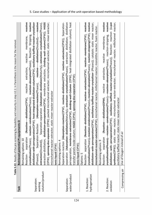
5. Case studies – Application of the unit-operation based methodology
124
Tabl
e 5.
22. R
esul
ts o
f the
pre
-scr
eeni
ng b
y fe
asib
ility
and
mat
urity
in st
ep U
2.2.
In P
aren
thes
is is
the
reas
on fo
r the
rem
oval
. Ta
sk
Retr
ieve
d po
tent
ial P
I equ
ipm
ents
Sepa
ratio
n:
wor
king
so
lutio
n/pr
oduc
t
Rem
aini
ng o
ptio
ns: 1
0 Re
actio
n -
sepa
ratio
n (R
eact
ive
dist
illat
ion(
OPW
), re
activ
e ex
trac
tion,
re
activ
e m
embr
ane,
re
activ
e cr
ysta
lliza
tion(
Phas
es),
reac
tion
cond
ensa
tion(
Phas
es),
reac
tion-
abso
rptio
n(Ph
ases
), Re
actio
n St
rippi
ng,
reac
tive
dist
illat
ion
with
per
vapo
ratio
n(O
PW);
heat
-inte
grat
ed d
istill
atio
n co
lum
n(O
PW),
oscil
lato
ry b
affle
d re
acto
r-cr
ysta
llize
r (P
hase
s)),
Sepa
ratio
n-Re
actio
n (A
bsor
ptio
n-re
actio
n(Ph
ases
), re
activ
e di
still
atio
n(Do
uble
d),
reac
tive
extr
actio
n(Do
uble
d)),
Se
para
tion-
sepa
ratio
n (A
dsor
ptio
n di
still
atio
n(M
atur
ity),
extr
actio
n cr
ysta
lliza
tion(
Phas
es),
extr
actio
n-di
still
atio
n, d
istill
atio
n-pe
rvap
orat
ion(
OPW
), m
embr
ane
extr
actio
n, d
ivid
ing
wal
l co
lum
n(O
PW));
HIG
EE
(OPW
), sp
inni
ng d
isc se
para
tor (
OPW
); pa
cked
mic
roch
anne
l ext
ract
or; m
icro
chan
nel e
xtra
ctor
; sta
tic m
ixer
ext
ract
or;
mic
roch
anne
l rea
ctor
-ext
ract
or, s
tatic
mix
er re
acto
r-ex
trac
tor
Ioni
c liq
uid
(OPW
)
Sepa
ratio
n:
wat
er/p
rodu
ct
Rem
aini
ng o
ptio
ns: 4
Se
para
tion-
reac
tion
(Abs
orpt
ion-
reac
tion(
OPW
), re
activ
e di
still
atio
n(O
PW),
reac
tive
extr
actio
n(O
PW)),
Sep
arat
ion-
sepa
ratio
n (A
dsor
ptio
n di
still
atio
n(M
atur
ity),
extr
actio
n cr
ysta
lliza
tion(
Phas
es),
extr
actio
n di
still
atio
n; d
istill
atio
n pe
rvap
orat
ion,
mem
bran
e ex
trac
tion(
OPW
), di
vidi
ng w
all C
olum
n (O
PW),
heat
-inte
grat
ed d
istill
atio
n co
lum
n); h
eat
tran
sfer
pan
els i
nsid
e co
lum
n; H
IGEE
(OPW
), sp
inni
ng d
isc se
para
tor (
OPW
);
Ioni
c liq
uid
(OPW
);
1. R
eact
ion:
hy
drog
enat
ion
Opt
ions
: 5
Reac
tion-
sep
arat
ion
(Rea
ctiv
e di
still
atio
n(O
PW),
reac
tive
extr
actio
n(O
PW),
reac
tive
mem
bran
e(O
PW),
reac
tive
crys
talli
zatio
n(Ph
ases
), re
actio
n co
nden
satio
n(Ph
ases
), re
actio
n-ab
sorp
tion(
Phas
es),
reac
tion-
strip
ping
(OPW
), re
activ
e di
still
atio
n w
ith p
erva
pora
tion(
OPW
), os
cilla
tory
baf
fled
reac
tor-
crys
talli
zer
(Pha
ses)
); ca
taly
tic s
tatic
mix
er r
eact
or;
mic
roch
anne
l rea
ctor
-ext
ract
or(O
PW),
mic
roch
anne
l rea
ctor
, mill
icha
nnel
reac
tor;
mon
olith
ic re
acto
r, fo
am re
acto
r.
2. R
eact
ion:
ox
idat
ion
Rem
aini
ng o
ptio
ns: 9
Re
actio
n-
sepa
ratio
n (R
eact
ive
dist
illat
ion(
OPW
), re
activ
e ex
trac
tion,
re
activ
e m
embr
ane,
re
activ
e cr
ysta
lliza
tion(
Phas
es),
reac
tion
cond
ensa
tion(
Phas
es),
reac
tion-
abso
rptio
n(Ph
ases
), re
actio
n-st
rippi
ng,
reac
tive
dist
illat
ion
with
per
vapo
ratio
n(O
PW),
osci
llato
ry b
affle
d re
acto
r-cr
ysta
llize
r(Ph
ases
)), R
eact
ion-
rea
ctio
n (1
-pot
sy
nthe
sis(O
PW));
sta
tic m
ixer
rea
ctor
; m
icro
chan
nel
reac
tor-
extr
acto
r; m
icro
chan
nel
reac
tor;
mill
icha
nnel
rea
ctor
; os
cilla
tory
baf
fled
reac
tor;
stat
ic m
ixer
reac
tor-
extr
acto
r Co
mpr
essin
g ai
r U
se o
f Oxy
gen
inst
ead
of a
ir
154
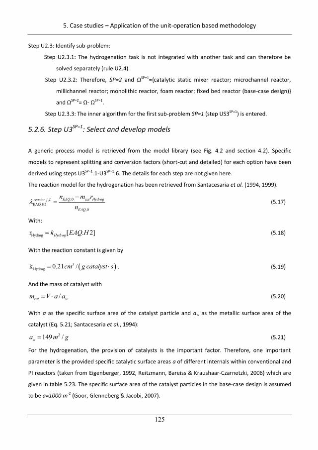
5. Case studies – Application of the unit-operation based methodology
125
Step U2.3: Identify sub-problem:
Step U2.3.1: The hydrogenation task is not integrated with another task and can therefore be
solved separately (rule U2.4).
Step U2.3.2: Therefore, SP=2 and SP=1={catalytic static mixer reactor; microchannel reactor,
millichannel reactor; monolithic reactor, foam reactor; fixed bed reactor (base-case design)}
and SP=2= - SP=1.
Step U2.3.3: The inner algorithm for the first sub-problem SP=1 (step US3SP=1) is entered.
5.2.6. Step U3SP=1: Select and develop models
A generic process model is retrieved from the model library (see Fig. 4.2 and section 4.2). Specific
models to represent splitting and conversion factors (short-cut and detailed) for each option have been
derived using steps U3SP=1.1-U3SP=1.6. The details for each step are not given here.
The reaction model for the hydrogenation has been retrieved from Santacesaria et al. (1994, 1999).
,0,EAQ.H2
,0
EAQ cat Hydrogreactor j L
EAQ
n m rn
(5.17)
With:
Hydrogr [ . 2]Hydrogk EAQ H (5.18)
With the reaction constant is given by
3Hydrogk 0.21 /cm g catalyst s . (5.19)
And the mass of catalyst with
/cat wm V a a (5.20)
With a as the specific surface area of the catalyst particle and aw as the metallic surface area of the
catalyst (Eq. 5.21; Santacesaria et al., 1994): 2149 /wa m g (5.21)
For the hydrogenation, the provision of catalysts is the important factor. Therefore, one important
parameter is the provided specific catalytic surface areas a of different internals within conventional and
PI reactors (taken from Eigenberger, 1992, Reitzmann, Bareiss & Kraushaar-Czarnetzki, 2006) which are
given in table 5.23. The specific surface area of the catalyst particles in the base-case design is assumed
to be a=1000 m-1 (Goor, Glenneberg & Jacobi, 2007).
155
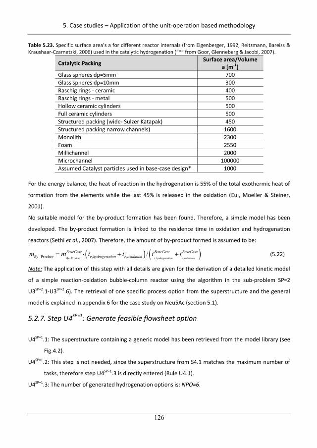
5. Case studies – Application of the unit-operation based methodology
126
Table 5.23. Specific surface area’s a for different reactor internals (from Eigenberger, 1992, Reitzmann, Bareiss & Kraushaar-Czarnetzki, 2006) used in the catalytic hydrogenation (“*” from Goor, Glenneberg & Jacobi, 2007).
Catalytic Packing Surface area/Volume a [m-1]
Glass spheres dp=5mm 700 Glass spheres dp=10mm 300 Raschig rings - ceramic 400 Raschig rings - metal 500 Hollow ceramic cylinders 500 Full ceramic cylinders 500 Structured packing (wide- Sulzer Katapak) 450 Structured packing narrow channels) 1600 Monolith 2300 Foam 2550 Millichannel 2000 Microchannel 100000 Assumed Catalyst particles used in base-case design* 1000
For the energy balance, the heat of reaction in the hydrogenation is 55% of the total exothermic heat of
formation from the elements while the last 45% is released in the oxidation (Eul, Moeller & Steiner,
2001).
No suitable model for the by-product formation has been found. Therefore, a simple model has been
developed. The by-product formation is linked to the residence time in oxidation and hydrogenation
reactors (Sethi et al., 2007). Therefore, the amount of by-product formed is assumed to be:
Pr , ,Pr , , /By oduct r hydrogenation r oxidation
BaseCase BaseCase BaseCaseBy oduct r hydrogenation r oxidationm m t t t t (5.22)
Note: The application of this step with all details are given for the derivation of a detailed kinetic model
of a simple reaction-oxidation bubble-column reactor using the algorithm in the sub-problem SP=2
U3SP=2.1-U3SP=2.6). The retrieval of one specific process option from the superstructure and the general
model is explained in appendix 6 for the case study on Neu5Ac (section 5.1).
5.2.7. Step U4SP=1: Generate feasible flowsheet option
U4SP=1.1: The superstructure containing a generic model has been retrieved from the model library (see
Fig.4.2).
U4SP=1.2: This step is not needed, since the superstructure from S4.1 matches the maximum number of
tasks, therefore step U4SP=1.3 is directly entered (Rule U4.1).
U4SP=1.3: The number of generated hydrogenation options is: NPO=6.
156
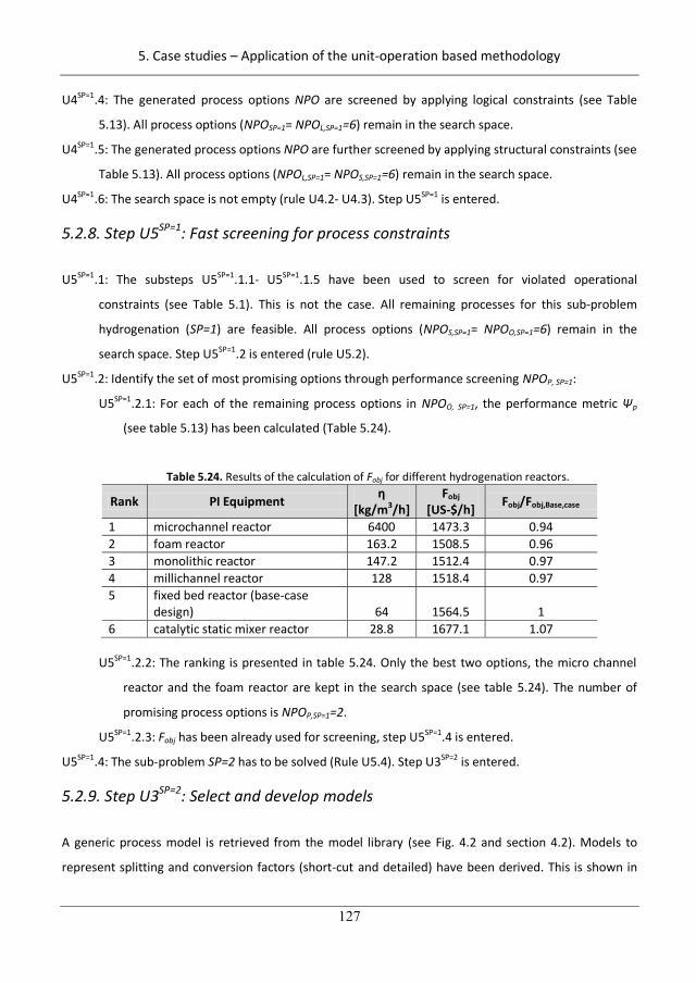
5. Case studies – Application of the unit-operation based methodology
127
U4SP=1.4: The generated process options NPO are screened by applying logical constraints (see Table
5.13). All process options (NPOSP=1= NPOL,SP=1=6) remain in the search space.
U4SP=1.5: The generated process options NPO are further screened by applying structural constraints (see
Table 5.13). All process options (NPOL,SP=1= NPOS,SP=1=6) remain in the search space.
U4SP=1.6: The search space is not empty (rule U4.2- U4.3). Step U5SP=1 is entered.
5.2.8. Step U5SP=1: Fast screening for process constraints
U5SP=1.1: The substeps U5SP=1.1.1- U5SP=1.1.5 have been used to screen for violated operational
constraints (see Table 5.1). This is not the case. All remaining processes for this sub-problem
hydrogenation (SP=1) are feasible. All process options (NPOS,SP=1= NPOO,SP=1=6) remain in the
search space. Step U5SP=1.2 is entered (rule U5.2).
U5SP=1.2: Identify the set of most promising options through performance screening NPOP, SP=1:
U5SP=1.2.1: For each of the remaining process options in NPOO, SP=1, the performance metric p
(see table 5.13) has been calculated (Table 5.24).
Table 5.24. Results of the calculation of Fobj for different hydrogenation reactors.
Rank PI Equipment [kg/m3/h]
Fobj [US-$/h] Fobj/Fobj,Base,case
1 microchannel reactor 6400 1473.3 0.94 2 foam reactor 163.2 1508.5 0.96 3 monolithic reactor 147.2 1512.4 0.97 4 millichannel reactor 128 1518.4 0.97 5 fixed bed reactor (base-case
design) 64 1564.5 1 6 catalytic static mixer reactor 28.8 1677.1 1.07
U5SP=1.2.2: The ranking is presented in table 5.24. Only the best two options, the micro channel
reactor and the foam reactor are kept in the search space (see table 5.24). The number of
promising process options is NPOP,SP=1=2.
U5SP=1.2.3: Fobj has been already used for screening, step U5SP=1.4 is entered.
U5SP=1.4: The sub-problem SP=2 has to be solved (Rule U5.4). Step U3SP=2 is entered.
5.2.9. Step U3SP=2: Select and develop models
A generic process model is retrieved from the model library (see Fig. 4.2 and section 4.2). Models to
represent splitting and conversion factors (short-cut and detailed) have been derived. This is shown in
157
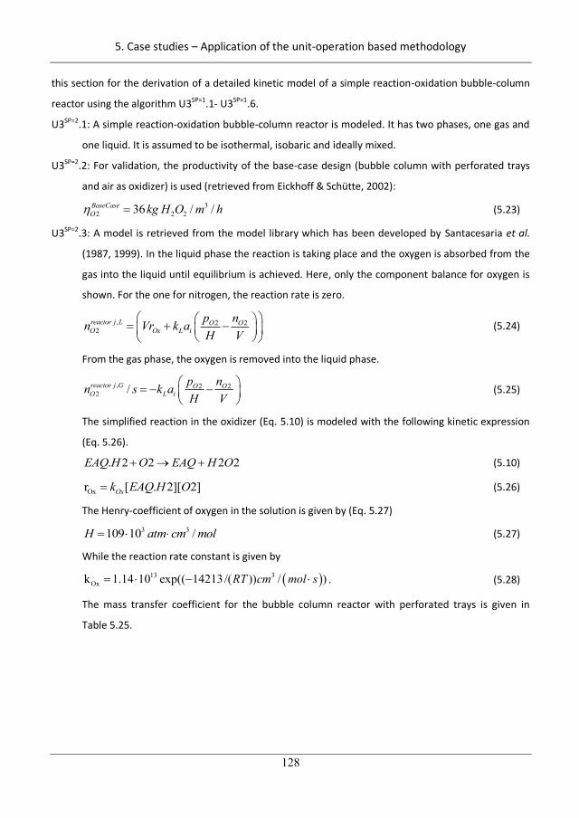
5. Case studies – Application of the unit-operation based methodology
128
this section for the derivation of a detailed kinetic model of a simple reaction-oxidation bubble-column
reactor using the algorithm U3SP=1.1- U3SP=1.6.
U3SP=2.1: A simple reaction-oxidation bubble-column reactor is modeled. It has two phases, one gas and
one liquid. It is assumed to be isothermal, isobaric and ideally mixed.
U3SP=2.2: For validation, the productivity of the base-case design (bubble column with perforated trays
and air as oxidizer) is used (retrieved from Eickhoff & Schütte, 2002):
32 2 236 / /BaseCase
O kg H O m h (5.23)
U3SP=2.3: A model is retrieved from the model library which has been developed by Santacesaria et al.
(1987, 1999). In the liquid phase the reaction is taking place and the oxygen is absorbed from the
gas into the liquid until equilibrium is achieved. Here, only the component balance for oxygen is
shown. For the one for nitrogen, the reaction rate is zero.
, 2 22
reactor j L O OO Ox L i
p nn Vr k aH V
(5.24)
From the gas phase, the oxygen is removed into the liquid phase.
, 2 22 /reactor j G O O
O L ip nn s k aH V
(5.25)
The simplified reaction in the oxidizer (Eq. 5.10) is modeled with the following kinetic expression
(Eq. 5.26).
. 2 2 2 2EAQ H O EAQ H O (5.10)
Oxr [ . 2][ 2]Oxk EAQ H O (5.26)
The Henry-coefficient of oxygen in the solution is given by (Eq. 5.27) 3 3109 10 /H atm cm mol (5.27)
While the reaction rate constant is given by 13 3
Oxk 1.14 10 exp(( 14213/( )) / )RT cm mol s . (5.28)
The mass transfer coefficient for the bubble column reactor with perforated trays is given in
Table 5.25.
158
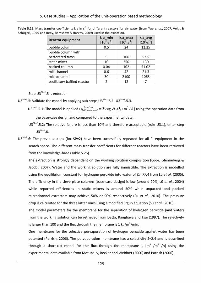
5. Case studies – Application of the unit-operation based methodology
129
Table 5.25. Mass transfer coefficients kLa in s-1 for different reactors for air-water (from Yue et al., 2007, Voigt & Schügerl, 1979 and Reay, Ramshaw & Harvey, 2009) used in the oxidation.
Reactor equipment kLa_min [102·s-1]
kLa_max [102·s-1]
kLa_avg [102·s-1]
bubble column 0.5 24 12.25 bubble column with perforated trays 5 100 52.5 static mixer 10 250 130 packed column 0.04 102 51.02 millichannel 0.6 42 21.3 microchannel 30 2100 1065 oscillatory baffled reactor 2 12 7
Step U3SP=2.5 is entered.
U3SP=2.5: Validate the model by applying sub-steps U3SP=1.5.1- U3SP=1.5.3.
U3SP=2.5.1: The model is applied ( 32, 2 239 / /BaseCase
O calculated kg H O m h ) using the operation data from
the base-case design and compared to the experimental data.
U3SP=2.5.2: The relative failure is less than 10% and therefore acceptable (rule U3.1), enter step
U3SP=2.6.
U3SP=2.6: The previous steps (for SP=2) have been successfully repeated for all PI equipment in the
search space. The different mass transfer coefficients for different reactors have been retrieved
from the knowledge-base (Table 5.25).
The extraction is strongly dependent on the working solution composition (Goor, Glenneberg &
Jacobi, 2007). Water and the working solution are fully immiscible. The extraction is modelled
using the equilibrium constant for hydrogen peroxide into water of KE=77.4 from Lü et al. (2005).
The efficiency in the sieve plate columns (base-case design) is low (around 20%, Lü et al., 2004)
while reported efficiencies in static mixers is around 50% while unpacked and packed
microchannel-extractors may achieve 50% or 90% respectively (Su et al., 2010). The pressure
drop is calculated for the three latter ones using a modified Ergun equation (Su et al., 2010).
The model parameters for the membrane for the separation of hydrogen peroxide (and water)
from the working solution can be retrieved from Datta, Ranghava and Tsai (1997). The selectivity
is larger than 100 and the flux through the membrane is 1 kg/m2/min.
One membrane for the selective pervaporation of hydrogen peroxide against water has been
patented (Parrish, 2006). The pervaporation membrane has a selectivity S=2.4 and is described
through a short-cut model for the flux through the membrane Ji [m3 /m2 /h] using the
experimental data available from Motupally, Becker and Weidner (2000) and Parrish (2006).
159
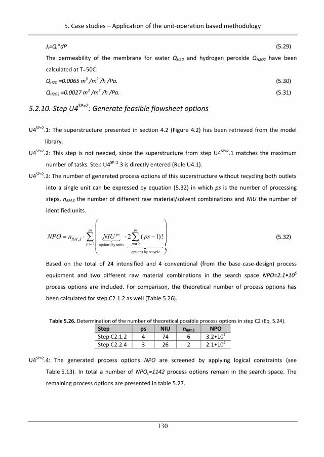
5. Case studies – Application of the unit-operation based methodology
130
Ji=Qi*dP (5.29)
The permeability of the membrane for water QH2O and hydrogen peroxide QH2O2 have been
calculated at T=50C:
QH2O =0.0065 m3 /m2 /h /Pa. (5.30)
QH2O2 =0.0027 m3 /m2 /h /Pa. (5.31)
5.2.10. Step U4SP=2: Generate feasible flowsheet options
U4SP=2.1: The superstructure presented in section 4.2 (Figure 4.2) has been retrieved from the model
library.
U4SP=2.2: This step is not needed, since the superstructure from step U4SP=2.1 matches the maximum
number of tasks. Step U4SP=2.3 is directly entered (Rule U4.1).
U4SP=2.3: The number of generated process options of this superstructure without recycling both outlets
into a single unit can be expressed by equation (5.32) in which ps is the number of processing
steps, nRM,S the number of different raw material/solvent combinations and NIU the number of
identified units.
,2 2options by units
options by recycle
2 ( 1)!ps ps
psRM S
ps psNPO n NIU psNIU 2NIU 2psNIU 2pN U
2p 2ps (5.32)
Based on the total of 24 intensified and 4 conventional (from the base-case-design) process
equipment and two different raw material combinations in the search space NPO=2.1•105
process options are included. For comparison, the theoretical number of process options has
been calculated for step C2.1.2 as well (Table 5.26).
Table 5.26. Determination of the number of theoretical possible process options in step C2 (Eq. 5.24). Step ps NIU nRM,S NPO Step C2.1.2 4 74 6 3.2•109 Step C2.2.4 3 26 2 2.1•105
U4SP=2.4: The generated process options NPO are screened by applying logical constraints (see
Table 5.13). In total a number of NPOL=1142 process options remain in the search space. The
remaining process options are presented in table 5.27.
160
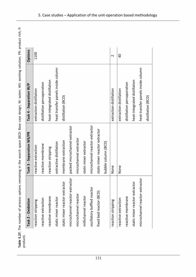
5. Case studies – Application of the unit-operation based methodology
131
Tabl
e 5.
27. T
he n
umbe
r of
pro
cess
opt
ions
rem
aini
ng in
the
sea
rch
spac
e (B
CD: B
ase
case
des
ign;
W: w
ater
; WS:
wor
king
sol
utio
n; P
R: p
rodu
ct r
ich;
P:
prod
uct).
Ta
sk 2
- O
xida
tion
Task
3 -
Sepa
ratio
n W
S/PR
Ta
sk 4
- Se
para
tion
W/P
O
ptio
ns
reac
tion
strip
ping
re
activ
e ex
trac
tion
extr
actio
n di
still
atio
n 11
00
reac
tive
extr
actio
n re
activ
e m
embr
ane
dist
illat
ion
perv
apor
atio
n
reac
tive
mem
bran
e re
actio
n st
rippi
ng
heat
-inte
grat
ed d
istill
atio
n
stat
ic m
ixer
reac
tor
extr
activ
e di
still
atio
n he
at tr
ansf
er p
anel
s ins
ide
colu
mn
stat
ic m
ixer
reac
tor e
xtra
ctor
m
embr
ane
extr
actio
n di
still
atio
n (B
CD)
mic
roch
anne
l rea
ctor
-ext
ract
or
pack
ed m
icro
chan
nel e
xtra
ctor
mic
roch
anne
l rea
ctor
m
icro
chan
nel e
xtra
ctor
mill
icha
nnel
reac
tor
stat
ic m
ixer
ext
ract
or
osci
llato
ry b
affle
d re
acto
r m
icro
chan
nel r
eact
or-e
xtra
ctor
fixed
bed
reac
tor (
BCD)
st
atic
mix
er re
acto
r ext
ract
or
bu
bble
colu
mn
(BCD
)
reac
tion
strip
ping
N
one
extr
actio
n di
still
atio
n 2
reac
tive
extr
actio
n N
one
extr
actio
n di
still
atio
n 40
reac
tive
mem
bran
e
dist
illat
ion
perv
apor
atio
n
stat
ic m
ixer
reac
tor e
xtra
ctor
heat
-inte
grat
ed d
istill
atio
n
mic
roch
anne
l rea
ctor
-ext
ract
or
he
at tr
ansf
er p
anel
s ins
ide
colu
mn
dist
illat
ion
(BCD
)
161
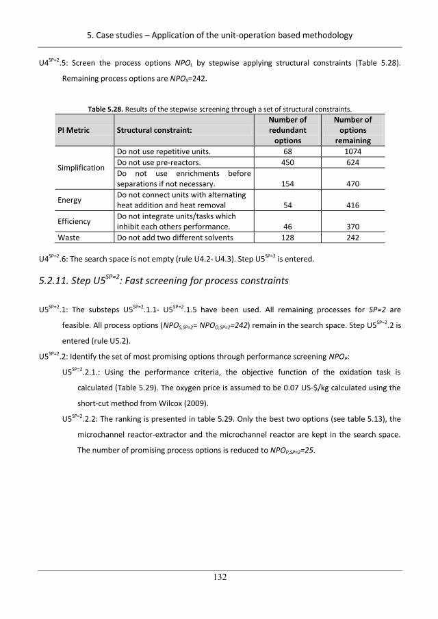
5. Case studies – Application of the unit-operation based methodology
132
U4SP=2.5: Screen the process options NPOL by stepwise applying structural constraints (Table 5.28).
Remaining process options are NPOS=242.
Table 5.28. Results of the stepwise screening through a set of structural constraints.
PI Metric Structural constraint: Number of redundant
options
Number of options
remaining
Simplification
Do not use repetitive units. 68 1074 Do not use pre-reactors. 450 624 Do not use enrichments before separations if not necessary. 154 470
Energy Do not connect units with alternating heat addition and heat removal 54 416
Efficiency Do not integrate units/tasks which inhibit each others performance. 46 370
Waste Do not add two different solvents 128 242 U4SP=2.6: The search space is not empty (rule U4.2- U4.3). Step U5SP=2 is entered.
5.2.11. Step U5SP=2: Fast screening for process constraints
U5SP=2.1: The substeps U5SP=2.1.1- U5SP=2.1.5 have been used. All remaining processes for SP=2 are
feasible. All process options (NPOS,SP=2= NPOO,SP=2=242) remain in the search space. Step U5SP=2.2 is
entered (rule U5.2).
U5SP=2.2: Identify the set of most promising options through performance screening NPOP:
U5SP=2.2.1.: Using the performance criteria, the objective function of the oxidation task is
calculated (Table 5.29). The oxygen price is assumed to be 0.07 US-$/kg calculated using the
short-cut method from Wilcox (2009).
U5SP=2.2.2: The ranking is presented in table 5.29. Only the best two options (see table 5.13), the
microchannel reactor-extractor and the microchannel reactor are kept in the search space.
The number of promising process options is reduced to NPOP,SP=2=25.
162
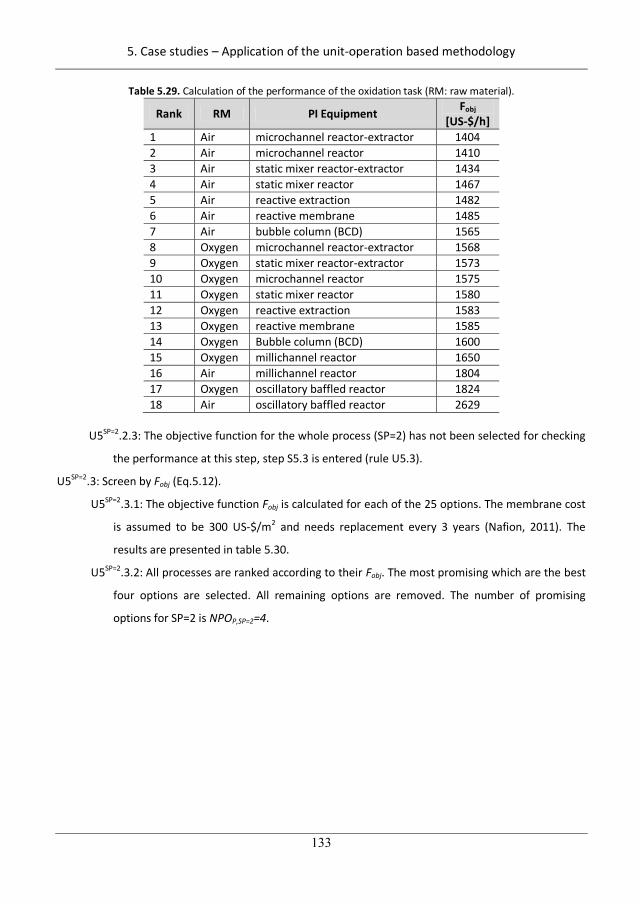
5. Case studies – Application of the unit-operation based methodology
133
Table 5.29. Calculation of the performance of the oxidation task (RM: raw material).
Rank RM PI Equipment Fobj [US-$/h]
1 Air microchannel reactor-extractor 1404 2 Air microchannel reactor 1410 3 Air static mixer reactor-extractor 1434 4 Air static mixer reactor 1467 5 Air reactive extraction 1482 6 Air reactive membrane 1485 7 Air bubble column (BCD) 1565 8 Oxygen microchannel reactor-extractor 1568 9 Oxygen static mixer reactor-extractor 1573 10 Oxygen microchannel reactor 1575 11 Oxygen static mixer reactor 1580 12 Oxygen reactive extraction 1583 13 Oxygen reactive membrane 1585 14 Oxygen Bubble column (BCD) 1600 15 Oxygen millichannel reactor 1650 16 Air millichannel reactor 1804 17 Oxygen oscillatory baffled reactor 1824 18 Air oscillatory baffled reactor 2629
U5SP=2.2.3: The objective function for the whole process (SP=2) has not been selected for checking
the performance at this step, step S5.3 is entered (rule U5.3).
U5SP=2.3: Screen by Fobj (Eq.5.12).
U5SP=2.3.1: The objective function Fobj is calculated for each of the 25 options. The membrane cost
is assumed to be 300 US-$/m2 and needs replacement every 3 years (Nafion, 2011). The
results are presented in table 5.30.
U5SP=2.3.2: All processes are ranked according to their Fobj. The most promising which are the best
four options are selected. All remaining options are removed. The number of promising
options for SP=2 is NPOP,SP=2=4.
163
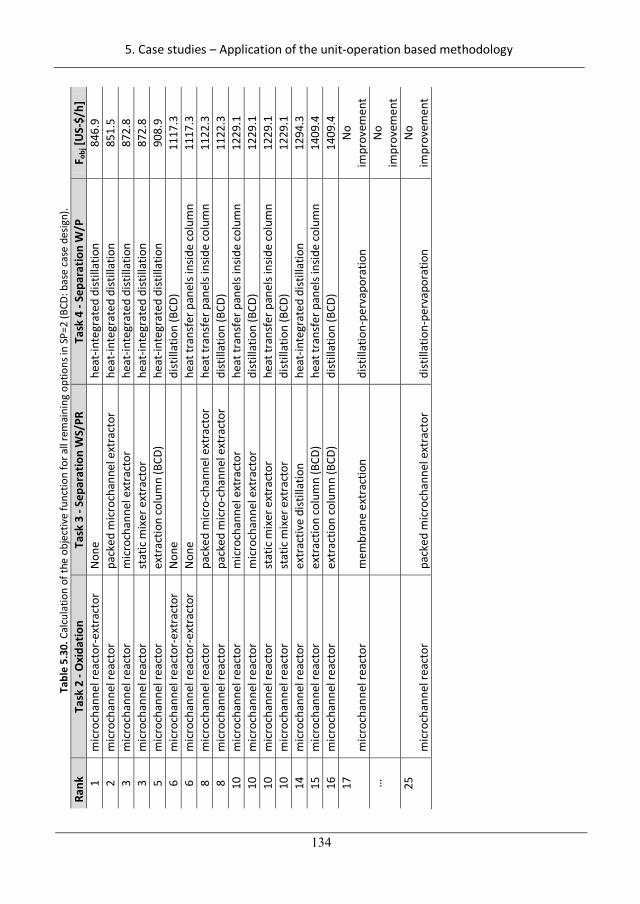
5. Case studies – Application of the unit-operation based methodology
134
Tabl
e 5.
30. C
alcu
latio
n of
the
obje
ctiv
e fu
nctio
n fo
r all
rem
aini
ng o
ptio
ns in
SP=
2 (B
CD: b
ase
case
des
ign)
. Ra
nk
Task
2 -
Oxi
datio
n Ta
sk 3
- Se
para
tion
WS/
PR
Task
4 -
Sepa
ratio
n W
/P
F obj
[US-
$/h]
1
mic
roch
anne
l rea
ctor
-ext
ract
or
Non
e he
at-in
tegr
ated
dist
illat
ion
846.
9 2
mic
roch
anne
l rea
ctor
pa
cked
mic
roch
anne
l ext
ract
or
heat
-inte
grat
ed d
istill
atio
n 85
1.5
3 m
icro
chan
nel r
eact
or
mic
roch
anne
l ext
ract
or
heat
-inte
grat
ed d
istill
atio
n 87
2.8
3 m
icro
chan
nel r
eact
or
stat
ic m
ixer
ext
ract
or
heat
-inte
grat
ed d
istill
atio
n 87
2.8
5 m
icro
chan
nel r
eact
or
extr
actio
n co
lum
n (B
CD)
heat
-inte
grat
ed d
istill
atio
n 90
8.9
6 m
icro
chan
nel r
eact
or-e
xtra
ctor
N
one
dist
illat
ion
(BCD
) 11
17.3
6
mic
roch
anne
l rea
ctor
-ext
ract
or
Non
e he
at tr
ansf
er p
anel
s ins
ide
colu
mn
1117
.3
8 m
icro
chan
nel r
eact
or
pack
ed m
icro
-cha
nnel
ext
ract
or
heat
tran
sfer
pan
els i
nsid
e co
lum
n 11
22.3
8
mic
roch
anne
l rea
ctor
pa
cked
mic
ro-c
hann
el e
xtra
ctor
di
still
atio
n (B
CD)
1122
.3
10
mic
roch
anne
l rea
ctor
m
icro
chan
nel e
xtra
ctor
he
at tr
ansf
er p
anel
s ins
ide
colu
mn
1229
.1
10
mic
roch
anne
l rea
ctor
m
icro
chan
nel e
xtra
ctor
di
still
atio
n (B
CD)
1229
.1
10
mic
roch
anne
l rea
ctor
st
atic
mix
er e
xtra
ctor
he
at tr
ansf
er p
anel
s ins
ide
colu
mn
1229
.1
10
mic
roch
anne
l rea
ctor
st
atic
mix
er e
xtra
ctor
di
still
atio
n (B
CD)
1229
.1
14
mic
roch
anne
l rea
ctor
ex
trac
tive
dist
illat
ion
heat
-inte
grat
ed d
istill
atio
n 12
94.3
15
m
icro
chan
nel r
eact
or
extr
actio
n co
lum
n (B
CD)
heat
tran
sfer
pan
els i
nsid
e co
lum
n 14
09.4
16
m
icro
chan
nel r
eact
or
extr
actio
n co
lum
n (B
CD)
dist
illat
ion
(BCD
) 14
09.4
17
m
icro
chan
nel r
eact
or
mem
bran
e ex
trac
tion
dist
illat
ion-
perv
apor
atio
n N
o im
prov
emen
t …
No
impr
ovem
ent
25
mic
roch
anne
l rea
ctor
pa
cked
mic
roch
anne
l ext
ract
or
dist
illat
ion-
perv
apor
atio
n N
o im
prov
emen
t
164
5. Case studies – Application of the unit-operation based methodology
135
U5SP=2.4: All sub-problems SP have been solved, step U5.5 is entered (Rule U5.4).
U5SP=2.5: All obtained solutions of each sub-problem SP are collected. The number of process options
remaining are NPOP=8. No additional logical and structural constraints as well as performance
criteria are selected. Hence, step U4.1-U4.5 are not needed and step 6 is entered.
5.2.12. Step 6: Solve the reduced optimization problem and validate promising
Step 6.1: Identify the set of most promising process options by solving an MINLP problem (if necessary).
Step 6.1.1: The search space NPOP=4·2=8<15. Hence, step 6.2 is entered.
Step 6.2: For each of the eight remaining process options, the mathematical model is optimized.
Temperatures and pressures in the reactors have been fixed leaving the volume (reaction time) as
the optimization variable. For the purification step, the pressure for purifying the product is fixed
to P=0.1 atm while reflux ratio and the pressure for the heat integration are the optimization
variables (Table 5.31). The reactors have been optimized separately using ICAS-MOT while the
optimization of the purification step has been made in Pro\II.
Step 6.3: All options are ranked by their objective function values. The best option (see Table 5.31) is the
hydrogenation in a microchannel reactor (catalyst on the wall) followed by a coupling of oxidation
and extraction in a microchannel reactor-extractor. The purification is realized in a heat integrated
distillation column (see Fig. 5.12).
Note: The key to the large process improvement is the energy savings in the purification as well as
the lower residence times in the microchannel reactors allowing less degradation of the product
and the solvents.
Step 6.4: The results have been obtained using the most detailed models. The distillation column has
been successfully rigorously validated in Pro\II (see Figure 5.12).
165
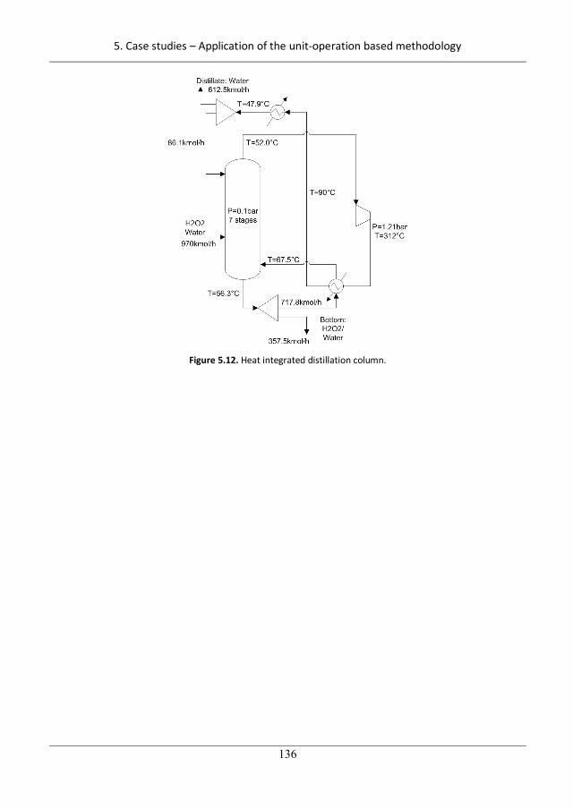
5. Case studies – Application of the unit-operation based methodology
136
Figure 5.12. Heat integrated distillation column.
166
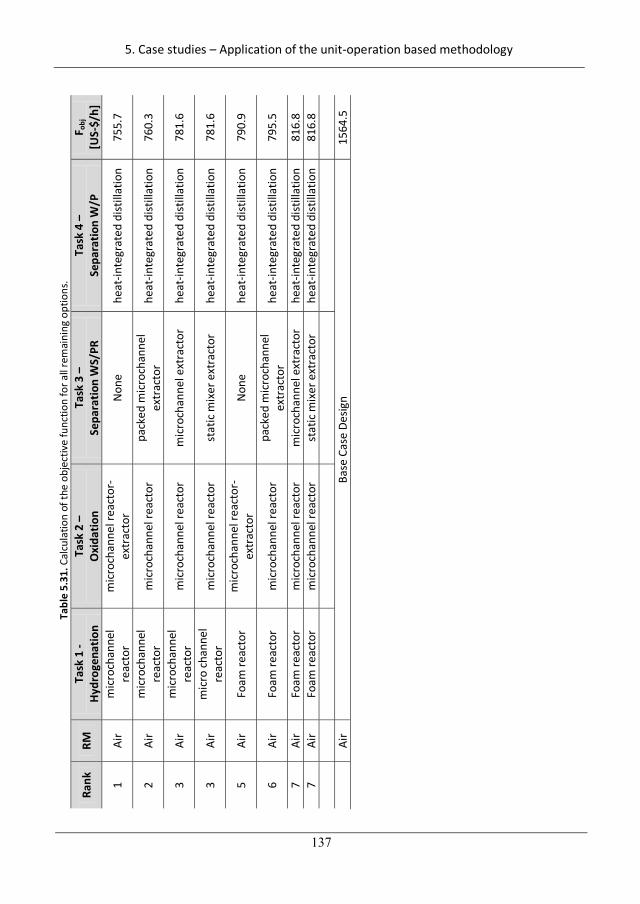
5. Case studies – Application of the unit-operation based methodology
137
Tabl
e 5.
31. C
alcu
latio
n of
the
obje
ctiv
e fu
nctio
n fo
r all
rem
aini
ng o
ptio
ns.
Rank
RM
Ta
sk 1
- Hy
drog
enat
ion
Task
2 –
O
xida
tion
Task
3 –
Se
para
tion
WS/
PR
Task
4 –
Se
para
tion
W/P
F o
bj
[US-
$/h]
1 Ai
r m
icro
chan
nel
reac
tor
mic
roch
anne
l rea
ctor
-ex
trac
tor
Non
e he
at-in
tegr
ated
dist
illat
ion
755.
7
2 Ai
r m
icro
chan
nel
reac
tor
mic
roch
anne
l rea
ctor
pa
cked
mic
roch
anne
l ex
trac
tor
heat
-inte
grat
ed d
istill
atio
n 76
0.3
3 Ai
r m
icro
chan
nel
reac
tor
mic
roch
anne
l rea
ctor
m
icro
chan
nel e
xtra
ctor
he
at-in
tegr
ated
dist
illat
ion
781.
6
3 Ai
r m
icro
chan
nel
reac
tor
mic
roch
anne
l rea
ctor
st
atic
mix
er e
xtra
ctor
he
at-in
tegr
ated
dist
illat
ion
781.
6
5 Ai
r Fo
am re
acto
r m
icro
chan
nel r
eact
or-
extr
acto
r N
one
heat
-inte
grat
ed d
istill
atio
n 79
0.9
6 Ai
r Fo
am re
acto
r m
icro
chan
nel r
eact
or
pack
ed m
icro
chan
nel
extr
acto
r he
at-in
tegr
ated
dist
illat
ion
795.
5
7 Ai
r Fo
am re
acto
r m
icro
chan
nel r
eact
or
mic
roch
anne
l ext
ract
or
heat
-inte
grat
ed d
istill
atio
n 81
6.8
7 Ai
r Fo
am re
acto
r m
icro
chan
nel r
eact
or
stat
ic m
ixer
ext
ract
or
heat
-inte
grat
ed d
istil
latio
n 81
6.8
Air
Base
Cas
e De
sign
1564
.5
167
5. Case studies – Application of the unit-operation based methodology
138
5.3. Production of HMF
For a sustainable future, biomass is considered as a renewable feedstock to replace oil in the chemical
industry. One example is the production of 5-hydroxymethylfurfural (HMF) from fructose. HMF is
considered as a platform chemical for the production of a variety of high value chemicals as well as high
value polymers (Bozell & Petersen, 2010). However, the production costs for HMF using this route and
conventional equipment are too high (Boisen et al., 2009). Therefore, it is checked if PI options can
reduce the operational costs of this process route. Section 5.3.1 lists the state-of-the-art in the bio-
based production of HMF from fructose; section 5.3.2 presents the base-case design while in steps
5.3.3-5.3.9 all details of the workflow (unit-operation) are presented.
5.3.1. State-of-the-art in the production of HMF
HMF can be produced from fructose by the following reaction scheme consisting of four reactions
proposed by Kuster and Temmink (1977). The main reaction is to produce HMF and water from fructose
(R1; Eq.5.33):
6 12 6 6 6 3 23C H O C H O H O . (5.33)
HMF is degraded in water to levulinic acid and formic acid in a side-reaction (R2; Eq.5.34).
6 6 3 2 5 8 3 2 22C H O H O C H O CH O (5.34)
Besides, two additional side-reactions are taking place to form humins which are the degradation of
HMF (R3; Eq.5.35) and the degradation of fructose (R4; Eq.5.36). Humins are undetermined insoluble
polymers (Rapp, 1977).
6 6 3 6 6 3 Humins.2C H O C H O (5.35)
6 12 6 6 6 3 2Humins.13C H O C H O H O (5.36)
Different process routes are discussed in academia and industry with respect to different catalysts,
different solvents (water, DMSO, ionic liquids) or mixture of solvents (e.g. water-acetone), and different
technologies for the reaction as well as the product recovery. An excellent review has been made by
Boisen et al. (2009). A small overview is given in Table 5.32. That also includes intensified technologies
such as reactive extraction to in-situ remove the product HMF (e.g. Román-Leshkov, Chheda & Dumesic,
2006) and circumvent the degradation of product and susbtrate; as well as ionic liquids replacing water
as solvent and acting as catalysts at the same time (e.g. in Moreau, Finiels & Vanoie, 2006).
168
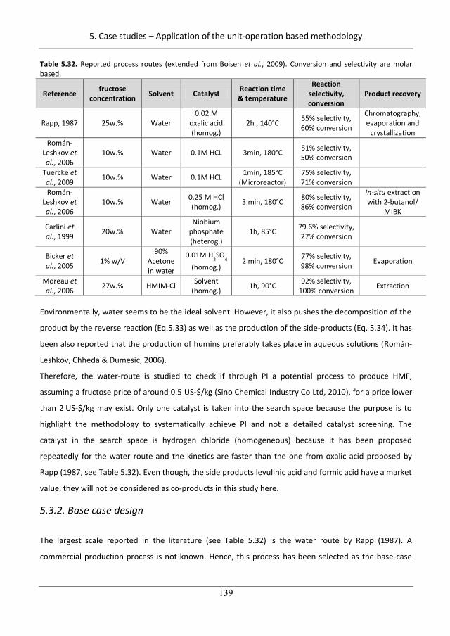
5. Case studies – Application of the unit-operation based methodology
139
Table 5.32. Reported process routes (extended from Boisen et al., 2009). Conversion and selectivity are molar based.
Reference fructose concentration Solvent Catalyst Reaction time
& temperature
Reaction selectivity, conversion
Product recovery
Rapp, 1987 25w.% Water 0.02 M
oxalic acid (homog.)
2h , 140°C 55% selectivity, 60% conversion
Chromatography, evaporation and
crystallization Román-
Leshkov et al., 2006
10w.% Water 0.1M HCL 3min, 180°C 51% selectivity, 50% conversion
Tuercke et al., 2009 10w.% Water 0.1M HCL 1min, 185°C
(Microreactor) 75% selectivity, 71% conversion
Román-Leshkov et al., 2006
10w.% Water 0.25 M HCl (homog.) 3 min, 180°C 80% selectivity,
86% conversion
In-situ extraction with 2-butanol/
MIBK
Carlini et al., 1999 20w.% Water
Niobium phosphate (heterog.)
1h, 85°C 79.6% selectivity, 27% conversion
Bicker et al., 2005 1% w/V
90% Acetone in water
0.01M H2SO
4 (homog.)
2 min, 180°C 77% selectivity, 98% conversion Evaporation
Moreau et al., 2006 27w.% HMIM-Cl Solvent
(homog.) 1h, 90°C 92% selectivity, 100% conversion Extraction
Environmentally, water seems to be the ideal solvent. However, it also pushes the decomposition of the
product by the reverse reaction (Eq.5.33) as well as the production of the side-products (Eq. 5.34). It has
been also reported that the production of humins preferably takes place in aqueous solutions (Román-
Leshkov, Chheda & Dumesic, 2006).
Therefore, the water-route is studied to check if through PI a potential process to produce HMF,
assuming a fructose price of around 0.5 US-$/kg (Sino Chemical Industry Co Ltd, 2010), for a price lower
than 2 US-$/kg may exist. Only one catalyst is taken into the search space because the purpose is to
highlight the methodology to systematically achieve PI and not a detailed catalyst screening. The
catalyst in the search space is hydrogen chloride (homogeneous) because it has been proposed
repeatedly for the water route and the kinetics are faster than the one from oxalic acid proposed by
Rapp (1987, see Table 5.32). Even though, the side products levulinic acid and formic acid have a market
value, they will not be considered as co-products in this study here.
5.3.2. Base case design
The largest scale reported in the literature (see Table 5.32) is the water route by Rapp (1987). A
commercial production process is not known. Hence, this process has been selected as the base-case
169
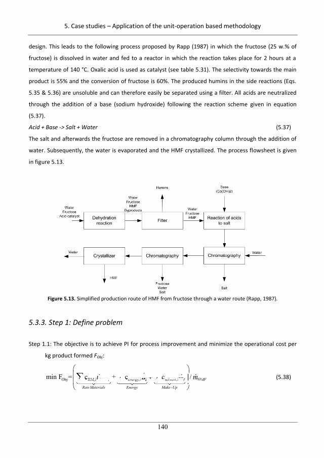
5. Case studies – Application of the unit-operation based methodology
140
design. This leads to the following process proposed by Rapp (1987) in which the fructose (25 w.% of
fructose) is dissolved in water and fed to a reactor in which the reaction takes place for 2 hours at a
temperature of 140 °C. Oxalic acid is used as catalyst (see table 5.31). The selectivity towards the main
product is 55% and the conversion of fructose is 60%. The produced humins in the side reactions (Eqs.
5.35 & 5.36) are unsoluble and can therefore easily be separated using a filter. All acids are neutralized
through the addition of a base (sodium hydroxide) following the reaction scheme given in equation
(5.37).
Acid + Base -> Salt + Water (5.37)
The salt and afterwards the fructose are removed in a chromatography column through the addition of
water. Subsequently, the water is evaporated and the HMF crystallized. The process flowsheet is given
in figure 5.13.
Figure 5.13. Simplified production route of HMF from fructose through a water route (Rapp, 1987).
5.3.3. Step 1: Define problem
Step 1.1: The objective is to achieve PI for process improvement and minimize the operational cost per
kg product formed FObj:
Obj RM,i , energy,i solvent,imin F = c + c c /RM i i i HMF
RawMaterials Make UpEnergy
m E m m/ MFm/i+ c+ c+ c+ c ii+ c+ c cc lc HMso ve , isolvent,iRM,i ,RM,i ,RM i ,, HM/ m//isolvent isolvent iisolvent ienergy ienergy ienergy i lle e gy,e e gy,e e gy,energy,ienergy,ienergy ienergy ienergy ienergy ienergy ienergy i (5.38)
170
5. Case studies – Application of the unit-operation based methodology
141
Step 1.2: The design scenario is to develop a new design of the whole process. The process scenario is
continuous.
Step 1.3: The product HMF is produced from the raw material fructose. All raw materials are pure and
the purity of the product is defined to be at least 95% (molar basis). The solvent of fructose is
water. The filtration of the humins is 100%. One catalyst is considered which is hydrogen chloride.
Step 1.4: Waste, efficiency, energy consumption, simplification.
Step 1.5: The maturity of the process is defined to be “medium”.
Step 1.6: Translate and PM into logical (Eq.2.2), structural (Eq.2.3), operational constraints (Eq.2.5)
and/or performance criteria (Eq.2.6):
Step 1.6.1: All rules have been applied to gather a set of logical constraints (Eq.2.2). The detailed
results are listed in Table 5.33.
Step 1.6.2: Four PI metrics have been translated to six structural constraints (see Table 5.12).
Step 1.6.3: The result of the translation into operational constraints (Eq.2.5) and the PI screening
criterion (Eq.2.6) is given in Table 5.33. The yield for screening in step 5 is defined as
, ,
100%HMF
Fructose reactor in
nn
(5.39)
Step 1.7: A base case design exists, step A2 is entered (rule 1.9).
171
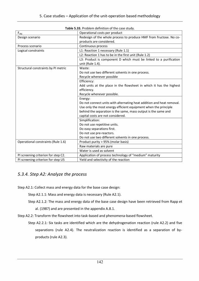
5. Case studies – Application of the unit-operation based methodology
142
Table 5.33. Problem definition of the case study. Fobj Operational costs per product Design scenario Redesign of the whole process to produce HMF from fructose. No co-
products are considered. Process scenario Continuous process Logical constraints L1: Reaction 1 necessary (Rule 1.1)
L2: Reaction 1 has to be in the first unit (Rule 1.2) L3: Product is component D which must be linked to a purification unit (Rule 1.4).
Structural constraints by PI metric Waste: Do not use two different solvents in one process. Recycle whenever possible Efficiency: Add units at the place in the flowsheet in which it has the highest efficiency. Recycle whenever possible. Energy: Do not connect units with alternating heat addition and heat removal. Use only the most energy efficient equipment when the principle behind the separation is the same, mass output is the same and capital costs are not considered. Simplification: Do not use repetitive units. Do easy separations first. Do not use pre-reactors. Do not use two different solvents in one process.
Operational constraints (Rule 1.6) Product purity > 95% (molar basis) Raw materials are pure Water is used as solvent
PI screening criterion for step C2. Application of process technology of “medium” maturity PI screening criterion for step U5 Yield and selectivity of the reaction
5.3.4. Step A2: Analyze the process
Step A2.1: Collect mass and energy data for the base case design:
Step A2.1.1: Mass and energy data is necessary (Rule A2.1).
Step A2.1.2: The mass and energy data of the base case design have been retrieved from Rapp et
al. (1987) and are presented in the appendix A.8.1.
Step A2.2: Transform the flowsheet into task-based and phenomena-based flowsheet.
Step A2.2.1: Six tasks are identified which are the dehydrogenation reaction (rule A2.2) and five
separations (rule A2.4). The neutralization reaction is identified as a separation of by-
products (rule A2.3).
172
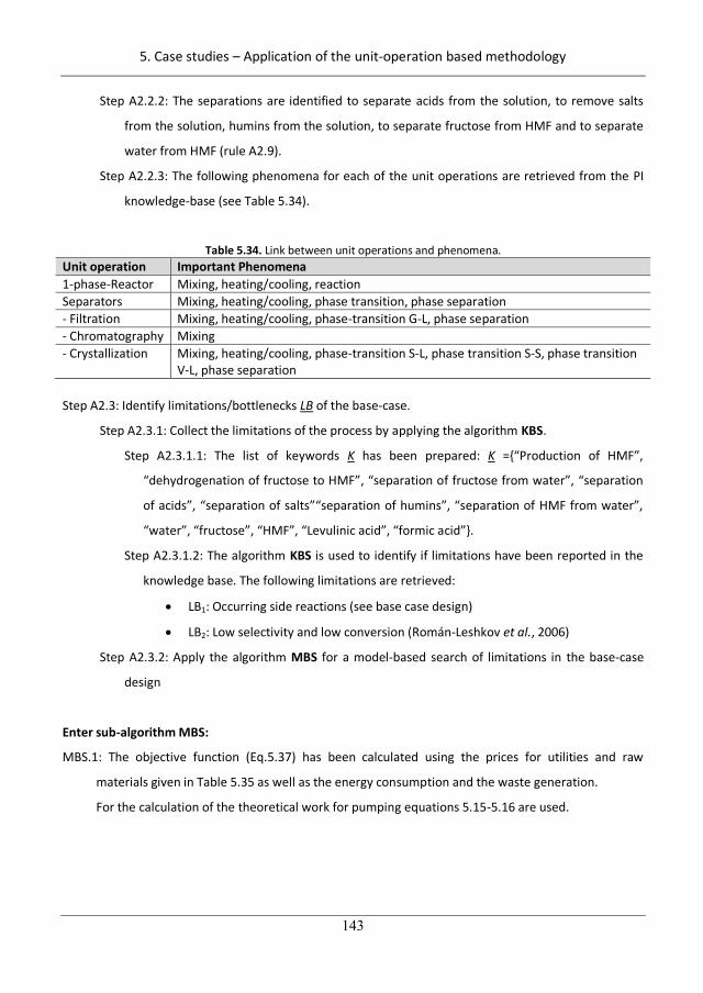
5. Case studies – Application of the unit-operation based methodology
143
Step A2.2.2: The separations are identified to separate acids from the solution, to remove salts
from the solution, humins from the solution, to separate fructose from HMF and to separate
water from HMF (rule A2.9).
Step A2.2.3: The following phenomena for each of the unit operations are retrieved from the PI
knowledge-base (see Table 5.34).
Table 5.34. Link between unit operations and phenomena. Unit operation Important Phenomena 1-phase-Reactor Mixing, heating/cooling, reaction Separators Mixing, heating/cooling, phase transition, phase separation - Filtration Mixing, heating/cooling, phase-transition G-L, phase separation - Chromatography Mixing - Crystallization Mixing, heating/cooling, phase-transition S-L, phase transition S-S, phase transition
V-L, phase separation Step A2.3: Identify limitations/bottlenecks LB of the base-case.
Step A2.3.1: Collect the limitations of the process by applying the algorithm KBS.
Step A2.3.1.1: The list of keywords K has been prepared: K ={“Production of HMF”,
“dehydrogenation of fructose to HMF”, “separation of fructose from water”, “separation
of acids”, “separation of salts”“separation of humins”, “separation of HMF from water”,
“water”, “fructose”, “HMF”, “Levulinic acid”, “formic acid”}.
Step A2.3.1.2: The algorithm KBS is used to identify if limitations have been reported in the
knowledge base. The following limitations are retrieved:
LB1: Occurring side reactions (see base case design)
LB2: Low selectivity and low conversion (Román-Leshkov et al., 2006)
Step A2.3.2: Apply the algorithm MBS for a model-based search of limitations in the base-case
design
Enter sub-algorithm MBS:
MBS.1: The objective function (Eq.5.37) has been calculated using the prices for utilities and raw
materials given in Table 5.35 as well as the energy consumption and the waste generation.
For the calculation of the theoretical work for pumping equations 5.15-5.16 are used.
173
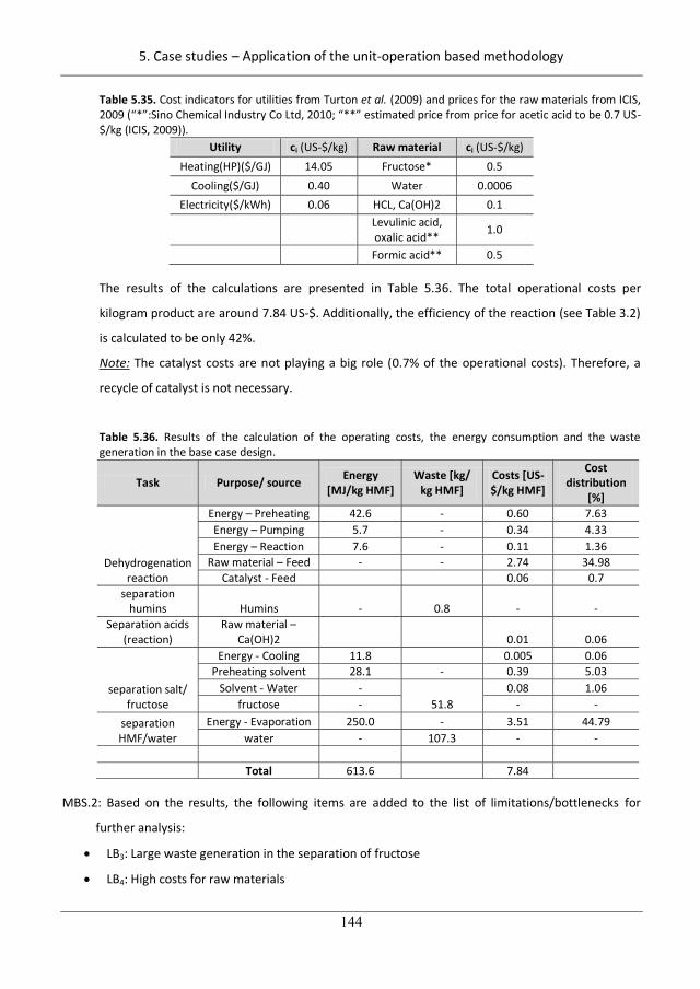
5. Case studies – Application of the unit-operation based methodology
144
Table 5.35. Cost indicators for utilities from Turton et al. (2009) and prices for the raw materials from ICIS, 2009 (“*”:Sino Chemical Industry Co Ltd, 2010; “**” estimated price from price for acetic acid to be 0.7 US-$/kg (ICIS, 2009)).
Utility ci (US-$/kg) Raw material ci (US-$/kg) Heating(HP)($/GJ) 14.05 Fructose* 0.5
Cooling($/GJ) 0.40 Water 0.0006 Electricity($/kWh) 0.06 HCL, Ca(OH)2 0.1
Levulinic acid, oxalic acid** 1.0
Formic acid** 0.5 The results of the calculations are presented in Table 5.36. The total operational costs per
kilogram product are around 7.84 US-$. Additionally, the efficiency of the reaction (see Table 3.2)
is calculated to be only 42%.
Note: The catalyst costs are not playing a big role (0.7% of the operational costs). Therefore, a
recycle of catalyst is not necessary.
Table 5.36. Results of the calculation of the operating costs, the energy consumption and the waste generation in the base case design.
Task Purpose/ source Energy [MJ/kg HMF]
Waste [kg/ kg HMF]
Costs [US-$/kg HMF]
Cost distribution
[%]
Dehydrogenation reaction
Energy – Preheating 42.6 - 0.60 7.63 Energy – Pumping 5.7 - 0.34 4.33 Energy – Reaction 7.6 - 0.11 1.36
Raw material – Feed - - 2.74 34.98 Catalyst - Feed 0.06 0.7
separation humins Humins - 0.8 - -
Separation acids (reaction)
Raw material – Ca(OH)2 0.01 0.06
separation salt/ fructose
Energy - Cooling 11.8 0.005 0.06 Preheating solvent 28.1 - 0.39 5.03
Solvent - Water - 51.8
0.08 1.06 fructose - - -
separation HMF/water
Energy - Evaporation 250.0 - 3.51 44.79 water - 107.3 - -
Total 613.6 7.84
MBS.2: Based on the results, the following items are added to the list of limitations/bottlenecks for
further analysis:
LB3: Large waste generation in the separation of fructose
LB4: High costs for raw materials
174
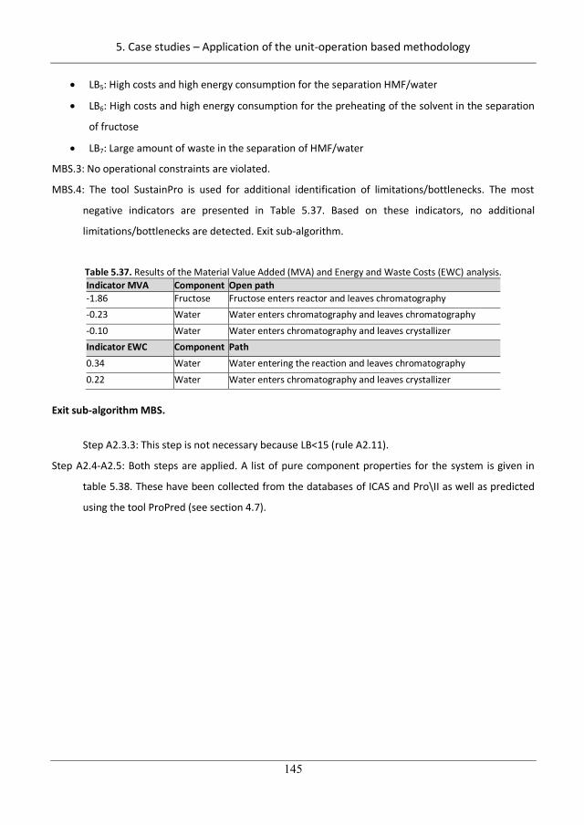
5. Case studies – Application of the unit-operation based methodology
145
LB5: High costs and high energy consumption for the separation HMF/water
LB6: High costs and high energy consumption for the preheating of the solvent in the separation
of fructose
LB7: Large amount of waste in the separation of HMF/water
MBS.3: No operational constraints are violated.
MBS.4: The tool SustainPro is used for additional identification of limitations/bottlenecks. The most
negative indicators are presented in Table 5.37. Based on these indicators, no additional
limitations/bottlenecks are detected. Exit sub-algorithm.
Table 5.37. Results of the Material Value Added (MVA) and Energy and Waste Costs (EWC) analysis. Indicator MVA Component Open path -1.86 Fructose Fructose enters reactor and leaves chromatography -0.23 Water Water enters chromatography and leaves chromatography -0.10 Water Water enters chromatography and leaves crystallizer Indicator EWC Component Path 0.34 Water Water entering the reaction and leaves chromatography 0.22 Water Water enters chromatography and leaves crystallizer
Exit sub-algorithm MBS.
Step A2.3.3: This step is not necessary because LB<15 (rule A2.11).
Step A2.4-A2.5: Both steps are applied. A list of pure component properties for the system is given in
table 5.38. These have been collected from the databases of ICAS and Pro\II as well as predicted
using the tool ProPred (see section 4.7).
175
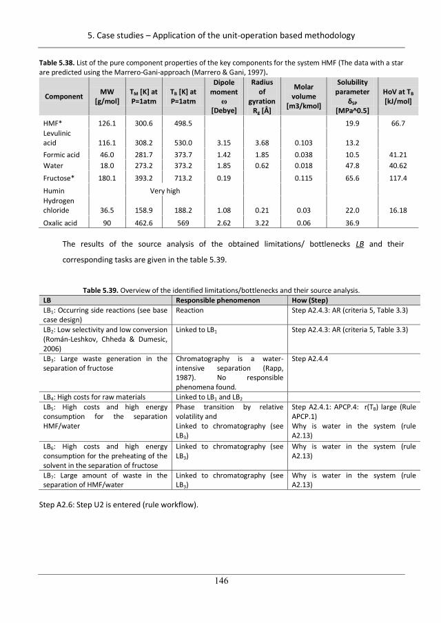
5. Case studies – Application of the unit-operation based methodology
146
Table 5.38. List of the pure component properties of the key components for the system HMF (The data with a star are predicted using the Marrero-Gani-approach (Marrero & Gani, 1997).
Component MW [g/mol]
TM [K] at P=1atm
TB [K] at P=1atm
Dipole moment
[Debye]
Radius of
gyration Rg [Å]
Molar volume
[m3/kmol]
Solubility parameter
SP [MPa^0.5]
HoV at TB [kJ/mol]
HMF* 126.1 300.6 498.5 19.9 66.7 Levulinic acid 116.1 308.2 530.0 3.15 3.68 0.103 13.2 Formic acid 46.0 281.7 373.7 1.42 1.85 0.038 10.5 41.21 Water 18.0 273.2 373.2 1.85 0.62 0.018 47.8 40.62
Fructose* 180.1 393.2 713.2 0.19 0.115 65.6 117.4
Humin Very high Hydrogen chloride 36.5 158.9 188.2 1.08 0.21 0.03 22.0 16.18
Oxalic acid 90 462.6 569 2.62 3.22 0.06 36.9
The results of the source analysis of the obtained limitations/ bottlenecks LB and their
corresponding tasks are given in the table 5.39.
Table 5.39. Overview of the identified limitations/bottlenecks and their source analysis. LB Responsible phenomenon How (Step) LB1: Occurring side reactions (see base case design)
Reaction Step A2.4.3: AR (criteria 5, Table 3.3)
LB2: Low selectivity and low conversion (Román-Leshkov, Chheda & Dumesic, 2006)
Linked to LB1 Step A2.4.3: AR (criteria 5, Table 3.3)
LB3: Large waste generation in the separation of fructose
Chromatography is a water-intensive separation (Rapp, 1987). No responsible phenomena found.
Step A2.4.4
LB4: High costs for raw materials Linked to LB1 and LB2 LB5: High costs and high energy consumption for the separation HMF/water
Phase transition by relative volatility and Linked to chromatography (see LB3)
Step A2.4.1: APCP.4: r(TB) large (Rule APCP.1) Why is water in the system (rule A2.13)
LB6: High costs and high energy consumption for the preheating of the solvent in the separation of fructose
Linked to chromatography (see LB3)
Why is water in the system (rule A2.13)
LB7: Large amount of waste in the separation of HMF/water
Linked to chromatography (see LB3)
Why is water in the system (rule A2.13)
Step A2.6: Step U2 is entered (rule workflow).
176
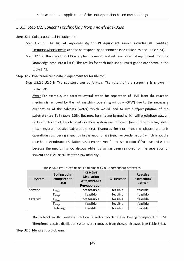
5. Case studies – Application of the unit-operation based methodology
147
5.3.5. Step U2: Collect PI technology from Knowledge-Base
Step U2.1: Collect potential PI equipment:
Step U2.1.1: The list of keywords KPI for PI equipment search includes all identified
limitations/bottlenecks and the corresponding phenomena (see Table 5.39 and Table 5.34).
Step U2.1.2: The algorithm KBS is applied to search and retrieve potential equipment from the
knowledge base into a list . The results for each task under investigation are shown in the
table 5.41.
Step U2.2: Pre-screen candidate PI equipment for feasibility:
Step U2.2.1-U2.2.4: The sub-steps are performed. The result of the screening is shown in
table 5.40.
Note: For example, the reactive crystallization for separation of HMF from the reaction
medium is removed by the not matching operating window (OPW) due to the necessary
evaporation of the solvents (water) which would lead to dry out/precipitation of the
substrate (see TB in table 5.38). Because, humins are formed which will precipitate out, all
units which cannot handle solids in their system are removed (membrane reactor, static
mixer reactor, reactive adsorption, etc). Examples for not matching phases are unit
operations considering a reaction in the vapor phase (reactive condensation) which is not the
case here. Membrane distillation has been removed for the separation of fructose and water
because the medium is too viscous while it also has been removed for the separation of
solvent and HMF because of the low maturity.
Table 5.40. Pre-Screening of PI equipment by pure component properties.
System Boiling point compared to
HMF
Reactive Distillation
with/without Pervaporation
All Reactor Reactive
extraction/ settler
Solvent TB,low not feasible feasible feasible TB,high feasible feasible feasible
Catalyst TB,low not feasible feasible feasible TB,high feasible feasible feasible Heterog. feasible feasible feasible
The solvent in the working solution is water which is low boiling compared to HMF.
Therefore, reactive distillation systems are removed from the search space (see Table 5.41).
Step U2.3: Identify sub-problems:
177

5. Case studies – Application of the unit-operation based methodology
148
Step U2.3.1: No sub-problems (SP=1) are identified (rule U2.4).
Step U2.3.2: All candidate PI equipment (see table 5.41) is put into the list .
Step U2.3.3: Enter the inner algorithm for the sub-problem SP=1 (step U3).
178
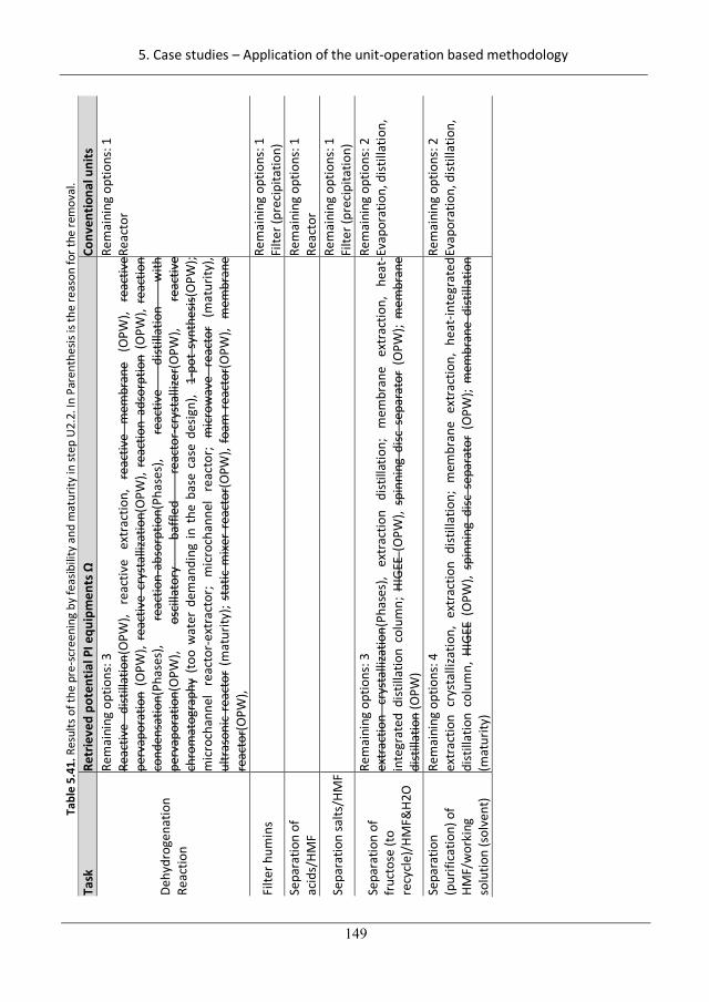
5. Case studies – Application of the unit-operation based methodology
149
Tabl
e 5.
41. R
esul
ts o
f the
pre
-scr
eeni
ng b
y fe
asib
ility
and
mat
urity
in st
ep U
2.2.
In P
aren
thes
is is
the
reas
on fo
r the
rem
oval
. Ta
sk
Retr
ieve
d po
tent
ial P
I equ
ipm
ents
Conv
entio
nal u
nits
Dehy
drog
enat
ion
Reac
tion
Rem
aini
ng o
ptio
ns: 3
Re
activ
e di
still
atio
n (O
PW),
reac
tive
extr
actio
n,
reac
tive
mem
bran
e (O
PW),
reac
tive
perv
apor
atio
n (O
PW),
reac
tive
crys
talli
zatio
n(O
PW),
reac
tion
adso
rptio
n (O
PW),
reac
tion
cond
ensa
tion(
Phas
es),
reac
tion-
abso
rptio
n(Ph
ases
), re
activ
e di
still
atio
n w
ith
perv
apor
atio
n(O
PW),
osci
llato
ry
baffl
ed
reac
tor-
crys
talli
zer(
OPW
), re
activ
e ch
rom
atog
raph
y (to
o w
ater
dem
andi
ng in
the
bas
e ca
se d
esig
n),
1-po
t sy
nthe
sis(O
PW);
mic
roch
anne
l re
acto
r-ex
trac
tor;
mic
roch
anne
l re
acto
r; m
icro
wav
e re
acto
r (m
atur
ity),
ultr
ason
ic r
eact
or (
mat
urity
); st
atic
mix
er r
eact
or(O
PW),
foam
rea
ctor
(OPW
), m
embr
ane
reac
tor(
OPW
),
Rem
aini
ng o
ptio
ns: 1
Re
acto
r
Filte
r hum
ins
Re
mai
ning
opt
ions
: 1
Filte
r (pr
ecip
itatio
n)
Sepa
ratio
n of
ac
ids/
HMF
Re
mai
ning
opt
ions
: 1
Reac
tor
Sepa
ratio
n sa
lts/H
MF
Re
mai
ning
opt
ions
: 1
Filte
r (pr
ecip
itatio
n)
Sepa
ratio
n of
fr
ucto
se (t
o re
cycl
e)/H
MF&
H2O
Rem
aini
ng o
ptio
ns: 3
ex
trac
tion
crys
talli
zatio
n(Ph
ases
), ex
trac
tion
dist
illat
ion;
m
embr
ane
extr
actio
n,
heat
-in
tegr
ated
dist
illat
ion
colu
mn;
HIG
EE (
OPW
), sp
inni
ng d
isc s
epar
ator
(O
PW);
mem
bran
e di
still
atio
n (O
PW)
Rem
aini
ng o
ptio
ns: 2
Ev
apor
atio
n, d
istill
atio
n,
Sepa
ratio
n (p
urifi
catio
n) o
f HM
F/w
orki
ng
solu
tion
(sol
vent
)
Rem
aini
ng o
ptio
ns: 4
ex
trac
tion
crys
talli
zatio
n, e
xtra
ctio
n di
still
atio
n; m
embr
ane
extr
actio
n, h
eat-
inte
grat
ed
dist
illat
ion
colu
mn,
HIG
EE (
OPW
), sp
inni
ng d
isc s
epar
ator
(O
PW);
mem
bran
e di
still
atio
n (m
atur
ity)
Rem
aini
ng o
ptio
ns: 2
Ev
apor
atio
n, d
istill
atio
n,
179
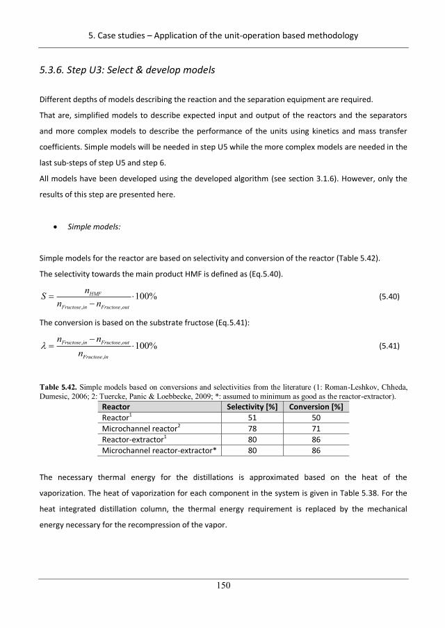
5. Case studies – Application of the unit-operation based methodology
150
5.3.6. Step U3: Select & develop models
Different depths of models describing the reaction and the separation equipment are required.
That are, simplified models to describe expected input and output of the reactors and the separators
and more complex models to describe the performance of the units using kinetics and mass transfer
coefficients. Simple models will be needed in step U5 while the more complex models are needed in the
last sub-steps of step U5 and step 6.
All models have been developed using the developed algorithm (see section 3.1.6). However, only the
results of this step are presented here.
Simple models:
Simple models for the reactor are based on selectivity and conversion of the reactor (Table 5.42).
The selectivity towards the main product HMF is defined as (Eq.5.40).
, ,
100%HMF
Fructose in Fructose out
nSn n
(5.40)
The conversion is based on the substrate fructose (Eq.5.41):
, ,
,
100%Fructose in Fructose out
Fructose in
n nn
(5.41)
Table 5.42. Simple models based on conversions and selectivities from the literature (1: Roman-Leshkov, Chheda, Dumesic, 2006; 2: Tuercke, Panic & Loebbecke, 2009; *: assumed to minimum as good as the reactor-extractor).
Reactor Selectivity [%] Conversion [%] Reactor1 51 50 Microchannel reactor2 78 71 Reactor-extractor1 80 86 Microchannel reactor-extractor* 80 86
The necessary thermal energy for the distillations is approximated based on the heat of the
vaporization. The heat of vaporization for each component in the system is given in Table 5.38. For the
heat integrated distillation column, the thermal energy requirement is replaced by the mechanical
energy necessary for the recompression of the vapor.
180
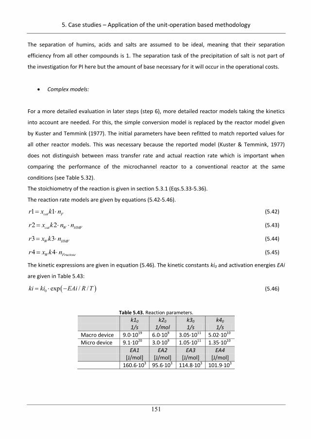
5. Case studies – Application of the unit-operation based methodology
151
The separation of humins, acids and salts are assumed to be ideal, meaning that their separation
efficiency from all other compounds is 1. The separation task of the precipitation of salt is not part of
the investigation for PI here but the amount of base necessary for it will occur in the operational costs.
Complex models:
For a more detailed evaluation in later steps (step 6), more detailed reactor models taking the kinetics
into account are needed. For this, the simple conversion model is replaced by the reactor model given
by Kuster and Temmink (1977). The initial parameters have been refitted to match reported values for
all other reactor models. This was necessary because the reported model (Kuster & Temmink, 1977)
does not distinguish between mass transfer rate and actual reaction rate which is important when
comparing the performance of the microchannel reactor to a conventional reactor at the same
conditions (see Table 5.32).
The stoichiometry of the reaction is given in section 5.3.1 (Eqs.5.33-5.36).
The reaction rate models are given by equations (5.42-5.46).
1 1cat Fr x k n (5.42)
2 2cat W HMFr x k n n (5.43)
3 3W HMFr x k n (5.44)
4 4W Fructoser x k n (5.45)
The kinetic expressions are given in equation (5.46). The kinetic constants ki0 and activation energies EAi
are given in Table 5.43:
0 exp / /ki ki EAi R T (5.46)
Table 5.43. Reaction parameters. k10 k20 k30 k40 1/s 1/mol 1/s 1/s
Macro device 9.0·1019 6.0·109 3.05·1011 5.02·1010 Micro device 9.1·1020 3.0·109 1.05·1011 1.35·1010
EA1 EA2 EA3 EA4 [J/mol] [J/mol] [J/mol] [J/mol]
160.6·103 95.6·103 114.8·103 101.9·103
181
5. Case studies – Application of the unit-operation based methodology
152
Besides the reaction, also the extraction needs to be modeled. The phase transition of HMF by
extraction is modeled using equation 5.47.
,12 , , ,HMF L HMF aq HMF aq HMF orgn k a n x R x (5.47)
It is assumed that through proper solvent selection, other components will not enter the solvent phase
because of an existing difference in the solubility parameter between the compounds (Table 5.38).
The following parameters are needed to model the extraction units: the solvent dependent partition
coefficient R (Eq.5.48); the equipment dependent contact area between the phases a; as well as the
mass transfer coefficient KL assumed to be independent of equipment and solvent (Eq.5.49).
The partition coefficient is:
, ,/HMF org HMF aqR x x (5.48)
The mass transfer coefficient has been calculated using the kinetic and extraction model for the solvent
7:3 MIBK:2-butanol for the data given by Roman-Leshkov et al. (2006). The mass transfer coefficient is: 24.85 10 /Lk m s (5.49)
The value of kLa enhanced for different PI equipment is shown in Table 5.25. These factors have been
used to distinguish between reactive-extraction in a column and in a micro device (enhancement factor
E=18 for the micro device).
The partition coefficient is known for three different solvents (Roman-Leshkov & Dumesic, 2009). Based
on these and the corresponding Hildebrandt’s solubility parameters of the solvents and HMF, the
behavior of unknown solvents with HMF is predicted. This is shown in the appendix A.8.3.
The loss of solvent to water is directly modeled using the predicted values for the water solubility for
new solvent, retrieved from ProPred (see section 4).
5.3.7. Step U4: Generate feasible flowsheet options
U4.1: The superstructure containing a generic model has been retrieved from the model library (see
Fig.4.2).
U4.2: This step is not needed, since the superstructure from S4.1 matches the maximum number of
tasks, therefore step U4SP=1.3 is directly entered (Rule U4.1).
U4.3: The number of options represented by this superstructure is calculated using (Eq.5.8).
The number of identified units is NIU=16. The number of processing steps is four, assuming that
the removal of acids and humins is ideal and merged into one task. Therefore the total number of
generated options assuming only one solvent/membrane is:
182
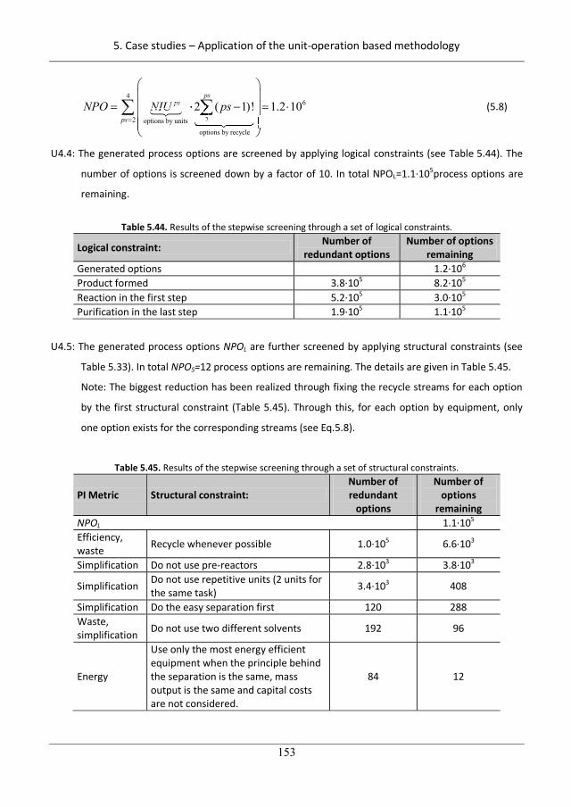
5. Case studies – Application of the unit-operation based methodology
153
46
2 2options by unitsoptions by recycle
2 ( 1)! 1.2 10ps
ps
psNPO NIU psNIU 22NIU psNIU 2p
22
(5.8)
U4.4: The generated process options are screened by applying logical constraints (see Table 5.44). The
number of options is screened down by a factor of 10. In total NPOL=1.1·105process options are
remaining.
Table 5.44. Results of the stepwise screening through a set of logical constraints.
Logical constraint: Number of redundant options
Number of options remaining
Generated options 1.2·106 Product formed 3.8·105 8.2·105 Reaction in the first step 5.2·105 3.0·105 Purification in the last step 1.9·105 1.1·105
U4.5: The generated process options NPOL are further screened by applying structural constraints (see
Table 5.33). In total NPOS=12 process options are remaining. The details are given in Table 5.45.
Note: The biggest reduction has been realized through fixing the recycle streams for each option
by the first structural constraint (Table 5.45). Through this, for each option by equipment, only
one option exists for the corresponding streams (see Eq.5.8).
Table 5.45. Results of the stepwise screening through a set of structural constraints.
PI Metric Structural constraint: Number of redundant
options
Number of options
remaining NPOL 1.1·105 Efficiency, waste Recycle whenever possible 1.0·105 6.6·103
Simplification Do not use pre-reactors 2.8·103 3.8·103
Simplification Do not use repetitive units (2 units for the same task) 3.4·103 408
Simplification Do the easy separation first 120 288 Waste, simplification Do not use two different solvents 192 96
Energy
Use only the most energy efficient equipment when the principle behind the separation is the same, mass output is the same and capital costs are not considered.
84 12
183
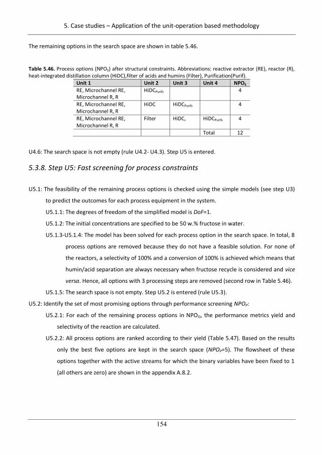
5. Case studies – Application of the unit-operation based methodology
154
The remaining options in the search space are shown in table 5.46.
Table 5.46. Process options (NPOS) after structural constraints. Abbreviations: reactive extractor (RE), reactor (R), heat-integrated distillation column (HiDC),filter of acids and humins (Filter), Purification(Purif).
Unit 1 Unit 2 Unit 3 Unit 4 NPOS
RE, Microchannel RE, Microchannel R, R
HiDCPurif, 4
RE, Microchannel RE, Microchannel R, R
HiDC HiDCPurif, 4
RE, Microchannel RE, Microchannel R, R
Filter HiDC, HiDCPurif, 4
Total 12
U4.6: The search space is not empty (rule U4.2- U4.3). Step U5 is entered.
5.3.8. Step U5: Fast screening for process constraints
U5.1: The feasibility of the remaining process options is checked using the simple models (see step U3)
to predict the outcomes for each process equipment in the system.
U5.1.1: The degrees of freedom of the simplified model is DoF=1.
U5.1.2: The initial concentrations are specified to be 50 w.% fructose in water.
U5.1.3-U5.1.4: The model has been solved for each process option in the search space. In total, 8
process options are removed because they do not have a feasible solution. For none of
the reactors, a selectivity of 100% and a conversion of 100% is achieved which means that
humin/acid separation are always necessary when fructose recycle is considered and vice
versa. Hence, all options with 3 processing steps are removed (second row in Table 5.46).
U5.1.5: The search space is not empty. Step U5.2 is entered (rule U5.3).
U5.2: Identify the set of most promising options through performance screening NPOP:
U5.2.1: For each of the remaining process options in NPOO, the performance metrics yield and
selectivity of the reaction are calculated.
U5.2.2: All process options are ranked according to their yield (Table 5.47). Based on the results
only the best five options are kept in the search space (NPOP=5). The flowsheet of these
options together with the active streams for which the binary variables have been fixed to 1
(all others are zero) are shown in the appendix A.8.2.
184
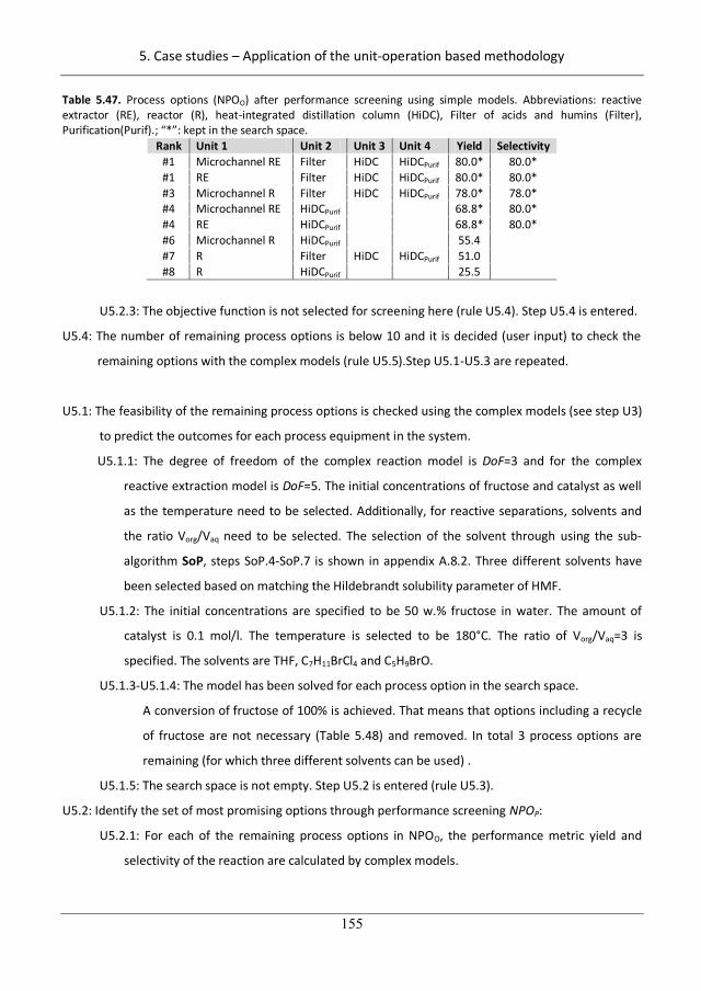
5. Case studies – Application of the unit-operation based methodology
155
Table 5.47. Process options (NPOO) after performance screening using simple models. Abbreviations: reactive extractor (RE), reactor (R), heat-integrated distillation column (HiDC), Filter of acids and humins (Filter), Purification(Purif).; “*”: kept in the search space.
Rank Unit 1 Unit 2 Unit 3 Unit 4 Yield Selectivity #1 Microchannel RE Filter HiDC HiDCPurif 80.0* 80.0* #1 RE Filter HiDC HiDCPurif 80.0* 80.0* #3 Microchannel R Filter HiDC HiDCPurif 78.0* 78.0* #4 Microchannel RE HiDCPurif 68.8* 80.0* #4 RE HiDCPurif 68.8* 80.0* #6 Microchannel R HiDCPurif 55.4 #7 R Filter HiDC HiDCPurif 51.0 #8 R HiDCPurif 25.5
U5.2.3: The objective function is not selected for screening here (rule U5.4). Step U5.4 is entered.
U5.4: The number of remaining process options is below 10 and it is decided (user input) to check the
remaining options with the complex models (rule U5.5).Step U5.1-U5.3 are repeated.
U5.1: The feasibility of the remaining process options is checked using the complex models (see step U3)
to predict the outcomes for each process equipment in the system.
U5.1.1: The degree of freedom of the complex reaction model is DoF=3 and for the complex
reactive extraction model is DoF=5. The initial concentrations of fructose and catalyst as well
as the temperature need to be selected. Additionally, for reactive separations, solvents and
the ratio Vorg/Vaq need to be selected. The selection of the solvent through using the sub-
algorithm SoP, steps SoP.4-SoP.7 is shown in appendix A.8.2. Three different solvents have
been selected based on matching the Hildebrandt solubility parameter of HMF.
U5.1.2: The initial concentrations are specified to be 50 w.% fructose in water. The amount of
catalyst is 0.1 mol/l. The temperature is selected to be 180°C. The ratio of Vorg/Vaq=3 is
specified. The solvents are THF, C7H11BrCl4 and C5H9BrO.
U5.1.3-U5.1.4: The model has been solved for each process option in the search space.
A conversion of fructose of 100% is achieved. That means that options including a recycle
of fructose are not necessary (Table 5.48) and removed. In total 3 process options are
remaining (for which three different solvents can be used) .
U5.1.5: The search space is not empty. Step U5.2 is entered (rule U5.3).
U5.2: Identify the set of most promising options through performance screening NPOP:
U5.2.1: For each of the remaining process options in NPOO, the performance metric yield and
selectivity of the reaction are calculated by complex models.
185
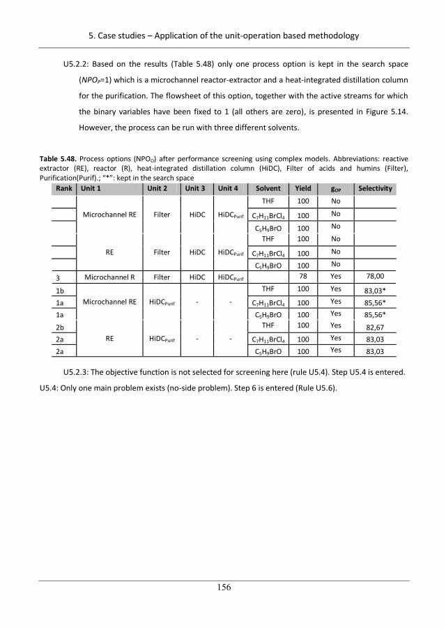
5. Case studies – Application of the unit-operation based methodology
156
U5.2.2: Based on the results (Table 5.48) only one process option is kept in the search space
(NPOP=1) which is a microchannel reactor-extractor and a heat-integrated distillation column
for the purification. The flowsheet of this option, together with the active streams for which
the binary variables have been fixed to 1 (all others are zero), is presented in Figure 5.14.
However, the process can be run with three different solvents.
Table 5.48. Process options (NPOO) after performance screening using complex models. Abbreviations: reactive extractor (RE), reactor (R), heat-integrated distillation column (HiDC), Filter of acids and humins (Filter), Purification(Purif).; “*”: kept in the search space
Rank Unit 1 Unit 2 Unit 3 Unit 4 Solvent Yield gOP Selectivity
Microchannel RE Filter HiDC HiDCPurif
THF 100 No C7H11BrCl4 100 No C5H9BrO 100 No
RE Filter HiDC HiDCPurif
THF 100 No C7H11BrCl4 100 No
C5H9BrO 100 No 3 Microchannel R Filter HiDC HiDCPurif 78 Yes 78,00
1b Microchannel RE HiDCPurif - -
THF 100 Yes 83,03* 1a C7H11BrCl4 100 Yes 85,56* 1a C5H9BrO 100 Yes 85,56*
2b RE HiDCPurif - -
THF 100 Yes 82,67 2a C7H11BrCl4 100 Yes 83,03 2a C5H9BrO 100 Yes 83,03
U5.2.3: The objective function is not selected for screening here (rule U5.4). Step U5.4 is entered.
U5.4: Only one main problem exists (no-side problem). Step 6 is entered (Rule U5.6).
186
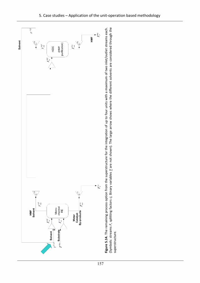
5. Case studies – Application of the unit-operation based methodology
157
Fi
gure
5.1
4. T
he re
mai
ning
pro
cess
opt
ion
from
the
supe
rstr
uctu
re fo
r the
inte
grat
ion
of u
p to
four
uni
ts w
ith a
max
imum
of t
wo
inle
t/ou
tlet s
trea
ms
each
. (S
ymbo
ls: s
trea
ms
F, s
plitt
ing
fact
ors
; Bin
ary
varia
bles
Y a
re n
ot s
how
n). T
he la
rge
arro
w s
how
s w
here
the
diffe
rent
sol
vent
s ar
e co
nsid
ered
thro
ugh
the
supe
rstr
uctu
re.
187
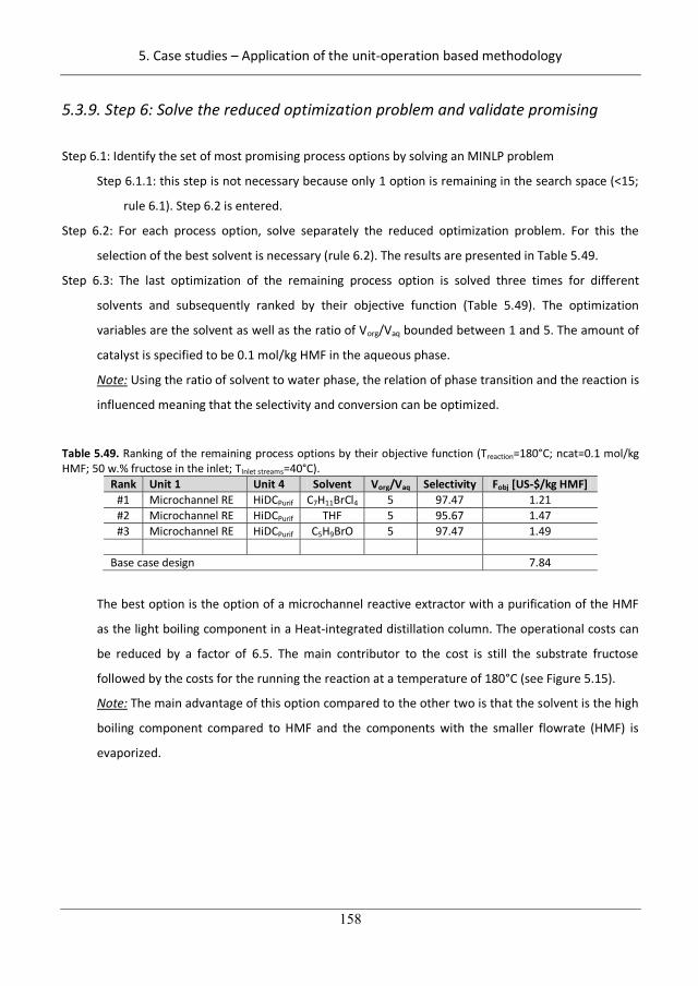
5. Case studies – Application of the unit-operation based methodology
158
5.3.9. Step 6: Solve the reduced optimization problem and validate promising
Step 6.1: Identify the set of most promising process options by solving an MINLP problem
Step 6.1.1: this step is not necessary because only 1 option is remaining in the search space (<15;
rule 6.1). Step 6.2 is entered.
Step 6.2: For each process option, solve separately the reduced optimization problem. For this the
selection of the best solvent is necessary (rule 6.2). The results are presented in Table 5.49.
Step 6.3: The last optimization of the remaining process option is solved three times for different
solvents and subsequently ranked by their objective function (Table 5.49). The optimization
variables are the solvent as well as the ratio of Vorg/Vaq bounded between 1 and 5. The amount of
catalyst is specified to be 0.1 mol/kg HMF in the aqueous phase.
Note: Using the ratio of solvent to water phase, the relation of phase transition and the reaction is
influenced meaning that the selectivity and conversion can be optimized.
Table 5.49. Ranking of the remaining process options by their objective function (Treaction=180°C; ncat=0.1 mol/kg HMF; 50 w.% fructose in the inlet; TInlet streams=40°C).
Rank Unit 1 Unit 4 Solvent Vorg/Vaq Selectivity Fobj [US-$/kg HMF] #1 Microchannel RE HiDCPurif C7H11BrCl4 5 97.47 1.21 #2 Microchannel RE HiDCPurif THF 5 95.67 1.47 #3 Microchannel RE HiDCPurif C5H9BrO 5 97.47 1.49
Base case design 7.84
The best option is the option of a microchannel reactive extractor with a purification of the HMF
as the light boiling component in a Heat-integrated distillation column. The operational costs can
be reduced by a factor of 6.5. The main contributor to the cost is still the substrate fructose
followed by the costs for the running the reaction at a temperature of 180°C (see Figure 5.15).
Note: The main advantage of this option compared to the other two is that the solvent is the high
boiling component compared to HMF and the components with the smaller flowrate (HMF) is
evaporized.
188
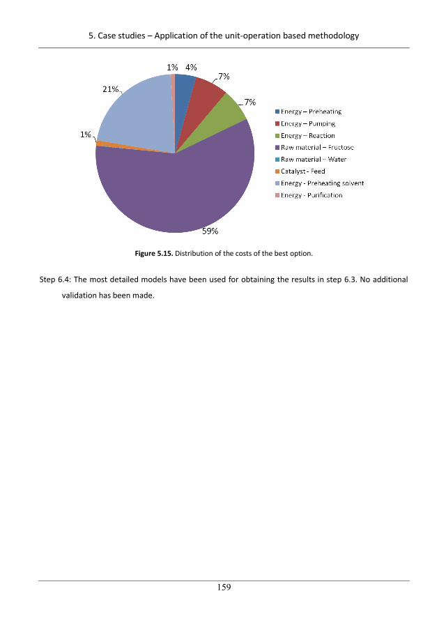
5. Case studies – Application of the unit-operation based methodology
159
Figure 5.15. Distribution of the costs of the best option.
Step 6.4: The most detailed models have been used for obtaining the results in step 6.3. No additional
validation has been made.
189

5. Case studies – Application of the unit-operation based methodology
160
190
6. Case studies – Application of the phenomena based methodology
161
Chapter 6.
Case studies – Application of the phenomena based methodology
The application of the methodology using the phenomena based workflow is highlighted through three
case studies: The first case study is the production of isopropyl-acetate from isopropanol and water. The
second case study is the separation of a bulk chemical hydrogen-peroxide from water which takes place
in the last step of the hydrogen-peroxide process via the anthraquinone route (see section 5.2). The
third case study highlights the application of the phenomena based methodology for the production of
cyclohexyl-acetate from cyclohexene and confirms that the existing PI solutions for this process can be
systematically generated and are part of the generated search space here.
6.1. Production of isopropyl-acetate
The application of the methodology is highlighted through the production of isopropyl acetate (IPAc)
which is shown in detail in sections 6.1.2.-6.1.7. Additional information is given in appendix A.9.
This case study has been selected for two reasons. First of all, isopropyl-acetate is an important bulk
chemical product used widely as organic solvent and process improvement with respect to operational
costs by PI is of high interest (Lai et al., 2007). Secondly, PI for esterification reactions (and especially
esterification of alcohol with acetic acid) have been widely studied before, mostly considering reactive
distillation (Lutze et al., 2010b). Comparisons to other PI equipment have not been found. Since reactive
distillation has been widely considered to intensify the process (e.g. Tang et al., 2005; Lai et al., 2007),
their design is checked against the performance of the outcome of the phenomena-based methodology
at the end of this section (section 6.1.8). In this case study, only the reaction task is targeted by PI.
6.1.1. Base-Case Design
Isopropyl-acetate can be produced by a reaction of acetic acid (HOAc) and isopropanol (IPOH) to form
isopropyl-acetate and as side-product water (H2O). The stoichimetry of the reaction is given in equation
(6.1) and takes place in the liquid phase. The reaction is catalyzed by a heterogeneous catalyst which is
Amberlyst 15 (Tang et al., 2005).
191
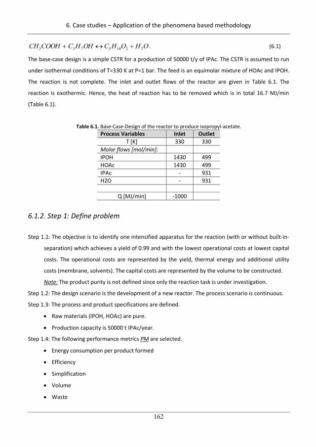
6. Case studies – Application of the phenomena based methodology
162
OHOHCOHHCCOOHCH 22105733 . (6.1)
The base-case design is a simple CSTR for a production of 50000 t/y of IPAc. The CSTR is assumed to run
under isothermal conditions of T=330 K at P=1 bar. The feed is an equimolar mixture of HOAc and IPOH.
The reaction is not complete. The inlet and outlet flows of the reactor are given in Table 6.1. The
reaction is exothermic. Hence, the heat of reaction has to be removed which is in total 16.7 MJ/min
(Table 6.1).
Table 6.1. Base-Case-Design of the reactor to produce isopropyl-acetate. Process Variables Inlet Outlet
T [K] 330 330 Molar flows [mol/min]: IPOH 1430 499 HOAc 1430 499 IPAc - 931 H2O - 931
Q [MJ/min] -1000
6.1.2. Step 1: Define problem
Step 1.1: The objective is to identify one intensified apparatus for the reaction (with or without built-in-
separation) which achieves a yield of 0.99 and with the lowest operational costs at lowest capital
costs. The operational costs are represented by the yield, thermal energy and additional utility
costs (membrane, solvents). The capital costs are represented by the volume to be constructed.
Note: The product purity is not defined since only the reaction task is under investigation.
Step 1.2: The design scenario is the development of a new reactor. The process scenario is continuous.
Step 1.3: The process and product specifications are defined.
Raw materials (IPOH, HOAc) are pure.
Production capacity is 50000 t IPAc/year.
Step 1.4: The following performance metrics PM are selected.
Energy consumption per product formed
Efficiency
Simplification
Volume
Waste
192
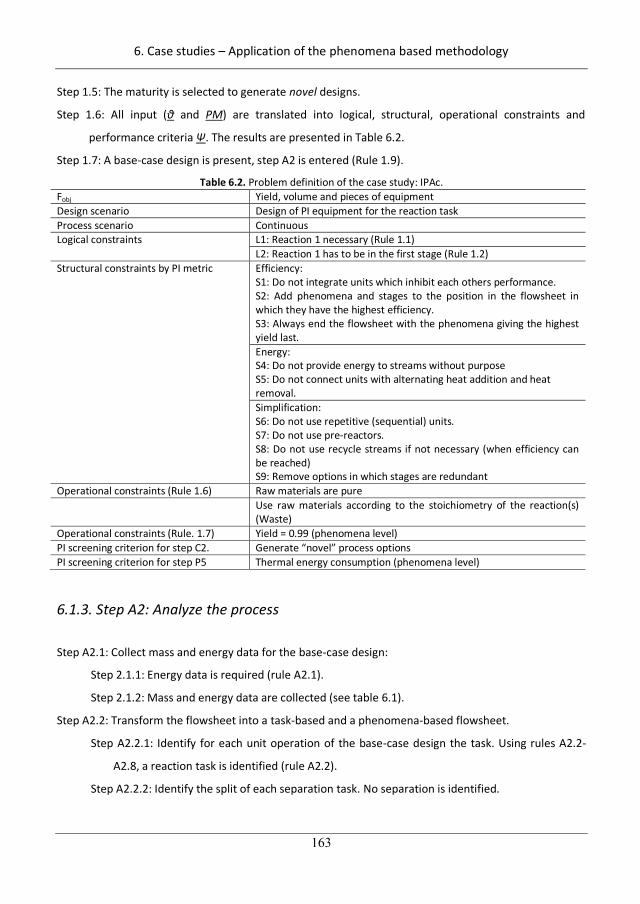
6. Case studies – Application of the phenomena based methodology
163
Step 1.5: The maturity is selected to generate novel designs.
Step 1.6: All input ( and PM) are translated into logical, structural, operational constraints and
performance criteria . The results are presented in Table 6.2.
Step 1.7: A base-case design is present, step A2 is entered (Rule 1.9).
Table 6.2. Problem definition of the case study: IPAc. Fobj Yield, volume and pieces of equipment Design scenario Design of PI equipment for the reaction task Process scenario Continuous Logical constraints L1: Reaction 1 necessary (Rule 1.1)
L2: Reaction 1 has to be in the first stage (Rule 1.2) Structural constraints by PI metric Efficiency:
S1: Do not integrate units which inhibit each others performance. S2: Add phenomena and stages to the position in the flowsheet in which they have the highest efficiency. S3: Always end the flowsheet with the phenomena giving the highest yield last. Energy: S4: Do not provide energy to streams without purpose S5: Do not connect units with alternating heat addition and heat removal. Simplification: S6: Do not use repetitive (sequential) units. S7: Do not use pre-reactors. S8: Do not use recycle streams if not necessary (when efficiency can be reached) S9: Remove options in which stages are redundant
Operational constraints (Rule 1.6) Raw materials are pure Use raw materials according to the stoichiometry of the reaction(s)
(Waste) Operational constraints (Rule. 1.7) Yield = 0.99 (phenomena level) PI screening criterion for step C2. Generate “novel” process options PI screening criterion for step P5 Thermal energy consumption (phenomena level)
6.1.3. Step A2: Analyze the process
Step A2.1: Collect mass and energy data for the base-case design:
Step 2.1.1: Energy data is required (rule A2.1).
Step 2.1.2: Mass and energy data are collected (see table 6.1).
Step A2.2: Transform the flowsheet into a task-based and a phenomena-based flowsheet.
Step A2.2.1: Identify for each unit operation of the base-case design the task. Using rules A2.2-
A2.8, a reaction task is identified (rule A2.2).
Step A2.2.2: Identify the split of each separation task. No separation is identified.
193
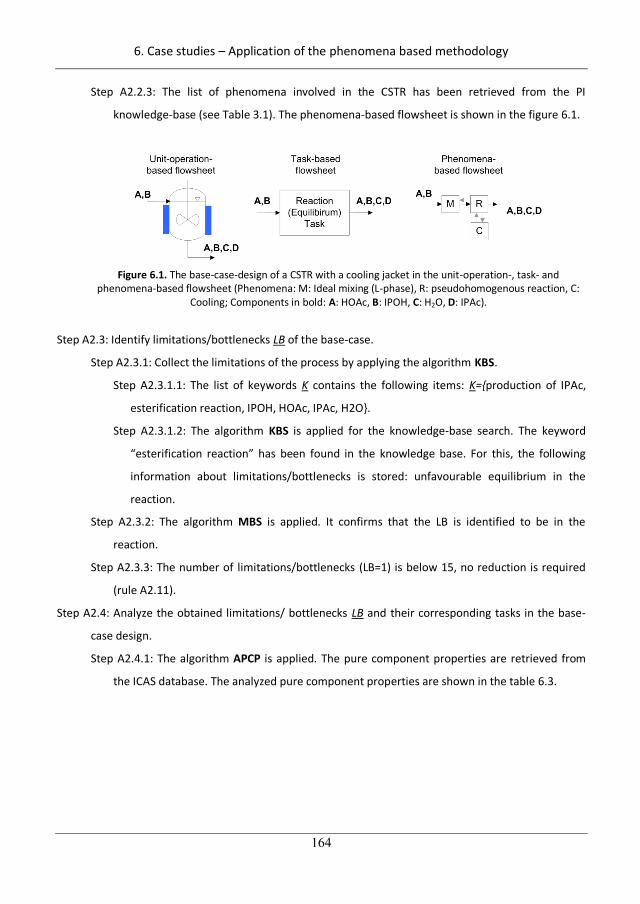
6. Case studies – Application of the phenomena based methodology
164
Step A2.2.3: The list of phenomena involved in the CSTR has been retrieved from the PI
knowledge-base (see Table 3.1). The phenomena-based flowsheet is shown in the figure 6.1.
Figure 6.1. The base-case-design of a CSTR with a cooling jacket in the unit-operation-, task- and
phenomena-based flowsheet (Phenomena: M: Ideal mixing (L-phase), R: pseudohomogenous reaction, C: Cooling; Components in bold: A: HOAc, B: IPOH, C: H2O, D: IPAc).
Step A2.3: Identify limitations/bottlenecks LB of the base-case.
Step A2.3.1: Collect the limitations of the process by applying the algorithm KBS.
Step A2.3.1.1: The list of keywords K contains the following items: K={production of IPAc,
esterification reaction, IPOH, HOAc, IPAc, H2O}.
Step A2.3.1.2: The algorithm KBS is applied for the knowledge-base search. The keyword
“esterification reaction” has been found in the knowledge base. For this, the following
information about limitations/bottlenecks is stored: unfavourable equilibrium in the
reaction.
Step A2.3.2: The algorithm MBS is applied. It confirms that the LB is identified to be in the
reaction.
Step A2.3.3: The number of limitations/bottlenecks (LB=1) is below 15, no reduction is required
(rule A2.11).
Step A2.4: Analyze the obtained limitations/ bottlenecks LB and their corresponding tasks in the base-
case design.
Step A2.4.1: The algorithm APCP is applied. The pure component properties are retrieved from
the ICAS database. The analyzed pure component properties are shown in the table 6.3.
194
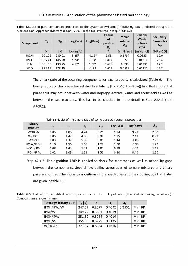
6. Case studies – Application of the phenomena based methodology
165
Table 6.3. List of pure component properties of the system at P=1 atm (“*”:Missing data predicted through the Marrero-Gani-Approach (Marrero & Gani, 2001) in the tool ProPred in step APCP.1.2).
Component TB TM Log (Ws) Log(Kow)
Radius of
gyration Rg
Molar volume
VM
Van der Waals
volume VdW
Solubility Parameter
SP
[K] [K] log(mg/L) [Å] [m³/kmol] [m³/kmol] [MPa^0.5] HOAc 391.05 289.91 5.25* -0.15* 2.61 0.1797 0.0333 19.0 IPOH 355.41 185.28 5.24* 0.53* 2.807 0.22 0.04216 23.4 IPAc 361.65 199.75 4.17* 1.32* 3.679 0.336 0.06299 17.2 H2O 373.15 273.15 -1.38 0.615 0.0559 0.01237 47.8
The binary ratio of the occurring components for each property is calculated (Table 6.4). The
binary ratio’s of the properties related to solubility (Log (Ws), Log(Kow)) hint that a potential
phase split may occur between water and isopropyl-acetate, water and acetic-acid as well as
between the two reactants. This has to be checked in more detail in Step A2.4.2 (rule
APCP.2).
Table 6.4. List of the binary ratio of some pure components properties. Binary
mixture TB TM Rg VM Log (Ws) Log(Kow) SP
W/HOAc 1.05 1.06 4.24 3.21 1.14 9.20 2.52 W/IPOH 1.05 1.47 4.56 3.94 1.15 2.49 0.73 W/IPAc 1.03 1.37 5.98 6.01 1.44 -1.05 2.79
HOAc/IPOH 1.10 1.56 1.08 1.22 1.00 -3.53 1.23 HOAc/IPAc 1.08 1.45 1.41 1.87 0.79 -0.11 1.11 IPOH/IPAc 1.02 1.08 1.31 1.53 0.80 0.40 1.36
Step A2.4.2: The algorithm AMP is applied to check for azeotropes as well as miscibility gaps
between the components. Several low boiling azeotropes of ternary mixtures and binary
pairs are formed. The molar compositions of the azeotropes and their boiling point at 1 atm
are given in table 6.5.
Table 6.5. List of the identified azeotropes in the mixture at p=1 atm (Min.BP=Low boiling azeotrope). Compositions are given in mol.
Ternary/ Binary pair TB [K] x1 x2 x3 IPOH/IPAc/W 347.37 0.2377 0.4092 0.3531 Min. BP IPAc/W 349.72 0.5981 0.4019 Min. BP IPOH/IPAc 351.69 0.5984 0.4016 Min. BP IPOH/W 355.65 0.6875 0.3125 Min. BP W/HOAc 371.97 0.8384 0.1616 Min. BP
195
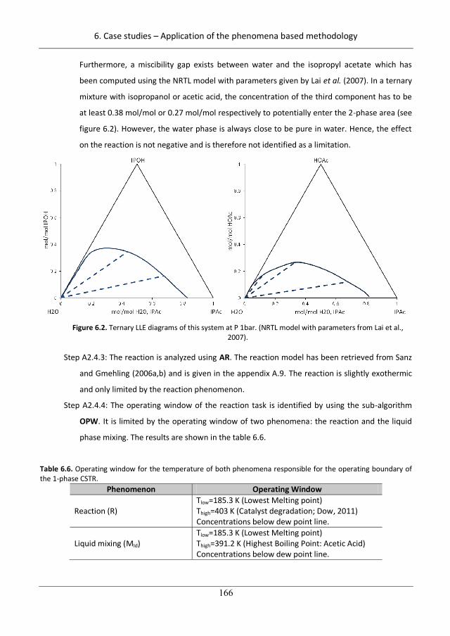
6. Case studies – Application of the phenomena based methodology
166
Furthermore, a miscibility gap exists between water and the isopropyl acetate which has
been computed using the NRTL model with parameters given by Lai et al. (2007). In a ternary
mixture with isopropanol or acetic acid, the concentration of the third component has to be
at least 0.38 mol/mol or 0.27 mol/mol respectively to potentially enter the 2-phase area (see
figure 6.2). However, the water phase is always close to be pure in water. Hence, the effect
on the reaction is not negative and is therefore not identified as a limitation.
Figure 6.2. Ternary LLE diagrams of this system at P 1bar. (NRTL model with parameters from Lai et al.,
2007).
Step A2.4.3: The reaction is analyzed using AR. The reaction model has been retrieved from Sanz
and Gmehling (2006a,b) and is given in the appendix A.9. The reaction is slightly exothermic
and only limited by the reaction phenomenon.
Step A2.4.4: The operating window of the reaction task is identified by using the sub-algorithm
OPW. It is limited by the operating window of two phenomena: the reaction and the liquid
phase mixing. The results are shown in the table 6.6.
Table 6.6. Operating window for the temperature of both phenomena responsible for the operating boundary of the 1-phase CSTR.
Phenomenon Operating Window
Reaction (R) Tlow=185.3 K (Lowest Melting point) Thigh=403 K (Catalyst degradation; Dow, 2011) Concentrations below dew point line.
Liquid mixing (MId) Tlow=185.3 K (Lowest Melting point) Thigh=391.2 K (Highest Boiling Point: Acetic Acid) Concentrations below dew point line.
196
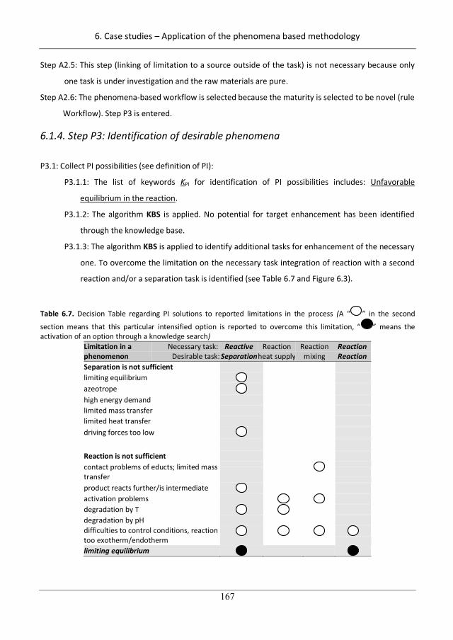
6. Case studies – Application of the phenomena based methodology
167
Step A2.5: This step (linking of limitation to a source outside of the task) is not necessary because only
one task is under investigation and the raw materials are pure.
Step A2.6: The phenomena-based workflow is selected because the maturity is selected to be novel (rule
Workflow). Step P3 is entered.
6.1.4. Step P3: Identification of desirable phenomena
P3.1: Collect PI possibilities (see definition of PI):
P3.1.1: The list of keywords KPI for identification of PI possibilities includes: Unfavorable
equilibrium in the reaction.
P3.1.2: The algorithm KBS is applied. No potential for target enhancement has been identified
through the knowledge base.
P3.1.3: The algorithm KBS is applied to identify additional tasks for enhancement of the necessary
one. To overcome the limitation on the necessary task integration of reaction with a second
reaction and/or a separation task is identified (see Table 6.7 and Figure 6.3).
Table 6.7. Decision Table regarding PI solutions to reported limitations in the process (A “ ” in the second
section means that this particular intensified option is reported to overcome this limitation, “ ” means the activation of an option through a knowledge search)
Limitation in a phenomenon
Necessary task: Desirable task:
Reactive Separation
Reaction heat supply
Reaction mixing
Reaction Reaction
Separation is not sufficient limiting equilibrium azeotrope high energy demand limited mass transfer limited heat transfer driving forces too low Reaction is not sufficient contact problems of educts; limited mass transfer
product reacts further/is intermediate activation problems degradation by T degradation by pH difficulties to control conditions, reaction too exotherm/endotherm
limiting equilibrium
197
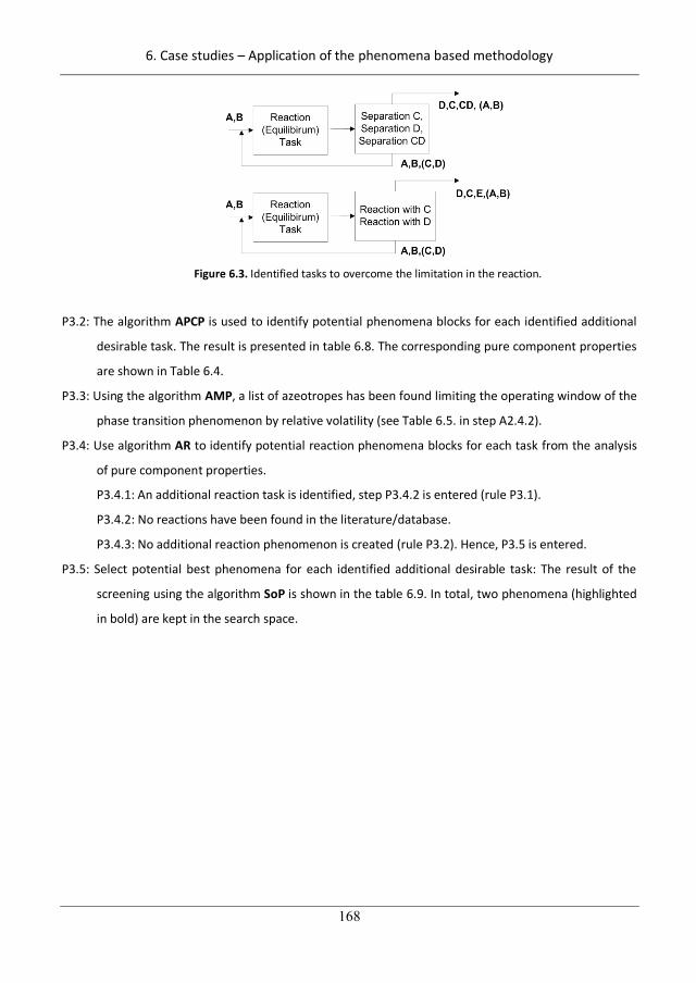
6. Case studies – Application of the phenomena based methodology
168
Figure 6.3. Identified tasks to overcome the limitation in the reaction.
P3.2: The algorithm APCP is used to identify potential phenomena blocks for each identified additional
desirable task. The result is presented in table 6.8. The corresponding pure component properties
are shown in Table 6.4.
P3.3: Using the algorithm AMP, a list of azeotropes has been found limiting the operating window of the
phase transition phenomenon by relative volatility (see Table 6.5. in step A2.4.2).
P3.4: Use algorithm AR to identify potential reaction phenomena blocks for each task from the analysis
of pure component properties.
P3.4.1: An additional reaction task is identified, step P3.4.2 is entered (rule P3.1).
P3.4.2: No reactions have been found in the literature/database.
P3.4.3: No additional reaction phenomenon is created (rule P3.2). Hence, P3.5 is entered.
P3.5: Select potential best phenomena for each identified additional desirable task: The result of the
screening using the algorithm SoP is shown in the table 6.9. In total, two phenomena (highlighted
in bold) are kept in the search space.
198
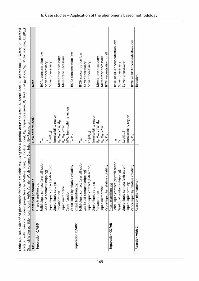
6. Case studies – Application of the phenomena based methodology
169
Tabl
e 6.
8. T
able
Iden
tifie
d ph
enom
ena
for
each
des
irabl
e ta
sk u
sing
the
algo
rithm
APC
P an
d AM
P (A
: Ace
tic-A
cid,
B: I
sopr
opan
ol, C
: Wat
er, D
: Iso
prop
yl-
acet
ate)
with
pur
e co
mpo
nent
pro
pert
ies
(TM
: Mel
ting
poin
t; T B
: Boi
ling
poin
t; P L
V: Va
por
pres
sure
; Rg:
Radi
us o
f gy
ratio
n; V
M: M
olar
vol
ume;
Log
(Kow
): O
ctan
ol/W
ater
par
titio
n co
effic
ient
; VdW
: Van
der
Waa
ls vo
lum
e;
SP: S
olub
ility
Par
amet
er)
Task
Id
entif
ied
phen
omen
a H
ow d
eter
min
ed?
Not
e Se
para
tion
C/AB
D Ph
ase
tran
sitio
n by
: So
lid-L
iqui
d co
ntac
t (cr
ysta
lliza
tion)
G
as-li
quid
con
tact
(str
ippi
ng)
Liqu
id-li
quid
con
tact
(ext
ract
ion)
Li
quid
-liqu
id se
ttlin
g Pe
rvap
orat
ion
Liqu
id m
embr
ane
Cent
rifug
atio
n Va
por-
liqui
d by
rela
tive
vola
tility
T M,
T B
Log(
K ow
) Im
misc
ibili
ty re
gion
R g
, VM
, VdW
, SP
R g
, VM
, VdW
M
W, I
mm
iscib
ility
regi
on
T B, P
LV
HOAc
con
cent
ratio
n lo
w
Solv
ent n
eces
sary
So
lven
t nec
essa
ry
Mem
bran
e ne
cess
ary
Mem
bran
e ne
cess
ary
HOAc
con
cent
ratio
n lo
w
Sepa
ratio
n D/
ABC
Phas
e tr
ansit
ion
by:
Solid
-Liq
uid
cont
act (
crys
talli
zatio
n)
Gas
-liqu
id c
onta
ct (s
trip
ping
) Li
quid
-liqu
id c
onta
ct (e
xtra
ctio
n)
Liqu
id-li
quid
sett
ling
Perv
apor
atio
n Li
quid
mem
bran
e Va
por-
liqui
d by
rela
tive
vola
tility
T M,
T B
Log(
K ow
) Im
misc
ibili
ty re
gion
R g
, VM
, VdW
, SP
R g
, VM
, VdW
T B
, PLV
IPO
H co
ncen
trat
ion
low
So
lven
t nec
essa
ry
Solv
ent n
eces
sary
M
embr
ane
nece
ssar
y M
embr
ane
nece
ssar
y IP
OH
once
ntra
tion
smal
l Se
para
tion
CD/A
B Ph
ase
tran
sitio
n by
: So
lid-L
iqui
d co
ntac
t (cr
ysta
lliza
tion)
G
as-li
quid
con
tact
(str
ippi
ng)
Liqu
id-li
quid
con
tact
(ext
ract
ion)
Li
quid
-liqu
id se
ttlin
g Va
por-
liqui
d by
rela
tive
vola
tility
T M,
T B
Log(
K ow
) Im
misc
ibili
ty re
gion
T B
, PLV
IPO
H or
HO
Ac c
once
ntra
tion
low
So
lven
t nec
essa
ry
Solv
ent n
eces
sary
IP
OH
or H
OAc
con
cent
ratio
n lo
w
Reac
tion
with
C
Reac
tion
phen
omen
on
Re
actio
n
199
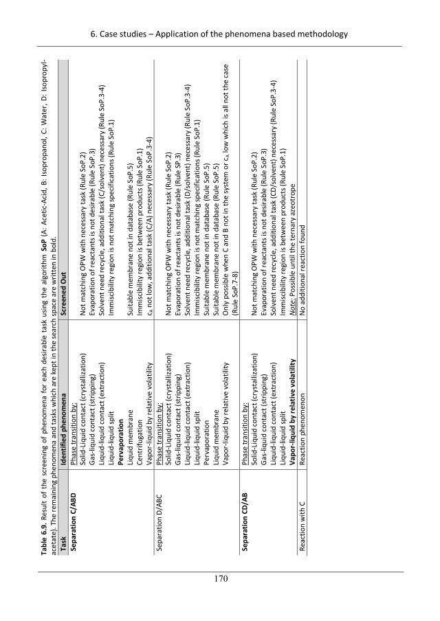
6. Case studies – Application of the phenomena based methodology
170
Tabl
e 6.
9. R
esul
t of
the
scr
eeni
ng o
f ph
enom
ena
for
each
des
irabl
e ta
sk u
sing
the
algo
rithm
SoP
(A:
Ace
tic-A
cid,
B: I
sopr
opan
ol, C
: Wat
er, D
: Iso
prop
yl-
acet
ate)
. The
rem
aini
ng p
heno
men
a an
d ta
sks w
hich
are
kep
t in
the
sear
ch sp
ace
are
writ
ten
in b
old.
Ta
sk
Iden
tifie
d ph
enom
ena
Scre
ened
Out
Se
para
tion
C/AB
D Ph
ase
tran
sitio
n by
: So
lid-L
iqui
d co
ntac
t (cr
ysta
lliza
tion)
G
as-li
quid
con
tact
(str
ippi
ng)
Liqu
id-li
quid
con
tact
(ext
ract
ion)
Li
quid
-liqu
id sp
lit
Perv
apor
atio
n Li
quid
mem
bran
e Ce
ntrif
ugat
ion
Vapo
r-liq
uid
by re
lativ
e vo
latil
ity
Not
mat
chin
g O
PW w
ith n
eces
sary
task
(Rul
e So
P.2)
Ev
apor
atio
n of
reac
tant
s is n
ot d
esira
ble
(Rul
e So
P.3)
So
lven
t nee
d re
cycl
e, a
dditi
onal
task
(C/s
olve
nt) n
eces
sary
(Rul
e So
P.3-
4)
Imm
iscib
ility
regi
on is
not
mat
chin
g sp
ecifi
catio
ns (R
ule
SoP.
1)
Suita
ble
mem
bran
e no
t in
data
base
(Rul
e So
P.5)
Im
misc
ibili
ty re
gion
is b
etw
een
prod
ucts
(Rul
e So
P.1)
c A
not
low
, add
ition
al ta
sk (C
/A) n
eces
sary
(Rul
e So
P.3-
4)
Sepa
ratio
n D/
ABC
Phas
e tr
ansit
ion
by:
Solid
-Liq
uid
cont
act (
crys
talli
zatio
n)
Gas
-liqu
id c
onta
ct (s
trip
ping
) Li
quid
-liqu
id c
onta
ct (e
xtra
ctio
n)
Liqu
id-li
quid
split
Pe
rvap
orat
ion
Liqu
id m
embr
ane
Vapo
r-liq
uid
by re
lativ
e vo
latil
ity
Not
mat
chin
g O
PW w
ith n
eces
sary
task
(Rul
e So
P.2)
Ev
apor
atio
n of
reac
tant
s is n
ot d
esira
ble
(Rul
e SP
.3)
Solv
ent n
eed
recy
cle,
add
ition
al ta
sk (D
/sol
vent
) nec
essa
ry (R
ule
SoP.
3-4)
Im
misc
ibili
ty re
gion
is n
ot m
atch
ing
spec
ifica
tions
(Rul
e So
P.1)
Su
itabl
e m
embr
ane
not i
n da
taba
se (R
ule
SoP.
5)
Suita
ble
mem
bran
e no
t in
data
base
(Rul
e So
P.5)
O
nly
poss
ible
whe
n C
and
B no
t in
the
syst
em o
r cA l
ow w
hich
is a
ll no
t the
cas
e (R
ule
SoP.
7-8)
Se
para
tion
CD/A
B Ph
ase
tran
sitio
n by
: So
lid-L
iqui
d co
ntac
t (cr
ysta
lliza
tion)
G
as-li
quid
con
tact
(str
ippi
ng)
Liqu
id-li
quid
con
tact
(ext
ract
ion)
Li
quid
-liqu
id sp
lit
Vapo
r-liq
uid
by re
lativ
e vo
latil
ity
Not
mat
chin
g O
PW w
ith n
eces
sary
task
(Rul
e So
P.2)
Ev
apor
atio
n of
reac
tant
s is n
ot d
esira
ble
(Rul
e So
P.3)
So
lven
t nee
d re
cycl
e, a
dditi
onal
task
(CD/
solv
ent)
nece
ssar
y (R
ule
SoP.
3-4)
Im
misc
ibili
ty re
gion
is b
etw
een
prod
ucts
(Rul
e So
P.1)
No
te: P
ossib
le u
ntil
the
tern
ary
azeo
trop
e Re
actio
n w
ith C
Re
actio
n ph
enom
enon
N
o ad
ditio
nal r
eact
ion
foun
d
200
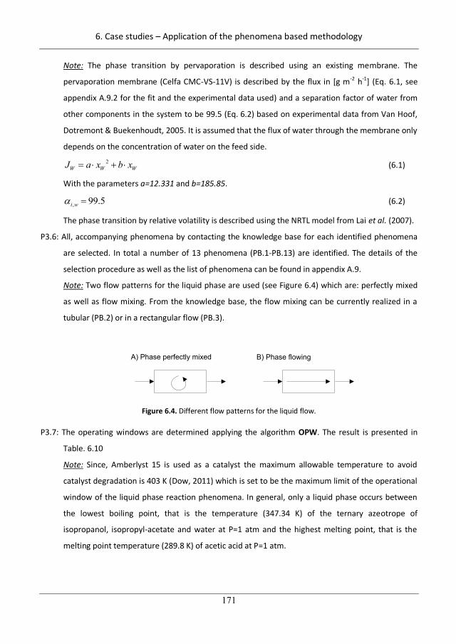
6. Case studies – Application of the phenomena based methodology
171
Note: The phase transition by pervaporation is described using an existing membrane. The
pervaporation membrane (Celfa CMC-VS-11V) is described by the flux in [g m-2 h-1] (Eq. 6.1, see
appendix A.9.2 for the fit and the experimental data used) and a separation factor of water from
other components in the system to be 99.5 (Eq. 6.2) based on experimental data from Van Hoof,
Dotremont & Buekenhoudt, 2005. It is assumed that the flux of water through the membrane only
depends on the concentration of water on the feed side.
2W W WJ a x b x (6.1)
With the parameters a=12.331 and b=185.85.
, 99.5i w (6.2)
The phase transition by relative volatility is described using the NRTL model from Lai et al. (2007).
P3.6: All, accompanying phenomena by contacting the knowledge base for each identified phenomena
are selected. In total a number of 13 phenomena (PB.1-PB.13) are identified. The details of the
selection procedure as well as the list of phenomena can be found in appendix A.9.
Note: Two flow patterns for the liquid phase are used (see Figure 6.4) which are: perfectly mixed
as well as flow mixing. From the knowledge base, the flow mixing can be currently realized in a
tubular (PB.2) or in a rectangular flow (PB.3).
A) Phase perfectly mixed B) Phase flowing
Figure 6.4. Different flow patterns for the liquid flow.
P3.7: The operating windows are determined applying the algorithm OPW. The result is presented in
Table. 6.10
Note: Since, Amberlyst 15 is used as a catalyst the maximum allowable temperature to avoid
catalyst degradation is 403 K (Dow, 2011) which is set to be the maximum limit of the operational
window of the liquid phase reaction phenomena. In general, only a liquid phase occurs between
the lowest boiling point, that is the temperature (347.34 K) of the ternary azeotrope of
isopropanol, isopropyl-acetate and water at P=1 atm and the highest melting point, that is the
melting point temperature (289.8 K) of acetic acid at P=1 atm.
201
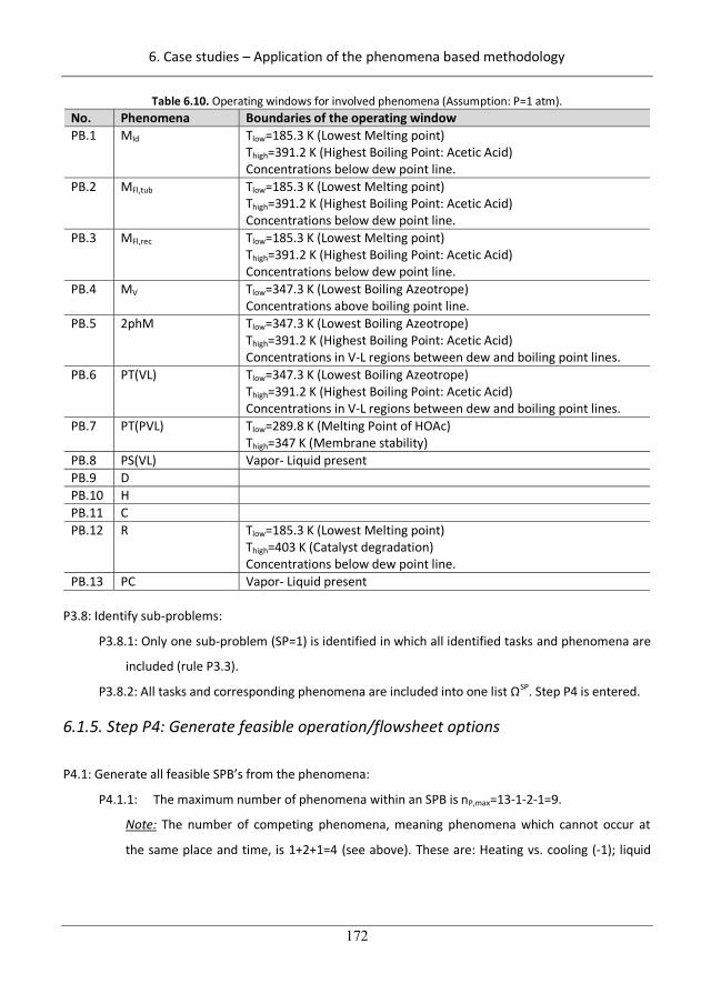
6. Case studies – Application of the phenomena based methodology
172
Table 6.10. Operating windows for involved phenomena (Assumption: P=1 atm). No. Phenomena Boundaries of the operating window PB.1 MId Tlow=185.3 K (Lowest Melting point)
Thigh=391.2 K (Highest Boiling Point: Acetic Acid) Concentrations below dew point line.
PB.2 MFl,tub Tlow=185.3 K (Lowest Melting point) Thigh=391.2 K (Highest Boiling Point: Acetic Acid) Concentrations below dew point line.
PB.3 MFl,rec Tlow=185.3 K (Lowest Melting point) Thigh=391.2 K (Highest Boiling Point: Acetic Acid) Concentrations below dew point line.
PB.4 MV Tlow=347.3 K (Lowest Boiling Azeotrope) Concentrations above boiling point line.
PB.5 2phM Tlow=347.3 K (Lowest Boiling Azeotrope) Thigh=391.2 K (Highest Boiling Point: Acetic Acid) Concentrations in V-L regions between dew and boiling point lines.
PB.6 PT(VL) Tlow=347.3 K (Lowest Boiling Azeotrope) Thigh=391.2 K (Highest Boiling Point: Acetic Acid) Concentrations in V-L regions between dew and boiling point lines.
PB.7 PT(PVL) Tlow=289.8 K (Melting Point of HOAc) Thigh=347 K (Membrane stability)
PB.8 PS(VL) Vapor- Liquid present PB.9 D PB.10 H PB.11 C PB.12 R Tlow=185.3 K (Lowest Melting point)
Thigh=403 K (Catalyst degradation) Concentrations below dew point line.
PB.13 PC Vapor- Liquid present P3.8: Identify sub-problems:
P3.8.1: Only one sub-problem (SP=1) is identified in which all identified tasks and phenomena are
included (rule P3.3).
P3.8.2: All tasks and corresponding phenomena are included into one list SP. Step P4 is entered.
6.1.5. Step P4: Generate feasible operation/flowsheet options
P4.1: Generate all feasible SPB’s from the phenomena:
P4.1.1: The maximum number of phenomena within an SPB is nP,max=13-1-2-1=9.
Note: The number of competing phenomena, meaning phenomena which cannot occur at
the same place and time, is 1+2+1=4 (see above). These are: Heating vs. cooling (-1); liquid
202
6. Case studies – Application of the phenomena based methodology
173
mixing patterns flow and perfectly mixed cannot be connected within one SPB (-2); the
dividing phenomenon is by definition a single phenomenon SPB itself (-1).
P4.1.2: Interconnect all phenomena in the search space to SPB’s by using the connectivity rules
for each phenomenon (see table 2.6):
The number of phenomena is nP,tot,=13. Therefore, in total a number of 4019 SPB’s is
generated (Eq.6.3).
,max,
max1 ,
1 !1 4019
1 ! !
PnP tot
k P tot
nNSPB
n k k
(6.3)
P4.1.3: Screening of all SPB’s for feasibility: Using connectivity rules and the information of the
operating window of each phenomenon, a total number of 58 SPB’s are feasible in terms of
conditions of the operatings windows of the integrated phenomena. All 58 feasible SPB’s are
shown in Table 6.11.
Note: M=R=C=2phM only allows vapor-liquid inlet since heat of reaction is not enough for
vaporization. Additional cooling would lead to a decrease in temperature and therefore
would enable condensation of the vapor and not vaporization of the liquid.
203
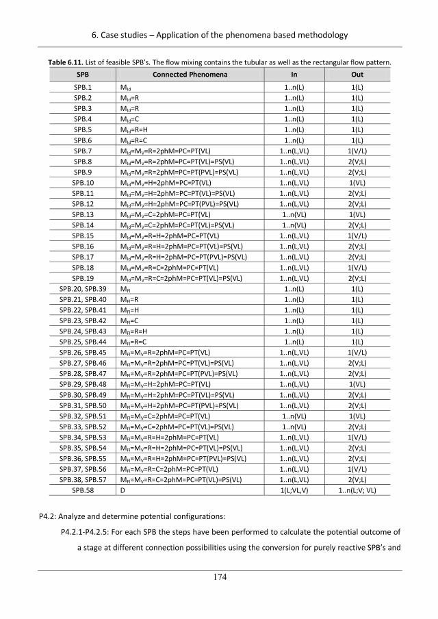
6. Case studies – Application of the phenomena based methodology
174
Table 6.11. List of feasible SPB’s. The flow mixing contains the tubular as well as the rectangular flow pattern. SPB Connected Phenomena In Out
SPB.1 MId 1..n(L) 1(L) SPB.2 MId=R 1..n(L) 1(L) SPB.3 MId=R 1..n(L) 1(L) SPB.4 MId=C 1..n(L) 1(L) SPB.5 MId=R=H 1..n(L) 1(L) SPB.6 MId=R=C 1..n(L) 1(L) SPB.7 MId=MV=R=2phM=PC=PT(VL) 1..n(L,VL) 1(V/L) SPB.8 MId=MV=R=2phM=PC=PT(VL)=PS(VL) 1..n(L,VL) 2(V;L) SPB.9 MId=MV=R=2phM=PC=PT(PVL)=PS(VL) 1..n(L,VL) 2(V;L)
SPB.10 MId=MV=H=2phM=PC=PT(VL) 1..n(L,VL) 1(VL) SPB.11 MId=MV=H=2phM=PC=PT(VL)=PS(VL) 1..n(L,VL) 2(V;L) SPB.12 MId=MV=H=2phM=PC=PT(PVL)=PS(VL) 1..n(L,VL) 2(V;L) SPB.13 MId=MV=C=2phM=PC=PT(VL) 1..n(VL) 1(VL) SPB.14 MId=MV=C=2phM=PC=PT(VL)=PS(VL) 1..n(VL) 2(V;L) SPB.15 MId=MV=R=H=2phM=PC=PT(VL) 1..n(L,VL) 1(V/L) SPB.16 MId=MV=R=H=2phM=PC=PT(VL)=PS(VL) 1..n(L,VL) 2(V;L) SPB.17 MId=MV=R=H=2phM=PC=PT(PVL)=PS(VL) 1..n(L,VL) 2(V;L) SPB.18 MId=MV=R=C=2phM=PC=PT(VL) 1..n(L,VL) 1(V/L) SPB.19 MId=MV=R=C=2phM=PC=PT(VL)=PS(VL) 1..n(L,VL) 2(V;L)
SPB.20, SPB.39 MFl 1..n(L) 1(L) SPB.21, SPB.40 MFl=R 1..n(L) 1(L) SPB.22, SPB.41 MFl=H 1..n(L) 1(L) SPB.23, SPB.42 MFl=C 1..n(L) 1(L) SPB.24, SPB.43 MFl=R=H 1..n(L) 1(L) SPB.25, SPB.44 MFl=R=C 1..n(L) 1(L) SPB.26, SPB.45 MFl=MV=R=2phM=PC=PT(VL) 1..n(L,VL) 1(V/L) SPB.27, SPB.46 MFl=MV=R=2phM=PC=PT(VL)=PS(VL) 1..n(L,VL) 2(V;L) SPB.28, SPB.47 MFl=MV=R=2phM=PC=PT(PVL)=PS(VL) 1..n(L,VL) 2(V;L) SPB.29, SPB.48 MFl=MV=H=2phM=PC=PT(VL) 1..n(L,VL) 1(VL) SPB.30, SPB.49 MFl=MV=H=2phM=PC=PT(VL)=PS(VL) 1..n(L,VL) 2(V;L) SPB.31, SPB.50 MFl=MV=H=2phM=PC=PT(PVL)=PS(VL) 1..n(L,VL) 2(V;L) SPB.32, SPB.51 MFl=MV=C=2phM=PC=PT(VL) 1..n(VL) 1(VL) SPB.33, SPB.52 MFl=MV=C=2phM=PC=PT(VL)=PS(VL) 1..n(VL) 2(V;L) SPB.34, SPB.53 MFl=MV=R=H=2phM=PC=PT(VL) 1..n(L,VL) 1(V/L) SPB.35, SPB.54 MFl=MV=R=H=2phM=PC=PT(VL)=PS(VL) 1..n(L,VL) 2(V;L) SPB.36, SPB.55 MFl=MV=R=H=2phM=PC=PT(PVL)=PS(VL) 1..n(L,VL) 2(V;L) SPB.37, SPB.56 MFl=MV=R=C=2phM=PC=PT(VL) 1..n(L,VL) 1(V/L) SPB.38, SPB.57 MFl=MV=R=C=2phM=PC=PT(VL)=PS(VL) 1..n(L,VL) 2(V;L)
SPB.58 D 1(L;VL,V) 1..n(L;V; VL)
P4.2: Analyze and determine potential configurations:
P4.2.1-P4.2.5: For each SPB the steps have been performed to calculate the potential outcome of
a stage at different connection possibilities using the conversion for purely reactive SPB’s and
204
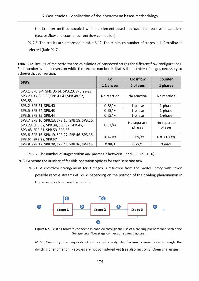
6. Case studies – Application of the phenomena based methodology
175
the Kremser method coupled with the element-based approach for reactive separations
(co,crossflow and counter current flow connection).
P4.2.6: The results are presented in table 6.12. The minimum number of stages is 1. Crossflow is
selected (Rule P4.7).
Table 6.12. Results of the performance calculation of connected stages for different flow configurations. First number is the conversion while the second number indicates the number of stages necessary to achieve that conversion.
SPB’s Co Crossflow Counter
1,2 phases 2 phases 2 phases SPB.1, SPB.3-4, SPB.10-14, SPB.20, SPB.22-23, SPB.29-33, SPB.39,SPB.41-42,SPB.48-52, SPB.58
No reaction No reaction No reaction
SPB.2, SPB.21, SPB.40 0.58/ 1-phase 1-phase SPB.5, SPB.24, SPB.43 0.55/ 1-phase 1-phase SPB.6, SPB.25, SPB.44 0.65/ 1-phase 1-phase SPB.7, SPB.10, SPB.13, SPB.15, SPB.18, SPB.26, SPB.29, SPB.32, SPB.34, SPB.37, SPB.45, SPB.48, SPB.51, SPB.53, SPB.56
0.57/ No separate phases
No separate phases
SPB.8, SPB.16, SPB.19, SPB.27, SPB.46, SPB.35, SPB.54, SPB.38, SPB.57 0. 67/ 0. 69/ 0.81/13( )
SPB.9, SPB.17, SPB.28, SPB.47, SPB.36, SPB.55 0.99/1 0.99/1 0.99/1
P4.2.7: The number of stages within one process is between 1 and 3 (Rule P4.10).
P4.3: Generate the number of feasible operation options for each separate task:
P4.3.1: A crossflow arrangement for 3 stages is retrieved from the model library with seven
possible recycle streams of liquid depending on the position of the dividing phenomenon in
the superstructure (see Figure 6.5).
Figure 6.5. Existing forward connections enabled through the use of a dividing phenomenon within the
3-stage crossflow stage connection superstructure.
Note: Currently, the superstructure contains only the forward connections through the
dividing phenomenon. Recycles are not considered yet (see also section 8: Open challenges).
205
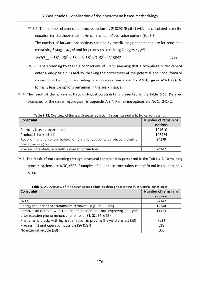
6. Case studies – Application of the phenomena based methodology
176
P4.3.2: The number of generated process options is 218892 (Eq.6.4) which is calculated from the
equation for the theoretical maximum number of operation options (Eq. 3.3).
The number of forward connections enabled by the dividing phenomenon are for processes
containing 3 stages nR,3=6 and for processes containing 2 stages nR,2=3. 3 2 1 2 1
max 58 58 58 6 58 3 58 218892NOO (6.4)
P4.3.3: The screening by feasible connections of SPB’s, meaning that a two-phase outlet cannot
enter a one-phase SPB and by checking the correctness of the potential additional forward
connections through the dividing phenomenon (see appendix A.9.4), gives NOO=121610
formally feasible options remaining in the search space.
P4.4: The result of the screening through logical constraints is presented in the table 6.13. Detailed
examples for the screening are given in appendix A.9.4. Remaining options are NOOL=24142.
Table 6.13. Overview of the search space reduction through screening by logical constraints. Constraint Number of remaining
options Formally feasible operations: 121610 Product is formed (L1) 102424 Reaction phenomenon before or simultaneously with phase transition phenomenon (L2)
64179
Process potentially acts within operating window 24142 P4.5: The result of the screening through structural constraints is presented in the Table 6.2. Remaining
process options are NOOS=506. Examples of all applied constraints can be found in the appendix
A.9.6.
Table 6.14. Overview of the search space reduction through screening by structural constraints. Constraint Number of remaining
options NPOL 24142 Energy redundant operations are removed ; e.g. –H–C– (S5) 12244 Remove all options with redundant phenomena not improving the yield after reaction phenomenon/phenomena (S1, S2, S4 & S9)
11153
Phenomena blocks with highest effect on improving the yield are last (S3) 7619 Process in 1 unit operation possible (S6 & S7) 518 No external recycle (S8) 506
206
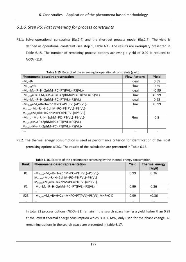
6. Case studies – Application of the phenomena based methodology
177
6.1.6. Step P5: Fast screening for process constraints
P5.1: Solve operational constraints (Eq.2.4) and the short-cut process model (Eq.2.7). The yield is
defined as operational constraint (see step 1, Table 6.1). The results are exemplary presented in
Table 6.15. The number of remaining process options achieving a yield of 0.99 is reduced to
NOOO=118.
Table 6.15. Excerpt of the screening by operational constraints (yield). Phenomena-based representation Flow-Pattern Yield -MId=R- Ideal 0.65 -MFl,tub=R- Flow 0.65 -MId=MV=R=H=2phM=PC=PT(PVL)=PS(VL)- Ideal >0.99 -MFl,tub=R=H-MFl=MV=R=H=2phM=PC=PT(PVL)=PS(VL)- Flow >0.99 -MId=MV=R=H=2phM=PC=PT(VL)=PS(VL) Ideal 0.68 -MF,tubl=MV=R=H=2phM=PC=PT(PVL)=PS(VL)- MFl,tub=MV=R=H=2phM=PC=PT(PVL)=PS(VL)- MFl,tub=MV=R=H=2phM=PC=PT(PVL)=PS(VL)-
Flow >0.99
-MFl,rec=MV=R=H=2phM=PC=PT(VL)=PS(VL)- MFl,rec=MV=R=2phM=PC=PT(PVL)=PS(VL)- MFl,rec=MV=R=2phM=PC=PT(PVL)=PS(VL)-
Flow 0.8
…. … … P5.2: The thermal energy consumption is used as performance criterion for identification of the most
promising options NOOP: The results of the calculation are presented in Table 6.16.
Table 6.16. Excerpt of the performance screening by the thermal energy consumption. Rank Phenomena-based representation Yield Thermal energy
[MW] #1 -MFl,tub=MV=R=H=2phM=PC=PT(PVL)=PS(VL)-
MFl,tub=MV=R=H=2phM=PC=PT(PVL)=PS(VL)- MFl,tub=MV=R=H=2phM=PC=PT(PVL)=PS(VL)-
0.99 0.36
#1 -MId=MV=R=H=2phM=PC=PT(PVL)=PS(VL)- 0.99 0.36 … … … …
#23 -MId,tub=MV=R=H=2phM=PC=PT(PVL)=PS(VL)-M=R=C-D 0.99 >0.36 … … … …
In total 22 process options (NOOP=22) remain in the search space having a yield higher than 0.99
at the lowest thermal energy consumption which is 0.36 MW, only used for the phase change. All
remaining options in the search space are presented in table 6.17.
207
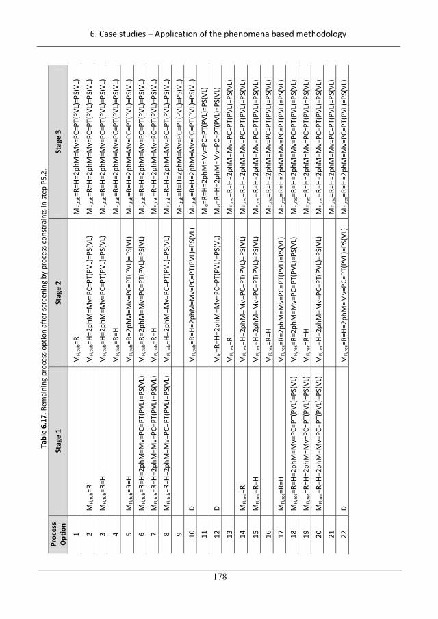
6. Case studies – Application of the phenomena based methodology
178
Tabl
e 6.
17. R
emai
ning
pro
cess
opt
ion
afte
r scr
eeni
ng b
y pr
oces
s con
stra
ints
in st
ep P
5.2.
Pr
oces
s O
ptio
n St
age
1 St
age
2 St
age
3
1
MFl
,tub=
R M
Fl,tu
b=R=
H=2p
hM=M
v=PC
=PT(
PVL)
=PS(
VL)
2 M
Fl,tu
b=R
MFl
,tub=
H=2p
hM=M
v=PC
=PT(
PVL)
=PS(
VL)
MFl
,tub=
R=H=
2phM
=Mv=
PC=P
T(PV
L)=P
S(VL
)
3 M
Fl,tu
b=R=
H M
Fl,tu
b=H=
2phM
=Mv=
PC=P
T(PV
L)=P
S(VL
) M
Fl,tu
b=R=
H=2p
hM=M
v=PC
=PT(
PVL)
=PS(
VL)
4
MFl
,tub=
R=H
MFl
,tub=
R=H=
2phM
=Mv=
PC=P
T(PV
L)=P
S(VL
)
5 M
Fl,tu
b=R=
H M
Fl,tu
b=R=
2phM
=Mv=
PC=P
T(PV
L)=P
S(VL
) M
Fl,tu
b=R=
H=2p
hM=M
v=PC
=PT(
PVL)
=PS(
VL)
6 M
Fl,tu
b=R=
H=2p
hM=M
v=PC
=PT(
PVL)
=PS(
VL)
MFl
,tub=
R=2p
hM=M
v=PC
=PT(
PVL)
=PS(
VL)
MFl
,tub=
R=H=
2phM
=Mv=
PC=P
T(PV
L)=P
S(VL
)
7 M
Fl,tu
b=R=
H=2p
hM=M
v=PC
=PT(
PVL)
=PS(
VL)
MFl
,tub=
R=H
MFl
,tub=
R=H=
2phM
=Mv=
PC=P
T(PV
L)=P
S(VL
)
8 M
Fl,tu
b=R=
H=2p
hM=M
v=PC
=PT(
PVL)
=PS(
VL)
MFl
,tub=
H=2p
hM=M
v=PC
=PT(
PVL)
=PS(
VL)
MFl
,tub=
R=H=
2phM
=Mv=
PC=P
T(PV
L)=P
S(VL
)
9
M
Fl,tu
b=R=
H=2p
hM=M
v=PC
=PT(
PVL)
=PS(
VL)
10
D M
Fl,tu
b=R=
H=2p
hM=M
v=PC
=PT(
PVL)
=PS(
VL)
MFl
,tub=
R=H=
2phM
=Mv=
PC=P
T(PV
L)=P
S(VL
)
11
Mid
=R=H
=2ph
M=M
v=PC
=PT(
PVL)
=PS(
VL)
12
D M
id=R
=H=2
phM
=Mv=
PC=P
T(PV
L)=P
S(VL
) M
id=R
=H=2
phM
=Mv=
PC=P
T(PV
L)=P
S(VL
)
13
M
Fl,re
c=R
MFl
,rec=
R=H=
2phM
=Mv=
PC=P
T(PV
L)=P
S(VL
)
14
MFl
,rec=
R M
Fl,re
c=H=
2phM
=Mv=
PC=P
T(PV
L)=P
S(VL
) M
Fl,re
c=R=
H=2p
hM=M
v=PC
=PT(
PVL)
=PS(
VL)
15
MFl
,rec=
R=H
MFl
,rec=
H=2p
hM=M
v=PC
=PT(
PVL)
=PS(
VL)
MFl
,rec=
R=H=
2phM
=Mv=
PC=P
T(PV
L)=P
S(VL
)
16
M
Fl,re
c=R=
H M
Fl,re
c=R=
H=2p
hM=M
v=PC
=PT(
PVL)
=PS(
VL)
17
MFl
,rec=
R=H
MFl
,rec=
R=2p
hM=M
v=PC
=PT(
PVL)
=PS(
VL)
MFl
,rec=
R=H=
2phM
=Mv=
PC=P
T(PV
L)=P
S(VL
)
18
MFl
,rec=
R=H=
2phM
=Mv=
PC=P
T(PV
L)=P
S(VL
) M
Fl,re
c=R=
2phM
=Mv=
PC=P
T(PV
L)=P
S(VL
) M
Fl,re
c=R=
H=2p
hM=M
v=PC
=PT(
PVL)
=PS(
VL)
19
MFl
,rec=
R=H=
2phM
=Mv=
PC=P
T(PV
L)=P
S(VL
) M
Fl,re
c=R=
H M
Fl,re
c=R=
H=2p
hM=M
v=PC
=PT(
PVL)
=PS(
VL)
20
MFl
,rec=
R=H=
2phM
=Mv=
PC=P
T(PV
L)=P
S(VL
) M
Fl,re
c=H=
2phM
=Mv=
PC=P
T(PV
L)=P
S(VL
) M
Fl,re
c=R=
H=2p
hM=M
v=PC
=PT(
PVL)
=PS(
VL)
21
MFl
,rec=
R=H=
2phM
=Mv=
PC=P
T(PV
L)=P
S(VL
)
22
D M
Fl,re
c=R=
H=2p
hM=M
v=PC
=PT(
PVL)
=PS(
VL)
MFl
,rec=
R=H=
2phM
=Mv=
PC=P
T(PV
L)=P
S(VL
)
208
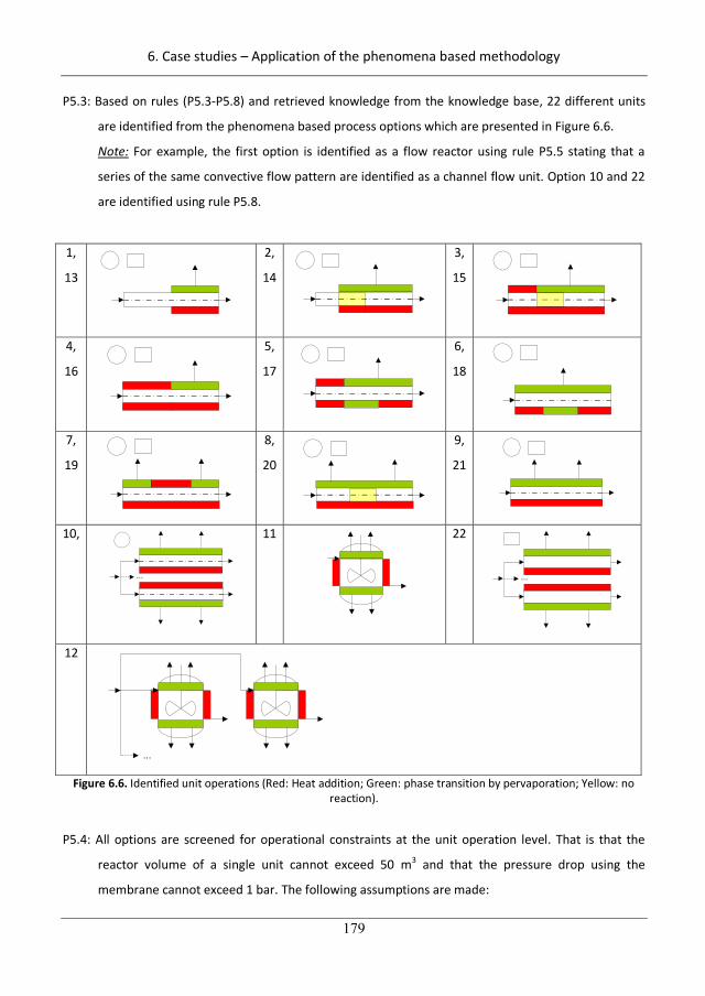
6. Case studies – Application of the phenomena based methodology
179
P5.3: Based on rules (P5.3-P5.8) and retrieved knowledge from the knowledge base, 22 different units
are identified from the phenomena based process options which are presented in Figure 6.6.
Note: For example, the first option is identified as a flow reactor using rule P5.5 stating that a
series of the same convective flow pattern are identified as a channel flow unit. Option 10 and 22
are identified using rule P5.8.
1,
13
2,
14
3,
15
4,
16
5,
17
6,
18
7,
19
8,
20
9,
21
10,
...
11
22
...
12
... Figure 6.6. Identified unit operations (Red: Heat addition; Green: phase transition by pervaporation; Yellow: no
reaction).
P5.4: All options are screened for operational constraints at the unit operation level. That is that the
reactor volume of a single unit cannot exceed 50 m3 and that the pressure drop using the
membrane cannot exceed 1 bar. The following assumptions are made:
209
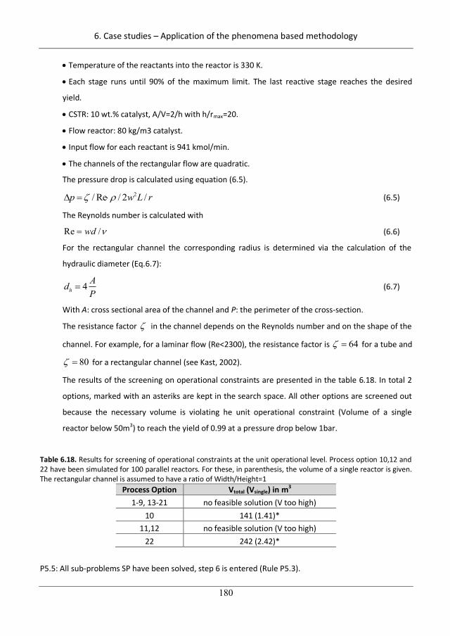
6. Case studies – Application of the phenomena based methodology
180
Temperature of the reactants into the reactor is 330 K.
Each stage runs until 90% of the maximum limit. The last reactive stage reaches the desired
yield.
CSTR: 10 wt.% catalyst, A/V=2/h with h/rmax=20.
Flow reactor: 80 kg/m3 catalyst.
Input flow for each reactant is 941 kmol/min.
The channels of the rectangular flow are quadratic.
The pressure drop is calculated using equation (6.5). 2/ Re / 2 /p w L r (6.5)
The Reynolds number is calculated with
Re /wd (6.6)
For the rectangular channel the corresponding radius is determined via the calculation of the
hydraulic diameter (Eq.6.7):
4hAdP
(6.7)
With A: cross sectional area of the channel and P: the perimeter of the cross-section.
The resistance factor in the channel depends on the Reynolds number and on the shape of the
channel. For example, for a laminar flow (Re<2300), the resistance factor is 64 for a tube and
80 for a rectangular channel (see Kast, 2002).
The results of the screening on operational constraints are presented in the table 6.18. In total 2
options, marked with an asteriks are kept in the search space. All other options are screened out
because the necessary volume is violating he unit operational constraint (Volume of a single
reactor below 50m3) to reach the yield of 0.99 at a pressure drop below 1bar.
Table 6.18. Results for screening of operational constraints at the unit operational level. Process option 10,12 and 22 have been simulated for 100 parallel reactors. For these, in parenthesis, the volume of a single reactor is given. The rectangular channel is assumed to have a ratio of Width/Height=1
Process Option Vtotal (Vsingle) in m3 1-9, 13-21 no feasible solution (V too high)
10 141 (1.41)* 11,12 no feasible solution (V too high)
22 242 (2.42)*
P5.5: All sub-problems SP have been solved, step 6 is entered (Rule P5.3).
210
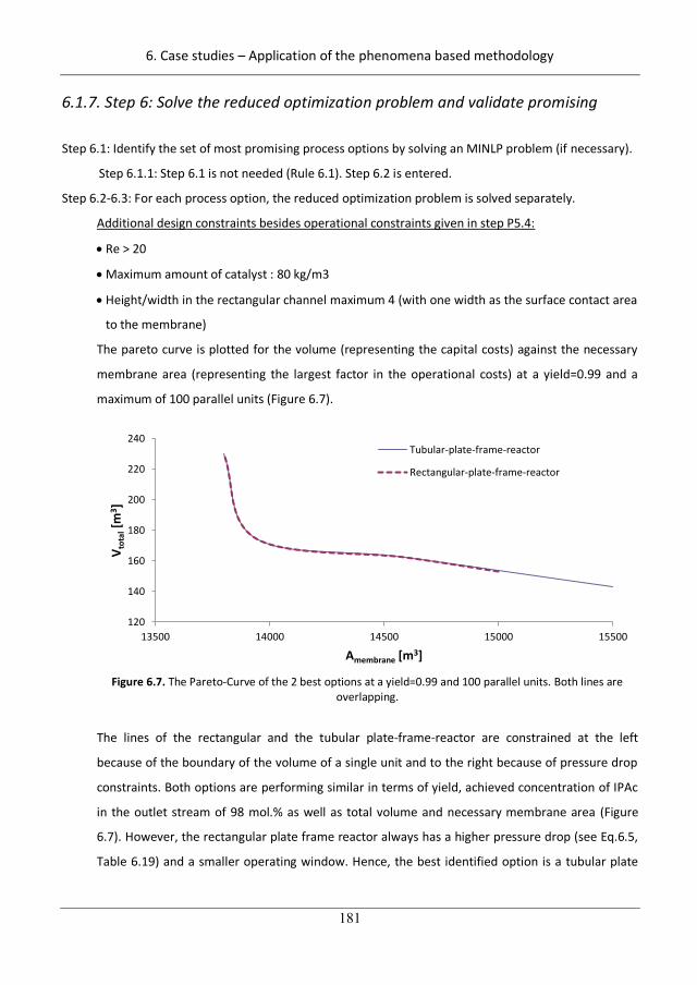
6. Case studies – Application of the phenomena based methodology
181
6.1.7. Step 6: Solve the reduced optimization problem and validate promising
Step 6.1: Identify the set of most promising process options by solving an MINLP problem (if necessary).
Step 6.1.1: Step 6.1 is not needed (Rule 6.1). Step 6.2 is entered.
Step 6.2-6.3: For each process option, the reduced optimization problem is solved separately.
Additional design constraints besides operational constraints given in step P5.4:
Re > 20
Maximum amount of catalyst : 80 kg/m3
Height/width in the rectangular channel maximum 4 (with one width as the surface contact area
to the membrane)
The pareto curve is plotted for the volume (representing the capital costs) against the necessary
membrane area (representing the largest factor in the operational costs) at a yield=0.99 and a
maximum of 100 parallel units (Figure 6.7).
120
140
160
180
200
220
240
13500 14000 14500 15000 15500
V tot
al[m
3 ]
Amembrane [m3]
Tubular-plate-frame-reactor
Rectangular-plate-frame-reactor
Figure 6.7. The Pareto-Curve of the 2 best options at a yield=0.99 and 100 parallel units. Both lines are
overlapping.
The lines of the rectangular and the tubular plate-frame-reactor are constrained at the left
because of the boundary of the volume of a single unit and to the right because of pressure drop
constraints. Both options are performing similar in terms of yield, achieved concentration of IPAc
in the outlet stream of 98 mol.% as well as total volume and necessary membrane area (Figure
6.7). However, the rectangular plate frame reactor always has a higher pressure drop (see Eq.6.5,
Table 6.19) and a smaller operating window. Hence, the best identified option is a tubular plate
211
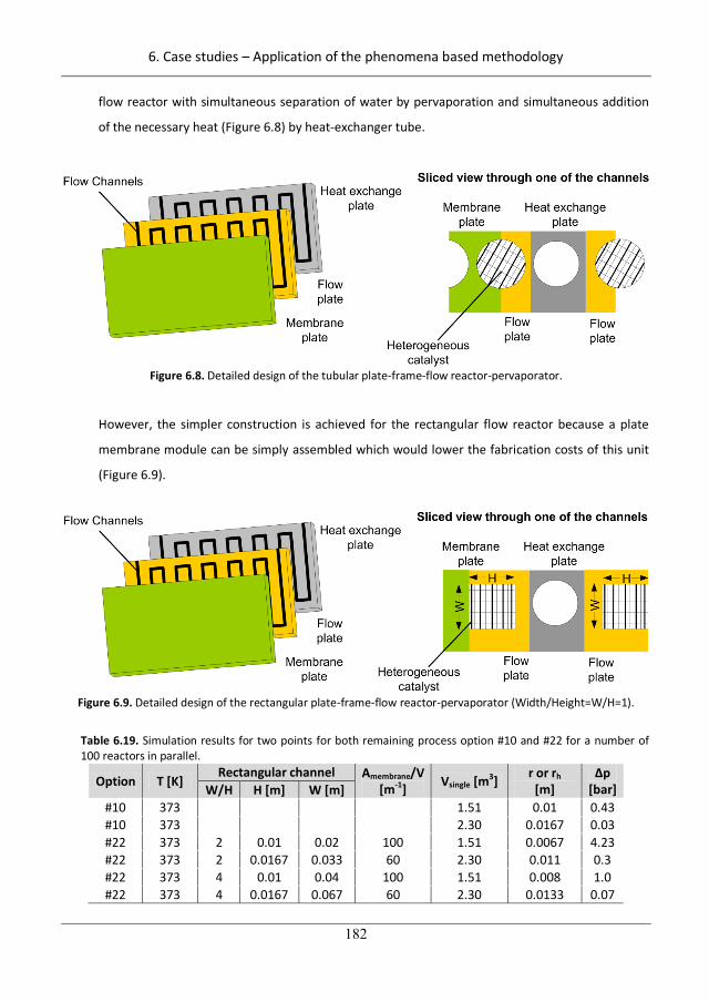
6. Case studies – Application of the phenomena based methodology
182
flow reactor with simultaneous separation of water by pervaporation and simultaneous addition
of the necessary heat (Figure 6.8) by heat-exchanger tube.
Figure 6.8. Detailed design of the tubular plate-frame-flow reactor-pervaporator.
However, the simpler construction is achieved for the rectangular flow reactor because a plate
membrane module can be simply assembled which would lower the fabrication costs of this unit
(Figure 6.9).
Figure 6.9. Detailed design of the rectangular plate-frame-flow reactor-pervaporator (Width/Height=W/H=1).
Table 6.19. Simulation results for two points for both remaining process option #10 and #22 for a number of 100 reactors in parallel.
Option T [K] Rectangular channel Amembrane/V
[m-1] Vsingle [m3] r or rh [m]
p [bar] W/H H [m] W [m]
#10 373 1.51 0.01 0.43 #10 373 2.30 0.0167 0.03 #22 373 2 0.01 0.02 100 1.51 0.0067 4.23 #22 373 2 0.0167 0.033 60 2.30 0.011 0.3 #22 373 4 0.01 0.04 100 1.51 0.008 1.0 #22 373 4 0.0167 0.067 60 2.30 0.0133 0.07
212
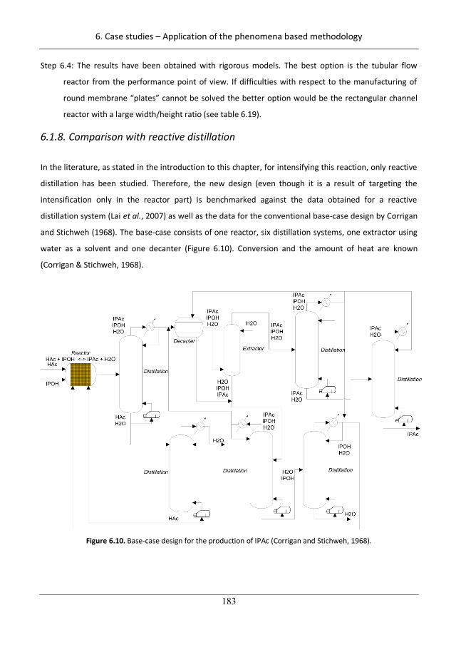
6. Case studies – Application of the phenomena based methodology
183
Step 6.4: The results have been obtained with rigorous models. The best option is the tubular flow
reactor from the performance point of view. If difficulties with respect to the manufacturing of
round membrane “plates” cannot be solved the better option would be the rectangular channel
reactor with a large width/height ratio (see table 6.19).
6.1.8. Comparison with reactive distillation
In the literature, as stated in the introduction to this chapter, for intensifying this reaction, only reactive
distillation has been studied. Therefore, the new design (even though it is a result of targeting the
intensification only in the reactor part) is benchmarked against the data obtained for a reactive
distillation system (Lai et al., 2007) as well as the data for the conventional base-case design by Corrigan
and Stichweh (1968). The base-case consists of one reactor, six distillation systems, one extractor using
water as a solvent and one decanter (Figure 6.10). Conversion and the amount of heat are known
(Corrigan & Stichweh, 1968).
Figure 6.10. Base-case design for the production of IPAc (Corrigan and Stichweh, 1968).
213
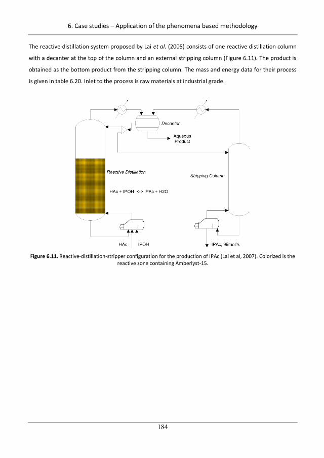
6. Case studies – Application of the phenomena based methodology
184
The reactive distillation system proposed by Lai et al. (2005) consists of one reactive distillation column
with a decanter at the top of the column and an external stripping column (Figure 6.11). The product is
obtained as the bottom product from the stripping column. The mass and energy data for their process
is given in table 6.20. Inlet to the process is raw materials at industrial grade.
Figure 6.11. Reactive-distillation-stripper configuration for the production of IPAc (Lai et al, 2007). Colorized is the
reactive zone containing Amberlyst-15.
214
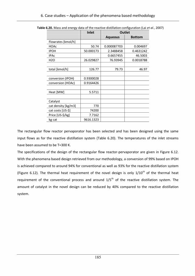
6. Case studies – Application of the phenomena based methodology
185
Table 6.20. Mass and energy data of the reactive distillation configuration (Lai et al., 2007) Inlet Outlet Aqueous Bottom
Flowrates [kmol/h] HOAc 50.74 0.000087703 0.004697 IPOH 50.000173 2.3488458 0.4631242 IPAc 0.6657455 46.5003 H2O 26.029827 76.93945 0.0018788 total [kmol/h] 126.77 79.73 46.97 conversion (IPOH) 0.9300028 conversion (HOAc) 0.9164426 Heat [MW] 5.5711 Catalyst cat density [kg/m3] 770 cat costs [US-$] 74200 Price [US-$/kg] 7.7162 kg cat 9616.1323
The rectangular flow reactor pervaporator has been selected and has been designed using the same
input flows as for the reactive distillation system (Table 6.20). The temperatures of the inlet streams
have been assumed to be T=300 K.
The specifications of the design of the rectangular flow reactor-pervaporator are given in Figure 6.12.
With the phenomena based design retrieved from our methodology, a conversion of 99% based on IPOH
is achieved compared to around 94% for conventional as well as 93% for the reactive distillation system
(Figure 6.12). The thermal heat requirement of the novel design is only 1/10th of the thermal heat
requirement of the conventional process and around 1/5th of the reactive distillation system. The
amount of catalyst in the novel design can be reduced by 40% compared to the reactive distillation
system.
215
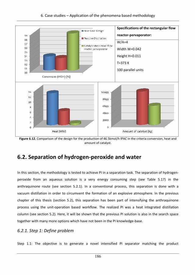
6. Case studies – Application of the phenomena based methodology
186
Specifications of the rectangular flow
reactor-pervaporator:
W/A=4
Width W=0.042
Height H=0.011
T=373 K
100 parallel units
Figure 6.12. Comparison of the design for the production of 46.5kmol/h IPAC in the criteria conversion, heat and amount of catalyst.
6.2. Separation of hydrogen-peroxide and water
In this section, the methodology is tested to achieve PI in a separation task. The separation of hydrogen-
peroxide from an aqueous solution is a very energy consuming step (see Table 5.17) in the
anthraquinone route (see section 5.2.1). In a conventional process, this separation is done with a
vacuum distillation in order to circumvent the formation of an explosive atmosphere. In the previous
chapter of this thesis (section 5.2), this separation has been part of intensifying the anthraquinone
process using the unit-operation based workflow. The realized PI was a heat integrated distillation
column (see section 5.2). Here, it will be shown that the previous PI solution is also in the search space
together with many more options which have not been in the PI knowledge-base.
6.2.1. Step 1: Define problem
Step 1.1: The objective is to generate a novel intensified PI separator matching the product
216
6. Case studies – Application of the phenomena based methodology
187
specifications in one unit and which minimizes the operational cost per kg product formed (Eq.6.8):
Obj RM,i , energy,i solvent,i 2 2min F = c + c c /RM i i i H O
RawMaterials Make UpEnergy
m E m m 2 2/ 2m/ii+ c+ c+ c+ c iii+ c+ c cc llc ,solvent,iRM,i ,RM,i ,RM i ,, solvent isolvent isolvent ienergy i lgy,gy,e e gy,energy,ienergy,ienergy ienergy ienergy ienergy ienergy ienergy i (6.8)
Step 1.2: The design scenario is the improvement of the separation process of H2O2 and water. The
process scenario is batch.
Step 1.3: A mixture stream (1000 kmol/h) containing 15 mol.% of H2O2 and 85mol.% water at T=308.15 K
and P=1 atm has to be purified to obtain a purity of H2O2 of 70 w.% of H2O2. The process is
continuous. The recovery of H2O2 in the purification should not be lower than 99 mol.%.
Step 1.4: Additional performance metric is selected which are simplification, energy, capital costs, (raw
material) efficiency as well as safety.
Step 1.5: The maturity is selected to a novel process.
Step 1.6.1-1.6.3: The performance metrics has been translated (Table 6.21).
All performance metric are translated into logical and structural constraints. The following
operational constraints are set:
Efficiency of product recovery (>99%),
Product purity >70 w.%
For screening with respect to performance metric (in step P5) is the costs of the purification of
H2O2.
Step 1.7: No base-case design exists. Therefore, step B2 is entered.
217
6. Case studies – Application of the phenomena based methodology
188
Table 6.21. Problem definition of the case study: separation of H2O2/ H2O. Fobj Operational costs (Eq. 6.8) Design scenario Design of PI equipment for the separation task Process scenario Continuous Logical constraints Only stream connection and operating window constraints
determined (in step A.2-P3). Structural constraints by PI metric Efficiency:
S1: Do not integrate units which inhibit each others performance. S2: Add phenomena and stages to the position in the flowsheet in which it has the highest efficiency. S3: Always end the flowsheet with the phenomena giving the highest yield last. Energy: S4: Do not connect units/stages with alternating heat addition and heat removal. S5: Do not connect units/stages with alternating pressures. S6: Integrate heat by connecting hot and cold streams whenever possible. Simplification: S7: Do not use repetitive (sequential) units. S8: Remove redundant stages not improving the yield/separation S9: Use only up to two different pressures in the system
Operational constraints (Rule 1.6) Purity of water (90 w.%) Purity of H2O2 (70 w.%) Boundaries of the explosive atmosphere (see Figure 5.6).
PI screening criterion for step C2. Generate “novel” process options PI screening criterion for step P5 Costs for the purification of H2O2 as the main product (phenomena
level) Number of equipment representing the capital costs (unit-operational level)
6.2.2. Step B2: Identify and analyze necessary tasks to achieve the process targets
This step is applied assuming that no base case design exists in order to highlight the steps of this
workflow.
Step B2.1: H2O2 and water are present in the system.
Step B2.2: H2O2 is the product (rule B2.3) and water is a solvent (rule B2.3).
Step B2.3: No reactions are identified. This step is not necessary (rule B2.4).
Step B2.4: Identify necessary separation/mixing/heat supply/removal tasks for each outlet
Step B2.4.1: Two separation tasks are identified (Figure 6.13): The purification of H2O2 and the
purification of H2O (rule B2.10).
218
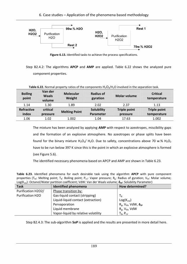
6. Case studies – Application of the phenomena based methodology
189
Figure 6.13. Identified tasks to achieve the process specifications.
Step B2.4.2: The algorithms APCP and AMP are applied. Table 6.22 shows the analyzed pure
component properties.
Table 6.22. Normal property ratios of the components H2O2/H2O involved in the separation task.
Boiling point
Van der Waals
volume
Molecular Weight
Radius of gyration Molar volume Critical
temperature
1.14 1.30 1.89 2.02 2.37 1.13 Refractive
index critical
pressure Melting Point Solubility Parameter
Triple point pressure
Triple point temperature
1.06 1.02 1.002 1.04 17.63 1.002
The mixture has been analyzed by applying AMP with respect to azeotropes, miscibility gaps
and the formation of an explosive atmosphere. No azeotropes or phase splits have been
found for the binary mixture H2O2/ H2O. Due to safety, concentrations above 70 w.% H2O2
have to be run below 397 K since this is the point in which an explosive atmosphere is formed
(see Figure 5.6).
The identified necessary phenomena based on APCP and AMP are shown in Table 6.23.
Table 6.23. Identified phenomena for each desirable task using the algorithm APCP with pure component properties (TM: Melting point; TB: Boiling point; PLV: Vapor pressure; Rg: Radius of gyration; VM: Molar volume; Log(Kow): Octanol/Water partition coefficient; VdW: Van der Waals volume; SP: Solubility Parameter) Task Identified phenomena How determined? Purification H2O2/ Purification H2O
Phase transition by: Gas-liquid contact (stripping) Liquid-liquid contact (extraction) Pervaporation Liquid membrane Vapor-liquid by relative volatility
TB Log(Kow) Rg, VM, VdW, SP Rg, VM, VdW TB, PLV
Step B2.4.3: The sub-algorithm SoP is applied and the results are presented in more detail here.
219
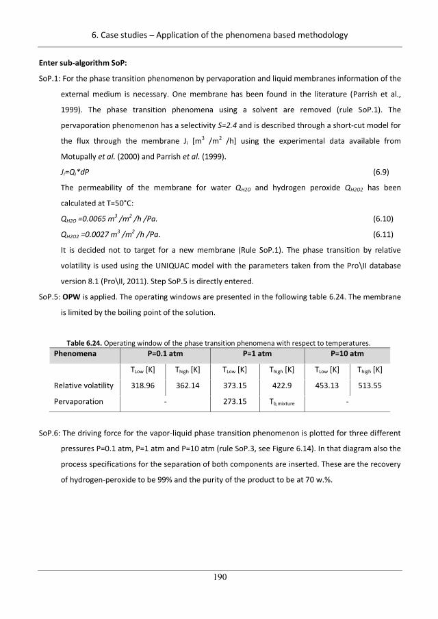
6. Case studies – Application of the phenomena based methodology
190
Enter sub-algorithm SoP:
SoP.1: For the phase transition phenomenon by pervaporation and liquid membranes information of the
external medium is necessary. One membrane has been found in the literature (Parrish et al.,
1999). The phase transition phenomena using a solvent are removed (rule SoP.1). The
pervaporation phenomenon has a selectivity S=2.4 and is described through a short-cut model for
the flux through the membrane Ji [m3 /m2 /h] using the experimental data available from
Motupally et al. (2000) and Parrish et al. (1999).
Ji=Qi*dP (6.9)
The permeability of the membrane for water QH2O and hydrogen peroxide QH2O2 has been
calculated at T=50°C:
QH2O =0.0065 m3 /m2 /h /Pa. (6.10)
QH2O2 =0.0027 m3 /m2 /h /Pa. (6.11)
It is decided not to target for a new membrane (Rule SoP.1). The phase transition by relative
volatility is used using the UNIQUAC model with the parameters taken from the Pro\II database
version 8.1 (Pro\II, 2011). Step SoP.5 is directly entered.
SoP.5: OPW is applied. The operating windows are presented in the following table 6.24. The membrane
is limited by the boiling point of the solution.
Table 6.24. Operating window of the phase transition phenomena with respect to temperatures. Phenomena P=0.1 atm P=1 atm P=10 atm
TLow [K] Thigh [K] TLow [K] Thigh [K] TLow [K] Thigh [K]
Relative volatility 318.96 362.14 373.15 422.9 453.13 513.55
Pervaporation - 273.15 Tb,mixture -
SoP.6: The driving force for the vapor-liquid phase transition phenomenon is plotted for three different
pressures P=0.1 atm, P=1 atm and P=10 atm (rule SoP.3, see Figure 6.14). In that diagram also the
process specifications for the separation of both components are inserted. These are the recovery
of hydrogen-peroxide to be 99% and the purity of the product to be at 70 w.%.
220
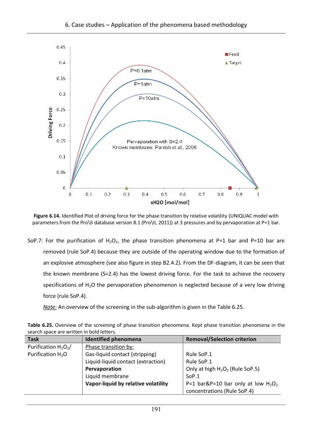
6. Case studies – Application of the phenomena based methodology
191
Figure 6.14. Identified Plot of driving force for the phase transition by relative volatility (UNIQUAC model with
parameters from the Pro\II database version 8.1 (Pro\II, 2011)) at 3 pressures and by pervaporation at P=1 bar.
SoP.7: For the purification of H2O2, the phase transition phenomena at P=1 bar and P=10 bar are
removed (rule SoP.4) because they are outside of the operating window due to the formation of
an explosive atmosphere (see also figure in step B2.4.2). From the DF-diagram, it can be seen that
the known membrane (S=2.4) has the lowest driving force. For the task to achieve the recovery
specifications of H2O the pervaporation phenomenon is neglected because of a very low driving
force (rule SoP.4).
Note: An overview of the screening in the sub-algorithm is given in the Table 6.25.
Table 6.25. Overview of the screening of phase transition phenomena. Kept phase transition phenomena in the search space are written in bold letters. Task Identified phenomena Removal/Selection criterion Purification H2O2/ Purification H2O
Phase transition by: Gas-liquid contact (stripping) Liquid-liquid contact (extraction) Pervaporation Liquid membrane Vapor-liquid by relative volatility
Rule SoP.1 Rule SoP.1 Only at high H2O2 (Rule SoP.5) SoP.1 P=1 bar&P=10 bar only at low H2O2 concentrations (Rule SoP.4)
221
6. Case studies – Application of the phenomena based methodology
192
SoP.8: All tasks can be fulfilled. No additional tasks are identified in this step. Step B2.4.4 is entered
Exit sub-algorithm SoP
Step B2.4.4: No physical limitation in the design is found.
Step B2.5: No additional necessary tasks are identified (Rules B2.14-B2.15).
Step B2.6: Step P3 is entered.
6.2.3. Step P3: Identification of desirable phenomena
Step P3.1: Identify additional desirable tasks for enhancement of the necessary ones
Step P3.1.1: The list of keywords KPI for identification of PI possibilities includes the task and the
objective function.
Step P3.1.2-P3.1.3: No additional tasks are identified.
Step P3.2-P3.5: The steps are not necessary since output of step P3.1.3 is zero.
Step P3.6: Identify accompanying phenomena by contacting the knowledge base for each identified
phenomenon: In total 15 phenomena (nP,tot=15.) are identified which are presented in the
appendix A.11 (see Table A.28).
Step P3.7: The algorithm OPW is applied to determine the operating window of each phenomenon (see
Table 6.26).
222
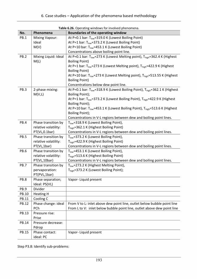
6. Case studies – Application of the phenomena based methodology
193
Table 6.26. Operating windows for involved phenomena. No. Phenomena Boundaries of the operating window PB.1 Mixing Vapour:
Ideal M(V)
At P=0.1 bar: Tlow=319.0 K (Lowest Boiling Point) At P=1 bar: Tlow=373.2 K (Lowest Boiling Point) At P=10 bar: Tlow=453.1 K (Lowest Boiling Point) Concentrations above boiling point line.
PB.2 Mixing Liquid: Ideal M(L)
At P=0.1 bar: Tlow=273 K (Lowest Melting point), Thigh=362.4 K (Highest Boiling Point) At P=1 bar: Tlow=273 K (Lowest Melting point), Thigh=422.9 K (Highest Boiling Point) At P=10 bar: Tlow=273 K (Lowest Melting point), Thigh=513.55 K (Highest Boiling Point) Concentrations below dew point line.
PB.3 2-phase mixing: M(V,L)
At P=0.1 bar: Tlow=318.9 K (Lowest Boiling Point), Thigh=362.1 K (Highest Boiling Point); At P=1 bar: Tlow=373.2 K (Lowest Boiling Point), Thigh=422.9 K (Highest Boiling Point); At P=10 bar: Tlow=453.1 K (Lowest Boiling Point), Thigh=513.6 K (Highest Boiling Point); Concentrations in V-L regions between dew and boiling point lines.
PB.4 Phase transition by relative volatility: PT(VL,0.1bar)
Tlow=318.9 K (Lowest Boiling Point), Thigh=362.1 K (Highest Boiling Point) Concentrations in V-L regions between dew and boiling point lines.
PB.5 Phase transition by relative volatility: PT(VL,1bar)
Tlow=373.2 K (Lowest Boiling Point), Thigh=422.9 K (Highest Boiling Point) Concentrations in V-L regions between dew and boiling point lines.
PB.6 Phase transition by relative volatility: PT(VL,10bar)
Tlow=453.1 K (Lowest Boiling Point), Thigh=513.6 K (Highest Boiling Point) Concentrations in V-L regions between dew and boiling point lines.
PB.7 Phase transition by pervaporation: PT(PVL,1bar)
Tlow=273.2 K (Highest Melting Point), Thigh=373.2 K (Lowest Boiling Point);
PB.8 Phase separation; Ideal: PS(VL)
Vapor- Liquid present
PB.9 Divider PB.10 Heating H PB.11 Cooling C PB.12 Phase change: ideal
PCh From V to L: inlet above dew point line, outlet below bubble point line From L to V: inlet below bubble point line, outlet above dew point line
PB.13 Pressure rise: Prise
PB.14 Pressure decrease: Pdrop
PB.15 Phase contact: ideal: PC
Vapor- Liquid present
Step P3.8: Identify sub-problems:
223
6. Case studies – Application of the phenomena based methodology
194
Step P3.8.1: Only one sub-problem (SP=1) is identified in which all identified tasks are included
(rule P3.3).
Step P3.8.2: All tasks and corresponding phenomena are included into one list SP
6.2.4. Step P4: Generate feasible operation/flowsheet options
P4.1: Generate all feasible simultaneous phenomena building blocks SPB from the phenomena in the
search space:
P4.1.1: Identify the maximum number of phenomena within an SPB nP,max (Eq.6.12):
The number of competing phenomena is 8 because: Heating and cooling (1), pressurizing and
expanding (1), phase transition phenomena at different pressures (3) as well as phase change
and two-phase phenomena (1) and stream dividing (1) cannot be connected within one SPB.
Additionally, the dividing phenomenon is one SPB itself.
Hence, the maximum number of phenomena within a stage is nP,max=15-7=8.
P4.1.2: All possible SPB are generated using the connectivity rules. In total a number of 14913
(see Eq.6.12) SPB’s are generated.
,max
,max
1 , , /
1 !1 12911
1 ! !
PnP tot
k P tot w oD
nNSPB
n k k
(6.12)
P4.1.3: Screening of all SPB’s for feasibility: Using connectivity rules and the information of the
operating window of each phenomenon, a total number of 30 SPB’s is feasible which are
shown in Table 6.27.
224
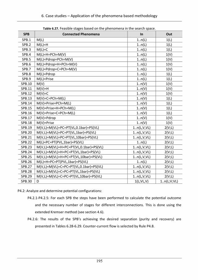
6. Case studies – Application of the phenomena based methodology
195
Table 6.27. Feasible stages based on the phenomena in the search space.
P4.2: Analyze and determine potential configurations:
P4.2.1-P4.2.5: For each SPB the steps have been performed to calculate the potential outcome
and the necessary number of stages for different interconnections. This is done using the
extended Kremser method (see section 4.6).
P4.2.6: The results of the SPB’s achieving the desired separation (purity and recovery) are
presented in Tables 6.28-6.29. Counter-current flow is selected by Rule P4.8.
SPB Connected Phenomena In Out SPB.1 M(L) 1..n(L) 1(L) SPB.2 M(L)=H 1..n(L) 1(L) SPB.3 M(L)=C 1..n(L) 1(L) SPB.4 M(L)=H=PCh=M(V) 1..n(L) 1(V) SPB.5 M(L)=Pdrop=PCh=M(V) 1..n(L) 1(V) SPB.6 M(L)=Pdrop=H=PCh=M(V) 1..n(L) 1(V) SPB.7 M(L)=Pdrop=C=PCh=M(V) 1..n(L) 1(V) SPB.8 M(L)=Pdrop 1..n(L) 1(L) SPB.9 M(L)=Prise 1..n(L) 1(L)
SPB.10 M(V) 1..n(V) 1(V) SPB.11 M(V)=H 1..n(V) 1(V) SPB.12 M(V)=C 1..n(V) 1(V) SPB.13 M(V)=C=PCh=M(L) 1..n(V) 1(L) SPB.14 M(V)=Prise=PCh=M(L) 1..n(V) 1(L) SPB.15 M(V)=Prise=H=PCh=M(L) 1..n(V) 1(L) SPB.16 M(V)=Prise=C=PCh=M(L) 1..n(V) 1(L) SPB.17 M(V)=Pdrop 1..n(V) 1(V) SPB.18 M(V)=Prise 1..n(V) 1(V) SPB.19 M(V,L)=M(VL)=PC=PT(VL,0.1bar)=PS(VL) 1..n(L,V,VL) 2(V;L) SPB.20 M(V,L)=M(VL)=PC=PT(VL,1bar)=PS(VL) 1..n(L,V,VL) 2(V;L) SPB.21 M(V,L)=M(VL)=PC=PT(VL,10bar)=PS(VL) 1..n(L,V,VL) 2(V;L) SPB.22 M(L)=PC=PT(PVL,1bar)=PS(VL) 1..n(L) 2(V;L) SPB.23 M(V,L)=M(VL)=H=PC=PT(VL,0.1bar)=PS(VL) 1..n(L,V,VL) 2(V;L) SPB.24 M(V,L)=M(VL)=H=PC=PT(VL,1bar)=PS(VL) 1..n(L,V,VL) 2(V;L) SPB.25 M(V,L)=M(VL)=H=PC=PT(VL,10bar)=PS(VL) 1..n(L,V,VL) 2(V;L) SPB.26 M(L)=H=PC=PT(PVL,1bar)=PS(VL) 1..n(L) 2(V;L) SPB.27 M(V,L)=M(VL)=C=PC=PT(VL,0.1bar)=PS(VL) 1..n(L,V,VL) 2(V;L) SPB.28 M(V,L)=M(VL)=C=PC=PT(VL,1bar)=PS(VL) 1..n(L,V,VL) 2(V;L) SPB.29 M(V,L)=M(VL)=C=PC=PT(VL,10bar)=PS(VL) 1..n(L,V,VL) 2(V;L) SPB.30 D 1(L;VL,V) 1..n(L;V;VL)
225
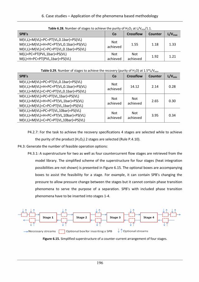
6. Case studies – Application of the phenomena based methodology
196
Table 6.28. Number of stages to achieve the purity of H2O2 at L/Vmin/1.1.
Table 0.29. Number of stages to achieve the recovery (purity of H2O) at 1.5*L/Vmin.
P4.2.7: For the task to achieve the recovery specifications 4 stages are selected while to achieve
the purity of the product (H2O2) 2 stages are selected (Rule P.4.10).
P4.3: Generate the number of feasible operation options:
P4.3.1: A superstructure for two as well as four countercurrent flow stages are retrieved from the
model library. The simplified scheme of the superstructure for four stages (heat integration
possibilities are not shown) is presented in Figure 6.15. The optional boxes are accompanying
boxes to assist the feasibility for a stage. For example, it can contain SPB’s changing the
pressure to allow pressure change between the stages but it cannot contain phase transition
phenomena to serve the purpose of a separation. SPB’s with included phase transition
phenomena have to be inserted into stages 1-4.
Figure 6.15. Simplified superstructure of a counter-current arrangement of four stages.
SPB’s Co Crossflow Counter L/Vmax M(V,L)=M(VL)=PC=PT(VL,0.1bar)=PS(VL) M(V,L)=M(VL)=H=PC=PT(VL,0.1bar)=PS(VL) M(V,L)=M(VL)=C=PC=PT(VL,0.1bar)=PS(VL)
Not achieved 1.55 1.18 1.33
M(L)=PC=PT(PVL,1bar)=PS(VL) M(L)=H=PC=PT(PVL,1bar)=PS(VL)
Not achieved
Not achieved 1.92 1.21
SPB’s Co Crossflow Counter L/Vmin M(V,L)=M(VL)=PC=PT(VL,0.1bar)=PS(VL) M(V,L)=M(VL)=H=PC=PT(VL,0.1bar)=PS(VL) M(V,L)=M(VL)=C=PC=PT(VL,0.1bar)=PS(VL)
Not achieved 14.12 2.14 0.28
M(V,L)=M(VL)=PC=PT(VL,1bar)=PS(VL) M(V,L)=M(VL)=H=PC=PT(VL,1bar)=PS(VL) M(V,L)=M(VL)=C=PC=PT(VL,1bar)=PS(VL)
Not achieved
Not achieved 2.65 0.30
M(V,L)=M(VL)=PC=PT(VL,10bar)=PS(VL) M(V,L)=M(VL)=H=PC=PT(VL,10bar)=PS(VL) M(V,L)=M(VL)=C=PC=PT(VL,10bar)=PS(VL)
Not achieved
Not achieved 3.95 0.34
226
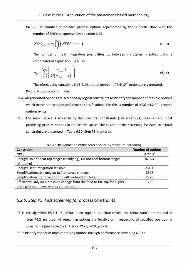
6. Case studies – Application of the phenomena based methodology
197
P4.3.2: The number of possible process options represented by this superstructure with the
number of SPB´s is expressed by equation 6.13.
,max
1
tasksstages task
nn
hiNOO n NSPB
(6.13)
The number of heat integration possibilities nhi between six stages is solved using a
combinatorial expression (Eq.6.14):
2
!! !
stagesnstages
hik stages
nn
k n k (6.14)
Therefore, using equations 6.13-6.14, a total number of 2.6·1010 options are generated.
P4.3.3: No reduction is made.
P4.4: All generated options are screened by logical constraints to identify the number of feasible options
which match the product and process specifications. For this, a number of NOOL=4.2·107 process
options exists.
P4.5. The search space is screened by the structural constraints (seeTable 6.21), leaving 1736 most
promising process options in the search space. The results of the screening for each structural
constraint are presented in Table 6.30. Step P5 is entered.
Table 6.30. Reduction of the search space by structural screening. Constraint Number of options NPOL 4.2·107 Energy: Do not heat top stages (rectifying), Do not cool bottom stages (stripping)
82944
Energy: Heat integration feasible 26100 Simplification: Use only up to 2 pressure changes 8352 Simplification: Remove options with redundant stages 2228 Efficiency: Only do a pressure change from the feed to the top for higher driving forces (lower energy consumption)
1736
6.2.5. Step P5: Fast screening for process constraints
P5.1: The algorithm P5.1.1-P5.1.4 has been applied. As initial values, the reflux ratio’s determined in
step P4.2 are used. All remaining options are feasible with respect to all specified operational
constraints (see Table 6.21). Hence NOOS= NOOO=1736.
P5.2: Identify the set of most promising options through performance screening NPOP:
227
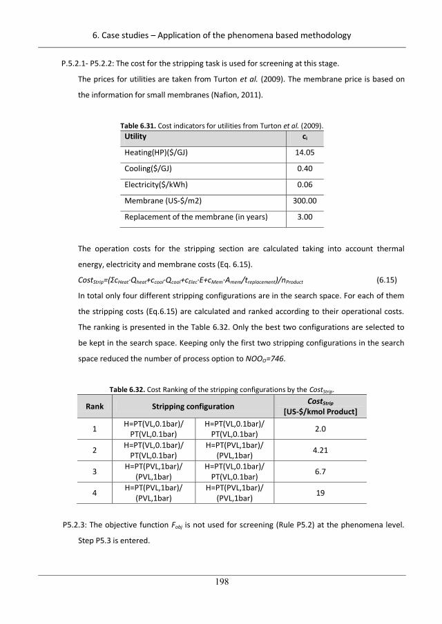
6. Case studies – Application of the phenomena based methodology
198
P.5.2.1- P5.2.2: The cost for the stripping task is used for screening at this stage.
The prices for utilities are taken from Turton et al. (2009). The membrane price is based on
the information for small membranes (Nafion, 2011).
Table 6.31. Cost indicators for utilities from Turton et al. (2009). Utility ci
Heating(HP)($/GJ) 14.05
Cooling($/GJ) 0.40
Electricity($/kWh) 0.06
Membrane (US-$/m2) 300.00
Replacement of the membrane (in years) 3.00
The operation costs for the stripping section are calculated taking into account thermal
energy, electricity and membrane costs (Eq. 6.15).
CostStrip=( cHeat·Qheat+ccool·Qcool+cElec·E+cMem·Amem/treplacement)/nProduct (6.15)
In total only four different stripping configurations are in the search space. For each of them
the stripping costs (Eq.6.15) are calculated and ranked according to their operational costs.
The ranking is presented in the Table 6.32. Only the best two configurations are selected to
be kept in the search space. Keeping only the first two stripping configurations in the search
space reduced the number of process option to NOOO=746.
Table 6.32. Cost Ranking of the stripping configurations by the CostStrip.
Rank Stripping configuration CostStrip [US-$/kmol Product]
1 H=PT(VL,0.1bar)/ PT(VL,0.1bar)
H=PT(VL,0.1bar)/ PT(VL,0.1bar) 2.0
2 H=PT(VL,0.1bar)/ PT(VL,0.1bar)
H=PT(PVL,1bar)/ (PVL,1bar) 4.21
3 H=PT(PVL,1bar)/ (PVL,1bar)
H=PT(VL,0.1bar)/ PT(VL,0.1bar) 6.7
4 H=PT(PVL,1bar)/ (PVL,1bar)
H=PT(PVL,1bar)/ (PVL,1bar) 19
P5.2.3: The objective function Fobj is not used for screening (Rule P5.2) at the phenomena level.
Step P5.3 is entered.
228
6. Case studies – Application of the phenomena based methodology
199
P5.3: Using the rules given in the knowledge-base: compressor/pump, heat-exchanger, column, reboiler,
condenser, flash, membrane separator and dividing wall column with/without heat exchange
between the separated zones are identified.
P5.4: The number of equipments in the process (NoE) is used as metric representing the capital costs for
screening at the unit operational level. Only 7 flowsheets are remaining in the search space
because they have the lowest number of unit operations in the fowsheet (less than 7 unit
operations). The 7 remaining options are shown in table 6.33.
Note: Process options #2,3,6 and 7 are internal heat integrated distillation columns at two
pressures in which the heat is transported from the rectifying to the stripping zone. Process
options #1 and 4 are heat integrated divided distillation columns at two pressures in which the
heat from the vapor leaving the rectifying section is used for the reboiler of the stripping zone. No
heat is transported from the rectifying to the stripping section in the column itself. Options #5-7
are hybrid operations of a distillation column and a pervaporation.
P5.5: All sub-problems SP have been solved, step 6 is entered (Rule P5.3). NOOP=NPOP.
229
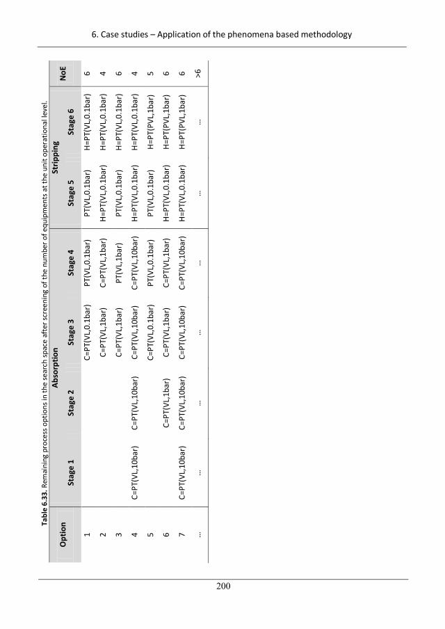
6. Case studies – Application of the phenomena based methodology
200
Tabl
e 6.
33. R
emai
ning
pro
cess
opt
ions
in th
e se
arch
spac
e af
ter s
cree
ning
of t
he n
umbe
r of e
quip
men
ts a
t the
uni
t ope
ratio
nal l
evel
.
Opt
ion
Abso
rptio
n St
rippi
ng
NoE
St
age
1 St
age
2 St
age
3 St
age
4 St
age
5 St
age
6
1
C=
PT(V
L,0.
1bar
) PT
(VL,
0.1b
ar)
PT(V
L,0.
1bar
) H=
PT(V
L,0.
1bar
) 6
2
C=
PT(V
L,1b
ar)
C=PT
(VL,
1bar
) H=
PT(V
L,0.
1bar
) H=
PT(V
L,0.
1bar
) 4
3
C=
PT(V
L,1b
ar)
PT(V
L,1b
ar)
PT(V
L,0.
1bar
) H=
PT(V
L,0.
1bar
) 6
4 C=
PT(V
L,10
bar)
C=
PT(V
L,10
bar)
C=
PT(V
L,10
bar)
C=
PT(V
L,10
bar)
H=
PT(V
L,0.
1bar
) H=
PT(V
L,0.
1bar
) 4
5
C=
PT(V
L,0.
1bar
) PT
(VL,
0.1b
ar)
PT(V
L,0.
1bar
) H=
PT(P
VL,1
bar)
5
6
C=PT
(VL,
1bar
) C=
PT(V
L,1b
ar)
C=PT
(VL,
1bar
) H=
PT(V
L,0.
1bar
) H=
PT(P
VL,1
bar)
6
7 C=
PT(V
L,10
bar)
C=
PT(V
L,10
bar)
C=
PT(V
L,10
bar)
C=
PT(V
L,10
bar)
H=
PT(V
L,0.
1bar
) H=
PT(P
VL,1
bar)
6
…
…
…
…
…
…
…
>6
230
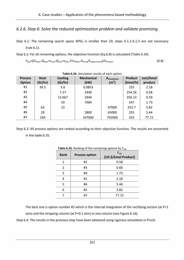
6. Case studies – Application of the phenomena based methodology
201
6.2.6. Step 6: Solve the reduced optimization problem and validate promising
Step 6.1: The remaining search space NPOP is smaller than 10, steps 6.1.1-6.1.3 are not necessary
(rule 6.1).
Step 6.2: For all remaining options, the objective function (Eq.6.8) is calculated (Table 6.34).
Fobj=( cHeat·Qheat+ccool·Qcool+cElec·E+cMem·Amem/treplacement)/nProduct (6.8)
Table 6.34. Simulation results of each option. Process Option
Heat (GJ/hr)
Cooling (GJ/hr)
Mechanical (kW)
Amembrane [m3]
Product [kmol/h]
cost/kmol product
#1 39.5 5.6 0.0853 255 2.18 #2 7.27 2440 254.26 0.58 #3 13.667 2440 256.13 0.59 #4 19 7004 247 1.73 #5 63 13 47000 253.7 5.82 #6 29 2800 65000 255 5.44 #7 249 107000 792000 255 77.72
Step 6.3: All process options are ranked according to their objective function. The results are presented
in the table 6.35.
Table 6.35. Ranking of the remaining options by Fobj.
The best one is option number #2 which is the internal integration of the rectifying section (at P=1
atm) and the stripping column (at P=0.1 atm) in one column (see Figure 6.16).
Step 6.4: The results in the previous step have been obtained using rigorous simulation in Pro\II.
Rank Process option Fobj [US-$/kmol Product]
1 #2 0.58 2 #3 0.60 3 #4 1.73 4 #1 2.18 5 #6 5.44 6 #5 5.82 7 #7 77.72
231
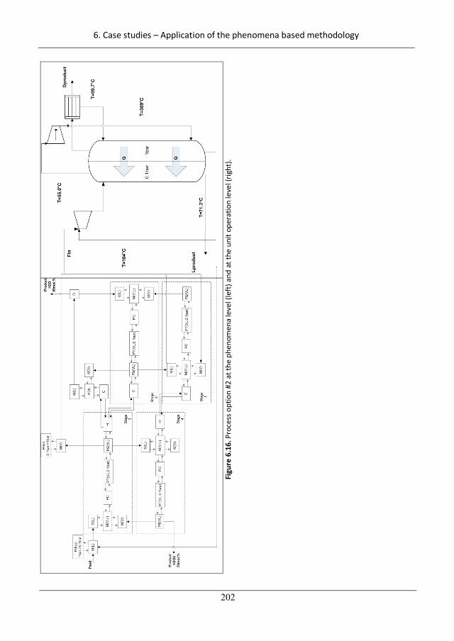
6. Case studies – Application of the phenomena based methodology
202
Figu
re 6
.16.
Pro
cess
opt
ion
#2 a
t the
phe
nom
ena
leve
l (le
ft) a
nd a
t the
uni
t ope
ratio
n le
vel (
right
).
232
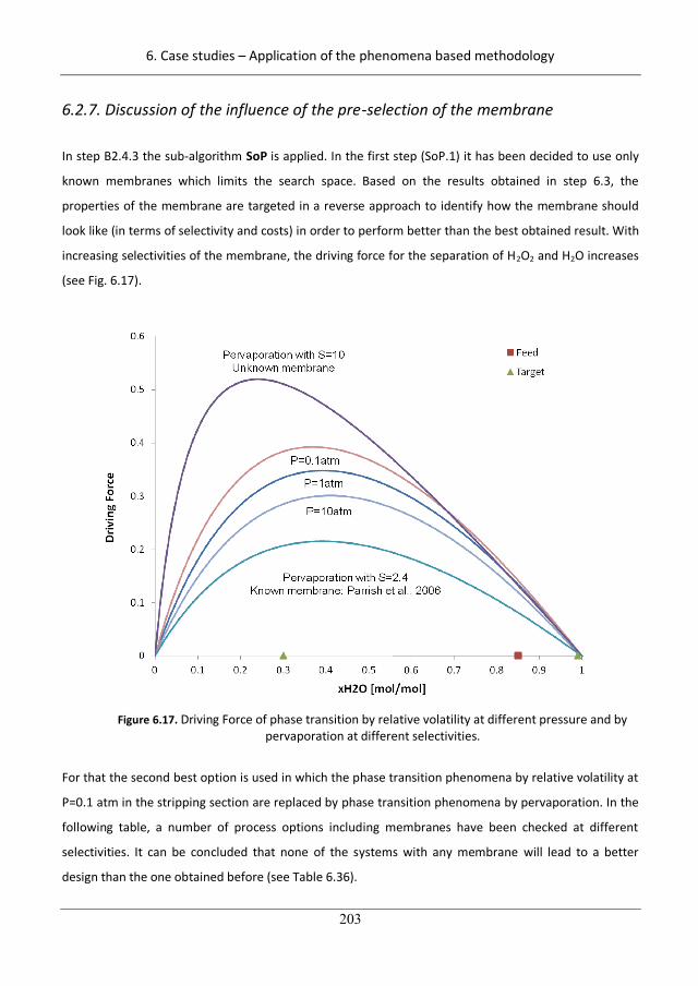
6. Case studies – Application of the phenomena based methodology
203
6.2.7. Discussion of the influence of the pre-selection of the membrane
In step B2.4.3 the sub-algorithm SoP is applied. In the first step (SoP.1) it has been decided to use only
known membranes which limits the search space. Based on the results obtained in step 6.3, the
properties of the membrane are targeted in a reverse approach to identify how the membrane should
look like (in terms of selectivity and costs) in order to perform better than the best obtained result. With
increasing selectivities of the membrane, the driving force for the separation of H2O2 and H2O increases
(see Fig. 6.17).
Figure 6.17. Driving Force of phase transition by relative volatility at different pressure and by
pervaporation at different selectivities.
For that the second best option is used in which the phase transition phenomena by relative volatility at
P=0.1 atm in the stripping section are replaced by phase transition phenomena by pervaporation. In the
following table, a number of process options including membranes have been checked at different
selectivities. It can be concluded that none of the systems with any membrane will lead to a better
design than the one obtained before (see Table 6.36).
233
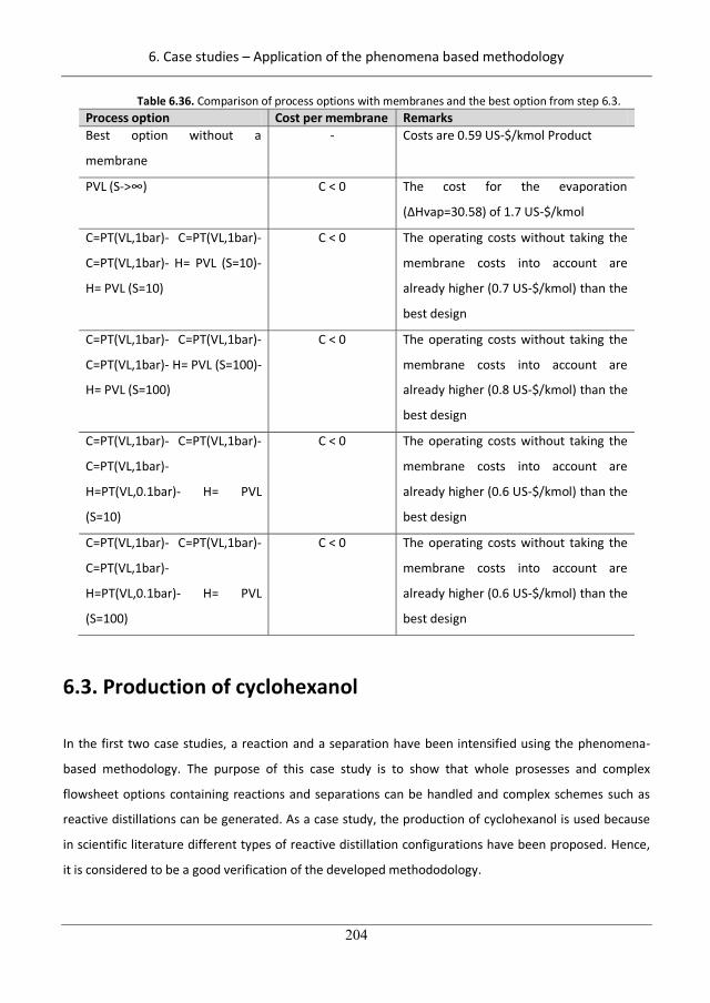
6. Case studies – Application of the phenomena based methodology
204
Table 6.36. Comparison of process options with membranes and the best option from step 6.3. Process option Cost per membrane Remarks Best option without a
membrane
- Costs are 0.59 US-$/kmol Product
PVL (S-> ) C < 0 The cost for the evaporation
( Hvap=30.58) of 1.7 US-$/kmol
C=PT(VL,1bar)- C=PT(VL,1bar)-
C=PT(VL,1bar)- H= PVL (S=10)-
H= PVL (S=10)
C < 0 The operating costs without taking the
membrane costs into account are
already higher (0.7 US-$/kmol) than the
best design
C=PT(VL,1bar)- C=PT(VL,1bar)-
C=PT(VL,1bar)- H= PVL (S=100)-
H= PVL (S=100)
C < 0 The operating costs without taking the
membrane costs into account are
already higher (0.8 US-$/kmol) than the
best design
C=PT(VL,1bar)- C=PT(VL,1bar)-
C=PT(VL,1bar)-
H=PT(VL,0.1bar)- H= PVL
(S=10)
C < 0 The operating costs without taking the
membrane costs into account are
already higher (0.6 US-$/kmol) than the
best design
C=PT(VL,1bar)- C=PT(VL,1bar)-
C=PT(VL,1bar)-
H=PT(VL,0.1bar)- H= PVL
(S=100)
C < 0 The operating costs without taking the
membrane costs into account are
already higher (0.6 US-$/kmol) than the
best design
6.3. Production of cyclohexanol
In the first two case studies, a reaction and a separation have been intensified using the phenomena-
based methodology. The purpose of this case study is to show that whole prosesses and complex
flowsheet options containing reactions and separations can be handled and complex schemes such as
reactive distillations can be generated. As a case study, the production of cyclohexanol is used because
in scientific literature different types of reactive distillation configurations have been proposed. Hence,
it is considered to be a good verification of the developed methododology.
234
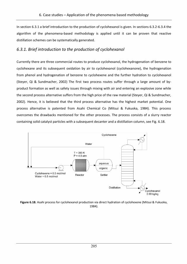
6. Case studies – Application of the phenomena based methodology
205
In section 6.3.1 a brief introduction to the production of cyclohexanol is given. In sections 6.3.2-6.3.4 the
algorithm of the phenomena-based methodology is applied until it can be proven that reactive
distillation schemes can be systematically generated.
6.3.1. Brief introduction to the production of cyclohexanol
Currently there are three commercial routes to produce cyclohexanol, the hydrogenation of benzene to
cyclohexane and its subsequent oxidation by air to cyclohexanol (cyclohexanone), the hydrogenation
from phenol and hydrogenation of benzene to cyclohexene and the further hydration to cyclohexanol
(Steyer, Qi & Sundmacher, 2002) The first two process routes suffer through a large amount of by-
product formation as well as safety issues through mixing with air and entering an explosive zone while
the second process alternative suffers from the high price of the raw material (Steyer, Qi & Sundmacher,
2002). Hence, it is believed that the third process alternative has the highest market potential. One
process alternative is patented from Asahi Chemical Co (Mitsui & Fukuoka, 1984). This process
overcomes the drawbacks mentioned for the other processes. The process consists of a slurry reactor
containing solid catalyst particles with a subsequent decanter and a distillation column, see Fig. 6.18.
Figure 6.18. Asahi process for cyclohexanol production via direct hydration of cyclohexene (Mitsui & Fukuoka, 1984).
235
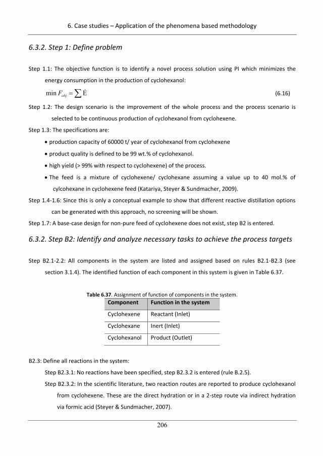
6. Case studies – Application of the phenomena based methodology
206
6.3.2. Step 1: Define problem
Step 1.1: The objective function is to identify a novel process solution using PI which minimizes the
energy consumption in the production of cyclohexanol:
min EobjF E (6.16)
Step 1.2: The design scenario is the improvement of the whole process and the process scenario is
selected to be continuous production of cyclohexanol from cyclohexene.
Step 1.3: The specifications are:
production capacity of 60000 t/ year of cyclohexanol from cyclohexene
product quality is defined to be 99 wt.% of cyclohexanol.
high yield (> 99% with respect to cyclohexene) of the process.
The feed is a mixture of cyclohexene/ cyclohexane assuming a value up to 40 mol.% of
cylcohexane in cyclohexene feed (Katariya, Steyer & Sundmacher, 2009).
Step 1.4-1.6: Since this is only a conceptual example to show that different reactive distillation options
can be generated with this approach, no screening will be shown.
Step 1.7: A base-case design for non-pure feed of cyclohexene does not exist, step B2 is entered.
6.3.2. Step B2: Identify and analyze necessary tasks to achieve the process targets
Step B2.1-2.2: All components in the system are listed and assigned based on rules B2.1-B2.3 (see
section 3.1.4). The identified function of each component in this system is given in Table 6.37.
Table 6.37. Assignment of function of components in the system. Component Function in the system
Cyclohexene Reactant (Inlet)
Cyclohexane Inert (Inlet)
Cyclohexanol Product (Outlet)
B2.3: Define all reactions in the system:
Step B2.3.1: No reactions have been specified, step B2.3.2 is entered (rule B.2.5).
Step B2.3.2: In the scientific literature, two reaction routes are reported to produce cyclohexanol
from cyclohexene. These are the direct hydration or in a 2-step route via indirect hydration
via formic acid (Steyer & Sundmacher, 2007).
236
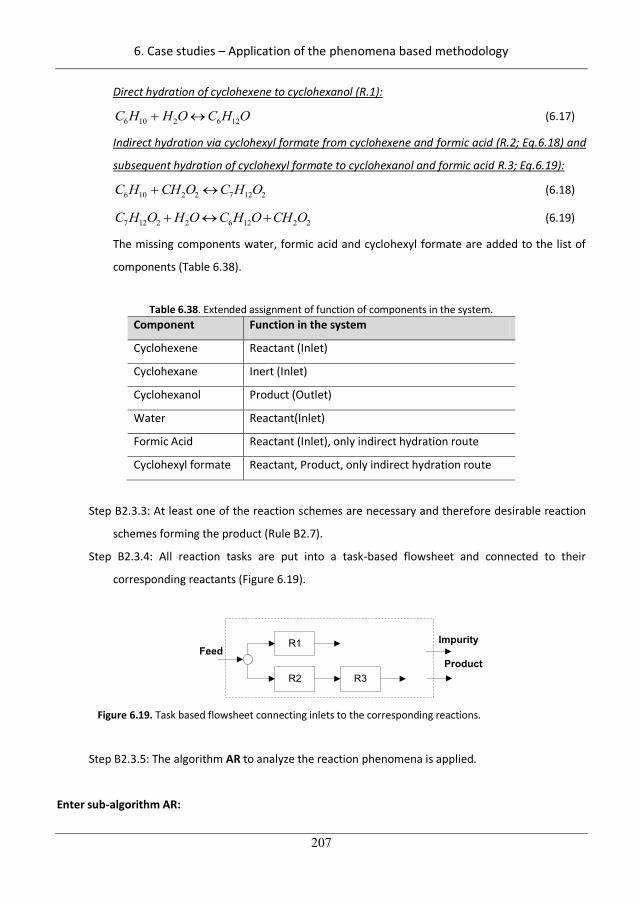
6. Case studies – Application of the phenomena based methodology
207
Direct hydration of cyclohexene to cyclohexanol (R.1):
6 10 2 6 12C H H O C H O (6.17)
Indirect hydration via cyclohexyl formate from cyclohexene and formic acid (R.2; Eq.6.18) and
subsequent hydration of cyclohexyl formate to cyclohexanol and formic acid R.3; Eq.6.19):
6 10 2 2 7 12 2C H CH O C H O (6.18)
7 12 2 2 6 12 2 2C H O H O C H O CH O (6.19)
The missing components water, formic acid and cyclohexyl formate are added to the list of
components (Table 6.38).
Table 6.38. Extended assignment of function of components in the system. Component Function in the system
Cyclohexene Reactant (Inlet)
Cyclohexane Inert (Inlet)
Cyclohexanol Product (Outlet)
Water Reactant(Inlet)
Formic Acid Reactant (Inlet), only indirect hydration route
Cyclohexyl formate Reactant, Product, only indirect hydration route
Step B2.3.3: At least one of the reaction schemes are necessary and therefore desirable reaction
schemes forming the product (Rule B2.7).
Step B2.3.4: All reaction tasks are put into a task-based flowsheet and connected to their
corresponding reactants (Figure 6.19).
FeedR1
R2 R3Product
Impurity
Figure 6.19. Task based flowsheet connecting inlets to the corresponding reactions.
Step B2.3.5: The algorithm AR to analyze the reaction phenomena is applied.
Enter sub-algorithm AR:
237
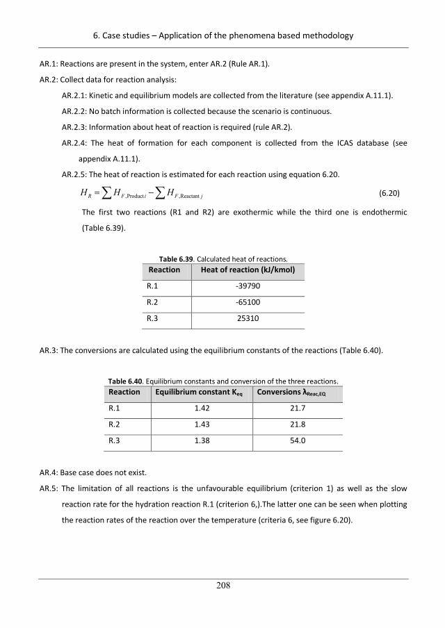
6. Case studies – Application of the phenomena based methodology
208
AR.1: Reactions are present in the system, enter AR.2 (Rule AR.1).
AR.2: Collect data for reaction analysis:
AR.2.1: Kinetic and equilibrium models are collected from the literature (see appendix A.11.1).
AR.2.2: No batch information is collected because the scenario is continuous.
AR.2.3: Information about heat of reaction is required (rule AR.2).
AR.2.4: The heat of formation for each component is collected from the ICAS database (see
appendix A.11.1).
AR.2.5: The heat of reaction is estimated for each reaction using equation 6.20.
,Product ,ReactantR F i F jH H H (6.20)
The first two reactions (R1 and R2) are exothermic while the third one is endothermic
(Table 6.39).
Table 6.39. Calculated heat of reactions. Reaction Heat of reaction (kJ/kmol)
R.1 -39790
R.2 -65100
R.3 25310
AR.3: The conversions are calculated using the equilibrium constants of the reactions (Table 6.40).
Table 6.40. Equilibrium constants and conversion of the three reactions. Reaction Equilibrium constant Keq Conversions Reac,EQ
R.1 1.42 21.7
R.2 1.43 21.8
R.3 1.38 54.0
AR.4: Base case does not exist.
AR.5: The limitation of all reactions is the unfavourable equilibrium (criterion 1) as well as the slow
reaction rate for the hydration reaction R.1 (criterion 6,).The latter one can be seen when plotting
the reaction rates of the reaction over the temperature (criteria 6, see figure 6.20).
238
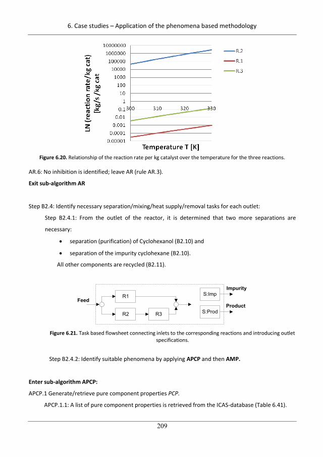
6. Case studies – Application of the phenomena based methodology
209
Figure 6.20. Relationship of the reaction rate per kg catalyst over the temperature for the three reactions.
AR.6: No inhibition is identified; leave AR (rule AR.3).
Exit sub-algorithm AR
Step B2.4: Identify necessary separation/mixing/heat supply/removal tasks for each outlet:
Step B2.4.1: From the outlet of the reactor, it is determined that two more separations are
necessary:
separation (purification) of Cyclohexanol (B2.10) and
separation of the impurity cyclohexane (B2.10).
All other components are recycled (B2.11).
ProductFeed
R1
R2 R3
Impurity
S:Prod
S:Imp
Figure 6.21. Task based flowsheet connecting inlets to the corresponding reactions and introducing outlet
specifications.
Step B2.4.2: Identify suitable phenomena by applying APCP and then AMP.
Enter sub-algorithm APCP:
APCP.1 Generate/retrieve pure component properties PCP.
APCP.1.1: A list of pure component properties is retrieved from the ICAS-database (Table 6.41).
239
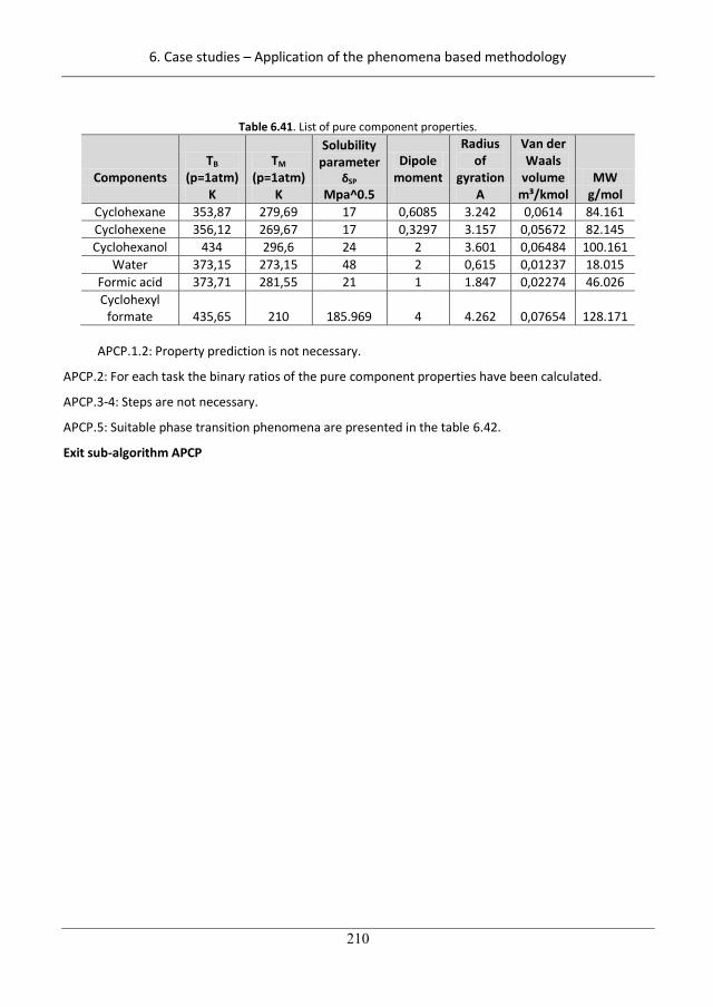
6. Case studies – Application of the phenomena based methodology
210
Table 6.41. List of pure component properties.
Components TB
(p=1atm) TM
(p=1atm)
Solubility parameter
SP Dipole
moment
Radius of
gyration
Van der Waals
volume MW K K Mpa^0.5 A m³/kmol g/mol
Cyclohexane 353,87 279,69 17 0,6085 3.242 0,0614 84.161 Cyclohexene 356,12 269,67 17 0,3297 3.157 0,05672 82.145 Cyclohexanol 434 296,6 24 2 3.601 0,06484 100.161
Water 373,15 273,15 48 2 0,615 0,01237 18.015 Formic acid 373,71 281,55 21 1 1.847 0,02274 46.026 Cyclohexyl
formate 435,65 210 185.969 4 4.262 0,07654 128.171 APCP.1.2: Property prediction is not necessary.
APCP.2: For each task the binary ratios of the pure component properties have been calculated.
APCP.3-4: Steps are not necessary.
APCP.5: Suitable phase transition phenomena are presented in the table 6.42.
Exit sub-algorithm APCP
240
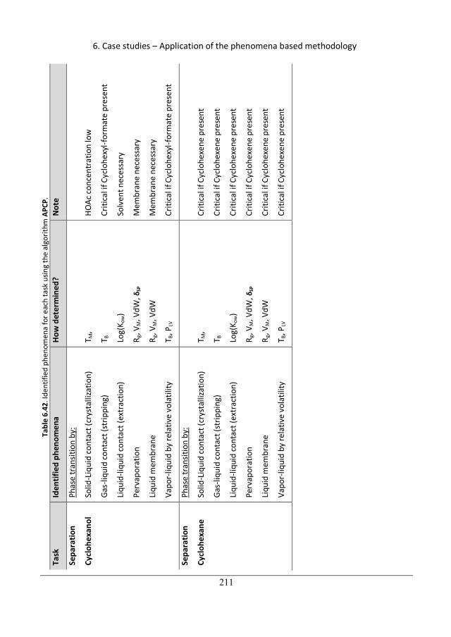
6. Case studies – Application of the phenomena based methodology
211
Tabl
e 6.
42. I
dent
ified
phe
nom
ena
for e
ach
task
usin
g th
e al
gorit
hm A
PCP.
Ta
sk
Iden
tifie
d ph
enom
ena
How
det
erm
ined
? N
ote
Sepa
ratio
n
Cycl
ohex
anol
Phas
e tr
ansit
ion
by:
Solid
-Liq
uid
cont
act (
crys
talli
zatio
n)
Gas-
liqui
d co
ntac
t (st
rippi
ng)
Liqu
id-li
quid
cont
act (
extr
actio
n)
Perv
apor
atio
n
Liqu
id m
embr
ane
Vapo
r-liq
uid
by re
lativ
e vo
latil
ity
T M,
T B
Log(
K ow
)
R g, V
M, V
dW,
SP
R g, V
M, V
dW
T B, P
LV
HOAc
conc
entr
atio
n lo
w
Criti
cal i
f Cyc
lohe
xyl-f
orm
ate
pres
ent
Solv
ent n
eces
sary
Mem
bran
e ne
cess
ary
Mem
bran
e ne
cess
ary
Criti
cal i
f Cyc
lohe
xyl-f
orm
ate
pres
ent
Sepa
ratio
n
Cycl
ohex
ane
Phas
e tr
ansit
ion
by:
Solid
-Liq
uid
cont
act (
crys
talli
zatio
n)
Gas-
liqui
d co
ntac
t (st
rippi
ng)
Liqu
id-li
quid
cont
act (
extr
actio
n)
Perv
apor
atio
n
Liqu
id m
embr
ane
Vapo
r-liq
uid
by re
lativ
e vo
latil
ity
T M,
T B
Log(
K ow
)
R g, V
M, V
dW,
SP
R g, V
M, V
dW
T B, P
LV
Criti
cal i
f Cyc
lohe
xene
pre
sent
Criti
cal i
f Cyc
lohe
xene
pre
sent
Criti
cal i
f Cyc
lohe
xene
pre
sent
Criti
cal i
f Cyc
lohe
xene
pre
sent
Criti
cal i
f Cyc
lohe
xene
pre
sent
Criti
cal i
f Cyc
lohe
xene
pre
sent
241
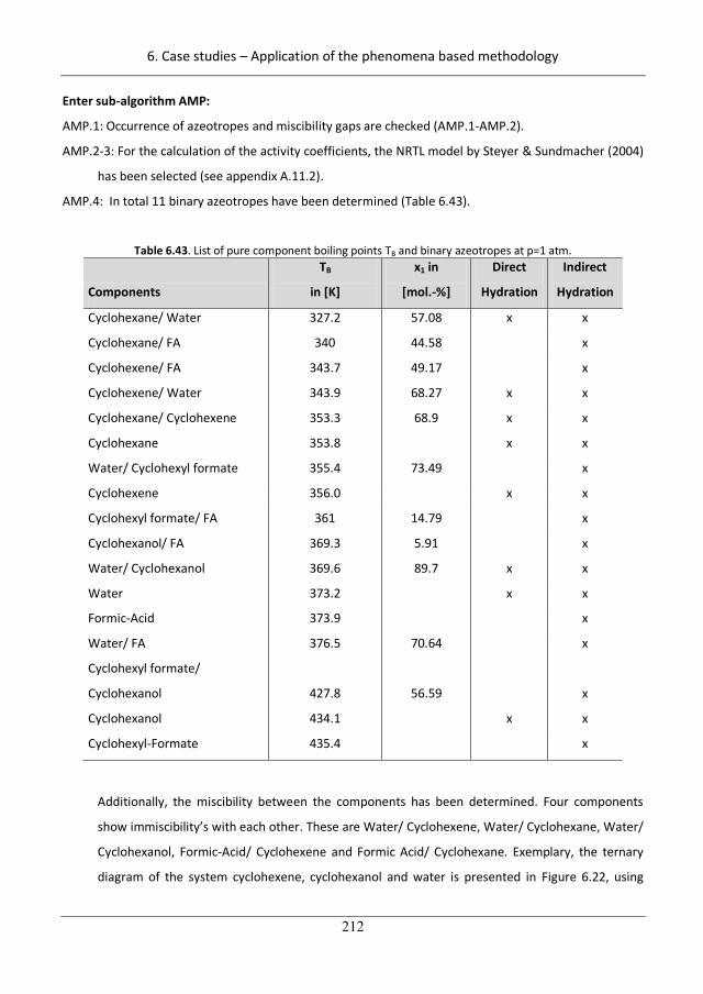
6. Case studies – Application of the phenomena based methodology
212
Enter sub-algorithm AMP:
AMP.1: Occurrence of azeotropes and miscibility gaps are checked (AMP.1-AMP.2).
AMP.2-3: For the calculation of the activity coefficients, the NRTL model by Steyer & Sundmacher (2004)
has been selected (see appendix A.11.2).
AMP.4: In total 11 binary azeotropes have been determined (Table 6.43).
Table 6.43. List of pure component boiling points TB and binary azeotropes at p=1 atm.
Components
TB
in [K]
x1 in
[mol.-%]
Direct
Hydration
Indirect
Hydration
Cyclohexane/ Water 327.2 57.08 x x
Cyclohexane/ FA 340 44.58 x
Cyclohexene/ FA 343.7 49.17 x
Cyclohexene/ Water 343.9 68.27 x x
Cyclohexane/ Cyclohexene 353.3 68.9 x x
Cyclohexane 353.8 x x
Water/ Cyclohexyl formate 355.4 73.49 x
Cyclohexene 356.0 x x
Cyclohexyl formate/ FA 361 14.79 x
Cyclohexanol/ FA 369.3 5.91 x
Water/ Cyclohexanol 369.6 89.7 x x
Water 373.2 x x
Formic-Acid 373.9 x
Water/ FA 376.5 70.64 x
Cyclohexyl formate/
Cyclohexanol 427.8 56.59 x
Cyclohexanol 434.1 x x
Cyclohexyl-Formate 435.4 x
Additionally, the miscibility between the components has been determined. Four components
show immiscibility’s with each other. These are Water/ Cyclohexene, Water/ Cyclohexane, Water/
Cyclohexanol, Formic-Acid/ Cyclohexene and Formic Acid/ Cyclohexane. Exemplary, the ternary
diagram of the system cyclohexene, cyclohexanol and water is presented in Figure 6.22, using
242
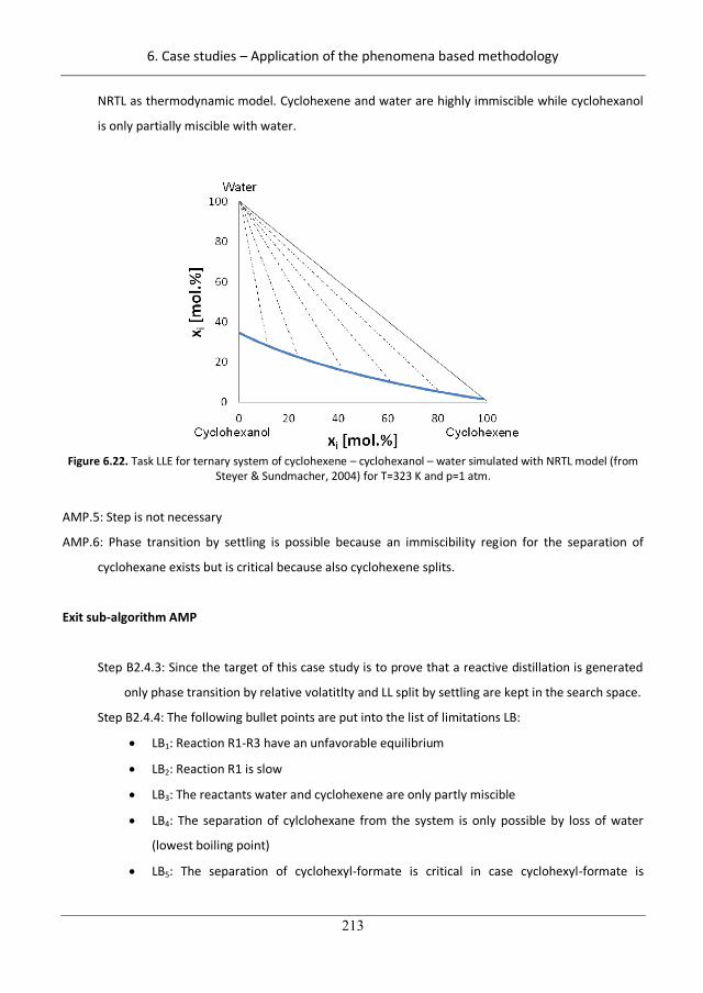
6. Case studies – Application of the phenomena based methodology
213
NRTL as thermodynamic model. Cyclohexene and water are highly immiscible while cyclohexanol
is only partially miscible with water.
Figure 6.22. Task LLE for ternary system of cyclohexene – cyclohexanol – water simulated with NRTL model (from
Steyer & Sundmacher, 2004) for T=323 K and p=1 atm.
AMP.5: Step is not necessary
AMP.6: Phase transition by settling is possible because an immiscibility region for the separation of
cyclohexane exists but is critical because also cyclohexene splits.
Exit sub-algorithm AMP
Step B2.4.3: Since the target of this case study is to prove that a reactive distillation is generated
only phase transition by relative volatitlty and LL split by settling are kept in the search space.
Step B2.4.4: The following bullet points are put into the list of limitations LB:
LB1: Reaction R1-R3 have an unfavorable equilibrium
LB2: Reaction R1 is slow
LB3: The reactants water and cyclohexene are only partly miscible
LB4: The separation of cylclohexane from the system is only possible by loss of water
(lowest boiling point)
LB5: The separation of cyclohexyl-formate is critical in case cyclohexyl-formate is
243
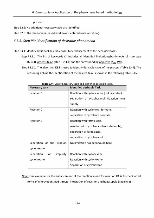
6. Case studies – Application of the phenomena based methodology
214
present.
Step B2.5: No additional necessary tasks are identified.
Step B2.6: The phenomena-based workflow is entered (rule workflow).
6.3.3. Step P3: Identification of desirable phenomena
Step P3.1: Identify additional desirable tasks for enhancement of the necessary tasks.
Step P3.1.1: The list of keywords KPI includes all identified limitations/bottlenecks LB (see step
B2.4.4), process tasks (step B.2.4.1) and the corresponding objective (Fobj, PM).
Step P3.1.2: The algorithm KBS is used to identify desirable tasks of the process (Table 6.44). The
reasoning behind the identification of the desired task is shown in the following table 6.45.
Table 6.44. List of necessary tasks and identified desirable tasks. Necessary task Identified desirable Task
Reaction 1 Reaction with cyclohexanol (not desirable),
separation of cyclohexanol, Reaction heat
supply
Reaction 2 Reaction with cyclohexyl-formate,
separation of cyclohexyl-formate
Reaction 3 Reaction with formic-acid,
reaction with cyclohexanol (not desirable),
separation of formic acid,
separation of cyclohexanol
Separation of the product:
cyclohexanol
No limitation has been found here.
Separation of impurity:
cyclohexane
Reaction with cyclohexane,
Reaction with cyclohexene,
Separation of cyclohexane
Note: One example for the enhancement of the reaction speed for reaction R1 is to check novel
forms of energy identified through integration of reaction and heat supply (Table 6.45).
244
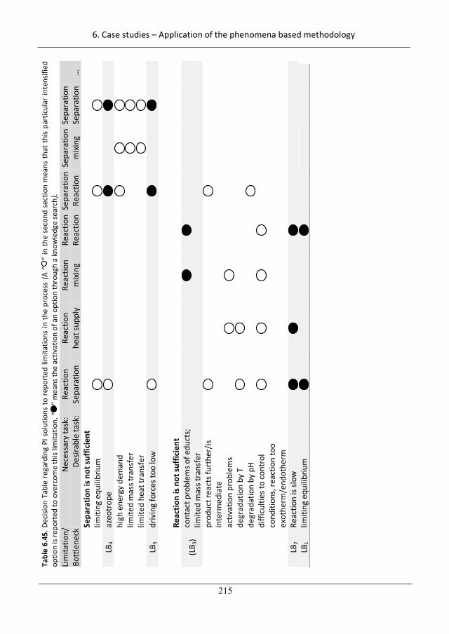
6. Case studies – Application of the phenomena based methodology
215
Tabl
e 6.
45. D
ecisi
on T
able
reg
ardi
ng P
I sol
utio
ns t
o re
port
ed li
mita
tions
in t
he p
roce
ss (
A “
” in
the
sec
ond
sect
ion
mea
ns t
hat
this
part
icul
ar in
tens
ified
op
tion
is re
port
ed to
ove
rcom
e th
is lim
itatio
n, “
” m
eans
the
activ
atio
n of
an
optio
n th
roug
h a
know
ledg
e se
arch
). Li
mita
tion/
Bo
ttle
neck
N
eces
sary
task
: De
sirab
le ta
sk:
Reac
tion
Sepa
ratio
n Re
actio
n
heat
supp
ly
Reac
tion
mix
ing
Reac
tion
Reac
tion
Sepa
ratio
n Re
actio
n Se
para
tion
mix
ing
Sepa
ratio
n Se
para
tion
…
Se
para
tion
is no
t suf
ficie
nt
lim
iting
equ
ilibr
ium
LB4
azeo
trop
e
high
ene
rgy
dem
and
lim
ited
mas
s tra
nsfe
r
limite
d he
at tr
ansf
er
LB5
driv
ing
forc
es to
o lo
w
Re
actio
n is
not s
uffic
ient
(LB 3
) co
ntac
t pro
blem
s of e
duct
s;
limite
d m
ass t
rans
fer
pr
oduc
t rea
cts f
urth
er/is
in
term
edia
te
ac
tivat
ion
prob
lem
s
degr
adat
ion
by T
degr
adat
ion
by p
H
di
fficu
lties
to co
ntro
l co
nditi
ons,
reac
tion
too
exot
herm
/end
othe
rm
LB2
Reac
tion
is slo
w
LB1
limiti
ng e
quili
briu
m
245
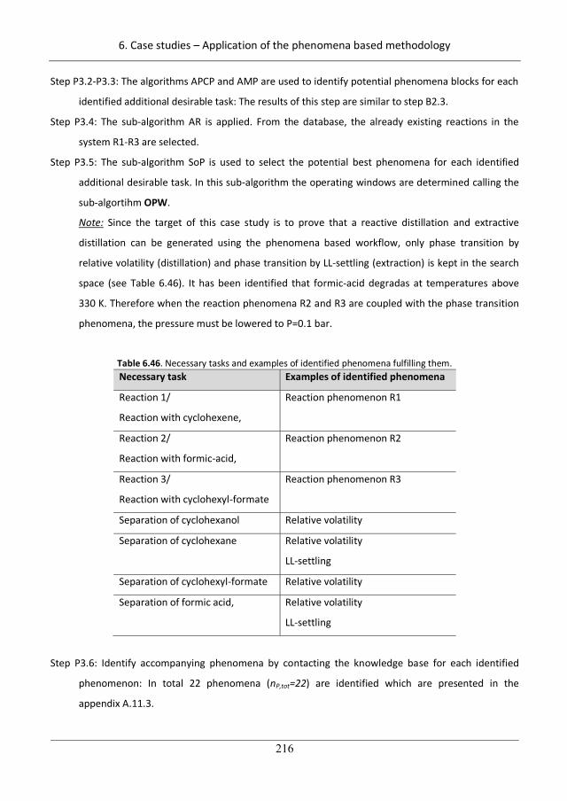
6. Case studies – Application of the phenomena based methodology
216
Step P3.2-P3.3: The algorithms APCP and AMP are used to identify potential phenomena blocks for each
identified additional desirable task: The results of this step are similar to step B2.3.
Step P3.4: The sub-algorithm AR is applied. From the database, the already existing reactions in the
system R1-R3 are selected.
Step P3.5: The sub-algorithm SoP is used to select the potential best phenomena for each identified
additional desirable task. In this sub-algorithm the operating windows are determined calling the
sub-algortihm OPW.
Note: Since the target of this case study is to prove that a reactive distillation and extractive
distillation can be generated using the phenomena based workflow, only phase transition by
relative volatility (distillation) and phase transition by LL-settling (extraction) is kept in the search
space (see Table 6.46). It has been identified that formic-acid degradas at temperatures above
330 K. Therefore when the reaction phenomena R2 and R3 are coupled with the phase transition
phenomena, the pressure must be lowered to P=0.1 bar.
Table 6.46. Necessary tasks and examples of identified phenomena fulfilling them. Necessary task Examples of identified phenomena
Reaction 1/
Reaction with cyclohexene,
Reaction phenomenon R1
Reaction 2/
Reaction with formic-acid,
Reaction phenomenon R2
Reaction 3/
Reaction with cyclohexyl-formate
Reaction phenomenon R3
Separation of cyclohexanol Relative volatility
Separation of cyclohexane Relative volatility
LL-settling
Separation of cyclohexyl-formate Relative volatility
Separation of formic acid,
Relative volatility
LL-settling
Step P3.6: Identify accompanying phenomena by contacting the knowledge base for each identified
phenomenon: In total 22 phenomena (nP,tot=22) are identified which are presented in the
appendix A.11.3.
246
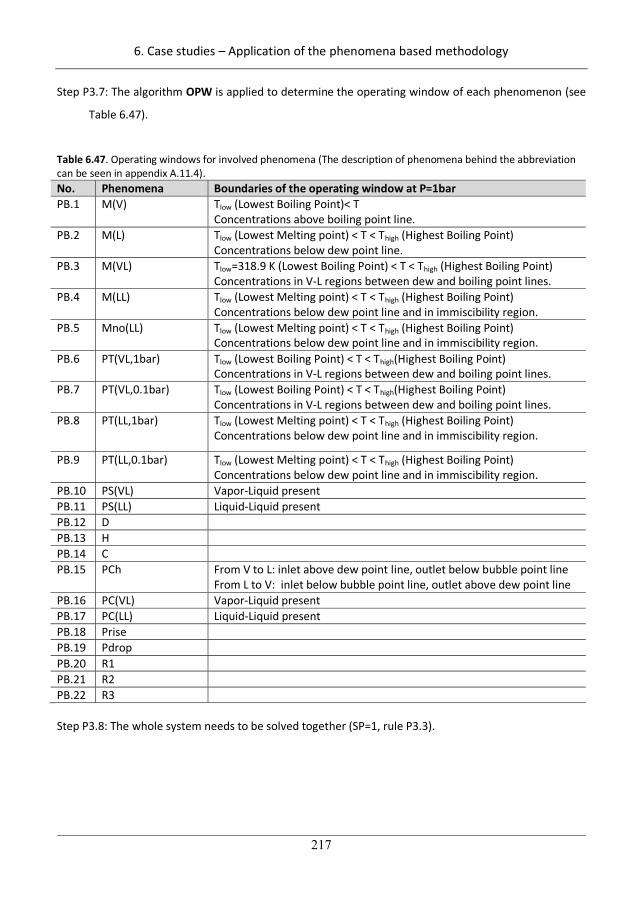
6. Case studies – Application of the phenomena based methodology
217
Step P3.7: The algorithm OPW is applied to determine the operating window of each phenomenon (see
Table 6.47).
Table 6.47. Operating windows for involved phenomena (The description of phenomena behind the abbreviation can be seen in appendix A.11.4). No. Phenomena Boundaries of the operating window at P=1bar PB.1 M(V) Tlow (Lowest Boiling Point)< T
Concentrations above boiling point line. PB.2 M(L) Tlow (Lowest Melting point) < T < Thigh (Highest Boiling Point)
Concentrations below dew point line. PB.3 M(VL) Tlow=318.9 K (Lowest Boiling Point) < T < Thigh (Highest Boiling Point)
Concentrations in V-L regions between dew and boiling point lines. PB.4 M(LL) Tlow (Lowest Melting point) < T < Thigh (Highest Boiling Point)
Concentrations below dew point line and in immiscibility region. PB.5 Mno(LL) Tlow (Lowest Melting point) < T < Thigh (Highest Boiling Point)
Concentrations below dew point line and in immiscibility region. PB.6 PT(VL,1bar)
Tlow (Lowest Boiling Point) < T < Thigh(Highest Boiling Point) Concentrations in V-L regions between dew and boiling point lines.
PB.7 PT(VL,0.1bar)
Tlow (Lowest Boiling Point) < T < Thigh(Highest Boiling Point) Concentrations in V-L regions between dew and boiling point lines.
PB.8 PT(LL,1bar) Tlow (Lowest Melting point) < T < Thigh (Highest Boiling Point) Concentrations below dew point line and in immiscibility region.
PB.9 PT(LL,0.1bar) Tlow (Lowest Melting point) < T < Thigh (Highest Boiling Point) Concentrations below dew point line and in immiscibility region.
PB.10 PS(VL) Vapor-Liquid present PB.11 PS(LL) Liquid-Liquid present PB.12 D PB.13 H PB.14 C PB.15 PCh From V to L: inlet above dew point line, outlet below bubble point line
From L to V: inlet below bubble point line, outlet above dew point line PB.16 PC(VL) Vapor-Liquid present PB.17 PC(LL) Liquid-Liquid present PB.18 Prise PB.19 Pdrop PB.20 R1 PB.21 R2 PB.22 R3 Step P3.8: The whole system needs to be solved together (SP=1, rule P3.3).
247
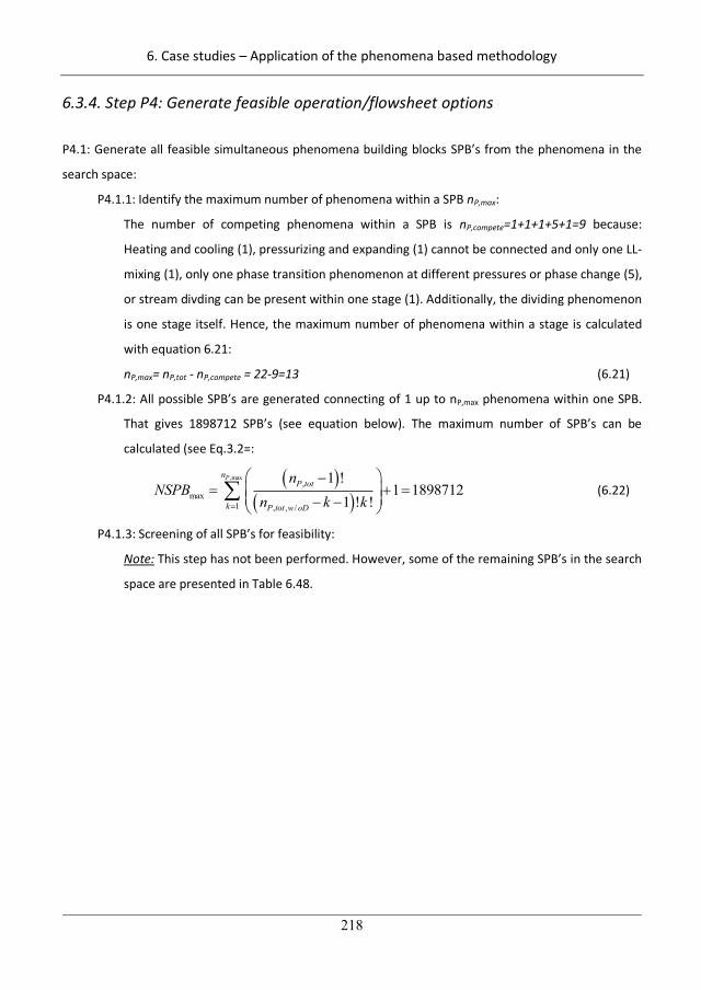
6. Case studies – Application of the phenomena based methodology
218
6.3.4. Step P4: Generate feasible operation/flowsheet options
P4.1: Generate all feasible simultaneous phenomena building blocks SPB’s from the phenomena in the
search space:
P4.1.1: Identify the maximum number of phenomena within a SPB nP,max:
The number of competing phenomena within a SPB is nP,compete=1+1+1+5+1=9 because:
Heating and cooling (1), pressurizing and expanding (1) cannot be connected and only one LL-
mixing (1), only one phase transition phenomenon at different pressures or phase change (5),
or stream divding can be present within one stage (1). Additionally, the dividing phenomenon
is one stage itself. Hence, the maximum number of phenomena within a stage is calculated
with equation 6.21:
nP,max= nP,tot - nP,compete = 22-9=13 (6.21)
P4.1.2: All possible SPB’s are generated connecting of 1 up to nP,max phenomena within one SPB.
That gives 1898712 SPB’s (see equation below). The maximum number of SPB’s can be
calculated (see Eq.3.2=:
,max
,max
1 , , /
1 !1 1898712
1 ! !
PnP tot
k P tot w oD
nNSPB
n k k (6.22)
P4.1.3: Screening of all SPB’s for feasibility:
Note: This step has not been performed. However, some of the remaining SPB’s in the search
space are presented in Table 6.48.
248
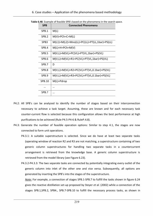
6. Case studies – Application of the phenomena based methodology
219
Table 6.48. Example of feasible SPB’s based on the phenomena in the search space. SPB Connected Phenomena
SPB.1 M(L)
SPB.2 M(V)=PCh=C=M(L)
SPB3 M(L1)=M(L2)=Mno(LL)=PC(LL)=PT(LL,1bar)=PS(LL)
SPB.4 M(L)=H=PCh=M(V)
SPB.5 M(V,L)=M(VL)=PC(VL)=PT(VL,1bar)=PS(VL)
SPB.6 M(V,L)=M(VL)=R1=PC(VL)=PT(VL,1bar)=PS(VL)
SPB.7 D
SPB.8 M(V,L)=M(VL)=R2=PC(VL)=PT(VL,0.1bar)=PS(VL)
SPB.9 M(V,L)=M(VL)=R3=PC(VL)=PT(VL,0.1bar)=PS(VL)
SPB.10 M(L)=Pdrop
… …
SPB.? …
P4.2: All SPB’s can be analyzed to identify the number of stages based on their interconnection
necessary to achieve a task target. Assuming, these are known and for each necessary task
counter-current flow is selected because this configuration allows the best performance at high
purifications to be achieved (Rule P4.5-P4-6 & RuleP.4.8).
P4.3: Generate the number of feasible operation options: Similar to step 4.1, the stages are now
connected to form unit operations.
P4.3.1: A suitable superstructure is selected. Since we do have at least two separate tasks
(operating window of reaction R2 and R3 are not matching, a superstructure containing of two
generic column superstructures for handling two separate tasks in a countercurrent
arrangement is retrieved from the knowledge base. A generic column superstructure is
retrieved from the model library (see Figure 6.23).
P4.3.2-P4.3.3: The two separate tasks are connected by potentially integrating every outlet of the
generic column into inlet of the other one and vice versa. Subsequently, all options are
generated by inserting the SPB’s into the stages of the superstructure.
Note: For example, a connection of stages SPB.1-SPB.7 to fulfill the tasks shown in figure 6.24
gives the reactive distillation set-up proposed by Steyer et al. (2002) while a connection of the
stages SPB.1,SPB.2, SPB4., SPB.7-SPB.10 to fulfill the necessary process tasks, as shown in
249
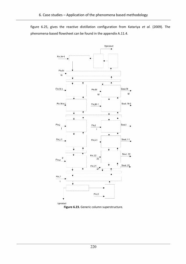
6. Case studies – Application of the phenomena based methodology
220
figure 6.25, gives the reactive distillation configuration from Katariya et al. (2009). The
phenomena-based flowsheet can be found in the appendix A.11.4.
Figure 6.23. Generic column superstructure.
250
6. Case studies – Application of the phenomena based methodology
221
Water,Cyclohexene/cyclohexane
Separationof cylcohexane by relative
volatility
Reaction R1
Separationof cylcohexane from water
by LL settling
Separationof cylcohexanol by relative
volatility
Separationof cylcohexanol by relative
volatility
cyclohexane
cyclohexanol
Unit-operation based Task based
Figure 6.24. Flowsheet for direct hydration based on unit operations (left; Steyer, Qi & Sundmacher, 2002) and based on phenomena here represented by the tasks (right).
251
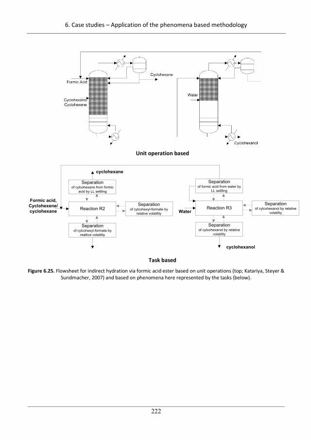
6. Case studies – Application of the phenomena based methodology
222
Unit operation based
Formic acid,Cyclohexene/cyclohexane Reaction R2
Separationof cylcohexane from formic
acid by LL settling
Separationof cylcohexyl-formate by
realtive volatility
Separationof cylcohexyl-formate by
relative volatility
cyclohexane
cyclohexanol
WaterReaction R3
Separationof formic acid from water by
LL settling
Separationof cylcohexanol by relative
volatility
Separationof cylcohexanol by relative
volatility
Task based
Figure 6.25. Flowsheet for indirect hydration via formic acid ester based on unit operations (top; Katariya, Steyer & Sundmacher, 2007) and based on phenomena here represented by the tasks (below).
252
7. Discussion
223
Chapter 7.
Discussion
In this PhD-project, a systematic synthesis/design methodology to achieve process intensification has
been developed. Two building blocks, that is PI unit-operations and phenomena have been considered
for solving the PI synthesis problem. The developed systematic PI synthesis/design methodology
provides the means to identify, to generate and to evaluate PI options, from which the optimal
intensified process option is obtained for the specified problem and the available data. The steps of the
PI-methodology follow a rationale which may be common sense and also independently developed by
others (PI Quick Scan process reviews in The Netherlands (van den Berg, 2001)). However, it has not
been established as a hybrid synthesis method to achieve PI in a whole process:
Using thermodynamic insights for the analysis of the process;
Using knowledge for the identification of potential PI unit operations and/or phenomena;
Using mathematical programming to identify the best feasible PI option from the set of
potential PI unit operations;
Generating PI solutions for a potentially quick implementation using the existing PI equipment;
Generating novel (not predefined, not develeloped) PI equipment processes using the
phenomena-based approach.
Hence, the scope of the developed methodology is beyond other PI synthesis methodologies (section 1,
illustrated in Figure 7.1.) because it supports the user to answer all questions arising during a process
synthesis problem (when; where; how/by which; why) on a quantitative basis, it includes a larger
number of considered PI equipment and it can be applied to the whole process.
Comparing the developed phenomena based approach with PI synthesis methods beyond unit-
operations, shows that the systematic way of identification of the PI solution covers other approaches at
other levels of aggregation. As illustration, the reasoning of the case study for the production of
cyclohexanol (case study 6.3) is compared with the reasoning by the application of the means-end
analysis for the methyl-acteate process by Siirola (1971-2011). Reactive distillation systems have been
proposed for both systems. Using, the phenomena based methodology, the unfavorable equilibrium in
the reaction is identified as main limitation as well as the necessity to overcome this limitation in the
reaction by coupling the reaction phenomenon with a suitable phase transition phenomenon. Since, all
253
7. Discussion
224
components can be fully or partially (in case of azeotropes) be separated using the same phase
transition phenomenon (relative volatility) the generated SPB’s show overlapping operating windows.
Whenever operating windows overlap for different phenomena, the phenomena can be connected or
integrated. Identifying a suitable counter-current flow arrangement using the Kremser method and
insertings SPB’s into the stages of this flow arrangement, reactive distillation systems have been
identified as a part of the solution search space. Now, the solution to the methyl-acetate production
using the means-ends analysis by Siirola (1971-2011) is briefly highlighted. All details to that case are
given in the appendix A.5. The identified equilibrium reaction task to form methyl-acetate does not run
until 100% conversion. Therefore, a number of separation tasks is identified to separate (and recycle)
the components in the system. All separation tasks can be separated using distillation-based
separations. Since these tasks follow the same separation principle (distillation) and their input/outputs
can be directly connected without temperature and/or pressure change, the tasks can be integrated into
one column. Comparing the means-ends analysis solution path by Siirola (1971-2011) for the methyl-
acetate example (see appendix A.5) with the phenomena based workflow solution path for the case
study to produce cyclohexanol (section 6.3) shows that the reasoning for identification and integration
are very similar. In fact, it can be concluded that the developed methodology in this PhD-thesis
integrates the solution of the means-ends analysis because the phenomena level is lower than the tasks
level (several different phenomena can fulfill one task in a process) and replaces the qualitative
reasoning as well as the expert knowledge analysis needed in the means-ends analysis by a systematic
generation and screening by quantitative measures (phenomena-based approach).
254
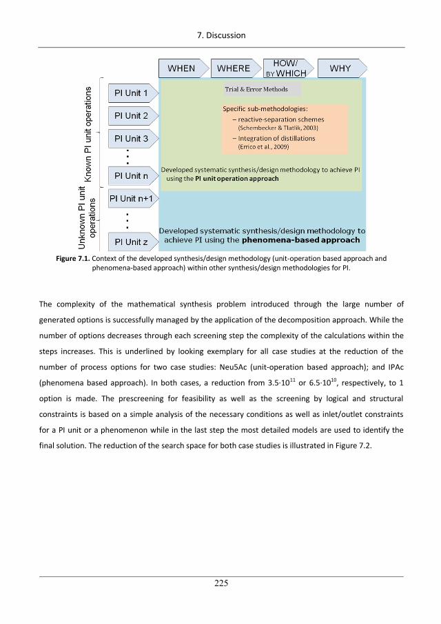
7. Discussion
225
Figure 7.1. Context of the developed synthesis/design methodology (unit-operation based approach and
phenomena-based approach) within other synthesis/design methodologies for PI.
The complexity of the mathematical synthesis problem introduced through the large number of
generated options is successfully managed by the application of the decomposition approach. While the
number of options decreases through each screening step the complexity of the calculations within the
steps increases. This is underlined by looking exemplary for all case studies at the reduction of the
number of process options for two case studies: Neu5Ac (unit-operation based approach); and IPAc
(phenomena based approach). In both cases, a reduction from 3.5·1011 or 6.5·1010, respectively, to 1
option is made. The prescreening for feasibility as well as the screening by logical and structural
constraints is based on a simple analysis of the necessary conditions as well as inlet/outlet constraints
for a PI unit or a phenomenon while in the last step the most detailed models are used to identify the
final solution. The reduction of the search space for both case studies is illustrated in Figure 7.2.
255
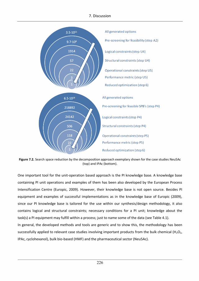
7. Discussion
226
Figure 7.2. Search space reduction by the decomposition approach exemplary shown for the case studies Neu5Ac
(top) and IPAc (bottom).
One important tool for the unit-operation based approach is the PI knowledge base. A knowledge base
containing PI unit operations and examples of them has been also developed by the European Process
Intensification Centre (Europic, 2009). However, their knowledge base is not open source. Besides PI
equipment and examples of successful implementations as in the knowledge base of Europic (2009),
since our PI knowledge base is tailored for the use within our synthesis/design methodology, it also
contains logical and structural constraints; necessary conditions for a PI unit; knowledge about the
task(s) a PI equipment may fulfill within a process; just to name some of the data (see Table 4.1).
In general, the developed methods and tools are generic and to show this, the methodology has been
successfully applied to relevant case studies involving important products from the bulk chemical (H2O2,
IPAc, cyclohexanol), bulk bio-based (HMF) and the pharmaceutical sector (Neu5Ac).
256
7. Discussion
227
The PI unit-operation workflow aims to push the implementation of already exisiting PI equipment while
the phenomena based approach aims to create novel PI process solutions beyond the ones currently
existing which potentially gives even larger improvement as for the unit-operation based approach. This
has been shown for the case study to purify H2O2 from an aqueous solution. However, the additional
expense for the phenomena-based approach are the increased complexity due to the larger number of
options as well as the increasing expected effort for the final implementation of the solution into a
process.
However, currently, the developed methodology based on the unit-operation approach is limited to:
PI equipment stored in the PI knowledge base:
Availability and reliability of models for PI units (often not available; for example for application
of microwaves);
Fixed reaction paths as input;
the manual handling of all the options.
The development of the phenomena-based approach has overcome the issues of the availability of
models (because they are developed as the synthesis is made) and the restriction to unit operations.
This also creates a new degree of complexity. However, it has been proven that the phenomena-based
methodology is capable to generate complex systems (IPAc case study for a new reactor, H2O2 for a new
separator) as well as to be applied to intensify whole processes (cyclohexanol). However, especially the
last case study (cyclohexanol) shows that the large number of options cannot be handled manually
anymore. An automation of the generation and screening in a software will be necessary.
The developed methodology based on the phenomena approach is limited to
Phenomena in the phenomena library;
Superstructures with fixed recycles (here, not all recycle possibilities have been enabled yet);
Limited number of rules for the identification of units from the phenomena based flowsheet;
The manual handling of all the options.
257

7. Discussion
228
258
8. Conclusions
229
Chapter 8.
Conclusions
8.1. Achievements
The work done within this thesis has resulted in the development of a systematic synthesis/design
methodology to achieve process intensification. This methodology allows the identification, generation
and evaluation of PI options in a search space, from which the optimal intensified process option is
obtained based on the specified synthesis problem and the available data. Process intensification using
the developed methodology can be achieved by using two different building blocks: PI unit operations
and phenomena. Within the methodology the following items have been achieved:
Managing the complexity of the generation of a potentially large number of process options and
based on this managing the complexity of solving the mathematical synthesis problem (section
2.1) by using a decomposition based solution approach. This approach has been successfully
transferred from the CAMD area for the systematic design of components and mixtures
(Karunanithi, Achenie & Gani, 2004). Through the decomposition approach, the mathematical PI
synthesis/design problem is decomposed into manageable sub-problems for an efficient
solution. That is simple calculations and simple analysis at early steps of the methodology for a
quick and efficient search space reduction and more complex calculations in later steps for the
identification of the best PI option.
Development of workflows which guide the user to generate the necessary information
necessary in each step to take decisions and to solve the specified PI synthesis/design problem
systematically.
Development of sub-algorithms for analysis of processes/phenomena based on pure
component properties, mixture properties, reaction properties; for the development of
superstructures; the selection of the best phenomena; the identification of operating windows
of unit operations as well as phenomena; to apply the knowledge base search, to do a model-
based search for process limitations of an existing process flowsheet for targeting PI.
Generation of PI processes using existing PI unit-operation for a potentially quick
implementation of the identified best PI process solution. For this a systematic classification of
259
8. Conclusions
230
purpose and characteristics of existing PI unit operations has been developed, Knowledge about
PI unit operations are stored in a knowledge base tool.
Development of a PI knowledge base tool for storage and retrieval of information of existing PI
unit operations which enables the use of existing PI unit operations as building blocks for the
methodology. The tool contains information such as: necessary conditions, tasks they fulfill in
the process, a potential list of limitations/bottlenecks to be overcome, etc., of around 110 PI
unit operations. The PI knowledge base is developed in such a way that it can be easily extended
through addition of additional columns (for new units) and rows (for new search classes). An
ontology and an efficient search algorithm allow the simple and quick retrieval of information.
Generation of novel process solution beyond existing PI unit-operation through the
development of a concept to synthesize processes by phenomena. This includes the
development and the definition of phenomena; a phenomena library for storage and retrieval of
phenomena; connectivity rules to interconnect phenomena to simultaneous phenomena
building blocks (SPB); connectivity rules to form unit operations from SPB’s; and connectivity
rules to form processes from unit-operations.
Development of superstructures to represent all process options in a search space.
Superstructures have been developed for the unit-operation based approach as well as the
phenomena based approach which are stored in a model library.
Embedment of existing tools from the PSE community into the methodology to
calculate/generate the desired target of a step. Integrated tools are the method based on
thermodynamic insights for analysis of the base-case design as well as identification of suitable
PI equipment and/or process phenomena; the driving force method for the identification of
suitable phenomena for a specific task; or the use of the element-based approach to generate
reactive-phase transition equilibrium curves necessary for evaluation of integration possibilities
of reaction and separation task
Development of a tool for quick and simple identification of the number of stages to achieve a
design specification of a process/task. This tool is based on the Kremser method which has been
extended to all kinds of phase transition phenomena as well as to integrated reactive phase
transition phenomena.
The development of a performance metric to evaluate PI on a quantitative basis. This metric
contains economic, safety, environmental as well as intrinsic intensified metrics.
260
8. Conclusions
231
The methodology together with the algorithms, tools and methods has been applied to six case studies.
For all of them, PI has been identified to improve the process in the specified target. The following
improvements have been achieved by PI using the unit-operation based approach:
The space-time-yield in the production of Neu5Ac (section 5.1) has been improved by a factor of
around 30. PI has been achieved by integrating of two reaction steps into a one-pot reactor
using better enzymes. Additionally, the production is realized in four processing steps
(compared to 7 in the base-case design).
The operational costs in the hydrogen peroxide production (section 5.2) process via the
anthraquinone route have been reduced by a factor of 2. PI has been achieved by replacing the
hydrogenator column through a microchannel reactor and integrating oxidation reaction and
extraction into a microchannel reactor-extractor. This allows a lower residence time of the
product and the solvent in the reactors which decreased the degradation and loss of product
and solvents. Additionally, the distillation column is replaced by a heat integrated distillation
column giving large savings in the energy costs.
In the production of HMF from fructose using water as solvent (section 5.3), the operational
costs have been decreased from around 7 US-$ to around 1.2 US-$. This has been achieved by
integrating reaction and subsequent extraction of the product into one microchannel device
using a better solvent. In the microchannel reactor-extractor a selectivity and a conversion of
the reaction of around 100% are potentially achieved. The costly downstream process for
purification in the base case design has been replaced by a heat-integrated distillation of the
product rather than distilling a large amount of water as in the base case design. This was
enabled since the new identified solvent has been selected to be a high boiling solvent.
Additionally, only two process steps are necessary for the production.
The following improvements have been identified by PI using the phenomena based approach:
For the production of isopropyl acetate (section 6.1), a novel intensified reactor solution has
been generated which is a tubular/rectangular millichannel reactor pervaporator (plate-and
frame concept). Comparing, this with existing reactive distillation concepts and the conventional
base case design, a decrease in the number of processing step, a decrease in the consumption of
heat, a decrease in the amount of catalysts, while increasing the conversion to 100% has been
realized.
In the the purification step (separation of hydrogen peroxide from water within the production
of hydrogen peroxide (section 6.2), the operational costs per kilogram product have been
261
8. Conclusions
232
reduced by a factor of 10. The best phenomena-based process solution is identified being a fully
heat integrated distillation column at two pressures.
In the production of cyclohexanol from cyclohexene and water (section 6.3), it has been shown
that all existing PI unit operation solutions (reactive distillation integrated with an extractor;
reactive distillation dividing wall columns) can be systematically generated. Besides a large
number of additional process options have been generated for intensifying the process.
8.2. Open challenges & future recommendations
The developed methodology depends on the reliability and availability of the models. For the unit-
operation based approach, these models are not always available and often not simple to develop since
the physical effect responsible for the achieved enhancement of a phenomenon (for example in case of
microwaves) is not always fully understood. This limits the current application of the unit operation
based approach.
Thorugh the case studies, it has been confirmed that often a limitation is occurring in or caused by the
reaction step. For example, hydrogen peroxide may also be produced from hydrogen and oxygen for
which small (intensified) units are necessary due to safety issues. Therefore, it may be beneficial to
couple the methodology with a tool which identifies all possible reaction routes. Currently, this tool
does not exist. Another valuable extension of the phenomena based methodology would be to decide
using a set of rules and the problem definition and/or indicators if a compartment, a series of units or a
battery (parallel units) is going to be developed. This would allow, in case of reactors for example, to
develop highly integrated unit concepts with locally (in all directions) different performances.
Up to now, the processes have been evaluated using the performance metric developed for PI and single
criterion objective functions. However, important more complex methods to evaluate sustainability such
as life cycle assessment (LCA) in which trade offs between different criteria are taken into account, have
not been considered so far.
Mass integration has been considered establishing fixed recycle streams in the superstructures for both,
the unit-operation based as well as the phenomena based approach. However, not all possible recycle
streams have been considered yet. However, recycles may be beneficial for improving the process
performance, for example of the overall conversion in a reaction process. However, how to evaluate and
integrate recycles at early steps into the methodology remains unsolved.
262
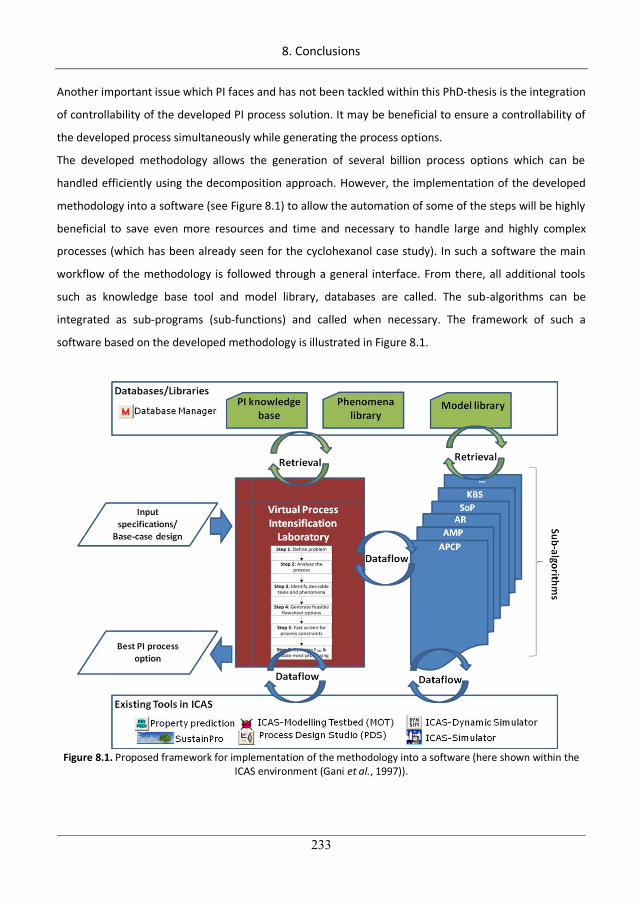
8. Conclusions
233
Another important issue which PI faces and has not been tackled within this PhD-thesis is the integration
of controllability of the developed PI process solution. It may be beneficial to ensure a controllability of
the developed process simultaneously while generating the process options.
The developed methodology allows the generation of several billion process options which can be
handled efficiently using the decomposition approach. However, the implementation of the developed
methodology into a software (see Figure 8.1) to allow the automation of some of the steps will be highly
beneficial to save even more resources and time and necessary to handle large and highly complex
processes (which has been already seen for the cyclohexanol case study). In such a software the main
workflow of the methodology is followed through a general interface. From there, all additional tools
such as knowledge base tool and model library, databases are called. The sub-algorithms can be
integrated as sub-programs (sub-functions) and called when necessary. The framework of such a
software based on the developed methodology is illustrated in Figure 8.1.
Figure 8.1. Proposed framework for implementation of the methodology into a software (here shown within the
ICAS environment (Gani et al., 1997)).
263

8. Conclusions
234
264
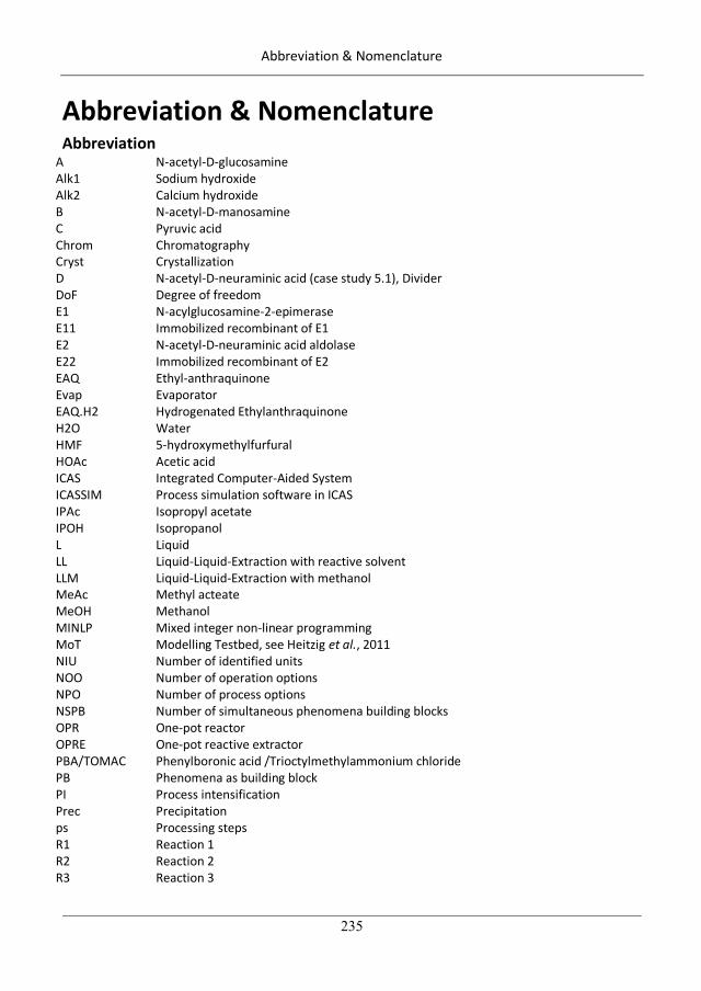
Abbreviation & Nomenclature
235
Abbreviation & Nomenclature Abbreviation
A N-acetyl-D-glucosamine Alk1 Sodium hydroxide Alk2 Calcium hydroxide B N-acetyl-D-manosamine C Pyruvic acid Chrom Chromatography Cryst Crystallization D N-acetyl-D-neuraminic acid (case study 5.1), Divider DoF Degree of freedom E1 N-acylglucosamine-2-epimerase E11 Immobilized recombinant of E1 E2 N-acetyl-D-neuraminic acid aldolase E22 Immobilized recombinant of E2 EAQ Ethyl-anthraquinone Evap Evaporator EAQ.H2 Hydrogenated Ethylanthraquinone H2O Water HMF 5-hydroxymethylfurfural HOAc Acetic acid ICAS Integrated Computer-Aided System ICASSIM Process simulation software in ICAS IPAc Isopropyl acetate IPOH Isopropanol L Liquid LL Liquid-Liquid-Extraction with reactive solvent LLM Liquid-Liquid-Extraction with methanol MeAc Methyl acteate MeOH Methanol MINLP Mixed integer non-linear programming MoT Modelling Testbed, see Heitzig et al., 2011 NIU Number of identified units NOO Number of operation options NPO Number of process options NSPB Number of simultaneous phenomena building blocks OPR One-pot reactor OPRE One-pot reactive extractor PBA/TOMAC Phenylboronic acid /Trioctylmethylammonium chloride PB Phenomena as building block PI Process intensification Prec Precipitation ps Processing steps R1 Reaction 1 R2 Reaction 2 R3 Reaction 3
265
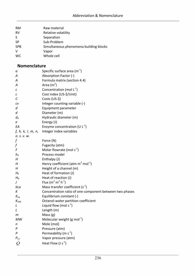
Abbreviation & Nomenclature
236
RM Raw material RV Relative volatility S Separation SP Sub-Problem SPB Simultaneous phenomena building blocks V Vapor WC Whole cell
Nomenclature
a Specific surface area (m-1) A Absorption-Factor (-) A Formula matrix (section 4.4) A Area (m2) c Concentration (mol L-1) c Cost index (US-$/Unit) C Costs (US-$) cv Integer counting variable (-) d Equipment parameter d Diameter (m) dh Hydraulic diameter (m) e Energy (J) EA Enzyme concentration (U L-1)f, h, k, l, m, n, o. s. v. w.
Integer index variables
f Force (N) f Fugacity (atm) F Molar flowrate (mol s-1) hP Process model H Enthalpy (J) H Henry coefficient (atm m3 mol-1) H Height of a channel (m) HF Heat of formation (J) HR Heat of reaction (J) J Flux (m3 m2 h-1) kLa Mass transfer coefficient (s-1) K Concentration ratio of one component between two phases Keq Equilibrium constant (-) KOW Octanol-water partition coefficient L Liquid flow (mol s-1) L Length (m) m Mass (g) MW Molecular weight (g mol-1) n Mole (mol) P Pressure (atm) P Permeability (m s-1) PLV Vapor pressure (atm) QQ Heat Flow (J s-1)
266
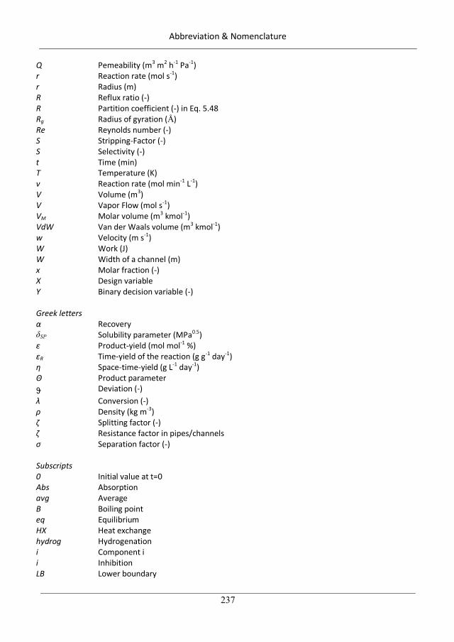
Abbreviation & Nomenclature
237
Q Pemeability (m3 m2 h-1 Pa-1) r Reaction rate (mol s-1) r Radius (m) R Reflux ratio (-) R Partition coefficient (-) in Eq. 5.48 Rg Radius of gyration (Å) Re Reynolds number (-) S Stripping-Factor (-) S Selectivity (-) t Time (min) T Temperature (K) v Reaction rate (mol min-1 L-1) V Volume (m3) V Vapor Flow (mol s-1) VM Molar volume (m3 kmol-1) VdW Van der Waals volume (m3 kmol-1) w Velocity (m s-1) W Work (J) W Width of a channel (m) x Molar fraction (-) X Design variable Y Binary decision variable (-) Greek letters
Recovery SP Solubility parameter (MPa0.5) Product-yield (mol mol-1 %) R Time-yield of the reaction (g g-1 day-1) Space-time-yield (g L-1 day-1) Product parameter
Deviation (-) Conversion (-) Density (kg m-3)
Splitting factor (-) Resistance factor in pipes/channels Separation factor (-)
Subscripts 0 Initial value at t=0 Abs Absorption avg Average B Boiling point eq Equilibrium HX Heat exchange hydrog Hydrogenation i Component i i Inhibition LB Lower boundary
267
Abbreviation & Nomenclature
238
M Melting point Mix Mixing, Mixer ox Oxidation P Product P Phenomenon Purif Purification of D R Reaction Str Stripping UB Upper boundary tot Total
Bottom outlet Top outlet
268
References
239
References
Algusane TY, Proios P, Georgiadis MC, Pistikopoulos EN. A framework for the synthesis of reactive absorption columns. Chem. Eng Process 2006; 45; 276-290.
Anxionnaz Z, Cabassud M, Gourdon C, Tochon P. Heat exchanger/ reactors (HEX reactors): concepts,
technologies: State-of-the-art. Chem Eng Process 2008;47:2029-2050.
Arizmendi-Sánchez J, Sharratt P. Phenomena-based modularisation of chemical process models to approach intensive options. Chem Eng J 2008; 135; 83-94.
Arpornwichanop A, Koomsup K, Assabumrungrat S. Hybrid reactive distillation for n-butyl acetate
production from dilute acetic acid. J Ind Eng Chem 2008; 14: 796-803.
Barnicki SD, Fair JR. Separation Systems Synthesis: A Knowledge-Based Approach. 1. Liquid Mixture
Separations. Ind Eng Chem Res 1990; 29(3):421-432.
Barnicki SD, Hoyme A, Siirola JJ. Separations Process Synthesis. In Kirk-Othmer Encyclopedia of Chemical Technology; Wiley & Sons; published online 19 May 2006.
Bauer K, Schembecker G. Synthese von Downstreamprozessen. Chem Ing Tech 2008; 80(1-2); 185-190.
Becht S, Franke R, Geißelmann A, Hahn H. An industrial view of process intensification. Chem Eng Process 2009; 329-332.
Bek-Pedersen E, Gani R. Design and synthesis of distillation systems using a driving-force-based approach. Chem Eng Process 2004; 43; 251-262.
Bessling B, Schembecker G, Simmrock KH. Design of processes with reactive distillation line diagrams.
Ind Eng Chem Res 1997; 36; 3032-3042.
Bicker M, Kaiser D, Vogel L. Dehydration of D-fructose to hydroxymethylfurfural in sub- and supercritical
fluids. J Supercrit Fluids 2005; 36; 118-126.
Biegler LT, Grossmann IE, Westerberg AW. Systematic Methods of Chemical Process Design, Prentice
Hall PTR, 1997.
Blayer S, Woodley JM, Dawson MJ, Lilly, MD. Alkaline biocatalysis for the direct synthesis of N-acetyl-D-
neuraminic acid (Neu5Ac) from N-acetyl-D-glucosamine (GlcNAc). Biotechnol Bioeng 1999;
66(2);131-136.
Boisen A, Christensen TB, Fu W, Gorbanev YY, Hansen TS, Jensen JS et al. Process integration for the
conversion of glucose to 2,5-furandicarboxylic acid. Chem Eng Res Des 2009; 87; 1318-1327.
269
References
240
Bozell JJ, Petersen GR. Technology development for the production of biobased products from
biorefinery carbohydrates – the US Department of Energy’s Top 10* revisited. Green Chem 2010;
12; 539-554.
Brueggemann S, Oldenburg J, Zhang P, Marquardt W. Robust dynamic simulation of three phase reactive
batch distillation columns. Ind Eng Chem Res 2004; 43; 3672-3684.
Buchaly C, Kreis P, Gorak A. Hybrid separation processes – Combination of reactive distillation with
membrane separation. Chem Eng Process 2007; 46: 790-799.
Cameron IT, Gani R. Product and Process Modelling: A Case Study Approach. 1st ed. Amsterdam:
Elsevier; 2011.
Cardenas-Guerra JC, Lopez-Arenas T, Lobo-Oehmichen R, Perez-Cisneros ES. A reactive distillation
process for deep hydrodesulfurization of diesel: Multiplicity and operation aspects. Comput Chem
Eng 2010; 34; 196-209.
Carlini P, Gervasini A, Marzo M. Absence of expected side-reaction in the dehydration reaction of
fructose to HMF in water over niobic acid catalyst. Catal Commun 2011; 12; 1122-1126.
Carvalho A, Gani R, Matos H. Design of sustainable chemical processes: Systematic retrofit analysis
generation and evaluation of options. Process Saf Environ Prot 2008; 86; 328-346.
Charpentier J. Process intensification by miniaturization, Chem. Eng. Technol. 28 (2005) 255-258.Criscuoli A, Drioli E. New metrics for evaluating the performance of membrane operations in
the logic of process intensification. Ind Eng Chem Res 2007; 46; 2268-2271.
Ciric AR, Gu D. Synthesis of nonequilibrium reactive distillation processes by MINLP optimization. AIChE J 1994; 40(9); 1479-1487.
Corrigan TE, Stichweh LA. Esterification process development. Chem Eng Sci 1968; 23; 991-1002.
Cross WT, Ramshaw C. Process Intensification - laminar-flow heat-transfer. Chem Eng Res Des 2000; 64; 293-301.
Criscuoli A, Drioli E. New metrics for evaluating the performance of membrane operations in the logic of
process intensification, Ind. Eng. Chem. Res. 46 (2007) 2268-2271.Dawson MJ, Noble D,
Mahmoudian M. Process for the preparation of N-acetylneuraminic acid. US Patent 6156544;
2000.
D’Anterroches L, Gani R. Group contribution based process flowsheet synthesis, design and modeling.
Fluid Phase Equilib 2005; 228-229; 141-146.
Datta R, Ranghava SS, Tsai SP. Process for the production of hydrogen peroxide. US5662878; 1997.
270
References
241
Daza Sanchez O, Perez-Cisneros ES, Bek-Pedersen E, Gani R. Graphical and Stage-to-Stage methods for reactive distillation column design. AIChE J 2003; 49(11); 2822-2841.
Douglas JM. A hierarchical decision procedure for process synthesis. AIChE J 1985;31;353-362.
Dow. Technical data sheet of AmberlystTM 15. http://www.dow.com (accessed 15.08.2011).
Edmister WC. Absorption and stripping-factor functions for distillation calculation by manual and digital-computer methods. AIChE J 1957;3(2); 165-171.
Eickhoff H, Schütte R. Bubble column and the use therof. US6375921; 2002.
Eigenberger G. Fixed-bed reactors. In Ullmann’s Encyclopedia of Industrial Chemistry. Vol B4, 199-238; VCH Publisher’s; 1992.
ERPI. European Roadmap for Process Intensification. Creative Energy - Energy Transition. www.creative-energy.org (accessed 04/01/2009).
Europic. European Process Intensification Center. http://www.europic-centre.eu; (accessed 04/01/2009).
Errico M, Rong B, Tola G, Turunen I. A method for systematic synthesis of multicomponent distillation systems with less than N-1 columns. Chem Eng Process 2000; 48; 907-920.
Eul W, Moeller A, Steiner N. Hydrogen peroxide. In Kirk-Othmer Encyclopedia of Chemical Technology; published online: 17 August 2001.
Franke MB, Nowotny N, Ndocko EN, Gorak A, Strube J. Design and optimization of a hybrid distillation/melt crystallization process. AIChE J 2008; 54(11); 2925-2942.
Freund H, Sundmacher K. Towards a methodology for the systematic analysis and design of efficient chemical processes: Part 1. From unit operations to elementary process functions. Chem Eng
Process 2008; 47; 2051-2060.
Freund H, Sundmacher K. Process Intensification. In Ullmann’s Encyclopedia of Industrial Chemistry;
published online: 15 July 2011.
GAMS. http://www.gams.com (accessed 03/08/2011).
Gani R, Hytoft G, Jaksland C, Jensen AK. An integrated computer aided system for integrated design of
chemical processes. Comput Chem Eng 1997; 21(10); 1135-1146.
Gani R, Jimenez-Gonzalez C, Constable DJC. Methods for selection of solvents for promotion of organic
reactions. Comput Chem Eng 2005; 29; 1661-1676.
Goor G, Glenneberg J, Jacobi S. Hydrogen peroxide. In Ullmann’s Encyclopedia of Industrial Chemistry; published online: 15 April 2007.
271
References
242
Grossmann IE, Aguirre PA, Barttfeld M. Optimal synthesis of complex distillation columns using rigorous models. Comput Chem Eng 2005; 29(6); 1203-1215.
Grossmann IE, Daichendt MM. New trends in optimisation-based approaches for process synthesis. Comput Chem Eng 1996; 20(6-7); 665-683.
Grossmann IE. Mixed-integer programming approach for the synthesis of integrated process flowsheets. Comput Chem Eng 1985; 9(5); 463-482.
Harmsen GJ. Reactive distillation: The front-runner of industrial process intensification: A full review of commercial applications, research, scale-up, design and operation. Chem Eng Process 2007; 46; 774-780.
Harmsen J. Process Intensification in the petrochemicals industry: drivers and hurdles for commercial implementation. Chem Eng Process 2010; 49; 70-73.
Harper PM, Gani R. A multi-step and multi-level approach for computer aided molecular design, Comput
Chem Eng 2000; 24; 677-683.
Heitzig M, Sin G, Sales Cruz M, Glarborg P, Gani R. Computer-aided model framework for efficient model
development, analysis and identification: Combustion and reactor modeling. Ind Eng Chem Res
2011; 50(9); 5253-5265.
Henrich F, Bouvy C, Kausch C, Lucas M, Preuß G, Rudolph G. Economic optimization of non-sharp
separation sequences by means of evolutionary algorithms. Comput Chem Eng 2008; 32(7); 1411-
1432.
Hu S, Chen J, Yang Z, Shao L, Bai H, Luo J. et al. Coupled bioconversion for preparation of N-acetyl-D-
neuraminic acid using immobilized N-acetyl-D-glucosamine- 2-epimerase and N-acetyl-D-
neuraminic acid lyase. Appl Microbiol Biotechnol 2010; 85; 1383-1391.
ICIS, http://www.icispricing.com; (accessed January 4, 2009).
Institution of Chemical Engineers, “The Sustainibility Metrics,” 2002.
Jaksland CA, Gani R, Lien KM. Separation process design and synthesis based on thermodynamic
insights. Chem Eng Sci 1995;50:511-530.
Kaibel G, Miller C, Holtmann T, Schoenmakers H. Reaktivdestillation. Chem Ing Tech 2005; 77(11): 1749-
1758.
Karunanithi AT, Achenie LEK, Gani R. A new decomposition-based computer-aided molecular/mixture
design methodology for the design of optimal solvents and solvent mixtures. Ind Eng Chem Res
2005; 44; 4785-97.
272
References
243
Kast W. Druckverlust bei der Strömnung durch Rohre. In: VDI-Wärmeatlas. 9th edition; VDI Verlag; 2002.
Katariya A, Steyer H, Sundmacher K. Two-step reactive distillation process for cyclohexanol production
from cyclohexene. Ind Eng Chem Res 2009; 48(21); 9534-9545.
Klatt KU, Marquardt W. Perspectives for process systems engineering – Personal views from academia
and industry. Comput Chem Eng 2009; 33; 536-550.
Kuster BFM, Temmink HMG. The influence of pH and weak-acid anions on the dehydration of D-
Fructose. Carbohydr Res 1977; 54; 185-191.
Lai IK, Hung SB, Hung WJ, Yu CC, Lee MJ, Huang HP. Design and control of reactive distillation or ethyl
and isopropyl acetates production with azeotropic feeds. Chem Eng Sci 2007; 62; 878-898.
Lee Y, Chien HR, Hsu W. Production of N-acetyl-d-neuraminic acid by recombinant whole cells
expressing Anabaena sp. CH1 N-acetyl-d-glucosamine 2-epimerase and Escherichia coli N-acetyl-d-
neuraminic acid lyase. J Biotechnol 2007; 129; 453-460.
Li C, Wozny G, Suzuki K. Design and synthesis of separation process based on a hybrid method. Asia-Pac J Chem Eng 2009; 4(6); 905-915.
Li X, Kraslawski A. Conceptual process synthesis: past and current trends. Chem Eng Process 2004; 43; 589-600.
Liebert M, Delle H, Käbisch G. Apparatus for the production of hydrogen peroxide. US3880596; 1972.
Linke P, Kokossis A. Attainable reaction and separation processes from a superstructure-based method. AIChE J 2003; 49(6); 1451-1470.
Lutze P, Gani R, Woodley JM. Process intensification: A perspective on process synthesis. Chem Eng Process 2010; 49: 547-558.
Lutze P, Dada EA, Gani R, Woodley JM. Heterogeneous catalytic distillation – a patent review; Rec Pat Chem Eng 2010; 3.
Lutze P, Roman-Martinez A, Woodley JW, Gani R. A systematic synthesis and design methodology to
achieve process intensification in (bio)chemical processes. Computer aided Chemical Engineering
2010b;28(C):241-246.
Lutze P, Roman-Martinez A, Woodley JM, Gani R. A systematic synthesis and design methodology to achieve process intensification in (bio) chemical processes. Comput Chem Eng 2012; 36; 189-207.
Lutze P, Gani R, Woodley JW. Phenomena-based synthesis and design to achieve process intensification. Computer aided Chemical Engineering 2011;29(C):221-225.
Lü S, Mi Z, Wang Y, Wang L. Experimental investigation and simulation of a gas-agitated sieve plate
273
References
244
column. Chem Eng Technol 2004; 27(8); 903-908.
Lü S, Mi Z, Wang Y, Wang L, Zhu S, Fu S. Experimental investigation and simulation of gas–liquid–liquid reactive extraction process for the production of hydrogen peroxide. Chem Eng Sci 2005; 60; 6298-6306.
Mahmoudian M, Noble D, Drake CS, Middleton RF, Montgomery DS, Piercey JE et al. An efficient process
for production of N-acetylneuramic acid using n-acetylneuraminic acid aldolase. Enzyme Microb
Technol 1997; 20; 393-400.
Marquardt W, Kossack S, Kraemer K. A framework for the systematic design of hybrid separation
processes. Chin J Chem Eng 2008; 16; 333-342.
Marrero J, Gani R. Group-contribution based estimation of pure component properties. Fluid Phase
Equilib 2001; (1-2); 183-208.
Maru I, Ohnishi J, Ohta Y, Tsukada Y. Why is sialic acid attracting interest now? Complete enzymatic
synthesis of sialic acid with N-acylglucosamine 2-epimerase. J Biosci Bioeng 2002; 93; 258-265.
Mitsui O, Fukoka Y. Process for producing cycle alcohol. US4588846. 1984.
Moreau C, Finiels A, Vanoye L. Dehydration of fructose and sucrose into 5-hydroxymethylfurfural in the presence of 1-H-3-methylmidazolium chloride acting both as solvent and catalyst. J Mol Catal A: Chem 2006; 253; 165-169.
Motupally S, Becker AJ, Weidner JW. Diffusion of water in Nafion 115 membranes. J Electrochem Soc 2000; 3171-3177.
Moulijn J, Stankiewicz A, Grievink J, Gorak A. Process intensification and process systems engineering: A
friendly symbiosis. Comput Chem Eng 2008; 32; 3-11.
Mulder M. Basic principles of membrane technology. 2nd edition, Kluwer Academic publishers; 2003.
Nafion; http://www.nafionstore.com; (accessed 22/10/2011).
Papalexandri KP, Pistikopoulos EN. Generalized modular representation framework for processs synthesis. AIChE J 1996; 42, 1010-1032.
Parrish CF. Concentration of hydrogen peroxide. US7122166B2; 2006.
Peschel A, Freund H, Sundmacher K. Methodology for the design of optimal chemical reactors based on
the concept of elementary process functions. Ind Eng Chem Res 2010;49(21); 10535-10548.
Peschel A, Hentschel B, Freund H, Sundmacher K. Optimal reactor design for the hydroformylation of long chain alkenes in biphasic liquid systems. Computer aided Chemical Engineering 2011;29(C):1246-1250.
274
References
245
Perez-Cisneros ES, Gani R, Michelsen ML. Reactive separation system-I. Computation of physical and chemical equilibrium. Chem Eng Sci 1997; 52(4); 527-543.
Porter, DH. Production of hydrogen peroxide by anthraquinone process on the presence of a fixed bed catalyst. US3009782; 1961.
Pro\II. http://iom.invensys.com/EN/Pages/SimSci-Esscor_ProcessEngSuite_PROII.aspx (accessed
03/08/2011).
Qi Z, Sundmacher K. Bifurcation analysis of reactive distillation systems with liquid-phase splitting. Comput Chem Eng 2002; 26(10); 1459-1471.
Rapp KM. Process for preparing pure 5-hydroxymethylfurfuraldehyde. USP.4740650; 1988.
Ramshaw C., "HIGEE" Distillation - An Example of Process Intensification, Chem. Eng., 13-14 (1983).
Ranbom W. Hydrogen peroxide process. US4394369; 1982.
Reay D, Ramshaw C, Harvey H. Process Intensification - Engineering for Efficiency, Sustainability and Flexibility. Elsevier Ltd, 2008.
Reitzmann A, Bareiss A, Kraushaar-Czarnetzki B. Simulation of a reactor for the partial oxidation of o-xylene tp phthalic anhydride packed with ceramic foam monoliths. Oil Gas Europ Mag 2002; 2; 94-98.
Román-Leshkov Y, Chheda J, Dumesic JA. Phase modifiers promote efficient production of hydroxymethylfurfural from fructose. Science 2006; 312; 1933-1937.
Román-Leshkov Y, Dumesic JA. Solvent effects on fructose dehydration to 5-hydroxymethylfurfural in biphasic systems saturated with inorganic salts. Top Catal 2009; 52(3); 297-303.
Rong BG, Kolehmainen E, Turunen I. Methodology of conceptual process synthesis for process intensification. 18th European Symposium on Computer aided Process Engineering-ESCAPE 18, 2008.
Rong BG, Kolehmainen E, Turunen I, Hurme M. 14th European Symposium on Computer aided Process Engineering-ESCAPE 14, 2004.
Rong BG, Fang-Yu H, Kraslawski A, Nystrom A. Study on the Methodology for Retrofitting Chemical Processes. Chem Eng Technol 2000; 23; 479-484.
Koch K, Kreis P, Müller-Meskamp, Wick A, Gorak A. Prozessanalyse zum Einsatz von Membrantrennverfahren bei der Umesterung von Fettsäureestern. Chem Ing Tech 2010; 5; 2-9.
Sanz MT, Gmehling J. Esterification of acetic acid with isopropanol coupled with pervaporation: Part I: Kinetics and pervaporation studies. Chem Eng J 2006a; 123; 1-8.
275
References
246
Sanz MT, Gmehling J. Esterification of acetic acid with isopropanol coupled with pervaporation. Part II. Study of a pervaporation reactor. Chem Eng J 2006b; 123; 9-14.
Santacesaria E, Ferro R, Ricci S, Carra S. Kinetic aspects in the oxidation of hydrogenated 2-ethyltetrahydroanthraquinone. Ind Eng Chem Res 1987; 26; 155-159.
Santacesaria E, Serio MD, Russo A, Leone U, Velotti R. Kinetic and catalytic aspects in the hydrogen peroxide production via anthraquinone. Chem Eng Sci; 1999; 54; 2799-2806.
Schauer R. Achievements and challenges of sialic acid research. Glycoconjugate J 2000; 17(7-9); 485-499.
Schembecker G, Tlatlik S. Process synthesis for reactive separations. Chem Eng Process 2003; 42; 179-
189.
Seader JD, Henley EJ- Separation process principles. 1st edition. John Wiley & Sons Inc. 1998
Sethi DS, Dada EA, Hammack K, Zhou X. Auto-oxidation production of hydrogen peroxide via oxidation in a microreactor. US2007/0053820A1; 2007.
Shah PB, Kokossis AC. New synthesis framework for the optimization of complex distillation systems.
AIChE J 2002; 48; 527-550.
Siirola JJ, Rudd DF. Computer aided synthesis of chemical process designs. Ind Eng Chem Fundam 1971;
10(3); 353-362.
Siirola JJ. Strategic process synthesis: advances in the hierarchical approach. Comput Chem Eng 1996; 20(S); s1637-s1643.
Siirola JJ. Industrial examples of process synthesis and integration. Presentation at CAPEC, DTU. 15.08.2011.
Simon L, Osterwalder N, Fischer U, Hungerbuhler K. Systematic retrofit method for chemical batch
processes using indicators, heuristics, and process models. Ind Eng Chem Res; 2008;47; 66-80.
Singh R, Gernaey KV, Gani R. An ontological knowledge-based system for the selection of process
monitoring and analysis tool. Comput Chem Eng 2010; 34; 1137-1154.
Sino Chemical Industry Co Ltd. http://www.alibaba.com/product-gs/460943070/
High_Fructose_Corn_Syrup.html; 2010.
Stankiewicz A, Moulijn J. Process intensification: Transforming chemical engineering. Chem Eng Prog 2000; 96; 22-34.
Stecher H, Faber K. Biocatalytic deracemization techniques: dynamic resolutions and stereoinversions. Synthesis 2007; 1-6.
276
References
247
Steyer F, Qi Z, Sundmacher K. Synthesis of cyclohexanol by three-phase reactive distillation: influence of
kinetics on phase equilibria. Chem Eng Sci 2002; 57; 1511-1520.
Steyer F, Sundmacher K. VLE and LLE data for the system cyclohexane plus water plus cyclohexanol. J
Chem Eng Data 2004; 49(6); 1675-1681.
Steyer F, Sundmacher K. Cyclohexanol production via esterification of cyclohexene with formic acid and
subsequent hydration of the ester-reaction kinetics. Ind Eng Chem Res 2007; 46(4); 1099-1104.
Su Y, Zhao Y, Chen G,Yuan Q. Liquid-liquid two-phase flow and mass transfer characteristics in packed
microchannels. Chem Eng Sci; 2010; 65; 3947-3956.
Sun J, Huang K, Wang S. Deepening internal mass integration in design of reactive distillation columns, 1:
Principle and procedure. Ind Eng Chem Res 2009; 48; 2034-2048.
Sundmacher K, Kienle A. Reactive distillation – Status and future directions. 1st ed. Wiley-VCH Verlag
GmbH &Co. 2003. KGaA: Weinheim.
Tang YT, Chen YW, Huang HP, Yu CC, Hung SB, Lee MJ. Design of Reactive Distillation for Acetic Acid
Esterification. AIChE J 2005; 51(6);1683-99.
Tao F, Zhang Y, Ma C, Xu P. Biotechnological production and applications of N-acetyl-D-neuraminic acid:
current state and perspective. Appl Microbiol Biotechnol 2010; 87; 1281-9.
Torres AI, Daoutidis P, Tsapatsis M. Biomass to chemicals. Design of an extractive reaction process for the production of 5-hydroxymethylfurfural. Computer aided Chemical Engineering
2011;29(C):236-240.
Tsouris C, Porcelli JV. Process Intensification - Has its time finally come?. Chem Eng Prog 2003; 99(10); 50-55.
Tuercke T, Panic S, Loebbecke S. Microreactor process for the optimized synthesis of 5-
Hydroxymethylfurfural: A promising building block obtained by catalytic dehydration of fructose. Chen Eng Technol 209; 32; 11; 1815-1822.
Turton, R, Bailie, RC, Whiting, WB, Shaeiwitz, JA. Analysis, synthesis, and design of chemical processes. Prentice Hall. 2009
Ung S, Doherty MF. Synthesis of reactive distillation systems with multiple chemical reactions. Ind Eng Chem Res 1995; 34- 2555-2565.
Urselman M, Barkmann S, Sand G, Engell S. Optimization-based design of reactive distillation columns
using a memetic algorithm. Comput Chem Eng 2011; 35(5); 787-805.
Yamaguchi S, Ohnishi J, Maru I, Ohta Y. Simple and large-scale production of N-acetylneuraminic acid
and N-acetyl-D-mannosamine. Trends Glycosci Glycotechnol 2006; 18(102); 245-252.
277
References
248
Van den Berg H. Methods for process intensification projects. Proceedings of the 4th International
conference on Process Intensification for the Chemical Industry, 2001, Gough M, editors, BHR
Group Ltd., Cranfield, UK, (C):47.
Van Gerven T, Stankiewicz A. Structure, Energy, Synergy, Time-The Fundamentals of Process
Intensification. Ind Eng Chem Res 2009; 48; 2465-2474.
Van Hoof V, Dotremont C, Buekenhoudt A. Performance of Mitsui NaA type zeolite membranes for the
dehydrogenation of organic solvents in comparison with commercial polymeric pervaporation
membranes. Sep Purif Technol 2006; 48; 304-309.
Venkatasubramanian V, Zhao C, Joglekar G, Jain A, Hailemariam L, Suresh P et al. Ontological informatics
infrastructure for pharmaceutical product development and manufacturing. Comput Chem Eng
2006; 30; 1482-1496.
Voigt J, Schügerl K. Absorption of oxygen in countercurrent multistage bubble columns-I. Aqueous solutions with low viscosity. Chem Eng Sci; 1979; 34; 1221-1229.
Wilcox, http://people.clarkson.edu/~wwilcox/Design/refcosts.htm (accessed: 18/07/2010).
Yue J, Chen G, Yuan Q, Luo L, Gonthier Y. Hydrodynamics and mass transfer characteristics in gas-liquid flow thorugh a rectangular microchannel. Chem Eng Sci; 2007; 62; 2096-2108.
Zhou X, Hammack K, Sethi DS. Recovery of aqueous hydrogen peroxide in auto-oxidation H2O2
production. US2008/0226541A1; 2008.
Zimmermann V, Hennemann H, Dau mann T, Kragl U. Modelling the reaction course of N-
acetylneuraminic acid synthesis from N-acetyl-d-glucosamine-new strategies for the optimisation
of neuraminic acid synthesis. Appl Microbiol Biotechnol 2007; 76(3); 597-605.
Zimmermann V, Masuck I, Kragl U. Reactive extraction of N-Acetylneuraminic acid—Kinetic model and
simulation of integrated product removal. Sep Purif Technol 2008; 63; 129-137.
278
Appendix
249
Appendix
This appendix includes all supplementary material to describe the information stored in the knowledge
base such as list of PI equipment (A.1), a list of phenomena (A.2) and the database of constraints (A.3).
Additionally, some important methods are highlighted by applying them in a conceptual example such
as the Kremser method and the comparison to the McCabe-Thiele method (A.4) and the means-ends-
analysis method applied to the methyl-acetate process (A.5). Finally, additional material for solving the
case studies is included (A.6-A.11).
A.1. List of PI equipment in the knowledge base
In this section the list of 110 developed PI equipment (see Table A.1), 15 PI internals (Table A.2) as well
as 13 general intensified PI beyond equipment/internals to intensify phenomena within existing
operations (Table A.3) stored in the knowledge base tool are given. The information has been collected
from the scientific literature and published information from industry. The different PI equipment are
sorted by the task they fulfill within a process (conversion, separation, mixing and energy supply). In
Table A.4, a detailed excerpt of the knowledge base is highlighted. Details about the knowledge stored
for heterogeneous reactive distillation systems can be found in the published review paper: Lutze, Dada,
Gani & Woodley (2011).
279
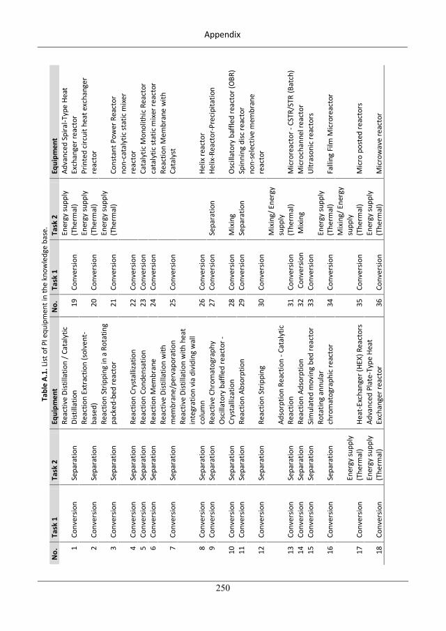
Appendix
250
Tabl
e A.
1. L
ist o
f PI e
quip
men
t in
the
know
ledg
e ba
se.
No.
Ta
sk 1
Ta
sk 2
Eq
uipm
ent
No.
Ta
sk 1
Ta
sk 2
Eq
uipm
ent
1 Co
nver
sion
Sepa
ratio
n Re
activ
e Di
still
atio
n / C
atal
ytic
Di
still
atio
n 19
Co
nver
sion
Ener
gy su
pply
(T
herm
al)
Adva
nced
Spi
ral-T
ype
Heat
Ex
chan
ger r
eact
or
2 Co
nver
sion
Sepa
ratio
n Re
actio
n Ex
trac
tion
(sol
vent
-ba
sed)
20
Co
nver
sion
Ener
gy su
pply
(T
herm
al)
Prin
ted
circ
uit h
eat e
xcha
nger
re
acto
r
3 Co
nver
sion
Sepa
ratio
n Re
actio
n St
rippi
ng in
a R
otat
ing
pack
ed-b
ed re
acto
r 21
Co
nver
sion
Ener
gy su
pply
(T
herm
al)
Cons
tant
Pow
er R
eact
or
4 Co
nver
sion
Sepa
ratio
n Re
actio
n Cr
ysta
lliza
tion
22
Conv
ersio
n
non-
cata
lytic
stat
ic m
ixer
re
acto
r 5
Conv
ersio
n Se
para
tion
Reac
tion
Cond
ensa
tion
23
Conv
ersio
n
Cata
lytic
Mon
olith
ic R
eact
or
6 Co
nver
sion
Sepa
ratio
n Re
actio
n M
embr
ane
24
Conv
ersio
n
cata
lytic
stat
ic m
ixer
reac
tor
7 Co
nver
sion
Sepa
ratio
n Re
activ
e Di
still
atio
n w
ith
mem
bran
e/pe
rvap
orat
ion
25
Conv
ersio
n
Reac
tion
Mem
bran
e w
ith
Cata
lyst
8 Co
nver
sion
Sepa
ratio
n
Reac
tive
Dist
illat
ion
with
hea
t in
tegr
atio
n vi
a di
vidi
ng w
all
colu
mn
26
Conv
ersio
n
Helix
reac
tor
9 Co
nver
sion
Sepa
ratio
n Re
activ
e Ch
rom
atog
raph
y 27
Co
nver
sion
Sepa
ratio
n He
lix-R
eact
or-P
reci
pita
tion
10
Conv
ersio
n Se
para
tion
Osc
illat
ory
baffl
ed re
acto
r -
Crys
talli
zatio
n 28
Co
nver
sion
Mix
ing
Osc
illat
ory
baffl
ed re
acto
r (O
BR)
11
Conv
ersio
n Se
para
tion
Reac
tion
Abso
rptio
n 29
Co
nver
sion
Sepa
ratio
n Sp
inni
ng d
isc re
acto
r
12
Conv
ersio
n Se
para
tion
Reac
tion
Strip
ping
30
Co
nver
sion
no
n-se
lect
ive
mem
bran
e re
acto
r
13
Conv
ersio
n Se
para
tion
Adso
rptio
n Re
actio
n - C
atal
ytic
Re
actio
n 31
Co
nver
sion
Mix
ing/
Ene
rgy
supp
ly
(The
rmal
) M
icro
reac
tor -
CST
R/ST
R (B
atch
) 14
Co
nver
sion
Sepa
ratio
n Re
actio
n Ad
sorp
tion
32
Con
vers
ion
M
ixin
g
Mic
roch
anne
l rea
ctor
15
Co
nver
sion
Sepa
ratio
n Si
mul
ated
mov
ing
bed
reac
tor
33
Conv
ersio
n
Ultr
ason
ic re
acto
rs
16
Conv
ersio
n Se
para
tion
Rota
ting
annu
lar
chro
mat
ogra
phic
reac
tor
34
Conv
ersio
n En
ergy
supp
ly
(The
rmal
) Fa
lling
Film
Mic
rore
acto
r
17
Conv
ersio
n En
ergy
supp
ly
(The
rmal
) He
at-E
xcha
nger
(HEX
) Rea
ctor
s 35
Co
nver
sion
Mix
ing/
Ene
rgy
supp
ly
(The
rmal
) M
icro
pos
ted
reac
tors
18
Conv
ersio
n En
ergy
supp
ly
(The
rmal
) Ad
vanc
ed P
late
-Typ
e He
at
Exch
ange
r rea
ctor
36
Co
nver
sion
Ener
gy su
pply
(T
herm
al)
Mic
row
ave
reac
tor
280
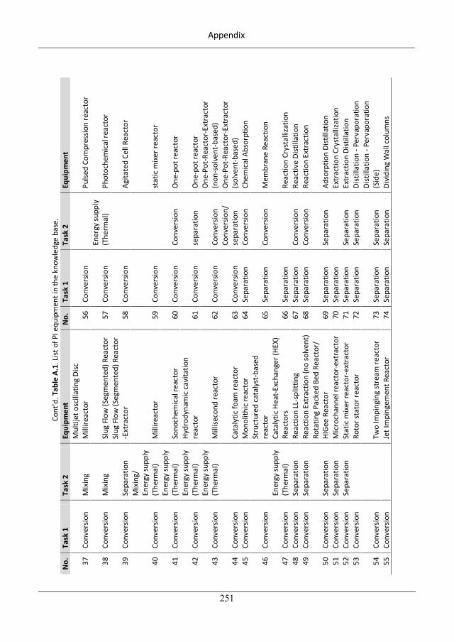
Appendix
251
Co
nt’d
. Tab
le A
.1. L
ist o
f PI e
quip
men
t in
the
know
ledg
e ba
se.
No.
Ta
sk 1
Ta
sk 2
Eq
uipm
ent
No.
Ta
sk 1
Ta
sk 2
Eq
uipm
ent
37
Conv
ersio
n M
ixin
g M
ultij
et o
scill
atin
g Di
sc
Mill
ireac
tor
56
Conv
ersio
n
Pulse
d Co
mpr
essio
n re
acto
r
38
Conv
ersio
n M
ixin
g Sl
ug F
low
(Seg
men
ted)
Rea
ctor
57
Co
nver
sion
Ener
gy su
pply
(T
herm
al)
Phot
oche
mic
al re
acto
r
39
Conv
ersio
n Se
para
tion
Slug
Flo
w (S
egm
ente
d) R
eact
or
-Ext
ract
or
58
Conv
ersio
n
Agita
ted
Cell
Reac
tor
40
Conv
ersio
n
Mix
ing/
En
ergy
supp
ly
(The
rmal
) M
illire
acto
r 59
Co
nver
sion
st
atic
mix
er re
acto
r
41
Conv
ersio
n En
ergy
supp
ly
(The
rmal
) So
noch
emic
al re
acto
r 60
Co
nver
sion
Conv
ersio
n O
ne-p
ot re
acto
r
42
Conv
ersio
n En
ergy
supp
ly
(The
rmal
) Hy
drod
ynam
ic c
avita
tion
reac
tor
61
Conv
ersio
n se
para
tion
One
-pot
reac
tor
43
Conv
ersio
n En
ergy
supp
ly
(The
rmal
) M
illise
cond
reac
tor
62
Conv
ersio
n Co
nver
sion
One
-Pot
-Rea
ctor
-Ext
ract
or
(non
-sol
vent
-bas
ed)
44
Conv
ersio
n
Cata
lytic
foam
reac
tor
63
Conv
ersio
n Co
nver
sion/
se
para
tion
One
-Pot
-Rea
ctor
-Ext
ract
or
(sol
vent
-bas
ed)
45
Conv
ersio
n
Mon
olith
ic re
acto
r 64
Se
para
tion
Conv
ersio
n Ch
emic
al A
bsor
ptio
n
46
Conv
ersio
n
Stru
ctur
ed c
atal
yst-
base
d re
acto
r 65
Se
para
tion
Conv
ersio
n M
embr
ane
Reac
tion
47
Conv
ersio
n En
ergy
supp
ly
(The
rmal
) Ca
taly
tic H
eat-E
xcha
nger
(HEX
) Re
acto
rs
66
Sepa
ratio
n
Re
actio
n Cr
ysta
lliza
tion
48
Conv
ersio
n Se
para
tion
Reac
tion
LL-s
plitt
ing
67
Sepa
ratio
n Co
nver
sion
Reac
tive
Dist
illat
ion
49
Conv
ersio
n Se
para
tion
Reac
tion
Extr
actio
n (n
o so
lven
t)
68
Sepa
ratio
n Co
nver
sion
Reac
tion
Extr
actio
n
50
Conv
ersio
n Se
para
tion
Rota
ting
Pack
ed B
ed R
eact
or/
HIGe
e Re
acto
r 69
Se
para
tion
Sepa
ratio
n Ad
sorp
tion
Dist
illat
ion
51
Conv
ersio
n Se
para
tion
Mic
roch
anne
l rea
ctor
-ext
ract
or
70
Sepa
ratio
n
Extr
actio
n Cr
ysta
lliza
tion
52
Conv
ersio
n Se
para
tion
Stat
ic m
ixer
reac
tor-
extr
acto
r 71
Se
para
tion
Sepa
ratio
n Ex
trac
tion
Dist
illat
ion
53
Conv
ersio
n
Roto
r sta
tor r
eact
or
72
Sepa
ratio
n Se
para
tion
Dist
illat
ion
- Per
vapo
ratio
n
54
Conv
ersio
n
Two
Impi
ngin
g st
ream
reac
tor
73
Sepa
ratio
n Se
para
tion
Dist
illat
ion
- Per
vapo
ratio
n (S
ide)
55
Co
nver
sion
Je
t Im
ping
emen
t Rea
ctor
74
Se
para
tion
Sepa
ratio
n Di
vidi
ng W
all c
olum
ns
281
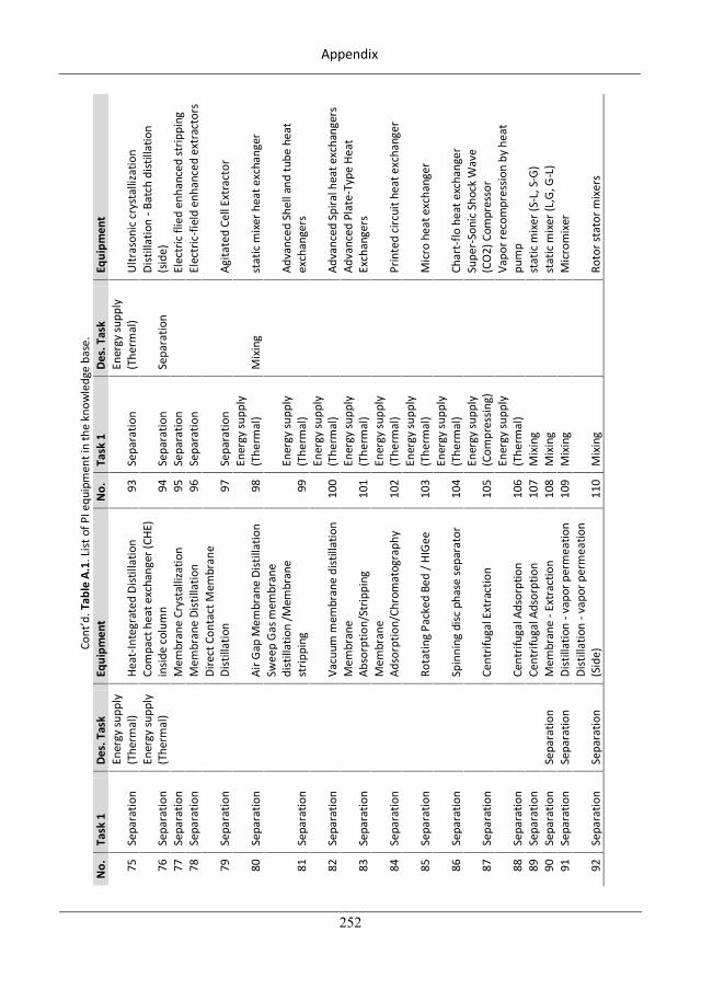
Appendix
252
Co
nt’d
. Tab
le A
.1. L
ist o
f PI e
quip
men
t in
the
know
ledg
e ba
se.
No.
Ta
sk 1
De
s. T
ask
Equi
pmen
t N
o.
Task
1
Des.
Tas
k Eq
uipm
ent
75
Sepa
ratio
n En
ergy
supp
ly
(The
rmal
) He
at-In
tegr
ated
Dist
illat
ion
93
Sepa
ratio
n En
ergy
supp
ly
(The
rmal
) U
ltras
onic
cry
stal
lizat
ion
76
Sepa
ratio
n En
ergy
supp
ly
(The
rmal
) Co
mpa
ct h
eat e
xcha
nger
(CHE
) in
side
colu
mn
94
Sepa
ratio
n Se
para
tion
Dist
illat
ion
- Bat
ch d
istill
atio
n (s
ide)
77
Se
para
tion
M
embr
ane
Crys
talli
zatio
n 95
Se
para
tion
El
ectr
ic fl
ied
enha
nced
strip
ping
78
Se
para
tion
M
embr
ane
Dist
illat
ion
96
Sepa
ratio
n
Elec
tric
-fiel
d en
hanc
ed e
xtra
ctor
s
79
Sepa
ratio
n
Dire
ct C
onta
ct M
embr
ane
Dist
illat
ion
97
Sepa
ratio
n
Agita
ted
Cell
Extr
acto
r
80
Sepa
ratio
n
Air G
ap M
embr
ane
Dist
illat
ion
98
Ener
gy su
pply
(T
herm
al)
Mix
ing
stat
ic m
ixer
hea
t exc
hang
er
81
Sepa
ratio
n
Swee
p G
as m
embr
ane
dist
illat
ion
/Mem
bran
e st
rippi
ng
99
Ener
gy su
pply
(T
herm
al)
Ad
vanc
ed S
hell
and
tube
hea
t ex
chan
gers
82
Sepa
ratio
n
Vacu
um m
embr
ane
dist
illat
ion
100
Ener
gy su
pply
(T
herm
al)
Ad
vanc
ed S
pira
l hea
t exc
hang
ers
83
Sepa
ratio
n
Mem
bran
e Ab
sorp
tion/
Strip
ping
10
1 En
ergy
supp
ly
(The
rmal
)
Adva
nced
Pla
te-T
ype
Heat
Ex
chan
gers
84
Sepa
ratio
n
Mem
bran
e Ad
sorp
tion/
Chro
mat
ogra
phy
102
Ener
gy su
pply
(T
herm
al)
Pr
inte
d ci
rcui
t hea
t exc
hang
er
85
Sepa
ratio
n
Rota
ting
Pack
ed B
ed /
HIG
ee
103
Ener
gy su
pply
(T
herm
al)
M
icro
hea
t exc
hang
er
86
Sepa
ratio
n
Spin
ning
disc
pha
se se
para
tor
104
Ener
gy su
pply
(T
herm
al)
Ch
art-
flo h
eat e
xcha
nger
87
Sepa
ratio
n
Cent
rifug
al E
xtra
ctio
n 10
5 En
ergy
supp
ly
(Com
pres
sing)
Supe
r-So
nic
Shoc
k W
ave
(CO
2) C
ompr
esso
r
88
Sepa
ratio
n
Cent
rifug
al A
dsor
ptio
n 10
6 En
ergy
supp
ly
(The
rmal
)
Vapo
r rec
ompr
essio
n by
hea
t pu
mp
89
Sepa
ratio
n
Cent
rifug
al A
dsor
ptio
n 10
7 M
ixin
g
stat
ic m
ixer
(S-L
, S-G
) 90
Se
para
tion
Sepa
ratio
n M
embr
ane
- Ext
ract
ion
108
Mix
ing
st
atic
mix
er (L
,G, G
-L)
91
Sepa
ratio
n Se
para
tion
Dist
illat
ion
- vap
or p
erm
eatio
n 10
9 M
ixin
g
Mic
rom
ixer
92
Sepa
ratio
n Se
para
tion
Dist
illat
ion
- vap
or p
erm
eatio
n (S
ide)
11
0 M
ixin
g
Roto
r sta
tor m
ixer
s
282
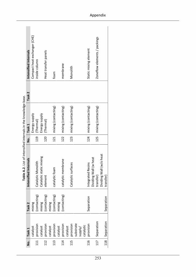
Appendix
253
Ta
ble
A.2.
List
of i
nten
sifie
d in
tern
als i
n th
e kn
owle
dge
base
. N
o.
Task
1
Task
2
Inte
nsifi
ed In
tern
als
No.
Ta
sk 1
Ta
sk 2
In
tens
ified
Inte
rnal
s
111
cata
lyst
pr
ovisi
on
mix
ing
(con
tact
ing)
Ca
taly
tic M
onol
ith
119
Ener
gy su
pply
(T
herm
al)
Co
mpa
ct h
eat e
xcha
nger
(CHE
) in
side
colu
mn
112
cata
lyst
pr
ovisi
on
mix
ing
(con
tact
ing)
Ca
taly
tic st
atic
mix
ing
elem
ent
120
Ener
gy su
pply
(T
herm
al)
He
at tr
ansf
er p
anel
s
113
cata
lyst
pr
ovisi
on
mix
ing
(con
tact
ing)
ca
taly
tic fo
am
121
mix
ing
(con
tact
ing)
foam
114
cata
lyst
pr
ovisi
on
mix
ing
(con
tact
ing)
ca
taly
tic m
embr
ane
122
mix
ing
(con
tact
ing)
mem
bran
e
115
cata
lyst
pr
ovisi
on
Ca
taly
tic su
rfac
es
123
mix
ing
(con
tact
ing)
Mon
olith
116
subs
trat
e su
pply
/ ca
taly
tic
prov
ision
Se
para
tion
Inte
grat
ed R
esin
s 12
4 m
ixin
g (c
onta
ctin
g)
St
atic
mix
ing
elem
ent
117
Sepa
ratio
n
Divi
ding
Wal
l (w
hea
t tr
ansf
er)
125
mix
ing
(con
tact
ing)
Zone
flow
ele
men
ts /
pack
ings
118
Sepa
ratio
n Se
para
tion
Divi
ding
Wal
l (w
/o h
eat
tran
sfer
)
283
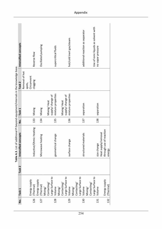
Appendix
254
Tabl
e A.
3. L
ist o
f add
ition
al P
I bey
ond
equi
pmen
t/in
tern
als i
n th
e kn
owle
dge
base
. N
o.
Task
1
Task
2
Inte
nsifi
ed c
once
pts
No.
Ta
sk 1
Ta
sk 2
In
tens
ified
con
cept
s
126
Ener
gy su
pply
(T
herm
al)
In
duct
ive/
Ohm
ic H
eatin
g 13
3 M
ixin
g
Rem
oval
of h
ot
spot
s, Ci
rcum
vent
cl
oggi
ng
Reve
rse
flow
127
Ener
gy su
pply
(T
herm
al)
M
icro
wav
e he
atin
g 13
4 M
ixin
g
Osc
illat
ed p
umpi
ng
128
Mix
ing/
Co
ntac
ting/
La
rge
Surf
ace
to
Volu
me
ge
omet
rical
cha
nge
135
Mix
ing/
Hea
t su
pply
/ cha
nge
of
mix
ture
pro
pert
ies
su
perc
ritic
al fl
uids
129
Mix
ing/
Co
ntac
ting/
La
rge
Surf
ace
to
Volu
me
su
rfac
e ch
ange
13
6
Mix
ing/
Hea
t su
pply
/ cha
nge
of
mix
ture
pro
pert
ies
ho
t/co
ld in
ert g
as/s
team
130
Mix
ing/
Co
ntac
ting/
La
rge
Surf
ace
to
Volu
me
st
ruct
ured
mat
eria
ls 13
7 se
para
tion
ad
ditio
nal r
eact
ion
as se
para
tor
131
Mix
ing/
Co
ntac
ting/
La
rge
Surf
ace
to
Volu
me
siz
e ch
ange
13
8 se
para
tion
U
se o
f ion
ic li
quid
s as s
olve
nt w
ith
no v
apor
pre
ssur
e
132
Ener
gy su
pply
(T
herm
al)
Heat
supp
ly/r
emov
al
thro
ugh
use
of re
actio
n en
ergy
284
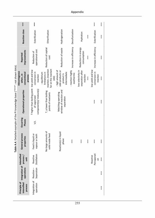
Appendix
255
Tabl
e A.
4. D
etai
led
exam
ple
of th
e PI
kno
wle
dge
base
(“**
*”: n
ot sh
own
data
).
Prin
cipl
e of
in
tens
ified
pr
oces
s
Inte
grat
ion
of
oper
atio
ns
Inte
nsifi
ed
proc
ess /
un
it
Gene
ral p
roce
ss
prop
ertie
s O
ccur
ring
Phas
es
Ope
ratio
nal p
rope
rtie
s
Adva
ntag
eous
w
hen…
in
conv
entio
nal
proc
ess
Repo
rted
im
prov
emen
ts
Reac
tion
clas
s **
*
Inte
grat
ion
of
oper
atio
n Re
actio
n –
Sepa
ratio
n Re
activ
e Di
still
atio
n Fe
ed is
liqu
id o
r va
pour
or b
oth
V/L
T hi
gher
than
boi
ling
poin
t of
vap
orize
d co
mpo
nent
(s)/
mixt
ure(
s)
low
yie
ld a
nd lo
w
conv
ersio
n in
re
actio
n
Redu
ctio
n of
op
erat
iona
l cos
t Es
terif
icat
ion
***
N
o la
rge
amou
nts o
f so
lid in
side
feed
T, p
low
er th
an b
oilin
g po
ints
of r
eact
ants
- equ
ilibr
ium
lim
itatio
ns in
re
actio
n, (r
eact
ion
far o
n th
e re
acta
nt
side)
Redu
ctio
n of
cap
ital
cost
Et
herif
icat
ion
Re
actio
n(s)
in li
quid
ph
ase
M
atch
ing
oper
atin
g w
indo
w o
f rea
ctio
n an
d se
para
tion
- hig
h am
ount
of
side -
prod
ucts
or
prod
uct i
s in
term
edia
te
Redu
ctio
n of
was
te
Hydr
ogen
atio
n
**
*
- r
eact
ion
high
ly
exot
herm
ic
Incr
ease
in e
ffici
ency
De
sulfu
rizat
ion
**
*
lo
w se
lect
ivity
in
sepa
ratio
n af
ter
reac
tion
Redu
ctio
n in
ene
rgy
cons
umpt
ion
Hydr
atio
n
**
*
**
* **
* **
*
Reac
tive
Perv
apor
ati
on
***
**
* lo
w y
ield
and
low
co
nver
sion
in
reac
tion
Incr
ease
in e
ffici
ency
Es
terif
icat
ion
***
***
***
***
***
**
* **
* **
* **
* **
*
285
Appendix
256
A.2. List of phenomena in the phenomena library of the knowledge base
The knowledge base contains currently a number of 49 phenomena usable for the phenomena based
workflow for the generation/synthesis of novel process options. The 49 phenomena are presented in
Table A.5 listed by their class (see section 2.2.2). Besides the description, also the information on
whether or not a general mathematical model is stored on the library is given. Besides this information,
also the important pure component properties for the identification of these phenomena to fulfill a task
under investigation as well as information about the operating window of each phenomenon are stored
in the knowledge base (but not shown here).
286
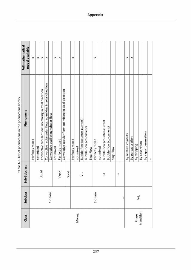
Appendix
257
Tabl
e A.
5. L
ist o
f phe
nom
ena
in th
e ph
enom
ena
libra
ry.
Clas
s Su
bcla
ss
Sub-
Subc
lass
Ph
enom
ena
Full
mat
hem
atic
al
mod
el a
vaila
ble
Mix
ing
1-ph
ase
Liqu
id
Perf
ectly
mix
ed
x no
t mix
ed
x Co
nvec
tive
tubu
lar f
low
: no
mix
ing
in a
xial
dire
ctio
n x
Conv
ectiv
e re
ctan
gula
r flo
w: n
o m
ixin
g in
axi
al d
irect
ion
x Co
nvec
tive
osci
llatin
g tu
bula
r flo
w
Vapo
r no
t mix
ed
x Pe
rfec
tly m
ixed
x
Conv
ectiv
e tu
bula
r flo
w: n
o m
ixin
g in
axi
al d
irect
ion
So
lid
…
2-ph
ase
V-L
Perf
ectly
mix
ed
x no
t mix
ed
Bu
bble
-flow
(cou
nter
-cur
rent
)
Bubb
le-fl
ow (c
o-cu
rren
t)
Slug
-Flo
w
L-L
Perf
ectly
mix
ed
x no
t mix
ed
Bu
bble
-flow
(cou
nter
-cur
rent
Bubb
le-fl
ow (c
o-cu
rren
t)
Slug
-Flo
w
…
…
Phas
e tr
ansit
ion
V-L
by re
lativ
e vo
latil
ity
x by
per
vapo
ratio
n x
by st
rippi
ng
by
abs
orpt
ion
by
vap
or p
erm
eatio
n
…
287
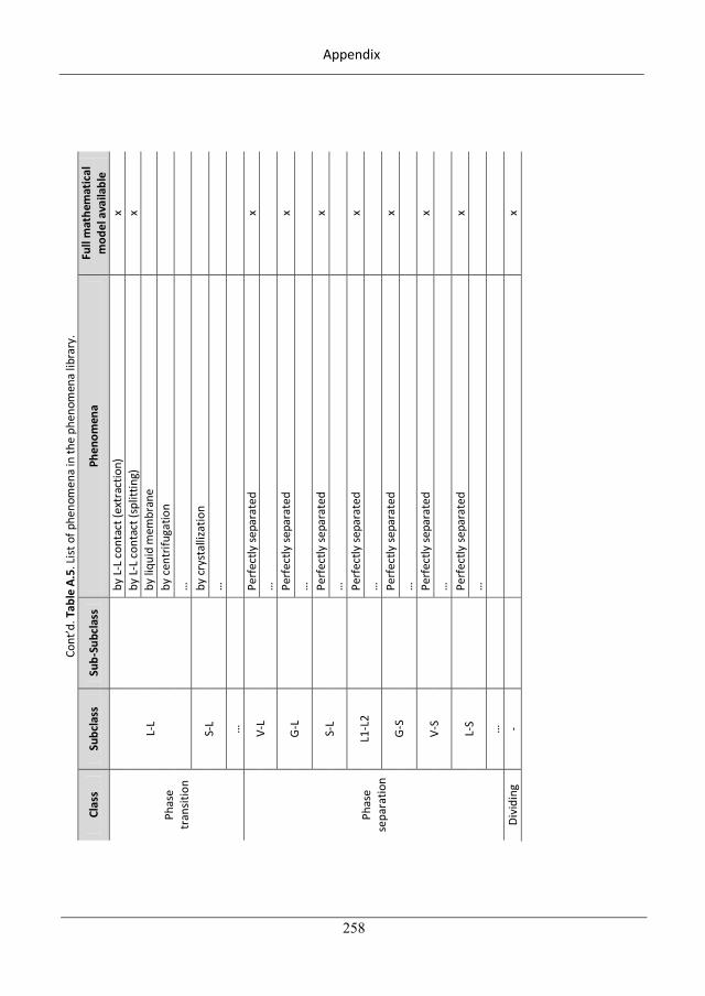
Appendix
258
Cont
’d. T
able
A.5
. List
of p
heno
men
a in
the
phen
omen
a lib
rary
.
Clas
s Su
bcla
ss
Sub-
Subc
lass
Ph
enom
ena
Full
mat
hem
atic
al
mod
el a
vaila
ble
Phas
e tr
ansit
ion
L-L
by L
-L c
onta
ct (e
xtra
ctio
n)
x by
L-L
con
tact
(spl
ittin
g)
x by
liqu
id m
embr
ane
by
cen
trifu
gatio
n
…
S-L
by
cry
stal
lizat
ion
…
…
Phas
e se
para
tion
V-L
Pe
rfec
tly se
para
ted
x …
G-L
Perf
ectly
sepa
rate
d x
…
S-L
Pe
rfec
tly se
para
ted
x …
L1-L
2
Perf
ectly
sepa
rate
d x
…
G-S
Perf
ectly
sepa
rate
d x
…
V-S
Pe
rfec
tly se
para
ted
x …
L-S
Pe
rfec
tly se
para
ted
x …
…
Di
vidi
ng
-
x
288
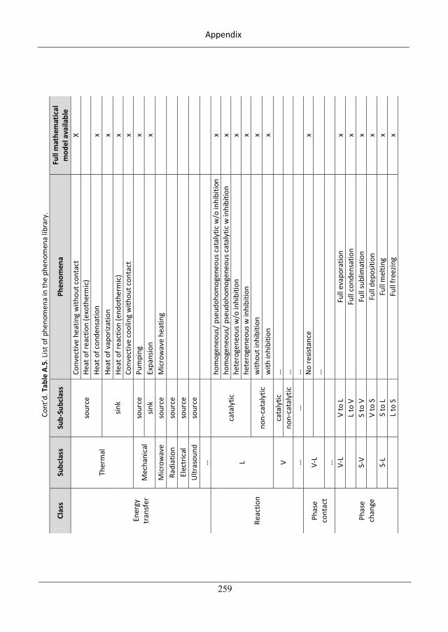
Appendix
259
Cont
’d. T
able
A.5
. List
of p
heno
men
a in
the
phen
omen
a lib
rary
.
Clas
s Su
bcla
ss
Sub-
Subc
lass
Ph
enom
ena
Full
mat
hem
atic
al
mod
el a
vaila
ble
Ener
gy
tran
sfer
Ther
mal
sour
ce
Conv
ectiv
e he
atin
g w
ithou
t con
tact
X
Heat
of r
eact
ion
(exo
ther
mic
)
Heat
of c
onde
nsat
ion
x
sink
Heat
of v
apor
izatio
n x
Heat
of r
eact
ion
(end
othe
rmic
) x
Conv
ectiv
e co
olin
g w
ithou
t con
tact
x
Mec
hani
cal
sour
ce
Pum
ping
x
sink
Expa
nsio
n x
Mic
row
ave
sour
ce
Mic
row
ave
heat
ing
Ra
diat
ion
sour
ce
Elec
tric
al
sour
ce
Ultr
asou
nd
sour
ce
…
Reac
tion
L ca
taly
tic
hom
ogen
eous
/ pse
udoh
omog
eneo
us c
atal
ytic
w/o
inhi
bitio
n x
hom
ogen
eous
/ pse
udoh
omog
eneo
us c
atal
ytic
w in
hibi
tion
x he
tero
gene
ous w
/o in
hibi
tion
x he
tero
gene
ous w
inhi
bitio
n x
non-
cata
lytic
w
ithou
t inh
ibiti
on
x w
ith in
hibi
tion
x
V ca
taly
tic
…
no
n-ca
taly
tic
…
…
…
…
Phas
e co
ntac
t V-
L
No
resis
tanc
e x
…
…
Phas
e ch
ange
V-L
V to
L
Full
evap
orat
ion
x
L to
V
Full
cond
ensa
tion
x S-
V S
to V
Fu
ll su
blim
atio
n x
V
to S
Fu
ll de
posit
ion
x S-
L S
to L
Full
mel
ting
x
L to
S
Full
free
zing
x
289
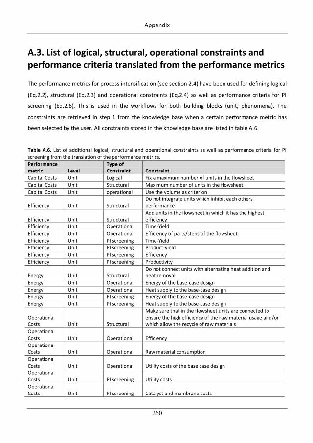
Appendix
260
A.3. List of logical, structural, operational constraints and performance criteria translated from the performance metrics
The performance metrics for process intensification (see section 2.4) have been used for defining logical
(Eq.2.2), structural (Eq.2.3) and operational constraints (Eq.2.4) as well as performance criteria for PI
screening (Eq.2.6). This is used in the workflows for both building blocks (unit, phenomena). The
constraints are retrieved in step 1 from the knowledge base when a certain performance metric has
been selected by the user. All constraints stored in the knowledge base are listed in table A.6.
Table A.6. List of additional logical, structural and operational constraints as well as performance criteria for PI screening from the translation of the performance metrics. Performance metric Level
Type of Constraint Constraint
Capital Costs Unit Logical Fix a maximum number of units in the flowsheet Capital Costs Unit Structural Maximum number of units in the flowsheet Capital Costs Unit operational Use the volume as criterion
Efficiency Unit Structural Do not integrate units which inhibit each others performance
Efficiency Unit Structural Add units in the flowsheet in which it has the highest efficiency
Efficiency Unit Operational Time-Yield Efficiency Unit Operational Efficiency of parts/steps of the flowsheet Efficiency Unit PI screening Time-Yield Efficiency Unit PI screening Product-yield Efficiency Unit PI screening Efficiency Efficiency Unit PI screening Productivity
Energy Unit Structural Do not connect units with alternating heat addition and heat removal
Energy Unit Operational Energy of the base-case design Energy Unit Operational Heat supply to the base-case design Energy Unit PI screening Energy of the base-case design Energy Unit PI screening Heat supply to the base-case design
Operational Costs Unit Structural
Make sure that in the flowsheet units are connected to ensure the high efficiency of the raw material usage and/or which allow the recycle of raw materials
Operational Costs Unit Operational Efficiency Operational Costs Unit Operational Raw material consumption Operational Costs Unit Operational Utility costs of the base case design Operational Costs Unit PI screening Utility costs Operational Costs Unit PI screening Catalyst and membrane costs
290
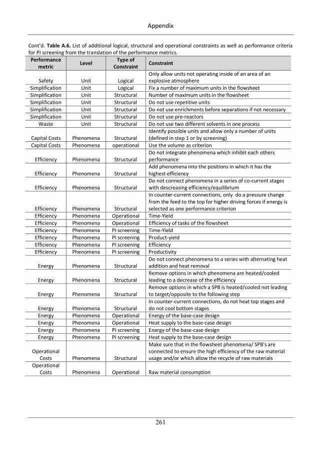
Appendix
261
Cont’d. Table A.6. List of additional logical, structural and operational constraints as well as performance criteria for PI screening from the translation of the performance metrics. Performance
metric Level Type of Constraint Constraint
Safety Unit Logical Only allow units not operating inside of an area of an explosive atmosphere
Simplification Unit Logical Fix a number of maximum units in the flowsheet Simplification Unit Structural Number of maximum units in the flowsheet Simplification Unit Structural Do not use repetitive units Simplification Unit Structural Do not use enrichments before separations if not necessary Simplification Unit Structural Do not use pre-reactors
Waste Unit Structural Do not use two different solvents in one process
Capital Costs Phenomena Structural Identify possible units and allow only a number of units (defined in step 1 or by screening)
Capital Costs Phenomena operational Use the volume as criterion
Efficiency Phenomena Structural Do not integrate phenomena which inhibit each others performance
Efficiency Phenomena Structural Add phenomena into the positions in which it has the highest efficiency
Efficiency Phenomena Structural Do not connect phenomena in a series of co-current stages with descreasing efficiency/equilibrium
Efficiency Phenomena Structural
In counter-current connections, only do a pressure change from the feed to the top for higher driving forces if energy is selected as one performance criterion
Efficiency Phenomena Operational Time-Yield Efficiency Phenomena Operational Efficiency of tasks of the flowsheet Efficiency Phenomena PI screening Time-Yield Efficiency Phenomena PI screening Product-yield Efficiency Phenomena PI screening Efficiency Efficiency Phenomena PI screening Productivity
Energy Phenomena Structural Do not connect phenomena to a series with alternating heat addition and heat removal
Energy Phenomena Structural Remove options in which phenomena are heated/cooled leading to a decrease of the efficiency
Energy Phenomena Structural Remove options in which a SPB is heated/cooled not leading to target/opposite to the following step
Energy Phenomena Structural In counter-current connections, do not heat top stages and do not cool bottom stages
Energy Phenomena Operational Energy of the base-case design Energy Phenomena Operational Heat supply to the base-case design Energy Phenomena PI screening Energy of the base-case design Energy Phenomena PI screening Heat supply to the base-case design
Operational Costs Phenomena Structural
Make sure that in the flowsheet phenomena/ SPB's are connected to ensure the high efficiency of the raw material usage and/or which allow the recycle of raw materials
Operational Costs Phenomena Operational Raw material consumption
291
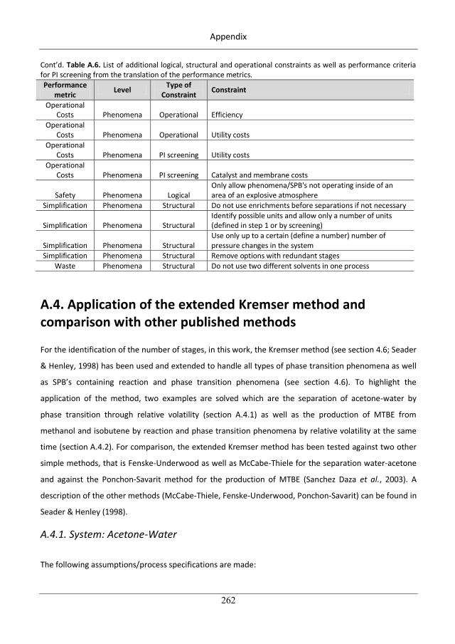
Appendix
262
Cont’d. Table A.6. List of additional logical, structural and operational constraints as well as performance criteria for PI screening from the translation of the performance metrics. Performance
metric Level Type of Constraint Constraint
Operational Costs Phenomena Operational Efficiency
Operational Costs Phenomena Operational Utility costs
Operational Costs Phenomena PI screening Utility costs
Operational Costs Phenomena PI screening Catalyst and membrane costs
Safety Phenomena Logical Only allow phenomena/SPB's not operating inside of an area of an explosive atmosphere
Simplification Phenomena Structural Do not use enrichments before separations if not necessary
Simplification Phenomena Structural Identify possible units and allow only a number of units (defined in step 1 or by screening)
Simplification Phenomena Structural Use only up to a certain (define a number) number of pressure changes in the system
Simplification Phenomena Structural Remove options with redundant stages Waste Phenomena Structural Do not use two different solvents in one process
A.4. Application of the extended Kremser method and comparison with other published methods
For the identification of the number of stages, in this work, the Kremser method (see section 4.6; Seader
& Henley, 1998) has been used and extended to handle all types of phase transition phenomena as well
as SPB’s containing reaction and phase transition phenomena (see section 4.6). To highlight the
application of the method, two examples are solved which are the separation of acetone-water by
phase transition through relative volatility (section A.4.1) as well as the production of MTBE from
methanol and isobutene by reaction and phase transition phenomena by relative volatility at the same
time (section A.4.2). For comparison, the extended Kremser method has been tested against two other
simple methods, that is Fenske-Underwood as well as McCabe-Thiele for the separation water-acetone
and against the Ponchon-Savarit method for the production of MTBE (Sanchez Daza et al., 2003). A
description of the other methods (McCabe-Thiele, Fenske-Underwood, Ponchon-Savarit) can be found in
Seader & Henley (1998).
A.4.1. System: Acetone-Water
The following assumptions/process specifications are made:
292
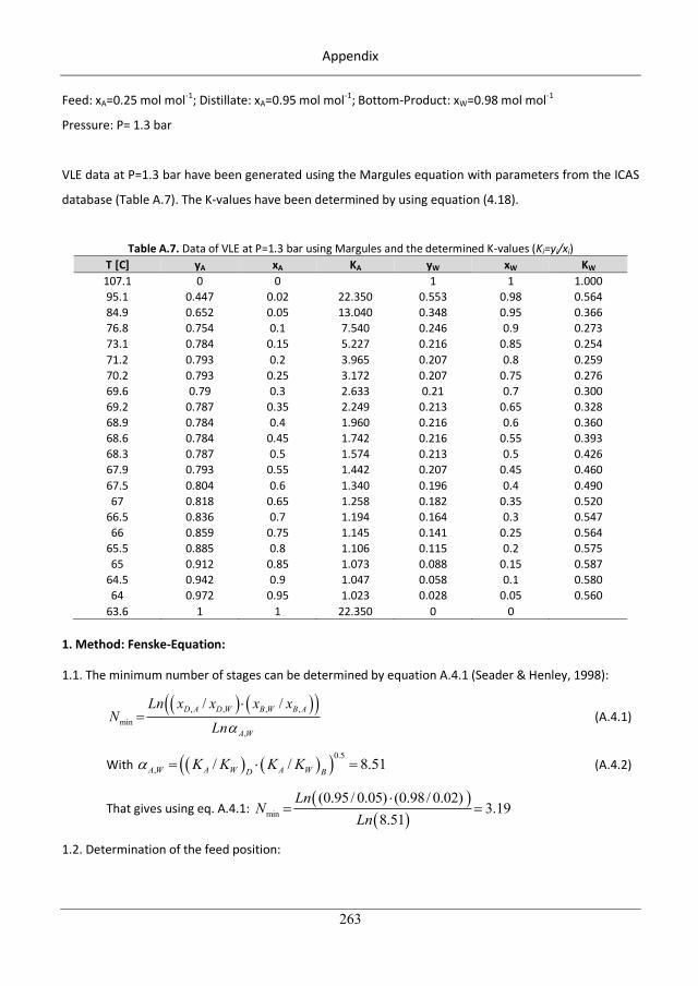
Appendix
263
Feed: xA=0.25 mol mol-1; Distillate: xA=0.95 mol mol-1; Bottom-Product: xW=0.98 mol mol-1
Pressure: P= 1.3 bar
VLE data at P=1.3 bar have been generated using the Margules equation with parameters from the ICAS
database (Table A.7). The K-values have been determined by using equation (4.18).
Table A.7. Data of VLE at P=1.3 bar using Margules and the determined K-values (Ki=yi/xi) T [C] yA xA KA yW xW KW 107.1 0 0 1 1 1.000 95.1 0.447 0.02 22.350 0.553 0.98 0.564 84.9 0.652 0.05 13.040 0.348 0.95 0.366 76.8 0.754 0.1 7.540 0.246 0.9 0.273 73.1 0.784 0.15 5.227 0.216 0.85 0.254 71.2 0.793 0.2 3.965 0.207 0.8 0.259 70.2 0.793 0.25 3.172 0.207 0.75 0.276 69.6 0.79 0.3 2.633 0.21 0.7 0.300 69.2 0.787 0.35 2.249 0.213 0.65 0.328 68.9 0.784 0.4 1.960 0.216 0.6 0.360 68.6 0.784 0.45 1.742 0.216 0.55 0.393 68.3 0.787 0.5 1.574 0.213 0.5 0.426 67.9 0.793 0.55 1.442 0.207 0.45 0.460 67.5 0.804 0.6 1.340 0.196 0.4 0.490 67 0.818 0.65 1.258 0.182 0.35 0.520
66.5 0.836 0.7 1.194 0.164 0.3 0.547 66 0.859 0.75 1.145 0.141 0.25 0.564
65.5 0.885 0.8 1.106 0.115 0.2 0.575 65 0.912 0.85 1.073 0.088 0.15 0.587
64.5 0.942 0.9 1.047 0.058 0.1 0.580 64 0.972 0.95 1.023 0.028 0.05 0.560
63.6 1 1 22.350 0 0 1. Method: Fenske-Equation:
1.1. The minimum number of stages can be determined by equation A.4.1 (Seader & Henley, 1998):
, , , ,min
,
/ /D A D W B W B A
A W
Ln x x x xN
Ln (A.4.1)
With 0.5
, / / 8.51A W A W A WD BK K K K (A.4.2)
That gives using eq. A.4.1: min
(0.95/ 0.05) (0.98/ 0.02)3.19
8.51Ln
NLn
1.2. Determination of the feed position:
293
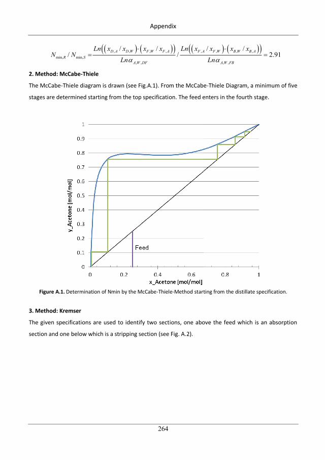
Appendix
264
, , , , , , , ,min, min,
, , , ,
/ / / // / 2.91D A D W F W F A F A F W B W B A
R SA W DF A W FB
Ln x x x x Ln x x x xN N
Ln Ln
2. Method: McCabe-Thiele
The McCabe-Thiele diagram is drawn (see Fig.A.1). From the McCabe-Thiele Diagram, a minimum of five
stages are determined starting from the top specification. The feed enters in the fourth stage.
Figure A.1. Determination of Nmin by the McCabe-Thiele-Method starting from the distillate specification.
3. Method: Kremser
The given specifications are used to identify two sections, one above the feed which is an absorption
section and one below which is a stripping section (see Fig. A.2).
294
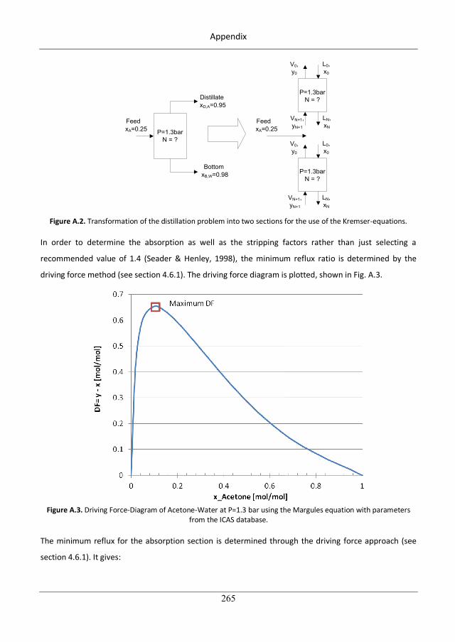
Appendix
265
P=1.3barN = ?
FeedxA=0.25
DistillatexD,A=0.95
BottomxB,W=0.98
L0,x0
LN,xN
VN+1,yN+1
V0,y0
L0,x0
LN,xN
VN+1,yN+1
V0,y0
FeedxA=0.25
P=1.3barN = ?
P=1.3barN = ?
Figure A.2. Transformation of the distillation problem into two sections for the use of the Kremser-equations.
In order to determine the absorption as well as the stripping factors rather than just selecting a
recommended value of 1.4 (Seader & Henley, 1998), the minimum reflux ratio is determined by the
driving force method (see section 4.6.1). The driving force diagram is plotted, shown in Fig. A.3.
Figure A.3. Driving Force-Diagram of Acetone-Water at P=1.3 bar using the Margules equation with parameters
from the ICAS database.
The minimum reflux for the absorption section is determined through the driving force approach (see
section 4.6.1). It gives:
295
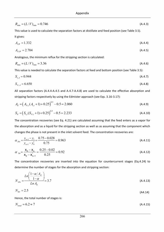
Appendix
266
min min( / ) 0.746R L V (A.4.3)
This value is used to calculate the separation factors at distillate and feed position (see Table 3.5). It gives:
1, 1.332WA (A.4.4)
, 2.704N WA (A.4.5)
Analogous, the minimum reflux for the stripping section is calculated:
min min( / ) 3.36R L V (A.4.6)
This value is needed to calculate the separation factors at feed and bottom position (see Table 3.5):
1, 0.944AS (A.4.7)
, 6.650N AS (A.4.8)
All separation factors (A.4.4-A.4.5 and A.4.7-A.4.8) are used to calculate the effective absorption and
stripping factors respectively by using the Edmister approach (see Eqs. 3.16-3.17): 0.5
, 1,( 1) 0.25 0.5 2.060E N i iA A A (A.4.9)
0.51, ,( 1) 0.25 0.5 2.233E i N iS S S
(A.4.10)
The concentration recoveries (see Eq. 4.21) are calculated assuming that the feed enters as a vapor for
the absorption and as a liquid for the stripping section as well as as assuming that the component which
changes the phase is not present in the inlet solvent feed. The concentration recoveries are:
1 1
1 0
0.75 0.028 0.9630.75
nAbs
n
y yy y
(A.4.11)
0.25 0.02 0.920.25Str
0 n*
0 n 1
x xx x
(A.4.12)
The concentration recoveries are inserted into the equation for countercurrent stages (Eq.4.24) to
determine the number of stages for the absorption and stripping section:
11 3.7
E
AbsE
ALnN
Ln A (A.4.13)
2.5StrN (A4.14)
Hence, the total number of stages is:
6.2 7totalN (A.4.15)
296
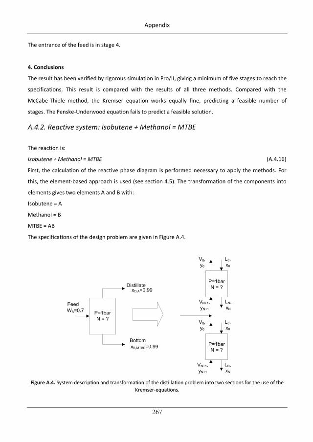
Appendix
267
The entrance of the feed is in stage 4.
4. Conclusions
The result has been verified by rigorous simulation in Pro/II, giving a minimum of five stages to reach the
specifications. This result is compared with the results of all three methods. Compared with the
McCabe-Thiele method, the Kremser equation works equally fine, predicting a feasible number of
stages. The Fenske-Underwood equation fails to predict a feasible solution.
A.4.2. Reactive system: Isobutene + Methanol = MTBE
The reaction is:
Isobutene + Methanol = MTBE (A.4.16)
First, the calculation of the reactive phase diagram is performed necessary to apply the methods. For
this, the element-based approach is used (see section 4.5). The transformation of the components into
elements gives two elements A and B with:
Isobutene = A
Methanol = B
MTBE = AB
The specifications of the design problem are given in Figure A.4.
P=1barN = ?
FeedWA=0.7
DistillatexD,A=0.99
BottomxB,MTBE=0.99
L0,x0
LN,xN
VN+1,yN+1
V0,y0
L0,x0
LN,xN
VN+1,yN+1
V0,y0
P=1barN = ?
P=1barN = ?
Figure A.4. System description and transformation of the distillation problem into two sections for the use of the
Kremser-equations.
297
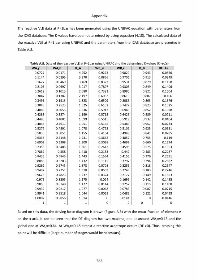
Appendix
268
The reactive VLE data at P=1bar has been generated using the UNIFAC equation with parameters from
the ICAS database. The K-values have been determined by using equation (4.18). The calculated data of
the reactive VLE at P=1 bar using UNIFAC and the parameters from the ICAS database are presented in
Table A.8.
Table A.8. Data of the reactive VLE at P=1bar using UNIFAC and the determined K-values (Ki=yi/xi) WA,y WA,x K_A WB_y WB,x K_B DF (A)
0.0727 0.0171 4.252 0.9273 0.9829 0.943 0.0556 0.1144 0.0295 3.878 0.8856 0.9705 0.913 0.0849 0.1627 0.0469 3.469 0.8373 0.9531 0.879 0.1158 0.2103 0.0697 3.017 0.7897 0.9303 0.849 0.1406 0.2619 0.1015 2.580 0.7381 0.8985 0.821 0.1604 0.3047 0.1387 2.197 0.6953 0.8613 0.807 0.166 0.3491 0.1915 1.823 0.6509 0.8085 0.805 0.1576 0.3848 0.2523 1.525 0.6152 0.7477 0.823 0.1325 0.4083 0.3055 1.336 0.5917 0.6945 0.852 0.1028 0.4285 0.3574 1.199 0.5715 0.6426 0.889 0.0711 0.4485 0.4081 1.099 0.5515 0.5919 0.932 0.0404 0.4845 0.4611 1.051 0.5155 0.5389 0.957 0.0234 0.5272 0.4891 1.078 0.4728 0.5109 0.925 0.0381 0.5836 0.5051 1.155 0.4164 0.4949 0.841 0.0785 0.6338 0.5148 1.231 0.3662 0.4852 0.755 0.119 0.6902 0.5308 1.300 0.3098 0.4692 0.660 0.1594 0.7358 0.5405 1.361 0.2642 0.4595 0.575 0.1953 0.7867 0.558 1.410 0.2133 0.442 0.483 0.2287 0.8436 0.5845 1.443 0.1564 0.4155 0.376 0.2591 0.8885 0.6203 1.432 0.1115 0.3797 0.294 0.2682 0.9292 0.6745 1.378 0.0708 0.3255 0.218 0.2547 0.9497 0.7251 1.310 0.0503 0.2749 0.183 0.2246 0.9676 0.7823 1.237 0.0324 0.2177 0.149 0.1853
0.976 0.8305 1.175 0.024 0.1695 0.142 0.1455 0.9856 0.8748 1.127 0.0144 0.1252 0.115 0.1108 0.9932 0.9217 1.077 0.0068 0.0783 0.087 0.0715 0.9941 0.9518 1.044 0.0059 0.0482 0.122 0.0423 1.0002 0.9856 1.014 0 0.0144 0 0.0146
1 1 1 0 0 0 0
Based on this data, the driving force diagram is drawn (Figure A.5) with the moar fraction of element A
on the x-axis. It can be seen that the DF diagram has two maxima, one at around WA,x=0.13 and the
global one at WA,x=0.64. At WA,x=0.48 almost a reactive azeotrope occurs (DF->0). Thus, crossing this
point will be difficult (large number of stages would be necessary).
298
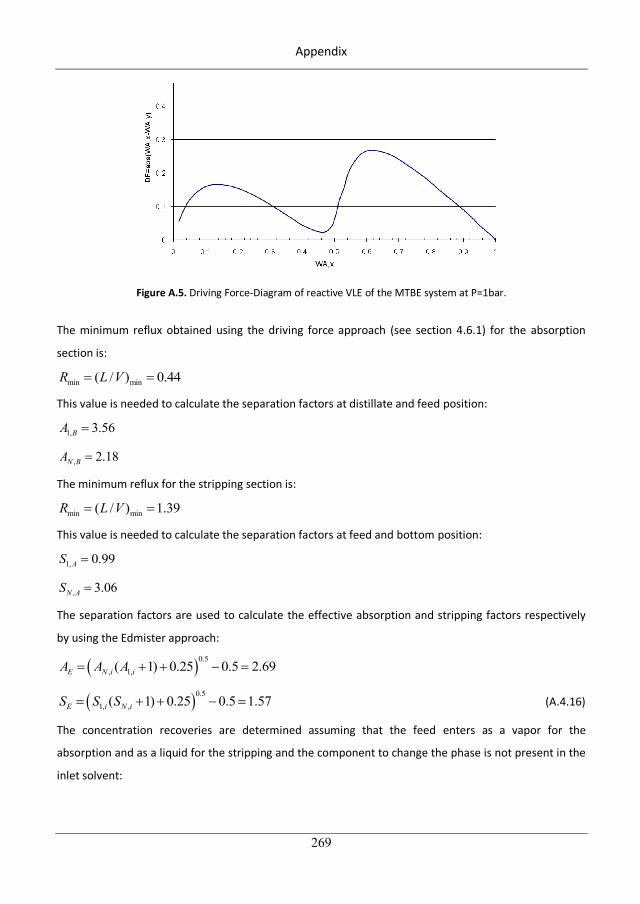
Appendix
269
Figure A.5. Driving Force-Diagram of reactive VLE of the MTBE system at P=1bar.
The minimum reflux obtained using the driving force approach (see section 4.6.1) for the absorption
section is:
min min( / ) 0.44R L V
This value is needed to calculate the separation factors at distillate and feed position:
1, 3.56BA
, 2.18N BA The minimum reflux for the stripping section is:
min min( / ) 1.39R L V
This value is needed to calculate the separation factors at feed and bottom position:
1, 0.99AS
, 3.06N AS
The separation factors are used to calculate the effective absorption and stripping factors respectively
by using the Edmister approach: 0.5
, 1,( 1) 0.25 0.5 2.69E N i iA A A
0.51, ,( 1) 0.25 0.5 1.57E i N iS S S (A.4.16)
The concentration recoveries are determined assuming that the feed enters as a vapor for the
absorption and as a liquid for the stripping and the component to change the phase is not present in the
inlet solvent:
299
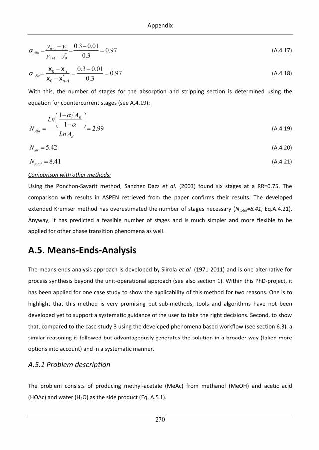
Appendix
270
1 1
1 0
0.3 0.01 0.970.3
nAbs
n
y yy y
(A.4.17)
0.3 0.01 0.970.3Str
0 n*
0 n 1
x xx x
(A.4.18)
With this, the number of stages for the absorption and stripping section is determined using the
equation for countercurrent stages (see A.4.19):
11 2.99
E
AbsE
ALnN
Ln A (A.4.19)
5.42StrN (A.4.20)
8.41totalN (A.4.21)
Comparison with other methods:
Using the Ponchon-Savarit method, Sanchez Daza et al. (2003) found six stages at a RR=0.75. The
comparison with results in ASPEN retrieved from the paper confirms their results. The developed
extended Kremser method has overestimated the number of stages necessary (Ntotal=8.41, Eq.A.4.21).
Anyway, it has predicted a feasible number of stages and is much simpler and more flexible to be
applied for other phase transition phenomena as well.
A.5. Means-Ends-Analysis
The means-ends analysis approach is developed by Siirola et al. (1971-2011) and is one alternative for
process synthesis beyond the unit-operational approach (see also section 1). Within this PhD-project, it
has been applied for one case study to show the applicability of this method for two reasons. One is to
highlight that this method is very promising but sub-methods, tools and algorithms have not been
developed yet to support a systematic guidance of the user to take the right decisions. Second, to show
that, compared to the case study 3 using the developed phenomena based workflow (see section 6.3), a
similar reasoning is followed but advantageously generates the solution in a broader way (taken more
options into account) and in a systematic manner.
A.5.1 Problem description
The problem consists of producing methyl-acetate (MeAc) from methanol (MeOH) and acetic acid
(HOAc) and water (H2O) as the side product (Eq. A.5.1).
300
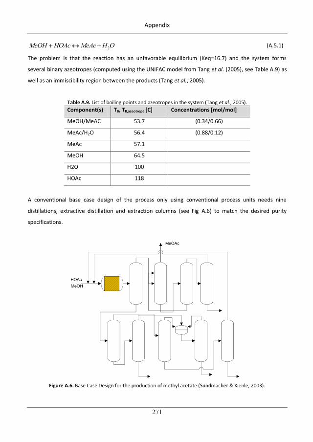
Appendix
271
2MeOH HOAc MeAc H O (A.5.1)
The problem is that the reaction has an unfavorable equilibrium (Keq=16.7) and the system forms
several binary azeotropes (computed using the UNIFAC model from Tang et al. (2005), see Table A.9) as
well as an immiscibility region between the products (Tang et al., 2005).
Table A.9. List of boiling points and azeotropes in the system (Tang et al., 2005). Component(s) TB, TB,azeotrope [C] Concentrations [mol/mol]
MeOH/MeAC 53.7 (0.34/0.66)
MeAc/H2O 56.4 (0.88/0.12)
MeAc 57.1
MeOH 64.5
H2O 100
HOAc 118
A conventional base case design of the process only using conventional process units needs nine
distillations, extractive distillation and extraction columns (see Fig A.6) to match the desired purity
specifications.
Figure A.6. Base Case Design for the production of methyl acetate (Sundmacher & Kienle, 2003).
301
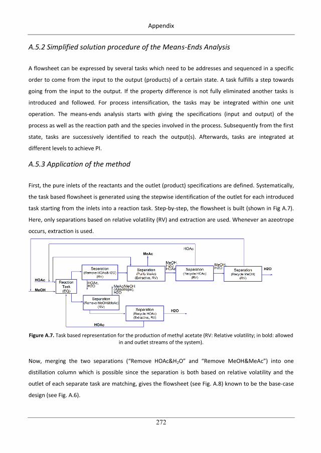
Appendix
272
A.5.2 Simplified solution procedure of the Means-Ends Analysis
A flowsheet can be expressed by several tasks which need to be addresses and sequenced in a specific
order to come from the input to the output (products) of a certain state. A task fulfills a step towards
going from the input to the output. If the property difference is not fully eliminated another tasks is
introduced and followed. For process intensification, the tasks may be integrated within one unit
operation. The means-ends analysis starts with giving the specifications (input and output) of the
process as well as the reaction path and the species involved in the process. Subsequently from the first
state, tasks are successively identified to reach the output(s). Afterwards, tasks are integrated at
different levels to achieve PI.
A.5.3 Application of the method
First, the pure inlets of the reactants and the outlet (product) specifications are defined. Systematically,
the task based flowsheet is generated using the stepwise identification of the outlet for each introduced
task starting from the inlets into a reaction task. Step-by-step, the flowsheet is built (shown in Fig A.7).
Here, only separations based on relative volatility (RV) and extraction are used. Whenever an azeotrope
occurs, extraction is used.
Figure A.7. Task based representation for the production of methyl acetate (RV: Relative volatility; in bold: allowed
in and outlet streams of the system).
Now, merging the two separations (“Remove HOAc&H2O” and “Remove MeOH&MeAc”) into one
distillation column which is possible since the separation is both based on relative volatility and the
outlet of each separate task are matching, gives the flowsheet (see Fig. A.8) known to be the base-case
design (see Fig. A.6).
302
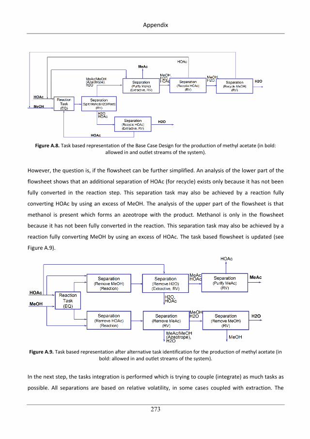
Appendix
273
Figure A.8. Task based representation of the Base Case Design for the production of methyl acetate (in bold:
allowed in and outlet streams of the system).
However, the question is, if the flowsheet can be further simplified. An analysis of the lower part of the
flowsheet shows that an additional separation of HOAc (for recycle) exists only because it has not been
fully converted in the reaction step. This separation task may also be achieved by a reaction fully
converting HOAc by using an excess of MeOH. The analysis of the upper part of the flowsheet is that
methanol is present which forms an azeotrope with the product. Methanol is only in the flowsheet
because it has not been fully converted in the reaction. This separation task may also be achieved by a
reaction fully converting MeOH by using an excess of HOAc. The task based flowsheet is updated (see
Figure A.9).
Figure A.9. Task based representation after alternative task identification for the production of methyl acetate (in
bold: allowed in and outlet streams of the system).
In the next step, the tasks integration is performed which is trying to couple (integrate) as much tasks as
possible. All separations are based on relative volatility, in some cases coupled with extraction. The
303
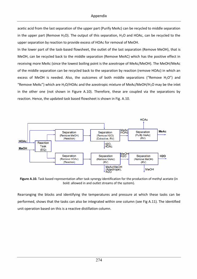
Appendix
274
acetic acid from the last separation of the upper part (Purify MeAc) can be recycled to middle separation
in the upper part (Remove H2O). The output of this separation, H2O and HOAc, can be recycled to the
upper separation by reaction to provide excess of HOAc for removal of MeOH.
In the lower part of the task-based flowsheet, the outlet of the last separation (Remove MeOH), that is
MeOH, can be recycled back to the middle separation (Remove MeAC) which has the positive effect in
receiving more MeAc (since the lowest boiling point is the azeotrope of MeAc/MeOH). The MeOH/MeAc
of the middle separation can be recycled back to the separation by reaction (remove HOAc) in which an
excess of MeOH is needed. Also, the outcomes of both middle separations (“Remove H2O”) and
“Remove MeAc”) which are H2O/HOAc and the azeotropic mixture of MeAc/MeOH/H2O may be the inlet
in the other one (not shown in Figure A.10). Therefore, these are coupled via the separations by
reaction. Hence, the updated task based flowsheet is shown in Fig. A.10.
Figure A.10. Task based representation after task synergy identification for the production of methyl acetate (in
bold: allowed in and outlet streams of the system).
Rearranging the blocks and identifying the temperatures and pressure at which these tasks can be
performed, shows that the tasks can also be integrated within one column (see Fig A.11). The identified
unit operation based on this is a reactive distillation column.
304
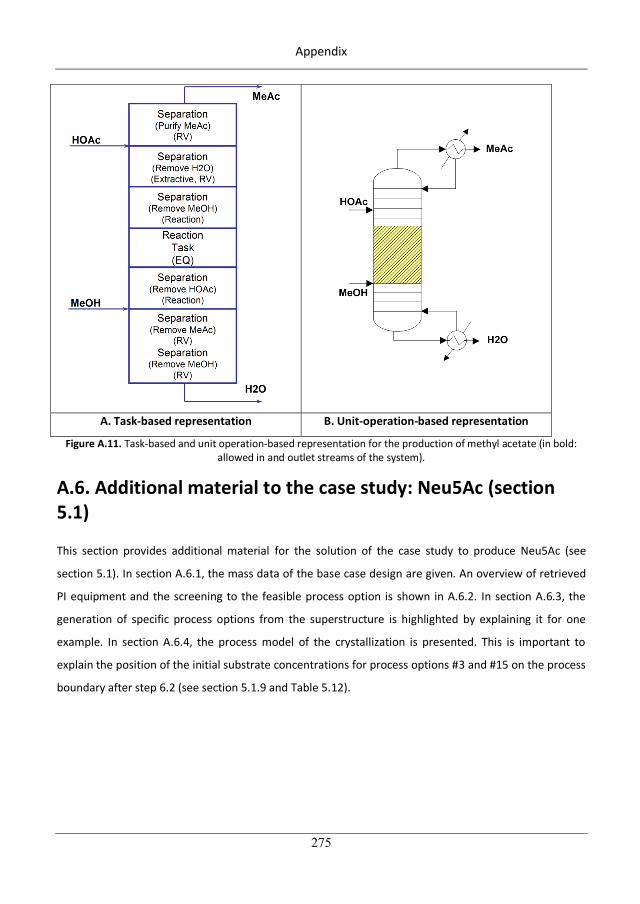
Appendix
275
A. Task-based representation B. Unit-operation-based representation
Figure A.11. Task-based and unit operation-based representation for the production of methyl acetate (in bold: allowed in and outlet streams of the system).
A.6. Additional material to the case study: Neu5Ac (section 5.1)
This section provides additional material for the solution of the case study to produce Neu5Ac (see
section 5.1). In section A.6.1, the mass data of the base case design are given. An overview of retrieved
PI equipment and the screening to the feasible process option is shown in A.6.2. In section A.6.3, the
generation of specific process options from the superstructure is highlighted by explaining it for one
example. In section A.6.4, the process model of the crystallization is presented. This is important to
explain the position of the initial substrate concentrations for process options #3 and #15 on the process
boundary after step 6.2 (see section 5.1.9 and Table 5.12).
305
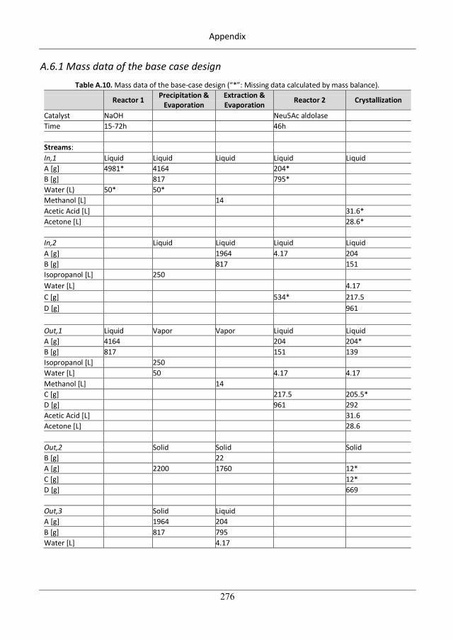
Appendix
276
A.6.1 Mass data of the base case design Table A.10. Mass data of the base-case design (“*”: Missing data calculated by mass balance).
Reactor 1 Precipitation & Evaporation
Extraction & Evaporation Reactor 2 Crystallization
Catalyst NaOH Neu5Ac aldolase Time 15-72h 46h Streams: In,1 Liquid Liquid Liquid Liquid Liquid A [g] 4981* 4164 204* B [g] 817 795* Water (L) 50* 50* Methanol [L] 14 Acetic Acid [L] 31.6* Acetone [L] 28.6* In,2 Liquid Liquid Liquid Liquid A [g] 1964 4.17 204 B [g] 817 151 Isopropanol [L] 250 Water [L] 4.17 C [g] 534* 217.5 D [g] 961 Out,1 Liquid Vapor Vapor Liquid Liquid A [g] 4164 204 204* B [g] 817 151 139 Isopropanol [L] 250 Water [L] 50 4.17 4.17 Methanol [L] 14 C [g] 217.5 205.5* D [g] 961 292 Acetic Acid [L] 31.6 Acetone [L] 28.6 Out,2 Solid Solid Solid B [g] 22 A [g] 2200 1760 12* C [g] 12* D [g] 669 Out,3 Solid Liquid A [g] 1964 204 B [g] 817 795 Water [L] 4.17
306
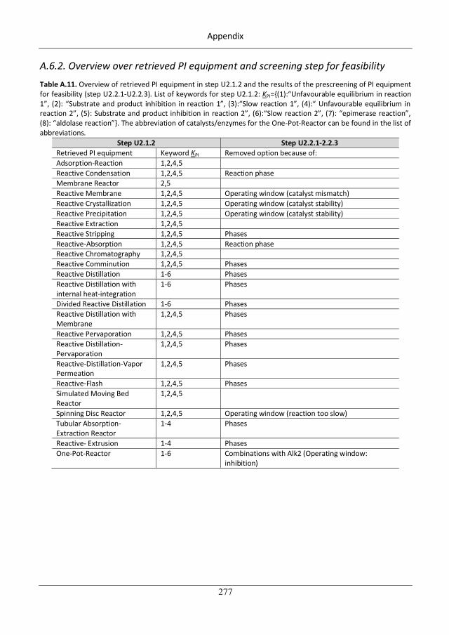
Appendix
277
A.6.2. Overview over retrieved PI equipment and screening step for feasibility Table A.11. Overview of retrieved PI equipment in step U2.1.2 and the results of the prescreening of PI equipment for feasibility (step U2.2.1-U2.2.3). List of keywords for step U2.1.2: KPI={(1):“Unfavourable equilibrium in reaction 1”, (2): “Substrate and product inhibition in reaction 1”, (3):“Slow reaction 1”, (4):“ Unfavourable equilibrium in reaction 2”, (5): Substrate and product inhibition in reaction 2”, (6):“Slow reaction 2”, (7): “epimerase reaction”, (8): “aldolase reaction”}. The abbreviation of catalysts/enzymes for the One-Pot-Reactor can be found in the list of abbreviations.
Step U2.1.2 Step U2.2.1-2.2.3 Retrieved PI equipment Keyword KPI Removed option because of: Adsorption-Reaction 1,2,4,5 Reactive Condensation 1,2,4,5 Reaction phase Membrane Reactor 2,5 Reactive Membrane 1,2,4,5 Operating window (catalyst mismatch) Reactive Crystallization 1,2,4,5 Operating window (catalyst stability) Reactive Precipitation 1,2,4,5 Operating window (catalyst stability) Reactive Extraction 1,2,4,5 Reactive Stripping 1,2,4,5 Phases Reactive-Absorption 1,2,4,5 Reaction phase Reactive Chromatography 1,2,4,5 Reactive Comminution 1,2,4,5 Phases Reactive Distillation 1-6 Phases Reactive Distillation with internal heat-integration
1-6 Phases
Divided Reactive Distillation 1-6 Phases Reactive Distillation with Membrane
1,2,4,5 Phases
Reactive Pervaporation 1,2,4,5 Phases Reactive Distillation-Pervaporation
1,2,4,5 Phases
Reactive-Distillation-Vapor Permeation
1,2,4,5 Phases
Reactive-Flash 1,2,4,5 Phases Simulated Moving Bed Reactor
1,2,4,5
Spinning Disc Reactor 1,2,4,5 Operating window (reaction too slow) Tubular Absorption-Extraction Reactor
1-4 Phases
Reactive- Extrusion 1-4 Phases One-Pot-Reactor 1-6 Combinations with Alk2 (Operating window:
inhibition)
307
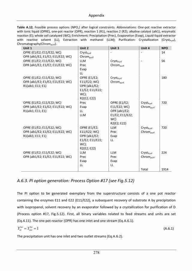
Appendix
278
Table A.12. Feasible process options (NPOL) after logical constraints. Abbreviations: One-pot reactive extractor with ionic liquid (OPRE), one-pot reactor (OPR), reaction 1 (R1), reaction 2 (R2); alkaline catalyst (alk1), enzymatic reaction (E); whole cell catalyzed (WC); Enrichment: Precipitation (Prec), Evaporation (Evap), Liquid-liquid extractor with reactive solvent (LL), Extraction with methanol (LLM); Purification: Crystallization (CrystPurif), Chromatography(Chrompurif).
Unit 1 Unit 2 Unit 3 Unit 4 NPO OPRE (E1/E2; E11/E22; WC) OPR (alk1/E2, E1/E2; E11/E22; WC)
CrystPurif
Chrompurif - - 14
OPRE (E1/E2; E11/E22; WC) OPR (alk1/E2, E1/E2; E11/E22; WC)
LLM Prec Evap LL
CrystPurif
Chrompurif - 56
OPRE (E1/E2; E11/E22; WC) OPR (alk1/E2; E1/E2; E11/E22; WC) R1(alk1; E11; E1)
OPRE (E1/E2; E11/E22; WC) OPR (alk1/E2; E1/E2; E11/E22; WC); R2(E2; E22)
CrystPurif
Chrompurif 180
OPRE (E1/E2; E11/E22; WC) OPR (alk1/E2; E1/E2; E11/E22; WC) R1(alk1; E11; E1)
Prec Evap LL LLM
OPRE (E1/E2; E11/E22; WC) OPR (alk1/E2; E1/E2; E11/E22; WC) R2(E2; E22)
CrystPurif
Chrompurif 720
OPRE (E1/E2; E11/E22; WC) OPR (alk1/E2; E1/E2; E11/E22; WC) R1(alk1; E11; E1)
OPRE (E1/E2; E11/E22; WC) OPR (alk1/E2; E1/E2; E11/E22; WC); R2(E2; E22)
LLM Prec Evap LL
CrystPurif
Chrompurif 720
OPRE (E1/E2; E11/E22; WC) OPR (alk1/E2; E1/E2; E11/E22; WC)
LLM Prec Evap LL
LLM Prec Evap LL
CrystPurif
Chrompurif
224
Total 1914
A.6.3. PI option generation: Process Option #17 (see Fig.5.12)
The PI option to be generated exemplary from the superstructure consists of a one pot reactor
containing the enzymes E11 and E22 (E11/E22), a subsequent recovery of substrate A by precipitation
with isopropanol, solvent recovery by an evaporator followed by a crystallization for purification of D
(Process option #17, Fig.5.12). First, all binary variables related to feed streams and units are set
(Eq.4.11). The one pot-reactor (OPR) has one inlet and one stream (Eq.A.6.1). 1 1 1in outY Y (A.6.1)
The precipitation unit has one inlet and two outlet streams (Eq.A.6.2).
308
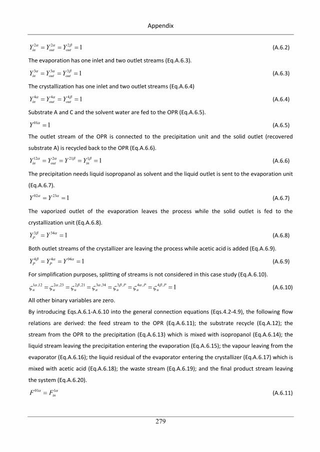
Appendix
279
2 2 2 1in out outY Y Y (A.6.2)
The evaporation has one inlet and two outlet streams (Eq.A.6.3). 3 3 3 1in out outY Y Y (A.6.3)
The crystallization has one inlet and two outlet streams (Eq.A.6.4) 4 4 4 1in out outY Y Y (A.6.4)
Substrate A and C and the solvent water are fed to the OPR (Eq.A.6.5). 01 1Y (A.6.5)
The outlet stream of the OPR is connected to the precipitation unit and the solid outlet (recovered
substrate A) is recycled back to the OPR (Eq.A.6.6). 12 2 21 1 1in out inY Y Y Y (A.6.6)
The precipitation needs liquid isopropanol as solvent and the liquid outlet is sent to the evaporation unit
(Eq.A.6.7). 02 23 1Y Y (A.6.7)
The vaporized outlet of the evaporation leaves the process while the solid outlet is fed to the
crystallization unit (Eq.A.6.8). 3 34 1PY Y (A.6.8)
Both outlet streams of the crystallizer are leaving the process while acetic acid is added (Eq.A.6.9). 4 4 04 1P PY Y Y (A.6.9)
For simplification purposes, splitting of streams is not considered in this case study (Eq.A.6.10). 1 ,12 2 ,23 2 ,21 3 ,34 3 , 4 , 4 , 1P P Pu u u u u u u (A.6.10)
All other binary variables are zero.
By introducing Eqs.A.6.1-A.6.10 into the general connection equations (Eqs.4.2-4.9), the following flow
relations are derived: the feed stream to the OPR (Eq.A.6.11); the substrate recycle (Eq.A.12); the
stream from the OPR to the precipitation (Eq.A.6.13) which is mixed with isopropanol (Eq.A.6.14); the
liquid stream leaving the precipitation entering the evaporation (Eq.A.6.15); the vapour leaving from the
evaporator (Eq.A.6.16); the liquid residual of the evaporator entering the crystallizer (Eq.A.6.17) which is
mixed with acetic acid (Eq.A.6.18); the waste stream (Eq.A.6.19); and the final product stream leaving
the system (Eq.A.6.20). 01 1
inF F (A.6.11)
309
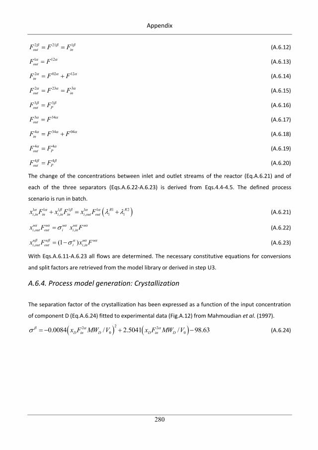
Appendix
280
2 21 1out inF F F (A.6.12)
1 12outF F (A.6.13)
2 02 12inF F F (A.6.14)
2 23 3out inF F F (A.6.15)
3 3out PF F (A.6.16)
3 34outF F (A.6.17)
4 34 04inF F F (A.6.18)
4 4out PF F (A.6.19)
4 4out PF F (A.6.20)
The change of the concentrations between inlet and outlet streams of the reactor (Eq.A.6.21) and of
each of the three separators (Eqs.A.6.22-A.6.23) is derived from Eqs.4.4-4.5. The defined process
scenario is run in batch.
1 1 1 1 1 1 1 2, , ,
R Ri in in i in in i out out i ix F x F x F (A.6.21)
, ,u u u u ui out out i i inx F x F (A.6.22)
, ,(1 )u u u ui out out i i inx F x F (A.6.23)
With Eqs.A.6.11-A.6.23 all flows are determined. The necessary constitutive equations for conversions
and split factors are retrieved from the model library or derived in step U3.
A.6.4. Process model generation: Crystallization
The separation factor of the crystallization has been expressed as a function of the input concentration
of component D (Eq.A.6.24) fitted to experimental data (Fig.A.12) from Mahmoudian et al. (1997). 22 2
0 00.0084 / 2.5041 / 98.63D in D D in Dx F MW V x F MW V (A.6.24)
310
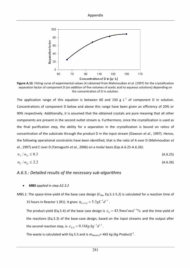
Appendix
281
Figure A.12. Fitting curve of experimental values (•) obtained from Mahmoudian et al. (1997) for the crystallization
separation factor of component D (on addition of five volumes of acetic acid to aqueous solutions) depending on the concentration of D in solution.
The application range of this equation is between 60 and 150 g L-1 of component D in solution.
Concentrations of component D below and above this range have been given an efficiency of 20% or
90% respectively. Additionally, it is assumed that the obtained crystals are pure meaning that all other
components are present in the second outlet stream . Furthermore, since the crystallization is used as
the final purification step, the ability for a separation in the crystallization is bound on ratios of
concentration of the substrate through the product D in the input stream (Dawson et al., 1997). Hence,
the following operational constraints have been identified, that is the ratio of A over D (Mahmoudian et
al., 1997) and C over D (Yamaguchi et al., 2006) on a molar basis (Eqs.A.6.25-A.6.26):
3.0/ DA nn (A.6.25)
2.2/ DC nn (A.6.26)
A.6.5.: Detailed results of the necessary sub-algorithms
MBS applied in step A2.3.2
MBS.1: The space-time-yield of the base case design (FObj, Eq.5.1-5.2) is calculated for a reaction time of
15 hours in Reactor 1 (R1). It gives 1 1,15,0 5.3P gL d .
The product-yield (Eq.5.4) of the base case design is 10 43.9 %mol mol and the time-yield of
the reactions (Eq.5.3) of the base-case design, based on the input streams and the output after
the second reaction step, is 1 1,0 0.16R kg kg d .
The waste is calculated with Eq.5.5 and is mWaste,0= 465 kg (kg Product)-1.
311
Appendix
282
MBS.2: Main contributors to the objective function are identified to be both reaction steps (due to long
residence times and low conversions: 01 0.2R and 0
1 0.9R , see Eq.3.5, Table 3.2; section
3.3.2) as well as the last separation (low efficiency: Cryst=0.7). The main contributors of waste are
the solvent (isopropanol) for precipitation (250 L) and the high amount of water necessary to
dilute the substrates (50 L). Therefore, they are added to the list of limitations/bottlenecks:
LB={LB1:“Low conversion in reaction 1”, LB2:“Slow reaction 1”, LB3:“Low conversion in reaction 2”,
LB4:“Slow reaction 2”, LB5:“Low productivity/efficiency in separating D/CAB”, LB6:“High waste
generation for enrichment of B”, LB7:“High waste generation due to high dilution of substrates”}.
MBS.3: The time-yield for each reaction (Eq.5.3) is calculated: 1 11,0 0.26R kg kg day and
1 12,0 0.36R kg kg day . Both reaction tasks are violating the operational constraint
( 1 10.75R kg kg day , see Table 5.1). Hence, they are identified to be responsible for a
limitation. However, there are already included in the list of LB (step MBS.2).
MBS.4: This step is not necessary.
APCP in step A2.4.1
APCP.1: The workflow given by the sub-steps APCP.1.1-APCP.1.3 is used to generate/retrieve pure
component properties PCP. All details are presented in Table 5.2.
APCP.2: The results are presented in Table 5.3.
APCP.3: The results are presented in Table 5.4.
APCP.4: By applying the rules, the following limitations/bottlenecks are explained: The
limitation/bottleneck LB5 is explained by the low difference in the pKa-value of D and C (Rule
APCP.1). The difference in the solubility in water Log(Ws) and the octanol-water partition
coefficient Log(Kow) between the components (important for mixing phenomena in the tasks
responsible for LB1-LB7) needs further investigation for an occurrence of miscibility gaps (Rule
APCP.2).
AMP in step A2.4.2
AMP.1: Azeotropes (Rule AMP.1) and solubility (Rule AMP.2) are identified to be necessary mixture
properties to be investigated in more detail.
312
Appendix
283
AMP.2: No azeotrope is found. The solubilities of the components are retrieved from Blayer et al., 1999.
The solubilities in water are 1.3 mol L-1 for A, 3.6 mol L-1 for C, 1 mol L-1 for D while the solubility
for B depends on the concentration of C.
AMP.3: Compute azeotropes and/or miscibility gaps using thermodynamic models describing the
involved phases:
AMP.3.1: All information is available, therefore step AMP.5 is entered (Rule AMP.5).
AMP.5: The low solubilities of the components explain (Rule AMP.7) the large amount of solvents
needed which are responsible for limitation/bottleneck LB6-LB7.
AR in step A2.4.3
AR.1: Both reactions are responsible for limitations LB1-LB4 in the base-case design, the AR algorithm is
applied (Rule AR.1).
AR.2 Collect data for reaction analysis:
AR.2.1: The equilibrium constants are retrieved from the literature and are KEQ,R1=0.24 and
KEQ,R2=28.7 L mol-1 (Zimmermann et al., 2007).
AR.2.2: The reaction times are given in Table A.9.
AR.2.3: The determination of the heat of reaction is not required (Rule AR.2), step AR.3 is entered.
AR.3 The theoretical equilibrium conversion of the reactions at the operating conditions with equimolar
substrates are 01, 0.2R EQ and 0
2, 0.87R EQ .
AR.4: The deviation of actual and theoretical calculated conversions is low: 1 0R and 2 0.03R .
AR.5: Reaction 1 and reaction 2 are both limited due to an unfavourable equilibrium (criterion 1,
Table 3.3) and a slow reaction (criterion 6, Table 3.3).
AR.6: Inhibition might be possible (criterion 1, Table 3.3), hence, step AR.7 is entered.
AR.7: The first reaction is inhibited (LB8) by the product D and the substrate C while the second reaction
is inhibited (LB9) by the substrates B and C as well as A (Zimmermann et al., 2007).
A.7. Additional material to the case study: H2O2 (section 5.2)
In this section, additional tables for the solution of case study to produce hydrogen peroxide via
anthraquinone route (section 5.2) are given. It includes the mass and energy data of the base case
design (Table A.13), the identified limitations/bottlenecks of this base case design (Table A.14) as well as
the list of retrieved PI equipment to overcome these limitations for process improvement (Table A.15).
313
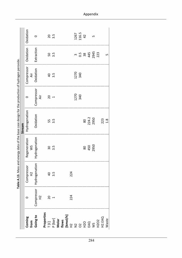
Appendix
284
Tabl
e A.
13. M
ass a
nd e
nerg
y da
ta o
f the
bas
e ca
se d
esig
n fo
r the
pro
duct
ion
of h
ydro
gen
pero
xide
. St
ream
Co
min
g fr
om
0 Co
mpr
esso
r H2
Re
gene
ratio
n W
S Hy
drog
enat
ion
0 Co
mpr
esso
r Ai
r O
xida
tion
Oxi
datio
n
Goin
g to
Co
mpr
esso
r H2
Hy
drog
enat
ion
Hydr
ogen
atio
n O
xida
tion
Com
pres
sor
Air
Oxi
datio
n Ex
trac
tion
0
Prop
ertie
s
T
[C]
20
40
30
55
20
40
50
20
P [b
ar]
1 3.
5 3.
5 3.
5 1
3.5
3.5
3.5
Mol
ar
flow
s [k
mol
/h]
H2
224
224
N2
1270
12
70
3 12
67
O2
340
340
0.5
116.
5 H2
O
80
80
38
42
EAQ
45
0 22
4.2
445
W
S
29
50
2950
29
45
5 H2
O2
223
H2
.EAQ
223
Was
te
1.
8
5
314
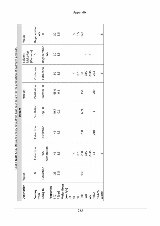
Appendix
285
Cont
.d T
able
A.1
3. M
ass a
nd e
nerg
y da
ta o
f the
bas
e ca
se d
esig
n fo
r the
pro
duct
ion
of h
ydro
gen
pero
xide
. St
ream
De
scrip
tion
Wat
er
Pr
oduc
t
Solv
ent
Mak
e -U
p (Q
uino
ne)
Was
te
Com
ing
from
0
Extr
actio
n Ex
trac
tion
Dist
illat
ion
Dist
illat
ion
Oxi
datio
n 0
Rege
nera
tion
WS
Goin
g to
Ex
trac
tion
WS
Gene
ratio
n Di
still
atio
n To
p - 0
Bo
ttom
- 0
Extr
actio
n Re
gene
ratio
n W
S 0
Prop
ertie
s
T
[C]
35
49
49
49.7
65
.0
50
30
30
P [b
ar]
3.5
3.5
4.5
0.1
0.1
3.5
3.5
3.5
Mol
ar fl
ows
[km
ol/h
]
H2
N2
3
3
3
O2
0.
5
0.5
0.
5 H2
O
930
208
760
609
151
38
12
8 EA
Q
44
5
445
5
WS
29
45
29
45
5
H2O
2
13
210
1 20
9 22
3
H2
.EAQ
W
aste
5
5
5
315
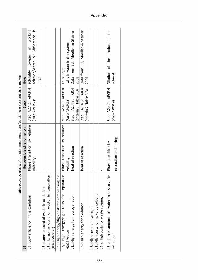
Appendix
286
Tabl
e A.
14. O
verv
iew
of t
he id
entif
ied
limita
tions
/bot
tlene
cks (
LB) a
nd th
eir a
naly
sis.
LB
Resp
onsib
le p
heno
men
on
Step
Ho
w
LB1:
Low
effi
cien
cy in
the
oxid
atio
n Ph
ase
tran
sitio
n by
rel
ativ
e vo
latil
ity
Step
A2.
4.1:
APC
P.4
( Rul
e AP
CP.7
):
solu
bilit
y ox
ygen
in
w
orki
ng
solu
tion/
wat
er
VP
diffe
renc
e is
larg
e LB
2: La
rge
amou
nt o
f was
te in
oxi
datio
n -
LB3:
Larg
e am
ount
of
w
aste
in
se
para
tion
(H2O
2/W
ater
) -
LB4:
High
ene
rgy/
High
cost
s for
com
pres
sing
air
-
LB
5: Hi
gh
ener
gy/H
igh
cost
s fo
r se
para
tion
H2O
2/w
ater
Ph
ase
tran
sitio
n by
rel
ativ
e vo
latil
ity
Step
A2.
4.1:
APC
P.4
(Rul
e AP
CP.1
) Tb
is la
rge
why
is w
ater
in th
e sy
stem
LB
6: Hi
gh e
nerg
y fo
r hyd
roge
natio
n;
heat
of r
eact
ion
Step
A2
.4.3
: AR
.4
(crit
eria
2, T
able
3.3
) Da
ta f
rom
Eul
, Moe
ller
& S
tein
er,
2001
LB
7: Hi
gh e
nerg
y fo
r oxi
datio
n he
at o
f rea
ctio
n St
ep
A2.4
.3:
AR.4
(c
riter
ia 2
, Tab
le 3
.3)
Data
fro
m E
ul, M
oelle
r &
Ste
iner
, 20
01
LB8:
High
cost
s for
hyd
roge
n -
LB9:
High
cost
s for
mak
e-up
solv
ent
-
LB
10: H
igh
cost
s for
was
te st
ream
; -
LB11
: La
rge
amou
nt o
f w
ater
nec
essa
ry f
or
extr
actio
n Ph
ase
tran
sitio
n by
extr
actio
n an
d m
ixin
g
Step
A2.
4.1:
APC
P.4
(Rul
e AP
CP.9
) Di
lutio
n of
th
e pr
oduc
t in
th
e so
lven
t
316
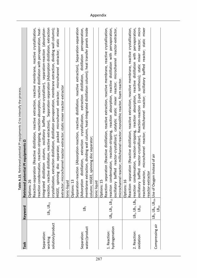
Appendix
287
Tabl
e A.
15. R
etrie
ved
pote
ntia
l PI e
quip
men
ts
to in
tens
ify th
e pr
oces
s.
Task
Ke
ywor
d
Retr
ieve
d po
tent
ial P
I equ
ipm
ents
Sepa
ratio
n:
wor
king
so
lutio
n/pr
oduc
t LB
3, LB
11
Opt
ions
: 26
Re
actio
n -se
para
tion
(Rea
ctiv
e di
still
atio
n, r
eact
ive
extr
actio
n, r
eact
ive
mem
bran
e, r
eact
ive
crys
talli
zatio
n,
reac
tion
cond
ensa
tion,
reac
tion-
strip
ping
, rea
ctio
n-ab
sorp
tion,
reac
tive
dist
illat
ion
with
per
vapo
ratio
n, h
eat-
inte
grat
ed d
istill
atio
n co
lum
n, o
scill
ator
y ba
ffled
rea
ctor
-cry
stal
lizer
), se
para
tion-
reac
tion
(abs
orpt
ion-
reac
tion,
reac
tive
dist
illat
ion,
reac
tive
extr
actio
n),
Sep
arat
ion -
sepa
ratio
n (A
dsor
ptio
n di
still
atio
n, e
xtra
ctio
n cr
ysta
lliza
tion,
ext
ract
ion
dist
illat
ion,
dist
illat
ion
perv
apor
atio
n, m
embr
ane
extr
actio
n, d
ivid
ing
wal
l col
umn)
; HI
GEE,
spi
nnin
g di
sc s
epar
ator
; pa
cked
mic
roch
anne
l ex
trac
tor;
mic
roch
anne
l ex
trac
tor;
stat
ic m
ixer
ex
trac
tor;
mic
roch
anne
l rea
ctor
-ext
ract
or; s
tatic
mix
er re
acto
r-ex
trac
tor
Ioni
c-liq
uid
Sepa
ratio
n:
wat
er/p
rodu
ct
LB5
Opt
ions
: 13
Sepa
ratio
n -re
actio
n (A
bsor
ptio
n-re
actio
n, r
eact
ive
dist
illat
ion,
rea
ctiv
e ex
trac
tion)
, Se
para
tion-
sepa
ratio
n (A
dsor
ptio
n di
still
atio
n,
extr
actio
n cr
ysta
lliza
tion,
ex
trac
tion
dist
illat
ion,
di
still
atio
n pe
rvap
orat
ion,
m
embr
ane
extr
actio
n, d
ivid
ing
wal
l col
umn,
hea
t-in
tegr
ated
dist
illat
ion
colu
mn)
; hea
t tra
nsfe
r pan
els
insid
e co
lum
n; H
IGEE
, spi
nnin
g di
sc se
para
tor;
Io
nic l
iqui
d
1. R
eact
ion:
hy
drog
enat
ion
LB6,
LB1,
LB12
Opt
ions
: 15
Reac
tion-
sep
arat
ion
(Rea
ctiv
e di
still
atio
n, r
eact
ive
extr
actio
n, r
eact
ive
mem
bran
e, r
eact
ive
crys
talli
zatio
n,
reac
tion
cond
ensa
tion,
rea
ctio
n -st
rippi
ng,
reac
tion
abso
rptio
n, r
eact
ive
dist
illat
ion
with
per
vapo
ratio
n,
osci
llato
ry
baffl
ed
reac
tor-
crys
talli
zer)
; ca
taly
tic
stat
ic
mix
er
reac
tor;
mic
roch
anne
l re
acto
r-ex
trac
tor,
mic
roch
anne
l rea
ctor
; mill
icha
nnel
reac
tor;
mon
olith
ic re
acto
r, fo
am re
acto
r.
2. R
eact
ion:
ox
idat
ion
LB1,
LB7,
LB9,
LB13
Opt
ions
: 16
Reac
tion-
sep
arat
ion
(Rea
ctiv
e di
still
atio
n, r
eact
ive
extr
actio
n, r
eact
ive
mem
bran
e, r
eact
ive
crys
talli
zatio
n,
reac
tion
cond
ensa
tion,
rea
ctio
n-st
rippi
ng,
reac
tion
abso
rptio
n, r
eact
ive
dist
illat
ion
with
per
vapo
ratio
n,
osci
llato
ry b
affle
d re
acto
r-cr
ysta
llize
r),
Reac
tion-
reac
tion
(1-p
ot s
ynth
esis)
; st
atic
mix
er r
eact
or;
mic
ro
reac
tor-
extr
acto
r, m
icro
chan
nel
reac
tor;
mill
icha
nnel
rea
ctor
; os
cilla
tory
baf
fled
reac
tor;
stat
ic m
ixer
re
acto
r-ex
trac
tor
Com
pres
sing
air
LB2,
LB4,
LB10
, LB
14
Use
of O
xyge
n in
stea
d of
air
317
Appendix
288
A.8. Additional material to the case study: HMF (section 5.3)
In this section, additional material to solve the case study to produce HMD (section 5.3) is given. It
includes the mass and energy data of the base-case design of Rapp (1988) given in section A.8.1, the
superstructure containing all options satisfying operational constraints and performance metrics using
simple models (A.8.2) as well as the selection of solvents for the reactive extraction units by applying
sub-algorithm SoP is shown in detail (A.8.3).
A.8.1 Mass and energy data of the base-case design
318
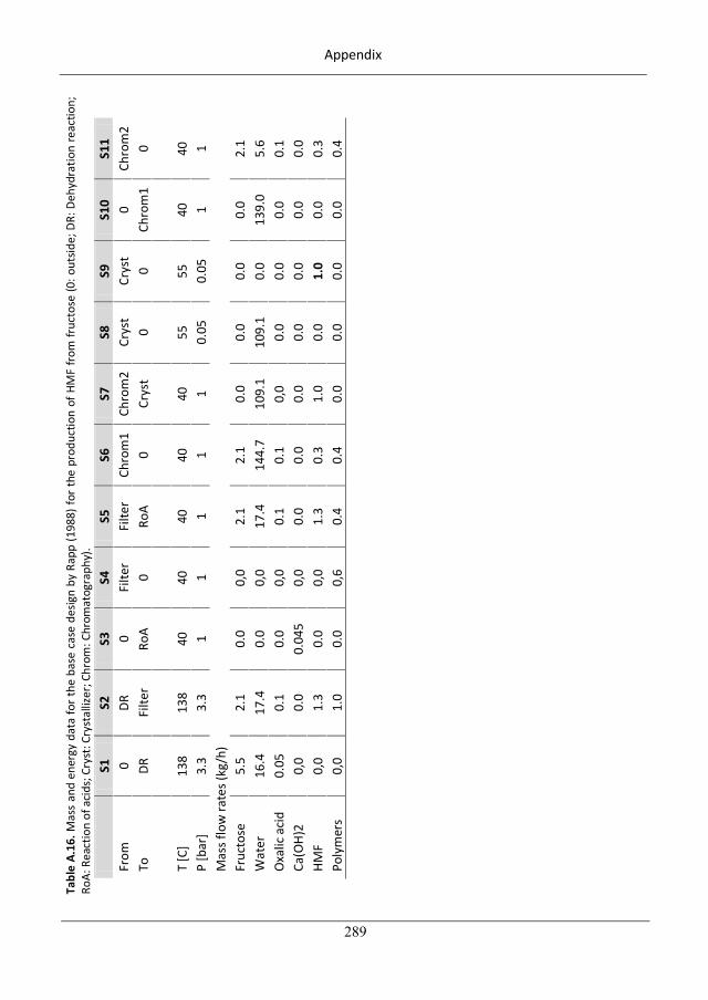
Appendix
289
Tabl
e A.
16. M
ass
and
ener
gy d
ata
for t
he b
ase
case
des
ign
by R
app
(198
8) fo
r th
e pr
oduc
tion
of H
MF
from
fruc
tose
(0: o
utsid
e; D
R: D
ehyd
ratio
n re
actio
n;
RoA:
Rea
ctio
n of
aci
ds; C
ryst
: Cry
stal
lizer
; Chr
om: C
hrom
atog
raph
y).
S1
S2
S3
S4
S5
S6
S7
S8
S9
S1
0 S1
1 Fr
om
0 DR
0
Filte
r Fi
lter
Chro
m1
Chro
m2
Crys
t Cr
yst
0 Ch
rom
2 To
DR
Fi
lter
RoA
0 Ro
A 0
Crys
t 0
0 Ch
rom
1 0
T [C
] 13
8 13
8 40
40
40
40
40
55
55
40
40
P
[bar
] 3.
3 3.
3 1
1 1
1 1
0.05
0.
05
1 1
Mas
s flo
w ra
tes (
kg/h
) Fr
ucto
se
5.5
2.1
0.0
0,0
2.1
2.1
0.0
0.0
0.0
0.0
2.1
Wat
er
16.4
17
.4
0.0
0,0
17.4
14
4.7
109.
1 10
9.1
0.0
139.
0 5.
6 O
xalic
aci
d 0.
05
0.1
0.0
0,0
0.1
0.1
0,0
0.0
0.0
0.0
0.1
Ca(O
H)2
0,0
0.0
0.04
5 0,
0 0.
0 0.
0 0.
0 0.
0 0.
0 0.
0 0.
0 HM
F 0,
0 1.
3 0.
0 0,
0 1.
3 0.
3 1.
0 0.
0 1.
0 0.
0 0.
3 Po
lym
ers
0,0
1.0
0.0
0,6
0.4
0.4
0.0
0.0
0.0
0.0
0.4
319

Appendix
290
A.8.2. Superstructure of the remaining options after screening for operational
constraints and performance metric using simple models
320
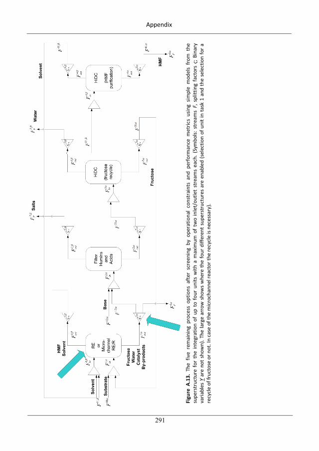
Appendix
291
Fi
gure
A.1
3. T
he f
ive
rem
aini
ng p
roce
ss o
ptio
ns a
fter
scr
eeni
ng b
y op
erat
iona
l co
nstr
aint
s an
d pe
rfor
man
ce m
etric
s us
ing
simpl
e m
odel
s fr
om t
he
supe
rstr
uctu
re f
or t
he in
tegr
atio
n of
up
to f
our
units
with
a m
axim
um o
f tw
o in
let/
outle
t st
ream
s ea
ch. (
Sym
bols:
str
eam
s F,
spl
ittin
g fa
ctor
s ; B
inar
y va
riabl
es Y
are
not
sho
wn)
. The
larg
e ar
row
sho
ws
whe
re th
e fo
ur d
iffer
ent s
uper
stru
ctur
es a
re e
nabl
ed (s
elec
tion
of u
nit i
n ta
sk 1
and
the
sele
ctio
n fo
r a
recy
cle
of fr
ucto
se o
r not
. In
case
of t
he m
icro
chan
nel r
eact
or th
e re
cycl
e is
nece
ssar
y).
321
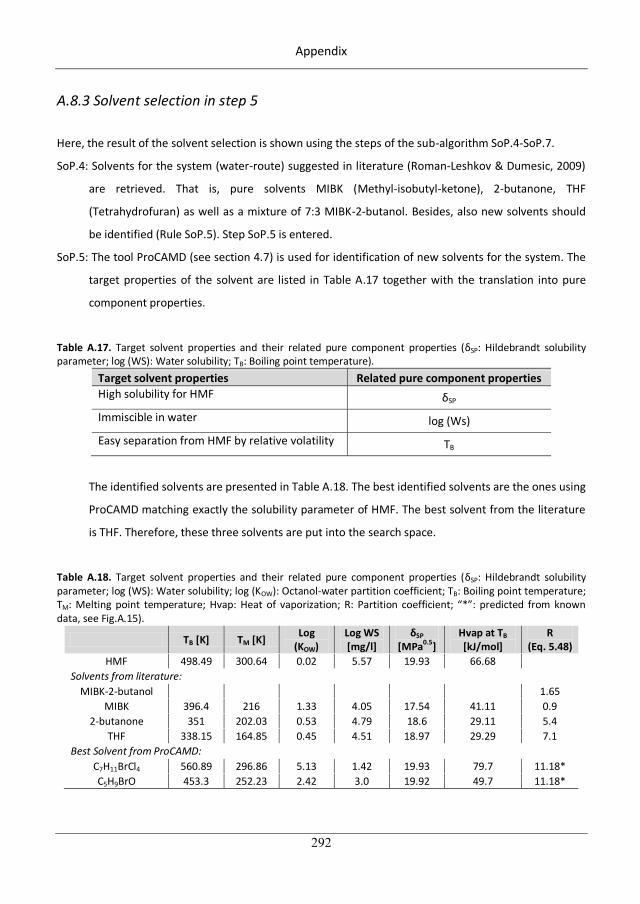
Appendix
292
A.8.3 Solvent selection in step 5
Here, the result of the solvent selection is shown using the steps of the sub-algorithm SoP.4-SoP.7.
SoP.4: Solvents for the system (water-route) suggested in literature (Roman-Leshkov & Dumesic, 2009)
are retrieved. That is, pure solvents MIBK (Methyl-isobutyl-ketone), 2-butanone, THF
(Tetrahydrofuran) as well as a mixture of 7:3 MIBK-2-butanol. Besides, also new solvents should
be identified (Rule SoP.5). Step SoP.5 is entered.
SoP.5: The tool ProCAMD (see section 4.7) is used for identification of new solvents for the system. The
target properties of the solvent are listed in Table A.17 together with the translation into pure
component properties.
Table A.17. Target solvent properties and their related pure component properties ( SP: Hildebrandt solubility parameter; log (WS): Water solubility; TB: Boiling point temperature).
Target solvent properties Related pure component properties High solubility for HMF
SP Immiscible in water log (Ws) Easy separation from HMF by relative volatility TB
The identified solvents are presented in Table A.18. The best identified solvents are the ones using
ProCAMD matching exactly the solubility parameter of HMF. The best solvent from the literature
is THF. Therefore, these three solvents are put into the search space.
Table A.18. Target solvent properties and their related pure component properties ( SP: Hildebrandt solubility parameter; log (WS): Water solubility; log (KOW): Octanol-water partition coefficient; TB: Boiling point temperature; TM: Melting point temperature; Hvap: Heat of vaporization; R: Partition coefficient; “*”: predicted from known data, see Fig.A.15).
TB [K] TM [K] Log (KOW)
Log WS [mg/l]
SP
[MPa0.5] Hvap at TB [kJ/mol]
R (Eq. 5.48)
HMF 498.49 300.64 0.02 5.57 19.93 66.68 Solvents from literature:
MIBK-2-butanol 1.65 MIBK 396.4 216 1.33 4.05 17.54 41.11 0.9
2-butanone 351 202.03 0.53 4.79 18.6 29.11 5.4 THF 338.15 164.85 0.45 4.51 18.97 29.29 7.1
Best Solvent from ProCAMD: C7H11BrCl4 560.89 296.86 5.13 1.42 19.93 79.7 11.18* C5H9BrO 453.3 252.23 2.42 3.0 19.92 49.7 11.18*
322
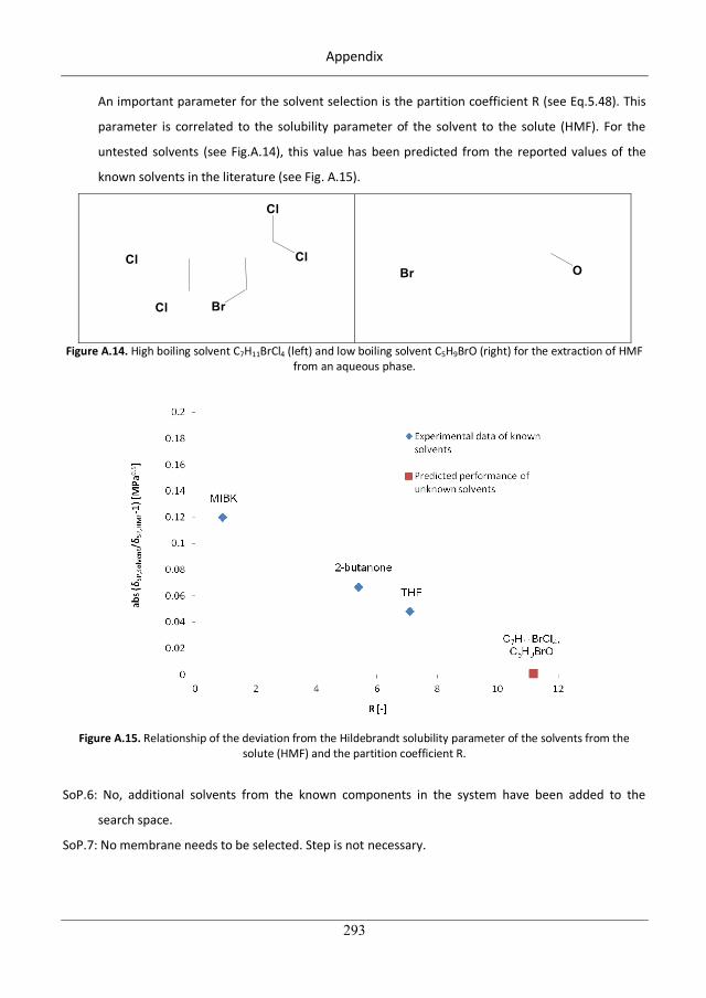
Appendix
293
An important parameter for the solvent selection is the partition coefficient R (see Eq.5.48). This
parameter is correlated to the solubility parameter of the solvent to the solute (HMF). For the
untested solvents (see Fig.A.14), this value has been predicted from the reported values of the
known solvents in the literature (see Fig. A.15).
Cl Cl
Cl
BrCl
Br O
Figure A.14. High boiling solvent C7H11BrCl4 (left) and low boiling solvent C5H9BrO (right) for the extraction of HMF from an aqueous phase.
Figure A.15. Relationship of the deviation from the Hildebrandt solubility parameter of the solvents from the
solute (HMF) and the partition coefficient R.
SoP.6: No, additional solvents from the known components in the system have been added to the
search space.
SoP.7: No membrane needs to be selected. Step is not necessary.
323
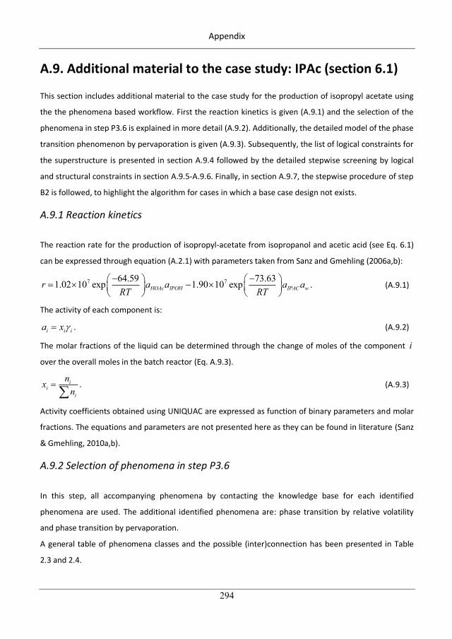
Appendix
294
A.9. Additional material to the case study: IPAc (section 6.1)
This section includes additional material to the case study for the production of isopropyl acetate using
the the phenomena based workflow. First the reaction kinetics is given (A.9.1) and the selection of the
phenomena in step P3.6 is explained in more detail (A.9.2). Additionally, the detailed model of the phase
transition phenomenon by pervaporation is given (A.9.3). Subsequently, the list of logical constraints for
the superstructure is presented in section A.9.4 followed by the detailed stepwise screening by logical
and structural constraints in section A.9.5-A.9.6. Finally, in section A.9.7, the stepwise procedure of step
B2 is followed, to highlight the algorithm for cases in which a base case design not exists.
A.9.1 Reaction kinetics
The reaction rate for the production of isopropyl-acetate from isopropanol and acetic acid (see Eq. 6.1)
can be expressed through equation (A.2.1) with parameters taken from Sanz and Gmehling (2006a,b):
7 764.59 73.631.02 10 exp 1.90 10 expHOAc IPOH IPAC wr a a a aRT RT
. (A.9.1)
The activity of each component is:
i i ia x . (A.9.2)
The molar fractions of the liquid can be determined through the change of moles of the component i
over the overall moles in the batch reactor (Eq. A.9.3).
ii
i
nxn
. (A.9.3)
Activity coefficients obtained using UNIQUAC are expressed as function of binary parameters and molar
fractions. The equations and parameters are not presented here as they can be found in literature (Sanz
& Gmehling, 2010a,b).
A.9.2 Selection of phenomena in step P3.6
In this step, all accompanying phenomena by contacting the knowledge base for each identified
phenomena are used. The additional identified phenomena are: phase transition by relative volatility
and phase transition by pervaporation.
A general table of phenomena classes and the possible (inter)connection has been presented in Table
2.3 and 2.4.
324
Appendix
295
The detailed selection procedure is presented in table A.19 and is here briefly explained for the first two
phenomena. Since, this procedure is an iterative procedure; the first selection is abbreviated with S1,
the second with S2, and so on.
S1: The first phenomenon in the search space is the reaction taking place in the liquid phase. Hence,
liquid phase mixing phenomena need to be selected. Additional, a stream dividing phenomenon is by
definition also always selected. The reaction is exothermic. Hence, cooling and heating phenomena are
selected. This selection can be followed by looking at the reaction phenomenon in the first row and the
second last column (Table A.19). Moving this column downwards, the abbreviation S1 is put for each
phenomenon selected. Following this column downwards, all selected phenomena are marked.
S2: The second phenomenon in the search space is the phase transition phenomenon by relative
volatility. For occurrence, a phase contact and thermal heat/cooling are necessary as well as a suitable
phase separation phenomenon (Table 2.4). Hence, for all of these suitable V-L phenomena are selected
(Table A.19).
The procudre stops when all phenomena in the search spce have been the basis for a search. In total 12
repetitive steps (S1-S12) are necessary, giving in total a number of 12 phenomena (PB.1-PB.12). The
selected phenomena are presented in Table A.20.
325
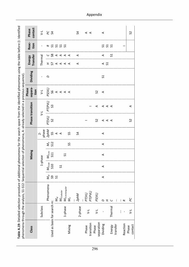
Appendix
296
Tabl
e A.
19: D
etai
led
sele
ctio
n pr
oced
ure
of a
dditi
onal
phe
nom
ena
for t
he s
earc
h sp
ace
from
the
iden
tifie
d ph
enom
ena
usin
g th
e ta
ble
befo
re (I
: Ide
ntifi
ed
phen
omen
a th
roug
h th
e an
alys
is, S
1-S1
2: S
eque
ntia
l sel
ectio
n of
phe
nom
ena,
A: a
lread
y se
lect
ed in
a p
revi
ous s
eque
nce)
.
Clas
s
M
ixin
g Ph
ase
tran
sitio
n Ph
ase
sepa
ra-
tion
Divi
ding
En
ergy
Tr
ansf
er
Reac
-tio
n Ph
ase
cont
act
Su
bcla
ss
1-
phas
e 2-
phas
e V-
L V-
L -
Ther
mal
-
V-L
Phen
omen
a M
Id
MFl
,tub
MFl
,rec
MV
2phM
PT
(VL)
PT
(PVL
) PS
(VL)
D
H C
R PC
U
sed
as b
asis
for s
earc
h in
: S9
S1
0 S1
1 S1
2 S5
S2
S3
S6
S7
S8
S1
S4
Mix
ing
1-ph
ase
MId
S1
A
A
A
A S1
MFl
,tubu
lar
S1
A
A
A A
S1
M
Fl,re
ctan
gula
r
S1
A
A
A S1
MV
S5
S5
A
A
A
…
2-ph
ase
2phM
S4
A
A
S4
…
Ph
ase
tran
sitio
n V-
L PT
(VL)
I
A
PT(P
VL)
I
A Ph
ase
sepa
ratio
n V-
L PS
(VL)
S2
A S2
Divi
ding
-
D A
A A
A A
A A
A S1
A
A S1
A
Ener
gy
tran
sfer
Th
erm
al
H
A A
S1
S1
C
A A
S1
S1
…
…
. …
Reac
tion
- R
I
Ph
ase
cont
act
V-L
PC
S2
A
S2
326
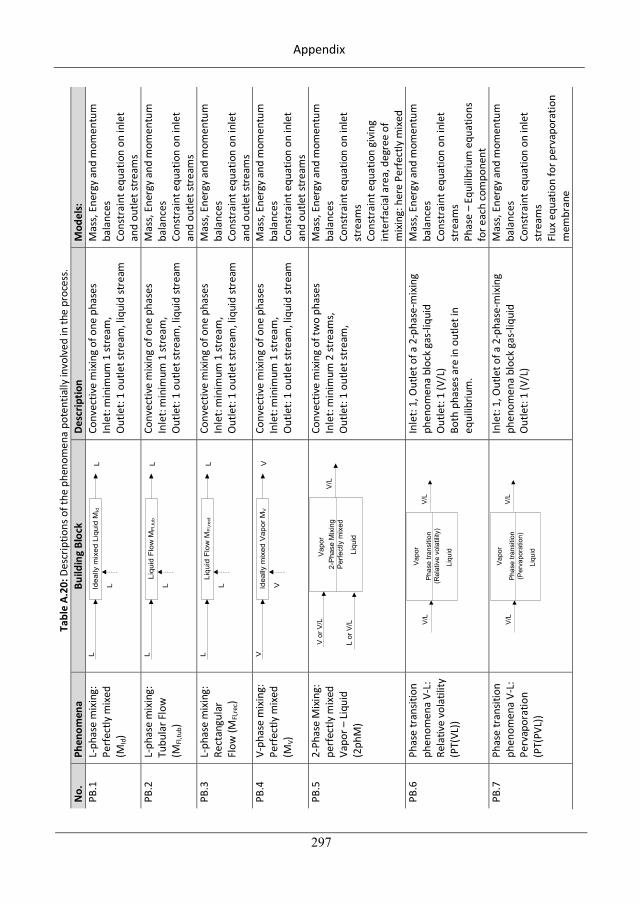
Appendix
297
Tabl
e A.
20: D
escr
iptio
ns o
f the
phe
nom
ena
pote
ntia
lly in
volv
ed in
the
proc
ess.
N
o.
Phen
omen
a Bu
ildin
g Bl
ock
Desc
riptio
n M
odel
s:
PB.1
L-
phas
e m
ixin
g:
Perf
ectly
mix
ed
(MId
)
LId
eally
mix
edLi
quid
MId
L
L
Conv
ectiv
e m
ixin
g of
one
pha
ses
Inle
t: m
inim
um 1
stre
am,
Out
let:
1 ou
tlet s
trea
m, l
iqui
d st
ream
Mas
s, En
ergy
and
mom
entu
m
bala
nces
Co
nstr
aint
equ
atio
n on
inle
t an
d ou
tlet s
trea
ms
PB.2
L-
phas
e m
ixin
g:
Tubu
lar F
low
(M
Fl,tu
b)
LLi
quid
Flo
wM
Fl,t
ubL
L
Conv
ectiv
e m
ixin
g of
one
pha
ses
Inle
t: m
inim
um 1
stre
am,
Out
let:
1 ou
tlet s
trea
m, l
iqui
d st
ream
Mas
s, En
ergy
and
mom
entu
m
bala
nces
Co
nstr
aint
equ
atio
n on
inle
t an
d ou
tlet s
trea
ms
PB.3
L-
phas
e m
ixin
g:
Rect
angu
lar
Flow
(MFl
,rec)
LLi
quid
Flo
wM
Fl,r
ect
L
L
Conv
ectiv
e m
ixin
g of
one
pha
ses
Inle
t: m
inim
um 1
stre
am,
Out
let:
1 ou
tlet s
trea
m, l
iqui
d st
ream
Mas
s, En
ergy
and
mom
entu
m
bala
nces
Co
nstr
aint
equ
atio
n on
inle
t an
d ou
tlet s
trea
ms
PB.4
V-
phas
e m
ixin
g:
Perf
ectly
mix
ed
(MV)
VId
eally
mix
edV
apor
MV
V
V
Conv
ectiv
e m
ixin
g of
one
pha
ses
Inle
t: m
inim
um 1
stre
am,
Out
let:
1 ou
tlet s
trea
m, l
iqui
d st
ream
Mas
s, En
ergy
and
mom
entu
m
bala
nces
Co
nstr
aint
equ
atio
n on
inle
t an
d ou
tlet s
trea
ms
PB.5
2-
Phas
e M
ixin
g:
perf
ectly
mix
ed
Vapo
r – L
iqui
d (2
phM
)
2-P
hase
Mix
ing
Per
fect
lym
ixed
Vap
or
Liqu
id
Vor
V/L
Lor
V/L
V/L
Conv
ectiv
e m
ixin
g of
two
phas
es
Inle
t: m
inim
um 2
stre
ams,
Out
let:
1 ou
tlet s
trea
m,
Mas
s, En
ergy
and
mom
entu
m
bala
nces
Co
nstr
aint
equ
atio
n on
inle
t st
ream
s Co
nstr
aint
equ
atio
n gi
ving
in
terf
acia
l are
a, d
egre
e of
m
ixin
g: h
ere
Perf
ectly
mix
ed
PB.6
Ph
ase
tran
sitio
n ph
enom
ena
V -L:
Re
lativ
e vo
latil
ity
(PT(
VL))
Pha
setra
nsiti
on(R
elat
ive
vola
tility
)
Vap
or
Liqu
id
V/L
V/L
Inle
t: 1,
Out
let o
f a 2
-pha
se-m
ixin
g ph
enom
ena
bloc
k ga
s -liq
uid
Out
let:
1 (V
/L)
Both
pha
ses a
re in
out
let i
n eq
uilib
rium
.
Mas
s, En
ergy
and
mom
entu
m
bala
nces
Co
nstr
aint
equ
atio
n on
inle
t st
ream
s Ph
ase
– Eq
uilib
rium
equ
atio
ns
for e
ach
com
pone
nt
PB.7
Ph
ase
tran
sitio
n ph
enom
ena
V-L:
Pe
rvap
orat
ion
(PT(
PVL)
)
Pha
setra
nsiti
on(P
erva
pora
tion)
Vap
or
Liqu
id
V/L
V/L
Inle
t: 1,
Out
let o
f a 2
-pha
se-m
ixin
g ph
enom
ena
bloc
k ga
s-liq
uid
Out
let:
1 (V
/L)
Mas
s, En
ergy
and
mom
entu
m
bala
nces
Co
nstr
aint
equ
atio
n on
inle
t st
ream
s Fl
ux e
quat
ion
for p
erva
pora
tion
mem
bran
e
327
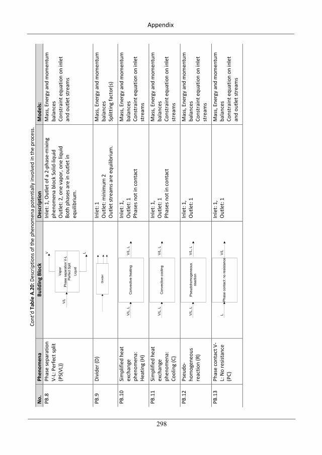
Appendix
298
Cont
’d T
able
A.2
0: D
escr
iptio
ns o
f the
phe
nom
ena
pote
ntia
lly in
volv
ed in
the
proc
ess.
No.
Ph
enom
ena
Build
ing
Bloc
k De
scrip
tion
Mod
els:
PB
.8
Phas
e se
para
tion
V-L:
Per
fect
split
(P
S(VL
)) Ph
ase
sepa
ratio
nV-
LPe
rfect
Split
Vapo
r
Liqu
id
V/L
V L
Inle
t: 1,
Out
let o
f a 2
-pha
se-m
ixin
g ph
enom
ena
bloc
k So
lid-li
quid
O
utle
t: 2,
one
vap
or, o
ne li
quid
Bo
th p
hase
s are
in o
utle
t in
equi
libriu
m.
Mas
s, En
ergy
and
mom
entu
m
bala
nces
Co
nstr
aint
equ
atio
n on
inle
t an
d ou
tlet s
trea
ms
PB.9
Di
vide
r (D)
D
ivid
er
Inle
t: 1
Out
let:
min
imum
2
Out
let s
trea
ms a
re e
quili
briu
m.
Mas
s, En
ergy
and
mom
entu
m
bala
nces
Sp
littin
g fa
ctor
(s)
PB.1
0 Si
mpl
ified
hea
t ex
chan
ge
phen
omen
a:
Heat
ing
(H)
Con
vect
ive
heat
ing
V/L
,LV
/L,L
Inle
t: 1,
O
utle
t: 1
Phas
es n
ot in
con
tact
Mas
s, En
ergy
and
mom
entu
m
bala
nces
Co
nstr
aint
equ
atio
n on
inle
t st
ream
s
PB.1
1 Si
mpl
ified
hea
t ex
chan
ge
phen
omen
a:
Cool
ing
(C)
Con
vect
ive
cool
ing
V/L
,LV
/L,L
Inle
t: 1,
O
utle
t: 1
Phas
es n
ot in
con
tact
Mas
s, En
ergy
and
mom
entu
m
bala
nces
Co
nstr
aint
equ
atio
n on
inle
t st
ream
s
PB.1
2 Ps
eudo
-ho
mog
eneo
us
reac
tion
(R)
Pse
udoh
omog
eneo
usre
actio
nV
/L,L
V/L
,L
Inle
t: 1,
O
utle
t: 1
Mas
s, En
ergy
and
mom
entu
m
bala
nces
Co
nstr
aint
equ
atio
n on
inle
t st
ream
s
PB.1
3 Ph
ase
cont
act V
-L:
No
resis
tanc
e (P
C)
Pha
seco
ntac
t:no
resi
stan
ceV
/LL
Inle
t: 1,
O
utle
t: 1
Mas
s, En
ergy
and
mom
entu
m
bala
nces
Co
nstr
aint
equ
atio
n on
inle
t an
d ou
tlet s
trea
ms
328
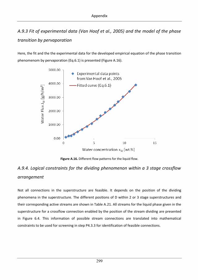
Appendix
299
A.9.3 Fit of experimental data (Van Hoof et al., 2005) and the model of the phase
transition by pervaporation
Here, the fit and the the experimental data for the developed empirical equation of the phase transition
phenomenom by pervaporation (Eq.6.1) is presented (Figure A.16).
Figure A.16. Different flow patterns for the liquid flow.
A.9.4. Logical constraints for the dividing phenomenon within a 3 stage crossflow
arrangement
Not all connections in the superstructure are feasible. It depends on the position of the dividing
phenomena in the superstructure. The different positions of D within 2 or 3 stage superstructures and
their corresponding active streams are shown in Table A.21. All streams for the liquid phase given in the
superstructure for a crossflow connection enabled by the position of the stream dividing are presented
in Figure 6.4. This information of possible stream connections are translated into mathematical
constraints to be used for screening in step P4.3.3 for identification of feasible connections.
329
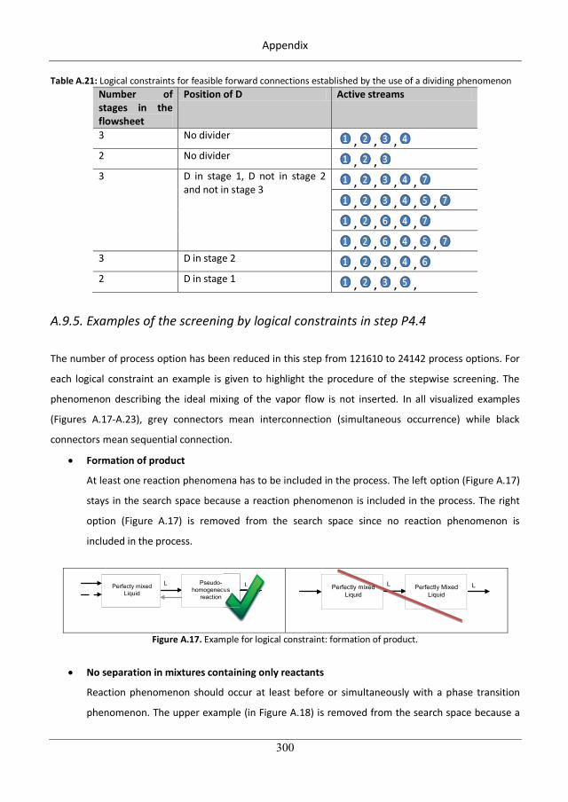
Appendix
300
Table A.21: Logical constraints for feasible forward connections established by the use of a dividing phenomenon Number of stages in the flowsheet
Position of D Active streams
3 No divider , , , 2 No divider , , 3 D in stage 1, D not in stage 2
and not in stage 3 , , , ,
, , , , ,
, , , ,
, , , , , 3 D in stage 2 , , , , 2 D in stage 1 , , , ,
A.9.5. Examples of the screening by logical constraints in step P4.4
The number of process option has been reduced in this step from 121610 to 24142 process options. For
each logical constraint an example is given to highlight the procedure of the stepwise screening. The
phenomenon describing the ideal mixing of the vapor flow is not inserted. In all visualized examples
(Figures A.17-A.23), grey connectors mean interconnection (simultaneous occurrence) while black
connectors mean sequential connection.
Formation of product
At least one reaction phenomena has to be included in the process. The left option (Figure A.17)
stays in the search space because a reaction phenomenon is included in the process. The right
option (Figure A.17) is removed from the search space since no reaction phenomenon is
included in the process.
Pseudo-homogeneous
reaction
LLPerfecty mixedLiquid ous
L
Perfectly MixedLiquid
LLPerfectly mixedLiquid
ed
Figure A.17. Example for logical constraint: formation of product.
No separation in mixtures containing only reactants
Reaction phenomenon should occur at least before or simultaneously with a phase transition
phenomenon. The upper example (in Figure A.18) is removed from the search space because a
330
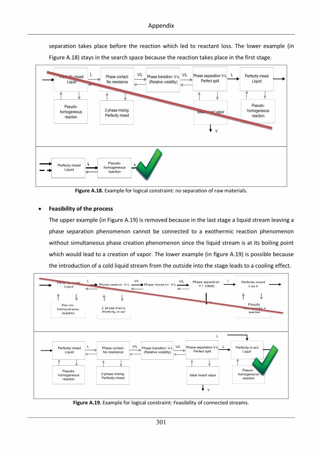
Appendix
301
separation takes place before the reaction which led to reactant loss. The lower example (in
Figure A.18) stays in the search space because the reaction takes place in the first stage.
Pseudo-homogeneous
reaction
LLPerfecty mixedLiquid
Pseudo-homogeneous
reaction
LLPerfecty mixedLiquid
LLLL
Figure A.18. Example for logical constraint: no separation of raw materials.
Feasibility of the process
The upper example (in Figure A.19) is removed because in the last stage a liquid stream leaving a
phase separation phenomenon cannot be connected to a exothermic reaction phenomenon
without simultaneous phase creation phenomenon since the liquid stream is at its boiling point
which would lead to a creation of vapor. The lower example (in figure A.19) is possible because
the introduction of a cold liquid stream from the outside into the stage leads to a cooling effect.
Phase creation: V-LLPerfectly mixed
Liquid
Pseudo-homogeneous
reaction
Phase transition: V-L
2-phase mixing:Perfectly mixed
V/L Phase separation:V-L (ideal)
Perfectly mixedLiquid
LV/L
Pseudo-homogeneous
reaction
V
Phase creation: V-LLPerfrr ectly mixed
Liquid
Pseudo-homogeneous
reaction
Phase transition: V-L
2-phase mixing:Perfrr ectly mixed
V/L Phase separation:V-L (ideal)
Perfrr ectly mixedLiquid
LV/L
Pseudo-homogeneous
reaction
V
Phase contact:No resistance
LPerfectly mixedLiquid
Pseudo-homogeneous
reaction
Phase transition: V-L(Relative volatility)
2-phase mixing:Perfectly mixed
V/L Phase separation V-LPerfect split
Perfectly mixedLiquid
LV/L
Pseudo-homogeneous
reaction
V
Ideal mixed vapor
L
mixedd
do-neousi
Figure A.19. Example for logical constraint: Feasibility of connected streams.
Phase contact:No resistance
LPerfectly mixedLiquid
Pseudo-homogeneous
reaction
Phase transition: V-L(Relative volatility)
2-phase mixing:Perfectly mixed
V/L Phase separation V-LPerfect split
Perfectly mixedLiquid
LV/L
Pseudo-homogeneous
reaction
V
Ideal mixed vapor
Perfrr ectlyid
Ideal mixed
331
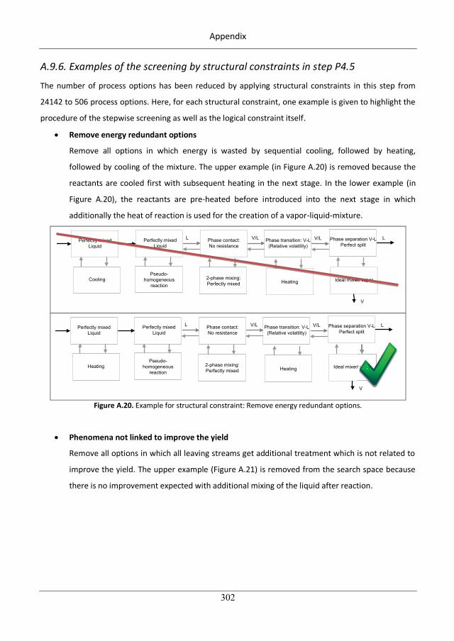
Appendix
302
A.9.6. Examples of the screening by structural constraints in step P4.5
The number of process options has been reduced by applying structural constraints in this step from
24142 to 506 process options. Here, for each structural constraint, one example is given to highlight the
procedure of the stepwise screening as well as the logical constraint itself.
Remove energy redundant options
Remove all options in which energy is wasted by sequential cooling, followed by heating,
followed by cooling of the mixture. The upper example (in Figure A.20) is removed because the
reactants are cooled first with subsequent heating in the next stage. In the lower example (in
Figure A.20), the reactants are pre-heated before introduced into the next stage in which
additionally the heat of reaction is used for the creation of a vapor-liquid-mixture.
Phase contact:No resistance
LPerfectly mixedLiquid
Pseudo-homogeneous
reaction
Phase transition: V-L(Relative volatility)
2-phase mixing:Perfectly mixed
V/L Phase separation V-LPerfect split
LV/L
V
Ideal mixed vaporHeating
Perfectly mixedLiquid
Cooling
q
l mixed vapor
P rfr ectly mixed
Phase contact:No resistance
LPerfectly mixedLiquid
Pseudo-homogeneous
reaction
Phase transition: V-L(Relative volatility)
2-phase mixing:Perfectly mixed
V/L Phase separation V-LPerfect split
LV/L
V
Ideal mixed vaporHeating
Perfectly mixedLiquid
Heating
V
d vvvvvvvvvvvvvvvvvaaaaaaaaaappoooooooooorrrrrrrrrrrrrrr
Figure A.20. Example for structural constraint: Remove energy redundant options.
Phenomena not linked to improve the yield
Remove all options in which all leaving streams get additional treatment which is not related to
improve the yield. The upper example (Figure A.21) is removed from the search space because
there is no improvement expected with additional mixing of the liquid after reaction.
332
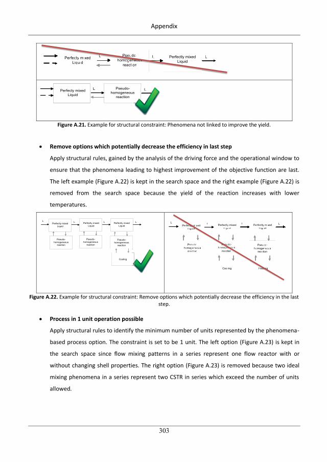
Appendix
303
Pseudo-homogeneous
reaction
LLPerfecty mixedLiquid Cooling
LPseudo-homogeneous
reaction
LLPerfr ecty mixedLiquid Cooling
LPerfectly mixedLiquid
Pseudo-homogeneous
reaction
LLPerfecty mixedLiquid s
L
Figure A.21. Example for structural constraint: Phenomena not linked to improve the yield.
Remove options which potentially decrease the efficiency in last step
Apply structural rules, gained by the analysis of the driving force and the operational window to
ensure that the phenomena leading to highest improvement of the objective function are last.
The left example (Figure A.22) is kept in the search space and the right example (Figure A.22) is
removed from the search space because the yield of the reaction increases with lower
temperatures.
Perfectly mixedLiquid
LPerfectly mixedLiquid
Pseudo-homogeneous
reaction
Pseudo-homogeneous
reaction
LPerfectly mixedLiquid
Pseudo-homogeneous
reaction
L L
Cooling
Perfectly mixedLiquid
LPerfectly mixedLiquid
Pseudo-homogeneous
reaction
Pseudo-homogeneous
reaction
LPerfectly mixedLiquid
Pseudo-homogeneous
reaction
L L
Cooling Heating
Perfr ectly mixedLiquid
LPerfrr ectly mixedLiquid
Pseudo-homogeneous
reaction
Pseudo-homogeneous
reaction
LPerfrr ectly mixedLiquid
Pseudo-homogeneous
reaction
L L
Cooling Heating
Figure A.22. Example for structural constraint: Remove options which potentially decrease the efficiency in the last
step.
Process in 1 unit operation possible
Apply structural rules to identify the minimum number of units represented by the phenomena-
based process option. The constraint is set to be 1 unit. The left option (Figure A.23) is kept in
the search space since flow mixing patterns in a series represent one flow reactor with or
without changing shell properties. The right option (Figure A.23) is removed because two ideal
mixing phenomena in a series represent two CSTR in series which exceed the number of units
allowed.
333
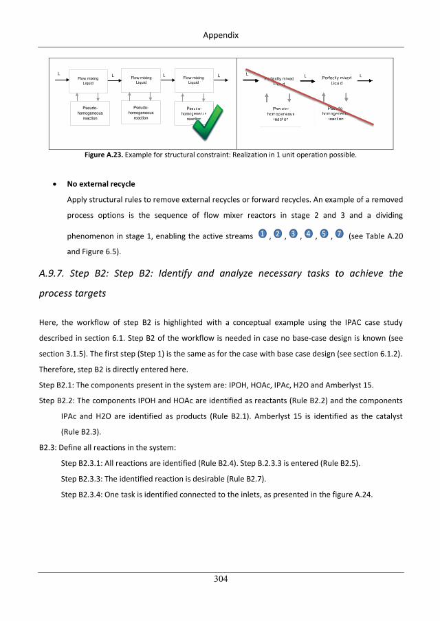
Appendix
304
Perfectly mixedLiquid
LPerfectly mixedLiquid
Pseudo-homogeneous
reaction
Pseudo-homogeneous
reaction
LPerfectly mixedLiquid
Pseudo-homogeneous
reaction
L L
seudo-ogeneousactiioooooooooooooooon
Flow mixingLiquid
Flow mixingLiquid
Flow mixingLiquid
LPerfectly mixedLiquid
Pseudo-homogeneous
reaction
Perfectly mixedLiquid
Pseudo-homogeneous
reaction
L L LPerfrr ectly mixedLiquid
Pseudo-homogeneous
reaction
Perfrr ectly mixedLiquid
Pseudo-homogeneous
reaction
L L
Figure A.23. Example for structural constraint: Realization in 1 unit operation possible.
No external recycle
Apply structural rules to remove external recycles or forward recycles. An example of a removed
process options is the sequence of flow mixer reactors in stage 2 and 3 and a dividing
phenomenon in stage 1, enabling the active streams , , , , , (see Table A.20
and Figure 6.5).
A.9.7. Step B2: Step B2: Identify and analyze necessary tasks to achieve the
process targets
Here, the workflow of step B2 is highlighted with a conceptual example using the IPAC case study
described in section 6.1. Step B2 of the workflow is needed in case no base-case design is known (see
section 3.1.5). The first step (Step 1) is the same as for the case with base case design (see section 6.1.2).
Therefore, step B2 is directly entered here.
Step B2.1: The components present in the system are: IPOH, HOAc, IPAc, H2O and Amberlyst 15.
Step B2.2: The components IPOH and HOAc are identified as reactants (Rule B2.2) and the components
IPAc and H2O are identified as products (Rule B2.1). Amberlyst 15 is identified as the catalyst
(Rule B2.3).
B2.3: Define all reactions in the system:
Step B2.3.1: All reactions are identified (Rule B2.4). Step B.2.3.3 is entered (Rule B2.5).
Step B2.3.3: The identified reaction is desirable (Rule B2.7).
Step B2.3.4: One task is identified connected to the inlets, as presented in the figure A.24.
334
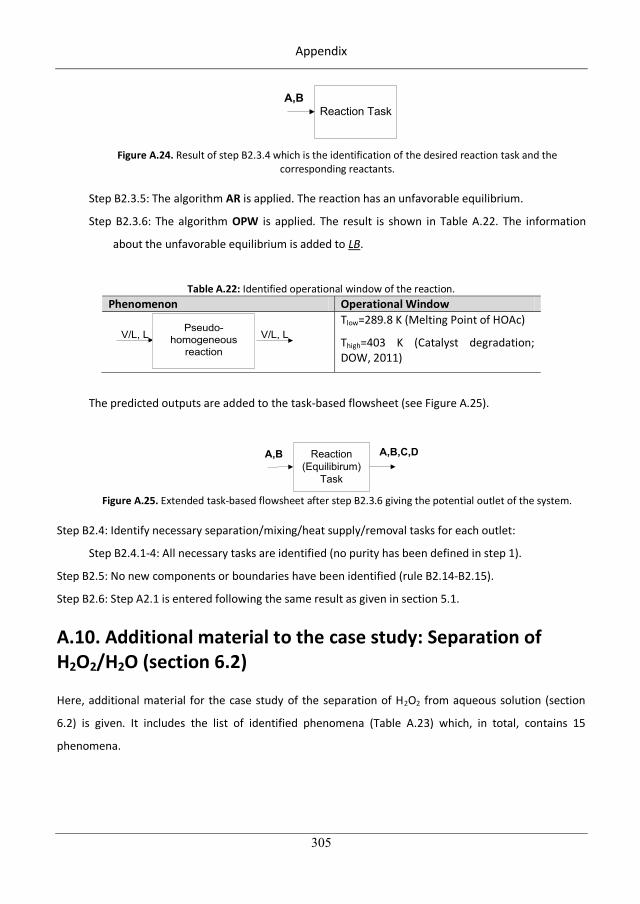
Appendix
305
Reaction TaskA,B
Figure A.24. Result of step B2.3.4 which is the identification of the desired reaction task and the
corresponding reactants.
Step B2.3.5: The algorithm AR is applied. The reaction has an unfavorable equilibrium.
Step B2.3.6: The algorithm OPW is applied. The result is shown in Table A.22. The information
about the unfavorable equilibrium is added to LB.
Table A.22: Identified operational window of the reaction. Phenomenon Operational Window
Pseudo-homogeneous
reaction
V/L, LV/L, L
Tlow=289.8 K (Melting Point of HOAc)
Thigh=403 K (Catalyst degradation; DOW, 2011)
The predicted outputs are added to the task-based flowsheet (see Figure A.25).
Reaction(Equilibirum)
Task
A,B A,B,C,D
Figure A.25. Extended task-based flowsheet after step B2.3.6 giving the potential outlet of the system.
Step B2.4: Identify necessary separation/mixing/heat supply/removal tasks for each outlet:
Step B2.4.1-4: All necessary tasks are identified (no purity has been defined in step 1).
Step B2.5: No new components or boundaries have been identified (rule B2.14-B2.15).
Step B2.6: Step A2.1 is entered following the same result as given in section 5.1.
A.10. Additional material to the case study: Separation of H2O2/H2O (section 6.2)
Here, additional material for the case study of the separation of H2O2 from aqueous solution (section
6.2) is given. It includes the list of identified phenomena (Table A.23) which, in total, contains 15
phenomena.
335
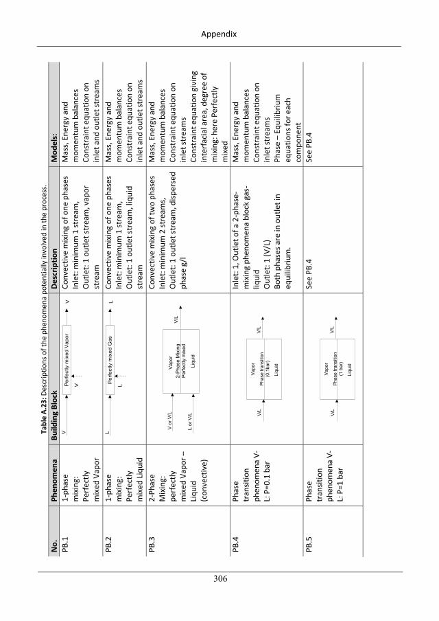
Appendix
306
Tabl
e A.
23: D
escr
iptio
ns o
f the
phe
nom
ena
pote
ntia
lly in
volv
ed in
the
proc
ess.
N
o.
Phen
omen
a Bu
ildin
g Bl
ock
Desc
riptio
n M
odel
s:
PB.1
1-
phas
e m
ixin
g:
Perf
ectly
m
ixed
Vap
or
VP
erfe
ctly
mix
edV
apor
V
V
Conv
ectiv
e m
ixin
g of
one
pha
ses
Inle
t: m
inim
um 1
stre
am,
Out
let:
1 ou
tlet s
trea
m, v
apor
st
ream
Mas
s, En
ergy
and
m
omen
tum
bal
ance
s Co
nstr
aint
equ
atio
n on
in
let a
nd o
utle
t str
eam
s PB
.2
1-ph
ase
mix
ing:
Pe
rfec
tly
mix
ed Li
quid
LP
erfe
ctly
mix
edG
asL
L
Conv
ectiv
e m
ixin
g of
one
pha
ses
Inle
t: m
inim
um 1
stre
am,
Out
let:
1 ou
tlet s
trea
m, l
iqui
d st
ream
Mas
s, En
ergy
and
m
omen
tum
bal
ance
s Co
nstr
aint
equ
atio
n on
in
let a
nd o
utle
t str
eam
s PB
.3
2-Ph
ase
Mix
ing:
pe
rfec
tly
mix
ed V
apor
–
Liqu
id
(con
vect
ive)
2-P
hase
Mix
ing
Per
fect
lym
ixed
Vap
or
Liqu
id
Vor
V/L
Lor
V/L
V/L
Conv
ectiv
e m
ixin
g of
two
phas
es
Inle
t: m
inim
um 2
stre
ams,
O
utle
t: 1
outle
t str
eam
, disp
erse
d ph
ase
g/l
Mas
s, En
ergy
and
m
omen
tum
bal
ance
s Co
nstr
aint
equ
atio
n on
in
let s
trea
ms
Cons
trai
nt e
quat
ion
givi
ng
inte
rfac
ial a
rea,
deg
ree
of
mix
ing:
her
e Pe
rfec
tly
mix
ed
PB.4
Ph
ase
tran
sitio
n ph
enom
ena
V-L:
P=0
.1 b
ar
Phas
etra
nsiti
on(0
.1ba
r)
Vapo
r
Liqu
id
V/L
V/L
Inle
t: 1,
Out
let o
f a 2
-pha
se-
mix
ing
phen
omen
a bl
ock
gas -
liqui
d O
utle
t: 1
(V/L
) Bo
th p
hase
s are
in o
utle
t in
equi
libriu
m.
Mas
s, En
ergy
and
m
omen
tum
bal
ance
s Co
nstr
aint
equ
atio
n on
in
let s
trea
ms
Phas
e –
Equi
libriu
m
equa
tions
for e
ach
com
pone
nt
PB.5
Ph
ase
tran
sitio
n ph
enom
ena
V-L:
P=1
bar
Phas
etra
nsiti
on(1
bar)
Vapo
r
Liqu
id
V/L
V/L
See
PB.4
Se
e PB
.4
336
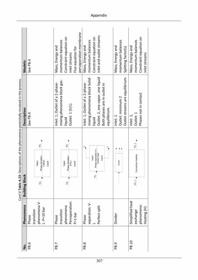
Appendix
307
Cont
’d T
able
A.2
3: D
escr
iptio
ns o
f the
phe
nom
ena
pote
ntia
lly in
volv
ed in
the
proc
ess.
N
o.
Phen
omen
a Bu
ildin
g Bl
ock
Desc
riptio
n M
odel
s:
PB.6
Ph
ase
tran
sitio
n ph
enom
ena
V-L:
P=1
0 ba
r
Phas
etra
nsiti
on(1
0bar
)
Vapo
r
Liqu
id
V/L
V/L
See
PB.4
Se
e PB
.4
PB.7
Ph
ase
tran
sitio
n ph
enom
ena
Perv
apor
atio
n:
P=1
bar
Phas
etra
nsiti
on(P
VL)
Vapo
r
Liqu
id
V/L
V/L
Inle
t: 1,
Out
let o
f a 2
-pha
se-
mix
ing
phen
omen
a bl
ock
gas-
liqui
d O
utle
t: 1
(V/L
)
Mas
s, En
ergy
and
m
omen
tum
bal
ance
s Co
nstr
aint
equ
atio
n on
in
let s
trea
ms
Flux
equ
atio
n fo
r pe
rvap
orat
ion
mem
bran
e PB
.8
Phas
e se
para
tion:
V-
L Perf
ect s
plit
Phas
ese
para
tion
V-L
Perfe
ctSp
lit
Vapo
r
Liqu
id
V/L
V L
Inle
t: 1,
Out
let o
f a 2
-pha
se-
mix
ing
phen
omen
a bl
ock
Solid
-liq
uid
Out
let:
2, o
ne v
apor
, one
liqu
id
Both
pha
ses a
re in
out
let i
n eq
uilib
rium
.
Mas
s, En
ergy
and
m
omen
tum
bal
ance
s Co
nstr
aint
equ
atio
n on
in
let a
nd o
utle
t str
eam
s
PB.9
Di
vide
r D
ivid
er
Inle
t: 1
Out
let:
min
imum
2
Out
let s
trea
ms a
re e
quili
briu
m.
Mas
s, En
ergy
and
m
omen
tum
bal
ance
s Sp
littin
g fa
ctor
(s)
PB.1
0 Si
mpl
ified
hea
t ex
chan
ge
phen
omen
a:
Heat
ing
(H)
Con
vect
ive
heat
ing
V/L
,LV
/L,L
Inle
t: 1,
O
utle
t: 1
Phas
es n
ot in
cont
act
Mas
s, En
ergy
and
m
omen
tum
bal
ance
s Co
nstr
aint
equ
atio
n on
in
let s
trea
ms
337
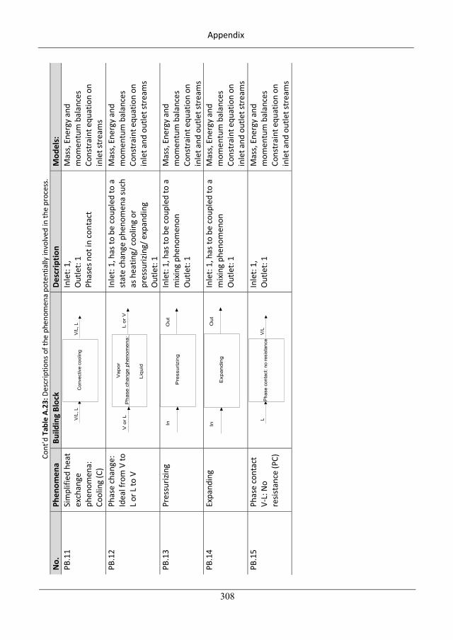
Appendix
308
Cont
’d T
able
A.2
3: D
escr
iptio
ns o
f the
phe
nom
ena
pote
ntia
lly in
volv
ed in
the
proc
ess.
N
o.
Phen
omen
a Bu
ildin
g Bl
ock
Desc
riptio
n M
odel
s:
PB.1
1 Si
mpl
ified
hea
t ex
chan
ge
phen
omen
a:
Cool
ing
(C)
Con
vect
ive
cool
ing
V/L
,LV
/L,L
Inle
t: 1,
O
utle
t: 1
Phas
es n
ot in
cont
act
Mas
s, En
ergy
and
m
omen
tum
bal
ance
s Co
nstr
aint
equ
atio
n on
in
let s
trea
ms
PB.1
2 Ph
ase
chan
ge:
Idea
l fro
m V
to
L or L
to V
P
hase
chan
geph
enom
ena:
Vap
or
Liqu
id
Vor
LL
orV
Inle
t: 1,
has
to b
e co
uple
d to
a
stat
e ch
ange
phe
nom
ena
such
as
hea
ting/
cool
ing
or
pres
suriz
ing/
exp
andi
ng
Out
let:
1
Mas
s, En
ergy
and
m
omen
tum
bal
ance
s Co
nstr
aint
equ
atio
n on
in
let a
nd o
utle
t str
eam
s
PB.1
3 Pr
essu
rizin
g In
Out
Pre
ssur
izin
g
Inle
t: 1,
has
to b
e co
uple
d to
a
mix
ing
phen
omen
on
Out
let:
1
Mas
s, En
ergy
and
m
omen
tum
bal
ance
s Co
nstr
aint
equ
atio
n on
in
let a
nd o
utle
t str
eam
s PB
.14
Expa
ndin
g In
Out
Exp
andi
ng
Inle
t: 1,
has
to b
e co
uple
d to
a
mix
ing
phen
omen
on
Out
let:
1
Mas
s, En
ergy
and
m
omen
tum
bal
ance
s Co
nstr
aint
equ
atio
n on
in
let a
nd o
utle
t str
eam
s PB
.15
Phas
e co
ntac
t V-
L: N
o re
sista
nce
(PC)
P
hase
cont
act:
nore
sist
ance
V/L
L
Inle
t: 1,
O
utle
t: 1
Mas
s, En
ergy
and
m
omen
tum
bal
ance
s Co
nstr
aint
equ
atio
n on
in
let a
nd o
utle
t str
eam
s
338
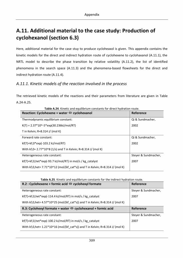
Appendix
309
A.11. Additional material to the case study: Production of cyclohexanol (section 6.3)
Here, additional material for the case stuy to produce cycloheaxol is given. This appendix contains the
kinetic models for the direct and indirect hydration route of cyclohexene to cyclohaxanol (A.11.1), the
NRTL model to describe the phase transition by relative volatility (A.11.2), the list of identified
phenomena in the search space (A.11.3) and the phenomena-based flowsheets for the direct and
indirect hydration route (A.11.4).
A.11.1. Kinetic models of the reaction involved in the process
The retrieved kinetic models of the reactions and their parameters from literature are given in Table
A.24-A.25.
Table A.24. Kinetic and equilibrium constants for direct hydration route. Reaction: Cyclohexene + water cyclohexanol Reference
Thermodynamic equilibrium constant:
K(T) = 2.37*10^-5*exp(30.236kJ/mol/RT)
T in Kelvin; R=8.314 J/ (mol K)
Qi & Sundmacher,
2002
Forward rate constant:
kf(T)=kf,0*exp(-103.2 kJ/mol/RT)
With kf,0= 2.77*10^8 (1/s) and T in Kelvin; R=8.314 J/ (mol K)
Qi & Sundmacher,
2002
Heterogeneous rate constant:
kf(T)=kf,0,het*exp(-93.7 kJ/mol/RT) in mol/s / kg_catalyst
With kf,0,het= 7.71*10^12 (mol/(kf_cat*s)) and T in Kelvin; R=8.314 J/ (mol K)
Steyer & Sundmacher,
2007
Table A.25. Kinetic and equilibrium constants for the indirect hydration route. R.2 : Cyclohexene + formic acid cyclohexyl formate Reference
Heterogeneous rate constant:
kf(T)=kf,0,het*exp(-114.4 kJ/mol/RT) in mol/s / kg_catalyst
With kf,0,het= 4.57*10^25 (mol/(kf_cat*s)) and T in Kelvin; R=8.314 J/ (mol K)
Steyer & Sundmacher,
2007
R.3: Cyclohexyl formate + water cyclohexanol + formic acid Reference
Heterogeneous rate constant:
kf(T)=kf,0,het*exp(-100.2 kJ/mol/RT) in mol/s / kg_catalyst
With kf,0,het= 1.21*10^16 (mol/(kf_cat*s)) and T in Kelvin; R=8.314 J/ (mol K)
Steyer & Sundmacher,
2007
339
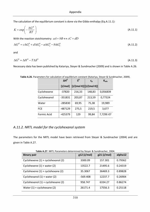
Appendix
310
The calculation of the equilibrium constant is done via the Gibbs-enthalpy (Eq.A.11.1):
expRGK
RT (A.11.1)
With the reaction stoichiometry: aA bB cC dD 0 0 0 0Rc d a bG c G d G a G b G (A.11.2)
and
0 0 0G H T S (A.11.3)
Necessary data has been published by Katariya, Steyer & Sundmacher (2009) and is shown in Table A.26.
Table A.26. Parameters for calculation of equilibrium constant (Katariya, Steyer & Sundmacher, 2009). H0 S0 cp Kads
[J/mol] [J/(mol K)] [J/(mol K)]
Cyclohexene -37820 216,33 148,83 0,056839
Cyclohexanol -351831 203,87 213,59 0,77324
Water -285830 69,95 75,38 19,989
FCE -487129 275,5 219,5 3,677
Formic Acid -425379 129 99,84 7,729E-07
A.11.2. NRTL model for the cyclohexanol system
The parameters for the NRTL model have been retrieved from Steyer & Sundmacher (2004) and are
given in Table A.27.
Table A.27. NRTL Parameters determined by Steyer & Sundmacher, 2004.
Binary pair g12 (J/mol) g21 (J/mol) alpha12
Cyclohexene (1) + cyclohexanol (2) 3300.09 157.301 0.79362
Cyclohexene (1) + water (2) 13522.7 21495.6 0.24319
Cyclohexene (1) + cyclohexane (2) 35.3067 36469.3 0.89828
Cyclohexanol (1) + water (2) -569.408 12237.7 0.26904
Cyclohexanol (1) + cyclohexane (2) 958.747 6334.27 0.86274
Water (1) + cyclohexane (2) 26171.4 17556.3 0.25118
340
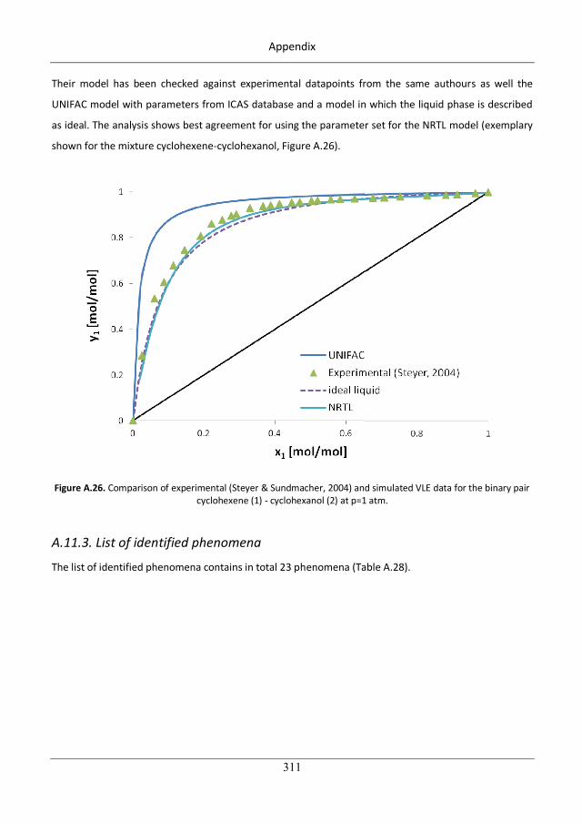
Appendix
311
Their model has been checked against experimental datapoints from the same authours as well the
UNIFAC model with parameters from ICAS database and a model in which the liquid phase is described
as ideal. The analysis shows best agreement for using the parameter set for the NRTL model (exemplary
shown for the mixture cyclohexene-cyclohexanol, Figure A.26).
Figure A.26. Comparison of experimental (Steyer & Sundmacher, 2004) and simulated VLE data for the binary pair cyclohexene (1) - cyclohexanol (2) at p=1 atm.
A.11.3. List of identified phenomena
The list of identified phenomena contains in total 23 phenomena (Table A.28).
341
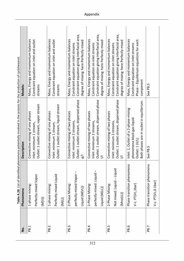
Appendix
312
Tabl
e A.
28. L
ist o
f ide
ntifi
ed p
heno
men
a po
tent
ially
invo
lved
in th
e pr
oces
s for
the
prod
uctio
n of
cyc
lohe
xano
l. N
o.
Phen
omen
a De
scrip
tion
Mod
els:
PB.1
1-
phas
e m
ixin
g:
Perf
ectly
mix
ed V
apor
(M(V
))
Conv
ectiv
e m
ixin
g of
one
pha
ses
Inle
t: m
inim
um 1
stre
am,
Out
let:
1 ou
tlet s
trea
m, v
apor
stre
am
Mas
s, En
ergy
and
mom
entu
m b
alan
ces
Cons
trai
nt e
quat
ion
on in
let a
nd o
utle
t st
ream
s
PB.2
1-
phas
e m
ixin
g:
Perf
ectly
mix
ed Li
quid
(M(L
))
Conv
ectiv
e m
ixin
g of
one
pha
ses
Inle
t: m
inim
um 1
stre
am,
Out
let:
1 ou
tlet s
trea
m, l
iqui
d st
ream
Mas
s, En
ergy
and
mom
entu
m b
alan
ces
Cons
trai
nt e
quat
ion
on in
let a
nd o
utle
t st
ream
s
PB.3
2-
Phas
e M
ixin
g:
perf
ectly
mix
ed V
apor
–
Liqu
id (M
(VL)
)
Conv
ectiv
e m
ixin
g of
two
phas
es
Inle
t: m
inim
um 2
stre
ams,
O
utle
t: 1
outle
t str
eam
, disp
erse
d ph
ase
g/l
Mas
s, En
ergy
and
mom
entu
m b
alan
ces
Cons
trai
nt e
quat
ion
on in
let s
trea
ms
Cons
trai
nt e
quat
ion
givi
ng in
terf
acia
l are
a,
degr
ee o
f mix
ing:
her
e Pe
rfec
tly m
ixed
PB.4
2-
Phas
e M
ixin
g:
perf
ectly
mix
ed: L
i qui
d –
Liqu
id (M
(LL)
)
Conv
ectiv
e m
ixin
g of
two
phas
es
Inle
t: m
inim
um 2
stre
ams,
O
utle
t: 1
outle
t str
eam
, disp
erse
d ph
ase
l/l
Mas
s, En
ergy
and
mom
entu
m b
alan
ces
Cons
trai
nt e
quat
ion
on in
let s
trea
ms
Cons
trai
nt e
quat
ion
givi
ng in
terf
acia
l are
a,
degr
ee o
f mix
i ng:
her
e Pe
rfec
tly m
ixed
PB.5
2-
Phas
e M
ixin
g:
Not
mix
ed: L
iqui
d –
Liqu
id
(Mno
(LL)
)
Conv
ectiv
e m
ixin
g of
two
phas
es
Inle
t: m
inim
um 2
stre
ams,
O
utle
t: 1
outle
t str
eam
, disp
erse
d ph
ase
l/l
Mas
s, En
ergy
and
mom
entu
m b
alan
ces
Cons
trai
nt e
quat
ion
on in
let s
trea
ms
Cons
trai
nt e
quat
ion
givi
ng in
terf
acia
l are
a,
degr
ee o
f mix
ing:
her
e Pe
rfec
tly m
ixed
PB.6
Ph
ase
tran
sitio
n ph
enom
ena
V-L:
PT(
VL,1
bar)
Inle
t: 1,
Out
let o
f a 2
-pha
se-m
ixin
g ph
enom
ena
bloc
k ga
s-liq
uid
Out
let:
1 (V
/L)
Both
pha
ses a
re in
out
let i
n eq
uilib
rium
.
Mas
s, En
ergy
and
mom
entu
m b
alan
ces
Cons
trai
nt e
quat
ion
on in
let s
trea
ms
Phas
e –
Equi
libriu
m e
quat
ions
for e
ach
com
pone
nt
PB.7
Ph
ase
tran
sitio
n ph
enom
ena
V-L:
PT(
VL,0
.1ba
r)
See
PB.5
Se
e PB
.5
342
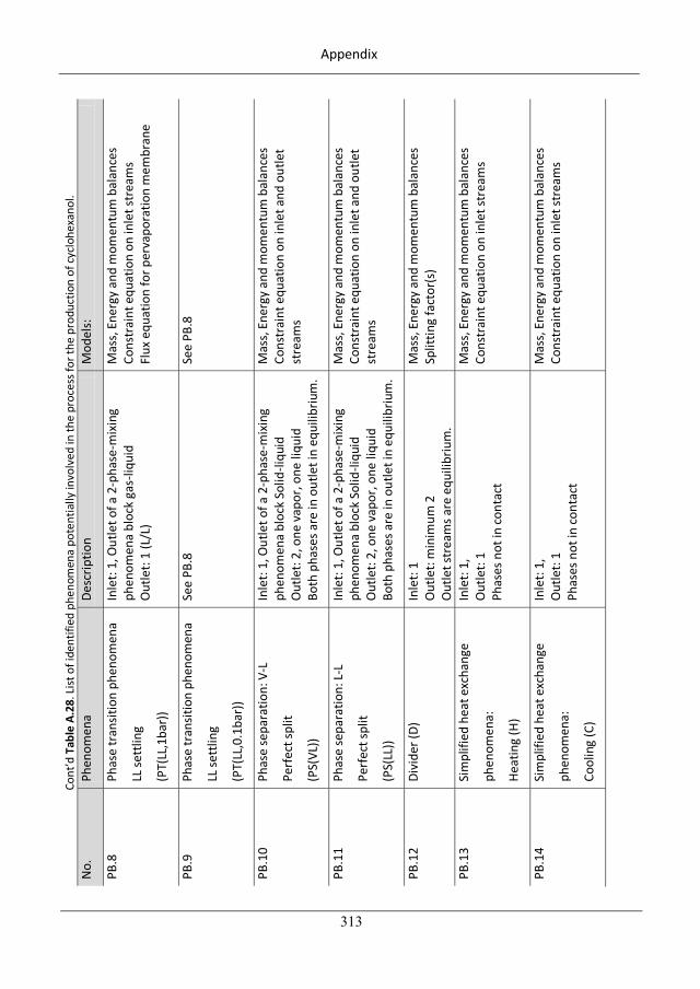
Appendix
313
Cont
’d T
able
A.2
8. L
ist o
f ide
ntifi
ed p
heno
men
a po
tent
ially
invo
lved
in th
e pr
oces
s for
the
prod
uctio
n of
cyc
lohe
xano
l. N
o.
Phen
omen
a De
scrip
tion
Mod
els:
PB.8
Ph
ase
tran
sitio
n ph
enom
ena
LL se
ttlin
g
(PT(
LL,1
bar)
)
Inle
t: 1,
Out
let o
f a 2
-pha
se-m
ixin
g ph
enom
ena
bloc
k ga
s-liq
uid
Out
let:
1 (L
/L)
Mas
s, En
ergy
and
mom
entu
m b
alan
ces
Cons
trai
nt e
quat
ion
on in
let s
trea
ms
Flux
equ
atio
n fo
r per
vapo
ratio
n m
embr
ane
PB.9
Ph
ase
tran
sitio
n ph
enom
ena
LL se
ttlin
g
(PT(
LL,0
.1ba
r))
See
PB.8
Se
e PB
.8
PB.1
0 Ph
ase
sepa
ratio
n: V
-L
Perf
ect s
plit
(PS(
VL))
Inle
t: 1,
Out
let o
f a 2
-pha
se-m
ixin
g ph
enom
ena
bloc
k So
lid-li
quid
O
utle
t: 2,
one
vap
or, o
ne li
quid
Bo
th p
hase
s are
in o
utle
t in
equi
libriu
m.
Mas
s, En
ergy
and
mom
entu
m b
alan
ces
Cons
trai
nt e
quat
ion
on in
let a
nd o
utle
t st
ream
s
PB.1
1 Ph
ase
sepa
ratio
n: L
-L
Perf
ect s
plit
(PS(
LL))
Inle
t: 1,
Out
let o
f a 2
-pha
se-m
ixin
g ph
enom
ena
bloc
k So
lid-li
quid
O
utle
t: 2,
one
vap
or, o
ne li
quid
Bo
th p
hase
s are
in o
utle
t in
equi
libriu
m.
Mas
s, En
ergy
and
mom
entu
m b
alan
ces
Cons
trai
nt e
quat
ion
on in
let a
nd o
utle
t st
ream
s
PB.1
2 Di
vide
r (D)
In
let:
1 O
utle
t: m
inim
um 2
O
utle
t str
eam
s are
equ
ilibr
ium
.
Mas
s, En
ergy
and
mom
entu
m b
alan
ces
Split
ting
fact
or(s
)
PB.1
3 Si
mpl
ified
hea
t exc
hang
e
phen
omen
a:
Heat
ing
(H)
Inle
t: 1,
O
utle
t: 1
Phas
es n
ot in
cont
act
Mas
s, En
ergy
and
mom
entu
m b
alan
ces
Cons
trai
nt e
quat
ion
on in
let s
trea
ms
PB.1
4 Si
mpl
ified
hea
t exc
hang
e
phen
omen
a:
Cool
ing
(C)
Inle
t: 1,
O
utle
t: 1
Phas
es n
ot in
cont
act
Mas
s, En
ergy
and
mom
entu
m b
alan
ces
Cons
trai
nt e
quat
ion
on in
let s
trea
ms
343
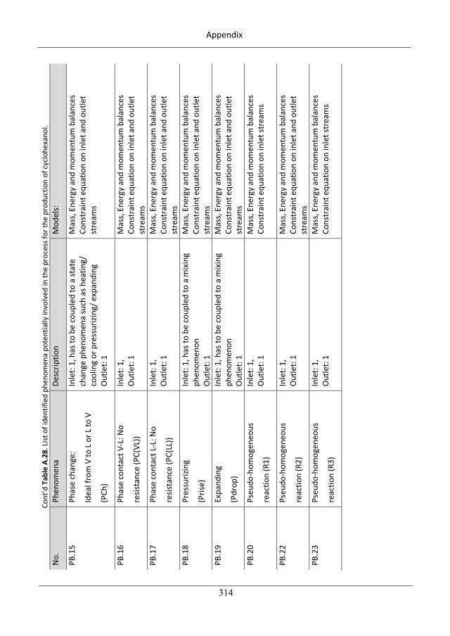
Appendix
314
Cont
’d T
able
A.2
8. L
ist o
f ide
ntifi
ed p
heno
men
a po
tent
ially
invo
lved
in th
e pr
oces
s for
the
prod
uctio
n of
cyc
lohe
xano
l. N
o.
Phen
omen
a De
scrip
tion
Mod
els:
PB.1
5 Ph
ase
chan
ge:
Idea
l fro
m V
to L
or L
to V
(PCh
)
Inle
t: 1,
has
to b
e co
uple
d to
a st
ate
chan
ge p
heno
men
a su
ch a
s hea
ting/
co
olin
g or
pre
ssur
izing
/ exp
andi
ng
Out
let:
1
Mas
s, En
ergy
and
mom
entu
m b
alan
ces
Cons
trai
nt e
quat
ion
on in
let a
nd o
utle
t st
ream
s
PB.1
6 Ph
ase
cont
act V
-L: N
o
resis
tanc
e (P
C(VL
))
Inle
t: 1,
O
utle
t: 1
Mas
s, En
ergy
and
mom
entu
m b
alan
ces
Cons
trai
nt e
quat
ion
on in
let a
nd o
utle
t st
ream
s PB
.17
Phas
e co
ntac
t L-L
: No
resis
tanc
e (P
C(LL
))
Inle
t: 1,
O
utle
t: 1
Mas
s, En
ergy
and
mom
entu
m b
alan
ces
Cons
trai
nt e
quat
ion
on in
let a
nd o
utle
t st
ream
s PB
.18
Pres
suriz
ing
(Pris
e)
Inle
t: 1,
has
to b
e co
uple
d to
a m
ixin
g ph
enom
enon
O
utle
t: 1
Mas
s, En
ergy
and
mom
entu
m b
alan
ces
Cons
trai
nt e
quat
ion
on in
let a
nd o
utle
t st
ream
s PB
.19
Expa
ndin
g
(Pdr
op)
Inle
t: 1,
has
to b
e co
uple
d to
a m
ixin
g ph
enom
enon
O
utle
t: 1
Mas
s, En
ergy
and
mom
entu
m b
alan
ces
Cons
trai
nt e
quat
ion
on in
let a
nd o
utle
t st
ream
s PB
.20
Pseu
do-h
omog
eneo
us
reac
tion
(R1)
Inle
t: 1,
O
utle
t: 1
Mas
s, En
ergy
and
mom
entu
m b
alan
ces
Cons
trai
nt e
quat
ion
on in
let s
trea
ms
PB.2
2 Ps
eudo
-hom
ogen
eous
reac
tion
(R2)
Inle
t: 1,
O
utle
t: 1
Mas
s, En
ergy
and
mom
entu
m b
alan
ces
Cons
trai
nt e
quat
ion
on in
let a
nd o
utle
t st
ream
s PB
.23
Pseu
do-h
omog
eneo
us
reac
tion
(R3)
Inle
t: 1,
O
utle
t: 1
Mas
s, En
ergy
and
mom
entu
m b
alan
ces
Cons
trai
nt e
quat
ion
on in
let s
trea
ms
344
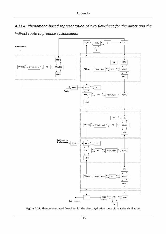
Appendix
315
A.11.4. Phenomena-based representation of two flowsheet for the direct and the
indirect route to produce cyclohexanol
Figure A.27. Phenomena-based flowsheet for the direct hydration route via reactive distillation.
345
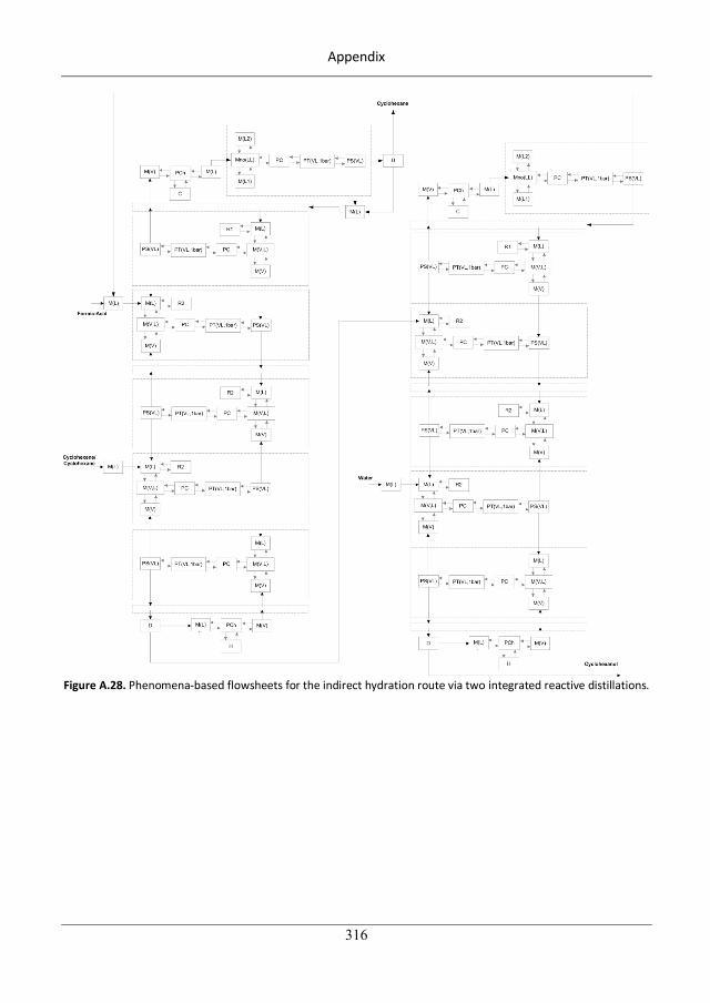
Appendix
316
Figure A.28. Phenomena-based flowsheets for the indirect hydration route via two integrated reactive distillations.
346

Center for Process Engineering and Technology (PROCESS)
Department of Chemical and Biochemical Engineering
Technical University of Denmark
Søltofts Plads, Building 229
DK-2800 Kgs. Lyngby
Denmark
Phone: +45 4525 2800
Fax: +45 4525 2906
Web: www.process.kt.dtu.dk
ISBN : 978-87-92481-67-2


![AN INNOVATIVE METHODOLOGY FOR ERROR ANALYSIS … · AN INNOVATIVE METHODOLOGY FOR ERROR ANALYSIS OF ... creation of Computational Fluid Dynamics ... Hoffmann Nozzle [4]](https://img.pdfslide.net/doc/110x75/5b1bf7847f8b9a2d258f1cc1/an-innovative-methodology-for-error-analysis-an-innovative-methodology-for-error.jpg)