�������������������������� �������������������������������������������������������

������������������������������������

��������������������������������������������

������ �� ��� ���� ����� ��������� ����� �������� ���� ��� � ��� ���� ��������

���������������� �������������������������������������������������

������ ��������������������

����������������� �

��������������

an author's http://oatao.univ-toulouse.fr/21867

https://www.kybernetika.cz/content/2018/1/202

Brunot, Mathieu and Janot, Alexandre and Young, Peter C. and Carrillo, Francisco Javier An instrumental variable

method for robot identification based on time variable parameter estimation. (2018) KYBERNETIKA, 54 (1). 202-220.

ISSN 0023-5954

AN INSTRUMENTAL VARIABLE METHOD

FOR ROBOT IDENTIFICATION BASED ON

TIME VARIABLE PARAMETER ESTIMATION

Mathieu Brunot, Alexandre Janot, Peter C. Young

and Francisco Carrillo

This paper considers the data-based identification of industrial robots using an instrumentalvariable method that uses off-line estimation of the joint velocities and acceleration signalsbased only on the measurement of the joint positions. The usual approach to this problemrelies on a ‘tailor-made’ prefiltering procedure for estimating the derivatives that depends ongood prior knowledge of the system’s bandwidth. The paper describes an alternative IntegratedRandom Walk SMoothing (IRWSM) method that is more robust to deficiencies in such a prioriknowledge and exploits an optimal recursive algorithm based on a simple integrated randomwalk model and a Kalman filter with associated fixed interval smoothing. The resultant IDIM-IV instrumental variable method, using this approach to signal generation, is evaluated by itsapplication to an industrial robot arm and comparison with previously proposed methods.

Keywords: industrial robot system, system identification, instrumental variable method,parameter estimation, Kalman filter, fixed interval smoothing

1. INTRODUCTION

For many years, the most common method used for robot identification has been basedon Least-Squares (LS) optimization and estimation of the Inverse Dynamic IdentificationModel (IDIM): see e. g. [9] or [10]. The IDIM expresses the input torque as a linearfunction of the physical parameters thanks to the modified Denavit and Hartenberg(DHM) notation: see e. g. [15]. Although this is a popular and quite successful method,it is not always robust to the measurement noise correlation that arises from the closed-loop structure required for robot operation.

In order to avoid possible bias in the model parameter estimates, an InstrumentalVariable (IV) method has been been suggested and successfully evaluated on robotsystems [14]. Like the IDIM-LS method, however, this IDIM-IV approach requires well-tuned, bandpass filtering to generate the velocity and acceleration signals from the jointposition measurements. Consequently, the requirement for good a priori knowledge ofthe system bandwidth may well be an issue during early tests of the system, especially

if there is no access to the key design parameters, as when a robot is purchased ‘off-the-shelf’.

The aim of this paper is, therefore, to extend the IDIM-IV method by estimating thejoint derivatives in an automated way, with the model structure assumed known, sinceit is based on the laws of mechanics, but without a priori knowledge of the associatedparameters values. This research is related to that presented in [2], where the derivativeswere estimated and used only for use with the IDIM-LS method. As in this previousstudy, the identification procedure is evaluated and validated on a 6 degrees of freedomindustrial robot.

The issue of differentiating numerical signals has been raised in many scientific fields.In the system identification community, it has been successfully tackled by differenttechniques such as the generalized Poisson moment functional (GPMF) in [19], whichfollows directly to the earlier Method of Multiple Filters (MMF) and the more generalState Variable Filters (SVF) in [16, 23], or the Refined Instrumental Variable (RIVC)in [7, 27], for instance. For further reading on the topic, see e. g. [8, 24]. However, thesemethods are designed mainly for linear systems and so they are not relevant for thepresent study, although they do provide some clues about how to handle differentiationin the case on nonlinear systems. Instead, we consider an off-line prefiltering techniquebased on a simple but flexible ‘generalised random walk’ model for the signal variations,with the time derivative estimates generated by a Kalman filter and associated FixedInterval Smoother (FIS). This was first suggested in [26] for linear systems and thenused in [4] for nonlinear systems.

This paper is organised as follows. Section 2 outlines the main aspects of the IDIM-IV method for robot identification. The off-line method of multiple differentiation ofsampled signals, based on a Kalman filter and FIS, is investigated from a robot iden-tification perspective in section 3. Then this approach is evaluated using experimentaldata from a Staubli TX40 industrial robot arm, by considering three cases. First, weassume good a priori knowledge on the system, which allows for ‘tailor-made’ bandpassfiltering; second, inadequate bandpass filtering is assumed, due to a lack of knowledgeabout the robot characteristics; finally, an ultimate test, without any prior knowledge,is undertaken. The conclusions are presented in section 5.

2. ROBOT IDENTIFICATION

2.1. Robot dynamic models

For a robot with n moving links, the (n × 1) vector τidm(t) regroups the input torquesor forces of those links. The joint positions, velocities and accelerations are containedin the (n × 1) vectors q(t), q(t) and q(t) respectively. The following vector equation isthen derived by application of Newton’s second law:

M (q(t)) q(t) = τidm(t) − N (q(t), q(t)) (1)

where, M (q(t)) is the (n×n) inertia matrix of the robot, and N (q(t), q(t)) is the (n×1)vector representing the disturbances or perturbations. The friction forces, gravity effectsand other non-linearities, depending on the specific robot being considered, are includedin these perturbations. From experience, we know that, in the vast majority of cases, the

disturbances are linear in the parameters but not in the states: see e. g. [15]. Therefore,the input torques appear to be linear with respect to the parameters. The InverseDynamic Model (IDM) exploits this and is defined as the following equation, where theinput torques are a function of the outputs:

τidm(t) = φ (q(t), q(t), q(t)) θ. (2)

Here, the input torques can be interpreted as the dependent (or observation) variables;φ is the (n× b) observation matrix composed of regressors (or independent variables); θ

is the (b×1) vector of base parameters that need to be estimated. Finally, as a result ofperturbations coming from measurement noise and modelling errors, the actual torquesτ (t) differ from τidm(t) by an error term v(t). The full stochastic IDIM is then givenby:

τ (t) = τidm(t) + v(t) = φ (q(t), q(t), q(t)) θ + v(t). (3)

The Direct Dynamic Model (DDM) is the following alternative form of the model equa-tions that expresses the joint accelerations as a function of the torques, as well as thejoint positions and velocities:

q(t) = M (q(t))−1

(τidm(t) − N (q(t), q(t))) . (4)

The DDM is not used directly for the identification because the joint accelerations arenonlinear with respect to the parameters and so they are more difficult to estimate.However, this DDM is more convenient for simulation purposes and is used as such insection 2.2.

2.2. The IDIM-IV method

The Instrumental Variable (IV) approach to model parameter estimation also exploitsthe IDIM model form but the least squares estimation is replaced by IV estimation. Inthis case, an (n × b) instrumental matrix, denoted by ζ, is introduced that must fulfilthe following conditions:

• ζT φFpis full column rank,

• E[ζT vFp

]= 0,

where φFpand vFp

are, respectively, the observation matrix and the error vector, inwhich each element is filtered by the decimation filter, Fp; while E [·] denotes the math-ematical expectation. The first condition means that the instrumental matrix must bewell correlated with the observations and is sometimes termed the instrument relevance

[22]. The second condition expresses the fact that the instrumental matrix must beuncorrelated with the error and is sometimes known as the instrument exogeneity. As-suming that the two previous conditions hold, it can be shown that the IV parameterestimates θIV (N) given by

θIV (N) =

[1

N

N∑

i=1

ζT (ti)φFp(ti)

]−1 [1

N

N∑

i=1

ζT (ti)τFp(ti)

], (5)

are asymptotically unbiased and consistent. In this IV solution, N is the number ofsampling points considered for the identification and τFp

(ti) = Fp(z−1)τ (ti), where z−1

is the backward shift operator. Note that the standard LS solution is obtained if ζ

is replaced by φFpbut that, in general when there is noise on the data, the resulting

estimates will be asymptotically biased and inconsistent.

During the last decade, different IV solutions have been developed for closed-loopidentification; see e. g. [12]. One key feature of the IV method is the construction ofthe instruments; i. e. the elements of the instrumental matrix. There are a number ofways in which they can be constructed, see e. g. [20], but it has been found that by farthe most successful of these is to generate the instruments using an auxiliary model ofthe system: see e. g. [24] and the prior references therein. In [13], it has been shownthat the simulation of the whole robotic system using the DDM, including the inherentclosed-loop, provides a very convenient auxiliary model. The simulation of this auxiliarymodel provides noise-free simulated signals that are used to construct the instrumentalmatrix using the same equations as those of the observation matrix. If the parameters ofthis auxiliary model are reasonable and there is no modelling error, the IV requirementswill be satisfied and the resulting estimates will have the required properties. This isbecause the simulated signals are noise-free, since the only input to the simulation is thereference trajectory and this is known perfectly.

In order to ensure the efficacy of the parameters in the auxiliary model, the IDIM-IVmethod, like many IV-based methods of estimation, is an iterative process in which theestimates of the parameters from the previous iteration are used for the auxiliary modelon the next iteration. In the case of linear systems, it has been shown [25] that, inan optimal situation, this kind of iterative procedure converges to a local minimum ofthe cost function-parameter hyperspace. This cannot be guaranteed in this nonlinearsituation but experience with the IDIM-IV algorithm shows that it is robust in thissense; see e. g. [3, 13].

By noting the simulated signals with a subscript s, the instrumental matrix at itera-tion it is:

ζ(t, θitIV

) = Fp(z−1)φ

(qs(t, θ

itIV

), qs(t, θitIV

), qs(t, θitIV

))

(6)

and the complete iterative process can be described as follows:

1. Initialisation. For the initial physical parameters, θ0, we use the Computed-Aided Design (CAD) values for the inertia. The other physical parameters are setto zero. The observation matrix must be constructed in relation to the IRWSMtechnique proposed here for differentiating the position signals, as discussed in thenext section 3, which ensures a systematic and optimal differentiation process.

2. Iteration: repeat the following steps until convergence (it stands for the itthiteration)

(a) Simulate the auxiliary model (i. e. the DDM) to retrieve the noise-free signals

for the instruments by using θit−1.

(b) Compute the latest IV estimate of the physical parameters using

θit =

[1

N

N∑

i=1

ζT (ti, θit−1)φFp

(ti)

]−1 [1

N

N∑

i=1

ζT (ti, θit−1)τFp

(ti)

]. (7)

3. Estimated covariance. After convergence, the estimated parametric error co-variance matrix of the physical parameters is computed from the following relation

P (θ) =

{1

N

N∑

i=1

ζT(ti, θ

)Λ−1ζ

(ti, θ

)}−1

, (8)

where Λ is the (n× n) estimated covariance matrix of the filtered error vFpand θ

is the vector of estimated parameters.

It should be noticed that (8) is an approximation to the real covariance formula. The un-derlying assumption is that the instrumental matrix has converged to the noise-free partof the observation matrix and that the residual error is a zero mean, serially uncorrelatedsequence of random variables with a normal distribution (‘white noise’). The conver-gence criterion is composed of two complementary tests: one on the relative variationof the estimated torques and one on the relative variation of the estimated parameters:see e. g. [13] for further details.

3. SIGNAL PREFILTERING AND DIFFERENTIATION

The prefiltering of the position signals to generate the velocity and acceleration signalsrequired for IDIM-IV parameter estimation is an essential part of the robot identificationprocedure proposed in the present paper. The conventional approach (see e. g. [10])relies on the user’s skills and knowledge of the robot characteristics: it involves foursteps that include bandpass filtering at a user specified frequency, applied forward andbackward to avoid phase lag, as well as final re-sampling at a lower frequency (down-sampling). This section considers an alternative method of off-line signal processingthat generates lag-free estimates of the velocity and acceleration signals. This approachexploits a combination of the Kalman Filter and recursive Fixed Interval Smoothing(KF/FIS) algorithms and it derives originally from the systems and control literature:see [18] and section 4.5 of chapter 4 in [24], which provides a full description of the generalapproach applied to a variety of different state-space model forms. The associated state-space model is a particularly simple Generalised Random Walk (GRW) process and theresulting Integrated Random Walk SMoothing (IRWSM) algorithm is outlined belowboth for reference and the convenience of the reader. This algorithm is available as theirwsm routine in the CAPTAIN Toolbox1 for Matlab R©.

3.1. The state space model: IRW

There are a number of publications on the numerical differentiation issue (see e. g. [5]and the cited references therein). The advantage of the IRWSM algorithm in this regard

This Toolbox is available free and can be downloaded via http://captaintoolbox.co.uk.

is that it does not depend on a priori knowledge of the system and involves a quite simple,user-friendly computational process, without requiring a detailed dynamic model of thekind required, for instance, by the various procedures discussed in [5].

Equation (9) below defines the GRW state vector in the simplest case that is relevantin the present contex, with x(k) the joint position state at the kth sampling instant; and∇x(k) its rate of change, the velocity of the joint at this same sampling instant. However,we will see later how this is easily extended to include other elements if higher ordertime derivatives, such as the acceleration, are required. Equation (10) is the associatedstate equation for the GRW process; and equation (11) is the observation equation.

x(k) =

[x(k)∇x(k)

](9)

x(k) = Ax(k − 1) + Dη(k − 1) (10)

y(k) = h(k)x(k) + e(k). (11)

In these equations,

A =

[α β0 γ

], D =

[δ 00 κ

](12)

and h is a suitably defined row vector. η(k) is the state noise, assumed to be a whitenoise vector with zero mean value and associated, normally assumed diagonal, covariancematrix Qη with elements Qη11

and Qη22. The measurement noise e(k) is also assumed

to be zero mean and white, with covariance σ2e . Many variants of this GRW model exist

[24], depending on the choice of the hyper-parameters [α β γ δ κ Qη11Qη22

].For this study, the Integrated Random Walk (IRW: α = β = γ = κ = 1, δ = 0 and h =[1 0]) is considered first. In this case, δ = 0, so that the term Qη11

has no influence andis set equal to Qη22

in order to preserve the definite-positive property of the covariancematrix. As we shall see below, a suitably normalised value of Qnvr = Qη22

/σ2e , the Noise

Variance Ratio (NVR), can be estimated using Maximum Likelihood (ML) optimisationor chosen by the user.

3.2. The Kalman and FIS equations

The IRWSM algorithm described fully in [24] is summarized below.

Prediction step:

x(k|k − 1) = Ax(k − 1) (13)

P (k|k − 1) = AP (k − 1)AT + DQnvrDT . (14)

Correction step:

x(k|k) = x(k|k − 1) + g(k)[y(k) − h(k)x(k|k − 1)] (15)

g(k) = P (k|k − 1)h(k)[1 + h(k)P (k|k − 1)hT (k)]−1 (16)

P (k|k) = P (k|k − 1) − g(k)h(k)P (k|k − 1) (17)

P ∗(k|k) = σ2eP (k|k). (18)

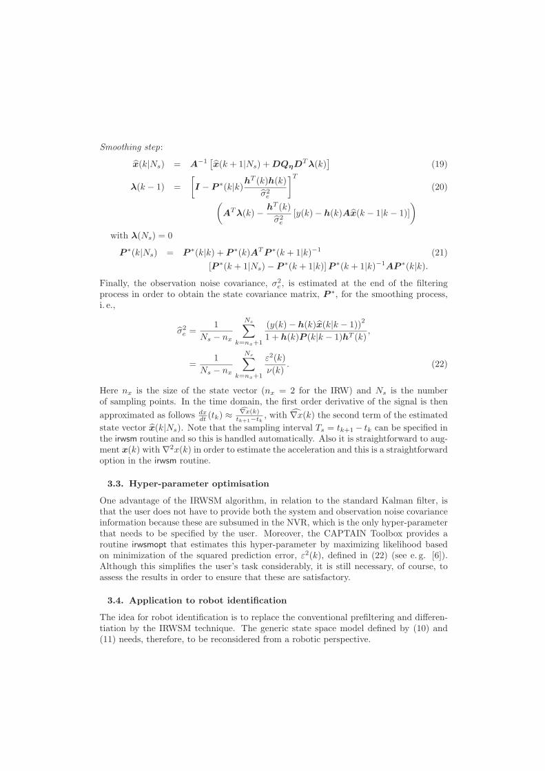
Smoothing step:

x(k|Ns) = A−1[x(k + 1|Ns) + DQηDT λ(k)

](19)

λ(k − 1) =

[I − P ∗(k|k)

hT (k)h(k)

σ2e

]T

(20)

(AT λ(k) −

hT (k)

σ2e

[y(k) − h(k)Ax(k − 1|k − 1)]

)

with λ(Ns) = 0

P ∗(k|Ns) = P ∗(k|k) + P ∗(k)AT P ∗(k + 1|k)−1 (21)

[P ∗(k + 1|Ns) − P ∗(k + 1|k)] P ∗(k + 1|k)−1AP ∗(k|k).

Finally, the observation noise covariance, σ2e , is estimated at the end of the filtering

process in order to obtain the state covariance matrix, P ∗, for the smoothing process,i. e.,

σ2e =

1

Ns − nx

Ns∑

k=nx+1

(y(k) − h(k)x(k|k − 1))2

1 + h(k)P (k|k − 1)hT (k),

=1

Ns − nx

Ns∑

k=nx+1

ε2(k)

ν(k). (22)

Here nx is the size of the state vector (nx = 2 for the IRW) and Ns is the numberof sampling points. In the time domain, the first order derivative of the signal is then

approximated as follows dxdt

(tk) ≈c∇x(k)

tk+1−tk, with ∇x(k) the second term of the estimated

state vector x(k|Ns). Note that the sampling interval Ts = tk+1 − tk can be specified inthe irwsm routine and so this is handled automatically. Also it is straightforward to aug-ment x(k) with ∇2x(k) in order to estimate the acceleration and this is a straightforwardoption in the irwsm routine.

3.3. Hyper-parameter optimisation

One advantage of the IRWSM algorithm, in relation to the standard Kalman filter, isthat the user does not have to provide both the system and observation noise covarianceinformation because these are subsumed in the NVR, which is the only hyper-parameterthat needs to be specified by the user. Moreover, the CAPTAIN Toolbox provides aroutine irwsmopt that estimates this hyper-parameter by maximizing likelihood basedon minimization of the squared prediction error, ε2(k), defined in (22) (see e. g. [6]).Although this simplifies the user’s task considerably, it is still necessary, of course, toassess the results in order to ensure that these are satisfactory.

3.4. Application to robot identification

The idea for robot identification is to replace the conventional prefiltering and differen-tiation by the IRWSM technique. The generic state space model defined by (10) and(11) needs, therefore, to be reconsidered from a robotic perspective.

Observation equation

Here, the output y(k) is replaced by the measured position of link j: qmj. By considering

the link j, we have the following relation for the measured position:

qmj(k) = qj(k) + qj(k), (23)

where qj(k) is the joint position measured at the kth sampling instant and qj(k) is thesensor noise. According to [1], this noise can be considered to be white with a covariance13∆2

q, where ∆q is the encoder resolution; and according to to [17], the Staubli R© TX40encoders’ resolution is 2 10−4 degrees per count. This is the robot considered later forthe experimental validation, which is a typical example of an industrial robot. If themeasurement noise is also assumed to be normally distributed, the observation relation(11) is valid and the noise standard deviation σe ≈ ∆q can be estimated from the robotperformance data sheet should it be required. Furthermore, the position qj(k) is equalto the state x(k) defined by (9).

State equation

There are two ways of retrieving the joint acceleration when using IRWSM:

• Applying the algorithm twice with Airwsm1 =

[1 10 1

];

• Applying the algorithm once with an augmented matrix Airwsm2 =

1 1 00 1 10 0 1

.

In the first case, the relevance of the random walk model is firstly investigated withAirwsm1. From equation (10),

IRWSM1 :

[qj(k)∇qj(k)

]=

[1 10 1

] [qj(k − 1)∇qj(k − 1)

]+

[1 00 1

] [0

η1,j(k − 1)

](24)

where the second state ∇qj represents the velocity, so that velocity information is notdriven by dynamic equations but by a random walk with a white noise input η1,j rep-resenting the unmodelled dynamics, effectively the modelling error. As explained in[24], this kind of model works for systems with slowly varying states. For robotic appli-cations, however, the controller requires high frequency sampling in order to have thelarge feedback gains required for more robust control; see e. g. [15]. For example, therobot considered in the next section 4 has a sampling rate of 5000 Hz. However, themechanical bandwidth is usually located below 10 Hz so, with the above IRW modelexpressed at the robot sampling frequency, the assumption of a slowly varying state issatisfied.

In the second case, using the augmented model trasition matrix Airwsm2, the velocityis driven by the acceleration, which is now defined as a random walk driven by a whitenoise input; and, as in the case of the velocity, the assumption of a slowly varying state

seems appropriate. From (10), the state equations in this case are as follows:

IRWSM2 :

qj(k)∇qj(k)∇2qj(k)

=

1 1 00 1 10 0 1

qj(k − 1)∇qj(k − 1)∇2qj(k − 1)

+

1 0 00 1 00 0 1

00

η2,j(k − 1)

.

(25)

Numerical approximation

The modelling error information can be retrieved from the tracking error, i. e.,

ǫtrj(k) = qrj

(k) − qmj(k) ∀ k = 1, 2, . . . , Ns, (26)

where qrj(k) is the reference trajectory of link j at the kth sampling instant. Of course ifthe model was perfect, the tracking error would be zero ∀ k. If the tracking error variation∆ǫtrj

(k) = ǫtrj(k)− ǫtrj

(k−1) is assumed to be a white and normally distributed noise,we have η1,j(k) ≈ ∆ǫtrj

(k). If the 2nd variation ∆2ǫtrjis then assumed to be white and

normally distributed noise, we have η2,j(k) ≈ ∆2ǫtrj(k). Finally, the NVR of link j can

be approximated by

NVRirwsm1

j =

(std(∆ǫtrj

)

∆qj

)2

(27)

NVRirwsm2

j =

(std(∆2ǫtrj

)

∆qj

)2

(28)

where ∆qjis the encoder resolution of link j and std(·) is the standard deviation. Ta-

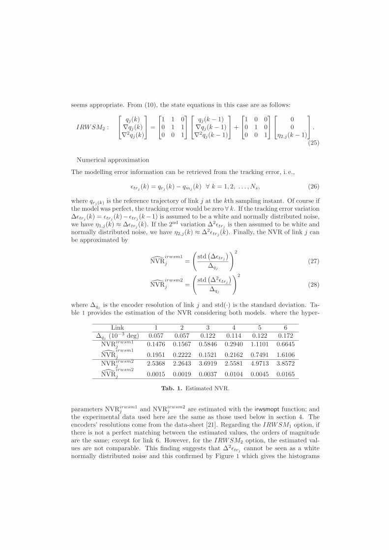
ble 1 provides the estimation of the NVR considering both models. where the hyper-

Link 1 2 3 4 5 6∆qj

(10−3 deg) 0.057 0.057 0.122 0.114 0.122 0.172

NVRirwsm1j 0.1476 0.1567 0.5846 0.2940 1.1101 0.6645

NVRirwsm1

j 0.1951 0.2222 0.1521 0.2162 0.7491 1.6106

NVRirwsm2j 2.5368 2.2643 3.6919 2.5581 4.9713 3.8572

NVRirwsm2

j 0.0015 0.0019 0.0037 0.0104 0.0045 0.0165

Tab. 1. Estimated NVR.

parameters NVRirwsm1j and NVRirwsm2

j are estimated with the irwsmopt function; andthe experimental data used here are the same as those used below in section 4. Theencoders’ resolutions come from the data-sheet [21]. Regarding the IRWSM1 option, ifthere is not a perfect matching between the estimated values, the orders of magnitudeare the same; except for link 6. However, for the IRWSM2 option, the estimated val-ues are not comparable. This finding suggests that ∆2ǫtrj

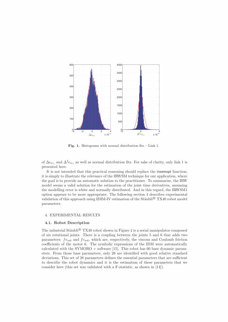
cannot be seen as a whitenormally distributed noise and this confirmed by Figure 1 which gives the histograms

−4 −2 0 2 4

x 10−5

0

100

200

300

400

500

600

∆ǫtr1

−5 0 5

x 10−6

0

500

1000

1500

2000

2500

3000

3500

4000

∆2ǫtr1

Fig. 1. Histograms with normal distribution fits – Link 1.

of ∆ǫtr1and ∆2ǫtr1

as well as normal distribution fits. For sake of clarity, only link 1 ispresented here.

It is not intended that this practical reasoning should replace the irwsmopt function;it is simply to illustrate the relevance of the IRWSM technique for our application, wherethe goal is to provide an automatic solution to the practitioner. To summarize, the IRWmodel seems a valid solution for the estimation of the joint time derivatives, assumingthe modelling error is white and normally distributed. And in this regard, the IRWSM1option appears to be more appropriate. The following section 4 describes experimentalvalidation of this approach using IDIM-IV estimation of the Staubli R© TX40 robot modelparameters.

4. EXPERIMENTAL RESULTS

4.1. Robot Description

The industrial Staubli R© TX40 robot shown in Figure 2 is a serial manipulator composedof six rotational joints. There is a coupling between the joints 5 and 6 that adds twoparameters: fvm6 and fcm6, which are, respectively, the viscous and Coulomb frictioncoefficients of the motor 6. The symbolic expressions of the IDM were automaticallycalculated with the SYMORO + software [15]. This robot has 60 base dynamic param-eters. From those base parameters, only 28 are identified with good relative standarddeviations. This set of 28 parameters defines the essential parameters that are sufficientto describe the robot dynamics and it is the estimation of these parameters that weconsider here (this set was validated with a F-statistic, as shown in [14]).

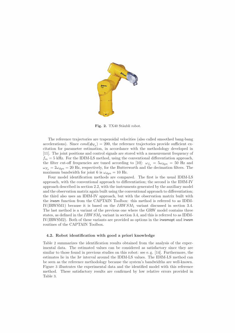
Fig. 2. TX40 Staubli robot.

The reference trajectories are trapezoidal velocities (also called smoothed bang-bangaccelerations). Since cond(φFp

) = 200, the reference trajectories provide sufficient ex-citation for parameter estimation, in accordance with the methodology developed in[11]. The joint positions and control signals are stored with a measurement frequency offm = 5 kHz. For the IDIM-LS method, using the conventional differentiation approach,the filter cut-off frequencies are tuned according to [10]: ωfq

= 5ωdyn = 50 Hz andωFp

= 2ωdyn = 20 Hz, respectively, for the Butterworth and the decimation filters. Themaximum bandwidth for joint 6 is ωdyn = 10 Hz.

Four model identification methods are compared. The first is the usual IDIM-LSapproach, with the conventional approach to differentiation; the second is the IDIM-IVapproach described in section 2.2, with the instruments generated by the auxiliary modeland the observation matrix again built using the conventional approach to differentiation;the third also uses an IDIM-IV approach, but with the observation matrix built withthe irwsm function from the CAPTAIN Toolbox: this method is referred to as IDIM-IV(IRWSM1) because it is based on the IRWSM1 variant discussed in section 3.4.The last method is a variant of the previous one where the GRW model contains threestates, as defined in the IRWSM2 variant in section 3.4, and this is referred to as IDIM-IV(IRWSM2). Both of these variants are provided as options in the irwsmopt and irwsm

routines of the CAPTAIN Toolbox.

4.2. Robot identification with good a priori knowledge

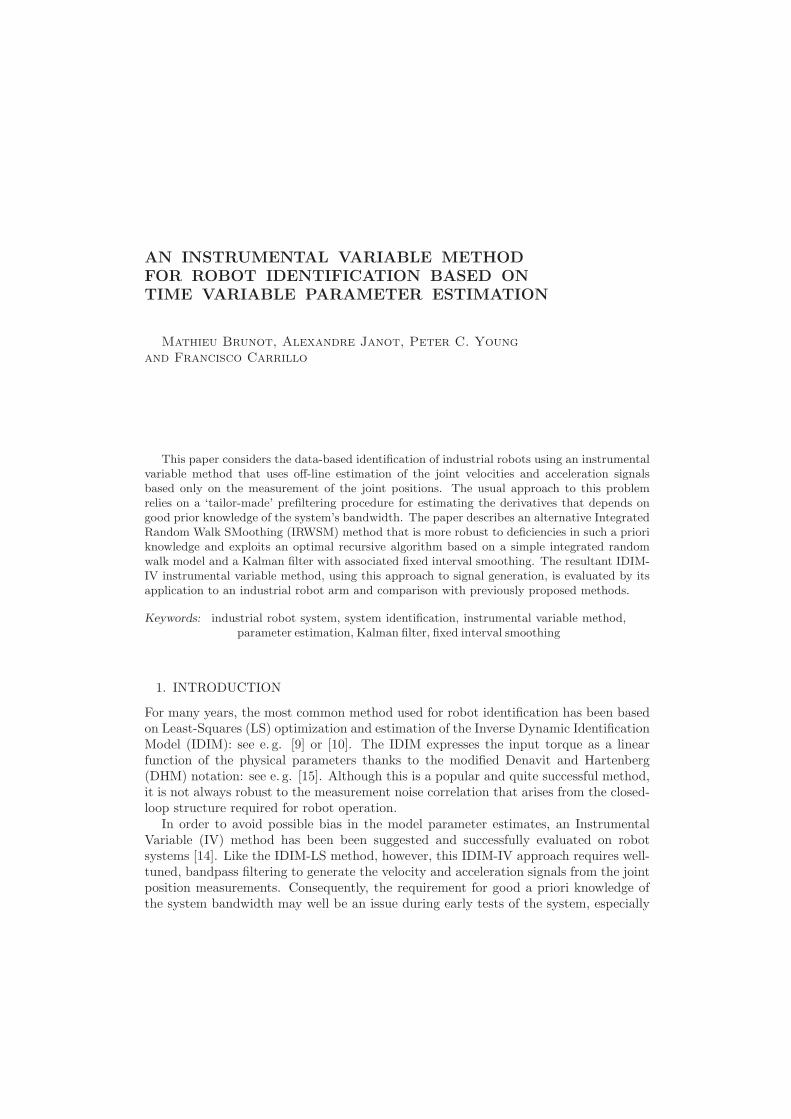
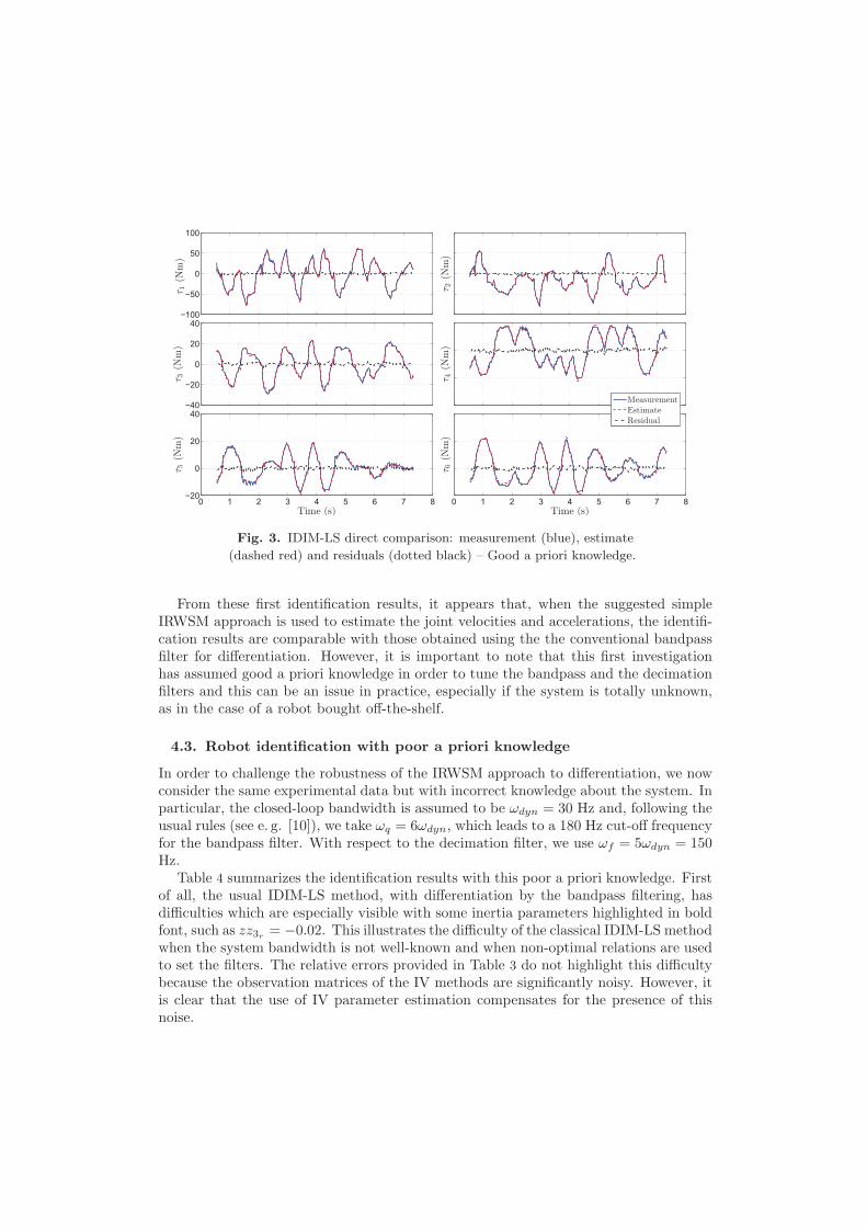
Table 2 summarizes the identification results obtained from the analysis of the exper-imental data. The estimated values can be considered as satisfactory since they aresimilar to those found in previous studies on this robot: see e. g. [14]. Furthermore, theestimates lie in the 3σ interval around the IDIM-LS values. The IDIM-LS method canbe seen as the reference methodology because the system’s bandwidths are well-known.Figure 3 illustrates the experimental data and the identified model with this referencemethod. These satisfactory results are confirmed by low relative errors provided inTable 3.

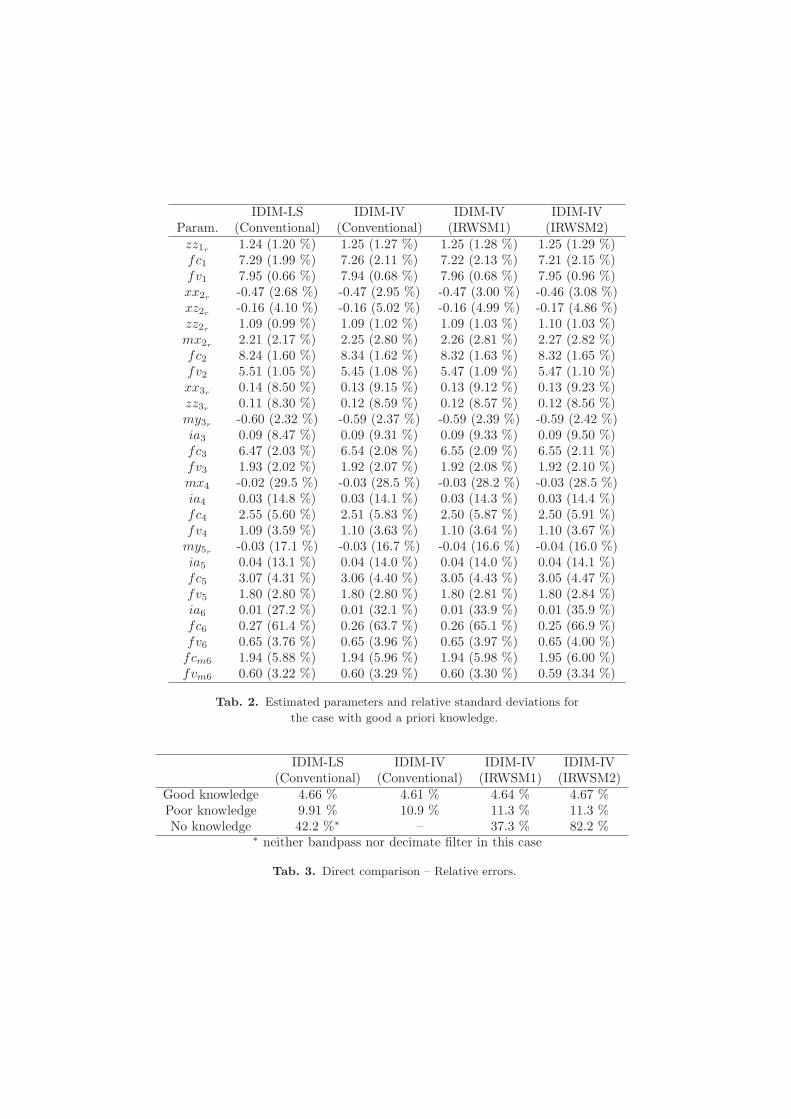
IDIM-LS IDIM-IV IDIM-IV IDIM-IVParam. (Conventional) (Conventional) (IRWSM1) (IRWSM2)zz1r

1.24 (1.20 %) 1.25 (1.27 %) 1.25 (1.28 %) 1.25 (1.29 %)fc1 7.29 (1.99 %) 7.26 (2.11 %) 7.22 (2.13 %) 7.21 (2.15 %)fv1 7.95 (0.66 %) 7.94 (0.68 %) 7.96 (0.68 %) 7.95 (0.96 %)xx2r

-0.47 (2.68 %) -0.47 (2.95 %) -0.47 (3.00 %) -0.46 (3.08 %)xz2r

-0.16 (4.10 %) -0.16 (5.02 %) -0.16 (4.99 %) -0.17 (4.86 %)zz2r

1.09 (0.99 %) 1.09 (1.02 %) 1.09 (1.03 %) 1.10 (1.03 %)mx2r

2.21 (2.17 %) 2.25 (2.80 %) 2.26 (2.81 %) 2.27 (2.82 %)fc2 8.24 (1.60 %) 8.34 (1.62 %) 8.32 (1.63 %) 8.32 (1.65 %)fv2 5.51 (1.05 %) 5.45 (1.08 %) 5.47 (1.09 %) 5.47 (1.10 %)xx3r

0.14 (8.50 %) 0.13 (9.15 %) 0.13 (9.12 %) 0.13 (9.23 %)zz3r

0.11 (8.30 %) 0.12 (8.59 %) 0.12 (8.57 %) 0.12 (8.56 %)my3r

-0.60 (2.32 %) -0.59 (2.37 %) -0.59 (2.39 %) -0.59 (2.42 %)ia3 0.09 (8.47 %) 0.09 (9.31 %) 0.09 (9.33 %) 0.09 (9.50 %)fc3 6.47 (2.03 %) 6.54 (2.08 %) 6.55 (2.09 %) 6.55 (2.11 %)fv3 1.93 (2.02 %) 1.92 (2.07 %) 1.92 (2.08 %) 1.92 (2.10 %)mx4 -0.02 (29.5 %) -0.03 (28.5 %) -0.03 (28.2 %) -0.03 (28.5 %)ia4 0.03 (14.8 %) 0.03 (14.1 %) 0.03 (14.3 %) 0.03 (14.4 %)fc4 2.55 (5.60 %) 2.51 (5.83 %) 2.50 (5.87 %) 2.50 (5.91 %)fv4 1.09 (3.59 %) 1.10 (3.63 %) 1.10 (3.64 %) 1.10 (3.67 %)

my5r-0.03 (17.1 %) -0.03 (16.7 %) -0.04 (16.6 %) -0.04 (16.0 %)

ia5 0.04 (13.1 %) 0.04 (14.0 %) 0.04 (14.0 %) 0.04 (14.1 %)fc5 3.07 (4.31 %) 3.06 (4.40 %) 3.05 (4.43 %) 3.05 (4.47 %)fv5 1.80 (2.80 %) 1.80 (2.80 %) 1.80 (2.81 %) 1.80 (2.84 %)ia6 0.01 (27.2 %) 0.01 (32.1 %) 0.01 (33.9 %) 0.01 (35.9 %)fc6 0.27 (61.4 %) 0.26 (63.7 %) 0.26 (65.1 %) 0.25 (66.9 %)fv6 0.65 (3.76 %) 0.65 (3.96 %) 0.65 (3.97 %) 0.65 (4.00 %)fcm6 1.94 (5.88 %) 1.94 (5.96 %) 1.94 (5.98 %) 1.95 (6.00 %)fvm6 0.60 (3.22 %) 0.60 (3.29 %) 0.60 (3.30 %) 0.59 (3.34 %)

Tab. 2. Estimated parameters and relative standard deviations for

the case with good a priori knowledge.

IDIM-LS IDIM-IV IDIM-IV IDIM-IV(Conventional) (Conventional) (IRWSM1) (IRWSM2)

Good knowledge 4.66 % 4.61 % 4.64 % 4.67 %Poor knowledge 9.91 % 10.9 % 11.3 % 11.3 %No knowledge 42.2 %∗ – 37.3 % 82.2 %

∗ neither bandpass nor decimate filter in this case

Tab. 3. Direct comparison – Relative errors.

−100

−50

0

50

100

τ 1(N

m)

τ 2(N

m)

−40

−20

0

20

40

τ 3(N

m)

τ 4(N

m)

0 1 2 3 4 5 6 7 8−20

0

20

40

τ 5(N

m)

Time (s)0 1 2 3 4 5 6 7 8

τ 6(N

m)

Time (s)

MeasurementEstimateResidual

Fig. 3. IDIM-LS direct comparison: measurement (blue), estimate

(dashed red) and residuals (dotted black) – Good a priori knowledge.

From these first identification results, it appears that, when the suggested simpleIRWSM approach is used to estimate the joint velocities and accelerations, the identifi-cation results are comparable with those obtained using the the conventional bandpassfilter for differentiation. However, it is important to note that this first investigationhas assumed good a priori knowledge in order to tune the bandpass and the decimationfilters and this can be an issue in practice, especially if the system is totally unknown,as in the case of a robot bought off-the-shelf.

4.3. Robot identification with poor a priori knowledge

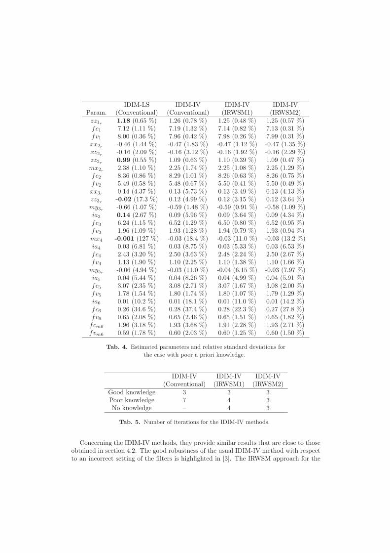
In order to challenge the robustness of the IRWSM approach to differentiation, we nowconsider the same experimental data but with incorrect knowledge about the system. Inparticular, the closed-loop bandwidth is assumed to be ωdyn = 30 Hz and, following theusual rules (see e. g. [10]), we take ωq = 6ωdyn, which leads to a 180 Hz cut-off frequencyfor the bandpass filter. With respect to the decimation filter, we use ωf = 5ωdyn = 150Hz.

Table 4 summarizes the identification results with this poor a priori knowledge. Firstof all, the usual IDIM-LS method, with differentiation by the bandpass filtering, hasdifficulties which are especially visible with some inertia parameters highlighted in boldfont, such as zz3r

= −0.02. This illustrates the difficulty of the classical IDIM-LS methodwhen the system bandwidth is not well-known and when non-optimal relations are usedto set the filters. The relative errors provided in Table 3 do not highlight this difficultybecause the observation matrices of the IV methods are significantly noisy. However, itis clear that the use of IV parameter estimation compensates for the presence of thisnoise.

IDIM-LS IDIM-IV IDIM-IV IDIM-IVParam. (Conventional) (Conventional) (IRWSM1) (IRWSM2)zz1r

1.18 (0.65 %) 1.26 (0.78 %) 1.25 (0.48 %) 1.25 (0.57 %)fc1 7.12 (1.11 %) 7.19 (1.32 %) 7.14 (0.82 %) 7.13 (0.31 %)fv1 8.00 (0.36 %) 7.96 (0.42 %) 7.98 (0.26 %) 7.99 (0.31 %)xx2r

-0.46 (1.44 %) -0.47 (1.83 %) -0.47 (1.12 %) -0.47 (1.35 %)xz2r

-0.16 (2.09 %) -0.16 (3.12 %) -0.16 (1.92 %) -0.16 (2.29 %)zz2r

0.99 (0.55 %) 1.09 (0.63 %) 1.10 (0.39 %) 1.09 (0.47 %)mx2r

2.38 (1.10 %) 2.25 (1.74 %) 2.25 (1.08 %) 2.25 (1.29 %)fc2 8.36 (0.86 %) 8.29 (1.01 %) 8.26 (0.63 %) 8.26 (0.75 %)fv2 5.49 (0.58 %) 5.48 (0.67 %) 5.50 (0.41 %) 5.50 (0.49 %)xx3r

0.14 (4.37 %) 0.13 (5.73 %) 0.13 (3.49 %) 0.13 (4.13 %)zz3r

-0.02 (17.3 %) 0.12 (4.99 %) 0.12 (3.15 %) 0.12 (3.64 %)my3r

-0.66 (1.07 %) -0.59 (1.48 %) -0.59 (0.91 %) -0.58 (1.09 %)ia3 0.14 (2.67 %) 0.09 (5.96 %) 0.09 (3.64 %) 0.09 (4.34 %)fc3 6.24 (1.15 %) 6.52 (1.29 %) 6.50 (0.80 %) 6.52 (0.95 %)fv3 1.96 (1.09 %) 1.93 (1.28 %) 1.94 (0.79 %) 1.93 (0.94 %)mx4 -0.001 (127 %) -0.03 (18.4 %) -0.03 (11.0 %) -0.03 (13.2 %)ia4 0.03 (6.81 %) 0.03 (8.75 %) 0.03 (5.33 %) 0.03 (6.53 %)fc4 2.43 (3.20 %) 2.50 (3.63 %) 2.48 (2.24 %) 2.50 (2.67 %)fv4 1.13 (1.90 %) 1.10 (2.25 %) 1.10 (1.38 %) 1.10 (1.66 %)

my5r-0.06 (4.94 %) -0.03 (11.0 %) -0.04 (6.15 %) -0.03 (7.97 %)

ia5 0.04 (5.44 %) 0.04 (8.26 %) 0.04 (4.99 %) 0.04 (5.91 %)fc5 3.07 (2.35 %) 3.08 (2.71 %) 3.07 (1.67 %) 3.08 (2.00 %)fv5 1.78 (1.54 %) 1.80 (1.74 %) 1.80 (1.07 %) 1.79 (1.29 %)ia6 0.01 (10.2 %) 0.01 (18.1 %) 0.01 (11.0 %) 0.01 (14.2 %)fc6 0.26 (34.6 %) 0.28 (37.4 %) 0.28 (22.3 %) 0.27 (27.8 %)fv6 0.65 (2.08 %) 0.65 (2.46 %) 0.65 (1.51 %) 0.65 (1.82 %)fcm6 1.96 (3.18 %) 1.93 (3.68 %) 1.91 (2.28 %) 1.93 (2.71 %)fvm6 0.59 (1.78 %) 0.60 (2.03 %) 0.60 (1.25 %) 0.60 (1.50 %)

Tab. 4. Estimated parameters and relative standard deviations for

the case with poor a priori knowledge.

IDIM-IV IDIM-IV IDIM-IV(Conventional) (IRWSM1) (IRWSM2)

Good knowledge 3 3 3Poor knowledge 7 4 3No knowledge – 4 3

Tab. 5. Number of iterations for the IDIM-IV methods.

Concerning the IDIM-IV methods, they provide similar results that are close to thoseobtained in section 4.2. The good robustness of the usual IDIM-IV method with respectto an incorrect setting of the filters is highlighted in [3]. The IRWSM approach for the

derivative estimation brings two advantages: firstly, the user does not have any concernsabout the settings of the bandpass filters; and secondly, as shown in Table 5, the IRWSMrequires less iterations to reach the convergence.

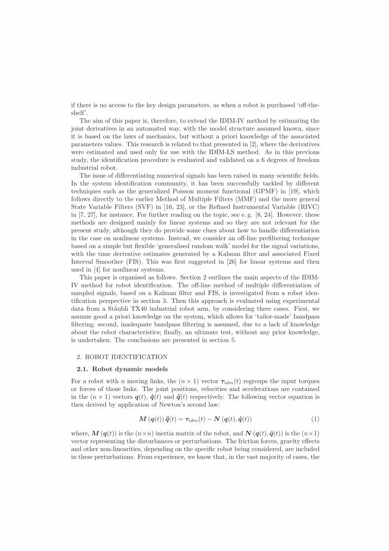
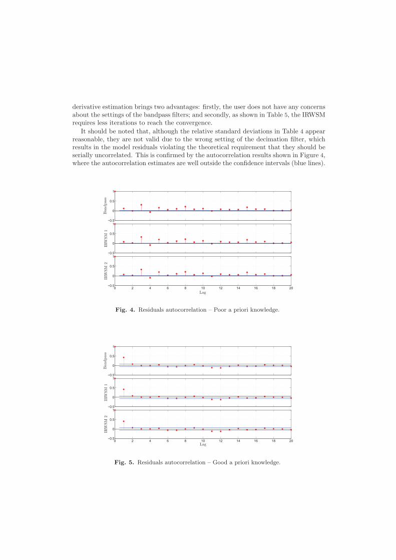
It should be noted that, although the relative standard deviations in Table 4 appearreasonable, they are not valid due to the wrong setting of the decimation filter, whichresults in the model residuals violating the theoretical requirement that they should beserially uncorrelated. This is confirmed by the autocorrelation results shown in Figure 4,where the autocorrelation estimates are well outside the confidence intervals (blue lines).

−0.5

0

0.5

1

Bandpass

−0.5

0

0.5

1

IRW

SM

1

0 2 4 6 8 10 12 14 16 18 20−0.5

0

0.5

1

Lag

IRW

SM

2

Fig. 4. Residuals autocorrelation – Poor a priori knowledge.

−0.5

0

0.5

1

Bandpass

−0.5

0

0.5

1

IRW

SM

1

0 2 4 6 8 10 12 14 16 18 20−0.5

0

0.5

1

Lag

IRW

SM

2

Fig. 5. Residuals autocorrelation – Good a priori knowledge.

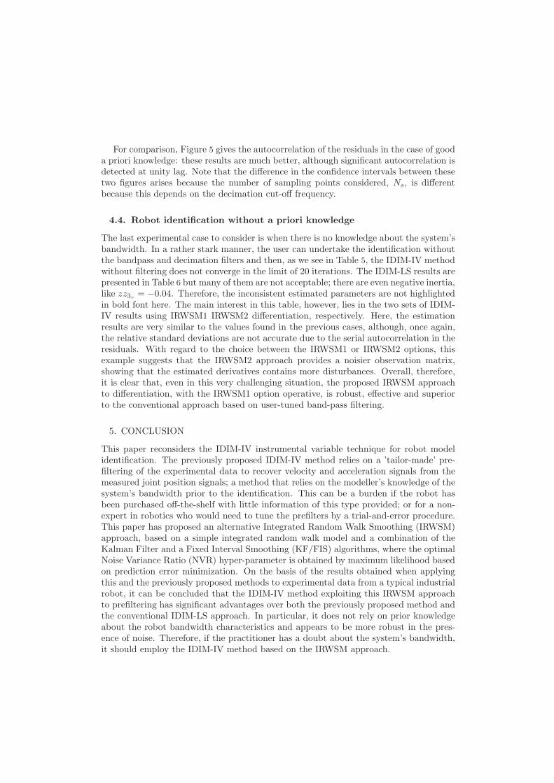
For comparison, Figure 5 gives the autocorrelation of the residuals in the case of gooda priori knowledge: these results are much better, although significant autocorrelation isdetected at unity lag. Note that the difference in the confidence intervals between thesetwo figures arises because the number of sampling points considered, Ns, is differentbecause this depends on the decimation cut-off frequency.

4.4. Robot identification without a priori knowledge

The last experimental case to consider is when there is no knowledge about the system’sbandwidth. In a rather stark manner, the user can undertake the identification withoutthe bandpass and decimation filters and then, as we see in Table 5, the IDIM-IV methodwithout filtering does not converge in the limit of 20 iterations. The IDIM-LS results arepresented in Table 6 but many of them are not acceptable; there are even negative inertia,like zz3r

= −0.04. Therefore, the inconsistent estimated parameters are not highlightedin bold font here. The main interest in this table, however, lies in the two sets of IDIM-IV results using IRWSM1 IRWSM2 differentiation, respectively. Here, the estimationresults are very similar to the values found in the previous cases, although, once again,the relative standard deviations are not accurate due to the serial autocorrelation in theresiduals. With regard to the choice between the IRWSM1 or IRWSM2 options, thisexample suggests that the IRWSM2 approach provides a noisier observation matrix,showing that the estimated derivatives contains more disturbances. Overall, therefore,it is clear that, even in this very challenging situation, the proposed IRWSM approachto differentiation, with the IRWSM1 option operative, is robust, effective and superiorto the conventional approach based on user-tuned band-pass filtering.

5. CONCLUSION

This paper reconsiders the IDIM-IV instrumental variable technique for robot modelidentification. The previously proposed IDIM-IV method relies on a ’tailor-made’ pre-filtering of the experimental data to recover velocity and acceleration signals from themeasured joint position signals; a method that relies on the modeller’s knowledge of thesystem’s bandwidth prior to the identification. This can be a burden if the robot hasbeen purchased off-the-shelf with little information of this type provided; or for a non-expert in robotics who would need to tune the prefilters by a trial-and-error procedure.This paper has proposed an alternative Integrated Random Walk Smoothing (IRWSM)approach, based on a simple integrated random walk model and a combination of theKalman Filter and a Fixed Interval Smoothing (KF/FIS) algorithms, where the optimalNoise Variance Ratio (NVR) hyper-parameter is obtained by maximum likelihood basedon prediction error minimization. On the basis of the results obtained when applyingthis and the previously proposed methods to experimental data from a typical industrialrobot, it can be concluded that the IDIM-IV method exploiting this IRWSM approachto prefiltering has significant advantages over both the previously proposed method andthe conventional IDIM-LS approach. In particular, it does not rely on prior knowledgeabout the robot bandwidth characteristics and appears to be more robust in the pres-ence of noise. Therefore, if the practitioner has a doubt about the system’s bandwidth,it should employ the IDIM-IV method based on the IRWSM approach.

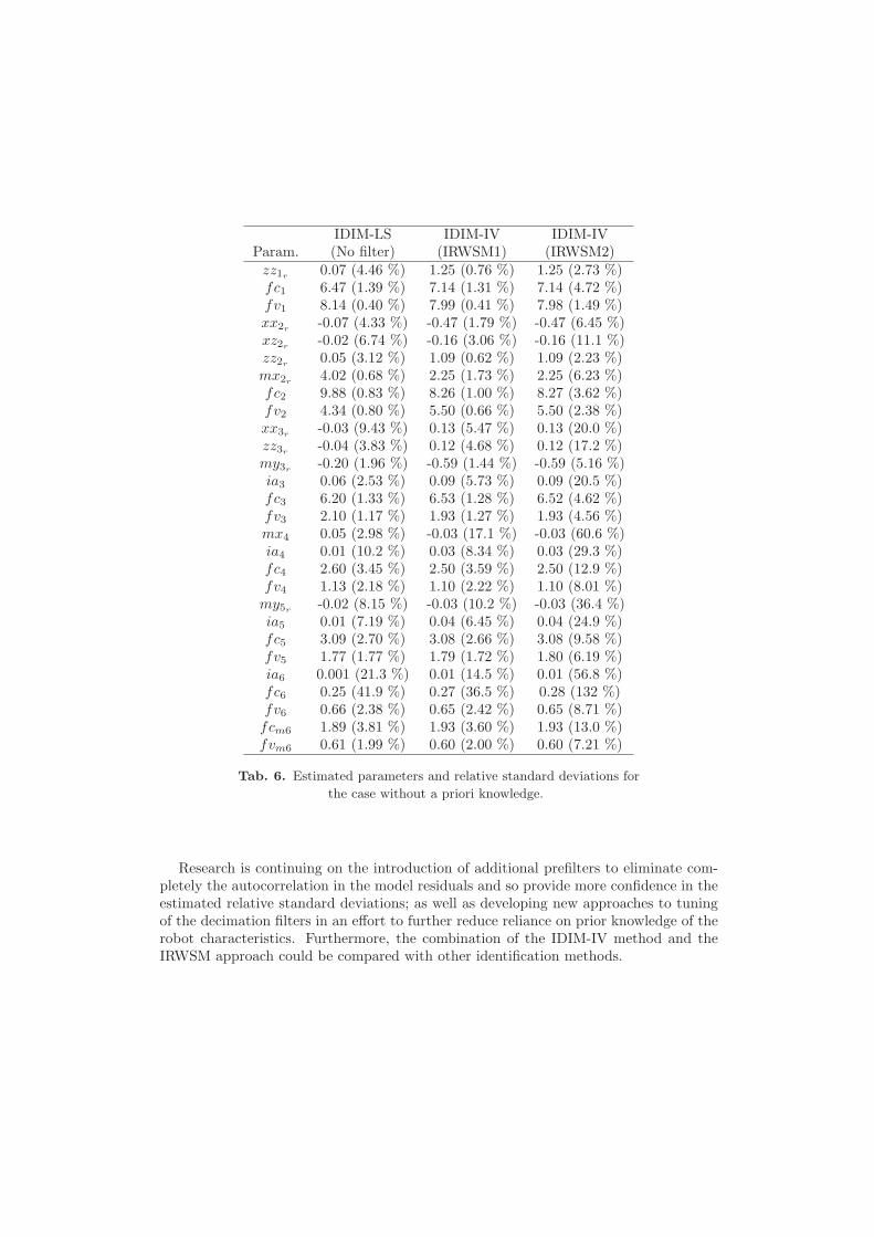
IDIM-LS IDIM-IV IDIM-IVParam. (No filter) (IRWSM1) (IRWSM2)zz1r

0.07 (4.46 %) 1.25 (0.76 %) 1.25 (2.73 %)fc1 6.47 (1.39 %) 7.14 (1.31 %) 7.14 (4.72 %)fv1 8.14 (0.40 %) 7.99 (0.41 %) 7.98 (1.49 %)xx2r

-0.07 (4.33 %) -0.47 (1.79 %) -0.47 (6.45 %)xz2r

-0.02 (6.74 %) -0.16 (3.06 %) -0.16 (11.1 %)zz2r

0.05 (3.12 %) 1.09 (0.62 %) 1.09 (2.23 %)mx2r

4.02 (0.68 %) 2.25 (1.73 %) 2.25 (6.23 %)fc2 9.88 (0.83 %) 8.26 (1.00 %) 8.27 (3.62 %)fv2 4.34 (0.80 %) 5.50 (0.66 %) 5.50 (2.38 %)xx3r

-0.03 (9.43 %) 0.13 (5.47 %) 0.13 (20.0 %)zz3r

-0.04 (3.83 %) 0.12 (4.68 %) 0.12 (17.2 %)my3r

-0.20 (1.96 %) -0.59 (1.44 %) -0.59 (5.16 %)ia3 0.06 (2.53 %) 0.09 (5.73 %) 0.09 (20.5 %)fc3 6.20 (1.33 %) 6.53 (1.28 %) 6.52 (4.62 %)fv3 2.10 (1.17 %) 1.93 (1.27 %) 1.93 (4.56 %)mx4 0.05 (2.98 %) -0.03 (17.1 %) -0.03 (60.6 %)ia4 0.01 (10.2 %) 0.03 (8.34 %) 0.03 (29.3 %)fc4 2.60 (3.45 %) 2.50 (3.59 %) 2.50 (12.9 %)fv4 1.13 (2.18 %) 1.10 (2.22 %) 1.10 (8.01 %)

my5r-0.02 (8.15 %) -0.03 (10.2 %) -0.03 (36.4 %)

ia5 0.01 (7.19 %) 0.04 (6.45 %) 0.04 (24.9 %)fc5 3.09 (2.70 %) 3.08 (2.66 %) 3.08 (9.58 %)fv5 1.77 (1.77 %) 1.79 (1.72 %) 1.80 (6.19 %)ia6 0.001 (21.3 %) 0.01 (14.5 %) 0.01 (56.8 %)fc6 0.25 (41.9 %) 0.27 (36.5 %) 0.28 (132 %)fv6 0.66 (2.38 %) 0.65 (2.42 %) 0.65 (8.71 %)fcm6 1.89 (3.81 %) 1.93 (3.60 %) 1.93 (13.0 %)fvm6 0.61 (1.99 %) 0.60 (2.00 %) 0.60 (7.21 %)

Tab. 6. Estimated parameters and relative standard deviations for

the case without a priori knowledge.

Research is continuing on the introduction of additional prefilters to eliminate com-pletely the autocorrelation in the model residuals and so provide more confidence in theestimated relative standard deviations; as well as developing new approaches to tuningof the decimation filters in an effort to further reduce reliance on prior knowledge of therobot characteristics. Furthermore, the combination of the IDIM-IV method and theIRWSM approach could be compared with other identification methods.

R E FE R E N C E S

[1] P .R. Belanger, P. Dobrovolny, A. Helmy, and X. Zhang: Estimation of angular velocityand acceleration from shaft-encoder measurements. Int. J. Robotics Research 17 (1998),1225–1233. DOI:10.1177/027836499801701107

[2] M. Brunot, A. Janot, and F. Carrillo: State Space Estimation Method for the Iden-tification of an Industrial Robot Arm. In: Proc. IFAC World Congress 50 (2017) 1,pp. 9815–9820.

[3] M. Brunot, A. Janot, F. Carrillo, H. Garnier, P.-O. Vandanjon, and M. Gautier: Physicalparameter identification of a one-degree-of-freedom electromechanical system operating inclosed loop. In: Proc. 17th IFAC Symposium on System Identification, 2015, pp. 823–828.DOI:10.1016/j.ifacol.2015.12.231

[4] D. Coca and S. A. Billings: A direct approach to identification of nonlinear differen-tial models from discrete data. Mech. Systems Signal Process. 13(5), (1999), 739–755.DOI:10.1006/mssp.1999.1230

[5] M. Dridi, G. Scorletti, M. Smaoui, and D. Tournier: From theoretical differentiationmethods to low-cost digital implementation. In: IEEE International Symposium on In-dustrial Electronics 2010, pp. 184–189. DOI:10.1109/isie.2010.5637595

[6] J. Durbin and S. J. Koopman: Time Series Analysis by State Space Methods. OxfordUniversity Press, 2012. DOI:10.1093/acprof:oso/9780199641178.001.0001

[7] H. Garnier, M. Gilson, P. C. Young, and E. Huselstein: An optimal IV technique foridentifying continuous-time transfer function model of multiple input systems. ControlEngrg. Practice 15 (2007), 471–486. DOI:10.1016/j.conengprac.2006.09.004

[8] H. Garnier, M. Mensler, and A. Richard: Continuous-time model identification fromsampled data: implementation issues and performance evaluation. Int. J. Control, 76(2003), 1337–1357. DOI:10.1080/0020717031000149636

[9] M. Gautier: Dynamic identification of robots with power model. In: Proc.IEEE International Conference on Robotics and Automation 3 (1997), 1922–1927.DOI:10.1109/robot.1997.619069

[10] M. Gautier, A. Janot, and P.-O. Vandanjon: A new closed-loop output error method forparameter identification of robot dynamics. IEEE Trans. Control Systems Technol. 21(2013), 428–444. DOI:10.1109/tcst.2012.2185697

[11] M. Gautier and W. Khalil: Exciting trajectories for the identification of baseinertial parameters of robots. Int. J. Robotics Research 11 (1992), 362–375.DOI:10.1177/027836499201100408

[12] M. Gilson, H. Garnier, P. C. Young, and P. M. J. Van den Hof: An instrumental variableapproach for rigid industrial robots identification. IET Control Theory Appl. 5 (2011),1147–1154. DOI:10.1049/iet-cta.2009.0476

[13] A. Janot, P.-O. Vandanjon, and M. Gautier: An instrumental variable approachfor rigid industrial robots identification. Control Engrg. Practice 25 (2014), 85–101.DOI:10.1016/j.conengprac.2013.12.009

[14] A. Janot, P.-O. Vandanjon, and M. Gautier: A generic instrumental variable approach forindustrial robot identification. IEEE Trans. Control Systems Technol. 22 (2014), 132–145.DOI:10.1109/tcst.2013.2246163

[15] W. Khalil and E. Dombre: Modeling, Identification and Control of Robots. Butterworth-Heinemann, 2004.

[16] K. Mahata and H. Garnier: Identification of continuous-time errors-in-variables models.Automatica 42 (2006), 1477–1490. DOI:10.1016/j.automatica.2006.04.012

[17] N. Marcassus, P.-O. Vandanjon, A. Janot, and M. Gautier: Minimal resolution neededfor an accurate parametric identification-application to an industrial robot arm. In: Proc.IEEE/RSJ International Conference on Intelligent Robots and Systems 2007, pp. 2455–2460. DOI:10.1109/iros.2007.4399476

[18] J. P. Norton: Optimal smoothing in the identification of linear time-varying sys-tems. In: Proc. of the Institution of Electrical Engineers 122 (1975), pp. 663–668.DOI:10.1049/piee.1975.0183

[19] G. P. Rao and H. Unbehauen: Identification of continuous-time systems. IEE Proc.Control Theory Appl. 153 (2006), 185–220. DOI:10.1049/ip-cta:20045250

[20] T. Soderstrom and P. Stoica: Instrumental Variable Methods for System Identification.Springer, 1983. DOI:10.1049/ip-cta:20045250

[21] Staubli Favergues: Arm – TX Series 40 Family. Staubli, 2015.

[22] J. M. Wooldridge: Introductory Econometrics: A Modern Approach. Fourth edition.South-Western, 2008.

[23] P. C. Young: An instrumental variable method for real-time identification of a noisyprocess Automatica, 6 (1970), 271–287. DOI:10.1016/0005-1098(70)90098-1

[24] P. C. Young: Recursive Estimation and Time-Series Analysis: An Introduction for TheStudent and Practitioner. Second edition. Springer Science and Business Media, 2012.

[25] P. C. Young: Refined instrumental variable estimation: Maximum likelihoodoptimization of a unified Box-Jenkins model. Automatica 52, (2015), 35–46.DOI:10.1016/j.automatica.2014.10.126

[26] P. C. Young, M. Foster, and M. Lees: A Direct Approach to the Identification andEstimation of Continuous-Time Systems From Discrete-Time Data Based on FixedInterval Smoothing. In: Proc. 12th IFAC World Congress 10 (1993), pp. 27–30.DOI:10.1016/s1474-6670(17)49207-x

[27] P. C. Young and A. J. Jakeman: Refined instrumental variable methods of time-seriesanalysis: Parts I, II and III Int. J. Control 29, 1-30; 30, 621–644, 31, (1979–1980),741–764. DOI:10.1080/00207178008961080

Mathieu Brunot, ONERA, 2 Avenue Edouard Belin, 31055 Toulouse, France; LGP ENI

Tarbes,47 avenue d’Azereix, BP 1629, 65016 Tarbes. France.

e-mail: Mathieu.Brunot@onera.fr

Alexandre Janot, ONERA, 2 Avenue Edouard Belin, 31055 Toulouse. France.

e-mail: Alexandre.Janot@onera.fr

Peter Young, Systems and Control Group, Lancaster Environment Centre, Lancaster

University, United Kingdom and Integrated Catchment Assessment and Management

Centre, Australian National University College of Medicine, Biology & Environment,

Canberra, ACT.

e-mail: p.young@lancaster.ac.uk

Francisco Carrillo, LGP ENI Tarbes, 47 avenue d’Azereix, BP 1629, 65016 Tarbes.

France.

e-mail: Francisco.Carrillo@enit.fr