Embed Size (px)
Citation preview

Corso di Laurea in Ingegneria InformaticaTesi di Laurea magistrale
An Integer Linear ProgrammingHeuristic for the Travelling
Salesman Problem
Candidato:Paolo Marchezzolo
Relatore:Chiar.mo Prof. Matteo Fischetti
11 Marzo 2013A.A. 2012/2013


A B S T R A C TThe Travelling Salesman Problem (TSP) is a well-known optimization
problem that has many applications in a wide array of fields. It is well-known that the TSP is a NP-hard problem, thus heuristic approaches arefundamental to be able to obtain good solutions in a reasonable amount oftime.
In this work, we explore a new heuristic approach to the TSP problem.We aim at improving an already existing solution by using a proximity ordistance function, and iteratively looking for improvements in the “neigh-borhood” of the provided solution. We iteratively solve two subproblems,called master and slave; the first is an ILP relaxation of the TSP without theSubtour Elimination Constraints that tries to find the cheaper solution (com-pared to the existing one) which is closer to the solution of the previousiteration, while the second tries to heuristically enforce the missing con-straints by finding the Shortest Spanning Tree that minimizes the HammingDistance with the main subproblem.
The thesis, in addition to a formal presentation of the aforementionedconcepts, also provides a computational analysis of the approach, testedover synthetically generated instances with various parameters settings.
The results of our testing show that our algorithm is consistently able tofind the optimal value in a reasonable amount of time over our test instances.While more specialized algorithms are much faster than the implementationprovided here, our approach still looks promising: it is more general, andcan easily be adapted to other NP-hard problems that currently do not havegood heuristics available; also, it is a new approach, so a higher degreeof optimization and improvement compared to already established ones ispredictable.
iii


C O N T E N T S1 the travelling salesman problem 1
1.1 Problem definition 1
1.2 Integer Linear Programming model 1
1.2.1 Linear Programming 1
1.2.2 Integer Linear Programming 2
1.2.3 An ILP model for the Travelling Salesman Problem 2
1.3 Relaxations of the ILP model 3
1.3.1 Relaxation by SECs elimination 3
1.3.2 1-tree relaxation 4
1.4 Some Heuristic approaches 5
1.4.1 Tour Construction Procedures 5
1.4.2 Tour Improvement Procedures 6
2 a new heuristic approach for the tsp 7
2.1 The basic idea 7
2.2 Distance function 7
2.3 The Master subproblem 8
2.4 The Slave subproblem 8
2.5 A first version of the algorithm 9
2.6 Step-by-step improvement 10
2.7 Stalling 12
2.8 A revised version of the algorithm 13
3 implementation 15
3.1 Data Structures 15
3.1.1 Graph representation 15
3.1.2 Solutions representation 16
3.1.3 Tabu list 16
3.1.4 Other data structures 16
3.2 The Master subproblem 16
3.2.1 CPLEX parameters setting 17
3.2.2 RINS Heuristic exploiting 18
3.3 The Slave subproblem 18
3.4 Main loop 19
3.5 Input and output 19
4 testing and experimental results 21
4.1 Test instances 21
4.2 Parameters to be tested 21
4.3 Test results 23
4.4 Test comments 27
5 conclusion 29
a software 31
a.1 Concorde 31
a.1.1 TSP Solver 31
a.1.2 Edge generation 31
a.1.3 TSPLIB format 32
v
vi contents
a.2 CPLEX 32
a.2.1 Interactive Solver 32
a.2.2 Callable Library 33
b source code 35
b.1 Main program 35
b.1.1 tandem.h 35
b.1.2 tandem.c 35
b.2 Kruskal implementation 50
b.2.1 kruskal.h 50
b.2.2 kruskal.c 51
b.3 Instance generation 52
b.3.1 script.sh 52
b.3.2 converter.c 52
b.3.3 merger.c 53
bibliography 55

L I S T O F F I G U R E SFigure 1 Example of swap of k edges for k = 2. 6
Figure 2 A sample execution of our algorithm 20
Figure 3 Evolution of master and slave values on Instance 11,with CPLEX_PARAM_INTSOLLIM=1 26
Figure 4 Evolution of master and slave values on Instance 11,with the RINS approach active 26
Figure 5 Evolution of master and slave values on Instance 9,with CPLEX_PARAM_INTSOLLIM=1 and binary search ac-tive 27
L I S T O F TA B L E STable 1 Test Instances 22
Table 2 Test Results, Instance 1 (300 nodes, 2243 edges) 22
Table 3 Test Results, Instance 2 (300 nodes, 4485 edges) 23
Table 4 Test Results, Instance 3 (300 nodes, 6728 edges) 23
Table 5 Test Results, Instance 4 (400 nodes, 3990 edges) 23
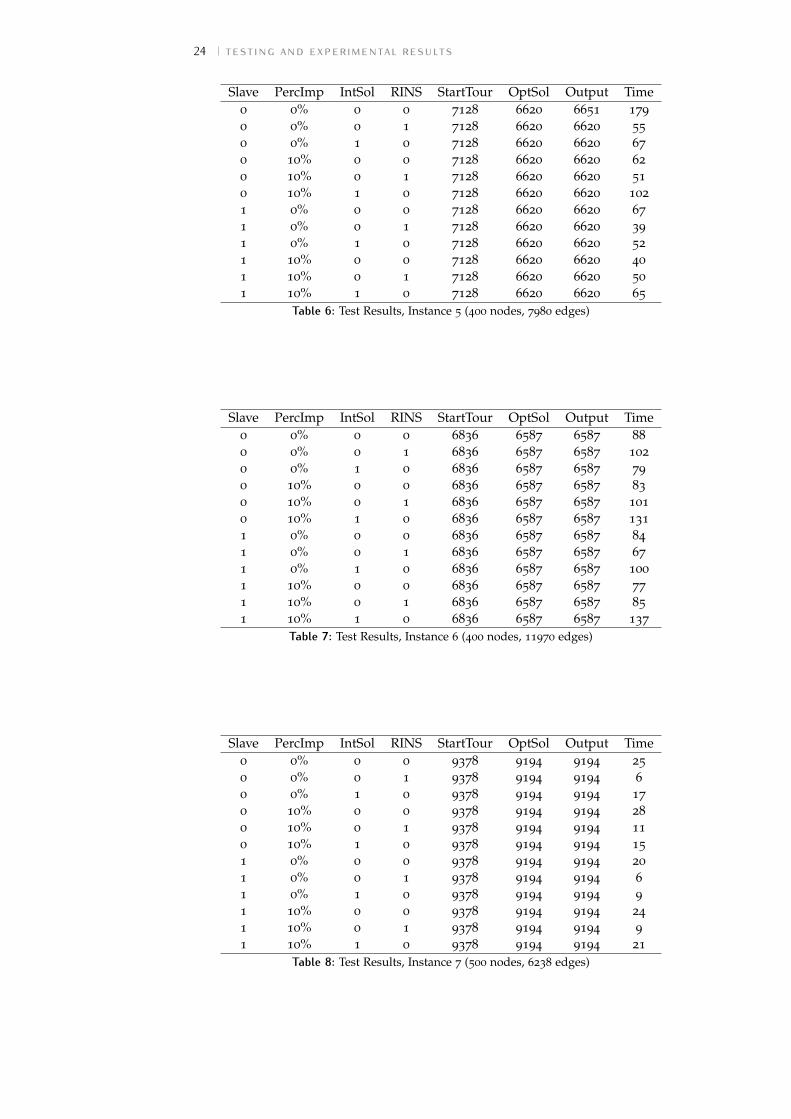
Table 6 Test Results, Instance 5 (400 nodes, 7980 edges) 24
Table 7 Test Results, Instance 6 (400 nodes, 11970 edges) 24
Table 8 Test Results, Instance 7 (500 nodes, 6238 edges) 24
Table 9 Test Results, Instance 8 (500 nodes, 12475 edges) 25
Table 10 Test Results, Instance 9 (500 nodes, 18713 edges) 25
Table 11 Test Results, Instance 10 (600 nodes, 8985 edges) 25
Table 12 Test Results, Instance 11 (600 nodes, 17970 edges) 26
vii


I N T R O D U C T I O N
overviewThe Travelling Salesman Problem (TSP) is one of the most relevant prob-
lems in combinatorial optimization, and has been widely studied in thefields of operational research and computer science. Informally it is the taskof finding the shortest route that, given a list of “cities” and their pairwisedistances, visits all of them once and returns to the origin “city”. It hasan extremely wide number of practical applications, ranging from planning,logistics and chip manifacturing to apparently unrelated ones, for exampleDNA sequencing.
Unfortunately, it is well-known that the TSP problem belongs to the classof NP-hard problems. This means that the time required to solve an ar-bitrary instance of the problem can, at worst, increase exponentially withthe size of said instance, making an exact algorithm unpractical for manyapplications.
For this reasons, heuristic algorithms are extremely important to obtain“acceptable” solutions in a reasonable amount of time. A very large amountof works investigates the task of finding an almost-optimal solution in shortcomputing time. Nowadays, we can find a good solution to instances withthousands, or even millions of “cities”, using modern heuristic methods.
Our work approaches the subject in a slightly different manner. As al-ready said, finding a good solution to even large instances is often nottoo difficult; however, it could be interesting to try to improve it further.To rephrase the concept, we will investigate if it is possible to find effec-tive algorithms that obtain a better solution by taking a “good” one as in-put. Obviously, we still aim at obtaining a heuristic method, since the NP-completeness of the problem still prevents us to reach an optimal solutionin a reasonable amount of time on some instances.
The main idea behind our algorithm is that, given a good solution to aTSP instance, it is likely that other good solutions (possibly better ones) arenot too far from the given one, using a suitable metric. Thus an effectivemethod that iteratively tries to lower the solution cost while minimizing thedistance from the incumbent could be effective in finding an improvement.This kind of heuristic would take advantage of the information containedin the given solution, providing a practical tool to use in combination withother heuristic methods.
ix

x List of Tables
content structurethe first chapter offers a brief introduction to the Travelling Salesman
Problem, its Integer Linear Programming formulation, relaxations ofthe model, and some exact and heuristic algorithms.
the second chapter introduces the particular approach to the TravellingSalesman Problem which is addressed in our work.
the third chapter presents in detail the implementation of the main top-ics of Chapter 2.
the fourth chapter reports the main experimental results found whiletesting the code.
the fifth chapter analyzes the outcome of the testing phase and out-lines possible future improvements of the ideas developed in our work.

1 T H E T R AV E L L I N G S A L E S M A NP R O B L E M
This chapter provides a brief introduction to the Travelling Salesman Prob-lem, along with definitions and concepts that will be used in following chap-ters. We formally define the TSP, give its ILP model and some relaxationsof it, and also illustrate some heuristic algorithms that can either create orimprove a tour for a given TSP instance.
1.1 problem definitionAn informal definition of the Travelling Salesman Problem was already
sketched in the introduction. A more precise one follows.
Definition 1. Given a weighted graph G = (V ,E) the Travelling SalesmanProblem requires to find a cycle such that:
1. every vertex v ∈ V is visited exactly once;
2. the weight (or cost) of the cycle is minimum.
If the graph is undirected, the problem is called Symmetric TravellingSalesman Problem (STSP). If the graph is directed, the problem is calledAsymmetric Travelling Salesman Problem (ATSP). The focus of this workis on the STSP variant of the problem. In the following, we will refer tothe undirected version when generically talking of the TSP problem unlessotherwise stated.
1.2 integer linear programming modelThe Travelling Salesman Problem is modeled in an elegant way as an
Integer Linear Programming problem. Since such approach will be widelyused in the rest of this work, a brief introduction to Linear Programmingand Integer Linear Programming is given.
1.2.1 Linear ProgrammingLinear Programming (LP) is a framework used to optimize a linear ob-
jective function subject to linear equality or inequality constraints. A LPproblem is usually stated as follows:
max cTx
Ax > b
x > 0
It is known that Linear Programming belongs to the P class, thus thereexists an algorithm that solves every instance of a LP problem in polynomial
1
2 the travelling salesman problem
time. Also, there exist practically efficient algorithms to solve these kindsof problems, like the simplex algorithm (which, despite not having a poly-nomial worst-case complexity, is often preferred thanks to many desirableproperties, for example the relative ease of adding new constraints to analready solved problem).
Unfortunately, the LP is not powerful enough to effectively model theTSP1. Representing a problem like the TSP requires some variables of the LPto be integer, which is possible in an Integer Linear Programming problem.
1.2.2 Integer Linear ProgrammingAn Integer Linear Programming problem looks exactly like a LP problem,
except that it allows to express integrality constraints over some variables ofthe model.
max cTx
Ax > b
x > 0 integer.
Adding integrality constraints to the model allows one to represent amuch broader class of problems than it was previously possible with LinearProgramming. In many cases, it is useful to force some variables to assumea value of either 0 or 1. Those variables are called binary variables, and areoften used when the model needs to make a “choice”; for example, as it willbe explained soon, in a TSP model, an edge is chosen in a solution only ifthe corresponding variable has a value of 1, and discarded otherwise.
However, an ILP model is, in its general case, NP-hard, which implies thelack of efficient, exact algorithms to solve a problems stated in that form.For this reason, heuristics for general ILP models are often the only way toapproach problems modeled as ILP for practical applications.
1.2.3 An ILP model for the Travelling Salesman ProblemAs already mentioned, the most natural way to represent mathematically
the TSP is using an ILP model. Using the notation intruduced in Definition1 and assuming that edge e ∈ E has a weight of we, we obtain the following:
min∑e∈E
wexe (1)
∑e∈δ(i)
xe = 2 i ∈ V (2)
∑e∈δ(S)
xe > 2 S ⊂ V , 2 6 |S| 6 |V |− 2 (3)
xe ∈ {0, 1} e ∈ E (4)
In the model, each variable xe is binary, as stated by the constraints (4),and each edge e is selected if and only if the corresponding variable xe is 1in the solution of the ILP. The set of constraints (2)2 ensures that each node
1 If it could, it would imply that the conjecture P = NP actually holds, while the opposite iswidely thought.
2 Notation δ(i) represents all the edges incident at i, and by extension δ(S) with S ∈ V is theset of all edges with one vertex in S and the other one outside S.
1.3 relaxations of the ilp model 3
has exactly two incident edges, and the constraints (3), called Subtour Elim-ination Constraints (SECs), are necessary to avoid subtours in the solution.
Constraints (3) can also be formulated in an alternative way: instead ofrequiring each subset of nodes S ∈ V to have at least two edges in their δ(S),it is also possible to force all the selected edges with both ends inside S tobe less or equal to |S|− 13:∑
e∈E(S)xe 6 |S|− 1 S ⊂ V , 3 6 |S| 6 |V |− 2 (5)
It is possible to show that the two forms (3) and (5) are equivalent toenforce the absence of subtours in the final solution. Both of them, however,include a number of constraints that increases exponentially with the sizeof the problem. So, not only solving the ILP model associated with a TSPproblem is a NP-hard problem itself, as described in Subsection 1.2.2, butthe size of the problem itself is also exponential. This makes impossible toutilize this model as-is for practical applications.
1.3 relaxations of the ilp modelSince, as already said in Subsection 1.2.3, trying to directly solve the ILP
formulation for the Travelling Salesman Problem is not a feasible approach,it is possible to relax some constraints of the formulation to obtain a solv-able model. Doing so may destroy the feasibility of the solution found, butallows us to obtain a lower bound of it in a reasonable amount of time.
Formally, a relaxation of a minimization problem (as the TSP is) is definedas follows:
Definition 2. Assume that our problem, P, is a minimization problem:
z = min f(x), x ∈ F(P).
Then a new problem R is defined as follows:
zR = min Φ(x), x ∈ F(R).
The problem R is called a relaxation of the problem P if the following condi-tions hold:
(a) F(P) ⊆ F(R)
(b) Φ(x) 6 f(x) ∀x ∈ F(P)
Two relaxations are mainly useful for this work, so a brief explanation ofthem is provided.
1.3.1 Relaxation by SECs eliminationThe first, and maybe most obvious idea to “simplify” the model is to just
remove the SECs. After doing so, the problem becomes both theoreticallyand practically easy.
This relaxation for the TSP model reads:
3 The set of all the edges with this property is written as E(S).

4 the travelling salesman problem
min∑e∈E
wexe (6)
∑e∈δ(i)
xe = 2 i ∈ V (7)
xe ∈ {0, 1} e ∈ E (8)
It is also possible to obtain an exact algorithm to solve the TSP from thisrelaxation by simply checking if each node is reachable from a fixed node.If the answer is positive, we have a solution of the original TSP; if not, theSECs corresponding to the subtours found in the current solution are addedto the model, that is solved again. Iterating this process, however, can atworst generate every SEC present in the original TSP formulation, severelydiminshing the approach’s usefulness.
1.3.2 1-tree relaxationAnother way to relax the TSP is to notice that, if the two edges incident
on some node (say, node 1) are removed from the solution, the remainingedges form a spanning tree on the subgraph induced by V \ {1}. Thus, anysolution of the TSP problem has the following structure:
(a) every node v 6= 1 has degree 2;
(b) the node 1 has two incident edges;
(c) removing the node 1 from the graph (and the two associated edges) weobtain a tree on the subgraph induced by V \ {1}.
Removing (a), we obtain a relaxed problem whose solution is:
1. find the Shortest Spanning Tree (SST) on the subgraph obtained re-moving the node 1;
2. add to the solution the cheapest two edges incident at node 1.
A solution constructed as previously described is called a 1-tree.An ILP model to solve the SST problem involved can be obtained easily
by the ILP model illustrated in Subsection 1.2.3.
min∑e∈E
wexe (9)
∑e∈δ(1)
xe = 2 (10)
∑e∈E
xe = n (11)
∑e∈δ(S)
xe > 1 S ⊂ V , 1 6 |S| 6 |V |− 2 (12)
xe ∈ {0, 1} e ∈ E (13)
The constraint (11) forces the solution to have exactly n selected edges, whileconstraint (10) ensures that two edges incident on node 1 are selected. Since

1.4 some heuristic approaches 5
the connection is guaranteed from the set of constraint (12), this ILP formu-lation is indeed a model of the 1-tree problem. However it is preferrableto not solve the 1-tree problem with an ILP solver, since the Shortest Span-ning Tree (SST) problem is solvable in polynomial time with simple greedyalgorithms, like Kruskal’s one4. The 1-tree relaxation can be easily obtainedafter having solved the SST over the graph induced by V \ {1} by just addingthe two cheapest edges incident on node 1.
1.4 some heuristic approachesThis section gives a brief outline of some simple heuristic approaches to
the Travelling Salesman Problem.
1.4.1 Tour Construction ProceduresThese heuristics work iteratively on the TSP instance they are processing.
To build the heuristic solution, they define three rules, that control the choiceof the starting node (or the starting subtour, depending on the method), theselection of the next node to be added to the solution, and the pair of nodeswhat will be the immediate predecessor and successor of the new node.Different choices for these rules generate different heuristics. We list threeexamples, that work better on average.
1. The Nearest Neighbour Algorithm starts from a random node on thegraph, then it selects the node that has the lowest distance from thelast picked node, and it adds it to the solution. The algorithm has atime complexity which is O(n2), where n is the number of nodes ofthe graph.
2. The Cheapest Insertion Algorithm chooses a random node at first, andits initial subtour is composed of the most “expensive” edge incidentfrom the first node. Then the algorithm iteratively chooses the nodethat minimizes the insertion cost of any unselected node between anypair of already selected nodes. The insertion cost of adding node k be-tween node i and node j is simply calculated as the difference betweenthe cost of the two edges (i,k) and (k, j) and the cost of the edge pre-viously part of the subtour (i, j). The algorithm has a time complexitywhich is O(n2 logn) for with graph of n nodes.
3. The Multi-Path Algorithm is somewhat similar to Kruskal’s algorithmto determine the Sortest Spanning Tree on a graph. It first sorts theedge set in nondecreasing order, then it starts examining the edges inthe sorted list. If an edge does not form a subtour with the alreadyselected ones and one of its vertices does have less than two incidentedges, then it is added to the solution. Considering a graph of nnodes, the algorithm terminates after selecting n edges, and its timecomplexity is 0(n2 logn).
These heuristic procedures will not be used in this work, however theycan be extremely valuable. They allow, in fact, to obtain a good solution ina very short amount of time; that solution can be then fed to our algorithm,which will try to improve it.
4 See Section 2.4 for additional details.

6 the travelling salesman problem
1.4.2 Tour Improvement ProceduresThese procedures start from an already existing solution and try to im-
prove it. The most natural idea to locally search for improvements whengiven a TSP solution is to swap out some edges and substitute them withsome others. More formally, if we consider a generic solution s describedwith its successor vector σ(i), i ∈ V , we can remove k edges from s andadd another k edges not previously in s. If k = 2, a possible example isshown in Figure 1; the edges (i,σ(i)) and (j,σ(j)) are removed and (i, j)and (σ(i),σ(j)) are added. The variation in the solution cost can be easilyevaluated:
∆C = −ci,σ(i) − cj,σ(j) + ci,j + cσ(i),σ(j)
The number of edges that have to be considered this way is O(nk).This strategy, apparently very simple, has been implemented with great
success by Lin & Kernighan, and is useful in many applications.
i j
σ(j) σ(i)
i j
σ(j) σ(2)
Figure 1: Example of swap of k edges for k = 2.
2 A N E W H E U R I S T I C A P P R OA C HF O R T H E T S P
This chapter presents the main ideas behind our approach: we define ourheuristic method and discuss its main implementative challenges.
2.1 the basic ideaIn this work, we aim at constructing a new algorithm that can improve an
existing solution of a TSP instance. While similar procedures already exist,like the one described in Subection 1.4.2, the problem will be tackled by adifferent perspective, as explained below.
The main idea behind our approach is that, given a good solution of theinstance, we can find a better solution by searching the “neighborhood” ofit. Hopefully, a good solution already contains a portion of the optimalsolution, and needs only a few changes in the set of selected edges to beimproved. We can then iteratively exploit such a procedure to lower thecost as much as possible, or until we reach a target cost, or we run out ofexecution time.
To do so, we need to define the distance between different solutions toa given TSP instance. After doing so, we will define a subproblem, calledmaster, using a particular ILP model that solves a relaxed version of the TSPformulation of Subsection 1.2.3 with some added constraints and a modi-fied objective function to take into account the distance between the twosolutions. Since the result is likely to violate one or more of the relaxatedconstraints, we will then use another procedure for the slave subproblem,which will try to enforce the constraints without going “too far” from thesolution of the master. Iteratively solving the master and the slave shouldproduce a succession of solutions which is likely to converge to a both im-proved and feasible solution, if not optimal.
The approach is somewhat inspired by previous works; in particular, [5]uses a similar approach while looking for feasible solutions instead of optimalones.
2.2 distance functionA solution of a TSP instance is easily represented as the set of values
the binary variables in its formulations assume. For this reason, the mostnatural way to define a distance function between two different solutions isto use a Hamming-like distance, which is basically equivalent to taking thebinary XOR of the two arrays and then summing over all the components.
More formally, given a TSP instance over the graph G = (V ,E), with|E| = n, and two solutions x = (x1, x2, . . . , xn) and x = (x1, x2, . . . , xn), thedistance between them will be defined as follows in the rest of this work:
∆(x, x) =n∑i=1
|xi − xi| (14)
7
8 a new heuristic approach for the tsp
2.3 the master subproblemAs already mentioned, we construct the Master subproblem as an ILP
problem that is based on a relaxation of the TSP general ILP model previ-ously presented. In particular, we will relax the subtour elimination con-straints, to obtain a model that can be actually handled by commercialsolvers. Then, instead of asking for the cheapest solution using the orig-inal edge costs, we want to retrieve the closest solution to the given one(which we will refer as x) that also costs less than a “target” parameter, T ,provided on input to the algorithm.
The ILP model follows.
min ∆(x, x) (15)∑e∈δ(i)
xe = 2 i ∈ V (16)
∑e∈E
wexe 6 T (17)
xe ∈ {0, 1} e ∈ E (18)
In other words, we avoid requiring the model to find us the largest costimprovement over the given solution. Instead we require to get the closestone which also happens to fulfill a provided cost requirement. This is donevia a modified objective function (15) which completely ignores the weightsw and just minimizes the distance function defined in Section 2.2. Theadditional constraint (17) ensures that any feasible solution of the modelsatisties our demand on the cost. The choice of T will be discussed in moredetail later.
The solution produced by this ILP is not feasible for the original TSP in-stance, in general. While being close to an another feasible solution is morelikely to fulfill all the SECs even if they are not included in the model, this isnot guaranteed, and the solution can contain subtours that prevent it to befeasible. For this reason, we need another procedure that heuristically triesto enforce those constraints without adding them to the ILP formulation.
2.4 the slave subproblemThe task that the slave subproblem performs is to try to remove any sub-
tour present in the output of the master. It does not need to necessarilyproduce a feasible solution for the TSP instance we are processing, it justneeds to select a set of edges that makes very unlikely to find subtours (orat least the same subtours that were already present) in the next iteration ofthe master subproblem.
While there are multiple ways to do so, a simple yet effective method toobtain this kind of effect in our specific application is to find a 1-tree overthe given graph, modifying each edge weight to properly mirror its presenceon the master output. The fact that a tree must be connected by definitionshould have the desired effect, forcing the outcome to break each subtour tobe connected with the remaining subgraph. Modifying the original weightsis also crucial since we do not want to completely destroy the informationscontained in the solution of the master.
2.5 a first version of the algorithm 9
That being said, the slave subproblem is defined as finding a 1-tree overthe graph underlying the TSP instance we are processing, where each edgee has the following weight:
we =M(1− x∗e) −Mx∗e +we (19)
=M(1− 2x∗e) +we
where x∗ is the 0-1 solution returned by the current master subproblem,and M is a constant such that:
M� we ∀e ∈ E.
This redefinition of the edges weights has the following meaning: alwaysprefer an edge already selected by the solution produced by the mastersubproblem; if two edges are both selected (or not selected) in the solutionof the master, then prefer the one that is cheaper in the original TSP instance.Defining the weights in this way makes “cheaper” for the slave to produce a1-tree which contains the greatest possible amount of edges already presentbeforehand, and thus is as close as possible to the master output whileensuring that all the nodes are reachable one from each other.
To actually solve the SST subproblem, we use a slightly modified ver-sion of the Kruskal’s algorithm. This choice is not immediately evidentwhile looking at the subproblem formulation, but becomes very clear to acloser analysis. The slave subproblem repeatedly solves a SST over the samegraph, and while the weights indeed depend on the x∗ vector produced bythe master, the possible values that we can assume are only two: M+weor −M+we. This is an obvious consequence of the fact that x∗ is a binaryvector. Since the Kruskal’s algorithm needs to sort the weights each time itruns, and then greedily sweeps the ordered array selecting the best edgesthat do not violate the tree structure, it would be very valuable to avoid re-peating this operation for each iteration of the algorithm. This is possible bysorting the edges by nonincreasing weight we‘ first, then at each iteration,create a copy of the sorted array and re-sort it, this time by nondecreasingvalue of x∗e; this operation can be implemented in linear time quite easily,as x∗e ∈ {0, 1}. This simple trick provides us a list which is sorted exactlyas it would be by utilitzing the we, but it does not need to compute them1,and it also avoids to perform multiple sortings. The computational cost ofperforming the Kruskal’s algorithm at each iterationg becomes then O(n),where n is the cardinality of the edge set E, and an initial overhead of com-plecity O(n logn) is performed only once at the start-up of our procedure.
2.5 a first version of the algorithmIn this section we will combine the master and slave subprocedures to
obtain a first version of the algorithm we aim at constructing. In addition tothe TSP instance and a solution of it that we want to improve, on input werequire a target T , which is the value we want to reach.
Here is a first pseudocode for our algorithm. The subproblems, masterand slave, are described in the previous two sections 2.3 and 2.4; we combinethem together as illustrated in Algorithm 1.
1 This also removes the problem of choosingM, that could be nontrivial if the application is notknown beforehand.

10 a new heuristic approach for the tsp
Data: A graph G = (V ,E),the weights we ∀e ∈ E,x solution of the TSP induced by G and w,a target value TResult: An improved solution xinitialize x to x;repeat
x∗ = solve the master with objective function ∆(x, x);x = solve the slave with weights defined as in (19);
until∑e∈Ewexe 6 T and x is a feasible solution of the TSP;
return xAlgorithm 1
So, in this first pseudocode, at each iteration we solve the master to find asolution better than the target T given in input, and then solve the slave, thatwill return a connected set of edges. We hope that the sequence of solutionsfound this way can eventually converge to a feasible solution of the initialTSP instance which is cheaper than T .
However, early analysis and testing of this approach allowed us to realizethat there are two issues that prevent the algorithm to perform efficiently(and even correctly) if using the implementation given.
1. Stalling: It is possible for the algorithm to loop indefinitely on a pair ofsolutions that solve respectively the master and the slave subproblem.In fact, there is not mechanism that prevents the master from returningmultiple times the same solution. This can be a problem, especially ifwe ask to reach a target T which is lower than the optimal TSP solutionfor that instance: the solution x∗ of the master will contain subtoursevery time (if the subproblem is feasible), and we have no way todetect such a situation.
2. If T is much lower than the cost of the provided solution x, it is un-reasonable to ask the master to return us a vastly improved solutionin one iteration; this basically destroys the meaning of our objectivefunction ∆(x, x): in fact, the master will be likely forced to choose asolution not that close to x to fulfill the cost constraint, thus losing thebenefits of searching locally for improvements.
3. It is unreasonable to ask a target T to be reached as a parameter for thealgorithm. The user will probably be interested in the best solutionwe can find within a prederetmined amount of time. It would bedesirable for the algorithm to not require such a parameter, and thenjust terminate if it can reach the optimal solution (and prove that isindeed optimal) or if it runs out of time.
In the following sections we discuss ideas to prevent stalling and to pre-serve locality. We will deal with points 2 and 3 first, since the solution tothe first one partially depends on the others.
2.6 step-by-step improvementAs already noticed in the previous section, it is not reasonable to ask
our ILP formulation to immediately find a solution not greater than T ,

2.6 step-by-step improvement 11
which is likely to be very low compared to the cost of our initial solutionx. Furthermore, requiring the user to provide T is itself not desirable, so weshould find a way to deal with this parameter internally.
To solve this issue, we implement a simple policy that handles the targetT internally. The idea is to lower the target by a tiny bit each time we findan improvement over the current best solution, and to let it unchanged ifwe do not find any in the current iteration. A first implementation of thisidea does the following:
1. Initialize T to (∑e∈Ewexe) − 1;
2. If the master or the slave finds a solution x that is feasible for theTSP instance we are considering, and is cheaper than the best solutionencountered until now, update T to (
∑e∈Ewexe) − 1.
This approach completely removes the need for the user to provide Texternally, and also allows the ILP model to improve more gradually, al-lowing to find solutions effectively close to the previous one. However, thedrawback is that the improvement proceeds slowly, since we only require aminimal improvement for each iteration.
To capture the best properties of both metods, we actually implementeda different update strategy for T , that slightly resembles the one we justpresented, but it tries to be a little more aggressive and lower the cost of thesolution more steadily if possible. This strategy is explained below:
1. Initialize a variable m to 110 that represents the minimum relative im-
provement that a solution needs to achieve in order to be consideredeffectively an “improvement”.
2. Initialize T to (1−m)∑e∈Ewexe;
3. If the master or the slave finds a solution x that is feasible for theTSP instance we are considering, and is cheaper than the best solutionencountered so far, update the incumbent x and redefine T to (1 −
m)∑e∈Ewexe;
4. If the master becomes infeasible at a certain iteration (i.e. we loweredtoo much T ), revert T to the last one that did not cause the master tobe unfeasible (call it Tp), then cut m in half and update T again as(1−m)
∑e∈Ewexe;
5. If m∑e∈Ewexe becomes smaller than one at any given iteration, fall
back to the previously proposed improvement strategy.
The rationale behind this approach is that we can ask for a fairly largeimprovement to our MIP model at first, since the initial tour is likely tobe far from the optimal solution, then we start lowering the minimum im-provement required as soon as we detect infeasible subproblems. When thefirst infeasible subproblem is detected, the update strategy for T turns intoa kind of binary search, that will lower m as much as it is needed to regainfeasibility of the master subproblem. This should,as hinted previously, al-low us to retain the advantages of both strategies, since we are progressingfaster than just lowering the solution by 1 every time.
However, we still are not guaranteed to obtain an unfeasible master sub-problem if T is lower than the optimal solution. While such a solutionis possible, the most likely scenario is a loop between an unfeasible and

12 a new heuristic approach for the tsp
cheaper-than-T master solution, and a feasible, but more expensive than Tslave solution. Without a stalling prevention mechanism, both strategiescannot detect when they have to stop, and the second one is likely to failcompletely.
2.7 stallingThe core issue with stalling is that nothing prevents the master to produce
the same solution twice. This situation is especially likely to show up if ourtarget value T is close to the optimal solution to our TSP instance. Whileobtaining an unfeasible master is possible, the more likely scenario is a loopas described in the previous section. A too low T will force subtours in themaster solution, and the slave subproblem is likely to be either more expen-sive than T or not a feasible TSP solution (if T is lower than the optimum,the slave solution cannot have both properties, obviously).
To avoid this problem, we implement an idea that is borrowed from thetechnique called tabu search. The tabu search is a local search method formathematical optimization problems, searching for improvements of a cur-rent solution in its neighborhood, but are likely to get stuck in local minima.To solve this problem, the tabu search keeps a tabu list, that is, a list of solu-tions that are “forbidden” for the algorithm to consider again within a shortamount of time.
In our case, the approach is slightly different. We will keep a tabu list ofsubtours, and each time the master subproblem is unfeasible, a subprocedurewill extract the shortest subtour and add it to the list. Then, the mastersubproblem is slightly redefined, with a little abuse of notation, as follows.
min ∆(x, x) (20)∑e∈δ(i)
xe = 2 i ∈ V (21)
∑e∈E
wexe 6 T (22)
∑e∈E(S)
xe 6 |S|− 1 S ∈ tabu list (23)
xe ∈ {0, 1} e ∈ E (24)
In this model we represented the tabu list as a set of subtour, which aresets of nodes that violate the constraints (5) explained in section 1.2.3.
The use of a tabu list approach has two positive effects on the algorithm,as previously mentioned:
• it removes the possibility of loops;
• it allows us to detect unfeasible subproblems.
The first point is straightforward. To better explain the second one, wenotice that the only thing that keeps the master subproblem from beinginfeasible is the fact that its solution can have subtours because of the re-laxation of the SECs. By adding the violated SECs to the formulation, wegradually disallow the only way the model has to provide a solution thatcosts less than T , and thus we force it to produce different values.

2.8 a revised version of the algorithm 13
This procedure can indeed generate all the SECs in the worst case, whichis obviously not tractable since solvers are unable to handle such a largeamount of constraints. We allow the user to provide the maximum size ofour tabu list, and if more subtours have to be added to it, older ones arereplaced with newer ones. The size of the model remains small this way,and the tabu list should fulfill its role in almost all cases (the exceptionbeing a particularly long loop of solutions with similar value, however this,while technically possible, is very unlikely and fixable by expanding themaximum tabu size).
2.8 a revised version of the algorithmAs a reference, we provide the pseudocode of our algorithm (Algorithm
2) after the modifications we illustrated in Sections 2.6 and 2.7.
The code is similar to the one already illustrated in Section 2.5. The keydifferences are already benn explained in the previous sections. In addi-tion, we now avoid solving the slave subproblem if the master subproblemupdated the value of T ; in that case, the master solution is already a validsolution of the underlying TSP instance, thus there is no need to try toheuristically enforce connectivity. The other slight difference, which is con-nected to the contents of Section 2.6 is that we check for improvements bothsolutions (slave and master), not only the output of the slave.
Data: A graph G = (V ,E),the weights we ∀e ∈ E,x solution of the TSP induced by G and wResult: An improved solution xinitialize x and ξ to x;initialize m and T as described in Section 2.6;while
∑e∈Ewexe > T or x is not a feasible solution for the TSP do
x∗ = solve the master with objective function ∆(x, ξ);if x∗ is feasible for the TSP and
∑e∈Ewex
∗e 6 T then
update T as described in Section 2.6;x = x∗;continue;
else if the master is unfeasible thenupdate T and m as described in Section 2.6;find the shortest subtour and add it to tabu list;
elsefind the shortest subtour and add it to tabu list;
endξ = slave optimal solution with weights defined as in (19);if ξ is feasible for the TSP and
∑e∈Eweξe 6 T then
x = ξ;update T as described in Section 2.6;
endendreturn x
Algorithm 2

14 a new heuristic approach for the tsp
This is the final version of our procedure, and its implementation will bediscussed in detail in the next chapter.

3 I M P L E M E N TAT I O N
In this chapter we will describe the main choices done and issues encoun-tered while implementing the ideas presented in Chapter 2.
The programming language chosen to code the algorithm is C, that ispreferred over any other high level programming language because of itsbetter efficiency and performance.
3.1 data structuresThe main data structures used in our implementation are quite simple.
The main things we need to represent are the graph underlying the TSP in-stance we process, and edge sets corresponding to various solutions to thesubproblems we solve. These data are stored in global variables, so eachfunction can access them freely and modify their value. This eases imple-mentation a bit, since we do not need to pass all the arrays multiple times tothe various function implemented. While this can hurt the reusability of thecode, most of it is quite specific to our particular application, and it is hardto imagine a practical situation in which this choice would create problems.
We illustrate briefly how such entities are implemented.
3.1.1 Graph representationTo represent our graph G = (V ,E), we implicitly number the nodes from
0 to |V |− 1. An edge e ∈ E has three attributes we want to keep track: thetwo vertices on which the edge is incident, and the cost of the edge. This isachieved with a simple struct shown below.
1 typedef struct edge{
2 double cost;
3 int first_node;
4 int second_node;
5 } edge;
This structure allows us to simply define the graph as an array of edges.In addition to this array, we create a data structure (called **nodes in thecode) that, for each node, mantains a list of each edge incident at that node.The list is implemented as an array of integers: for example, if nodes[0][a]has a certain value, then edges[nodes[0][a]] is an edge that is incident Tnode 0; the value of a is arbitrary. This data structure introduces a littleoverhead in terms of memory, however it saves time, especially for sparsegraphs, and allows us for an easier and more understandable implementa-tion.
15

16 implementation
3.1.2 Solutions representationEach solution of both the master or the slave subproblem is represented
as an array of binary integers of length |E|. The following edge sets are keptin memory throughout the execution of the algorithm:
• the solutions to the master subproblem at the present iteration and atthe previous one;
• the solutions to the slave subproblem at the present iteration and atthe previous one;
• the cheapest solution encountered that is feasible for the underlyingTSP instance.
3.1.3 Tabu listThe algorithm needs to keep and update a tabu list, whose details are
explained in Section 2.7. We coded this data structure in a slightly differentway than the one described previously. The table does not store the edge setsthat violate a SEC in the previous iterations, instead it directly memorizesthe corresponding SEC. This allow us to use a simple bidimensional arrayof integers to model the tabu list. The previously mentioned array (called**tabu) basically represents a matrix of coefficients; this eases the interactionwith the ILP solver utilized, since such a representation is close to the nativeone used by it. The list is empty at first, and is expanded whenever aviolated SEC is encountered.
3.1.4 Other data structuresThere is data structure that we did not illustrate in the previous section,
and is worth a brief mention. It is a sorted list of edges in order of nonde-creasing cost. This list is necessary for the considerations done in Section 2.4.It is implemented as an array of integers, called *sorted_list; if an integera is encountered before another integer b while sweeping the array from thefirst element to the last, this means that edges[a].cost is no greater thanedges[b].cost.
Other than that, every parameter that controls the execution of the algo-rithm (like the time limit iteration limit, the current target formerly referredas T , and other miscellaneous variables) are mostly kept global to allow anyprocedure to access it.
3.2 the master subproblemThe main implementative choice to do while implementing the master
subproblem defined in Section 2.3 is the one concerning the solver utilizedto obtain a solution of the master ILP model. We considered two mainalternatives to cover this functionality:
• Concorde1, a state-of-the-art TSP solver widely used in many applica-tions;
1 See Section A.1 for additional informations.
3.2 the master subproblem 17
• ILOG CPLEX, a commercial LP/ILP/MILP solver by IBM.
Utilizing Concorde is very desirable for our application: the ILP formula-tion is only slightly different from a common relaxation of the general ILPmodel, the only differences being the objective function and the additionalconstraint (17) Section 2.3. Concorde allows the insertion of custom con-straints; however, it handles them internally in hypergraph format, whichmakes very difficult to do so for our constraint.
For these reasons, we chose ILOG CPLEX as our solver. The CPLEX andCPLEX callable library functions we used are described in more detail inA.2.
We implemented a couple of subroutines to solve the master subproblem:
• solve_master() wraps the initialization of the ILP problem, the callsto CPLEX, and the updates to the target and to the tabu list;
• setproblemdata() initializes all the arrays that we need to pass toCPLEX for it to solve the ILP model;
• get_subtour() searches the current master solution for subtours, andreturns the shortest one if found;
• add_to_tabu_list() and new_sec() are used to keep the tabu list upto date; the SEC correspondent to the previously extracted subtour (ifany) is calculated and added to the tabu list.
3.2.1 CPLEX parameters settingSince the calls to the CPLEX solver in the master subproblem represent the
vast majority of the computational effort of our algorithm, we spent a fairamount of time trying to lower the time to complete the call, even at expenseof finding the optimal solution (as expected from a heuristic algorithm).
The first approach we adopted is the following. Since the whole algorithmis a heuristic method, it is not essential for CPLEX to return us the best so-lution that fulfills all the constraints; we can be fine with a reasonably goodone, too. Since CPLEX exploits heuristic methods before switching to anexact B&B strategy, we implemented the possibility to set to 1 the parameterCPLEX_PARAM_INTSOLLIM. Doing so forces CPLEX to stop after having foundone feasible solution, which will not be the closest one to the previous iter-ation, but will be “reasonably close” while saving a considerable amount ofcomputational time. This approach actually does not affect the optimality ofthe solution found, since we are just requiring a solution “reasonably close”to the previous one.
The second approach is aimed at avoiding an excessive computationaltime at each call to CPLEX. We limited the number of nodes of the decisiontree CPLEX uses internally to solve ILP problems to a fixed (and reasonablysmall) amount. If CPLEX exceeds this number, the problem is consideredunfeasible, so we either reduce the percentual improvement, if it happensduring a binary search, or terminate otherwise. This setting will be differ-entiated between binary search and the less aggressive approach, that havebeen presented in Section 2.6. We will describe the particular settings weused for these parameters in Chapter 4.
We also used a third approach, which deserves a separate section to bebetter explained.

18 implementation
3.2.2 RINS Heuristic exploitingThe CPLEX solver we used in the master subproblem employs a wide set
of heuristics. We are in particular interested to its RINS heuristic method.However, this method works best if CPLEX is provided with a starting fea-sible solution. Obviously we can not provide it, otherwise we would al-ready have a good solution to update our target and go further in the exe-cution. However, we can slightly modify the ILP model used in the masterto achieve this result:
min ∆(x, x) +Mz (25)∑e∈δ(i)
xe = 2 i ∈ V (26)
∑e∈E
wexe − z 6 T (27)
xe ∈ {0, 1} e ∈ E z > 0 integer. (28)
where M� 0 (50000 in our implementation).Using this variation allows us to always provide a feasible solution — the
best TSP solution found — since the model new can arbitrarily weaken thecutoff constraint.
Note that this approach is incompatible with CPLEX_PARAM_INTSOLLIM setto one (the algorithm would immediately stop, since the solution we pro-vide to it is already feasible). We instead used another parameter, CPLEX_PARAM_OBJDIF, which allows to do roughly the same: it tells CPLEX to stopwhen it encounters a solution costing less than M− 2n, where n = |V |; thismeans that the first solution with z = 0 is returned.
3.3 the slave subproblemThe slave subproblem is relatively unchallenging when it comes to imple-
mentation. As already explained in 2.4, a slightly modified version of theKruskal’s algorithm for the Shortest Spanning Tree is the core of the slavesubproblem. The only remaining task is to select the two cheapest edges in-cident on the excluded vertex (which is, in our case, the last one; the choiceof it is irrelevant anyway from a theoretical point of view, and doing soeases slightly the implementation), which is trivial.
The functions used for the slave subproblems are:
• solve_slave(), that is a wrapper for every other function call used forthe solution of the slave, in analogy with solve_master();
• kruskal_setup(), that is actually called in the main loop of our algo-rithm and not from the slave; however, it is described here since it isrelated to the custom implementation of Kruskal’s algorithm. Its func-tion is to fill the sorted list as described in Subsection 3.1.4, which isdone using a standard implementation of a Quicksort algorithm;
• kruskal(), that solves the SST problem defined in Section 2.4;
• has_subtour(), that is a wrapper for the previously defined get_sub
tour(); it returns zero if the graph is a feasible solution, and a nonzerovalue otherwise.

3.4 main loop 19
3.4 main loopThe only relevant aspect to mention about the main loop is the handling
of the stopping condition. We require the user to input both a time limitand an iteration limit; if either one is met at the end of any given iteration,the program stops. The only other fact that may cause the algorithm toterminate is bound to the update process described in Section 2.6: if we arelowering the target of one unit at a time, and we obtain an unfeasible master,we terminate. In fact, this means that the current best solution is optimalthanks to the assumption of having integer costs.
3.5 input and outputWe have two dedicated functions, parseinput() and print_results().
We briefly illustrate input and output formats, and the parameters that needto be passed to the algorithm for the parser to work correctly.
The function parseinput() implements a very basic parser for the inputfiles that represent the graph underlying the TSP instance we are processing,and the initial tour. In the edge file, the first row is required to contain thenumber of nodes and edges of the graph, then each subsequent line is atriple of integers that represents an edge: the first two integers are the twovertices on which the edge is incident, and the third one represents the cost.For a simple graph with 5 nodes and 7 edges, the file would look like this:
5 7
0 1 3
1 2 2
2 3 1
3 4 6
0 4 2
1 4 5
1 3 4
0
14
23
In the tour file, each line must contain only one integer, which representsa node. Reading the lines from the first one defines the edges of the startingtour. Obviously, each pair of nodes in the tour file must correspond to anedge on the edge file; if an illegal pair is detected, the parser halts andreturns an error message. This is a sample tour file for the previous graph:
0
1
2
3
4
0
14
23
The function print_results() prints on the file results.dat the best tourencountered in the execution of the algorithm. The format is the same usedfor the tour file.

20 implementation
Our routine also produces a log, that is extremely useful for monitoringthe algorithm’s performance. Various figures are reported, such as the Ham-ming distances between master and slave and the amount of nodes CPLEXused to solve the master, along with the values of the objective function (an“*” is displayed ach time an improvement is found). Below it is reported anexecution on a test instance.
Figure 2: A sample execution of our algorithm

4 T E S T I N G A N D E X P E R I M E N TA LR E S U LT S
In this chapter we describe the testing methodology we used to test thealgorithm, on which instances we did such testing, and the experimentalresults we gathered.
4.1 test instancesThe TSP instances we used to test the performance of our algorithm are
synthetic ones; they are produced using the following steps:
1. randomly choose a set of k points in R2 (also called point cloud), wherek is the number of desired nodes;
2. find a greedy tour in the instance defined by the nodes we just gener-ated and their distance on the plane;
3. randomly generate j edges starting from the point cloud;
4. merge the edges in the greedy tour with the randomly generated onesto obtain the initial edge list for our instance.
This procedure achieves two valuable objectives while generating an in-stace to be solved:
• it ensures that the graph has already a tour (the greedy one), so theTSP defined on that graph has surely a solution;
• it easily produces a good, but not optimal, tour that we can use toinitialize our algorithm.
The point cloud, the edge set, and the greedy tour are produced using theexecutable edgegen provided in the Concorde solver1. See also Appendix Bfor the code we used to generate our instances.
Table 1 illustrates the characteristics of our test instances.
4.2 parameters to be testedIn our tests, we ran our algorithm with a variety of settings, to verify
which set better works towards getting a good solution as soon as possible.We briefly describe them.
• Use of the slave subproblem: we are interested to see if the slave sub-problem effectively helps the algorithm to converge faster towards aheuristically good solution. We call this setting “Slave” in the follow-ing tables, and a value of 1 denotes an active slave, while a value of 0
means the opposite.
1 For more details, see Section A.1.
21

22 testing and experimental results
Number Nodes Edges Starting Tour Optimal Solution1 300 2243 4703 4661
2 300 4485 4490 4375
3 300 6728 4491 4311
4 400 3990 7104 6975
5 400 7980 7128 6620
6 400 11970 6836 6587
7 500 6238 9378 9194
8 500 12475 9301 9169
9 500 18713 9941 9117
10 600 8985 12791 12551
11 600 17970 13133 12437
Table 1: Test Instances
• Use of the binary search approach: we want to test if doing a binarysearch introduces an excessive amount of computational effort or if theexecution is sped up by this approach. This setting can be seen fromfield “PercImp” in our tables, that represent the minimum percentualimprovement at the starting iteration. We tested two possible values:0% (binary search disabled) and 10%. In the first case, we set thenumber of nodes CPLEX is allowed to explore in the decision tree to5000, while in the second case we use 50 nodes as long as the binarysearch is active, and 1000 nodes when it is disabled.
• Number of Integer Solutions limited to one: we want to check if thissetting effectively speeds up the exectution, as we hope. The param-eter is noted as “IntSol” in our tables, and has been set to one if thetables reports an 1, and let to its defult value (+∞) otherwise.
• Use of the z – RINS approach: it is very interesting to see if and howmuch RINS speeds up the computation. Again, this is marked as“RINS” in our tables, and a value of 0 means the normal approach,while a value of 1 refers to the one explained in 3.2.2.
Slave PercImp IntSol RINS StartTour OptSol Output Time0 0% 0 0 4703 4661 4661 1
0 0% 0 1 4703 4661 4661 2
0 0% 1 0 4703 4661 4661 1
0 10% 0 0 4703 4661 4661 2
0 10% 0 1 4703 4661 4661 2
0 10% 1 0 4703 4661 4661 2
1 0% 0 0 4703 4661 4661 1
1 0% 0 1 4703 4661 4661 1
1 0% 1 0 4703 4661 4661 1
1 10% 0 0 4703 4661 4661 2
1 10% 0 1 4703 4661 4661 1
1 10% 1 0 4703 4661 4661 3
Table 2: Test Results, Instance 1 (300 nodes, 2243 edges)

4.3 test results 23
4.3 test resultsWe include a number of tables that illustrate the test results we obtained.
Note that the fields “StartTour”, “OptSol”, “Output” actually refer to theobjective function value, not to the solution itself.
Slave PercImp IntSol RINS StartTour OptSol Output Time0 0% 0 0 4490 4375 4375 28
0 0% 0 1 4490 4375 4375 18
0 0% 1 0 4490 4375 4375 29
0 10% 0 0 4490 4375 4375 32
0 10% 0 1 4490 4375 4375 26
0 10% 1 0 4490 4375 4375 41
1 0% 0 0 4490 4375 4375 20
1 0% 0 1 4490 4375 4375 16
1 0% 1 0 4490 4375 4375 24
1 10% 0 0 4490 4375 4375 29
1 10% 0 1 4490 4375 4375 33
1 10% 1 0 4490 4375 4375 44
Table 3: Test Results, Instance 2 (300 nodes, 4485 edges)
Slave PercImp IntSol RINS StartTour OptSol Output Time0 0% 0 0 4491 4311 4311 60
0 0% 0 1 4491 4311 4311 71
0 0% 1 0 4491 4311 4311 53
0 10% 0 0 4491 4311 4324 31
0 10% 0 1 4491 4311 4311 43
0 10% 1 0 4491 4311 4311 84
1 0% 0 0 4491 4311 4311 59
1 0% 0 1 4491 4311 4311 70
1 0% 1 0 4491 4311 4311 48
1 10% 0 0 4491 4311 4312 45
1 10% 0 1 4491 4311 4311 38
1 10% 1 0 4491 4311 4313 73
Table 4: Test Results, Instance 3 (300 nodes, 6728 edges)
Slave PercImp IntSol RINS StartTour OptSol Output Time0 0% 0 0 7104 6975 6975 19
0 0% 0 1 7104 6975 6975 7
0 0% 1 0 7104 6975 6975 13
0 10% 0 0 7104 6975 6975 34
0 10% 0 1 7104 6975 6975 21
0 10% 1 0 7104 6975 6975 26
1 0% 0 0 7104 6975 6975 38
1 0% 0 1 7104 6975 6975 12
1 0% 1 0 7104 6975 6975 10
1 10% 0 0 7104 6975 6975 21
1 10% 0 1 7104 6975 6975 25
1 10% 1 0 7104 6975 6975 29
Table 5: Test Results, Instance 4 (400 nodes, 3990 edges)
24 testing and experimental results
Slave PercImp IntSol RINS StartTour OptSol Output Time0 0% 0 0 7128 6620 6651 179
0 0% 0 1 7128 6620 6620 55
0 0% 1 0 7128 6620 6620 67
0 10% 0 0 7128 6620 6620 62
0 10% 0 1 7128 6620 6620 51
0 10% 1 0 7128 6620 6620 102
1 0% 0 0 7128 6620 6620 67
1 0% 0 1 7128 6620 6620 39
1 0% 1 0 7128 6620 6620 52
1 10% 0 0 7128 6620 6620 40
1 10% 0 1 7128 6620 6620 50
1 10% 1 0 7128 6620 6620 65
Table 6: Test Results, Instance 5 (400 nodes, 7980 edges)
Slave PercImp IntSol RINS StartTour OptSol Output Time0 0% 0 0 6836 6587 6587 88
0 0% 0 1 6836 6587 6587 102
0 0% 1 0 6836 6587 6587 79
0 10% 0 0 6836 6587 6587 83
0 10% 0 1 6836 6587 6587 101
0 10% 1 0 6836 6587 6587 131
1 0% 0 0 6836 6587 6587 84
1 0% 0 1 6836 6587 6587 67
1 0% 1 0 6836 6587 6587 100
1 10% 0 0 6836 6587 6587 77
1 10% 0 1 6836 6587 6587 85
1 10% 1 0 6836 6587 6587 137
Table 7: Test Results, Instance 6 (400 nodes, 11970 edges)
Slave PercImp IntSol RINS StartTour OptSol Output Time0 0% 0 0 9378 9194 9194 25
0 0% 0 1 9378 9194 9194 6
0 0% 1 0 9378 9194 9194 17
0 10% 0 0 9378 9194 9194 28
0 10% 0 1 9378 9194 9194 11
0 10% 1 0 9378 9194 9194 15
1 0% 0 0 9378 9194 9194 20
1 0% 0 1 9378 9194 9194 6
1 0% 1 0 9378 9194 9194 9
1 10% 0 0 9378 9194 9194 24
1 10% 0 1 9378 9194 9194 9
1 10% 1 0 9378 9194 9194 21
Table 8: Test Results, Instance 7 (500 nodes, 6238 edges)

4.3 test results 25
Slave PercImp IntSol RINS StartTour OptSol Output Time0 0% 0 0 9301 9169 9169 86
0 0% 0 1 9301 9169 9169 91
0 0% 1 0 9301 9169 9169 114
0 10% 0 0 9301 9169 9169 74
0 10% 0 1 9301 9169 9169 72
0 10% 1 0 9301 9169 9169 120
1 0% 0 0 9301 9169 9169 84
1 0% 0 1 9301 9169 9169 63
1 0% 1 0 9301 9169 9169 132
1 10% 0 0 9301 9169 9169 92
1 10% 0 1 9301 9169 9169 69
1 10% 1 0 9301 9169 9169 120
Table 9: Test Results, Instance 8 (500 nodes, 12475 edges)
Slave PercImp IntSol RINS StartTour OptSol Output Time0 0% 0 0 9941 9117 9235 282
0 0% 0 1 9941 9117 9117 345
0 0% 1 0 9941 9117 9117 363
0 10% 0 0 9941 9117 9117 204
0 10% 0 1 9941 9117 9117 168
0 10% 1 0 9941 9117 9118 319
1 0% 0 0 9941 9117 9117 244
1 0% 0 1 9941 9117 9117 149
1 0% 1 0 9941 9117 9117 228
1 10% 0 0 9941 9117 9122 168
1 10% 0 1 9941 9117 9117 171
1 10% 1 0 9941 9117 9117 381
Table 10: Test Results, Instance 9 (500 nodes, 18713 edges)
Slave PercImp IntSol RINS StartTour OptSol Output Time0 0% 0 0 12791 12551 12643 42
0 0% 0 1 12791 12551 12551 25
0 0% 1 0 12791 12551 12551 39
0 10% 0 0 12791 12551 12551 63
0 10% 0 1 12791 12551 12551 45
0 10% 1 0 12791 12551 12551 91
1 0% 0 0 12791 12551 12551 56
1 0% 0 1 12791 12551 12551 36
1 0% 1 0 12791 12551 12551 46
1 10% 0 0 12791 12551 12551 66
1 10% 0 1 12791 12551 12551 38
1 10% 1 0 12791 12551 12551 84
Table 11: Test Results, Instance 10 (600 nodes, 8985 edges)

26 testing and experimental results
Slave PercImp IntSol RINS StartTour OptSol Output Time0 0% 0 0 13133 12437 12437 125
0 0% 0 1 13133 12437 12437 64
0 0% 1 0 13133 12437 12437 86
0 10% 0 0 13133 12437 12437 149
0 10% 0 1 13133 12437 12437 60
0 10% 1 0 13133 12437 12437 98
1 0% 0 0 13133 12437 12437 137
1 0% 0 1 13133 12437 12437 69
1 0% 1 0 13133 12437 12437 89
1 10% 0 0 13133 12437 12437 121
1 10% 0 1 13133 12437 12439 60
1 10% 1 0 13133 12437 12439 85
Table 12: Test Results, Instance 11 (600 nodes, 17970 edges)
Figure 3: Evolution of master and slave values on Instance 11, withCPLEX_PARAM_INTSOLLIM=1
Figure 4: Evolution of master and slave values on Instance 11, with the RINS ap-proach active

4.4 test comments 27
Figure 5: Evolution of master and slave values on Instance 9, withCPLEX_PARAM_INTSOLLIM=1 and binary search active
4.4 test commentsThere are a couple of observations we can draw from the results of these
tests.The first one is that our algorithm, even with the limitation to the number
of nodes, manages to find the optimal solution with almost all parametersettings, and with almost every instance. This is a positive thing, in a sense,however it may suggest a “not sufficiently heuristic” approach to the prob-lem. It would be interesting to repeat the tests with different settings for thenode limits, however this was not possible because of strict time constraintsfor the completion of our work.
The second one is that it does not emerge a clear winner between all theapproaches tested. This is partly expected, since many of the settings canwork well for a particular instance and not-so-well for another one. A moreextensive testing would help in better outlining which approach, on average,yields the best results, and which one should be avoided. The impressionis that both exploiting RINS heuristic and the limit of the number of integersolutions to one can greatly help the algorithm to reduce it execution time,although in some runs this effect is much less prominent. Furthermore,the binary search is probably the less successful expedient to speed up thecomputation: it is required a large amount of effort to effectively show thatthe current percentual improvement is too high, and while each updateimproves a lot the best solution, it is not worth it when compared to small,but very frequent updates by the less aggressive approach.
The plots provided also show how the master subproblem seems to “lead”the computation; the slave often produce edge sets with a very high cost justto enforce connection. This phenomenon is more pronounced if the binarysearch is active, as one can see in Figure 5, and may suggest a secondaryrole of the slave in the computation.


5 C O N C L U S I O NIn this work, we outlined and described a new approach for a heuristic
Tour Improvement Procedure for the TSP problem, based on the concept ofproximity. A variety of different parameter settings and slightly differentimplementations is proposed and evaluated with extensive testing.
The results of our testing suggest that many of the proposed parame-ter settings help to reduce the execution time of the algorithm, althoughnone of them has a dramatic impact on it. A more in-depth tuning phasecould help to further improve the performance of the algorithm, and to bet-ter grasp the interactions between our ILP formulation and the heuristicsCPLEX employs internally. Since the approach is new, we are confident thatthe performances of our algorithm can be improved significantly.
The final outcome of our research looks indeed promising, although notvery interesting as-is. There exist software tools like Concorde that can solveeasily instances with more than 1000 nodes with minimal computationaland time effort, so we cannot claim that our implementation should be usedover Concorde. However, the downside of such approaches is that theyare extremely specialized in the problem they solve; it is impossible, forexample, to adapt Concorde for other NP-hard problems, and it is veryhard to even adapt it for slight modifications of the TSP problem, as weexperienced during this work. Our algorithm does not suffer from thislimitation; it is instead a quite general approach, that could be very wellextended to other problems that do not have a good solver available.
In light of this consideration, the most interesting hint for future researchon this topic is to try the approach applied to other difficult optimizationproblems, especially the ones that lack a great amount of research (unlikethe TSP). Doing so could improve the actual approaches to those problems,hopefully providing a good heuristic to improve already existing solutions.The other main foreseeable development to our work is in the directionof specialization and improvement of the approach used to solve the mas-ter subproblem; a dedicated solver would dramatically improve the execu-tion time of our algorithm, as the example of Concorde proves without anydoubt.
29

A S O F T W A R EThis chapter illustrates the software packages and applications that were
used in the development of this thesis. We briefly describe the goal for theuse of each tool, and the main instructions or commands used.
a.1 concordeConcorde is a state-of-the-art TSP solver for the TSP problem and some
related problems. It was written using the C programming language, byDavid Applegate, Robert E. Bixby, Vašek Chvátal, and William J. Cook.
Initially, we were interested in using Concorde as a solver for the mastersubproblem. This was not possible, for the reasons explained in Section 3.2;however the Concorde package provide some useful tools that aided us inthe development and testing of our algorithm.
a.1.1 TSP SolverThe Concorde main application, the TSP solver, was useful to us for find-
ing rapidly and efficiently the optimal solution for our test instances. Thiswas helpful to check the correctness of our solutions, and to compare theexecution time of our algorithm to the one of a state-of-the-art software. Thesyntax to use the Concorde solver is extremely simple; assume one wants tosolve an instance, contained in the file tspinstance.dat in TSPLIB format1,he needs to use the following command:
./concorde tspinstance.dat
There are a number of useful options that can be used with the program,that control the input data or the heuristics or settings Concorde uses whilesolving the TSP; they can be easily retrieved by typing ./concorde withoutany argument.
a.1.2 Edge generationThe other aspect in which Concorde helped us was the generation of the
test instances. In the Concorde package, an executable, called edgegen, isprovided; its main use is to generate point clouds and edge sets (optionallystarting from an existing point cloud). The availability of such a tool wasvery important to implement the instance generation strategy we illustratedin Section 4.1. We describe briefly how it is possible to execute those stepsusing edgegen.
The tool is called in a similar fashion to the TSP solver in this way:
./edgegen [options] [inputfile.dat]
1 See Section A.1.3 of this Appendix for more detailed informations.
31
32 software
The file inputfile.dat is optional (it is required or not depending on theoption flags supplied), and must be in TSPLIB format once again, if present.The main options that were useful to us were:
• edgegen -k #nodes -p outfile.dat: this command randomly createsa point cloud with the specified amount of nodes, and stores it inoutfile.dat;
• edgegen -G -o outfile.dat inputfile.dat: this command reads thepoint cloud contained in inputfile.dat (in TSPLIB format), finds agreedy tour between the points using Euclidean distances, and savesthe edges of the tour in outfile.dat;
• edgegen -e #edges -o outfile.dat inputfile.dat: this commandis similar to the previous one, with the only difference that it gen-erates the desired number of random edges using the supplied pointcloud; it then stores the results as previously described.
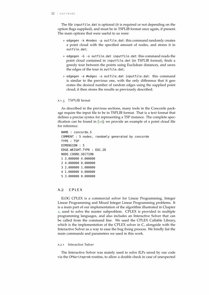
a.1.3 TSPLIB formatAs described in the previous sections, many tools in the Concorde pack-
age require the input file to be in TSPLIB format. That is a text format thatdefines a precise syntax for representing a TSP instance. The complete spec-ification can be found in [10]; we provide an example of a point cloud filefor reference.
NAME : concorde_5
COMMENT : 5 nodes, randomly generated by concorde
TYPE : TSP
DIMENSION : 5
EDGE_WEIGHT_TYPE : EUC_2D
NODE_COORD_SECTION
1 3.000000 4.000000
2 4.000000 0.000000
3 2.000000 1.000000
4 1.000000 4.000000
5 3.000000 0.000000
a.2 cplexILOG CPLEX is a commercial solver for Linear Programming, Integer
Linear Programming and Mixed Integer Linear Programming problems. Itis a main part of our implementation of the algorithm illustrated in Chapter2, used to solve the master subproblem. CPLEX is provided in multipleprogramming languages, and also includes an Interactive Solver that canbe called from the command line. We used the CPLEX Callable Library,which is the implementation of the CPLEX solver in C, alongside with theInteractive Solver as a way to ease the bug fixing process. We briefly list themain commands and parameters we used in this work.
a.2.1 Interactive SolverThe Interactive Solver was mainly used to solve ILPs saved by our code
via the CPXwriteprob routine, to allow a double check in case of unexpected

a.2 cplex 33
results from the application we were developing. The tool has proven in-valuable to find and solve troubles, especially some of them that were notapparent at all (usually related to numerical problems).
We provide a short list of the main commands we used in conjunctionwith the Interactive Solver.
• read <filename>: reads an ILP problem from the specified file.
• set [options]: allows to control various parameters that affect theexecution of CPLEX, for examples the ones that control the number ofnodes in the decisional tree or the amount of integer solution foundbefore exiting; more informations on the categories of parameters thatone can control are provided when the command is entered.
• mipopt: solve the current problem.
• display [options]: used to show the current solution of the ILP(display solution variables) or to access to the current parametersettings (display settings.
a.2.2 Callable LibraryThe Callable Library provides a C implementation of the CPLEX solver,
which is central for our goal, as already described multiple times. The mainroutines we used to implement our algorithm are listed below.
• CPXopenCPLEX(): creates the CPLEX environment that is needed forevery other call to it.
• CPXsetintparam() / CPXsetdblparam(): allows to control the param-eter settings that have been described previously in Chapters 3 and4.
• CPXcreateprob(): creates the (I)LP problem that will be initialized andsolved.
• CPXcopylp(): requires multiple arrays that describe the problem andloads them into it.
• CPXcopyctype(): similar to the previous one, it defines which variablesare integer and which one are not.
• CPXaddmipstarts(): allows to load one or more starting solutions tohopefully ease CPLEX’s computations.
• CPXmipopt(): optimizes the current problem.
• CPXgetx(): access the values of the decision variables after havingsolved the (I)LP.
• CPXgetobjval(): reads the objective function value corresponding tothe current solution.
• CPXgetnodecnt(): allows to know how many nodes of the decisionaltree were explored by the B&B algorithm CPLEX uses while solvingthe problem.
• CPXfreeprob(): frees the memory used by a problem.
• CPXcloseCPLEX(): closes the CPLEX evnironment after all the compu-tations have been completed.


B S O U R C E C O D E
b.1 main programb.1.1 tandem.h
1 #ifndef EDGE2 #define EDGE3
4 /* edge */5 typedef struct edge{6 double cost;7 int first_node;8 int second_node;9 } edge;
10
11 #endif12
13 int parseinput(int argc, char **argv);14 double get_cost(int *sol);15 int solve_master();16 int add_to_tabu_list(int *size, int **subtour);17 int *new_sec(int *size, int **subtour);18 static int setproblemdata (char **probname_p, int *numcols_p, int *numrows_p,19 int *objsen_p, double **obj_p, double **rhs_p,20 char **sense_p, int **matbeg_p, int **matcnt_p,21 int **matind_p, double **matval_p,22 double **lb_p, double **ub_p, char **ctype_p);23 int has_subtour(int *working_sol);24 int get_subtour(int *size, int **stour, int *working_sol);25 void print_current_status();26 void print_results();27 int evaluate_hamming(int *first, int *second);28 void free_and_null(char **ptr);29 void print_log_row(int iter, double m_cost, double s_cost, double best, int upd,30 double tar, double pctint, int hamm, int tabu_s, int cnodes, int maxnodes,31 double time_ela);
b.1.2 tandem.c
1 #include <stdio.h>2 #include <stdlib.h>3 #include <string.h>4 #include <time.h>5
6 #include "cplex.h"7
8 #include "tandem.h"9 #include "kruskal.h"
10
11 #define DEBUG 012
13 #if DEBUG14 #define PRINTVERBOSE(...) printf(__VA_ARGS__)15 #else16 #define PRINTVERBOSE(...) (void) 017 #endif18
19 #define PRINTERROR(...) fprintf(stderr, __VA_ARGS__)20
21 #define PRINTUSAGE() printf("Usage: tandem <edgefile> <tourfile> <max tabu size> \22 <iter limit> <time limit> <use slave?> <min percentual improvement> <intsollim = \23 1 ?> <use z RINS heuristic> <max node count binary> <max node count nonbinary>\n")24
35

36 source code
25
26 /* "global" variables */27
28 /* using slave? */29 int use_slave;30
31 /* slave at this iteration? */32 int slave_curr_iter;33
34 /* solution updated this iteration? */35 int sol_update;36
37 /* current target */38 double curr_target;39
40 double min_pct_impr;41
42 /* graph representation */43 int nnodes;44 int nedges;45
46 edge *edges;47 int **nodes;48 int *nodes_length;49
50 /* old and current master and slave */51 int *curr_master;52 int *curr_slave;53 int *old_master;54 int *old_slave;55
56 /* current solution */57 int *working_sol;58
59 /* tabu list */60 int **tabu;61 int num_nz;62 int tabu_size;63 int max_tabu_size;64
65 int tabu_change;66
67 /* best solution */68 int *best_sol;69
70 /* cplex env */71 CPXENVptr env;72 int cpxnodes;73 int maxnodecount_binary;74 int maxnodecount_nonbinary;75 int maxnodecount_actual;76 int intsollim;77
78 int iteration;79
80 /* sorted edge list */81 int *sorted_index;82
83 /* use z */84 int use_z;85
86 /* stopping conditions */87 int max_iter;88 double max_time;89 time_t start_time;90 /* end variables */91
92 /* parses the command line arguents */93 int parseinput(int argc, char **argv){94
95 PRINTVERBOSE("Parsing...\n");96
97 int status = 0;98 int a, b;99 int node1, node2;
100 double edgecost;101 int *temp;102 char *line = malloc(sizeof(char) * 100);103
104 if (argc < 11){
b.1 main program 37
105 PRINTERROR("Error: Not enough arguments.\n");106 PRINTUSAGE();107 exit(1);108 }109
110 FILE *edgefile = fopen ( argv[1], "r" );111 FILE *tourfile = fopen ( argv[2], "r" );112
113 if (edgefile == NULL || tourfile == NULL){114 PRINTERROR("Error: cannot open input files.\n");115 PRINTUSAGE();116 exit(1);117 }118
119 /* parse edgefile */120
121 /* leggo nnodes, nedges dalla prima riga */122 if (fgets(line,100,edgefile)==NULL){123 PRINTERROR("Error: cannot parse nnodes and nedges from edge file\n");124 exit(1);125 }126 nnodes = atoi(strtok (line, " "));127 nedges = atoi(strtok (NULL, " "));128
129 PRINTVERBOSE("%d nodes, %d edges\n", nnodes, nedges);130
131 edges = malloc(sizeof(edge)*nedges);132 nodes = malloc(sizeof(int*)*nnodes);133
134 nodes_length = malloc(sizeof(int)*nnodes);135
136 if (edges == NULL || nodes == NULL || nodes_length == NULL) {137 PRINTERROR("Error: out of memory while allocating data structures");138 exit(1);139 }140
141 for(a=0;a<nnodes;a++){142 nodes[a] = NULL;143 nodes_length[a] = 0;144 }145
146 for(a=0;a<nedges;a++){147
148 if (fgets(line,100,edgefile)==NULL){149 PRINTERROR("Error: not enough edges or edge file format incorrect\n");150 exit(1);151 }152
153 node1 = atoi(strtok(line, " "));154 node2 = atoi(strtok(NULL, " "));155 edgecost = atof(strtok(NULL, " "));156
157 if (node1>node2){158 int temp = node1;159 node1 = node2;160 node2 = temp;161 }162
163 edges[a].first_node = node1;164 edges[a].second_node = node2;165 edges[a].cost = edgecost;166
167 temp = realloc(nodes[node1], (nodes_length[node1]+1) * sizeof(int));168 if (temp == NULL){169 PRINTERROR("Error: failed to realloc memory in parseinput.\n");170 goto CLEANUP;171 }172 nodes_length[node1]++;173 nodes[node1] = temp;174 nodes[node1][nodes_length[node1]-1] = a;175
176 temp = realloc(nodes[node2], (nodes_length[node2]+1) * sizeof(int));177 if (temp == NULL){178 PRINTERROR("Error: failed to realloc memory in parseinput.\n");179 goto CLEANUP;180 }181 nodes_length[node2]++;182 nodes[node2] = temp;183 nodes[node2][nodes_length[node2]-1] = a;184
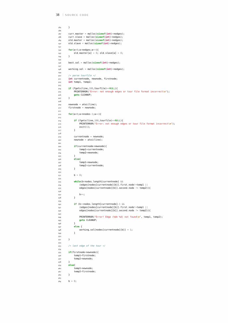
38 source code
185 }186
187 curr_master = malloc(sizeof(int)*nedges);188 curr_slave = malloc(sizeof(int)*nedges);189 old_master = malloc(sizeof(int)*nedges);190 old_slave = malloc(sizeof(int)*nedges);191
192 for(a=0;a<nedges;a++){193 old_master[a] = 0; old_slave[a] = 0;194 }195
196 best_sol = malloc(sizeof(int)*nedges);197
198 working_sol = malloc(sizeof(int)*nedges);199
200 /* parse tourfile */201 int currentnode, newnode, firstnode;202 int temp1, temp2;203
204 if (fgets(line,100,tourfile)==NULL){205 PRINTERROR("Error: not enough edges or tour file format incorrect\n");206 goto CLEANUP;207 }208
209 newnode = atoi(line);210 firstnode = newnode;211
212 for(a=0;a<nnodes-1;a++){213
214 if (fgets(line,100,tourfile)==NULL){215 PRINTERROR("Error: not enough edges or tour file format incorrect\n");216 exit(1);217 }218
219 currentnode = newnode;220 newnode = atoi(line);221
222 if(currentnode<newnode){223 temp1=currentnode;224 temp2=newnode;225 }226 else{227 temp1=newnode;228 temp2=currentnode;229 }230
231 b = 0;232
233 while(b<nodes_length[currentnode] &&234 (edges[nodes[currentnode][b]].first_node!=temp1 ||235 edges[nodes[currentnode][b]].second_node != temp2)){236
237 b++;238 }239
240 if (b==nodes_length[currentnode]-1 &&241 (edges[nodes[currentnode][b]].first_node!=temp1 ||242 edges[nodes[currentnode][b]].second_node != temp2)){243
244 PRINTERROR("Error! Edge (%dn %d) not found\n", temp1, temp2);245 goto CLEANUP;246 }247 else {248 working_sol[nodes[currentnode][b]] = 1;249 }250
251 }252
253 /* last edge of the tour */254
255 if(firstnode<newnode){256 temp1=firstnode;257 temp2=newnode;258 }259 else{260 temp1=newnode;261 temp2=firstnode;262 }263
264 b = 0;
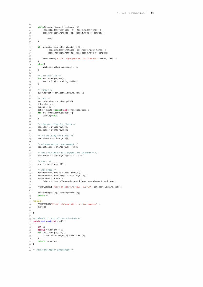
b.1 main program 39
265
266 while(b<nodes_length[firstnode] &&267 (edges[nodes[firstnode][b]].first_node!=temp1 ||268 edges[nodes[firstnode][b]].second_node != temp2)){269
270 b++;271 }272
273 if (b==nodes_length[firstnode]-1 &&274 (edges[nodes[firstnode][b]].first_node!=temp1 ||275 edges[nodes[firstnode][b]].second_node != temp2)){276
277 PRINTERROR("Error! Edge (%dn %d) not found\n", temp1, temp2);278 }279 else {280 working_sol[currentnode] = 1;281 }282
283 /* init best sol */284 for(a=0;a<nedges;a++){285 best_sol[a] = working_sol[a];286 }287
288 /* target */289 curr_target = get_cost(working_sol)-1;290
291 /* tabu */292 max_tabu_size = atoi(argv[3]);293 tabu_size = 0;294 num_nz = 0;295 tabu = malloc(sizeof(int*)*max_tabu_size);296 for(a=0;a<max_tabu_size;a++){297 tabu[a]=NULL;298 }299
300 /* time and iteration limits */301 max_iter = atoi(argv[4]);302 max_time = atof(argv[5]);303
304 /* are we using the slave? */305 use_slave = atoi(argv[6]);306
307 /* minimum percent improvement */308 min_pct_impr = atof(argv[7])/100;309
310 /* one solution or till otpimal one in master? */311 intsollim = atoi(argv[8])==1 ? 1 : 0;312
313 /* use z */314 use_z = atoi(argv[9]);315
316 /* max nodes */317 maxnodecount_binary = atoi(argv[10]);318 maxnodecount_nonbinary = atoi(argv[11]);319 maxnodecount_actual =320 (min_pct_impr)>0?maxnodecount_binary:maxnodecount_nonbinary;321
322 PRINTVERBOSE("Cost of starting tour: %.2f\n", get_cost(working_sol));323
324 fclose(edgefile); fclose(tourfile);325 return 0;326
327 CLEANUP:328 PRINTERROR("Error: cleanup still not implemented");329 exit(1);330
331 }332
333 /* calcola il costo di una soluzione */334 double get_cost(int *sol){335
336 int i;337 double to_return = 0;338 for(i=0;i<nedges;i++){339 to_return += edges[i].cost * sol[i];340 }341 return to_return;342 }343
344 /* solve the master subproblem */

40 source code
345
346 int solve_master(){347
348 /* cplex variables */349 char *probname = NULL;350 int numcols;351 int numrows;352 int objsen;353 double *obj = NULL;354 double *rhs = NULL;355 char *sense = NULL;356 int *matbeg = NULL;357 int *matcnt = NULL;358 int *matind = NULL;359 double *matval = NULL;360 double *lb = NULL;361 double *ub = NULL;362 char *ctype = NULL;363
364 int solstat;365 double *x = NULL;366
367 CPXLPptr lp = NULL;368
369 int status;370 int i, j;371 int cur_numrows, cur_numcols;372
373 /* initializes cplex data structures */374 status = setproblemdata (&probname, &numcols, &numrows, &objsen, &obj,375 &rhs, &sense, &matbeg, &matcnt, &matind, &matval,376 &lb, &ub, &ctype);377
378 if (status){379 PRINTERROR("Error: setproblemdata failed at iteration %d", iteration);380 exit(1);381 }382
383 x = malloc(sizeof(double)*numcols);384 if (x==NULL){385 PRINTERROR("Failed to allocate memory for solution array\n");386 exit(1);387 }388 for(i=0;i<nedges;i++){389 x[i]=0;390 }391
392 /* Create the problem. */393 lp = CPXcreateprob (env, &status, probname);394
395 if ( lp == NULL ) {396 PRINTERROR("Error: Failed to create LP.\n");397 goto TERMINATE;398 }399
400 /* Now copy the problem data into the lp */401 status = CPXcopylp (env, lp, numcols, numrows, objsen, obj, rhs,402 sense, matbeg, matcnt, matind, matval,403 lb, ub, NULL);404
405 if ( status ) {406 PRINTERROR("Failed to copy the problem data.\n");407 goto TERMINATE;408 }409
410 /* Now copy the ctype array */411 status = CPXcopyctype (env, lp, ctype);412 if ( status ) {413 PRINTERROR("Failed to copy ctype\n");414 goto TERMINATE;415 }416
417 /* add the appropriate mip start */418 if(use_z){419 int mcnt = 1;420 int nzcnt = nedges;421 int *beg = malloc(sizeof(int)*mcnt);422 int *effort = malloc(sizeof(int)*mcnt);423 beg[0] = 0;424 effort[0] = 4;

b.1 main program 41
425 int *varindices = malloc(sizeof(int)*nzcnt);426 double *values = malloc(sizeof(double)*nzcnt);427 for(i=0;i<nedges;i++){428 varindices[i] = i;429 values[i] = best_sol[i];430 }431 status = CPXaddmipstarts(env, lp, mcnt, nzcnt, beg, varindices, values, effort, NULL);432 }433
434 /* solve MIP */435 status = CPXmipopt (env, lp);436 if ( status ) {437 PRINTERROR("Error: Failed to optimize MIP. Status: %d\n", status);438 goto TERMINATE;439 }440 /* getting optimal assignment for decision variables */441 status = CPXgetx(env, lp, x, 0, CPXgetnumcols(env, lp)-2);442 int status2;443 double value = -1;444 status2 = CPXgetobjval(env, lp, &value);445 if ( status || (cpxnodes = CPXgetnodecnt(env, lp)) >= maxnodecount_actual ||446 value >= 50000 -2*nnodes -1) {447 if(status!=0 && status != 1217 /*&& value < 50000 -2*nnodes -1*/){448 PRINTERROR("Error: Failed to get decision variables.449 Status: %d\n", status);450 exit(1);451 } else {452 /* master is unfeasible; updating target and min_impr */453
454 if((curr_target / (1-min_pct_impr)) - curr_target <=1){455 print_results();456 printf("Error: Master is \"heuristically unfeasible\".457 Saving best tour in \"results.dat\"\n");458 printf("Elapsed time: %4.0f\n", ((double)time(NULL)) - start_time);459 exit(0);460 }461
462 slave_curr_iter = 0;463
464 curr_target = curr_target / (1-min_pct_impr);465 min_pct_impr /= 2;466 curr_target = curr_target * (1-min_pct_impr);467
468 if((curr_target / (1-min_pct_impr)) - curr_target <=1){469 status = CPXsetintparam (env, CPX_PARAM_NODELIM,470 maxnodecount_nonbinary);471 maxnodecount_actual = maxnodecount_nonbinary;472 }473
474 for(i=0;i<nedges;i++){475 old_master[i] = curr_master[i];476 curr_master[i] = 0;477 }478 }479 goto TERMINATE;480 }481
482 /* update working sol and master */483 for(i=0;i<numcols;i++){484 working_sol[i] = x[i]>0.5 ? 1 : 0;485 old_master[i] = curr_master[i];486 curr_master[i] = working_sol[i];487 }488
489 int *subtour;490 int size = 0;491
492 /* check if subtours are present */493 if(get_subtour(&size, &subtour, working_sol)){494 PRINTVERBOSE("Found subtour (%d): ", size);495 for(i=0;i<size;i++) PRINTVERBOSE("%d ", subtour[i]);496 PRINTVERBOSE("\n");497 add_to_tabu_list(&size, &subtour);498
499 free(subtour);500 } else {501 /* no subtour */502 if (get_cost(curr_master) <= curr_target){503
504 double new_target = (get_cost(curr_master) * (1-min_pct_impr));

42 source code
505 if (get_cost(curr_master) - new_target > 1){506 curr_target = new_target;507 } else {508 curr_target = get_cost(curr_master) - 1;509 if (maxnodecount_actual != maxnodecount_nonbinary){510 status = CPXsetintparam (env, CPX_PARAM_NODELIM,511 maxnodecount_nonbinary);512 maxnodecount_actual = maxnodecount_nonbinary;513 }514 }515 sol_update = 1;516 slave_curr_iter = 0;517
518 for(i=0;i<nedges;i++) best_sol[i] = curr_master[i];519 }520 }521 /* debug check, should never happen */522 if(!evaluate_hamming(curr_master, old_master)){523 printf("DEBUG: Master and previous one equals. Exiting...\n");524 CPXwriteprob(env, lp, "zerohamming.lp", NULL);525 exit(1);526 }527
528 PRINTVERBOSE("Master cost: %.2f\n", get_cost(curr_master));529
530 TERMINATE:531
532 /* free things */533
534 if ( lp != NULL ) {535 status = CPXfreeprob (env, &lp);536 if ( status ) {537 PRINTERROR("Error: CPXfreeprob failed, error code %d.\n", status);538 }539 }540 free_and_null ((char **) &probname);541 free_and_null ((char **) &obj);542 free_and_null ((char **) &rhs);543 free_and_null ((char **) &sense);544 free_and_null ((char **) &matbeg);545 free_and_null ((char **) &matcnt);546 free_and_null ((char **) &matind);547 free_and_null ((char **) &matval);548 free_and_null ((char **) &lb);549 free_and_null ((char **) &ub);550 free_and_null ((char **) &ctype);551 free(x);552
553 return (status);554
555 }556
557 /* adds constraint to tabu list */558 int add_to_tabu_list(int *size, int **subtour){559
560 int i, j, count;561
562 if(tabu_size<max_tabu_size){563 i = 0;564 while (tabu[i]!=NULL){565 i++;566 }567 tabu[i] = new_sec(size, subtour);568 tabu_size++;569 for(j=0;j<nedges;j++){570 num_nz += tabu[i][j];571 }572 } else {573 tabu_change = 1;574 for(j=0;j<nedges;j++){575 num_nz -= tabu[0][j];576 }577 free(tabu[0]);578 for(i=1;i<tabu_size;i++){579 tabu[i-1] = tabu[i];580 }581 tabu[tabu_size-1] = new_sec(size, subtour);582 for(j=0;j<nedges;j++){583 num_nz += tabu[tabu_size-1][j];584 }
b.1 main program 43
585 }586 }587
588 /* create SEC corresponding to passed subtour */589 int *new_sec(int *size, int **subtour){590
591 int i, j;592 int first, second;593 int *to_return = malloc(sizeof(int)*nedges);594 int *is_in_subtour=malloc(sizeof(int)*nnodes);595
596 if (to_return == NULL || is_in_subtour == NULL){597 PRINTERROR("Failed to allocate memory for solution array\n");598 exit(1);599 }600
601 for(i=0;i<nnodes;i++){602 is_in_subtour[i] = 0;603 }604
605 for(i=0;i<*size;i++){606 is_in_subtour[(*subtour)[i]] = 1607 }608
609 for(i=0;i<nedges;i++){610 if((is_in_subtour[edges[i].first_node] &&611 !is_in_subtour[edges[i].second_node]) ||612 (is_in_subtour[edges[i].second_node] &&613 !is_in_subtour[edges[i].first_node])){614 to_return[i] = 1;615 } else to_return[i] = 0;616 }617 free(is_in_subtour);618
619 return to_return;620 }621
622
623 /* initialize cplex arrays */624 static int setproblemdata (char **probname_p, int *numcols_p, int *numrows_p,625 int *objsen_p, double **obj_p, double **rhs_p,626 char **sense_p, int **matbeg_p, int **matcnt_p,627 int **matind_p, double **matval_p,628 double **lb_p, double **ub_p, char **ctype_p){629
630 int i, j;631 cell *iter;632
633 char *zprobname = NULL; /* Problem name <= 16 characters */634 double *zobj = NULL;635 double *zrhs = NULL;636 char *zsense = NULL;637 int *zmatbeg = NULL;638 int *zmatcnt = NULL;639 int *zmatind = NULL;640 double *zmatval = NULL;641 double *zlb = NULL;642 double *zub = NULL;643 char *zctype = NULL;644 int status = 0;645
646 int numcols = nedges + use_z;647 int numrows = nnodes + 1 + tabu_size;648
649 int numnz = 3*numcols + num_nz + use_z;650
651 zprobname = (char *) malloc (16 * sizeof(char));652 zobj = (double *) malloc (numcols * sizeof(double));653 zrhs = (double *) malloc (numrows * sizeof(double));654 zsense = (char *) malloc (numrows * sizeof(char));655 zmatbeg = (int *) malloc (numcols * sizeof(int));656 zmatcnt = (int *) malloc (numcols * sizeof(int));657 zmatind = (int *) malloc (numnz * sizeof(int));658 zmatval = (double *) malloc (numnz * sizeof(double));659 zlb = (double *) malloc (numcols * sizeof(double));660 zub = (double *) malloc (numcols * sizeof(double));661 zctype = (char *) malloc (numcols * sizeof(char));662
663 if ( zprobname == NULL || zobj == NULL ||664 zrhs == NULL || zsense == NULL ||
44 source code
665 zmatbeg == NULL || zmatcnt == NULL ||666 zmatind == NULL || zmatval == NULL ||667 zlb == NULL || zub == NULL ||668 zctype == NULL ) {669 status = 1;670 goto TERMINATE;671 }672
673 sprintf(zprobname, "Master_%d", iteration);674
675 /* setting zobj */676 for(i=0;i<numcols-use_z;i++){677 if(working_sol[i]) zobj[i] = -1; else zobj[i] = 1;678 }679 /* z */680 if (use_z) zobj[numcols-1] = 50000;681
682 int count;683 /* setting other things */684 for(i=0;i<numcols-use_z;i++){685 count = 0;686 for(j=0;j<tabu_size;j++){687 count+=tabu[j][i];688 }689 zmatcnt[i]=3 + count;690 if(i==0){691 zmatbeg[i]=0;692 } else {693 zmatbeg[i]=zmatbeg[i-1]+zmatcnt[i-1];694 }695
696 zmatind[zmatbeg[i]]=edges[i].first_node;697 zmatind[zmatbeg[i]+1]=edges[i].second_node;698 zmatind[zmatbeg[i]+2]=nnodes;699
700 zmatval[zmatbeg[i]]=1;701 zmatval[zmatbeg[i]+1]=1;702 zmatval[zmatbeg[i]+2]=edges[i].cost;703 /* tabu */704 count = 0;705 for(j=0;j<tabu_size;j++){706 if(tabu[j][i] == 1){707 zmatind[zmatbeg[i]+3+count]=nnodes+1+j;708 zmatval[zmatbeg[i]+3+count]=1;709 count++;710 }711 }712
713 /* binary integer vars */714 zlb[i]=0;715 zub[i]=1;716 zctype[i]=’I’;717 }718 /* z */719 if(use_z){720 zmatcnt[numcols-1] = 1;721 zmatbeg[numcols-1] = zmatbeg[numcols-2] + zmatcnt[numcols-2];722 zmatind[zmatbeg[numcols-1]] = nnodes;723 zmatval[zmatbeg[numcols-1]] = -1;724 zlb[numcols-1] = 0;725 zub[numcols-1] = CPX_INFBOUND;726 zctype[numcols-1] = ’I’;727 }728
729 /* rhs’s */730 for(i=0;i<nnodes;i++){731 zsense[i]=’E’;732 zrhs[i]=2;733 }734 zsense[nnodes]=’L’;735 zrhs[nnodes]=curr_target;736
737 for(i=nnodes+1;i<numrows;i++){738 zsense[i]=’G’;739 zrhs[i]=2;740 }741
742 TERMINATE:743 if ( status ) {744 free_and_null ((char **) &zprobname);

b.1 main program 45
745 free_and_null ((char **) &zobj);746 free_and_null ((char **) &zrhs);747 free_and_null ((char **) &zsense);748 free_and_null ((char **) &zmatbeg);749 free_and_null ((char **) &zmatcnt);750 free_and_null ((char **) &zmatind);751 free_and_null ((char **) &zmatval);752 free_and_null ((char **) &zlb);753 free_and_null ((char **) &zub);754 free_and_null ((char **) &zctype);755 }756 else {757 *numcols_p = numcols;758 *numrows_p = numrows;759 *objsen_p = CPX_MIN; /* The problem is minimization */760
761 *probname_p = zprobname;762 *obj_p = zobj;763 *rhs_p = zrhs;764 *sense_p = zsense;765 *matbeg_p = zmatbeg;766 *matcnt_p = zmatcnt;767 *matind_p = zmatind;768 *matval_p = zmatval;769 *lb_p = zlb;770 *ub_p = zub;771 *ctype_p = zctype;772 }773 return (status);774
775 }776
777 /* solves the slave subproblem */778 int solve_slave(){779
780 int i,j;781
782 if(use_slave && slave_curr_iter){783
784 int *sorted_after_m = malloc(sizeof(int)*(nedges-nodes_length[nnodes-1]));785
786 int count = 0;787 for(i=0;i<nedges;i++){788 if(working_sol[sorted_index[i]] &&789 edges[sorted_index[i]].second_node!=nnodes-1){790 sorted_after_m[count] = sorted_index[i];791 count++;792 }793 }794 for(i=0;i<nedges;i++){795 if(!(working_sol[sorted_index[i]]) &&796 edges[sorted_index[i]].second_node!=nnodes-1){797 sorted_after_m[count] = sorted_index[i];798 count++;799 }800 }801
802 int *tree = NULL;803
804 kruskal(nedges, nnodes-1, edges, sorted_after_m, &tree);805
806 int best, secbest;807
808 if (edges[nodes[nnodes-1][0]].cost > edges[nodes[nnodes-1][1]].cost){809 best = nodes[nnodes-1][1]; secbest = nodes[nnodes-1][0];810 } else {811 best = nodes[nnodes-1][0]; secbest = nodes[nnodes-1][1];812 }813
814 for(i=2;i<nodes_length[nnodes-1];i++){815 if (edges[nodes[nnodes-1][i]].cost < best){816 secbest = best;817 best = nodes[nnodes-1][i];818 } else if (edges[nodes[nnodes-1][i]].cost < best){819 secbest = nodes[nnodes-1][i];820 }821 }822
823 tree[best] = 1;824 tree[secbest] = 1;

46 source code
825
826 for(i=0;i<nedges;i++){827 working_sol[i] = tree[i];828 old_slave[i] = curr_slave[i];829 curr_slave[i] = tree[i];830 }831
832 free(sorted_after_m);833 free(tree);834
835 if((!has_subtour(curr_slave)) && get_cost(curr_slave) <= curr_target){836
837 double new_target = (get_cost(curr_slave) * (1-min_pct_impr));838 if (get_cost(curr_slave) - new_target > 1){839 curr_target = new_target;840 } else {841 curr_target = get_cost(curr_slave) - 1;842 if (maxnodecount_actual != maxnodecount_nonbinary){843 int status = CPXsetintparam (env, CPX_PARAM_NODELIM,844 maxnodecount_nonbinary);845 maxnodecount_actual = maxnodecount_nonbinary;846 }847 }848 sol_update = 1;849
850 for(i=0;i<nedges;i++) best_sol[i] = curr_slave[i];851 }852
853 } else {854 PRINTVERBOSE("DEBUG: Slave not executed at iteration %d\n", iteration);855 for(i=0;i<nedges;i++){856 curr_slave[i] = curr_master[i];857 }858 }859 }860
861 /* wrapper */862 int has_subtour(int *working_sol){863 int *sub = NULL;864 int a = 0;865
866 int to_return = get_subtour(&a, &sub, working_sol);867
868 free(sub);869 return to_return;870 }871
872 /* returns 1 if a subtour is found, 0 otherwise*/873 int get_subtour(int *size, int **stour, int *working_sol){874
875 int *subtour = malloc (sizeof(int)*nnodes);876 int *shortest_subtour = malloc (sizeof(int)*nnodes);877 int *visited = malloc (sizeof(int)*nnodes);878
879 int prev, cur, next, cur_edge, i, j, k, start;880
881 int len_shortest_subtour = nnodes;882
883 for(i=0;i<nnodes;i++){884 visited[i] = 0;885 }886
887 while(1){888
889 for(i=0;i<nnodes;i++){890 subtour[i] = -1;891 }892
893 for(j=0;j<nnodes;j++){894 if(!visited[j]){895 cur = j;896 visited[cur] = 1;897
898 for(k=0;k<nodes_length[cur];k++){899 if(working_sol[nodes[cur][k]] &&900 (!visited[edges[nodes[cur][k]].first_node] ||901 !visited[edges[nodes[cur][k]].second_node])){902
903 if(cur == edges[nodes[cur][k]].first_node){904 next = edges[nodes[cur][k]].second_node;

b.1 main program 47
905 } else {906 next = edges[nodes[cur][k]].first_node;907 }908 cur_edge = nodes[cur][k];909 break;910 }911 }912 break;913 }914 }915 if (j == nnodes) break;916
917 i = 0;918 subtour[i++] = cur;919
920 while(1){921 prev = cur;922 cur = next;923
924 j = 0;925 while(j<nnodes && subtour[j]!=-1 && subtour[j]!=cur){926 j++;927 }928 if (j==nnodes-1 && subtour[j]!=cur){929 free(subtour);930 free(visited);931 return 0;932 }933
934 if (subtour[j]==cur){935
936 break;937 }938
939 subtour[i++] = cur;940 visited[cur] = 1;941
942 k = 0;943 while(k<nodes_length[cur] && !(working_sol[nodes[cur][k]]944 && edges[nodes[cur][k]].first_node != prev945 && edges[nodes[cur][k]].second_node != prev )){946
947 k++;948 }949 if (k==nodes_length[cur]) {950 free(subtour);951 free(visited);952 return 2;953 }954
955
956 if (edges[nodes[cur][k]].first_node == cur){957 next = edges[nodes[cur][k]].second_node;958 } else{959 next = edges[nodes[cur][k]].first_node;960 }961 }962
963 if(i < len_shortest_subtour){964 len_shortest_subtour = i;965
966 for(j=0;j<nnodes;j++){967 shortest_subtour[j] = subtour[j];968 subtour[j] = -1;969 }970 }971 }972
973 i = 0;974 while(shortest_subtour[i]!=-1){975 i++;976 }977 int *temp = realloc(shortest_subtour, sizeof(int)*i);978 if(temp == NULL){979 PRINTERROR("Error: failed to realloc memory in subtour detection\n");980 exit(1);981 } else {982 *stour = temp;983 *size = i;984 free(subtour);

48 source code
985 free(visited);986 PRINTVERBOSE("Size of subtour: %d\n", i);987 return 1;988 }989 }990
991 /* debug functions, prints lots of infos about the status of the algorithm */992 void print_current_status(){993 int i, j;994
995 for(i=0;i<nedges;i++){996 PRINTVERBOSE("%d: %d, %d, %.2f, %d\n", i,997 edges[i].first_node, edges[i].second_node,998 edges[i].cost, working_sol[i]);999 }
1000
1001 PRINTVERBOSE("----------------------------------------\n");1002
1003 for(i=0;i<nnodes;i++){1004 PRINTVERBOSE("Edges incident on %d (%d): ", i, nodes_length[i]);1005 for(j=0;j<nodes_length[i];j++){1006 PRINTVERBOSE("(%d %d)", edges[nodes[i][j]].first_node,1007 edges[nodes[i][j]].second_node);1008 }1009 PRINTVERBOSE("\n");1010 }1011 }1012
1013 /* prints final tour */1014 void print_results(){1015
1016 FILE *out = fopen ("results.dat","w");1017
1018 int i, j, k, cur, prev, next;1019
1020 cur = 0;1021 for(i=0;i<nodes_length[0];i++){1022 if(best_sol[nodes[0][i]]){1023 next = nodes[0][i];1024 }1025 }1026
1027 fprintf(out, "%d\n", cur);1028
1029 for(i=0;i<nnodes-1;i++){1030 prev = cur;1031 cur = next;1032
1033 fprintf(out, "%d\n", cur);1034
1035 /* trovo il nuovo next */1036 k = 0;1037 while(k<nodes_length[cur] && !(best_sol[nodes[cur][k]]1038 && edges[nodes[cur][k]].first_node != prev1039 && edges[nodes[cur][k]].second_node != prev )){1040
1041 k++;1042 }1043 /* aggiorno next */1044
1045 if (edges[nodes[cur][k]].first_node == cur){1046 next = edges[nodes[cur][k]].second_node;1047 } else{1048 next = edges[nodes[cur][k]].first_node;1049 }1050 }1051 fclose(out);1052 }1053
1054 /* evaluates hamming distance between two solutions */1055 int evaluate_hamming(int *first, int *second){1056
1057 int i, to_return;1058 to_return = 0;1059 for(i=0;i<nedges;i++){1060 if(first[i] != second[i]){1061 to_return++;1062 }1063 }1064 return to_return;

b.1 main program 49
1065
1066 }1067
1068 int main(int argc, char **argv){1069
1070 iteration = 0;1071 tabu_change = 0;1072 sol_update = 0;1073 cpxnodes = 0;1074 slave_curr_iter = 1;1075
1076 int status;1077 env = CPXopenCPLEX(&status);1078 if(status){1079 PRINTERROR("Error: failed to initialize CPLEX environment\n");1080 exit(1);1081 }1082
1083 parseinput(argc, argv);1084
1085
1086 if(use_z){1087 status = CPXsetdblparam (env, CPX_PARAM_OBJDIF, 50000 - 2*nnodes -1);1088 status = CPXsetintparam (env, CPX_PARAM_RINSHEUR, 50);1089 intsollim = 0;1090 } else if (intsollim){1091 status = CPXsetintparam (env, CPX_PARAM_INTSOLLIM, 1);1092 }1093 status = CPXsetintparam (env, CPX_PARAM_NODELIM, maxnodecount_actual);1094
1095 if ( use_slave ){1096 kruskal_setup(nedges, nnodes, edges, &sorted_index);1097 } else {1098 sorted_index = NULL;1099 }1100
1101 if(DEBUG>0) print_current_status();1102
1103 PRINTVERBOSE("Initial tour cost is: %.2f\n", get_cost(working_sol));1104
1105 if (!DEBUG){1106 printf("Initial graph: %d nodes, %d edges\n", nnodes, nedges);1107 printf("Initial tour cost: %.2f\n", get_cost(working_sol));1108 printf("Starting minimum percent improvement: %3.2f\n", min_pct_impr);1109 printf("Iteration limit: %d, Time limit: %.0fs\n", max_iter, max_time);1110 printf("Slave is %s; CPLEX_PARAM_INTSOLLIM is set to %s\n",1111 use_slave?"ON":"OFF", intsollim?"1":"default");1112 }1113
1114 start_time = time(NULL);1115
1116 while(iteration<max_iter && ((double)time(NULL)) - start_time<max_time){1117 iteration++;1118 tabu_change = 0;1119 sol_update = 0;1120 cpxnodes = 0;1121 slave_curr_iter = 1;1122
1123 if (!DEBUG && iteration%15==1){1124 printf("Iter Master Slave Best Target PctImp Hamm");1125 printf(" TabuSiz Nodes NodLim Elaps(s)\n");1126 }1127
1128
1129 PRINTVERBOSE("\nIteration %d started.\n", iteration);1130
1131 PRINTVERBOSE("Calling solve_master...\n");1132 solve_master();1133 PRINTVERBOSE("solve_master done!\n");1134
1135 if(DEBUG>1) print_current_status();1136
1137 PRINTVERBOSE("Calling solve_slave...\n");1138 solve_slave();1139 PRINTVERBOSE("solve_slave done!\n");1140
1141 if (DEBUG>1) print_current_status();1142
1143 PRINTVERBOSE("Iteration %d done\n", iteration);1144 PRINTVERBOSE("Cost of current solution: %.2f\n", get_cost(working_sol));
50 source code
1145
1146 if (!DEBUG) print_log_row(iteration,1147 get_cost(curr_master), get_cost(curr_slave), get_cost(best_sol),1148 sol_update, curr_target, min_pct_impr,1149 evaluate_hamming(curr_master, curr_slave),1150 tabu_size, cpxnodes, maxnodecount_actual,1151 ((double)time(NULL)) - start_time);1152 }1153
1154 PRINTVERBOSE("\nStopping condition reached.\n");1155 if(1){1156 PRINTVERBOSE("Found a tour of cost less than the target\n");1157 PRINTVERBOSE("Saving the tour in \"results.dat\"\n");1158 print_results();1159 }1160 PRINTVERBOSE("Exiting...\n");1161
1162 CPXcloseCPLEX(&env);1163 }1164
1165 void print_log_row(int iter, double m_cost, double s_cost, double best, int upd,1166 double tar, double pctint, int hamm, int tabu_s, int cnodes, int maxnodes,1167 double time_ela){1168
1169 if(!m_cost){1170 printf("%3d: %s %s %7.1f%s %7.1f %3.2f %s",1171 iteration, "-", "-", best, upd?"*":" ",tar, pctint, " -");1172 printf("%2d %4d %4d %4.0f\n", tabu_size, cnodes, maxnodes,1173 time_ela);1174 }1175
1176 else if (m_cost == s_cost){1177 printf("%3d: %7.1f %s %7.1f%s %7.1f %3.2f %s",1178 iteration, m_cost, "-", best, upd?"*":" ",tar, pctint, " -");1179 printf("%2d %4d %4d %4.0f\n", tabu_size, cnodes, maxnodes,1180 time_ela);1181 }1182
1183 else{1184 printf("%3d: %7.1f %7.1f %7.1f%s %7.1f %3.2f %5d",1185 iteration, m_cost, s_cost, best, upd?"*":" ",tar, pctint, hamm);1186 printf("%2d %4d %4d %4.0f\n", tabu_size, cnodes, maxnodes,1187 time_ela);1188 }1189 }1190
1191
1192 void free_and_null(char **ptr){1193 if (*ptr!=NULL){1194 free(*ptr);1195 *ptr = NULL;1196 }1197 }
b.2 kruskal implementationb.2.1 kruskal.h
1 #ifndef EDGE2 #define EDGE3
4 /* lato del grafo */5 typedef struct edge{6 double cost; //costo del lato7 int first_node; //primo nodo8 int second_node; //secondo nodo9 } edge;
10
11 #endif12
13 typedef struct data{14 double cost;15 int index;

b.2 kruskal implementation 51
16 } data;17
18 int quick_sort(data *arr, int elements);19 int kruskal_setup(int nedges, int nnodes, edge *edges, int **sorted_index);20 int kruskal(int nedges, int nnodes, edge *edges, int *sorted_index, int **tree);
b.2.2 kruskal.c
1 #include <stdio.h>2 #include <stdlib.h>3 #include "kruskal.h"4
5 #define MAX_LEVELS 10006
7 int quick_sort(data *arr, int elements) {8
9 data piv;10 int beg[MAX_LEVELS], end[MAX_LEVELS], i=0, L, R ;11
12 beg[0]=0; end[0]=elements;13 while (i>=0) {14 L=beg[i]; R=end[i]-1;15 if (L<R) {16 piv=arr[L]; if (i==MAX_LEVELS-1) return 1;17 while (L<R) {18 while (arr[R].cost>=piv.cost && L<R) R--; if (L<R) arr[L++]=arr[R];19 while (arr[L].cost<=piv.cost && L<R) L++; if (L<R) arr[R--]=arr[L];20 }21 arr[L]=piv; beg[i+1]=L+1; end[i+1]=end[i]; end[i++]=L;22 }23 else {24 i--;25 }26 }27 return 0;28 }29
30 /* sorts the list, basically just a mergesort */31 int kruskal_setup(int nedges, int nnodes, edge *edges, int **sorted_index){32
33 data *temp_list = malloc(sizeof(data)*nedges);34
35 int i;36 for(i=0;i<nedges;i++){37 temp_list[i].cost = edges[i].cost;38 temp_list[i].index = i;39 }40
41 int status = quick_sort(&temp_list[0], nedges);42 if(status){43 printf("Error: quicksort failed\n");44 exit(1);45 }46
47 *sorted_index = malloc(sizeof(int)*nedges);48 for(i=0;i<nedges;i++){49 (*sorted_index)[i]=temp_list[i].index;50 }51 free(temp_list);52 return 0;53
54 }55
56 int kruskal(int nedges, int nnodes, edge *edges, int *sorted_index, int **tree){57
58 int i;59
60 int *prev = malloc(sizeof(int)*nnodes);61 *tree = malloc(sizeof(int)*nedges);62
63 for(i=0;i<nnodes;i++){64 prev[i]=-1;65 }66
67 for(i=0;i<nedges;i++){68 (*tree)[i]=0;

52 source code
69 }70
71 int head = 0;72 int temp;73 int node1, node2;74 int selected = 0;75
76 while (selected!=nnodes-1){77
78 temp = sorted_index[head];79 head++;80
81 node1 = edges[temp].first_node;82 node2 = edges[temp].second_node;83
84 while(prev[node1]>-1){85 node1 = prev[node1];86 }87
88 while(prev[node2]>-1){89 node2 = prev[node2];90 }91
92 if(node1!=node2){93 (*tree)[temp]=1;94 prev[node2]=node1;95 selected++;96 }97 }98 free(prev);99 }
b.3 instance generationb.3.1 script.sh
1 #!/bin/bash2
3 #$1=nnods, $2=nedges, $3=outfile4
5 ./edgegen -k $1 -p ${3}_pointcloud_nontsp.dat6
7 rm -f ${3}_pointcloud_tsp.dat ${3}_pointcloud_numbered.dat8 awk ’{printf "%d %s\n", NR-1, $0}’ < ${3}_pointcloud_nontsp.dat9 >> ${3}_pointcloud_numbered.dat
10 echo "NAME : concorde_$1" >> ${3}_pointcloud_tsp.dat11 echo "COMMENT : $1 nodes, randomly generated by concorde" >> ${3}_pointcloud_tsp.dat12 echo "TYPE : TSP" >> ${3}_pointcloud_tsp.dat13 echo "DIMENSION : $1" >> ${3}_pointcloud_tsp.dat14 echo "EDGE_WEIGHT_TYPE : EUC_2D" >> ${3}_pointcloud_tsp.dat15 echo "NODE_COORD_SECTION" >> ${3}_pointcloud_tsp.dat16 tail -n +2 ${3}_pointcloud_numbered.dat >> ${3}_pointcloud_tsp.dat17
18 ./edgegen -G -o ${3}_tour_toconvert.dat ${3}_pointcloud_tsp.dat19 ./converter ${3}_tour_toconvert.dat ${3}_tourfile.dat20 ./edgegen -e $2 -o ${3}_randomedges_tomerge.dat ${3}_pointcloud_tsp.dat21 ./merger ${3}_tour_toconvert.dat ${3}_randomedges_tomerge.dat $2 ${3}_edgefile.dat22 rm ${3}_tour_toconvert.dat ${3}_randomedges_tomerge.dat ${3}_pointcloud_nontsp.dat23 ${3}_pointcloud_numbered.dat24 exit
b.3.2 converter.c
1 #include <stdio.h>2 #include <stdlib.h>3
4
5
6 int main(int *argc, char **argv){

b.3 instance generation 53
7
8 FILE *in = fopen(argv[1], "r");9 int nnodes, nedges;
10
11 fscanf(in, "%d", &nnodes);12 fscanf(in, "%d", &nedges);13
14 int *edges = malloc(sizeof(int)*2*nedges);15
16 int i, j, dummy;17
18 for(i=0;i<nedges;i++){19
20 fscanf(in, "%d", &edges[2*i]);21 fscanf(in, "%d", &edges[2*i+1]);22 fscanf(in, "%d", &dummy);23 }24
25 fclose(in);26 FILE *out = fopen(argv[2], "w");27
28 int cur, prev, next;29
30 fprintf(out, "%d\n", edges[0]);31 cur = edges[0];32 next = edges [1];33 //printf("%d %d\n", cur, next);34
35 for(i=0;i<nedges-1;i++){36
37 prev=cur;38 cur=next;39 fprintf(out, "%d\n", cur);40
41 for(j=0;j<nedges;j++){42
43 if(edges[2*j]==cur && edges[2*j+1]!=prev) break;44 if(edges[2*j+1]==cur && edges[2*j]!=prev) break;45 }46
47 next = edges[2*j]==cur ? edges[2*j+1] : edges[2*j];48 }49 close(out);50
51 }
b.3.3 merger.c
1 #include <stdio.h>2 #include <stdlib.h>3
4 /* argv[1]="tour file", argv[2]=random file, argv[3]=out file*/5 int main(int *argc, char **argv){6
7 int max_edges = atoi(argv[3]);8
9 FILE *in = fopen(argv[1], "r");10 int nnodes, nedges;11
12 fscanf(in, "%d", &nnodes);13 fscanf(in, "%d", &nedges);14
15 int *edges = malloc(sizeof(int)*2*nedges);16 int *weights = malloc(sizeof(int)*nedges);17
18 int i, j, dummy;19
20 for(i=0;i<nedges;i++){21
22 fscanf(in, "%d", &edges[2*i]);23 fscanf(in, "%d", &edges[2*i+1]);24 fscanf(in, "%d", &weights[i]);25 }26
27 fclose(in);28

54 source code
29 FILE *in2 = fopen(argv[2], "r");30 int nnodes2, nedges2, nondupedges;31
32 fscanf(in2, "%d", &nnodes2);33 fscanf(in2, "%d", &nedges2);34
35 nondupedges=0;36
37 int *edges2 = malloc(sizeof(int)*2*nedges2);38 int *weights2 = malloc(sizeof(int)*nedges2);39
40 int first, second, weight, duplicate;41 for(i=0;i<nedges2;i++){42 duplicate = 0;43
44 fscanf(in, "%d", &first);45 fscanf(in, "%d", &second);46 fscanf(in, "%d", &weight);47
48 /* elimino duplicati */49 for(j=0;j<nedges;j++){50 if(first==edges[2*j] && second==edges[2*j+1]) {duplicate = 1;51 break;52 }53 }54
55 if (duplicate == 1) { continue;}56 else{57 edges2[2*nondupedges]=first;58 edges2[2*nondupedges+1]=second;59 weights2[nondupedges]=weight;60 nondupedges++;61 }62 if (nondupedges + nedges == max_edges) break;63 }64
65 fclose(in2);66
67 FILE *out = fopen (argv[4], "w");68
69 fprintf(out, "%d %d\n", nnodes, nedges + nondupedges);70
71 for(i=0;i<nedges;i++) fprintf(out, "%d %d %d\n", edges[i*2],72 edges[i*2+1], weights[i]);73
74 for(i=0;i<nondupedges;i++) fprintf(out, "%d %d %d\n", edges2[i*2],75 edges2[i*2+1], weights2[i]);76 fclose(out);77
78 }

B I B L I O G R A P H Y[1] David L. Applegate, Robert E. Bixby, Vasek Chvátal, and William
J. Cook. The Traveling Salesman Problem. Ed. by Princeton UniversityPress. (Winner of the 2007 Lanchester Prize, INFORMS). 2006.
[2] Concorde documentation. url: http://www.tsp.gatech.edu/concorde/DOC/concorde_org.html.
[3] Concorde website. url: http://www.tsp.gatech.edu/concorde.html.
[4] M. Fischetti. Lezioni di Ricerca Operativa. 1999.
[5] M. Fischetti, F. Glover, and A. Lodi. “The Feasibility Pump”. url:http://www.dei.unipd.it/~fisch/papers/feasibility_pump.pdf.
[6] G. Gutin and A.P. Punnen. The Traveling Salesman Problem and Its Vari-ations. Ed. by Springer. 2002.
[7] ILOG CPLEX documentation. url: http://pic.dhe.ibm.com/infocenter/cosinfoc/v12r5/index.jsp.
[8] M. Jünger, G. Reinelt, and G. Rinaldi. “The Traveling Salesman Prob-lem: A Computational Study”. In: Handbooks in Operations Reseach andManagement Science 7 (). Ed. by Elsevier Science B.V., pp. 225–330.
[9] D.B. Shmoys, J.K. Lenstra, A.H.G. Rinnooy Kan, and E.L. Lawler. TheTraveling Salesman Problem. Ed. by John Wiley & Sons. 1985.
[10] TSPLIB Specifications. url: http://comopt.ifi.uni-heidelberg.de/software/TSPLIB95/DOC.PS.
[11] Wikipedia. Travelling Salesman Problem. url: http://en.wikipedia.org/wiki/Travelling_salesman_problem.
55