An integral equation solution for the steady-state

current at a periodic array of surface microelectrodes

S.K. Lucas, School of Mathematics, University of South Australia,The Levels SA 5095, AUSTRALIA

H.A. Stone, Division of Applied Sciences, Harvard University, Cam-bridge MA 02138, U.S.A.

R. Sipcic, Department of Mathematics, Massachusetts Institute ofTechnology, Cambridge MA 02139, U.S.A.

Submitted September 1995, Revised July 1996,to SIAM Journal on Applied Mathematics

Abstract

An integral equation approach is developed for the problem of determiningthe steady-state current to a periodic array of microelectrodes imbedded in anotherwise insulating plane. The formulation accounts for both surface electrodeand bulk fluid reactions, and evaluates the Green’s functions for periodic systemsusing convergence acceleration techniques. Numerical results are presented fordisc-shaped microelectrodes at the center of rectangular periodic cells for a largerange of dimensionless surface and bulk reaction rates and periodic cell sizes.

Keywords:

electrochemistry, reaction-diffusion, boundary integral method, microelectrode arrays

Subject Classifications:

92E20 - Chemistry, Reactions65R20 - Numerical analysis, Integral equations65B99 - Acceleration of convergence, Other

Abbreviated title:

Current at an array of microelectrodes

1

1 Introduction

Mass transport coupling diffusion, surface and/or bulk chemical reactions, and speciesmigration in external fields occurs in a wide variety of physical situations, includingelectrochemistry, catalysis, corrosion, colloidal suspensions, and protein binding. Suchtransport processes are frequently controlled by surface chemical reactions or by chargedistributed along the surfaces bounding the fluid. In general, the bounding surfaces areheterogeneous and so surface properties (e.g. reactivity) vary. For example, electrochem-ical devices consisting of arrays of microelectrodes (Wightman and Wipf [35], Mallouk[19]) or catalysis along heterogeneous surfaces (Kuan et al. [16, 17]) have in commonthe geometric feature that surface chemical reactions occur on many distributed regions,or patches, on an otherwise unreactive substrate. Although mass transfer to an isolatedsurface patch has been studied for a variety of surface geometries (e.g. strips, hemi-spheres, discs, and rings), the case of multiple active surface sites has received much lessattention. This paper addresses this question by studying reaction-diffusion problemsin a stationary fluid bounded by a plane that is covered by a periodic array of circularreactive sites.

The electrochemical literature contains many studies of the current at an electrodeof various given shapes. The small size of microelectrodes typically leads to situationswhere transients are short-lived and so the accompanying mass transport may be treatedas steady state. Isolated microelectrodes in the shape of hemispheres (Oldham and Zoski[23]), discs (Aoki et al. [2], Bond et al. [6], Phillips [24, 25], Bender and Stone [5]) andrings (Fleischmann et al. [9, 10], Szabo [33], Phillips and Stone [27]) have been analyzedmost frequently, mostly for the case of bulk diffusion with surface chemical reaction (theLaplace equation), but also for bulk diffusion with surface chemical reaction and bulkspecies regeneration by chemical reaction (the modified Helmholtz equation).

Recent electrochemical applications utilize microelectrode arrays (Wightman andWipf [35]). In general, it is of interest to determine an effective rate constant for theheterogeneous surface which depends on both the reactivity of active sites as well as theirsurface coverage. Theoretical analysis of such arrays must treat the interaction of thedifferent surface reactive sites and, perhaps not surprisingly, theoretical analyses havebeen limited to the case of small fractional coverages of a finite surface (Phillips [26])and numerical results for a small number of electrodes on an infinite surface (Fransaeret al. [11]). Included in [26] are several references to problems dealing with microelec-trode arrays of infinite extent, including studies by Reller et al. [30] and Scharifker [32],who investigate time-dependent currents, though since diffusion with no regenerationwithin the fluid is considered, the steady state result is zero current. In addition, in[30] and [32], a periodic array geometry is approximated by solving instead the prob-lem of a disc electrode surrounded by an insulating annulus. We also note that masstransport problems related to the present investigation of multiple reactive surface sitesnaturally arise in the modelling of catalytic surfaces (Kuan et al. [16, 17]), the doublelayer forces between surfaces with a heterogeneous charge distribution (Miklavic et al.

[20]), multi-particle Ostwald ripening (Voorhees and Glicksman [34]), and protein bind-ing (Balgi et al. [3]). Related mathematical formulations also arise in studies of theeffective conductivity of a suspension of particles of one conductivity dispersed within amatrix of different conductivity (Bonnecaze and Brady [7]), and acoustic properties of

2

bubbly liquids (Sangani and Sureshkumar [31]), where regular three-dimensional arraysare analyzed.

A mathematical model of the typical reaction-diffusion situation characteristic of themicroelectrode geometry is to consider a distribution of reaction sites (e.g. discs) on anotherwise unreactive plane boundary underlying a stagnant fluid. We shall consider herethe case of periodic surface arrays so that the transport problem is also periodic. Sincethis geometry is three-dimensional, we have a mathematical problem involving a two-dimensional periodicity embedded within three-dimensional space. The basic equationsand their solution in terms of an integral equation are given in Section 2, along withthree forms of the Green’s function. A description of the numerical methods of solutionis given in Section 3, and representative numerical results are presented in Section 4.

2 Formulation

2.1 Problem Statement

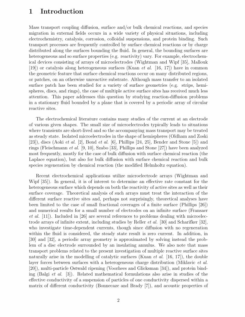
Consider a periodic array of circular disc-shaped microelectrodes distributed over anotherwise insulating boundary as illustrated in Figure 1. An electrolytic solution fillsthe entire volume above the plane, and we are interested in calculating the steady-state current to the surface due to oxidation-reduction processes that occur on thesurface of the electrodes; effects due to possible chemical regeneration in the bulk arealso considered. The flux of the given chemical to the electrode is proportional to themeasured electrode current, and so we seek a solution for the concentration flux of thechemical species. We assume that there is no fluid motion, so the usual reaction-diffusionequations apply as in the literature cited above.

The electrode surfaces are denoted SE and the insulating planar region is denotedSP . We choose coordinates such that the insulating plane is at z = 0, and the electrolyticsolution fills the volume z > 0. Following Phillips [24, 25] (see also Bender and Stone[5]), the steady state reaction-diffusion problem may be written in the dimensionlessform

∇2φ = α2φ where

φ = 1 +1

K

∂φ

∂zon z = 0, r ∈ SE ,

∂φ

∂z= 0 on z = 0, r ∈ SP ,

φ → 0 as z → ∞,

(1)

where φ(r) is the dimensionless concentration in the fluid, α2 is a constant representingthe ratio of bulk species regeneration relative to diffusion, K is a constant representingthe ratio of surface reaction rate at the electrode surface relative to diffusion in the bulk,and r denotes the position vector. A large value of α indicates a large bulk regeneration,and so most activity will take place near the electrode, while a small value of α indicatesdiffusion becoming more important, as reactants must be transported inwards frominfinity rather than being regenerated near the electrode. An infinite value for K is thelimit in which reaction takes place instantaneously at the electrode. Smaller values of

3

S - Electrodes

S - Insulating Plate

E

P

z=0x

yz

r=1

Figure 1: The periodic array of microelectrodes on an insulating plane.

K indicate a slower surface reaction at the electrode. In the limit K = 0, no surfacereaction takes place and the solution is φ = 0 everywhere (the first boundary conditionof (1) reduces to ∂φ/∂z = 0 on z = 0, r ∈ SE). Equation (1) can be recognized as themodified Helmholtz equation with mixed boundary conditions.

Here, we shall assume that the surface consists of rectangular periodic cells of size2l1×2l2, with circular microelectrodes of radius one centered within the periodic cells, asshown in Figure 2. Due to the periodicity, we shall only need to determine the solutionwithin a single cell. Rather than calculate the concentration φ directly, we are moreinterested in the flux ∂φ/∂z on the plane z = 0. Once the flux distribution has beencalculated, the total dimensionless flux to a single electrode follows from

Total Flux per electrode = −∫

SE

∂φ

∂zdS, (2)

which is proportional to the measured current through the electrode. Since we are onlyinterested in finding the flux distribution over the electrode, the domain of applicationof (1) is the infinite half-space, and, additionally, as the boundary value problem islinear, an integral equation approach is ideal. This mathematical approach is common,although some of the analytical details necessary to treat the periodic surface conditionand numerical details to represent the flux accurately require some care.

4

x

yz

SE

SP

l2

l1

Ssides

Vc

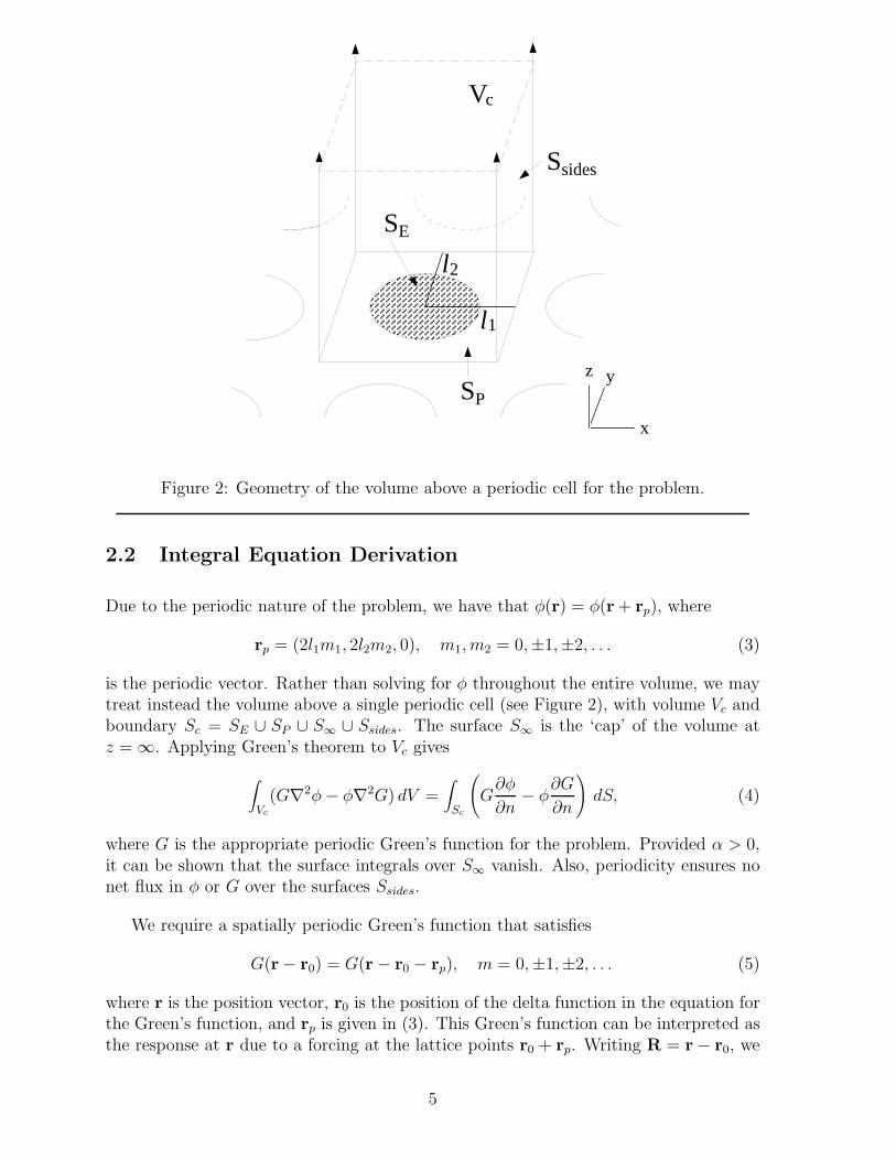
Figure 2: Geometry of the volume above a periodic cell for the problem.

2.2 Integral Equation Derivation

Due to the periodic nature of the problem, we have that φ(r) = φ(r + rp), where

rp = (2l1m1, 2l2m2, 0), m1, m2 = 0,±1,±2, . . . (3)

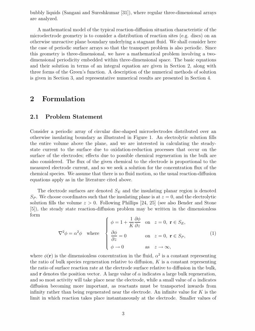
is the periodic vector. Rather than solving for φ throughout the entire volume, we maytreat instead the volume above a single periodic cell (see Figure 2), with volume Vc andboundary Sc = SE ∪ SP ∪ S∞ ∪ Ssides. The surface S∞ is the ‘cap’ of the volume atz = ∞. Applying Green’s theorem to Vc gives

∫

Vc

(G∇2φ − φ∇2G) dV =∫

Sc

(

G∂φ

∂n− φ

∂G

∂n

)

dS, (4)

where G is the appropriate periodic Green’s function for the problem. Provided α > 0,it can be shown that the surface integrals over S∞ vanish. Also, periodicity ensures nonet flux in φ or G over the surfaces Ssides.

We require a spatially periodic Green’s function that satisfies

G(r− r0) = G(r − r0 − rp), m = 0,±1,±2, . . . (5)

where r is the position vector, r0 is the position of the delta function in the equation forthe Green’s function, and rp is given in (3). This Green’s function can be interpreted asthe response at r due to a forcing at the lattice points r0 + rp. Writing R = r − r0, we

5

have that the Green’s function must satisfy

∇2rG(R) = α2G(R) +

∞∑

m1=−∞

∞∑

m2=−∞δ(R − rp) with G → 0 as |R3| → ∞, (6)

where the Laplacian operator is with respect to the variable r, and R3 is the z-componentof R.

Given an appropriate solution of (6), which is described in detail in section 2.3, theGreen’s function is substituted into (4), and the source point r0 moved to the boundary(as is standard in applications of the boundary integral method, e.g. Brebbia et al. [8]).Thus, we arrive at

−1

2φ(r0) =

∫

SE∪SP

(

G(R)∂φ

∂n(r) − φ(r)

∂G

∂n(R)

)

dS(r), r0 ∈ SE ∪ SP . (7)

Since the surface SE ∪ SP is that part of the periodic cell boundary in the plane z = 0,we have that ∂/∂n ≡ −∂/∂z, and it may be shown that ∂G/∂z = 0 when both r andr0 are on the plane z = 0 (R3 = 0). Thus, (7) reduces to

1

2φ(r0) =

∫

SE∪SP

G(R)∂φ

∂z(r) dS(r). (8)

Finally, applying the boundary conditions on SE and SP from (1), we obtain the integralformulation for the flux of φ through the electrode as

1 +1

Kφ′(r0) =

∫

SE

2G(r− r0)φ′(r) dS(r), r0 ∈ SE, (9)

where we have written φ′ for ∂φ/∂z. We note that r0 need only be taken over the surfaceof the electrode SE , where SE is the disc of radius one centered at the origin on the planez = 0. The specific geometry of the periodic surface (the parameters l1 and l2) enter theproblem through the Green’s function G as described in the next section.

2.3 The Periodic Green’s Function

To find the Green’s function, we first note that r0 is fixed as the position r is varied, so∇2

r≡ ∇2

R, and (6) can be written as

∇2RG(R) = α2G(R) + δ(R3)

∑

m

δ(R1 − 2l1m1)δ(R2 − 2m2l2), (10)

where we have used the definition of rp and written∑

m to represent the infinite doublesummation over m1 and m2. To solve (10), we make use of two-dimensional Fouriertransforms F2 in (R1, R2), as defined in Nijboer and De Wette [22]:

F2f(R1, R2) = f(k1, k2) =∫ ∞

−∞

∫ ∞

−∞e2πi(k1R1+k2R2)f(R1, R2) dR2 dR1,

F−12

{

f(k1, k2)}

= f(R1, R2) =∫ ∞

−∞

∫ ∞

−∞e−2πi(k1R1+k2R2)f(k1, k2) dk2 dk1.

(11)

6

Taking the two-dimensional Fourier transform of (10), and using the standard result(Barton [4]) that

∑

m

δ(x1 − m1L1)δ(x2 − m2L2) =1

L1L2

∑

m

e2πi

(

m1x1

L1+

m2x2

L2

)

, (12)

we obtain the equation

∂2G

∂R23

−(

4π2(k21 + k2

2) + α2)

G =δ(R3)

4l1l2

∑

m

δ(

k1 −m1

2l1

)

δ(

k2 −m2

2l2

)

, (13)

which has the solution

G = − e−|R3|√

4π2(k2

1+k2

2)+α2

8l1l2√

4π2(k21 + k2

2) + α2

∑

m

δ(

k1 −m1

2l1

)

δ(

k2 −m2

2l2

)

. (14)

Using the inverse transform, we obtain the Green’s function

G(R) = −∑

m

exp

{

−πi(

m1R1

l1+ m2R2

l2

)

− |R3|√

π2

[

(

m1

l1

)2+(

m2

l2

)2]

+ α2

}

8l1l2

√

π2

[

(

m1

l1

)2+(

m2

l2

)2]

+ α2

. (15)

Note that in (9), both r and r0 lie on the plane z = 0, so that R3 = 0, which is a usefulsimplification for some of the mathematical manipulations that follow.

2.4 Accelerating the Convergence Rate of the Green’s Function

The form of the Green’s function given in (15) is computationally inefficient becausethe convergence rate is very slow when |R3| is small or zero, and a large number ofterms are required to calculate (15) to even a few figures of accuracy. A more usefulform of the Green’s function can be obtained using various acceleration techniques suchas the Poisson summation formula or the method of Ewald. We mention at this pointthat the double summation over m1 and m2 is calculated by starting with the termm1 = m2 = 0 and adding successive layers corresponding to |m1|+ |m2| = j, j = 1, 2, . . .. Geometrically, this ensures that the partial sum is that of a square of terms surroundingm1 = m2 = 0.

2.4.1 The Poisson Summation Formula

The principle of the Poisson summation formula is that the Fourier transform of asmooth function approaches zero more rapidly than the original function. The Poissonsummation formula in one dimension is clearly outlined in Barton [4], and the two-dimensional form can constructed using the same procedure:

∑

m

F (λ1m1, λ2m2) =1

λ1λ2

∑

m

∫ ∞

−∞

∫ ∞

−∞F (ξ1, ξ2)e

2πi

(

m1ξ1λ1

+m2ξ2

λ2

)

dξ2dξ1. (16)

7

Applying (16) to (15), we find

G(R) = −1

8

∑

m

∫ ∞

−∞

∫ ∞

−∞

e−πi(ξ1k1+ξ2k2)−|R3|√

π2(ξ2

1+ξ2

2)+α2

√

π2(ξ21 + ξ2

2) + α2dξ2dξ1, (17)

where (k1, k2) = (R1−2l1m1, R2−2l2m2). Transforming to polar coordinates using ξ1 =a cos θ, ξ2 = a sin θ, and k1 = k cos ϕ, k2 = k sin ϕ with k2 = (R1−2l1m1)

2+(R2−2l2m2)2,

and using equation (3.915.2) from Gradshteyn and Ryzhik [12],∫ π

0eiβ cos x cos(nx) dx = inπJn(β), (18)

we obtain

G(R) = −π

4

∑

m

∫ ∞

0

aJ0(πka)√π2a2 + α2

e−|R3|√

π2a2+α2

da. (19)

Applying the transform a2 = α2(u2 − 1)/π2, and using equation (6.616.2) from Grad-shteyn and Ryzhik [12] that

∫ ∞

1e−αxJ0

(

β√

x2 − 1)

dx =1√

α2 + β2e−

√α2+β2

, (20)

equation (19) becomes

G(R) = − 1

4π

∑

m

exp[

−α√

R23 + k2

]

√

k2 + R23

,

= − 1

4π

∑

m

exp[

−α√

(R1 − 2m1l1)2 + (R2 − 2m2l2)2 + R23

]

√

(R1 − 2m1l1)2 + (R2 − 2m2l2)2 + R23

.

(21)

From this exponential form of G(R), it can be shown that ∂G/∂z = 0 when R3 = 0, aswas required in the derivation of (9).

The representation of the Green’s function in (21) is the same as would be ob-tained by distributing the three-dimensional free-space Green’s function for the modifiedHelmholtz equation

G(r − r0) = − 1

4π

e−α|r−r0|

|r− r0|(22)

over all the electrodes to deal with spatial periodicity. Of course, (22) could have beenwritten down immediately, but it is useful to understand the steps (16-21) in order toapply the Ewald method to this problem.

While the exponential in the summation for G(R) in (21) ensures that its convergenceis faster than for (15), the convergence rate can still be quite poor for small α. In suchcases, we will use the method of Ewald, which we now outline.

2.4.2 The Method of Ewald

The method of Ewald is a technique for improving the convergence rates of slowlyconverging lattice sums. We assume R3 = 0 in the derivation that follows.

8

We wish to accelerate the convergence of

G(R) = −∑

m

exp[

−πi(

m1R1

l1+ m2R2

l2

)]

8l1l2

√

π2

{

(

m1

l1

)2+(

m2

l2

)2}

+ α2

. (23)

Using the fact that erf(x) + erfc(x) = 1, we rewrite (23) as

G(R) = S1 + S2, (24)

where

S1 = −∑

m

exp[

−πi(

m1R1

l1+ m2R2

l2

)]

erfc(

c√

A)

8l1l2√

A,

S2 = −∑

m

exp[

−πi(

m1R1

l1+ m2R2

l2

)]

erf(

c√

A)

8l1l2√

A,

(25)

A = π2{(m1/l1)2 + (m2/l2)

2} + α2, and c is an arbitrary constant. Due to the natureof the complimentary error function, the sum S1 converges very quickly, but the rateof convergence of S2 is unchanged. The Ewald method as described in Nijboer and DeWette [22] accelerates the convergence of S2 by first converting the summation terms intointegrals using properties of the delta function, and then applying the Fourier convolutiontheorem to accelerate convergence. However, the same final result can be obtained moreeasily by applying the two-dimensional Poisson’s summation formula to S2. Identifyingλi = 1/li, and applying (16) to (25b), we find that

S2 = −∑

m

1

4

∫ ∞

−∞

∫ ∞

−∞e−πi(k1ξ1+k2ξ2)

erf(

c√

π2(ξ21 + ξ2

2) + α2)

√

π2(ξ21 + ξ2

2) + α2dξ2dξ1, (26)

where (k1, k2) = (R1 − 2m1l1, R2 − 2m2l2). Since d(erf(x))/dx = 2 exp(−x2)/√

π, wemay take the derivative of S2 with respect to c to show that

dS2

dc= −

∑

m

1

2c2π3/2e−α2c2− k2

4c2 , (27)

where k2 = k21 + k2

2, and we have (Gradshteyn and Ryzhik [12], equation (3.896.4))

∫ ∞

0e−βx2

cos(bx)dx =1

2

√

π

βe−

b2

4β , Re(β) > 0. (28)

Now, integrating (27) leads to

S2 = −∑

m

1

4πk

[

ekαerfc

(

k

2c+ αc

)

+ e−kαerfc

(

k

2c− αc

)]

, (29)

where we have used (Abramowitz and Stegun [1], equation (7.4.33))

∫

e−a2x2− b2

x2 dx =

√π

4a

[

e2aberf

(

ax +b

x

)

+ e−2aberf

(

ax − b

x

)]

+ C. (30)

9

Thus, we have the final result that when R3 = 0,

G(R) = − 1

4l1l2

∑

m

eπi

(

m1R1

l1+

m2R2

l2

)

erfc(c√

A)√A

− 1

4π

∑

m

1

k

[

ekαerfc

(

k

2c+ αc

)

+ e−kαerfc

(

k

2c− αc

)]

,

(31)

where

k =√

(R1 − 2l1m1)2 + (R2 − 2l2m2)2 and A = π2

{

(

m1

l1

)2

+(

m2

l2

)2}

+ α2. (32)

The arbitrary parameter c is chosen to obtain the best convergence for G(R). Since

erfc(x) = O(

e−x2)

for x ≫ 1, we can balance the convergence rates of the complimentary

error function terms in (31) to arrive at the estimate

c =

√

l1l2π

. (33)

2.4.3 Choosing an Acceleration Technique

The convergence rate of G(R) depends on α, and the geometric parameters l1 and l2.While the convergence rate for G(R) using the Ewald sum (31) has been found to berelatively insensitive to the value of α, and the convergence rate of the Ewald sum isO(

e−m2)

compared to the O (e−m) rate of the Poisson sum (21), it is not an automaticchoice to always use the Ewald result rather than the Poisson sum. Each term of theEwald sum requires the calculation of three complimentary error functions, while thePoisson sum terms only require evaluation of a single exponential function. Thus froma computational view, the Poisson sum may be more efficient than the Ewald sum.

Our initial choice for calculating the complimentary error function was the routinederfc() from the IMSL numerical package [36]. However, this routine was found tobe significantly slower than polynomial approximations for erfc tabulated in Hart [13].The particular polynomial approximations chosen from [13] for erfc are tables 5665on [0, 2.5), 5705 on [2.5, 5.5) and thirteen terms in the asymptotic expansion of thecomplimentary error function (from Abramowitz and Stegun [1]) on [5.5,∞). Thesepolynomial approximations guarantee at least eleven digits of accuracy and an absoluteerror of less than 10−15, and are approximately seven times faster than the IMSL routineon a Sun Sparc 10.

To decide which of the Ewald and Poisson sum results to use for calculating G(R),a computational comparison is made. The sums are calculated in layers as describedin section 2.4 above until a relative error of 10−8 is obtained. The Green’s function iscalculated for 105 cases at the points R = (r cos θ, r sin θ), where r = 0, 0.2, 0.4, . . . , 2,and θ = 0, π/50, π/25, . . . , 2π, which spans the values of R at which the Green’s functionneeds to be calculated. The total time (in CPU seconds) needed to calculate the Green’sfunction using the Ewald and Poisson sum results are compared, and for a particular

10

0 5 10 15 20 25 300.0

0.5

1.0

1.5

2.0

α 0

Use Ewald sum

Use Poisson sum

l2

l1=l2

l1=1.05

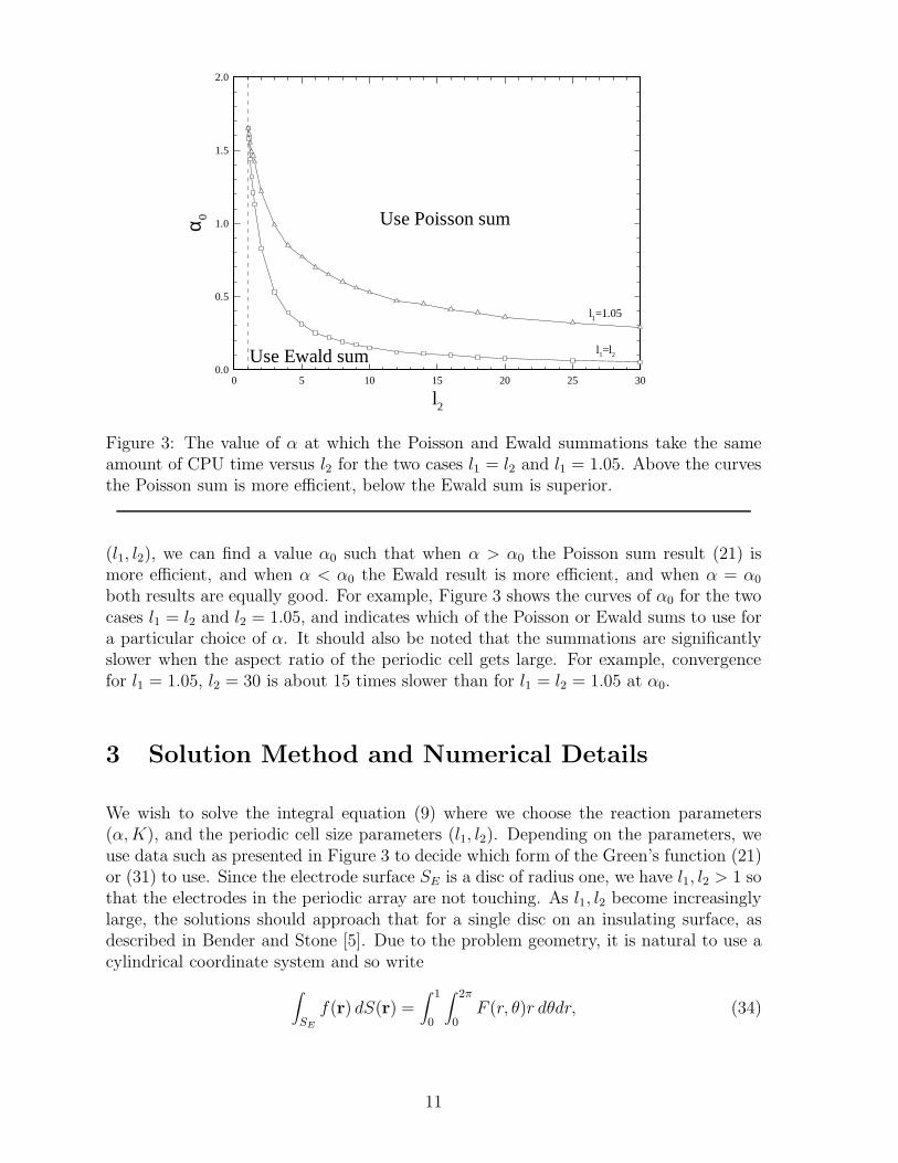
Figure 3: The value of α at which the Poisson and Ewald summations take the sameamount of CPU time versus l2 for the two cases l1 = l2 and l1 = 1.05. Above the curvesthe Poisson sum is more efficient, below the Ewald sum is superior.

(l1, l2), we can find a value α0 such that when α > α0 the Poisson sum result (21) ismore efficient, and when α < α0 the Ewald result is more efficient, and when α = α0

both results are equally good. For example, Figure 3 shows the curves of α0 for the twocases l1 = l2 and l2 = 1.05, and indicates which of the Poisson or Ewald sums to use fora particular choice of α. It should also be noted that the summations are significantlyslower when the aspect ratio of the periodic cell gets large. For example, convergencefor l1 = 1.05, l2 = 30 is about 15 times slower than for l1 = l2 = 1.05 at α0.

3 Solution Method and Numerical Details

We wish to solve the integral equation (9) where we choose the reaction parameters(α, K), and the periodic cell size parameters (l1, l2). Depending on the parameters, weuse data such as presented in Figure 3 to decide which form of the Green’s function (21)or (31) to use. Since the electrode surface SE is a disc of radius one, we have l1, l2 > 1 sothat the electrodes in the periodic array are not touching. As l1, l2 become increasinglylarge, the solutions should approach that for a single disc on an insulating surface, asdescribed in Bender and Stone [5]. Due to the problem geometry, it is natural to use acylindrical coordinate system and so write

∫

SE

f(r) dS(r) =∫ 1

0

∫ 2π

0F (r, θ)r dθdr, (34)

11

where F (r, θ) ≡ f(r cos θ, r sin θ). Due to the symmetry of the problem, we only needto find φ′ in the first quadrant, and (9) can then be rewritten as

1 +1

Kφ′(r0, θ0) =

∫ 1

0

∫ π/2

02φ′(r, θ)r{G(r, θ; r0, θ0) + G(r, π − θ; r0, θ0)+

G(r, π + θ; r0, θ0) + G(r, 2π − θ; r0, θ0)} dθdr,

for 0 ≤ θ0 < π/2, 0 ≤ r0 < 1,

(35)

where G(r, θ; r0, θ0) ≡ G(R) = G(r − r0) and we have explicitly written the unknownflux φ′ in polar coordinates.

To find the unknown flux φ′, we divide the rectangle [0, 1] × [0, π/2] in polar coor-dinates into M × N elements, and assume that φ′ varies quadratically in r and θ; onthe (i, j)th element, we assume φ′ =

∑

k φ′ijkNk(η1, η2), where (η1, η2) is the coordinate

system for the (i, j)th element mapped onto [−1, 1]×[−1, 1], Nk are the quadratic weightfunctions, and the φ′

ijk are unknowns. By choosing the collocation points (r0, θ0) to bethe node points of the quadratic elements, we convert (35) to a linear system of equationsfor the φ′

ijk, which can be solved by Gaussian elimination to obtain a solution for theflux. Further details on the quadratic element boundary element method can be foundin standard boundary element texts such has Brebbia et al. [8].

3.1 Integration Techniques

The matrix elements in the linear system to be inverted involve two-dimensional inte-grals over the elements of the Green’s function multiplied by the appropriate weightfunctions. If the current collocation point (r0, θ0) is on the border or within the regionwe are integrating over, then there is a singularity in the function at that point, whichmust be handled more carefully. Here, we implement a scheme using ‘degenerate quadri-laterals’, originally described in Lachat and Watson [18]. If we transform a triangle ontoa square, and stretch a corner of the triangle onto one of the square’s sides, then theJacobian of the transformation is such that a 1/r singularity at the stretched corner ofthe triangle is removed, and no longer causes poor convergence for numerical integra-tion rules. This idea is analogous to transforming a local cartesian coordinate systemto polar coordinates with the origin at the singularity, and has the advantage that thedegenerate quadrilateral transformation does not have to deal with circular arcs. Anintegration routine designed to integrate over a set of general quadrilaterals, given theirfour corners, thus has the advantage of being able to integrate over rectangular regionswith no singularities (given the four corners) or deal with singularities in the region(divide into a set of triangles, with the singularity at a corner). Furthermore, the abilityto integrate over a set of quadrilaterals is also useful in cases where elements have a highaspect ratio. For example, for long, thin integration regions, more function evaluationsare usually required in the long direction to obtain suitable accuracy. It follows that,for the same accuracy, far fewer function evaluations are required if initially long thinregions are subdivided into smaller regions of lower aspect ratio. Numerical experimentsperformed here indicate that setting the maximum aspect ratio of a rectangle equal to2 gives the best efficiency.

12

Another integration difficulty which arises in boundary integral calculations lies inchoosing the order of the quadrature rule. Integrals over regions near the collocationpoint will typically require more effort than those far from it, but a simple distance ruleis often insufficient, since the shape of the integration region is also important. Here, weuse a combination of successive and adaptive quadrature rules in an attempt to producea single integration routine to deal with the range of integrals required in a boundaryelement method. An initial approximation is made using 4 × 4 and 6 × 6 point Gauss-Legendre rules over general quadrilaterals, with an error estimate based on the differencebetween these rules. For a more detailed description of the error estimate, see Kahanerand Rechard [15]. If the error estimate is larger than that required, continue with 8× 8and 12 × 12 point rules. If the required accuracy has still not been obtained, use anadaptive method, where the quadrilateral with the largest error is subdivided into fournew quadrilaterals, and the 8 × 8 and 12 × 12 point rules are applied to them. Thisadaptive process is continued until the estimated error is less than that requested. Thiscombination of successive then adaptive algorithms has the advantage that it will notuse a high order rule when not necessary (i.e. when the integration region is far from thecollocation point), but will use efficient adaptive methods with reasonably high-orderrules when required.

Finally, we note that evaluating the periodic Green’s function (21) or (31) is sub-stantially more expensive than evaluating the free space Green’s function (22). Since fora quadratic boundary element method we integrate over each region for each collocationpoint eight times where the Green’s function is multiplied by different weight functions,it makes sense to form all eight integrals one time, and use vector integration. In casessuch as this where each of the integrands in the vector are very similar (different weightfunctions), substantial savings in time can be made by minimizing the number of timesthe Green’s function has to be evaluated. For this problem a factor of 5 increase in speedof integration was obtained by changing from scalar to vector integration.

For the work described here, numerical integration is performed with a requestedrelative error of 5 × 10−6, which guarantees at least 5 digits of accuracy.

3.2 Singularities in the Solution

Unfortunately, when the above procedures are used to solve the integral equation (35),the numerical solutions converge quite slowly as the number of quadratic elements isincreased. The numerical inaccuracies arise because the function we are trying to find, φ′,is itself poorly behaved as we approach the edge of the disc. The problem is qualitativelydifferent in the two cases K = ∞ and 0 < K < ∞, which are now addressed separately.

3.2.1 The K = ∞ Case

In this case, the boundary conditions from (1) on z = 0 become φ = 1 for r ∈ SE and∂φ/∂z = 0 for r ∈ SP . For the case of a single disc, not the periodic array, there is anexact analytic solution for the case α = 0, the so-called ‘electrified disc’ solution (seefor example Jackson [14] or Newman [21]), where the flux on the surface of the disc in

13

terms of radial position r is∂φ

∂z= − 2

π√

1 − r2. (36)

The flux distribution has an inverse square root singularity at the edge of the disc, r = 1,which explains why a quadratic element approximation is relatively poor. This inversesquare root singularity is common in problems where there is a change in boundaryconditions, as is also the case in the stress field at a crack tip in classical elastostatics.

For the modified Helmholtz equation, analytic information on the leading term inthe solution near the singularity can be found following the method described in Ra-machandran [29] for Laplace’s equation near the point where the boundary conditionssuddenly change. We find that the leading order behavior near the edge x = 1− r of φ′

is φ′ ∝ I1/2(αx)xr, where I is the modified Bessel function of the first kind. For smallx (near the singularity), φ′ ∝ 1/

√x, and so the form of the singularity is the same as

for Laplace’s equation, which is the modified Helmholtz equation with α = 0. In fact,the solution has this inverse square root singularity in the flux φ′ regardless of the valueof α or whether we are dealing with a single or periodic array of electrodes. Thus, wereplace φ′(r, θ) in the integral equation (35) by φ′(r, θ)/

√1 − r, and solve for φ′. The

inverse square root singular part of the flux is absorbed into the formulation, and thesmooth contribution to the flux is all that remains to be approximated by the quadraticelements.

The additional 1/√

1 − r term in the integral means that there is an additionalsingularity in the two-dimensional integrals over the elements whose edge correspondsto the edge of the disc. Transformations to remove endpoint algebraic singularities areavailable in Press et al. [28], and we make use of the identity

∫ 1

−1

f(x)√1 − x

dx =∫ 1

−1

√2f(

1 − 1

2(1 − t)2

)

dt (37)

to remove the square root singularity at r = 1.

The 1/√

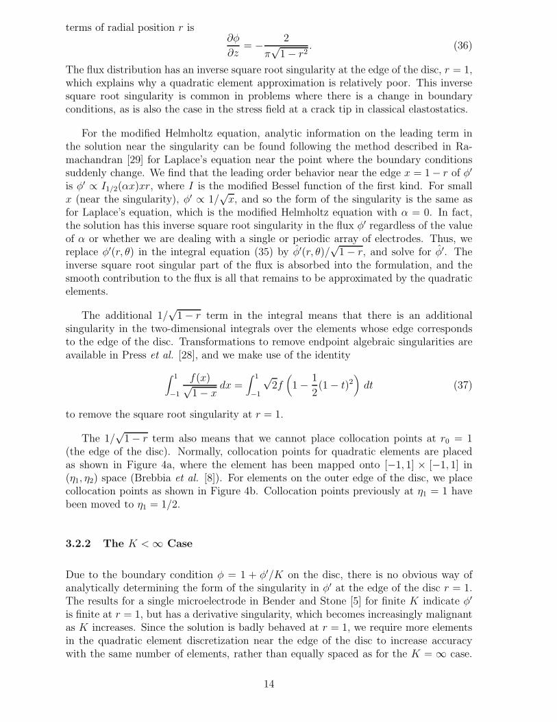
1 − r term also means that we cannot place collocation points at r0 = 1(the edge of the disc). Normally, collocation points for quadratic elements are placedas shown in Figure 4a, where the element has been mapped onto [−1, 1] × [−1, 1] in(η1, η2) space (Brebbia et al. [8]). For elements on the outer edge of the disc, we placecollocation points as shown in Figure 4b. Collocation points previously at η1 = 1 havebeen moved to η1 = 1/2.

3.2.2 The K < ∞ Case

Due to the boundary condition φ = 1 + φ′/K on the disc, there is no obvious way ofanalytically determining the form of the singularity in φ′ at the edge of the disc r = 1.The results for a single microelectrode in Bender and Stone [5] for finite K indicate φ′

is finite at r = 1, but has a derivative singularity, which becomes increasingly malignantas K increases. Since the solution is badly behaved at r = 1, we require more elementsin the quadratic element discretization near the edge of the disc to increase accuracywith the same number of elements, rather than equally spaced as for the K = ∞ case.

14

-1 0 1

-1

0

1

η2

η1

-1 0 1

-1

0

1

η2

η1

1/2

(a) (b)

Figure 4: Positions of collocation points for a quadratic element transformed to (η1, η2)space, (a) normally and (b) when the element is on the edge of the disc, with the nodespositioned to avoid the inverse square root singularity at r = 1.

To this end, we place M/2 elements in the r direction on r ∈ [0, 0.9] and M/2 elementson r ∈ [0.9, 1].

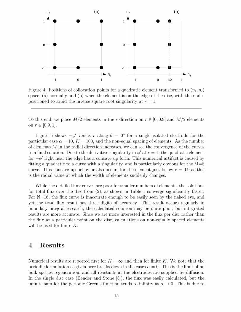
Figure 5 shows −φ′ versus r along θ = 0◦ for a single isolated electrode for theparticular case α = 10, K = 100, and the non-equal spacing of elements. As the numberof elements M in the radial direction increases, we can see the convergence of the curvesto a final solution. Due to the derivative singularity in φ′ at r = 1, the quadratic elementfor −φ′ right near the edge has a concave up form. This numerical artifact is caused byfitting a quadratic to a curve with a singularity, and is particularly obvious for the M=8curve. This concave up behavior also occurs for the element just below r = 0.9 as thisis the radial value at which the width of elements suddenly changes.

While the detailed flux curves are poor for smaller numbers of elements, the solutionsfor total flux over the disc from (2), as shown in Table 1 converge significantly faster.For N=16, the flux curve is inaccurate enough to be easily seen by the naked eye, andyet the total flux result has three digits of accuracy. This result occurs regularly inboundary integral research; the calculated solution may be quite poor, but integratedresults are more accurate. Since we are more interested in the flux per disc rather thanthe flux at a particular point on the disc, calculations on non-equally spaced elementswill be used for finite K.

4 Results

Numerical results are reported first for K = ∞ and then for finite K. We note that theperiodic formulation as given here breaks down in the cases α = 0. This is the limit of nobulk species regeneration, and all reactants at the electrodes are supplied by diffusion.In the single disc case (Bender and Stone [5]), the flux was easily calculated, but theinfinite sum for the periodic Green’s function tends to infinity as α → 0. This is due to

15

0.0 0.1 0.2 0.3 0.4 0.5 0.6 0.7 0.8 0.99.0

9.1

9.2

9.3

9.4

9.5

9.6

9.7

9.8

9.9

10.0

r

M=8M=16

M=32,64

-φ′

0.90 0.92 0.94 0.96 0.98 1.0010

15

20

25

30

M=8

M=16

M=32

M=64

Figure 5: -φ′ versus r for θ = 0◦ for a single microelectrode, varying the number ofelements. The parameters are α = 10, K = 100, and curves are for various numbersof elements in the r direction. The larger graph shows −φ′ on r ∈ [0, 0.9], with theinset showing the results on r ∈ [0.9, 1]. M represents the number of elements in the rdirection for the different solutions.

M Total flux2 31.5480714 31.0425028 30.94283916 30.91937532 30.91403364 30.912789

Table 1: Convergence of the total flux for a single disc with α = 10 and K = 100 asthe number of unknowns is increased. M is the number of quadratic elements in ther-direction.

16

the denominator of (15) tending to zero as α tends to zero for the term m1 = m2 = 0.In fact, as α → 0, the flux through each electrode in the periodic array goes to zero. Inthe single electrode case, diffusion can bring reactants to the electrode from the entirespace z > 0, and it is possible to have a nonzero flux on the disc as φ and φ′ go to zero atinfinity. For the periodic array, each electrode can only absorb reactants diffused fromthe volume above its own periodic cell in the α = 0 case, and since φ′ = 0 at z = ∞, the‘top’ of the periodic volume, conservation implies that there is no flow of reactants, andthe flux goes to zero. Thus, while no results can be calculated for the periodic problemwith α = 0, there can be assumed to be a zero flux, regardless of K, as long as l1 andl2, the periodic cell size parameters, are finite. While there are a set of problems wherethere is a nonzero concentration gradient at infinity, the current formulation cannot dealwith such a case, and is beyond the scope of this paper.

It should also be noted that by changing the Green’s function to the free-space form(22), the quadratic boundary element method described above can be used to reproducethe results of Bender and Stone [5] for a single disc on an insulating surface. In all cases,the different numerical implementations gave identical results to the reported accuracies.

4.1 Results for K = ∞

We present first the results for the case of instantaneous reaction at the electrode surface,the limit K = ∞. The assumption of an inverse square root singularity in the solutiondescribed in section 3.2.1 above was successful for all these cases. We found that 5×5 =25 elements are sufficient to give flux results which are almost indistinguishable fromhigher order discretizations, and the results for total flux through an electrode, calculatedusing (2), are accurate to at least 3 digits. The accuracy is highest for small α, up to6 digits, and diminishes as α increases, owing to the formation of boundary layers withlarge gradients. 5 × 5 quadratic elements produce a linear system of equations with 96unknowns, for which the solution with l1 = l2 takes 10 minutes of CPU time on a SunSparc 10 workstation. For periodic cells with l1 6= l2, the computation times can bemuch longer – up to 150 minutes for l1 = 1.05 and l2 = 30, for example.

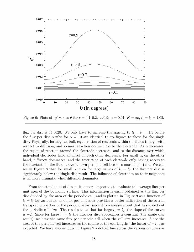
We first show the θ-dependence of the flux φ′. Figure 6 plots −φ′ as a function of r,θ for the parameters α = 0.01, K = ∞ and l1 = l2 = 1.05 in the first quadrant. On thediagonal θ = 45◦, the flux takes its maximum value. This response is expected, sincethe distance to the nearest disc is highest at this angle.

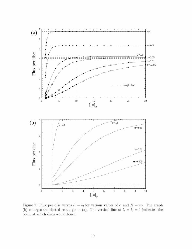
Figure 7 shows the total flux per disc as a function of l1 = l2 for various values ofα; Figure 7(b) is a magnification of the dotted rectangle in Figure 7(a). The horizontaldashed lines in Figure 7(a) represent the results for a single disc on the insulating surface,while the vertical line in Figure 7(b) at l1 = l2 = 1 indicates where electrodes touch.Figure 8 shows this information by plotting flux per disc versus α for various valuesof l1 = l2. Not surprisingly, as l1 = l2 increase in size, the flux per disc approachesthat for a single disc. As α increases, the approach to the single disc result is muchmore rapid. Not plotted in Figure 7 are results for α = 5, where the single disc fluxis 18.9931 and for l1 = l2 = 1.05 the flux per disc is 18.1444. Even more extreme arethe results for α = 10, where the single disc flux is 34.6453 and for l1 = l2 = 1.05 the

17

0 10 20 30 40 50 60 70 80 900.010

0.011

0.012

0.013

0.014

0.015

0.016

0.017

-φ⁄

r=0.9

r=0.8

r=0.7

r=0.1

θ (in degrees)

Figure 6: Plots of -φ′ versus θ for r = 0.1, 0.2, . . . 0.9; α = 0.01, K = ∞, l1 = l2 = 1.05.

flux per disc is 34.3020. We only have to increase the spacing to l1 = l2 = 1.5 beforethe flux per disc results for α = 10 are identical to six figures to those for the singledisc. Physically, for large α, bulk regeneration of reactants within the fluids is large withrespect to diffusion, and so most reaction occurs close to the electrode. As α increases,the region of reaction around the electrode decreases, and so the distance over whichindividual electrodes have an effect on each other decreases. For small α, on the otherhand, diffusion dominates, and the restriction of each electrode only having access tothe reactants in the fluid above its own periodic cell becomes more important. We cansee in Figure 8 that for small α, even for large values of l1 = l2, the flux per disc issignificantly below the single disc result. The influence of electrodes on their neighborsis far more dramatic when diffusion dominates.

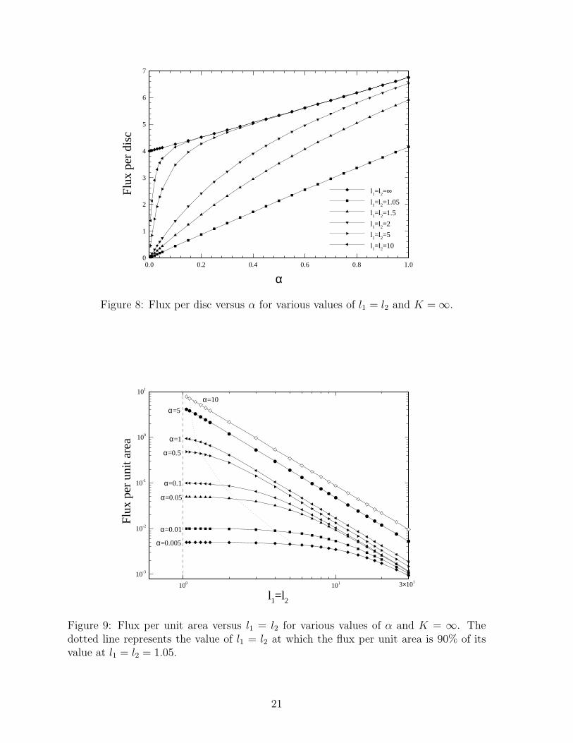
From the standpoint of design it is more important to evaluate the average flux perunit area of the bounding surface. This information is easily obtained as the flux perdisc divided by the area of the periodic cell, and is plotted in Figure 9 as a function ofl1 = l2 for various α. The flux per unit area provides a better indication of the overalltransport properties of the periodic array, since it is a measurement that has scaled outthe periodic cell size. The results show that for large l1 = l2, the slope of the curvesis −2. Since for large l1 = l2 the flux per disc approaches a constant (the single discresult), we have the same flux per periodic cell when the cell size increases. Since thearea of the periodic cell increases as the square of the cell lengths, the factor of −2 is asexpected. We have also included in Figure 9 a dotted line across the various α curves as

18

0 1 2 3 4 5 6 7 8 9 10

0

1

2

3

4

Flu

x pe

r di

sc

α=0.005

α=0.01

α=0.05

α=0.1α=0.5

l1=l2

(b)

0 5 10 15 20 25 300

1

2

3

4

5

6

7

Flu

x pe

r di

sc

single disc

α=1

α=0.5

α=0.1α=0.05

α=0.01α=0.005

l1=l2

(a)

Figure 7: Flux per disc versus l1 = l2 for various values of α and K = ∞. The graph(b) enlarges the dotted rectangle in (a). The vertical line at l1 = l2 = 1 indicates thepoint at which discs would touch.

19

a measure of the effectiveness of close-packing the electrodes on the insulating surface.The dotted line is the value of l1 = l2 at which the flux per unit area is 90% of its valueat l1 = l2 = 1.05, and we can see that as α decreases, this value increases. It is thusevident that placing electrodes closer together yields a much smaller additional increasein flux for small α. Since placing electrodes closer together is presumably more expensivein terms of time and materials, a point may be reached where placing electrodes closertogether is uneconomical. This argument is even more important if the catalytic analogof this problem is considered, in which case the flux relates to the total reaction in thesystem due to catalytic sites, which we may be trying to maximize.

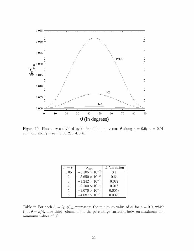
We also include here comparisons of the variation of φ′ with respect to angle θ as thesize of the periodic cell increases. Figure 10 shows curves of flux divided by its minimumvalue for α = 0.01, r = 0.9, θ in the first quadrant, and varying the periodic cell size.The curves have been scaled by the values of the flux at r = 0.9 and θ = 0◦, so that thevariations are emphasised. Table 2 reports the values of the flux at r = 0.9 and θ = 45◦

for the various periodic cell sizes, and shows the percentage variation between maximumand minimum φ′ values. We see that the percentage variation is decreasing more rapidlywith increasing periodic cell size than the convergence of the φ′

min values. In fact, theflux per disc results from Figure 7 show that, for α = 0.01, the flux per disc is still wellbelow the single disc flux for l1 = l2 = 30, which indicates that the variation of φ′ with θis only due to the close proximity of the electrodes for small l1, l2. For moderate to largespacings, the discs are far enough away from each other to cause minimal disturbancesin their neighbor’s flux, but the limitations on volume available for diffusion (only thevolume above the periodic cell for each electrode) result in the low flux per disc. In fact,this observation explains the observable point of inflexion in the curves of flux per discfor α = 0.1, 0.05, 0.01, 0.05 shown earlier in Figure 7(a). There is a drop in flux per discas l1 = l2 decreases due to the reduced size of the periodic cell. However, as l1 = l2 getssmall enough, there is additional interaction between the discs themselves, causing theangular variation of φ′ observed in Figure 10.

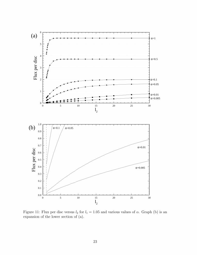
Finally, in Figure 11, the flux per disc is shown with curves for different α, but nowl1 = 1.05 always, and l2 is varied, thus increasing the aspect ratio of the periodic cell.For large l2, this geometry will look like widely separated parallel rows of discs. We seethat the convergence to a set flux per disc as l2 increases is about the same as for thel1 = l2 case. However, the value the flux per disc converges to is reduced, by a greaterfraction as α gets smaller. We also see that the inflexion in the curves in Figure 7(a)are not seen in Figure 11. Since l1 = 1.05, discs will always be close together in the xdirection, and so the change in behavior as discs get further apart is not apparent here.

4.2 Results for Finite K

For finite K, tests were performed for the single microelectrode case for various α andK with nonequally spaced elements in the radial direction. It was found that 3-6 digitsof accuracy in the total flux are obtained using M=16 elements (8 on r ∈ [0, 0.9], 8 onr ∈ [0.9, 1]), with the accuracy highest for small K. Thus, results quoted here used16 × 5 = 80 element discretizations. 16 × 5 quadratic elements lead to 283 unknowns,and solution took roughly three hours on a Sun Sparc 10. It should also be noted that

20

0.0 0.2 0.4 0.6 0.8 1.00

1

2

3

4

5

6

7

α

Flu

x pe

r di

sc

l1=l2=∞l1=l2=1.05

l1=l2=1.5

l1=l2=2

l1=l2=5

l1=l2=10

Figure 8: Flux per disc versus α for various values of l1 = l2 and K = ∞.

100 101

10-3

10-2

10-1

100

101

Flu

x pe

r un

it ar

ea

l1=l2

α=10

α=5

α=1

α=0.5

α=0.1

α=0.05

α=0.01

α=0.005

3×101

Figure 9: Flux per unit area versus l1 = l2 for various values of α and K = ∞. Thedotted line represents the value of l1 = l2 at which the flux per unit area is 90% of itsvalue at l1 = l2 = 1.05.

21

0 10 20 30 40 50 60 70 80 90

1.000

1.005

1.010

1.015

1.020

1.025

1.030

1.035

θ (in degrees)

l=1.5

l=2

l=3

φ⁄ /φ⁄ m

in

Figure 10: Flux curves divided by their minimums versus θ along r = 0.9; α = 0.01,K = ∞, and l1 = l2 = 1.05, 2, 3, 4, 5, 6.

l1 = l2 φ′min % Variation

1.05 −3.105 × 10−2 3.12 −5.650 × 10−2 0.643 −1.242 × 10−1 0.0774 −2.100 × 10−1 0.0185 −3.070 × 10−1 0.00586 −4.087 × 10−1 0.0023

Table 2: For each l1 = l2, φ′min represents the minimum value of φ′ for r = 0.9, which

is at θ = π/4. The third column holds the percentage variation between maximum andminimum values of φ′.

22

0 5 10 15 20 25 300

1

2

3

4

5

6F

lux

per

disc

l2

α=0.005α=0.01

α=0.05

α=0.1

α=0.5

α=1(a)

0 5 10 15 20 25 300.0

0.1

0.2

0.3

0.4

0.5

0.6

0.7

0.8

0.9

1.0

l2

(b)

Flu

x pe

r di

sc

α=0.005

α=0.01

α=0.05α=0.1

Figure 11: Flux per disc versus l2 for l1 = 1.05 and various values of α. Graph (b) is anexpansion of the lower section of (a).

23

the integral terms from (35) are independent of K, and so calculations for a particularα, l1, and l2 can be used for various K with minimal extra calculation - just the inversionof a matrix.

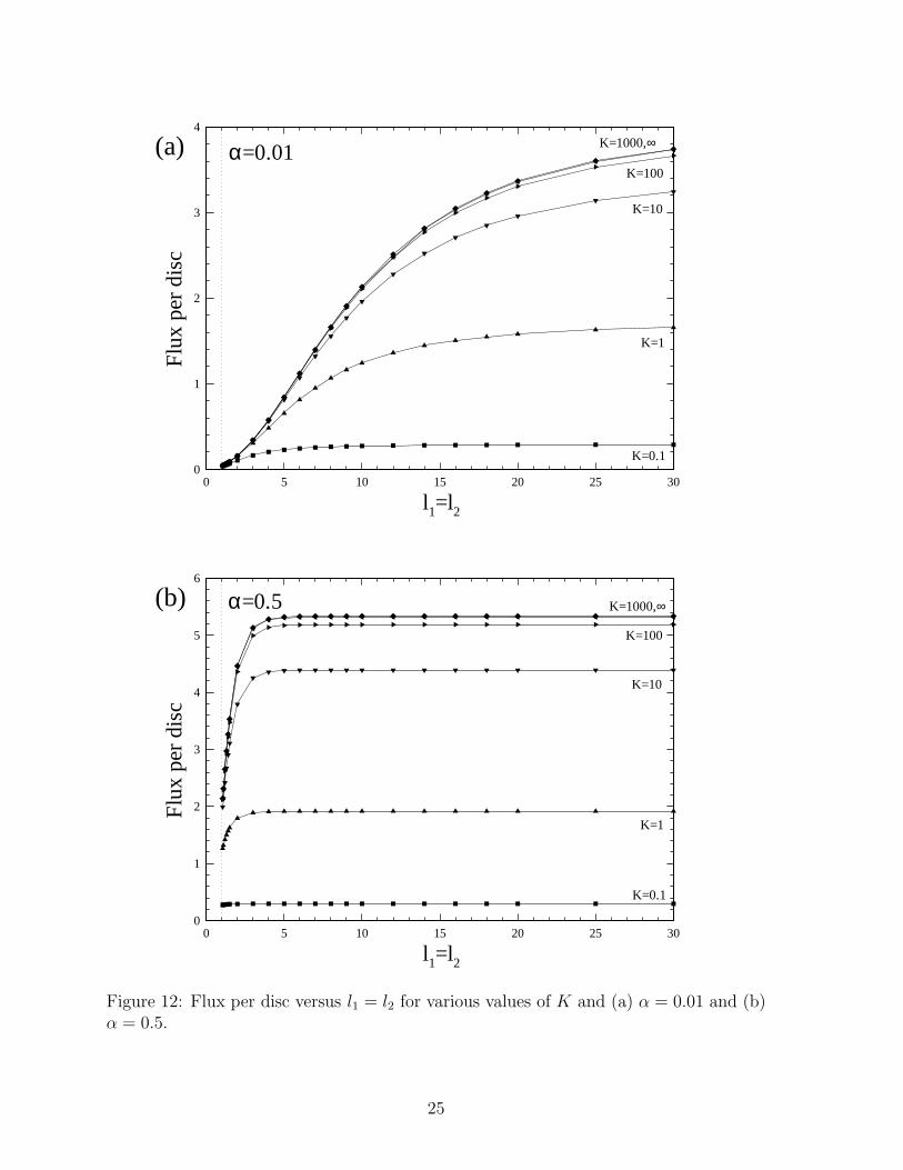
With the enormous range of parameters available, we choose to present in Figure12 the flux per disc versus l1 = l2 results for α = 0.01 and α = 0.5 for various K.The results for K = ∞ from Figure 7 are included to show the upper bounds on thepossible flux per disc in these cases. For small K, the curves of flux per disc versusl1 = l2 reach a steady state more quickly than for higher K. We can also see that forK > 100, there is very little difference in flux per disc compared to the K = ∞ case.If for physical systems there is a cost involved in increasing the surface reaction rateK of the electrodes, then there is a break even point at which increases in K result inincreases in flux per disc that are uneconomical. Also, for particular α, l1, l2, a value ofK can be found at which the flux per disc is any given percentage of the K = ∞ result.

5 Conclusion

Bender and Stone [5] developed an integral equation approach to the single disc steadystate microelectrode problem, and produced results of greater accuracy and flexibility(e.g. not limited to the pure diffusion, α = 0, case) than previously available. A com-bined eigenfunction expansion and boundary collocation approach was recently describedby Fransaer et al. [11], who also treated a finite number of electrodes. Here, we haveextended those results to the periodic microelectrode problem, and have investigatedthe effects of varying the periodic cell size. By allowing the flux φ′ to vary in both r andθ directions and using a periodic Green’s function, we have obtained results for periodicsystems, and have obtained results over a range of α and K values.

There are a number of possible simple extensions of the techniques presented here forfurther analysis. The problem of a ring microelectrode, or indeed any other potentiallyinteresting shape, can be modelled in both the single and periodic cases. For situationswhere we wish to maximize the flux per unit area from a periodic array, while minimizingthe quantity of microelectrode material placed on the plane, ring electrodes may indeedby more useful than discs. Also, the problem of random positioning of microelectrodeson a surface may be simulated by a periodic cell containing a random collection ofmicroelectrodes, random in both position and/or size.

Acknowledgments

We gratefully acknowledge NSF-PYI Award CT5-8957043 (to HAS) and the MERCK Foun-dation for funding this study. We thank Professors Ali Nadim and Ashok Sangani for helpfulconversations and discussions concerning Ewald sums. We would also like to thank the refer-ees for their helpful suggestions. This research was undertaken when SKL was a postdoctoralresearch fellow at Harvard University, under HAS.

24

0 5 10 15 20 25 300

1

2

3

4

l1=l2

Flu

x pe

r di

sc(a) α=0.01

K=1

K=0.1

K=10

K=100

K=1000,∞

0 5 10 15 20 25 300

1

2

3

4

5

6

l1=l2

Flu

x pe

r di

sc

(b) α=0.5

K=0.1

K=10

K=1

K=100

K=1000,∞

Figure 12: Flux per disc versus l1 = l2 for various values of K and (a) α = 0.01 and (b)α = 0.5.

25

References

[1] M. Abramowitz and I. A. Stegun, Handbook of Mathematical Functions, Dover, New York,1972.

[2] K. Aoki, K. Tokuda and H. Matsuda, Theory of stationary current-potential curves at mi-

crodisk electrodes for quasi-reversible and totally irreversible electrode reactions, J. Elec-troanal. Chem., 235 (1987), pp. 87–96.

[3] G. Balgi, D.E. Leckband and J.M. Nitsche, Transport effects on the kinetics of protein-

surface binding, preprint, 1995.

[4] G. Barton, Elements of Green’s Functions and Propagation, Oxford University Press,1989.

[5] M.A. Bender and H.A. Stone, An integral equation approach to the study of the steady

state current at surface microelectrodes, J. Electroanal. Chem., 351 (1993), pp. 29–55.

[6] A.M. Bond, K.B. Oldham and C.G. Zoski, Theory of electrochemical processes at an inlaid

microelectrode under steady-state conditions, J. Electroanal. Chem., 245 (1988), pp. 71–104.

[7] R.T. Bonnecaze and J.F. Brady, A method for determining the effective conductivity of

dispersions of particles, Proc. R. Soc. Lond. A, 430 (1990), pp. 285–313.

[8] C.A. Brebbia, J.C.F. Telles and L.C. Wrobel, Boundary Element Techniques: Theory and

Applications in Engineering, Springer-Verlag, Berlin, 1984.

[9] M. Fleischmann, S. Bandyopadhyay and S. Pons, The behaviour of microring electrodes,J. Phys. Chem., 89 (1985), pp. 5537–5541.

[10] M. Fleischmann and S. Pons, The behaviour of microdisk and microring electrodes, J.Electroanal. Chem., 222 (1987), pp. 107–115.

[11] J. Fransaer, J.P. Celis and J.R. Roos, Variations in the flow of current to disk electrodes

caused by particles, J. Electroanal. Chem., 391 (1995), pp. 11–28.

[12] I.S. Gradshteyn and I.M. Ryzhik, Table of Integrals, Series and Products, Academic Press,Boston, 5th ed., 1994.

[13] J.F. Hart, Computer Approximations, Wiley, New York, 1968.

[14] J.D. Jackson, Classical Electrodynamics, Wiley, New York, 1962.

[15] D.K. Kahaner and O.W. Rechard, TWODQD an adaptive routine for two-dimensional

integration, J. Comp. Appl. Math., 17 (1987), pp. 215–234.

[16] D.-Y. Kuan, H.T. Davis and R. Aris, Effectiveness of catalytic archipelagos. I regular

arrays of regular islands, Chem. Eng. Science, 38 (1983), pp. 719–732.

[17] D.-Y. Kuan, R. Aris and H.T. Davis, Effectiveness of catalytic archipelagos. II random

arrays of random islands, Chem. Eng. Science, 38 (1983), pp. 1569–1579.

[18] J.C. Lachat and J.O. Watson, Effective numerical treatment of boundary integral equa-

tions: a formulation for three-dimensional elastostatics, Int. J. num. Meth. Eng., 10(1976), pp. 991–1005.

[19] T.E. Mallouk, Minituarized electrochemistry, Nature, 343 (1990), pp. 515–516.

26

[20] S.J. Miklavic, D.Y.C. Chan, L.R. White and T.W. Healy, Double layer forces between

heterogeneous charged surfaces, J. Phys. Chem., 98 (1994), pp. 9022–9032.

[21] J. Newman, Resistance for flow of current to a disk, J. Electrochem. Soc., 112 (1966), pp.501-502.

[22] B.R.A. Nijboer and F.W. De Wette, On the calculation of lattice sums, Physica, 23 (1957),pp. 309–321.

[23] K.B. Oldham and C.G. Zoski, Comparisons of voltammetric steady states at hemispherical

and disc microelectrodes, J. Electroanal. Chem., 256 (1988), pp. 11–19.

[24] C.G. Phillips, The steady-state current for a microelectrode near diffusion-limited condi-

tions, J. Electroanal. Chem., 291 (1990), pp. 251–256.

[25] C.G. Phillips, The steady, diffusion-limited current at a disk microelectrode with a first

order EC’ reaction, J. Electroanal. Chem., 296 (1990), pp. 255–258.

[26] C.G. Phillips, The steady current for monticulate microelectrodes and assemblies of ultra-

microelectrodes, J. Electrochem. Soc., 139 (1992), pp. 2222–2230.

[27] C.G. Phillips and H.A. Stone, The steady-state current for a ring-like microelectrode under

non-diffusion-controlled conditions, J. Electroanal. Chem., to appear (1995).

[28] W.H. Press, B.P. Flannery, S.A. Teukolsky and W.T. Vetterling, Numerical Recipes: The

Art of Scientific Computing, Cambridge University Press, 1989.

[29] P.A. Ramachandran, Boundary Element Methods in Transport Phenomena, Computa-tional Mechanics Publications, Southampton, 1994.

[30] H. Reller, E. Kirowa-Eisner and E. Gileadi, Ensembles of microelectrodes, a digital simu-

lation, J. Electroanal. Chem., 138 (1982), pp. 65–77.

[31] A.S. Sangani and R. Sureshkumar, Linear acoustic properties of bubbly liquids near natural

frequency of bubbles using numerical simulations, J. Fluid Mech., 252 (1993), pp. 239-264.

[32] B.R. Scharifker, Diffusion to ensembles of microelectrodes, J. Electroanal. Chem., 240(1988), pp. 61–76.

[33] A. Szabo, Theory of the current at microelectrodes, applications to ring electrodes, J. Phys.Chem., 91 (1987), pp. 3108–3111.

[34] P.W. Voorhees and M.E. Glicksman, Solution to the multi-particle diffusion problem with

applications to Ostwald ripening - I. theory, Acta metall., 32 (1984), pp. 2001–2011.

[35] R.M. Wightman and D.O. Wipf, Voltammetry at ultramicroelectrodes, Electroanal. Chem.,15 (1989), pp. 267–353.

[36] IMSL MATH/LIBRARY Special Functions Version 2.0 (FORTRAN subroutines for math-ematical applications), IMSL, Houston, 1991.

27