An integral evaluation of dieselisation policies for households’ cars

Energy Policy 39 (2011) 5228–5242

Contents lists available at ScienceDirect

Energy Policy

0301-42

doi:10.1

n Tel.:

E-m1 I

comme

present2 Se

pdf.3 Se

journal homepage: www.elsevier.com/locate/enpol

An integral evaluation of dieselisation policies for households’ cars

Miguel A. Tovar n,1

Department of Economics, University of Essex, Wivenhoe Park, Colchester, Essex CO4 3SQ, United Kingdom

a r t i c l e i n f o

Article history:

Received 1 November 2010

Accepted 23 May 2011Available online 16 June 2011

Keywords:

Car passenger

Fuel demand

Diesel penetration

15/$ - see front matter & 2011 Elsevier Ltd. A

016/j.enpol.2011.05.041

þ44 1206874373; fax: þ44 1206 87 2724.

ail address: [email protected]

am grateful to two referees and Dr. Emm

nts. All the remaining mistakes are my own.

ed in the 3er ELAEE conference.

e OECD Annual Report 2009. www.oecd.or

e Schipper (2009).

a b s t r a c t

Reducing energy consumption and CO2 emissions in the transport sector is a priority for Great Britain

and other European countries as part of their agreements made in the Kyoto protocol and the Voluntary

Agreement. To achieve these goals, it has been proposed to increase the market share of diesel vehicles

which are more efficient than petrol ones. Based on partial approaches, previous research concluded

that increasing the share of diesel vehicles will decrease CO2 emissions (see Al-Hinti et al., 2007; Jeong

et al., 2009; Zervas, 2006). Unlike these approaches, I use an integral approach based on discrete choice

models to analyse diesel vehicle penetration in a broader context of transport in Great Britain. I provide

for the first time, empirical evidence which is in line with Bonilla’s (2009) argument that only

improvements in vehicle efficiency will not be enough to achieve their goals of mitigation of energy

consumption and CO2 emissions. The model shows the technical limitations that the penetration of

diesel vehicles faces and that a combination of improvements in public transportation and taxes on fuel

prices is the most effective policy combination to reduce the total amount of energy consumption and

CO2 emissions among the analysed dieselisation polices.

& 2011 Elsevier Ltd. All rights reserved.

1. Introduction

Great Britain along with other European countries needs todesign policies to reduce the amount of emissions of carbondioxide (CO2) and other pollutants as part of their obligationsacquired in the Kyoto protocol and the Voluntary Agreement forthe European Union (EU). The transport sector contributes 30% ofthe total CO2 emissions and it accounts for 60% of the total oilconsumption in the OECD countries.2 For this reason policymakers and researchers believe that more CO2 emissions can besaved from the transport sector. Nevertheless there is no agree-ment about the mechanism that can lead to reduced energyconsumption and CO2 emissions.3 One of the strategies to achievethese goals is to increase energy efficiency in the sector. For thisreason increasing diesel vehicles has been proposed as a strategygiven that these vehicles are more efficient than the petrol ones.However, it is important to mention that reducing CO2 emission isnot the only relevant goal that the transport sector aims toachieve. With regard to this, Bonilla (2009) pointed out that evenwhen the average fuel efficiency is improved, environmental

ll rights reserved.

a Iglesias for their helpful

A version of this paper was

g/dataoecd/38/39/43125523.

problems can be aggravated. For example diesel cars are moreefficient than petrol ones but they have also a higher emission ofparticulates which are another dangerous form of pollution.

According to Bonilla (2009), increasing the share of dieselvehicles in Great Britain and therefore the average fuel economy4

is achievable only in the long run and can be driven by incomeand car prices. In the case of Korea, Lee and Cho (2009) estimatethe future demand of diesel vehicles, finding that consumerswould increase the demand of those vehicles if the price of dieselwere relatively cheaper than petrol. Kim et al. (2006) found thatchanges in diesel price can be an effective policy to make changesin the share of diesel vehicles in the total vehicle stock. It isunclear however, if only increasing the number of diesel vehiclescan solve the problem of reducing energy consumption and themitigation of green house gases. Regarding this, Al-Hinti et al.(2007) found that increasing the number of diesel cars in Jordan’seconomy reduced the amount of energy consumption and CO2

emissions. Jeong et al. (2009) analysed the effect of introducingdiesel vehicles in the Korean economy. They found that increasingthe number of diesel vehicles has decreased carbon emissions butit also has increased the general amount of pollutants. Similarresults were found for Ireland by Zervas (2006).

On the other hand, based on analysis of improvements in theefficiency of new vehicles in the UK, Bonilla (2009) concluded thatit is likely that the EU environmental agreements will not be

4 The average fuel economy is the average of the ratio between distance

travelled and energy consumed.

www.elsevier.com/locate/enpol

dx.doi.org/10.1016/j.enpol.2011.05.041

mailto:[email protected]

www.oecd.org/dataoecd/38/39/43125523.pdf





dx.doi.org/10.1016/j.enpol.2011.05.041

M.A. Tovar / Energy Policy 39 (2011) 5228–5242 5229

reached given that these improvements are not sufficient. The factthat improvements in energy efficiency fail to reach their goalscan be attributed to a rebound effect. According to Frondel et al.(2007) having more efficient vehicles can make energy usecheaper and therefore it can increase its consumption. SimilarlySchipper and Fulton (2009) noted that the rebound effect can havethree sources: (1) an increase in the number of diesel cars as aresult of petrol drivers switching to diesel cars to drive more,(2) an increase in the intensity of using diesel cars from ownerswho already own these vehicles, and (3) an increase in thenumber of bigger and heavier vehicles. Moreover, Schipper et al.(2002) argue that on average a decrease in 10% of the price oftravelling could induce an increase in the demand of travelling of5% (i.e. an elasticity of 0.5). However, they argued that in Europethis effect can be higher given that commuters have moreflexibility to switch from public transportation to car when theprice of travelling by car is reduced.

The demand of diesel cars tend to be focused on big vehiclesand as noted by Cuenot (2009) there is a correlation betweenweight and CO2 emissions, and therefore possible gains comingfrom fuel efficiency can be offset by the weight of diesel vehicles.Bonilla and Foxon (2009) found that people with high incometend to buy larger diesel cars which increases fuel consumption.In the same vein, Schipper and Fulton (2009) noted that there is aself selection process in the purchase of diesel vehicles.5 More-over, they argued that it is important to identify the determinantsof this process given that they play also an important role in theuse of these vehicles. Therefore, how to introduce more efficientvehicles in the economy is still an unanswered question. More-over, modelling dieselisation of the vehicle stock requires anintegral approach that allows the evaluation of improvements ofefficiency and changes in commuter preferences in a broadercontext of transport. In this sense, all previously mentionedstudies visualise diesel vehicle penetration as an isolated phe-nomenon, and therefore this limits the analysis. The objective ofthis paper is to improve the modelling approach providing anintegral analysis that will bring new evidence of the effect ofimproving the average fuel efficiency on energy consumption andCO2 emissions by an increase in the number of diesel vehicles.Moreover, the model is able to analyse different dieselisationpolicies based on changes in fuel prices and improvements ofpublic transportation.

Integral approaches have been used by Mohammadian andMiller (2003) to estimate vehicle ownership and type of vehicledecision. More recently Chiou et al. (2009) analysed changes inenergy and emissions based on integrated model that follows a‘‘bottom up style’’ where several modules such as vehicle own-ership, type of vehicle and usage are linked through technicalprinciples to estimate changes in energy consumption and emis-sions. The model was applied to a Korean survey that was carriedout in 2006. While their objective was not to analyse dieselvehicle penetration, this structure allowed them to have a broadervision of the effects that changes in preferences of drivers fordifferent car type models and usage have on energy consumptionand green house emissions.

In this paper, diesel vehicle penetration is analysed by expand-ing Chiou et al’s. (2009) model to be applied to a repeated crosssection dataset that allows the study of changes across time. UnlikeChiou et al. (2009), the model proposed here comprises twoadditional modules. One for travel mode to analyse commuter’sbehaviour and other for newly acquired vehicles. This allows the

5 The authors argue that given that the cost for diesel cars is higher than for

petrol ones, purchasers have an idea of the number of miles that they have to drive

to make the investment profitable when they buy a diesel car.

effects on energy consumption and CO2 emissions of improvementsin public transportation to be included. In addition, the ownershipmodule is estimated in a two stage approach. This structure allowsanalysis of the effect of improvements in public transportationalong with changes in diesel vehicle penetration on energy con-sumption and CO2 emissions. However, given limited informationabout usage and efficiencies of other transport modalities, themodel estimates only energy consumption and CO2 emissioncoming from households’ cars.6 My model also distinguishes Big

cities from the rest of Great Britain to analyse possible regionaleffects. The estimation is based on the National Travel Survey (NTS)for the case of Great Britain from 1998 to 2006. The NTS carries outa survey of household transport behaviour in the UK. The datasetreports information in different dimensions such as transport mode,vehicle type and usage choice.

The model shows evidence that diesel vehicle penetration facestechnical limitations given that these vehicles are more likely to bepurchased by male consumers with high income and with prefer-ences for heavy vehicles. Therefore manufactures face a doublechallenge: they need to make these vehicles lighter and accessibleto different kind of driver regardless of gender or socioeconomic leveland at the same time improve fuel efficiency. Moreover the modelprovides empirical evidence that increasing the number of diesel carsby either a reduction in diesel price or an increase in diesel fuelefficiency does not decrease energy consumption or CO2 emissions.This effect is attributed to fact that these policies also increase theusage of diesel vehicles prompting a rebound effect as found byFrondel et al. (2007) and Schipper and Fulton (2009). Therefore, incontrast to Al-Hinti et al. (2007), Jeong et al. (2009), and Zervas(2006), increasing the diesel vehicle penetration alone will notprovide mitigation effects on energy consumption and CO2 emis-sions. These findings support Bonilla (2009)’s argument that increas-ing the number of diesel vehicles will not be enough to achieve GreatBritain’s environmental compromises. Nevertheless the combinationof introducing vehicle efficiency via taxing petrol cars along withimprovements in public transportation induces the highest reductionin energy consumption and emissions of CO2 from households’ cars.

My model presents several advantages over partial approachesand studies based on time series techniques. Vaage (2000) arguedthat time series techniques use aggregate data that omits manyimportant characteristics of households. Consequently this canlead to missing variables and potentially, to mis-specificationbias. In addition, aggregate results do not allow authorities toevaluate the effect of policies across households. This paperovercomes these problems using cross section data combinedwith discrete choice models. In addition, the model provides asfar as I know the first empirical evidence of the effects of differentdieselisation policies based on a very tractable structure thatallows analyses of different aspects of the transportation sector.

The paper comprises five sections. Section 2 describes theeconometric techniques used and the details of how the modulesare linked. The subsequent two sections explain the dataset used andthe econometric results. The forth and the fifth sections provide theresults of the policies experiments and conclusions, respectively.

2. The model and methodology

2.1. The general structure

The model is a modular estimation that comprises five mod-ules linked through technical factors. The first module estimates

6 The structure of the model makes it possible to estimate energy consump-

tion and CO2 emission from other modalities of transportation provided that the

information is available.

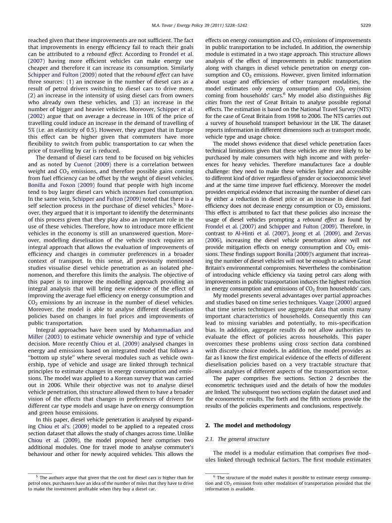
Fig. 1. Integrated structure.

M.A. Tovar / Energy Policy 39 (2011) 5228–52425230

the elements that determine the commuter’s decision for trans-port mode, from now on denoted as m1. Module 2, estimates thehousehold’s decision of how many cars to own (m2). The thirdmodule analyses the individual decision of vehicle type (m3),while m4 estimates changes in the vehicle stock, and finallymodule 5 (m5) estimates the annual kilometres that vehicles areused. The model structure is shown in Fig. 1.

Chiou et al. (2009) estimate the sensitivity of commuters tochanges in transport cost using a stated preference methodol-ogy7; however, the NTS dataset is not designed to allow for thiskind of estimation. Therefore m1 is added to estimate thesensitivity of commuters to changes in transport modes prices.This fact, unlike Chiou et al. (2009), allows the model to accom-modate for changes in prices and other factors that determinecommuters’ decisions about mode of travel.

In the second module (m2) the total number of vehicles isestimated based on the total number of British households and

7 According to Azevedo et al. (2003), revealed preferences estimation is based

on factual information while a stated preferences one is based on the possible

reaction of demand to hypothetical changes in prices.

the probability of vehicle ownership. The total number of vehiclesis disaggregated using Multinomial Logistic Models estimated inm3. It provides the shares needed to disaggregate the vehiclestock by fuel and age. New purchases of vehicles are estimated inmodule 4 using an ordered probit model. Finally, the intensity ofvehicle usage is estimated in m5 where the annual kilometres canbe disaggregated by type and age of vehicle. Once the number ofvehicles per different categories is multiplied by the annualkilometres, it is straight forward to estimate energy consumptionand emissions. This is carried out using the average amount offuel consumption per kilometre and emission factors provided bythe Department of Transport.8 Emission factors are broken downby vintage, fuel and engine capacity and therefore real sharestaken from the NTS are used to disaggregate the vehicle stock atengine capacity level.

To introduce changes in commuter preferences, changes in m1are transmitted to the model by the ratio of probabilities of

8 Tables 1 and 3 show factors of efficiency and emissions used in this estimation.

These estimates are available at http://www.dft.gov.uk/pgr/statistics/datatablespu

blications/energyenvironment/ and http://www.dft.gov.uk/pgr/roads/environment/

emissions/.

http://www.dft.gov.uk/pgr/statistics/datatablespublications/energyenvironment/

http://www.dft.gov.uk/pgr/statistics/datatablespublications/energyenvironment/

http://www.dft.gov.uk/pgr/roads/environment/emissions/


9 See Train (2003).10 See Heckman (1979) and Frondel and Vance (2010).11 Cameron and Trivedi (2005) note that the estimated probabilities from logit

and probit models are very similar.


travelling by car, where pm1car is the probability that an individual

chooses to travel by car in region h at time t and it is estimated inm1. In pm1

car ð1Þ=pm1car ð0Þ the base scenario (0) and an alternative

scenario (1) are compared. The alternative one represents, forinstance, changes in prices of public transportation via subsidies.More details are provided in the next sections.

2.2. Mode transport module

The first module m1, presents five options for commuters:walking, bicycle, car, motorcycle, bus and train. The estimation ofpm1

carht is carried out using a Conditional Multinomial Logit model(CML). The model is interpreted in the framework of RandomUtility Models (RUM). The model follows the next specificationwhere for simplicity the subscript for individuals is omitted:

Ujht ¼ xm10

jht bm1þzm10

ht gm1j þe

m1jht , ð1Þ

where Ujh is the utility for alternative j in region h at time t whichis not observable. Moreover, xm1

jt is the vector of alternative-specific variables while zm1

ht comprises the case-specific variables.Therefore, the probability of choosing alternative j in region h attime t is estimated by

pht ¼expðxm10

jht bm1þzm10

ht gm1j ÞPJ

l ¼ 1 expðxm10

lht bm1þzm10

ht gm1l Þ

, ð2Þ

and j¼1, y J, t¼1, y, T, and h¼1, y, H. In this framework, theerror terms em1

jht are assumed to be independent and identicallydistributed (iid). Therefore, when an individual is comparing twoalternatives, the addition of a new one does not affect thedistribution of the probability that the individual attributes tothe two initial alternatives. That is, ejht, does not contain anyalternative-specific unobservable information.

The previous property is technically called the Independencefrom Irrelevant Alternatives (IIA). In some situations this propertycannot be a realistic representation. Nevertheless, it can berelaxed assuming that ejht can be correlated across alternatives.Ben-Akiva (1974) introduced a Nested Multinomial Logit (NML)that relaxes the IIA assumption. In m1 commuters face a twolevels tree of decision. In the first level, commuters choosebetween travelling by non motorised mode, private motorisedand public motorised which are called limbs j by Cameron andTrivedi (2009) while the elements that belong to each limb arecalled branches denoted as k. The first nest or branch comprisesthe choices walking and cycling, the second one car and motor-cycle and the third one bus and train. In this structure theprobability that a commuter in region h at time t travels by caris denoted as p21ht. Subscript 21 denotes second limb (privatemotorised) and first choice (car) in the branch. The probability ofchoosing an alternative k within a branch that belong to limb j isestimated as follows:

pjkht ¼ pjhtpk=jht ¼expðv0jhtaþtjIjhtÞPj

n ¼ 1 expðv0nhtaþtnInhtÞ

�expðx0jkhtbj=tjÞPk

l ¼ 1 expðx0jlhtbj=tjÞ, ð3Þ

where the vector vjht comprises all the variables that only variesacross individuals, limbs region and time while the vector xjkht

comprises the variables that vary across all the subscripts. Notethat xjkht in this procedure and xm1

jht in the CML, contains the sameinformation the only difference is that in the nested method theelements of xm1

jht are divided into k groups.The variable Ijht is the inclusive value. The economic intuition

is that once the individuals choose the alternative at the bottomlevel, then the information of this utility is brought back to the

highest level through the inclusive value. It is defined as

Ijht ¼ lnXkj

l ¼ 1

expðx0lhtbj=tjÞ

24

35: ð4Þ

Moreover, tj is called the dissimilarity parameter and its valuemust be between zero and one. 1�tj will provide informationabout the correlation across alternatives in a nest.9 FollowingChiou et al. (2009) methodology, when tj is found to be out of itsrange, then a conditional logit model is used instead. A caveat oflogit models is the assumption of proportionality in the pattern ofsubstitution. Possible alternatives are Multinomial Probit modelsand Cross-Nested logits which can capture flexible patterns ofsubstitution. However, when either the dataset or the number ofalternatives is very large, as in my estimation of transport modeand vehicle type, estimation of the parameters become a compu-tational burden. As noted by Chiou et al. (2009), the estimation ofthe parameters using those models can be extremely severeunder these circumstances.

2.3. Ownership module

The UK vehicle ownership has been analysed by Dargay andHanly (2004b) applying ordered probit models. Their strategy wasto estimate the probability of owning s vehicles where s takesvalues from zero to three. The authors used the British PanelSurvey which does not include any variable of vehicle price andtherefore it was needed either to impute zero prices or allowingfor missing values for the households that own zero vehicles.Even though in their paper it is not explicit the way that theproblem was solved, according to Frondel and Vance (2010) inthis situation a two stage procedure is more appropriate giventhat there is a sample selection problem. In the first step a probitmodel is estimated to control for the sample selection problemprompted by the zero cases.

In this paper I follow Frondel and Vance (2010) philosophywhere in the first step a probit model is estimated to compute theprobability of being a vehicle owner. For the second stage, insteadof estimating another model for the number of vehicles owned byhouseholds I use real actual shares for owning s cars, where s¼1,2,3 or more vehicles. The product of the probabilities obtainedfrom the first stage and these shares provide an estimate of pm2

sht:

Therefore for the first stage Um2ht 4Um2

ht if household in region h at

time t owns a car. Where Um2ht and Um2

ht denote the utility of car

owners and non car owners. Therefore, the probability is esti-mated as follows:

PrðUm2ht 4Um2

ht Þ ¼ Fðxm20

ht bÞ, ð5Þ

where F(n) is a cumulative distribution function for the errorterms. The most common functions are the normal and logistic.When the normal function is specified the model is called probit.The predicted probabilities from both models are very similar.However, for a self selection stage it is very common to find in theliterature the use of probit models.10 Therefore, I use a probitmodel for the policy evaluation section.11 Consequently, for thesecond decision, real shares from the NTS are used as follows:

pm2sht ¼ PrðUm2

ht 4Um2ht Þ � Shares of owning s cars ð6Þ

with this specification changes in PrðUm2ht 4Um2

ht Þ will modify theprobability of owning s vehicles in region h at time t.


2.4. Vehicle type and availability

This module estimates the probability of choosing a car type g inregion h at time t denoted as pm3

ght . As shown in Fig. 1, this module isdesigned to give individuals eight choices of vehicles. The choicesare a result of the combination of different car type models and fueltype. The car type models options are as follows: up to 1 year, from1 to 3, from 3 to 5, and over 5 while the fuel choices are eitherpetrol or diesel vehicles. The estimation is carried out using CML

and NML models as in module 1 following expressions (2) and (3).Nevertheless, in this module the decision tree that drivers face hastwo limbs, one for petrol and other for diesel vehicles. The branchesin each limb represent different choices of car type models.

On the other hand, to estimate the new purchases of vehiclesthe NTS provides information about the vehicle availability

recorded in three answers: (1) vehicle in regular use, (2) possiblywill come into use, and (3) newly acquired vehicle. The lastanswer is particularly interesting given that I can estimate thechanges in the probability of buying a diesel car given changes ineither fuel or car prices of those vehicles. Therefore, the indivi-dual’s answer to the question of vehicle availability can be seen asthe utility that the individuals attribute to each answer accordingto their ratings (see e.g. Train, 2003). Consequently, the prob-ability that an individual chooses alternative a (i.e. the values thatvehicle availability takes) for vehicle type g is estimated using anordered probit model.

I assume that the unobservable utility function denoted asUm4n

ght is contained in the interval (Za�1,Za], where Za�1,Za arethreshold values. Therefore the probability that householdschoose alternative a is given by

PrðUm4ght ¼ aghÞ ¼ PrðZa�1oUm4n

ght rZaÞ ¼ PðUm4nght rZaÞ�PðUm4n

ght rZa�1Þ

¼ FðZa�xm4’ght b

m4Þ�FðZa�1�xm40

ght bm4Þ, a¼ 1,2,3, ð7Þ

where xm4ght comprises all the independent variables such as fuel

and car prices and household’s characteristics. F(n) is the cumu-lative distribution function of the error terms. This function canbe specified to be logistic or normal. If it is specified as normal,the model used is called probit. However note that the logitmodel unlike the probit assumes independency between the errorterms and the alternatives. Consequently this assumption cannotbe realistic given the ordered nature of the variable vehicle

availability.12 Therefore the predicted probabilities are estimatedby a probit model in the simulation experiment.

2.5. Energy consumption and emissions

The total number of households that own s vehicles at time t inregion h is estimated by the following expression:

NHsht ¼ ðpm2sht NhtÞ, ð8Þ

where Nht13 is the total number of households in region h at time t.

Once this decision is made, commuters can choose the kind ofcar that they want to buy. Fig. 1 shows that they can choose twogeneral options: petrol or diesel vehicles for different car typemodels. The probability of choosing a vehicle of type g in region h

at time t is denoted as pm3ght . It is estimated using CML and NML. To

compute the number of vehicles of type g in region h at time t (i.e.TVght), first the total number of vehicles TV in region h at time t are

12 See Train (2003).13 See Table 1 for details on the number of households.

estimated as follows:

TVht ¼X4

s ¼ 1

NHsht s, ð9Þ

where s takes values from 1 to 4 denoting the number of cars thathouseholds can own. TVght is computed by expression (10) asfollows:

TVght ¼ TVht pm3ght , ð10Þ

where pm3ght is the probability of owning a car type g in region h at

time t estimated in m3. Moreover g¼1, 2, y, G.The introduction of new vehicles is estimated in module 4 by

expression (7), particularly by changes in the probability fornewly acquired vehicle. Therefore under an alternative scenario(i.e. a reduction of diesel price), TVght is multiplied by thedifference in expression (7) with respect to the base scenario asfollows:

TVghtð1þDPrðUm4ght ¼ newly acquired vehiclesÞÞ,

where DPrðUm4ght ¼ newly acquired vehiclesÞ is the change in the

probability of new acquired vehicle for a given change in fuel orcar prices.

Regarding the annual kilometres that vehicle g is used (i.e.usageght), it is estimated in module 5 by the following expression:

lnYght ¼ Xm5ghtb

m5þeht , ð11Þ

where lnYght is the logarithm of the annual kilometres of anindividual in region h at time t of the g type, eght is the error termand X5m

ght is the matrix with all the independent variables. Morespecific details of the variable used in the estimation are providedin the next section. The model is estimated by Pooled OrdinaryLeast Squares (POLS). Note that usageght is estimated as theexponential function from (11).

On the other hand, the total kilometres (i.e. TMght) by car typeg in region h at time t is estimated by the following expression:

TMght ¼ TVghtusageght

pm1carhtð1Þ

pm1carhtð0Þ

, ð12Þ

where pm1carhtð1Þ=pm1

carhtð0Þ measures the proportion of change in theprobability of travelling by car estimated in m1. It compares thescenario base (0) and the scenario of changes in bus prices (1).Note that in the base scenario pm1

carhtð1Þ=pm1carhtð0Þ ¼ 1: Fuel con-

sumption and emissions are estimated as follows:

FVght ¼ TMght=efficiencygt , ð13Þ

where efficiencygt is the fuel average consumption per mile in g

category at time t.The amount of CO2 emissions in region h at time t is computed

by the following expression14:

CO2ght ¼ TMght emission factors ð14Þ

3. Empirical results

3.1. The dataset

The dataset is provided by the National Travel Survey (NTS)and it comprises information at individual, household and vehiclelevel. The data is generated by an annual survey carried out in theUnited Kingdom. However, in this research only the case of GreatBritain is analysed. Moreover, only information of individuals

14 The emission factors are provided by car type model, fuel and engine

capacity as shown in Table 11. The vehicle stock was disaggregated by engine

capacity using shares from the NTS.


with age greater than 16 years is considered. This follows Dargayand Hanly (2004a) who only consider individuals with legal ageto drive in the UK. The estimation is carried out for T¼9 years(from 1998 to 2006) and it distinguishes two regions (H¼2), Big

cities and the rest of Great Britain. The variable Big cities com-prises London boroughs, met built-up areas and urban cities witha population of over 250 K. The rest of Great Britain is representedby cities with less than 250 K and rural areas. Three dummyvariables to identify three periods are included in the models.Period 1 comprises years from 1998 to 2000, Period 2 from 2001 to2003 and Period 3 from 2004 to 2006, this is done in order toreduce the number of parameters to be estimated.

The variables from the NTS used in the estimation are describedin Table 1. The letters in brackets (i.e. m1, m2, m3, m4, and m5)denote the modules where the variables are used. Note that thesample size of the survey has been increasing across periods. Thishas been done to increase the representativeness of the survey.15

Table 1 shows strong car dependence as the mean of thevariable Transport mode denotes that travelling by car is the mainmode of transport. This pattern remains unchangeable across theanalysed period. Moreover, the variable cars in the household havebeen increasing across the analysed period. This variable dependsas I will show later on Frequency of Buses. In addition, according toa survey carried out by the DfT non-bus-users could be encour-aged to use buses if punctuality and fares are improved.16

Nevertheless, variables such as Walk time to bus stop and Commute

cost which indicate improvements in these issues have notchanged significantly across the three analysed periods.

Regarding vehicle level, the variables Engine capacity andVehicle size show a tendency to buy more powerful and heavyvehicles which is contrary to any policy of mitigation as men-tioned by Cuenot (2009). In addition, Table 1 shows that the meanof the variable Usage is around 7 which in the survey this numberidentifies the range 4300–5600 annual km. This implies that thedaily distance driven in Great Britain (i.e. 12–15 km) has notchanged significantly across the period analysed.

Regarding diesel cars, the variable Fuel type shows that thesevehicles have seen a growing tendency across the analysed perioddespite of the fact of facing an annual average growth in dieselprices of 2%. Additionally unlike other European countries, in GreatBritain diesel is more expensive than petrol. Nevertheless, whatmakes diesel cars competitive is the gap in fuel Efficiency betweendiesel cars and petrol ones. This gap was high at the beginning ofthe analysed period; however, it is currently getting narrower.

Although the dataset covers a considerable range of variablesin the transport sector, there is a lack of information related tohousehold income and prices of transport mode and cars. For thisreason, the NTS dataset is complemented using public informa-tion provided by the Department for Transport (DfT) and theAutomobile Association (AA). The variable Commute cost is builtas follows. For the case of car price, the Automobile Associationprovides prices of driving per mile for diesel and petrol vehicles17

and an average is estimated and used as cost of this modality. Forbus and train prices, a cost is obtained from the NTS datasetwhere the total cost is divided by total distance travelled to get anestimation for the cost of travelling per mile. Finally, the cost ofwalking and cycling is set equal to zero.18

15 The manual that accompanies the dataset specifies that there are no major

changes of the survey methodology across years apart from omission of some

variables. Therefore pooling the data from these years is possible.16 Public experiences and attitudes towards bus travel 2009.17 See Moring Cost provided by the Automobile Association available at http://

www.theaa.com/motoring_advice/running_costs/archive.html.18 See Hole and FitzRoy (2004).

Improvements in public transportation to reduce the waitingtime of commuters can be achieved by either making bus servicesmore efficient or increasing the number of buses. Moreover, theeffect of an increase in the number of buses in a region will berelative to each commuter’s perception of Bus frequency which isreported in the NTS. Therefore, to analyse the effect of improve-ments in public transportation, I introduce the variable Bus

availability which is estimated by multiplying Bus frequency andthe number of buses in the region.19. This will allow me toevaluate the commuter’s response of vehicle ownership tochanges in the number of buses. However note that this modelonly estimates changes in energy consumption and CO2 emissionscoming from households’ cars.

In discrete choice models it is common practice to normaliseprices by an income variable.20 Therefore the higher the indivi-dual’s income, the smaller weight that those prices receive forthose individuals. However, as previously mentioned, to intro-duce the effect of income in the estimations is complicated giventhat there is a lack of consistency across the years in the survey inthis variable. Hence the variable socioeconomic level is used asproxy in the econometric specifications. The nature of thisvariable (bounded between 0 and 5) makes it to work better insome estimations than in others. Note, however, that othervariables such as Cars in the household, distance travelled, number

of owned cars and fuel consumed can be indicators of the house-hold’s income level. The criterion to choose among these variablesin the econometric specification is based not only on statisticalsignificance but also on accordance with economic theory. Forinstance, the variable Car price and fuel price are weighted by thevariable socioeconomic level in the module for type and age vehiclechoice while in the usage estimation car price is normalised by theamount of fuel consumed.

As previously mentioned, the structure of the model requirestaking into consideration vehicle age given that this determinesdistance travelled, fuel consumption and CO2 emissions. Hence toaccount for the fact that Car price changes according to the car’sage, the price is adjusted using the estimation of price variationcarried out by the Royal Automobile Club Foundation for Motor-ing.21 Moreover, Fuel price is divided by the vehicle Efficiency totake into consideration that drivers face relative prices accordingto the vintage and efficiency of their vehicles that change acrosstime. These variables are provided by the DfT in Transport

Statistics Great Britain 200822.To control for the fact that the degree of urbanisation plays an

important role in designing transport policies, I follow Frondeland Vance (2010) who introduced the variable Big cities. In myestimation the variable Big cities comprises London boroughs, metbuilt-up areas and urban cities with a population of over 250 K.The rest of Great Britain is represented by cities with less than250 K and rural areas. The next table shows some of the keyvariables broken down by these two regions. The columnsentitled Period show the absolute frequency whereas the columnsbeside show the relative frequency.23

Table 2 shows some important differences across regions. Onecan see that travelling by car is more popular in other cities than inBig cities. Consequently the use of public transportation is

19 Available at http://www.dft.gov.uk/pgr/statistics/datatablespublications/

vehicles/20 See Ben-Akiva and Lerman (1985). They include simultaneously in the

econometric specification, prices normalised by income and an income variable.

Therefore they are able to analyse jointly individual responses to relative prices

and income effects.21 See Transport Price Indices, 2009, http://www.racfoundation.org/.22 This version is available at http://www.dft.gov.uk/pgr/statistics/datatable

spublications/tsgb/.23 Absolute frequencies normalised by the total number of events.

http://www.theaa.com/motoring_advice/running_costs/archive.html

http://www.theaa.com/motoring_advice/running_costs/archive.html

http://www.dft.gov.uk/pgr/statistics/datatablespublications/vehicles/

http://www.dft.gov.uk/pgr/statistics/datatablespublications/vehicles/

http://www.racfoundation.org/

http://www.dft.gov.uk/pgr/statistics/datatablespublications/tsgb/

http://www.dft.gov.uk/pgr/statistics/datatablespublications/tsgb/

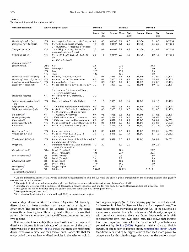
Table 1Variable definition and descriptive statistics.

Variable definition Source Range of values Period 1 Period 2 Period 3

Mean Std.

dev

Sample Mean Std.dev.

Sample Mean Std.dev.

Sample

Number of tranfers (m1) NTS 0¼1 stage,1,¼2 stages, y, 6¼6 stages 0.1 0.3 60,907 0.1 0.3 113,361 0.1 0.3 147,054

Purpose of travelling (m1) NTS 0¼work, 1¼ in course of work, 1.5 2.5 60,907 1.4 2.6 113,361 1.5 2.6 147,054

2¼education, 3¼shopping, 4¼holiday

Transport mode (m1) NTS 1¼walking or cycling, 2¼car, 3¼ 2.2 0.9 60,907 2.2 0.9 113,361 2.2 0.9 147,054

motorcycle, 4¼bus, 5¼train

Commuter age (m1) NTS 0¼16–19, 1¼20–29,2¼30–39,3¼40–

49

2.8 1.5 60,907 2.9 1.5 113,361 2.9 1.5 147,054

4¼50–59, 5¼60–69

Commute cost(m1)a

(Pence per km) Other Car 22.1 23.3 23.2

Other Motorcycle 16.1 17.1 17.0

NTS Bus 12.7 13.7 15.9

NTS Train 12.2 12.3 11.9

Number of owned cars (m4) NTS 0¼none, 1¼1,2¼2,3¼3,4¼4 1.0 0.8 7965 1.1 0.8 16,349 1.1 0.9 21,175

Number of owned bicycles (m1) NTS 0¼none, 1¼one, 2¼two or more 0.7 0.8 7965 0.7 0.8 16,349 0.8 0.8 21,175

Members with full licence(m4) NTS 0¼none,1¼1, y, 4¼4 1.3 0.9 7965 1.3 0.9 16,349 1.3 0.9 21,175

Frequency of buses(m2) NTS 0¼ less than once a day, 1¼once a day,

?.

3.0 1.0 7965 3.0 1.0 16,349 3.0 1.0 21,175

2¼1 an hour, 3¼1 every half hour,

4¼1 every quarter hour

Household size(m2) NTS 0¼1 member, 1¼2 members, y,

4¼five

2.2

Socioeconomic level (m1–m3,

m5)

NTS Five levels where 0 is the highest 1.5 1.3 7965 1.5 1.4 16,349 1.5 1.3 21,175

Employment (m3,m5) NTS 1¼full time employment, 0 otherwise 0.2 0.5 7965 0.2 0.5 16,349 0.2 0.5 21,175

Walk time to bus stop(m2) NTS 0¼6 min, 1¼7–13 min, 2¼14–26 min 0.2 0.5 7965 0.2 0.5 16,349 0.2 0.5 21,175

3¼27–43 min, 4¼44 min or more

Big cities(all)b NTS 1¼big cities, 0 otherwise 0.4 0.5 7965 0.4 0.5 16,349 0.5 0.5 21,175

Driver gender(m3) NTS 1 if the driver is male, 0 otherwise 0.6 0.5 8371 0.6 0.5 18,143 0.6 0.5 24,552

Property(m3) NTS 1 if the car is provided by a company 0.1 0.3 8371 0.1 0.2 18,143 0.0 0.2 24,552

Engine capacity(m3) NTS 0¼up to1500 and 1¼more than 1500 cc 0.6 0.5 8371 0.6 0.5 18,143 0.6 0.5 24,532

Car size(m3) NTS 0¼small,1¼medium, 2¼ large cars 1.4 1.3 8371 1.7 1.5 18,143 1.8 1.5 24,552

Fuel type (m3–m5) NTS 0¼petrol, 1¼diesel 0.1 0.3 8371 0.2 0.4 18,143 0.2 0.4 24,552

Vehicle age(m3–m5) NTS 0¼up to 1 year, 1¼1–2, 2¼2–3, 3.1 1.3 8371 3.0 1.4 18,143 3.1 1.3 24,552

3¼3–5, 4¼over 5 years

Vehicle availability(m3) NTS 0¼regular use, 1¼possibly will be used 0.0 0.2 8371 0.0 0.2 18,143 0.0 0.2 24,552

2¼new acquired vehicle

Usage (m5) NTS Minimum value 0¼312 and maximum 7.2 2.7 6.9 2.7 6.9 2.6

12¼18,750 annual km

Car price(m3–m5)c Other Petrol (Pence/km) 15.1 18.4 20.7

Diesel (Pence/km) 19.8 23.4 26.5

Fuel price(m3–m5)d DfT Petrol (Pence/l) 7.2 7.6 8.6

DfT Diesel (Pence/l) 7.4 7.8 8.9

Efficiency(m3–m5)e DfT Petrol (km/l) 12.2 12.7 13.2

DfT Diesel (km/l) 15.0 16.0 15.9

Density(m4)f Other km/per capita 0.7 0.7 0.7

Number of

household(simulation)s

DfT Millions 20,066 20,715 21,215

a Car and motorcycle prices are an average estimated using information from the AA while the price of public transportation are estimated dividing total journey

distance and cost from the NTS.b The variable Big cities includes London boroughs, met built-up areas and urban cities with a population of over 250 k.c Estimated average price that includes cost of depreciation, service, insurance cost and tax road and other costs. However, it does not include fuel cost.d Average for the period estimated using the price of unleaded petrol and ultra low sulphur diesel.e Average efficiency of new cars.f It is estimated by dividing the total road length (DfT) by population per region.


considerably inferior in other cities than in big cities. Additionally,diesel share has been growing across years and it is higher inother cities. The proportion of old vehicles is almost the sameacross these two regions. These regional differences show thatpotentially the same policy can have different outcomes in thesetwo regions.

It is important to identify the characteristics of the buyers ofdiesel cars because it is an indicator of the intensity of the use ofthese vehicles. In this sense Table 3 shows that there are more maledrivers who own a diesel car than female ones. Notice also that forevery period there are heavier diesel vehicles in the vehicle stock. In

both regions property (i.e. 1 if a company pays for the vehicle cost,0 otherwise) is higher for diesel vehicles than for the petrol ones. Thesame occurs also for the variable employment (i.e. 1 if the household’smain earner has a full time job, 0 otherwise). Additionally, comparedwith petrol cars owners, there are fewer households with highsocioeconomic level that own diesel cars. This shows that incomelevels are important drivers for the diesel vehicle penetration aspointed out by Bonilla (2009). Regarding Vehicle size and Vehicle

capacity, it can be seen as pointed out by Schipper and Fulton (2009)that diesel cars tend to be bigger vehicles that need more power tocompensate for this disadvantage. Moreover, as the authors noted

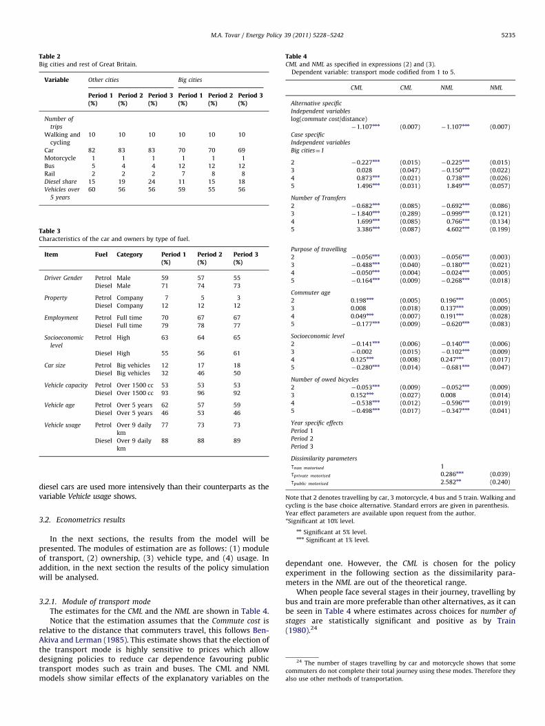
Table 3Characteristics of the car and owners by type of fuel.

Item Fuel Category Period 1(%)

Period 2(%)

Period 3(%)

Driver Gender Petrol Male 59 57 55

Diesel Male 71 74 73

Property Petrol Company 7 5 3

Diesel Company 12 12 12

Employment Petrol Full time 70 67 67

Diesel Full time 79 78 77

Socioeconomic

level

Petrol High 63 64 65

Diesel High 55 56 61

Car size Petrol Big vehicles 12 17 18

Diesel Big vehicles 32 46 50

Vehicle capacity Petrol Over 1500 cc 53 53 53

Diesel Over 1500 cc 93 96 92

Vehicle age Petrol Over 5 years 62 57 59

Diesel Over 5 years 46 53 46

Vehicle usage Petrol Over 9 daily

km

77 73 73

Diesel Over 9 daily

km

88 88 89

Table 4CML and NML as specified in expressions (2) and (3).

Dependent variable: transport mode codified from 1 to 5.

CML CML NML NML

Alternative specific

Independent variables

log(commute cost/distance)

�1.107nnn (0.007) �1.107nnn (0.007)

Case specific

Independent variables

Big cities¼1

2 �0.227nnn (0.015) �0.225nnn (0.015)

3 0.028 (0.047) �0.150nnn (0.022)

4 0.873nnn (0.021) 0.738nnn (0.026)

5 1.496nnn (0.031) 1.849nnn (0.057)

Number of Transfers

2 �0.682nnn (0.085) �0.692nnn (0.086)

3 �1.840nnn (0.289) �0.999nnn (0.121)

4 1.699nnn (0.085) 0.766nnn (0.134)

5 3.386nnn (0.087) 4.602nnn (0.199)

Purpose of travelling

2 �0.056nnn (0.003) �0.056nnn (0.003)

3 �0.488nnn (0.040) �0.180nnn (0.021)

4 �0.050nnn (0.004) �0.024nnn (0.005)

5 �0.164nnn (0.009) �0.268nnn (0.018)

Commuter age

2 0.198nnn (0.005) 0.196nnn (0.005)

3 0.008 (0.018) 0.137nnn (0.009)

4 0.049nnn (0.007) 0.191nnn (0.028)

5 �0.177nnn (0.009) �0.620nnn (0.083)

Socioeconomic level

2 �0.141nnn (0.006) �0.140nnn (0.006)

3 �0.002 (0.015) �0.102nnn (0.009)

4 0.125nnn (0.008) 0.247nnn (0.017)

5 �0.280nnn (0.014) �0.681nnn (0.047)

Number of owed bicycles

2 �0.053nnn (0.009) �0.052nnn (0.009)

3 0.152nnn (0.027) 0.008 (0.014)

4 �0.538nnn (0.012) �0.596nnn (0.019)

5 �0.498nnn (0.017) �0.347nnn (0.041)

Year specific effects

Period 1

Period 2

Period 3

Dissimilarity parameters

tnon motorised 1

tprivate motorised 0.286nnn (0.039)

tpublic motorised 2.582nn (0.240)

Note that 2 denotes travelling by car, 3 motorcycle, 4 bus and 5 train. Walking and

cycling is the base choice alternative. Standard errors are given in parenthesis.

Year effect parameters are available upon request from the author.

*Significant at 10% level.

nn Significant at 5% level.nnn Significant at 1% level.

Table 2Big cities and rest of Great Britain.

Variable Other cities Big cities

Period 1(%)

Period 2(%)

Period 3(%)

Period 1(%)

Period 2(%)

Period 3(%)

Number of

trips

Walking and

cycling

10 10 10 10 10 10

Car 82 83 83 70 70 69

Motorcycle 1 1 1 1 1 1

Bus 5 4 4 12 12 12

Rail 2 2 2 7 8 8

Diesel share 15 19 24 11 15 18

Vehicles over

5 years

60 56 56 59 55 56


diesel cars are used more intensively than their counterparts as thevariable Vehicle usage shows.

3.2. Econometrics results

In the next sections, the results from the model will bepresented. The modules of estimation are as follows: (1) moduleof transport, (2) ownership, (3) vehicle type, and (4) usage. Inaddition, in the next section the results of the policy simulationwill be analysed.

24 The number of stages travelling by car and motorcycle shows that some

commuters do not complete their total journey using these modes. Therefore they

also use other methods of transportation.

3.2.1. Module of transport mode

The estimates for the CML and the NML are shown in Table 4.Notice that the estimation assumes that the Commute cost is

relative to the distance that commuters travel, this follows Ben-Akiva and Lerman (1985). This estimate shows that the election ofthe transport mode is highly sensitive to prices which allowdesigning policies to reduce car dependence favouring publictransport modes such as train and buses. The CML and NMLmodels show similar effects of the explanatory variables on the

dependant one. However, the CML is chosen for the policyexperiment in the following section as the dissimilarity para-meters in the NML are out of the theoretical range.

When people face several stages in their journey, travelling bybus and train are more preferable than other alternatives, as it canbe seen in Table 4 where estimates across choices for number of

stages are statistically significant and positive as by Train(1980).24

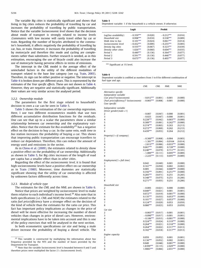
Table 5Dependent variable: 1 if the household is a vehicle owner, 0 otherwise.

Logit Probit

Log(bus availability) �0.359nnn (0.028) �0.212nnn (0.016)

Household size 0.998nnn (0.018) 0.538nnn (0.009)

Walk time to bus 0.101nnn (0.024) 0.061nnn (0.014)

Socioeconomic level �0.432nnn (0.009) �0.255nnn (0.005)

Density big cities 0.555nnn (0.067) 0.323nnn (0.039)

Density other cities 1.026nnn (0.060) 0.604nnn (0.035)

Period 1 0.449nnn (0.136) 0.364nnn (0.077)

Period 2 0.591nnn (0.136) 0.446nnn (0.077)

Period 3 0.675nnn (0.136) 0.495nnn (0.077)

nnn Significant at 1% level.

Table 6Dependent variable is codified as numbers from 1 to 8 for different combination of

fuel type and age.

CML CML NML NML

Alternative specific

Independent variable

(Car price)nsocioeconomic �0.012nnn (0.001) �0.001 (0.000)

(Fuel price/efficiency)n Socioeconomic �0.065nnn (0.008) �0.001 (0.000)

Case specific

Independent variable

Driver gender(male¼1)

2 �0.007 (0.047) �0.000 (0.001)

3 �0.025 (0.047) �0.000 (0.001)

4 0.228nnn (0.042) 0.003nnn (0.000)

5 0.309nnn (0.081) 0.262nnn (0.000)

6 0.374nnn (0.065) 0.263 (0.213)

7 0.272nnn (0.069) 0.262 (0.215)

8 0.439nnn (0.053) 0.264 (0.212)

Property(1¼ if company)

2 �0.360nnn (0.068) �0.004 (0.003)

3 �1.381nnn (0.084) �0.0164 (0.014)

4 �2.813nnn (0.086) �0.033nnn (0.000)

5 0.667nnn (0.089) 0.728nnn (0.000)

6 0.240nnn (0.079) 0.711nnn (0.101)

7 �1.089nnn (0.111) 0.695nnn (0.089)

8 �2.225nnn (0.113) 0.695nnn (0.089)

Employment(1¼ full time)

2 0.042 (0.049) 0.001 (0.000)

3 0.161nnn (0.050) 0.002 (0.002)

4 0.005 (0.044) 0.000nnn (0.000)

5 0.356nnn (0.091) 0.251nnn (0.000)

6 0.285nnn (0.071) 0.251 (0.285)

7 0.348nnn (0.075) 0.251 (0.286)

8 0.271nnn (0.055) 0.251 (0.286)

Household size

2 �0.005 (0.021) 0.000 (0.000)

3 0.049nn (0.021) 0.001 (0.001)

4 0.072nnn (0.019) 0.001nnn (0.000)

5 0.135nnn (0.033) 0.053nnn (0.000)

6 0.101nnn (0.027) 0.053nnn (0.000)

7 0.124nnn (0.029) 0.053 (0.059)

8 0.080nnn (0.023) 0.053 (0.059)

Car size

2 �0.065nnn (0.017) �0.001 (0.001)

3 �0.090nnn (0.017) �0.001 (0.001)

4 �0.106nnn (0.015) �0.001nnn (0.000)

5 0.324nnn (0.024) 0.319nnn (0.000)

6 0.264nnn (0.021) 0.318nnn (0.000)

7 0.264nnn (0.022) 0.317nnn (0.013)

8 0.182nnn (0.018) 0.317nnn (0.013)


The variable Big cities is statistically significant and shows thatliving in big cities reduces the probability of travelling by car andincreases the probability of travelling by public transportation.Notice that the variable Socioeconomic level shows that the decisionabout mode of transport is strongly related to income levels.Commuters with low income will rarely travel either by car ortrain. Regarding the number of bicycles attributed to the commu-ter’s household, it affects negatively the probability of travelling bycar, bus, or train. However, it increases the probability of travellingby motorcycle and therefore this mode and cycling are comple-ments rather than substitutes. Further research is needed, as in thisestimation, encouraging the use of bicycle could also increase theuse of motorcycle having perverse effects in terms of emissions.

The intercept in the CML model is the average effect of theunincluded factors in the utility of the different modalities oftransport related to the base line category (see e.g. Train, 2003).Therefore, its sign can be either positive or negative. The intercept inTable 4 is broken down per different years. This is represented by theestimates of the Year specific effects. These are not shown in Table 4.However, they are negative and statistically significant. Additionallytheir values are very similar across the analysed period.

3.2.2. Ownership module

The parameters for the first stage related to household’sdecision to own a car can be seen in Table 5.

Table 5 shows the estimation of the car ownership regression.Here, I use two different econometrics models that use twodifferent accumulative distribution functions for the residuals.One can see that up to a scalar the parameters show a similarrelationship between car ownership and the explanatory vari-ables. Notice that the estimate for Bus availability25 has a negativeeffect on the decision to buy a car. In the same vein, walk time to

bus station increases the probability of buying a car. This showsthat improving public transportation can encourage travellers toreduce car dependence. Therefore, this can reduce the amount ofenergy used and emissions in the sector.

As in Chiou et al. (2009), the estimates related to density showa positive effect on the probability of car ownership. Additionallyas shown in Table 5, for Big cities increases of the length of roadper capita has a smaller effect than in other cities.

Regarding the effect of the socioeconomic level, it is found thathigh socioeconomic levels have a positive effect on car ownershipas in Train (1980). Moreover, time dummies are statisticallysignificant showing that the utility of car ownership is affectedby unknown factors differently across time.

3.2.3. Module of vehicle type

The estimates for the CML and the NML are shown in Table 6.Notice that prices are weighted by socioeconomic level to make

them relative to each individual’s income level.26 Also note that inboth specifications (i.e. CML and NLM) the estimates related to theratio fuel price/efficiency have a stronger effect on the decision ofthe kind of vehicle than the estimates for the ratio car price. Thisfact has important policy implications as changes in the price ofdiesel will be more effective for increasing the number of dieselvehicles than changes in price of diesel cars. However, environ-mental implications have to be taken into account and this is oneof the policy exercises that will be analysed in the next section.

In both econometric specifications car size and being a maledriver increase the probability of buying a diesel vehicle. The

Engine capacity

2 0.059 (0.052) 0.001 (0.001)

3 0.136nnn (0.052) 0.002 (0.001)

4 0.049 (0.046) 0.001nnn (0.000)

5 1.8399nnn (0.115) 2.029nnn (0.000)

6 1.9083nnn (0.084) 2.031nnn (0.000)

25 This variable is constructed by multiplying the information about bus

frequency provided by the NTS and the number of buses provided by the

Department for Transport.26 Note that the variable Socioeconomic level is bounded between 0 and 5 and

therefore prices were multiplied the factor (1þSocioeconomic level).

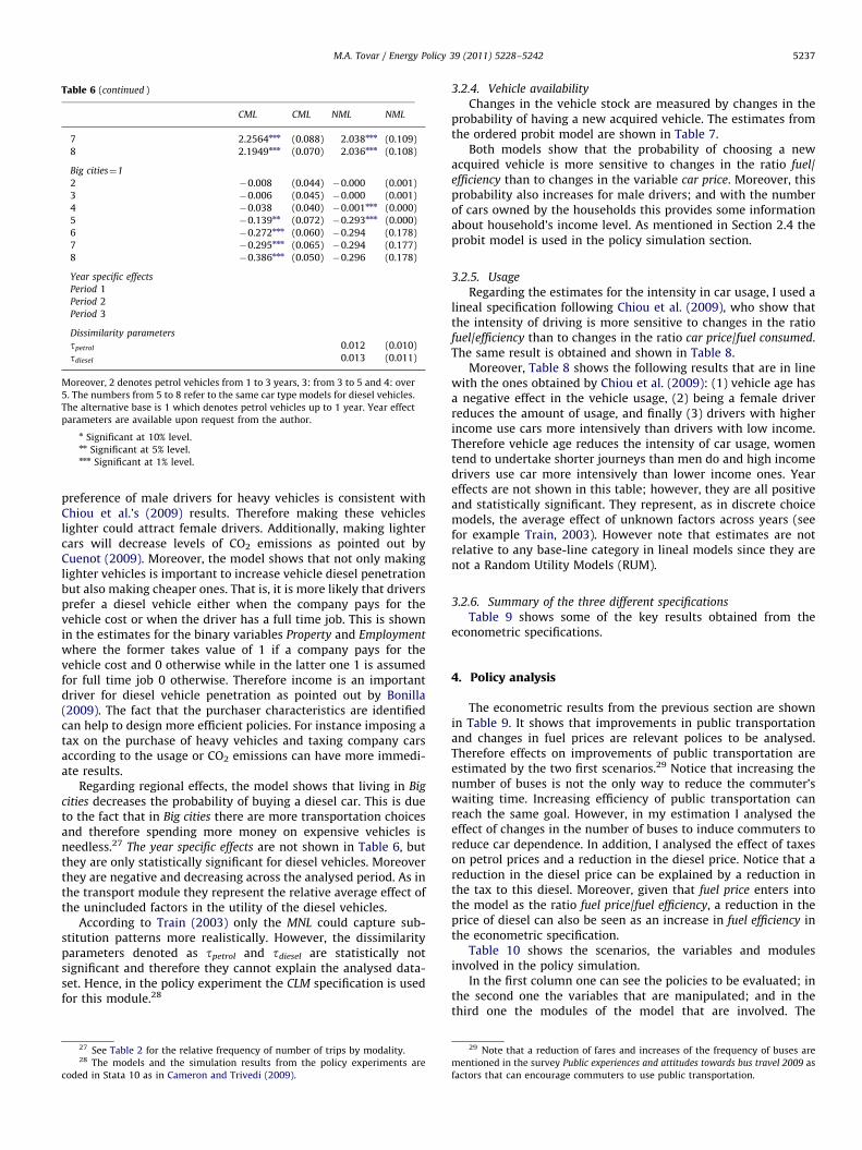
Table 6 (continued )

CML CML NML NML

7 2.2564nnn (0.088) 2.038nnn (0.109)

8 2.1949nnn (0.070) 2.036nnn (0.108)

Big cities¼1

2 �0.008 (0.044) �0.000 (0.001)

3 �0.006 (0.045) �0.000 (0.001)

4 �0.038 (0.040) �0.001nnn (0.000)

5 �0.139nn (0.072) �0.293nnn (0.000)

6 �0.272nnn (0.060) �0.294 (0.178)

7 �0.295nnn (0.065) �0.294 (0.177)

8 �0.386nnn (0.050) �0.296 (0.178)

Year specific effects

Period 1

Period 2

Period 3

Dissimilarity parameters

tpetrol 0.012 (0.010)

tdiesel 0.013 (0.011)

Moreover, 2 denotes petrol vehicles from 1 to 3 years, 3: from 3 to 5 and 4: over

5. The numbers from 5 to 8 refer to the same car type models for diesel vehicles.

The alternative base is 1 which denotes petrol vehicles up to 1 year. Year effect

parameters are available upon request from the author.

n Significant at 10% level.nn Significant at 5% level.nnn Significant at 1% level.


preference of male drivers for heavy vehicles is consistent withChiou et al.’s (2009) results. Therefore making these vehicleslighter could attract female drivers. Additionally, making lightercars will decrease levels of CO2 emissions as pointed out byCuenot (2009). Moreover, the model shows that not only makinglighter vehicles is important to increase vehicle diesel penetrationbut also making cheaper ones. That is, it is more likely that driversprefer a diesel vehicle either when the company pays for thevehicle cost or when the driver has a full time job. This is shownin the estimates for the binary variables Property and Employment

where the former takes value of 1 if a company pays for thevehicle cost and 0 otherwise while in the latter one 1 is assumedfor full time job 0 otherwise. Therefore income is an importantdriver for diesel vehicle penetration as pointed out by Bonilla(2009). The fact that the purchaser characteristics are identifiedcan help to design more efficient policies. For instance imposing atax on the purchase of heavy vehicles and taxing company carsaccording to the usage or CO2 emissions can have more immedi-ate results.

Regarding regional effects, the model shows that living in Big

cities decreases the probability of buying a diesel car. This is dueto the fact that in Big cities there are more transportation choicesand therefore spending more money on expensive vehicles isneedless.27 The year specific effects are not shown in Table 6, butthey are only statistically significant for diesel vehicles. Moreoverthey are negative and decreasing across the analysed period. As inthe transport module they represent the relative average effect ofthe unincluded factors in the utility of the diesel vehicles.

According to Train (2003) only the MNL could capture sub-stitution patterns more realistically. However, the dissimilarityparameters denoted as tpetrol and tdiesel are statistically notsignificant and therefore they cannot explain the analysed data-set. Hence, in the policy experiment the CLM specification is usedfor this module.28

27 See Table 2 for the relative frequency of number of trips by modality.28 The models and the simulation results from the policy experiments are

coded in Stata 10 as in Cameron and Trivedi (2009).

3.2.4. Vehicle availability

Changes in the vehicle stock are measured by changes in theprobability of having a new acquired vehicle. The estimates fromthe ordered probit model are shown in Table 7.

Both models show that the probability of choosing a newacquired vehicle is more sensitive to changes in the ratio fuel/efficiency than to changes in the variable car price. Moreover, thisprobability also increases for male drivers; and with the numberof cars owned by the households this provides some informationabout household’s income level. As mentioned in Section 2.4 theprobit model is used in the policy simulation section.

3.2.5. Usage

Regarding the estimates for the intensity in car usage, I used alineal specification following Chiou et al. (2009), who show thatthe intensity of driving is more sensitive to changes in the ratiofuel/efficiency than to changes in the ratio car price/fuel consumed.The same result is obtained and shown in Table 8.

Moreover, Table 8 shows the following results that are in linewith the ones obtained by Chiou et al. (2009): (1) vehicle age hasa negative effect in the vehicle usage, (2) being a female driverreduces the amount of usage, and finally (3) drivers with higherincome use cars more intensively than drivers with low income.Therefore vehicle age reduces the intensity of car usage, womentend to undertake shorter journeys than men do and high incomedrivers use car more intensively than lower income ones. Yeareffects are not shown in this table; however, they are all positiveand statistically significant. They represent, as in discrete choicemodels, the average effect of unknown factors across years (seefor example Train, 2003). However note that estimates are notrelative to any base-line category in lineal models since they arenot a Random Utility Models (RUM).

3.2.6. Summary of the three different specifications

Table 9 shows some of the key results obtained from theeconometric specifications.

4. Policy analysis

The econometric results from the previous section are shownin Table 9. It shows that improvements in public transportationand changes in fuel prices are relevant polices to be analysed.Therefore effects on improvements of public transportation areestimated by the two first scenarios.29 Notice that increasing thenumber of buses is not the only way to reduce the commuter’swaiting time. Increasing efficiency of public transportation canreach the same goal. However, in my estimation I analysed theeffect of changes in the number of buses to induce commuters toreduce car dependence. In addition, I analysed the effect of taxeson petrol prices and a reduction in the diesel price. Notice that areduction in the diesel price can be explained by a reduction inthe tax to this diesel. Moreover, given that fuel price enters intothe model as the ratio fuel price/fuel efficiency, a reduction in theprice of diesel can also be seen as an increase in fuel efficiency inthe econometric specification.

Table 10 shows the scenarios, the variables and modulesinvolved in the policy simulation.

In the first column one can see the policies to be evaluated; inthe second one the variables that are manipulated; and in thethird one the modules of the model that are involved. The

29 Note that a reduction of fares and increases of the frequency of buses are

mentioned in the survey Public experiences and attitudes towards bus travel 2009 as

factors that can encourage commuters to use public transportation.

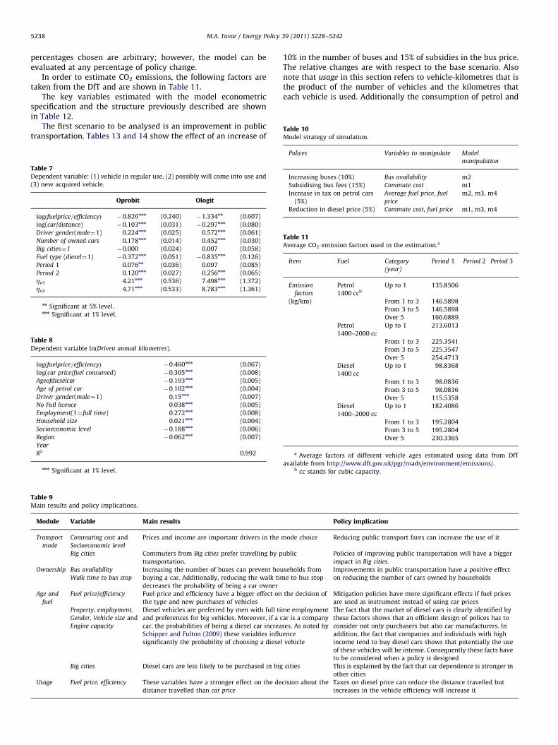
Table 10Model strategy of simulation.


percentages chosen are arbitrary; however, the model can beevaluated at any percentage of policy change.

In order to estimate CO2 emissions, the following factors aretaken from the DfT and are shown in Table 11.

The key variables estimated with the model econometricspecification and the structure previously described are shownin Table 12.

The first scenario to be analysed is an improvement in publictransportation. Tables 13 and 14 show the effect of an increase of

Table 7Dependent variable: (1) vehicle in regular use, (2) possibly will come into use and

(3) new acquired vehicle.

Oprobit Ologit

logðfuelprice=efficiencyÞ �0.826nnn (0.240) �1.334nn (0.607)

log(car/distance) �0.103nnn (0.031) �0.297nnn (0.080)

Driver gender(male¼1) 0.224nnn (0.025) 0.572nnn (0.061)

Number of owned cars 0.178nnn (0.014) 0.452nnn (0.030)

Big cities¼1 �0.000 (0.024) 0.007 (0.058)

Fuel type (diesel¼1) �0.372nnn (0.051) �0.835nnn (0.126)

Period 1 0.076nn (0.036) 0.097 (0.085)

Period 2 0.120nnn (0.027) 0.256nnn (0.065)

Za1 4.21nnn (0.536) 7.498nnn (1.372)

Za2 4.71nnn (0.533) 8.783nnn (1.361)

nn Significant at 5% level.nnn Significant at 1% level.

Table 8

Dependent variable lnðDriven annual kilometres).

logðfuelprice=efficiencyÞ �0.460nnn (0.067)

log(car price/fuel consumed) �0.305nnn (0.008)

Ageofdieselcar �0.193nnn (0.005)

Age of petrol car �0.102nnn (0.004)

Driver gender(male¼1) 0.15nnn (0.007)

No Full licence 0.038nnn (0.005)

Employment(1¼ full time) 0.272nnn (0.008)

Household size 0.021nnn (0.004)

Socioeconomic level �0.188nnn (0.006)

Region �0.062nnn (0.007)

Year

R2 0.992

nnn Significant at 1% level.

Table 9Main results and policy implications.

Module Variable Main results

Transport

mode

Commuting cost and

Socioeconomic level

Prices and income are important drivers in the

Big cities Commuters from Big cities prefer travelling by p

transportation.

Ownership Bus availability Increasing the number of buses can prevent hou

buying a car. Additionally, reducing the walk tim

decreases the probability of being a car owner

Walk time to bus stop

Age and

fuel

Fuel price/efficiency Fuel price and efficiency have a bigger effect on

the type and new purchases of vehicles

Property, employment,

Gender, Vehicle size and

Engine capacity

Diesel vehicles are preferred by men with full ti

and preferences for big vehicles. Moreover, if a c

car, the probabilities of being a diesel car increa

Schipper and Fulton (2009) these variables influ

significantly the probability of choosing a diesel

Big cities Diesel cars are less likely to be purchased in big

Usage Fuel price, efficiency These variables have a stronger effect on the de

distance travelled than car price

10% in the number of buses and 15% of subsidies in the bus price.The relative changes are with respect to the base scenario. Alsonote that usage in this section refers to vehicle-kilometres that isthe product of the number of vehicles and the kilometres thateach vehicle is used. Additionally the consumption of petrol and

Policy implication

mode choice Reducing public transport fares can increase the use of it

ublic Policies of improving public transportation will have a bigger

impact in Big cities.

seholds from

e to bus stop

Improvements in public transportation have a positive effect

on reducing the number of cars owned by households

the decision of Mitigation policies have more significant effects if fuel prices

are used as instrument instead of using car prices

me employment

ar is a company

ses. As noted by

ence

vehicle

The fact that the market of diesel cars is clearly identified by

these factors shows that an efficient design of polices has to

consider not only purchasers but also car manufacturers. In

addition, the fact that companies and individuals with high

income tend to buy diesel cars shows that potentially the use

of these vehicles will be intense. Consequently these facts have

to be considered when a policy is designed

cities This is explained by the fact that car dependence is stronger in

other cities

cision about the Taxes on diesel price can reduce the distance travelled but

increases in the vehicle efficiency will increase it

Polices Variables to manipulate Model

manipulation

Increasing buses (10%) Bus availability m2

Subsidising bus fees (15%) Commute cost m1

Increase in tax on petrol cars

(5%)

Average fuel price, fuel

price

m2, m3, m4

Reduction in diesel price (5%) Commute cost, fuel price m1, m3, m4

Table 11Average CO2 emission factors used in the estimation.a

Item Fuel Category

(year)

Period 1 Period 2 Period 3

Emission

factors

Petrol

1400 ccb

Up to 1 135.8506

(kg/km) From 1 to 3 146.5898

From 3 to 5 146.5898

Over 5 166.6889

Petrol

1400–2000 cc

Up to 1 213.6013

From 1 to 3 225.3541

From 3 to 5 225.3547

Over 5 254.4713

Diesel

1400 cc

Up to 1 98.8368

From 1 to 3 98.0836

From 3 to 5 98.0836

Over 5 115.5358

Diesel

1400–2000 cc

Up to 1 182.4086

From 1 to 3 195.2804

From 3 to 5 195.2804

Over 5 230.3365

a Average factors of different vehicle ages estimated using data from DfT

available from http://www.dft.gov.uk/pgr/roads/environment/emissions/.b cc stands for cubic capacity.


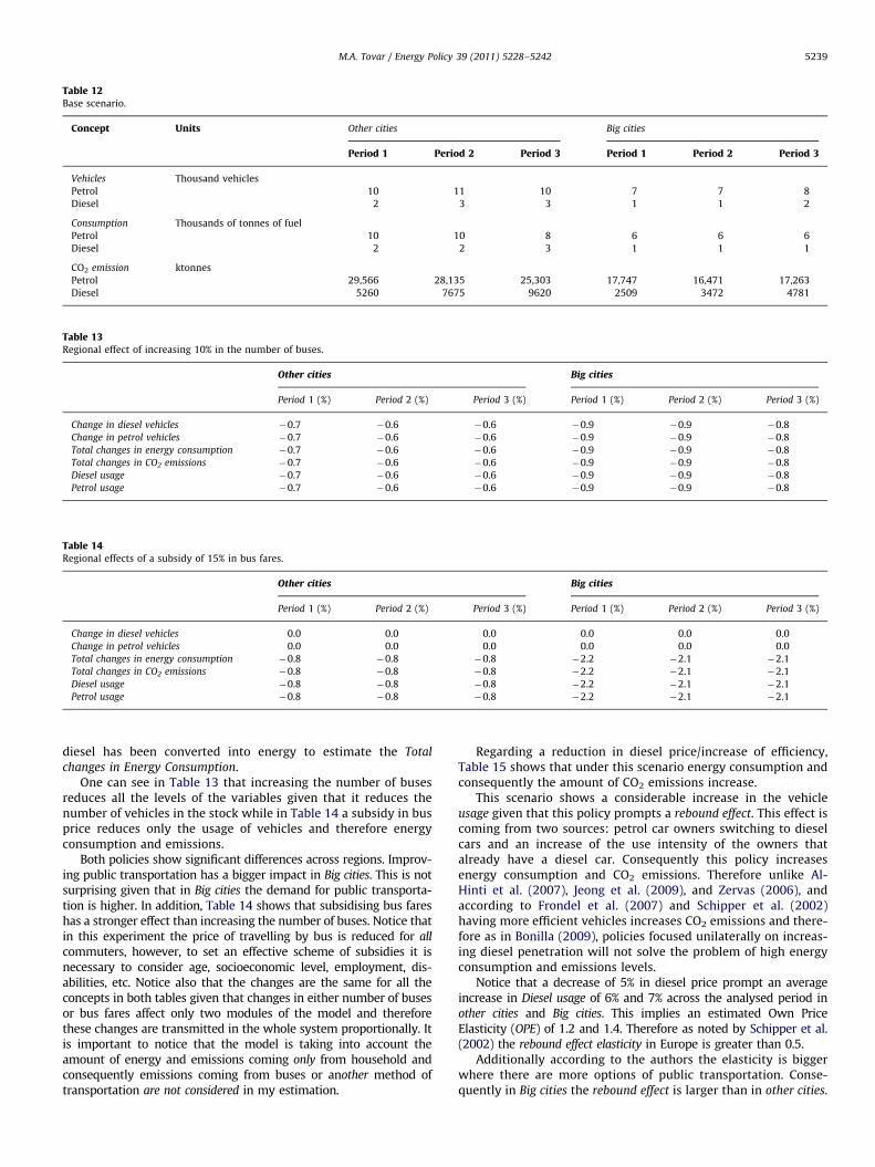
Table 12Base scenario.

Concept Units Other cities Big cities

Period 1 Period 2 Period 3 Period 1 Period 2 Period 3

Vehicles Thousand vehicles

Petrol 10 11 10 7 7 8

Diesel 2 3 3 1 1 2

Consumption Thousands of tonnes of fuel

Petrol 10 10 8 6 6 6

Diesel 2 2 3 1 1 1

CO2 emission ktonnes

Petrol 29,566 28,135 25,303 17,747 16,471 17,263

Diesel 5260 7675 9620 2509 3472 4781

Table 13Regional effect of increasing 10% in the number of buses.

Other cities Big cities

Period 1 (%) Period 2 (%) Period 3 (%) Period 1 (%) Period 2 (%) Period 3 (%)

Change in diesel vehicles �0.7 �0.6 �0.6 �0.9 �0.9 �0.8

Change in petrol vehicles �0.7 �0.6 �0.6 �0.9 �0.9 �0.8

Total changes in energy consumption �0.7 �0.6 �0.6 �0.9 �0.9 �0.8

Total changes in CO2 emissions �0.7 �0.6 �0.6 �0.9 �0.9 �0.8

Diesel usage �0.7 �0.6 �0.6 �0.9 �0.9 �0.8

Petrol usage �0.7 �0.6 �0.6 �0.9 �0.9 �0.8

Table 14Regional effects of a subsidy of 15% in bus fares.



Change in diesel vehicles 0.0 0.0 0.0 0.0 0.0 0.0

Change in petrol vehicles 0.0 0.0 0.0 0.0 0.0 0.0



Diesel usage �0.8 �0.8 �0.8 �2.2 �2.1 �2.1

Petrol usage �0.8 �0.8 �0.8 �2.2 �2.1 �2.1


diesel has been converted into energy to estimate the Total

changes in Energy Consumption.One can see in Table 13 that increasing the number of buses

reduces all the levels of the variables given that it reduces thenumber of vehicles in the stock while in Table 14 a subsidy in busprice reduces only the usage of vehicles and therefore energyconsumption and emissions.

Both policies show significant differences across regions. Improv-ing public transportation has a bigger impact in Big cities. This is notsurprising given that in Big cities the demand for public transporta-tion is higher. In addition, Table 14 shows that subsidising bus fareshas a stronger effect than increasing the number of buses. Notice thatin this experiment the price of travelling by bus is reduced for all

commuters, however, to set an effective scheme of subsidies it isnecessary to consider age, socioeconomic level, employment, dis-abilities, etc. Notice also that the changes are the same for all theconcepts in both tables given that changes in either number of busesor bus fares affect only two modules of the model and thereforethese changes are transmitted in the whole system proportionally. Itis important to notice that the model is taking into account theamount of energy and emissions coming only from household andconsequently emissions coming from buses or another method oftransportation are not considered in my estimation.

Regarding a reduction in diesel price/increase of efficiency,Table 15 shows that under this scenario energy consumption andconsequently the amount of CO2 emissions increase.

This scenario shows a considerable increase in the vehicleusage given that this policy prompts a rebound effect. This effect iscoming from two sources: petrol car owners switching to dieselcars and an increase of the use intensity of the owners thatalready have a diesel car. Consequently this policy increasesenergy consumption and CO2 emissions. Therefore unlike Al-Hinti et al. (2007), Jeong et al. (2009), and Zervas (2006), andaccording to Frondel et al. (2007) and Schipper et al. (2002)having more efficient vehicles increases CO2 emissions and there-fore as in Bonilla (2009), policies focused unilaterally on increas-ing diesel penetration will not solve the problem of high energyconsumption and emissions levels.

Notice that a decrease of 5% in diesel price prompt an averageincrease in Diesel usage of 6% and 7% across the analysed period inother cities and Big cities. This implies an estimated Own PriceElasticity (OPE) of 1.2 and 1.4. Therefore as noted by Schipper et al.(2002) the rebound effect elasticity in Europe is greater than 0.5.

Additionally according to the authors the elasticity is biggerwhere there are more options of public transportation. Conse-quently in Big cities the rebound effect is larger than in other cities.

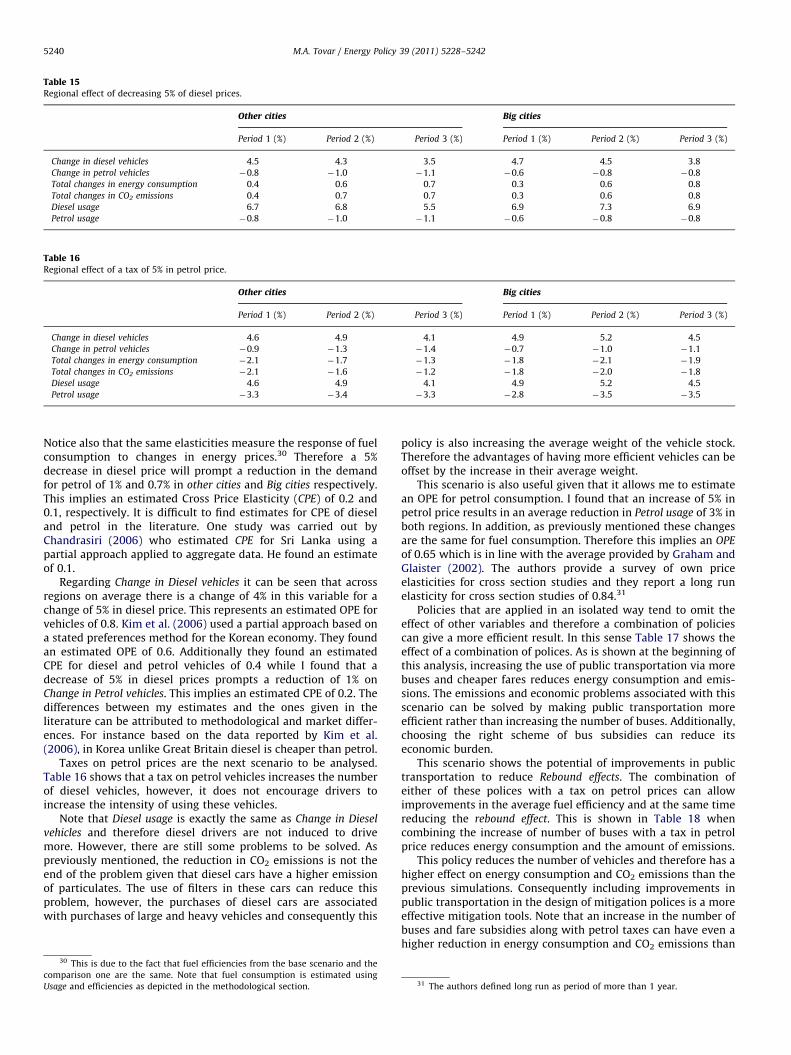
Table 15Regional effect of decreasing 5% of diesel prices.





Total changes in energy consumption 0.4 0.6 0.7 0.3 0.6 0.8

Total changes in CO2 emissions 0.4 0.7 0.7 0.3 0.6 0.8

Diesel usage 6.7 6.8 5.5 6.9 7.3 6.9

Petrol usage �0.8 �1.0 �1.1 �0.6 �0.8 �0.8

Table 16Regional effect of a tax of 5% in petrol price.







Diesel usage 4.6 4.9 4.1 4.9 5.2 4.5

Petrol usage �3.3 �3.4 �3.3 �2.8 �3.5 �3.5


Notice also that the same elasticities measure the response of fuelconsumption to changes in energy prices.30 Therefore a 5%decrease in diesel price will prompt a reduction in the demandfor petrol of 1% and 0.7% in other cities and Big cities respectively.This implies an estimated Cross Price Elasticity (CPE) of 0.2 and0.1, respectively. It is difficult to find estimates for CPE of dieseland petrol in the literature. One study was carried out byChandrasiri (2006) who estimated CPE for Sri Lanka using apartial approach applied to aggregate data. He found an estimateof 0.1.

Regarding Change in Diesel vehicles it can be seen that acrossregions on average there is a change of 4% in this variable for achange of 5% in diesel price. This represents an estimated OPE forvehicles of 0.8. Kim et al. (2006) used a partial approach based ona stated preferences method for the Korean economy. They foundan estimated OPE of 0.6. Additionally they found an estimatedCPE for diesel and petrol vehicles of 0.4 while I found that adecrease of 5% in diesel prices prompts a reduction of 1% onChange in Petrol vehicles. This implies an estimated CPE of 0.2. Thedifferences between my estimates and the ones given in theliterature can be attributed to methodological and market differ-ences. For instance based on the data reported by Kim et al.(2006), in Korea unlike Great Britain diesel is cheaper than petrol.

Taxes on petrol prices are the next scenario to be analysed.Table 16 shows that a tax on petrol vehicles increases the numberof diesel vehicles, however, it does not encourage drivers toincrease the intensity of using these vehicles.

Note that Diesel usage is exactly the same as Change in Diesel

vehicles and therefore diesel drivers are not induced to drivemore. However, there are still some problems to be solved. Aspreviously mentioned, the reduction in CO2 emissions is not theend of the problem given that diesel cars have a higher emissionof particulates. The use of filters in these cars can reduce thisproblem, however, the purchases of diesel cars are associatedwith purchases of large and heavy vehicles and consequently this

30 This is due to the fact that fuel efficiencies from the base scenario and the

comparison one are the same. Note that fuel consumption is estimated using

Usage and efficiencies as depicted in the methodological section.

policy is also increasing the average weight of the vehicle stock.Therefore the advantages of having more efficient vehicles can beoffset by the increase in their average weight.

This scenario is also useful given that it allows me to estimatean OPE for petrol consumption. I found that an increase of 5% inpetrol price results in an average reduction in Petrol usage of 3% inboth regions. In addition, as previously mentioned these changesare the same for fuel consumption. Therefore this implies an OPE

of 0.65 which is in line with the average provided by Graham andGlaister (2002). The authors provide a survey of own priceelasticities for cross section studies and they report a long runelasticity for cross section studies of 0.84.31

Policies that are applied in an isolated way tend to omit theeffect of other variables and therefore a combination of policiescan give a more efficient result. In this sense Table 17 shows theeffect of a combination of polices. As is shown at the beginning ofthis analysis, increasing the use of public transportation via morebuses and cheaper fares reduces energy consumption and emis-sions. The emissions and economic problems associated with thisscenario can be solved by making public transportation moreefficient rather than increasing the number of buses. Additionally,choosing the right scheme of bus subsidies can reduce itseconomic burden.

This scenario shows the potential of improvements in publictransportation to reduce Rebound effects. The combination ofeither of these polices with a tax on petrol prices can allowimprovements in the average fuel efficiency and at the same timereducing the rebound effect. This is shown in Table 18 whencombining the increase of number of buses with a tax in petrolprice reduces energy consumption and the amount of emissions.

This policy reduces the number of vehicles and therefore has ahigher effect on energy consumption and CO2 emissions than theprevious simulations. Consequently including improvements inpublic transportation in the design of mitigation polices is a moreeffective mitigation tools. Note that an increase in the number ofbuses and fare subsidies along with petrol taxes can have even ahigher reduction in energy consumption and CO2 emissions than

31 The authors defined long run as period of more than 1 year.

Table 17Regional effect of an increase of 10% in the number of buses and 15% of a subsidy in bus fares.



Change in diesel vehicles �0.7 �0.6 �0.6 �0.9 �0.9 �0.8




Diesel usage �1.5 �1.4 �1.4 �3.1 �3.0 �2.9

Petrol usage �1.5 �1.4 �1.4 �3.1 �3.0 �2.9

Table 18Regional effect of an increase of 10% in the number of buses and a 5% tax on petrol price.







Diesel usage 4.0 4.2 3.5 4.0 4.3 3.6

Petrol usage �3.9 �4.0 �3.9 �3.6 �4.3 �4.3


the ones shown in Table 18. However, these polices have to bereinforced to control possible rebound effects by the followingpolices: (1) Keeping higher diesel prices than petrol ones asfollowed in Great Britain can reduce rebound effects as thisdiscourages diesel drivers to increase the usage intensity, and(2) making mandatory the use of filters for diesel vehicles can alsoreduce the impact of the emission of particulates. Additionally, itis necessary to implement polices to prevent purchasers frombuying big vehicles as this is another source of the rebound effect.A possible mechanism can be similar to the French bonus32 whichaccording to Cuenot (2009) can reduce the amount of heavyvehicles and therefore the amount of CO2 emissions. It is impor-tant to notice that alternative policies addressed to reduce carusage needs to consider characteristics such as property, socio-

economic level and vehicle size as they proved in the mode to beimportant in the choice of vehicle and intensity of using thesevehicles.

5. Conclusions

In this paper, an integral approach was used to analyse theeffect of policies of increasing diesel vehicle penetration onenergy consumption and CO2 emissions. Using a survey carriedout in Great Britain, it was found that diesel vehicle penetrationfaces technical limitations that challenge the manufacture indus-try. The estimation shows the need to make lighter diesel carsthat have to be more accessible to all drivers regardless of genderor socioeconomic status. Moreover, the model provides empiricalevidence that policies aimed at having more efficient vehicles willincrease the intensity of using those cars. Consequently, thesepolicies increase energy consumption and CO2 emissions. Thisfinal conclusion is opposite to the one reached by Al-Hinti et al.(2007), Jeong et al. (2009), and Zervas (2006) who did not use anintegral approach. Therefore this paper provides empirical evi-dence that support Bonilla’s (2009) argument that the policy of

32 A subsidy designed by the French government to increase low CO2

emissions vehicles.

improving vehicle efficiency as part of the UK’s participation inthe European Union Voluntary agreement will not be able toachieve its goals of energy consumption and CO2 mitigation.Additionally, this result supports Frondel et al. (2007) andSchipper et al. (2002)’s argument that when energy servicesbecomes cheaper, it will prompt a rebound effect.

On the other hand, given that despite improvements in publictransportation there will be commuters who prefer to travel bycar, therefore, a better way to introduce more efficient vehicles inthe economy is by combining different policies. Therefore a tax onpetrol prices and improvements in public transportation is aneffective mitigation policy. However, this policy has to be rein-forced with other policies such as keeping a differential pricebetween petrol and diesel and introducing a mechanism like theFrench Bonus to reduce the number of heavy vehicles. An issue forfurther research is to include in the model a scrap module toestimate more accurate flows in vehicle stock and fuel consump-tion and CO2 emissions coming from motorcycles and buses.

References

Al-Hinti, I., Al-Ghandoor, A., Akash, B., Abu-Nada, E., 2007. Energy saving and CO2

mitigation through restructuring Jordan’s transportation sector: the dieselpassenger cars scenario. Energy Policy 35 (10), 5003–5011.

Azevedo, C.D., Herriges, J.A., Kling, C.L., 2003. Combining revealed and statedpreferences: consistency tests and their interpretations. American Journal ofAgricultural Economics 85 (3), 525–537.

Bonilla, D., 2009. Fuel demand on UK roads and dieselization of fuel economy.Energy Policy 37, 3769–3778.

Bonilla, D., Foxon, T., 2009. Demand for new car fuel economy in the UK, 1970–2005.Journal of Transport Economics and Policy 43 (Part 1), 55–83.

Ben-Akiva, M., 1974. Structure of passenger travel demand models. TransportationResearch Record 526, 26–42.

Ben-Akiva, M., Lerman, R.S., 1985. Discrete Choice Analysis: Theory and Applica-tion toTravel Demand. The MIT Press.

Cameron, C.A., Trivedi, P.K., 2005. Microeconometrics, Methods and Applications.Cambridge University Press, New York.

Cameron, C.A., Trivedi, P.K., 2009. Microeconomics Using Sata. Stata Press.Chandrasiri, 2006. Demand for road–fuel in a small developing economy: the case

of Sri Lanka. Energy Policy 34, 1833–1840.Chiou, Y.C., Wen, C.H., Tsai, S.H., Wang, W.Y., 2009. Integrated modeling of car/

motorcycle ownership, type and usage for estimating energy consumption andemissions. Transportation Research Part A: Policy and Practice 43 (7), 2009.


Cuenot, Francois, 2009. CO2 emissions from new cars and vehicle weight inEurope: how the EU regulation could have been avoided ah how to reach it?Energy Policy 37 (10), 3832–3842.

Dargay, J., Hanly, M., 2004a. Land Use and Mobility. ESRC Transport Studies Unit.Dargay, J., Hanly, M., 2004b. Volatility of Car Ownership, Commuting Mode and

Time in the UK. ESRC Transport Studies Unit.Frondel, M., Peters, J., Vance, C., 2007. Identifying the rebound: evidence from

Germany household panel. Rurh Economic Paper.Frondel, M., Vance, C., 2010. Driving for fun? Comparing the effect of fuel prices on

weekday and weekend fuel consumption. Energy Economics 32, 102–109.Graham, D.J., Glaister, S., 2002. The demand for automobile fuel: a survey of

elasticities. Journal of Transport Economics and Policy 36 (1), 1–25.Heckman, J.J., 1979. Sample selection bias as a specification error. Econometrica 47

(1), 153–161.Hole, A., FitzRoy, F., 2004. Commuting in Small Towns in Rural Areas: The Case of

St. Andrews. Department of Economics, University of St. Andrews.Jeong, S.J., Kim, K.S., Park, J.W., 2009. CO2 emissions change from the sales authoriza-

tion of diesel passenger cars: Korean case study. Energy Policy 37 (7), 2630–2638.Kim, J.H., Lee, S., Preston, J., 2006. The impact of the fuel price policy on the

demand for diesel passenger cars in Korean cities. International Review ofPublic Administration 10 (2), 61–73.

Lee, J., Cho, Y., 2009. Demand forecasting of diesel passenger car consideringconsumer preference and government regulation in South Korea. Transporta-tion Research Part A: Policy and Practice 43 (4), 420–429.

Mohammadian, A., Miller, E.J., 2003. Empirical investigation of household vehicletype choice decisions. Transportation Research Record 1854, 99–106.

Schipper, L., Marie-Lilliu, C., Fulton, L., 2002. Diesel in Europe: Analysis ofcharacteristics, usage patterns, energy savings and CO2 emissions implica-tions. Journal of Transport Economics and Policy 36 (Part 2), 305–340.

Schipper, L., 2009. Carbon in motion: Fuel economy, vehicle use and other factorsaffecting CO2 emissions from transport (editorial). Energy Policy 37 (10),3711–3713.

Schipper, L., Fulton, L., 2009. Disappointed by diesel? Impact of shift to diesels inEurope through 2006. Transport Research Board 2139, 1–10.

Train, K., 1980. A structured logit model of auto ownership and mode choice.Review of Economic Studies 47, 357–370.

Train, K., 2003. Discrete Choice Methods with Simulation. Cambridge University Press.Vaage, Kjell, 2000. Heating technology and energy use: a discrete/continuous

choice approach to Norwegian household energy demand. Energy Economics22, 649–666.

Zervas, E., 2006. CO2 benefit from the increasing percentage of diesel passengercars. Case of Ireland. Energy Policy 34 (17), 2848–2857.

Documents

An integral evaluation of dieselisation policies for households’ cars