An integrated analysis of lidar observations in association with optical properties of aerosols from a high altitude location in central Himalayas

ATMOSPHERIC SCIENCE LETTERSAtmos. Sci. Let. 10: 48–57 (2009)Published online 23 January 2009 in Wiley InterScience(www.interscience.wiley.com) DOI: 10.1002/asl.209

An integrated analysis of lidar observations in associationwith optical properties of aerosols from a high altitudelocation in central Himalayas

P. Hegde,1†* P. Pant1 and Y. Bhavani Kumar2

1Aryabhatta Research Institute of Observational Sciences (ARIES), Nainital, India2National Atmospheric Research Laboratory (NARL), Gadanki, India

*Correspondence to:P. Hegde, Aryabhatta ResearchInstitute of ObservationalSciences (ARIES), Nainital, India.E-mail:[email protected]

†Current address: Space PhysicsLaboratory (SPL), VikramSarabhai Space Centre (VSSC),Indian Space ResearchOrganization,Trivandrum-695022 Kerala,India.

Received: 4 April 2008Revised: 21 November 2008Accepted: 3 December 2008

AbstractIn order to study the aerosol backscatter profiles, a portable micro pulse lidar (MPL) systemwas installed in the year 2006 at Manora Peak, (29◦22′N, 79◦27′E, ∼1960 m amsl) Nainital, ahigh altitude location in the central Himalayas. In the present study the results of observedlidar profiles, columnar aerosol optical depths (AOD) and prevailing meteorology duringMay 2006 to June 2007 are presented. Although the lidar was operated from a sparselyinhabited free tropospheric site, nevertheless the height distribution of aerosol layers arefound to be extended up to the summit of ∼2 km above the ground level (AGL). Thebackscatter ratio (BSR) varies from ∼10 to ∼20 having lowest values during post-monsoonand highest during pre-monsoon period. The observed boundary layer height during the postmonsoon was shallower to the pre-monsoon period. Occasionally the lidar profiles reveal thepresence of cirrus clouds at an altitude of 8–10 km AGL. The extended lidar observationsover Manora Peak not only provided the profiles of aerosol extinction coefficient but alsosignificantly substantiate the elevated aerosol layers and clouds, which are important in thestudy of climate modelling. Copyright 2009 Royal Meteorological Society

Keywords: lidar profiles; atmospheric aerosols; backscatter ratio; cirrus clouds

1. Introduction

Atmospheric aerosols have a direct effect on the radia-tive forcing in the atmosphere as they scatter andabsorb solar and infrared radiation in the atmosphere(Charlson et al., 1992) and indirectly affect the sizedistribution of cloud droplets (IPCC, 2007). It isan established fact that aerosols significantly affectthe earth radiation budget through the scattering andabsorption of incoming solar radiation. In this perspec-tive the temporal and spatial distributions of aerosolin the lower atmosphere are important in assessingtheir impact on the earth’s climate. In addition tothese effects, aerosols also play an important rolein providing the information on the development ofcloud microphysics, climate variability, atmosphericpollution and atmospheric boundary layer evaluation(Lagrosas et al., 2004). Lidar has so far shown thebest performance in defining the position of aerosoland clouds with high temporal and spatial resolu-tion, which is not possible with other kind of remotesensing techniques (Devara et al., 1995; Raj et al.,1996). Lidar can provide vertically resolved extinc-tion and backscatter coefficients, and thereby provid-ing the height of the planetary boundary layer or thenight-time residual layer. A thorough knowledge ofoptical properties of atmospheric aerosol such as theextinction and optical depth as well as their temporal

and vertical distribution are essential for understandingtheir effects on the atmosphere.

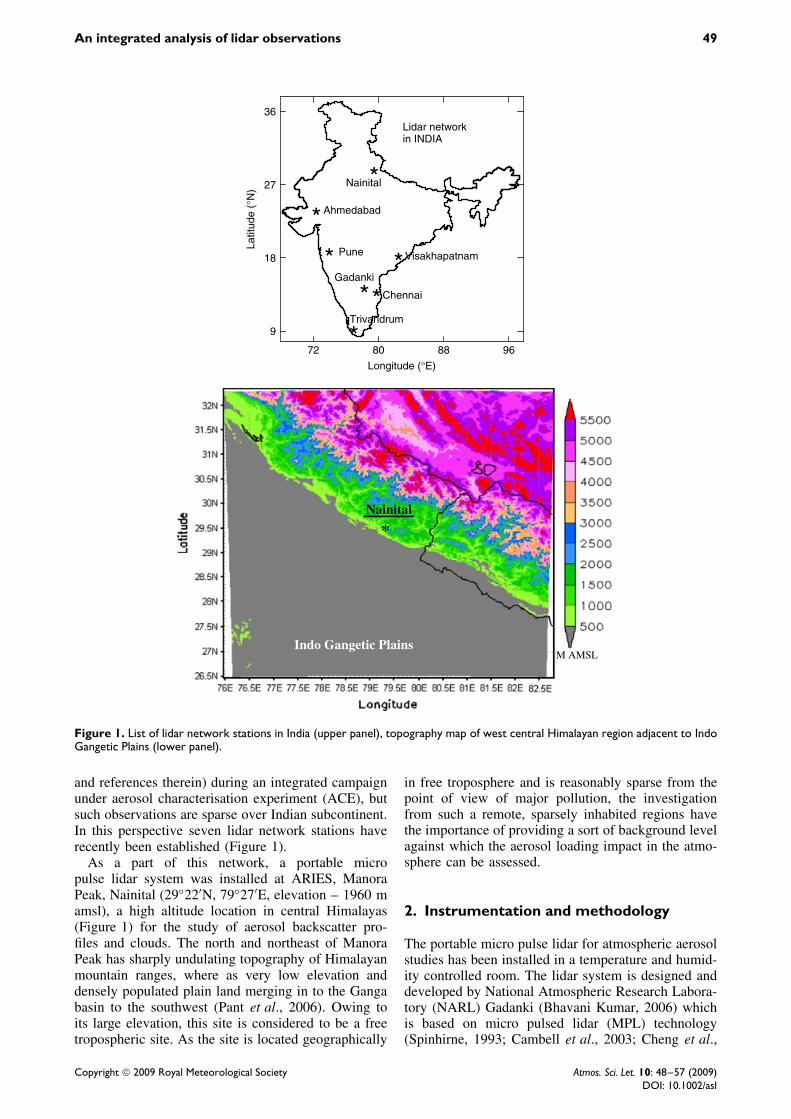
Lidar has also proven to be a powerful means tostudy cloud characteristics particularly of cirrus cloudswith high range and time resolution. These cloudsare usually found at an altitude, ranging from 8 to20 km Devara et al., 1995; and often extend to morethan 1000 km horizontally and persist for up to sev-eral days (Immler and Schrems, 2002). These cloudsare produced by the outflow of deep convection cloudanvils of the slow synoptic scale uplifting of a moistair layer and homogeneous nucleation (Thomas et al.,2002). Although the role of the tropical cirrus cloudsin the overall global climate system is not completelyunderstood however they dominate the cloud radia-tive forcing especially over the tropics (Sunil Kumaret al., 2003). Parameswaran et al. (1991) compared theaerosol extinction profiles derived from Sage II satel-lite data with lidar observations over tropical coastalstation, Trivandrum (Figure 1). They found large dayto day as well as latitudinal and longitudinal changesin tropospheric extinction, which points out the impor-tance of the study of tropospheric aerosol extinctionat different locations even within the tropical regionfor understanding of the behaviour of troposphericaerosols.

Over the years, several ground and space basedlidar observations were simultaneously conducted overthe East Asian region (e.g. Murayama et al., 2003,

Copyright 2009 Royal Meteorological Society

An integrated analysis of lidar observations 49

Longitude (°E)

72 80 88 96

Latit

ude

(°N

)

9

18

27

36

Nainital

Lidar networkin INDIA

Ahmedabad

Visakhapatnam

Chennai

Pune

Gadanki

Trivandrum

Indo Gangetic Plains

Nainital

M AMSL

Figure 1. List of lidar network stations in India (upper panel), topography map of west central Himalayan region adjacent to IndoGangetic Plains (lower panel).

and references therein) during an integrated campaignunder aerosol characterisation experiment (ACE), butsuch observations are sparse over Indian subcontinent.In this perspective seven lidar network stations haverecently been established (Figure 1).

As a part of this network, a portable micropulse lidar system was installed at ARIES, ManoraPeak, Nainital (29◦22′N, 79◦27′E, elevation – 1960 mamsl), a high altitude location in central Himalayas(Figure 1) for the study of aerosol backscatter pro-files and clouds. The north and northeast of ManoraPeak has sharply undulating topography of Himalayanmountain ranges, where as very low elevation anddensely populated plain land merging in to the Gangabasin to the southwest (Pant et al., 2006). Owing toits large elevation, this site is considered to be a freetropospheric site. As the site is located geographically

in free troposphere and is reasonably sparse from thepoint of view of major pollution, the investigationfrom such a remote, sparsely inhabited regions havethe importance of providing a sort of background levelagainst which the aerosol loading impact in the atmo-sphere can be assessed.

2. Instrumentation and methodology

The portable micro pulse lidar for atmospheric aerosolstudies has been installed in a temperature and humid-ity controlled room. The lidar system is designed anddeveloped by National Atmospheric Research Labora-tory (NARL) Gadanki (Bhavani Kumar, 2006) whichis based on micro pulsed lidar (MPL) technology(Spinhirne, 1993; Cambell et al., 2003; Cheng et al.,

Copyright 2009 Royal Meteorological Society Atmos. Sci. Let. 10: 48–57 (2009)DOI: 10.1002/asl

50 P. Hegde, P. Pant and Y. Bhavani Kumar

2005). Lidar observations are carried out at Nainitalon regular basis to study the aerosol vertical pro-file, the boundary layer structures, cloud base heightand its vertical extent. The system employs a diodepumped Nd : YAG laser with second harmonic out-put at 532 nm and operated at 2500 Hz. The emit-ter beam is coaxial to receiver field of view (FOV)and operated in zenith direction. The lidar receiveremploys a 150-mm cassegrainin telescope and a highgain photo multiplier tube (PMT) operating in pho-ton counting mode. The complete overlap betweenthe laser beam and the telescope FOV is expected at∼150 m. This value represents the lower limit of ourvertical lidar profiles. The backscattered signals aremeasured with a bin width of 200 ns correspondingto the altitude range of 30 m. Computer based multi-channel analyser (MCA) was employed for recordingthe photon returns. During the observations the lidarsystem collects the backscattered signal returns fromthe lower atmospheric aerosol and high altitude cloudsuch as cirrus. The data were processed using algo-rithm described by Fernald (1984) and Klett (1985)for deriving the aerosol extinction coefficient profilesand other related atmospheric parameters. The inver-sion lidar profiles are based on the solution of the lidarequation for the case of single scattering (Measures,1984), given as:

P(λ, R) = PLAOξ(λ)

R2 β(λ, R)ζ(R)cτ1

2

exp[−2

∫ R

0α(λ, R)dR

](1)

where, P(λ, R) is the lidar signal received from arange R at a wavelength λ, PL is the emitted laserpower, Ao is the telescope receiving area, ξ(λ) is thereceivers spectral transmission factor, β(λ,R) is theatmospheric volume backscattering coefficient, ζ (R) isthe overlap factor between the FOV of the telescopeand the laser beam, α(λ,R) is the extinction coeffi-cient from atmospheric molecules and particles, c isthe speed of light and τl is the laser pulse length.The lidar data have been processed with the algo-rithm described by (Fernald, 1984; Klett, 1985), wherethe molecular (or Rayleigh) contribution to the sig-nal is taken from the COSPAR International Refer-ence Atmosphere (CIRA) 1986 standard atmosphere.According to the Fernald–Klett formulation, the solu-tion of the lidar equation is given as:

β(R) = exp{−[S ′(Rref) − S ′(R)]}1

β(Rref)+ 2

C∫ Rref

R dR′

exp{−[S ′(Rref) − S ′(R′)]}

(2)

where, the total backscattering coefficient is the sum ofRayleigh and particulate contribution given by β(R) =βp(R) + βR(R), the β(Rref) is the boundary condition

set on β(R) at the reference far-end range. The solu-tion to the above equation is given numerically asunder:

S ′(Rref) − S ′(R) = ln[R2ref × P(Rref)]

− ln[R2 × P(R)] − 3

4π

∫ Rref

RβR(R′)dR′

+ 2

C

∫ Rref

RβR(R′)dR′ (3)

The above equations were derived by taking thevalue of C equal to 0.035, an average value for rural,urban and maritime aerosols (Kovalev, 1993), the ref-erence range (Rref) in a region where the lidar profilefollows the molecular atmosphere (generally between4 and 6 km) and assuming that the backscatter-to-extinction ratio is known. Besides the lidar obser-vations the measurements of aerosol optical depthusing the Microtops II, Sun Photometer (Solar LightCo., USA) and meteorological parameters using, stan-dard meteorological sensors (Campbell Scientific Inc.,Canada) attached with automatic weather stations,were also carried out.

3. Results and discussion

3.1. Surface meteorology

The monthly mean variations of surface meteoro-logical parameters for temperature, columnar watervapour, rainfall, wind speed and wind direction atManora Peak are provided in Table I. Monthly meantemperature varies from its maximum value of 28.5 ◦Cduring May and shows gradual decreasing trend duringrainy season and minimum temperatures occur dur-ing January and February. The columnar water vapourcontent remains less than 1 cm in 80% of the measure-ments, with a mean value of 0.64 cm implying a dryenvironment. Humidity is particularly high with thearrival of monsoon from mid June to end of Septem-ber. The rainfall climatology shows that the rainfall ishighest during July to September owing to the south-west monsoon over the Indian subcontinent (account-ing ∼70% of the annual rainfall), with very little rainduring March to middle of June (∼10% of the annual).The wind speed, during post-monsoon (September,October and November) and winter months (Decem-ber, January and February) remains ∼10 m s−1 butduring pre-monsoon (March, April and May) as well asduring the monsoon (June, July and August) it is maxi-mum and sometimes reaches up to ∼24 m s−1. Duringthe transition period from pre-monsoon to monsoonthe mean arrival wind direction gradually shifts fromsouthwesterly to southeasterly.

3.2. Overview of BSR characteristics

For the present study the lidar measurements are anal-ysed for the period of May 2006 to June 2007. The



Tab

leI.

Lida

rob

serv

atio

nde

tails

alon

gw

ithsu

rfac

em

eteo

rolo

gyan

dot

her

para

met

ers

(bri

efde

scri

ptio

nof

para

met

ers

are

incl

uded

)

Par

amet

ers

May

Jun

Jul

Aug

Sep

Oct

No

vD

ecJa

nF

ebM

arA

prM

ayJu

n

2006

2007

Profi

les

295

(3)

627

(6)

——

279

(4)

2098

(13)

1254

(15)

637

(6)

793

(9)

593

(3)

1041

(8)

887

(9)

602

(8)

42(2

)T m

ax28

.528

2625

2524

2321

2018

2225

28.5

28C

WV

0.55

0.77

1.83

1.39

1.28

0.63

0.51

0.26

0.24

0.32

0.51

0.48

0.56

0.81

Rain

fall

9012

047

755

425

332

1.3

122.

416

198

2929

835

1W

S23

2116

.411

.89.

39.

48.

58.

28.

812

1413

20.3

17W

D23

821

015

014

816

222

220

922

623

622

020

925

123

020

9Li

dar

AO

D0.

143

0.26

4—

—0.

071

0.04

40.

041

0.02

30.

034

0.04

20.

065

0.13

50.

176

0.14

7M

Tops

AO

D0.

210

0.31

40.

082

0.13

50.

090

0.06

20.

066

0.03

60.

050

0.07

60.

072

0.16

30.

228

0.31

7Tr

ajec

torie

s47

3826

1210

.513

106

24

1422

3438

Aer

osol

inde

x2.

971.

810.

680.

490.

610.

720.

49−0

.37

0.01

0.42

1.35

2.12

2.68

1.63

Profi

les,

tota

lnum

ber

oflid

arob

serv

atio

npr

ofile

sea

chha

ving

2m

indu

ratio

n,be

low

isth

enu

mbe

rin

pare

nthe

ses

give

tota

lnig

hts

for

whi

chob

serv

atio

nsw

ere

mad

e.T m

ax,m

axim

umte

mpe

ratu

re(◦

C).

CW

V,c

olum

nar

wat

erva

pour

cont

ent

(cm

)de

rived

from

Mic

roto

psII

sunp

hoto

met

er.

Rain

fall,

cum

ulat

ive

rain

fall

(mm

).W

S,av

erag

ew

ind

spee

d(m

/s).

WD

,win

ddi

rect

ion

(Deg

rees

).Li

dar

AO

D,l

idar

deriv

edae

roso

lopt

ical

dept

h(5

32nm

).M

Tops

AO

D,m

icro

tops

IIsu

npho

tom

eter

deriv

edae

roso

lopt

ical

dept

h(5

00nm

).Tr

ajec

torie

s,pe

rcen

tage

ofai

rm

ass

arriv

ing

from

sout

hwes

tdi

rect

ion.

Aer

osol

inde

x,To

talO

zone

Map

ping

Spec

trom

eter

(TO

MS)

/Ozo

neM

onito

ring

Inst

rum

ent

(OM

I)sa

tellit

eae

roso

lind

ex.



Monsoon(JJA months)

0 5 10 15 20

Hei

ght (

KM

)

1

2

3

4Postmonsoon(SON months)

0 5 10 15 20

1

2

3

4Winter(DJF months)

0 5 10 15 20

1

2

3

4Premonsoon(MAM months)

0 5 10 15 20

1

2

3

4

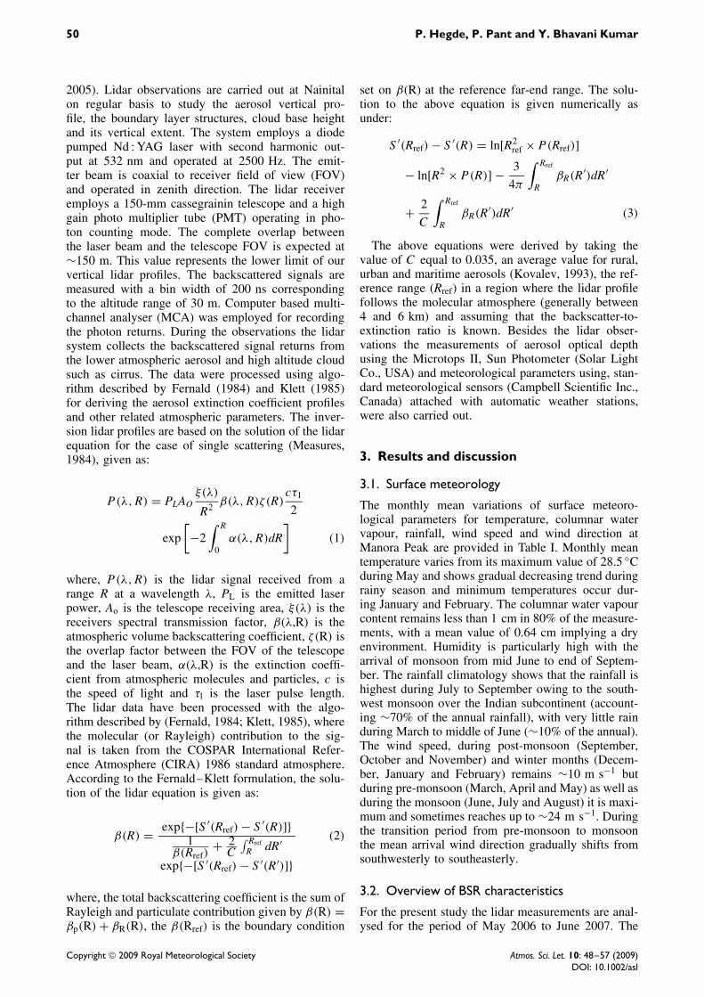
Figure 2. Vertical profiles of back scatter ratio (R) averaged for different seasons during May 2006 to June 2007. The horizontalbars represent the one standard deviation.

details of lidar observations along with other parame-ters are listed in Table I. Generally observations weremade from 1900 Indian Standard Time (IST) to 2400IST, but on few occasions the data were recordedfor entire night (i.e. from 1900 IST to 0500 IST).Figure 2 shows the profiles of back scattered ratio(BSR), calculated from the selected profiles represent-ing different seasons. Higher values of BSR are foundfor the prevailing strong convection conditions dur-ing summer months (March, April and May (MAM);when the wind is predominantly from southwesterly.It is quite discernible from the figure that aerosollayer often reaches up to an altitude of ∼2.0 km.The lower value of BSR during post-monsoon sea-son [September, October, November (SON)] may bedue to rain scavenging of aerosol from the lower tro-posphere. During summer months (pre-monsoon) thevertical extent of aerosols in the troposphere is largeover northwestern part of India due to increase in tem-perature as well as dust transport from Thar Desertregion (Hegde et al., 2007). The higher values of BSRover study region are attributed to the strong convec-tive conditions during these months, when aerosol anddust particles are often lifted up to free troposphereover the Northwestern India (Prasad et al., 2007). Theexchange of air masses from the boundary layer into the free troposphere is aided by mountain rangesand may thus affect the spatial as well as temporaldistribution of aerosol properties (Nyeki et al., 2000).

3.3. Mixed layer depth determination

The atmospheric boundary layer can be divided in tothree different layers: the surface layer, the mixedlayer and the entrainment zone (Stull, 1997). Theatmospheric entrainment zone is considered as a thin,convoluted sub-layer that separates the air transportedupwards from the mixed layer and the air transportedfrom the free atmosphere aloft (Mok and Rudowicz,2004). In aerosol studies, the mixed layer character-istics are most important since the pollutants that areemitted in to the atmospheric boundary layer are sub-jected to gradual dispersion and mixed through theaction of turbulence in this region which ultimately

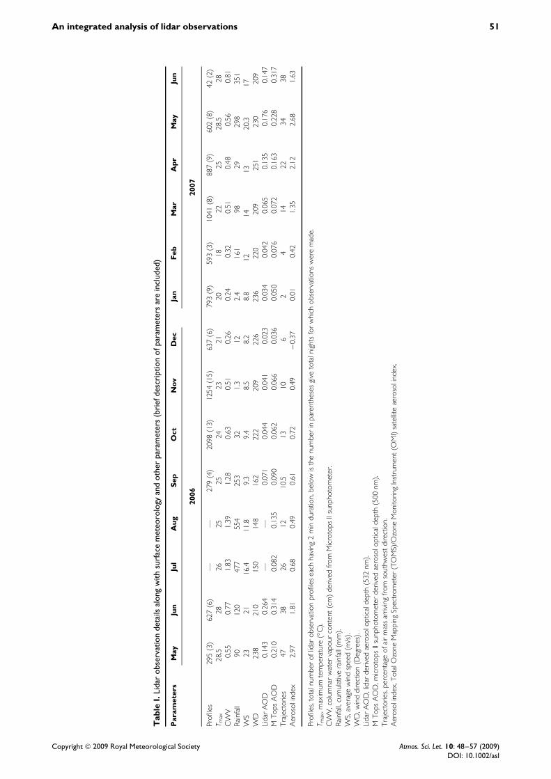
facilitate in modelling the vertical extent of the pol-lutant movement (Parameswaran et al., 1997; Menutet al., 1999). The maximum in the vertical gradientor the sharp upward decrease in the lidar backscatterreturn denotes the mixed layer depth, which should beobserved as the aerosols content in the mixed layercloser to the ground portion is higher than the airabove (Seibert et al., 1998). Eddies generated as aresult of surface heating are transported vertically upuntil the rising air parcel encounters a region havingequal ambient density. Therefore, the altitude regionwhere eddy transport is significant is referred to asthe well-mixed region (Parameswaran, 2001). The alti-tude profile in Figure 2 shows that the peak value ofBSR during monsoon, post-monsoon, winter and pre-monsoon seasons varies from 1000, 600, 1300 and1450 m, respectively. The same may be considered asrepresentative mixed layer depth for respective sea-sons. The region above the mixing height shows asharp decrease in BSR with increasing altitude, whichis known as the entrainment region (through whichaerosols in the well mixed region intrudes into theupper region). During summer/pre-monsoon season,ventilation coefficient is as high as compared withwinter/post-monsoon season (Devara and Raj, 1993).The range corrected photon counts profiles at differenttimings on an experimental day (13 December 2006)representing the peak of winter over the experimen-tal site are shown in Figure 3. During this period theboundary layer remains very shallow due to low sur-face temperatures. After the sunset, the surface coolsdown very fast, consequently the rate of eddy pro-duction are abruptly reduced causing quick disappear-ance of thermal plumes. Therefore the vertical extentof the aerosol layer remains to its minimum level.In Figure 4, night-time variation of the backscatterreturn observed on 8 October 2006 (upper panel) and6 March 2007 (lower panel) are shown. The horizon-tal axis indicates the time of the measurements in IST(IST = UT + 5.5 h) where as the vertical axis denotesthe altitude above the ground level (AGL) in kilome-tres and the magnitude of the backscatter return signalis given as colour scale. The maximum concentrationof particles indicates the mixed layer height. Within



Time : 20:27

Range corrected Photon counts (Log scale)

101 102 103 104 105 106 101 102 103 104 105 106 101 102 103 104 105 106 101 102 103 104 105 106

Hei

ght (

km; A

GL

)

2

4

6

8

10

12

14

16Time : 22:47 Time : 02:28 Time : 05:09

Hei

ght (

km; A

GL

)

2

4

6

8

10

12

14

16

Figure 3. Range corrected photon counts profiles at different timings for 13 December 2006.

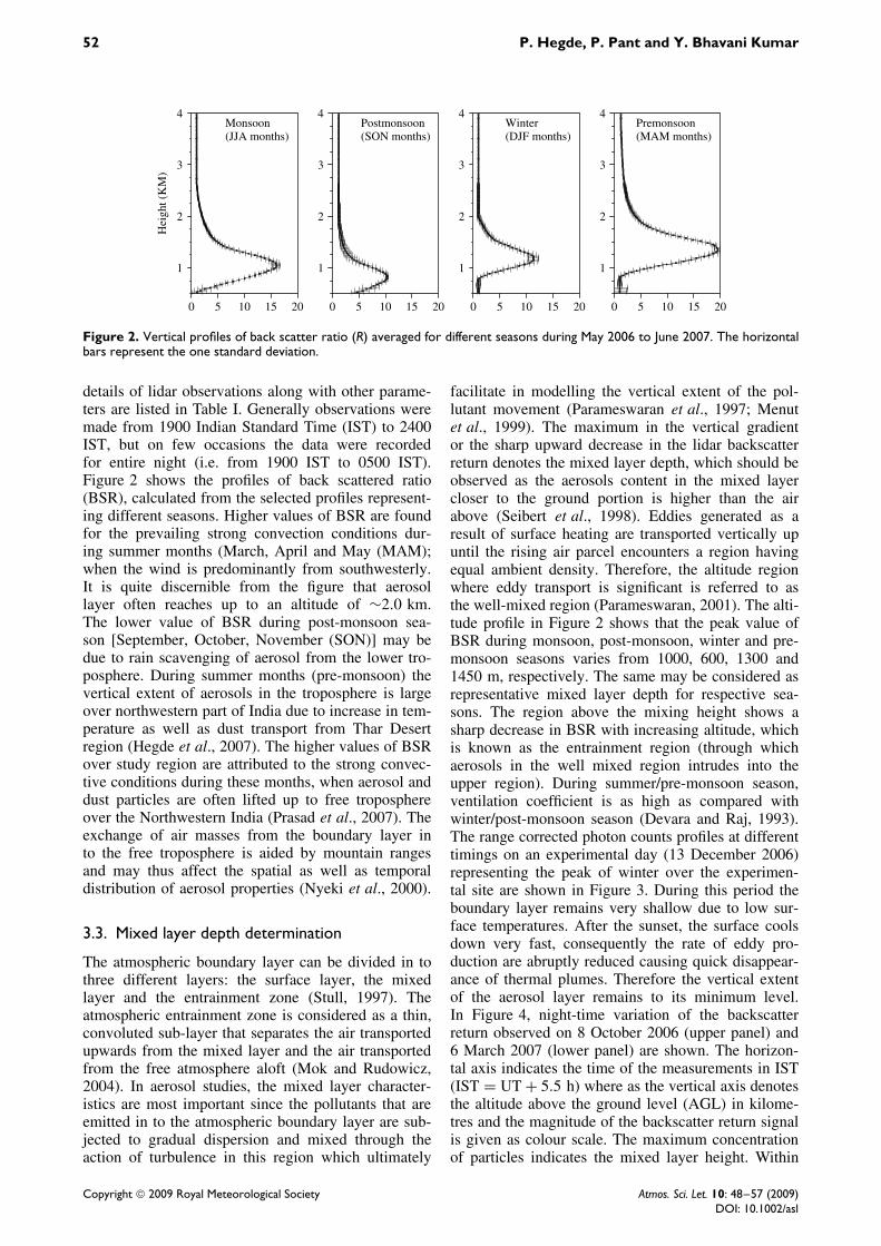
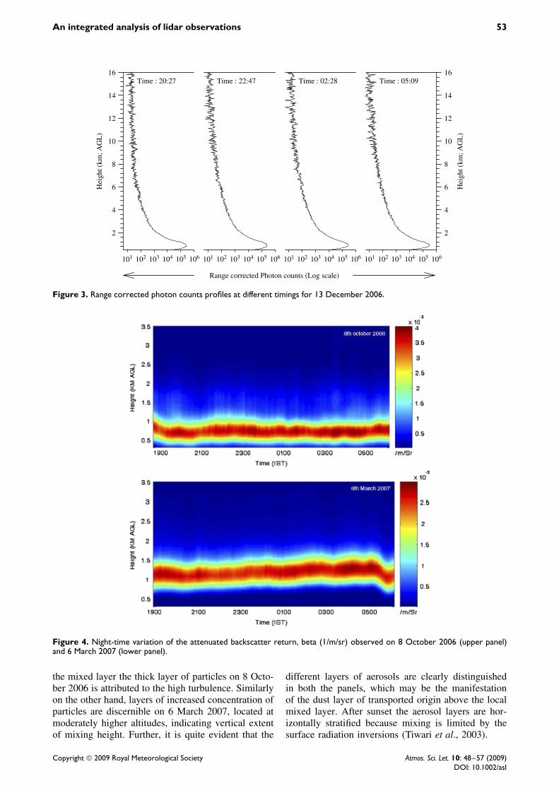
Figure 4. Night-time variation of the attenuated backscatter return, beta (1/m/sr) observed on 8 October 2006 (upper panel)and 6 March 2007 (lower panel).

the mixed layer the thick layer of particles on 8 Octo-ber 2006 is attributed to the high turbulence. Similarlyon the other hand, layers of increased concentration ofparticles are discernible on 6 March 2007, located atmoderately higher altitudes, indicating vertical extentof mixing height. Further, it is quite evident that the

different layers of aerosols are clearly distinguishedin both the panels, which may be the manifestationof the dust layer of transported origin above the localmixed layer. After sunset the aerosol layers are hor-izontally stratified because mixing is limited by thesurface radiation inversions (Tiwari et al., 2003).



3.4. Aerosol sourcesThe geographical and climatological features of theobservation site mainly determine aerosol character-istics. With the beginning of the summer, over theobserving site, the wind direction shifts from south-easterly to southwesterly, consequently the air massshifts from southern Indian plains (during winter) tothe western arid landmass (during summer). The aridlandmass includes the Great Indian Thar Desert alongthe northwestern border of India, which is one of themajor sources of atmospheric dust over the Indiansubcontinent. As the summer approaches, the north-ern and northwestern India experiences frequent duststorms due to southwesterly summer winds from thewestern Thar Desert (Sikka, 1997). In this processthe wind, arriving from Thar Desert region, bringsthe dust particles, which is mainly responsible forthe rapid enhancement in the columnar aerosol opti-cal depths (AOD) as observed over the station afterMarch. Meanwhile the higher dust concentration overthe region further reinforces the dryness of affectedregion by suppressing convection (Rosenfeld et al.,2001), which has also observed in the present study.

The annual variation in the lidar derived AOD at532 nm, varied from 0.023 to 0.264 during monsoonand summer seasons, respectively (Table I). Similartrend of temporal variation of AOD values was alsoobserved from Microtops II Sunphotometer (AOD at500 nm). The higher AOD values during summer 2006is found, mainly due to the frequent dust storms orentrainment of coarse particles over the observing siteas synoptic air mass that flows southwesterly duringMay and June results in frequent dust loading overnorthwestern part of India. On the basis of satellitedata analysis, Li and Ramanathan (2002) have alsoshown the eastward transport of west Asian desertsaerosols across the northern Arabian Sea towards thewest coast of India. The lower AOD values observedduring summer 2007 may be due to the intermit-tent rains during May 2007. Niranjan et al. (2007)have observed the mixing of the anthropogenic aerosolover the Indo-Gangetic plains with the aerosols ofdesert origin. Satheesh and Srinivasan (2002) havealso reported the enhanced values of AOD during sum-mer months over Kashidhoo and Minicoy locations,attributing the transportation of dust particles formarid regions surrounding the Arabian Sea. The min-imum AOD observed during winter months may bedue to weak-generation mechanisms and lesser possi-bility of hygroscopic growth of aerosols because oflow water vapour content in the atmosphere (Pantet al., 2006). During winter months the temperatureremains minimum over Indo-Gangetic plains causinga low-level existence of boundary layer height dueto capping inversion as well as minimum ventilationcoefficient, inhibiting the transport of particles to thefree troposphere (Nair et al., 2007). Meanwhile, thehigh value of TOMS aerosol index (AI) found overthe study region, indicates the presence of coarse par-ticles in the atmosphere. Further, the monthly mean

of AI follows the observed trend in AOD as well asBSR variations over the experimental site. This sea-sonal cycle in TOMS AI corresponds to the seasonalvariability in dust or biomass burning emissions aswell as rainfall (Habib et al., 2006).

The analysis of back trajectories at 3000 m amslduring the study period indicates when the air massoriginates from Arabian region, i.e. the trajectoriesarriving from the SW direction of the study location(Table I), generally higher values of the backscatteringas well as AOD values are observed over the site.While in the rest of the cases, the air parcel could beeither from Indian subcontinent or from the Bay ofBengal region.

3.5. Comparison with radiosonde measurements

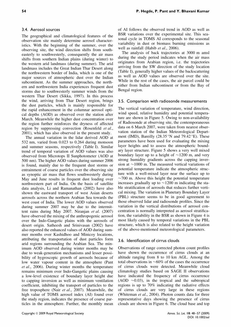
The vertical variation of temperature, wind direction,wind speed, relative humidity and potential tempera-ture are shown in Figure 5. Owing to non-availabilityof Radiosonde at observing site, the contemporaneousdata on 6 March 2007, were taken from nearest obser-vation station of the Indian Meteorological Depart-ment (IMD), Bareilly (28.35 ◦N and 79.42 ◦E). Theseparameters have been used for evaluating the mixinglayer heights and to assess the atmospheric bound-ary layer structure. Figure 5 shows a very well mixedboundary layer up to a height of ∼1200 m, and verystrong humidity gradients across the capping inver-sion at ∼1000 m. The measured vertical variations ofpotential temperature indicate the atmospheric struc-ture with a well-mixed layer near the surface up to∼700 m. Above this height the potential temperatureincreases gradually up to ∼1200 m indicating the sta-ble stratification of aerosols that reduces further verti-cal mixing. The variation in Planetary Boundary Layer(PBL) structure seems to be in good agreement tothose observed lidar and radiosonde profiles. Since thevariation in the vertical distributions of aerosol con-centration is normally interpreted as aerosol stratifica-tion, the variability in the BSR as shown in Figure 4 ismost likely caused by temporal variations in the PBLstructure, which is also related to the height variationof the above-mentioned meteorological parameters.

3.6. Identification of cirrus clouds

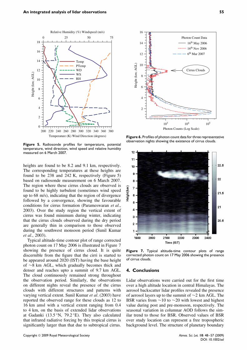
Observations of range corrected photon count profileshave shown the occurrence of cirrus clouds at analtitude ranging from 8 to 10 km AGL. Among thetotal observations in ∼60% of the cases the occurrenceof cirrus clouds were detected. Meanwhile cloudclimatology studies based on SAGE II observationshave indicated the frequency of cirrus occurrence(AOD ∼0.03), in the tropical and the subtropicalregions is up to 70% indicating the radiative effectsof cirrus clouds are very large in these regions(Whiteman et al., 2004). Photon counts data for threerepresentative days showing the presence of cirrusclouds are shown in Figure 6. The cloud base and top



Temperature (K) Wind Direction (degrees)

200 220 240 260 280 300 320 340 360 380

Hei

ght (

km; A

GL

)

0

2

4

6

8

10

12

14

16

18

TempPTempWD

Relative Humidity (%) Windspeed (m/s)

0 25 50 75

WSRH

Figure 5. Radiosonde profiles for temperature, potentialtemperature, wind direction, wind speed and relative humiditymeasured on 6 March 2007.

heights are found to be 8.2 and 9.1 km, respectively.The corresponding temperatures at these heights arefound to be 238 and 242 K, respectively (Figure 5)based on radiosonde measurement on 6 March 2007.The region where these cirrus clouds are observed isfound to be highly turbulent (sometimes wind speedup to 68 m/s), indicating that the region of divergencefollowed by a convergence, showing the favourableconditions for cirrus formation (Parameswaran et al.,2003). Over the study region the vertical extent ofcirrus was found minimum during winter, indicatingthat the cirrus clouds observed during the dry periodare generally thin in comparison to those observedduring the southwest monsoon period (Sunil Kumaret al., 2003).

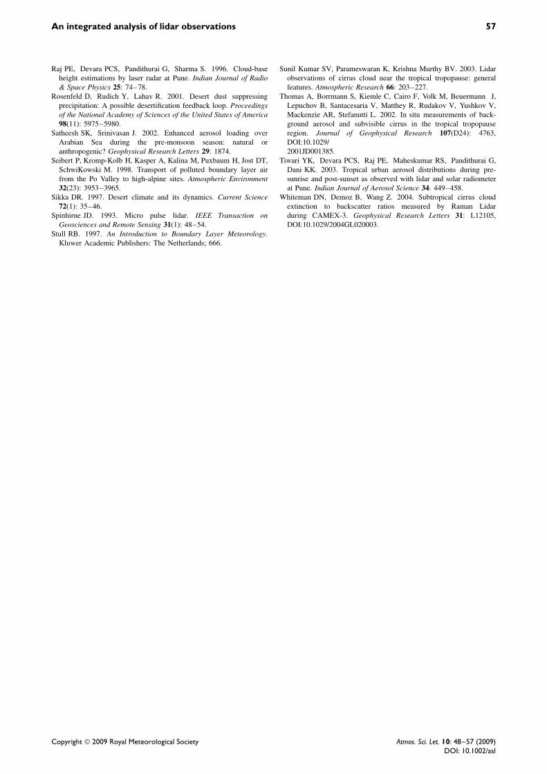
Typical altitude-time contour plot of range correctedphoton count on 17 May 2006 is illustrated in Figure 7showing the presence of cirrus cloud. It is quitediscernible from the figure that the cirri is started tobe appeared around 2020 (IST) having the base heightof ∼8 km AGL, which gradually becomes thick anddenser and reaches upto a summit of 9.7 km AGL.The cloud continuously remained strong throughoutthe observation period. Similarly, the observationson different nights reveal the presence of the cirrusclouds with different structures and patterns withvarying vertical extent. Sunil Kumar et al. (2003) havereported the observed range for these clouds as 12 to16 km amsl with a vertical extent ranging from 0.4to 4 km, on the basis of extended lidar observationsat Gadanki (13.5 ◦N, 79.2 ◦E). They also calculatedthat infrared radiative forcing by this tropical cirrus issignificantly larger than that due to subtropical cirrus.

Photon Count Data

Photon Counts (Log Scale)

103 104 105

Hei

ght (

km; A

GL

)

2

4

6

8

10

12

14

16

16th May 2006

16th Nov 2006

6th Mar 2007

Cirrus Clouds

Figure 6. Profiles of photon count data for three representativeobservation nights showing the existence of cirrus clouds.

Figure 7. Typical altitude-time contour plots of rangecorrected photon count on 17 May 2006 showing the presenceof cirrus clouds.

4. Conclusions

Lidar observations were carried out for the first timeover a high altitude location in central Himalayas. Theaerosol backscatter lidar profiles revealed the presenceof aerosol layers up to the summit of ∼2 km AGL. TheBSR varies from ∼10 to ∼20 with lowest and highestvalue during post and pre-monsoon, respectively. Theseasonal variation in columnar AOD follows the sim-ilar trend to those for BSR. Observed values of BSRover study location can represent a free troposphericbackground level. The structure of planetary boundary



layer determined from the lidar data compares rea-sonably well to those evaluated by using radiosondedata, which suggests that the lidar can be used tocharacterise the boundary layer structure. The aerosolmixing height fluctuates in the range of 600–1450 mfor post-monsoon and pre-monsoon periods respec-tively; showing a strong dependence on the verticalmixing processes of convective eddies in the atmo-spheric boundary layer due to varying meteorologicalcondition over the observing site. On several occa-sions cirrus clouds of varying thickness and durationwere successfully detected. The cloud mean altitudewas found to be ∼8 to 10 km AGL. Over the studyregion the vertical extent of cirrus was found minimumduring winter as compared to summer.

Acknowledgements

This work was carried out as a part of ABLN&C, under theISRO–GBP. Authors are thankful to the Directors, ARIESNainital, and NARL Gadanki for their encouragement toundertake this work. Thanks are due to Arjun Reddy forthe help in the lidar observations. Authors are also gratefulto anonymous reviewers for their constructive and usefulsuggestions, which significantly improved the contents of thepaper.

References

Bhavani Kumar Y. 2006. Portable lidar system for atmosphericboundary layer measurements. Journal of Optical Engineering 45(7):076201.

Cambell JR, Welton EJ, Spinhirne JD, Qiang Ji, Tsay Si-Chee,Piketh SJ, Barenbrug M, Holben BN. 2003. Micro pulse lidarobservations of tropospheric aerosol over northeastern South Africaduring the ARREX and SAFARI 2000 dry season experiments.Journal of Geophysical Research 108(D18): 33-1–33-19.

Charlson RJ, Schwartz SE, Hales JM, Cess RD, Coakley JA Jr.,Hansen JE, Hofmann DJ. 1992. Climate forcing by anthropogenicaerosols. Science 255: 423–430.

Cheng AYS, Viseu A, Leong FKC, Chan CS, Tam KS, Chan RLM.2005. Horizontal Eye-safe Mie Lidar for monitoring of UrbanAerosols in Macao. Proceedings of SPIE, Vol. 5984, Singh UN(ed.); Society of Photo-optical Instrumentation Engineers (SPIE):Washington. 59840L–1.

Devara PCS, Ernet Raj E. 1993. Lidar measurements of aerosols inthe tropical atmosphere. Advances in Atmospheric Sciences 10:365–378.

Devara PCS, Raj PE, Sharma S, Pandithurai G. 1995. Real-timemonitoring of atmospheric aerosols using a computer controlledlidar. Atmospheric Environment 29: 2205–2215.

Fernald FG. 1984. Analysis of atmospheric lidar observations: Somecomments. Applied Optics 23: 652–653.

Habib G, Venkataramana C, Chiapellob I, Ramachandran S, BoucherbO, Shekar Reddy M. 2006. Seasonal and interannual variability inabsorbing aerosols over India derived from TOMS: Relationship toregional meteorology and emissions. Atmospheric Environment 40:1909–1921.

Hegde P, Pant P, Naja M, Dumka UC, Sagar R. 2007. SouthAsian dust episode in June 2006: Aerosol observations in thecentral Himalayas. Geophysical Research Letters 34: L23802,DOI:10.1029/2007GL030692.

Immler F, Schrems O. 2002. Determination of tropical cirrus propertiesby simultaneous LIDAR and radiosonde measurements. GeophysicalResearch Letters 29(23): 2090, DOI:10.1029/2002GL015076.

IPCC. 2007. Climate Change 2007: The physical science basis,Contribution of Working Group I to the fourth assessment reportof the Intergovernmental Panel on Climate Change.

Klett JD. 1985. Lidar inversion with variable backscatter extinctionratios. Applied Optics 24: 1638–1643.

Kovalev VA. 1993. Lidar measurements of the vertical aerosolextinction profiles with range dependent backscatter to extinctionratios. Applied Optics 32: 6053–6065.

Lagrosas N, Yoshii Y, Kuze H, Takeuchi N, Naito S, Sone A, Kan H.2004. Observation of boundary layer aerosols using a continuously,portable lidar system. Atmospheric Environment 38: 3885–3892.

Li F, Ramanathan V. 2002. Winter to summer monsoon variation ofaerosol optical depth over the tropical Indian Ocean. Journal of Geo-physical Research 107(D16): 4284. DOI:10.1029/2001JD000949.

Measures RM. 1984. Laser Remote Sensing, Fundamentals andApplications. John Wiley and Sons: New York; 510.

Menut L, Flamant C, Pelon J, Flamant PH. 1999. Urban boundarylayer height determination from lidar measurements over the Parisarea. Applied Optics 38: 945–954.

Mok TM, Rudowicz CZ. 2004. A lidar study of the atmosphereentrainment zone and mixed layer over Hong Kong. AtmosphericResearch 69: 147–163.

Murayama T, Masonis SJ, Redemann J, Anderson TL, Schmid B,Livingston JM, Russell PB, Huebert B, Howell SG, McNaughtonCS, Clarke A, Abo M, Shimizu A, Sugimoto N, Yabuki M, Kuze H,Fukagawa S, Maxwell-Meier K, Weber RJ, Orsini DA, BlomquistB, Bandy A, Thornton D. 2003. An intercomparison of lidar-derivedaerosol optical properties with airborne measurements near Tokyoduring ACE-Asia. Journal of Geophysical Research 108(D23): 8651,DOI:10.1029/2002JD003259.

Nair VS, Moorthy KK, Alappattu DP, Kunhikrishnan PK, George S,Nair PR, Babu SS, Abish B, Satheesh SK, Tripathi SN, Niranjan K,Madhavan BL, Srikant V, Dutt CBS, Badarinath K VS, Reddy RR.2007. Wintertime aerosol characteristics over the Indo-GangeticPlain (IGP): Impacts of local boundary layer processes and long-range transport. Journal of Geophysical Research 112: D13205,DOI:10.1029/2006JD008099.

Niranjan K, Madhavan BL, Sreekanth V. 2007. Micro pulse lidarobservation of high altitude aerosol layers at Visakhapatnam locatedon the east coast of India. Geophysical Research Letters 34: L03815,DOI:10.1029/2006GL028199.

Nyeki S, Kalberer M, Colbeck I, De Wekker S, Furger M, GaggelerHW, Kossmann M, Lugauer M, Steyn D, Weingartner D, Wirth M,Baltensperger U. 2000. Convective boundary layer evolution to4 km asl over high-alpine terrain: Airborne lidar observationsin the Alps. Geophysical Research Letters 27(5): 689–692,10.1029/1999GL010928.

Pant P, Hegde P, Dumka UC, Sagar R, Satheesh SK, Moorthy KK,Saha A, Srivastava MK. 2006. Aerosol characteristics at a highaltitude location in central himalayas: Optical properties andradiative forcing. Journal of Geophysical Research 111: D17206,DOI:10.1029/2005JD006768.

Parameswaran K. 2001. Influence of micrometeorological features oncoastal boundary layer aerosol characteristics at the tropical station,Trivandrum. Proceedings of the Indian Academy of Sciences-Earthand Planetary Sciences 110: 247–265.

Parameswaran K, Rose KO, Krishna Murthy BV, Osborn MT, McMaster LR. 1991. Comparison of aerosol extinction profiles fromlidar and SAGE-II data at a tropical station. Journal of GeophysicalResearch 96: 10861–10866.

Parameswaran K, Sunil Kumar SV, Krishna Murthy BV. 2003. Lidarobservations of cirrus cloud near the tropical tropopause: temporalvariations and association with tropospheric turbulence. AtmosphericResearch 69: 29–49.

Parameswaran K, Vijayakumar G, Krishna Murthy BV. 1997. Lidarobservations on aerosol mixing height in a tropical coastalenvironment. Indian Journal of Radio & Space Physics 26: 15–21.

Prasad AK, Singh S, Chauhan SS, Srivastava MK, Singh RP, Singh R.2007. Aerosol radiative forcing over the Indo-Gangetic plains duringmajor dust storms. Atmospheric Environment 41(29): 6289–6301.



Raj PE, Devara PCS, Pandithurai G, Sharma S. 1996. Cloud-baseheight estimations by laser radar at Pune. Indian Journal of Radio& Space Physics 25: 74–78.

Rosenfeld D, Rudich Y, Lahav R. 2001. Desert dust suppressingprecipitation: A possible desertification feedback loop. Proceedingsof the National Academy of Sciences of the United States of America98(11): 5975–5980.

Satheesh SK, Srinivasan J. 2002. Enhanced aerosol loading overArabian Sea during the pre-monsoon season: natural oranthropogenic? Geophysical Research Letters 29: 1874.

Seibert P, Kromp-Kolb H, Kasper A, Kalina M, Puxbaum H, Jost DT,SchwiKowski M. 1998. Transport of polluted boundary layer airfrom the Po Valley to high-alpine sites. Atmospheric Environment32(23): 3953–3965.

Sikka DR. 1997. Desert climate and its dynamics. Current Science72(1): 35–46.

Spinhirne JD. 1993. Micro pulse lidar. IEEE Transaction onGeosciences and Remote Sensing 31(1): 48–54.

Stull RB. 1997. An Introduction to Boundary Layer Meteorology.Kluwer Academic Publishers: The Netherlands; 666.

Sunil Kumar SV, Parameswaran K, Krishna Murthy BV. 2003. Lidarobservations of cirrus cloud near the tropical tropopause: generalfeatures. Atmospheric Research 66: 203–227.

Thomas A, Borrmann S, Kiemle C, Cairo F, Volk M, Beuermann J,Lepuchov B, Santacesaria V, Matthey R, Rudakov V, Yushkov V,Mackenzie AR, Stefanutti L. 2002. In situ measurements of back-ground aerosol and subvisible cirrus in the tropical tropopauseregion. Journal of Geophysical Research 107(D24): 4763,DOI:10.1029/2001JD001385.

Tiwari YK, Devara PCS, Raj PE, Maheskumar RS, Pandithurai G,Dani KK. 2003. Tropical urban aerosol distributions during pre-sunrise and post-sunset as observed with lidar and solar radiometerat Pune. Indian Journal of Aerosol Science 34: 449–458.

Whiteman DN, Demoz B, Wang Z. 2004. Subtropical cirrus cloudextinction to backscatter ratios measured by Raman Lidarduring CAMEX-3. Geophysical Research Letters 31: L12105,DOI:10.1029/2004GL020003.


Documents

An integrated analysis of lidar observations in association with optical properties of aerosols from a high altitude location in central Himalayas