An integrated in-silico gene mapping strategy in inbred mice.

Alessandra C. L. Cervino*, Ariel Darvasi †, Mohammad Fallahi*, Christopher C. Mader*

and Nicholas F. Tsinoremas*

* Scripps Florida

Department of Informatics

Jupiter, FL 33458

USA

† The Institute of Life Sciences

The Hebrew University of Jerusalem

Jerusalem, 91904

ISRAEL

Genetics: Published Articles Ahead of Print, published on October 8, 2006 as 10.1534/genetics.106.065359

An integrated gene mapping strategy in mice.

SNP, IBD, mice, QTG, in-silico

Alessandra C. L. Cervino

Department of Informatics

Scripps Florida

5353 Parkside Drive, RF-A

Jupiter, FL 33458

Telephone: 561-799-8928

Facsimile: 561-799-8952

E-mail: cervino@scripps.edu

ABSTRACT

In recent years in-silico analysis of common laboratory mice has been introduced and

subsequently applied, in slightly different ways, as a methodology for gene mapping.

Previously we have shown some limitation of the methodology due to sporadic genetic

correlations across the genome. Here, we revisit the three main aspects that will affect in-

silico analysis. First, we report on the use of marker maps: we compared our existing 20k

SNP map to the newly released 140k SNP map. Second, we investigated the effect of

varying strain numbers on power to map QTLs. Third, we introduced a novel statistical

approach: a cladistic analysis, which is well suited for mouse genetics and has increased

flexibility over existing in-silico approaches. We have found that in our examples of

complex traits, in-silico analysis by itself does fail to uniquely identify QTG containing

regions. However, when combined with additional information it may significantly help

to prioritize candidate genes. We therefore recommend using an integrated workflow that

uses other genomic information such as linkage regions, regions of shared ancestry and

gene expression information to get from the genome to a list of candidate genes.

INTRODUCTION

The mouse represents one of the most commonly used model organisms in science. Its

fast breeding rate, the ability to control the environment it lives in and the ability to

control its genetic background, make it the ideal organism to study the genetics of a

multitude of traits and diseases. To date the most commonly used approach to identify

genes underlying traits (QTG) using mice is linkage analysis, a method that consists in

crossing generally two strains. Then by studying the recombinations in the following

generation(s) one can identify large regions potentially containing QTG. Those regions

get subsequently analysed in greater detail using further mice, a process that takes years

to get to the gene(s) and is rarely successful, see (FLINT et al. 2005) for a recent review.

Narrowing QTL regions still remains a “major challenge” (MOTT 2006). In 2001 (GRUPE

et al. 2001) illustrated how an alternative approach, based on comparing phenotypes from

different strains, could be applied to gene mapping. Although their initial approach was

based on a rather small number of genotypes and strains, it did open the way to a novel

approach, which, simply put, tests for association between a trait and a genotype treating

different strains of mice as individuals from a population. The approach is intuitive. Its

chance of success, as initially applied, however, is debatable (DARVASI 2001).

Over the last few years reports have started to appear using in one way or another

the idea of in-silico analysis to identify genes (CERVINO et al. 2005; HILLEBRANDT et al.

2005; PLETCHER et al. 2004). Significant efforts have resulted in the release of large

amounts of genotyped single nucleotide polymorphisms (SNPs) in inbred strains

(CERVINO et al. 2005; WADE and DALY 2005; WILTSHIRE et al. 2003). Phenotypic

information has also become increasingly available through public databases (for

example: the Phenome database, the Eumorphia project). As a result, many in-silico

projects are ongoing and many more are being planned. It is therefore timely to revisit

some of the strengths and limitations of an in-silico based approach.

The goal of in-silico analysis is to identify if not a gene, a short genomic region or

list of candidate genes containing a gene influencing the trait under study. To

successfully achieve this goal many factors need to be considered: the trait under study

and its genetic component, the number of strains used in the in-silico experiment, the

number of genetic markers used in the in-silico analysis and the statistical algorithms

used in the analysis. Here we investigated the effect of these factors on both experimental

and simulated datasets. First, we looked at the effect of using a 20k SNP map versus the

140k SNP beta map just released by (WADE and DALY 2005), which we refer to as the

BROAD/MIT data. Second, we investigated the effect of strain numbers on the power to

map QTLs using simulated traits as well as the cholesterol phenotype. We selected the

cholesterol phenotype because it had been measured in the largest number of strains.

Third, we implemented a novel analysis to test for association between haplotypes of

varying lengths and traits and compared it to a number of different algorithms on both

mendelian and complex traits. The underlying assumption to our cladistic model, that

similar haplotypes correspond to similar disease risks, is particularly well suited to the

field of mouse genetics where common laboratory strains all come from a very limited

number of founders. This type of analysis takes into account the genetic proximity

between related strains, handles missing data, allows for repeated measures and is fully

flexible as it can be used to model different families of distributions. Finally, we illustrate

the use of an integrated strategy that combines information from linkage analysis, blocks

of shared ancestry (IBD-Identical By Descent), in-silico analysis and gene expression.

Our strategy when applied to complex traits, results in successfully narrowing down the

entire genome to a handful of candidate genes.

MATERIALS AND METHODS

IBD database

Genotypes from 48 strains were downloaded as text files from the BROAD/MIT website

and imported into our in house database. IBD regions were then estimated by identifying

regions of at least 1Mb between any two strains without informative SNPs (CERVINO et

al. 2006). The images from the 140k map were added to our existing website which

previously contained IBD information on 61 strains using about 20k SNPs. Both the 20k

and the 140k set map to the mouse genome build NCBIM33. For the purpose of

comparing the 20k map to the 140k map, we assumed that BALB/cJ which was used in

our existing database and BALB/cByJ which was part of the BROAD/MIT list of strains

were the same strains.

In-silico methods

Statistical algorithms: To test for genetic association with any given trait we used 4

different algorithms, one S20 or S140 (# refers to the number of SNPs used) tests for

association between a genotype and a trait, the other three algorithms test for association

between a haplotype and a trait using a cladistic model: C20.3 or C140.3, C20.10 or

C140.10 and C20.sli or C140.sli.

- S#: Single point marker analysis. It returns the p-value from a Student t-

test when the data is continuous or a chi-square if the data is binary. Since

the markers are SNPs and the strains are all inbred, only two groups

corresponding to the two different alleles exist at each position.

- C#.3: Cladistic analysis using a haplotype of 3 consecutive SNPs. Starting

at each position the first three SNPs are assembled to define a haplotype, a

measure of genetic distance between the haplotypes is calculated as the

number of alleles differing between each haplotypes, then a tree (using

the hierarchical function hclust in the R language) is built on the

haplotypes that then define new groups. At each branch of the tree a test is

performed using general linear models with a Gaussian link or a binomial

link depending on whether the data is continuous or binary. The P-value is

obtained from comparing the null model of no association with the

alternative model of association with the groups as an independent

variable, the chi-square statistic is used. The algorithm is applied at each

SNP position, consecutive haplotypes therefore overlap by 2 SNPs.

- C#.10: Cladistic analysis using a haplotype of 10 consecutive SNPs. Same

as C#.3 except the haplotypes blocks are longer as they are based on 10

SNPs. The algorithm is applied at each SNP position, consecutive

haplotypes therefore overlap by 9 SNPs.

- C#.sli: Cladistic analysis using a haplotype of however many SNPs are

present in a 100kb window. Same as C#.3 except that the haplotypes are

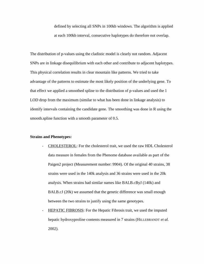
defined by selecting all SNPs in 100kb windows. The algorithm is applied

at each 100kb interval, consecutive haplotypes do therefore not overlap.

The distribution of p-values using the cladistic model is clearly not random. Adjacent

SNPs are in linkage disequilibrium with each other and contribute to adjacent haplotypes.

This physical correlation results in clear mountain like patterns. We tried to take

advantage of the patterns to estimate the most likely position of the underlying gene. To

that effect we applied a smoothed spline to the distribution of p-values and used the 1

LOD drop from the maximum (similar to what has been done in linkage analysis) to

identify intervals containing the candidate gene. The smoothing was done in R using the

smooth.spline function with a smooth parameter of 0.5.

Strains and Phenotypes:

- CHOLESTEROL: For the cholesterol trait, we used the raw HDL Cholesterol

data measure in females from the Phenome database available as part of the

Paigen2 project (Measurement number: 9904). Of the original 40 strains, 38

strains were used in the 140k analysis and 36 strains were used in the 20k

analysis. When strains had similar names like BALB.cByJ (140k) and

BALB.cJ (20k) we assumed that the genetic difference was small enough

between the two strains to justify using the same genotypes.

- HEPATIC FIBROSIS: For the Hepatic Fibrosis trait, we used the imputed

hepatic hydroxyproline contents measured in 7 strains (HILLEBRANDT et al.

2002).

- BLINDNESS: For the blindness phenotype we used 37 strains for the 20k

analysis and 46 strains for the 140k analysis. The binary traits were obtained

from the Jackson laboratory and were the same that had been previously

analysed (PLETCHER et al. 2004).

- ALBINISM: For the albinism phenotype, we used the 12 strains reported in

(WADE et al. 2002). The trait for albinism is binary.

- SIM1QTL: This simulated trait represents a single SNP model. The

‘causative’ SNP was randomly selected from the 140k map and maps to 93Mb

on chromosome 14. The trait was simulated in 41 strains, which corresponds

to the number of strains that had been genotyped at that SNP. Under our

model the mean for the two alleles were 0 and 1 with a standard deviation of

0.01, such a strong effect is similar to a mendelian trait. SIM1delQTL is the

same trait, but we removed the causative SNP from the 140k map when

performing the analysis.

- SIM2QTL: This trait was simulated using the following algorithm: 2 SNPs

were selected at random from the 20k SNPs. For each SNP the first

encountered allele was selected as the risk allele and increased the trait

(baseline level was set to 0) by 0.5. This 2 SNP model represents an additive

model that fully explains all of the trait variation. For example the trait for a

strain with no risk allele was set to 0, strains with two risk alleles were set to

1. The trait values were then transferred to the strains represented in the 140k

map. The trait was simulated in 35 strains for the 20k analysis and resulted in

33 strains for the 140k analysis. The 2 QTLs mapped to chromosomes 3 and

12.

RESULTS

The effect of SNP maps

Previously we had assembled public genotypes from 21,514 SNPs in 61 strains of mice

(CERVINO et al. 2006), we refer to these genotypes as the 20k SNP map. The 140k SNP

map corresponds to the beta release data from the BROAD/MIT, this corresponds to

138,793 SNPs genotyped in 49 strains (WADE and DALY 2005). The same assembly

(mouse genome build NCBIM33) was used in both maps. We looked at the effect of

using the 140k SNP map versus the 20k map on estimating IBD blocks as well as on the

in-silico analysis.

IBD database: The Scripps Florida IBD database provides estimates of SNP poor

regions corresponding to areas of shared ancestry between pairs of strains based on 61

common strains that had been genotyped in about 20K SNPs (CERVINO et al. 2006).

When using 20K SNPs only large blocks of about 1Mb could be reasonably well

estimated. Clearly the IBD blocks can be more accurately estimated using additional

genotypes, we therefore re-computed the IBD blocks using the 140K genotypes from 48

strains and updated our database with the estimated positions of the new IBD blocks. We

also updated our website with the corresponding images.

Thirty five strains were common to both datasets. Based on those 35 strains we

compared the estimated IBD blocks and found that in general there was good agreement

between the two maps. Closely related strains showed the least differences in block

estimates and more distant strains showed the greatest differences. Fewer blocks were

identified when using the 140k map between distant strains

(http://mouseibd.florida.scripps.edu). For example, the overall amount of IBD on

chromosome 10 between A and CZECH dropped from 23% to 12%. Looking at closely

related strains such as 129S1 and 129X1, we noted that ‘SNP singletons’, ie individual

SNPs situated in large areas of IBD blocks were not present when using the 140k

genotypes. Going back to the original SNP data we found that most such singletons were

submissions from GNF and that those genotypes were not in agreement with genotypes

from other experiments, making us conclude that those singletons were genotyping errors

and that the quality of the BROAD/MIT genotypes and the Merck genotypes are of

greater quality than the GNF published genotypes.

In-silico Analysis: To assess the effect of using the two different maps, we compared the

results from a single marker analysis as well as a novel clade based analysis using a 3

SNP haplotype (see Methods). We used two mendelian traits as positive controls: the

albinism phenotype which is caused by a mutation at the tyrosinase locus (YOKOYAMA et

al. 1990) and the blindness phenotype which is caused by a mutation in the Pde6b gene.

For albinism the phenotype from 12 strains was used (WADE et al. 2002), for blindness

48 strains were used (PLETCHER et al. 2004).

For the albinism phenotype, we report the p-values at each SNP on the 19

autosomal chromosomes as well as the p-values based on the cladistic analysis. 12 inbred

strains were used. Figure 1a represents –log of the p-value for each marker along all 19

chromosomes using the 20k map at the top and using the 140k map at the bottom. Figure

1b represents –log of the p-value using a 3 SNP window (plotted at the start of the

window) along all 19 chromosomes using the 20k map at the top and using the 140k map

at the bottom.

Figures 1 show that chromosome 7 is correctly identified among the markers with

the highest p-value in both maps. However, there are more significant markers when

using the 140k map (which is to be expected given the increase in number of tests

performed), which leads to a higher rate of false positives (if selecting based on

maximum p-value). When using a single marker analysis (Figure 1a) 8 out of 19

chromosomes are among the markers with the highest p-value, when using the 140k map

this goes up to 9 out of 19. Using the cladistic analysis the number of chromosomes with

association is 9/19 for the 20k map, and 10/19 for the 140k map. At the chromosome

level, we therefore see no gain from increasing the map resolution in this case. If one did

not have prior linkage data to identify the correct chromosome carrying the QTG, one

would have to search half of the chromosomes. This illustrates the importance of

combining classical QTL analysis with in-silico analysis. Given a small number of strains

like 12 (which is pretty standard for in-silico analysis) an in-silico only based analysis

would pick up the right chromosome along with half of the other chromosomes that make

up the mouse genome. However combined with the knowledge from classic linkage

analysis, one knows that the correct chromosome is chromosome 7 and when looking at

chromosome 7 in further detail (Figures 2) one can correctly identify the location of the

underlying gene. The position of the tyrosinase gene is represented by a red vertical bar.

As is apparent from Figures 2, using the 20k map markers in the neighbourhood of the

genes have the most significant p-values, this is also the case using the 140k map.

However, there are more associated markers when using the 140k map which is to be

expected given the overall increase in number of markers. As noted at the genome wide

level, there is no benefit in this case from using the 140k map over the 20k map.

For the blindness phenotype, we did the same as for the albinism trait and

calculated the p-values at each SNP on the 19 autosomal chromosomes as well as the p-

values based on the cladistic analysis (Figures 3). For the 20k map based analysis, 37

strains were used whilst for the 140k map, 46 strains were used. Chromosome 5 is

correctly identified as the only chromosome with the highest p-value using either map,

and either method. No other chromosome has an association more significant than 10-6.

Compared to the albinism phenotype, this case has a larger sample size (around 40 strains

instead of 12), which leads to smaller p-values and hence one is able to distinguish the

correct chromosome from the others. It therefore, appears that having large numbers of

strains is key to identifying a chromosome when no prior linkage data is available. This

will be further investigated in the section “The effect of strain numbers”. When looking

at chromosome 5 only (Figures 3), again the two maps lead to the same conclusion since

they identify the genomic area in the region of the gene (indicated by a red bar).

When using the strongest p-value to select chromosomes or candidate regions, we

do not see any gain from using the 140k map compared to the 20k map when performing

in-silico analysis on simple mendelian traits.

The effect of strain numbers

When planning in-silico experiments, it is important to estimate the number of strains

required to achieve a certain level of power. (WANG et al. 2005) looked at the effect of

strain numbers on power under varying genetic models and for varying numbers of

haplotypes. In their example, a sample size of 10 was only really powerful when looking

at very strong genetic effects such as mendelian traits. For a trait with a genetic effect

contributing in the range of 30% to the total variance, 30 strains or more are required for

acceptable power. In real examples of complex traits the genetic contribution is much

lower than that figure of 30%. To look at the effect of strain numbers on mapping power

we analysed subsets of simulated data as well as real data. We simulated two datasets

(see methods) the first simulated trait, SIM1QTL, corresponds to a single high risk allele,

the second trait, SIM2QTL, was generated assuming two causative SNPs situated on

different chromosomes with equal risk and an additive effect. As an example of real data,

we selected the cholesterol trait, since HDLC levels was the phenotype that had been

measured in the largest number of strains (n=38). For both simulated and real traits, we

then randomly selected 100 subsets of 30, 20 and 10 strains and applied our cladistic

analysis of size 3 followed by spline smoothing to investigate how often the correct QTL

region was identified as the most likely region. We defined a 5Mb interval around the

SNP or gene as the QTL region and only tested the chromosomes where the QTL was,

based on the results from the previous section. The results are presented in Table 1. There

is a dramatic loss of power as the traits become complex and the genetic effect decreases.

Interestingly, whether the causative SNP is included in the map (SIM1QTL versus

SIM1delQTL) does not affect power, highlighting the strength of our analytical approach

and the informativeness of existing maps. The power decreases proportionally to the

number of strains. Surprisingly, in our simulated example of two additive SNPs with

extremely large effects, we completely fail to identify the first SNP and the mapping of

the second SNP is a few Mb off. The two loci (SIM2QTLs) were simulated using the

same procedure and were both absent in the 140k map. The difference in the statistical

power between the two loci is therefore most likely due to the number of informative

SNPs at neighbouring makers and to the distance to the nearest markers. A different

choice of markers would have led to a difference in power. When we simulated traits

with 3-5 underlying QTLs, none or only one QTL was identified using 30 strains (data

not shown). With less than 30 strains or with equal additive multigenic effects there is

little rationale supporting an in-silico analysis of complex traits. It is therefore important

when planning in-silico analysis to get an accurate estimate of the number of QTLs

involved and their associated risks. After that, one should target a corresponding

minimum number of strains or use a different strategy such as the one described later.

Since our analytical approach is based on 3 SNP haplotypes, we would expect it to

perform better in classical inbred strains as opposed to wild derived strains since the

causative SNP is more likely to be represented on the same haplotypes. To investigate if

there was a loss of power associated with including wild derived strains in the in-silico

analysis, we compared the group of sets that correctly mapped the QTL to the frequency

of wild derived strains in our simulated data. If the inclusion of wild derived strains had

resulted in loss of power, then we would have expected an overrepresentation of wild

strains in the random subsets that failed to map the QTL. In our simulated data we did not

see any evidence for a loss of power associated with including the wild strains in the

analysis. For example, the average number of wild strains in the 93 groups of 30 strains

that successfully mapped the single QTL (SIM1QTL) was 3.7 compared to 3.3 in the 7

groups of 30 strains that failed to map the same QTL.

The effect of statistical algorithms

In in-silico analysis, one tests for association between a trait and a genetic marker in a

population of inbred strains. (CERVINO et al. 2005) tested for association between

individual SNPs and the trait of interest, (PLETCHER et al. 2004) and (HILLEBRANDT et al.

2005) used a haplotype defined by a 3 SNP window. Here, we have implemented for the

first time a cladistic analysis to test for association between a trait and haplotypes of sizes

3 SNPs, 10 SNPs and of length 100kb. Given the recent shared history of most of the

laboratory mice, applying a cladistic analysis to this type of data is a natural choice. The

cladistic analysis is a haplotypic analysis, where the haplotypes get merged into groups in

a stepwise fashion (See Figure 4). The cladistic approach will be especially successful

when the risk carrying mutation is fully associated with a single haplotype. Such a

situation is most likely to be the case in laboratory mice since they were derived from a

limited number of founders. This method has been applied to human populations

(DURRANT and MORRIS 2005; DURRANT et al. 2004) with increased power when

compared to more standard methods, but was never implemented to study inbred mice.

Because laboratory mice are inbred, their haplotypes are known.

To assess the performance of the cladistic analysis, we compared single marker

analysis to the cladistic analysis with windows of sizes 3, 10 and of length 100kb on four

traits: 2 mendelian traits and 2 complex traits with known or strong candidates. We report

the results for the 140k maps, since we would assume that most scientists would use the

denser map, results for the 20k map are available from the authors upon request.

The ultimate goal of the statistical analysis is not to identify an association with a

marker but to estimate the most likely position of the risk carrying gene. To that end, we

implemented the following approaches: For the single marker analysis we report the

position of the first and last markers that correspond to the minimum p-value at the

selected chromosome. For the cladistic analysis we applied two approaches, first we

report the positions of the most strongly associated haplotypes at the selected

chromosome. The second approach is based on the p-values resulting from the cladistic

analysis. For each SNP position along the chromosome, a p-value is calculated from

testing for association between a clade and the trait. The resulting distribution of p-values

along the chromosome is a not random distribution. Given the correlation between

adjacent p-values, we assumed that applying a smoother would help us in estimating the

interval containing the QTG. Smoothing does allow the extrapolation to a continuous

scale, ie we have information at every position not just where the SNPs are and it favors

associations with multiple windows over single isolated associations, which we

intuitively felt more convincing. We therefore used a 1 LOD drop in the distribution of

the p-values after fitting a smoothed spline (see methods). We chose to apply a spline

which is a non parametric smoother since the true distribution of the p-values is not

known. The results are reported in Table 2.

The first thing that one notices is that for the two Mendelian phenotypes

(blindness and albinism), all algorithms map the association within 1Mb of the

underlying gene. Different methods are closer or further away from the gene and have

intervals of varying length for estimating the gene position. Application of the spline

smoother results in larger confidence intervals for the blindness traits when compared to

using the raw haplotype based p-values. However, when multiple haplotypes are

associated with the trait, as is the case for the albinism trait (Figures 5), the application of

a smoother to the distribution of p-values results in tighter intervals.

Overall the application of a “spline smoother” to the p-value distribution results in

intervals from 2Mb to 14Mb with an average of about 5 Mb which are relatively large

intervals, although they are considerably smaller than intervals from linkage analysis.

When looking at the results from the analysis of complex traits such as cholesterol level

and hepatic fibrosis, one notices that different methods map the most significant

association to different parts of the chromosome. HDLC cholesterol and hepatic fibrosis,

each have genes that are known to influence the traits. For cholesterol, it is Apoa2

(HEDRICK et al. 2001; SUTO 2006; WANG and PAIGEN 2002), other genes have also been

mapped to the same chromosome (CERVINO et al. 2005; WANG et al. 2003), which will

influence the analysis and decrease the power to identify ApoA2. Based on RI sets

(NxSM), 74% of the HDL-C variance can be explained by that locus (MEHRABIAN et al.

1993), in an independent F2 cross (B6xRR) ApoA2 was found to explain 33.1% of the

variance (SUTO et al. 2004). For hepatic fibrosis two QTLs have been identified that

explain 2-5% of the total variance (HILLEBRANDT et al. 2002), subsequently the second

QTL was narrowed down to a QTG: Hc (HILLEBRANDT et al. 2005). Only the cladistic

analysis with a window of size 3 followed by spline smoothing identifies the position

within 1Mb of the location of those genes, the cladistic analysis with windows of length

100kb estimates the position of Hc just over 1Mb away whilst the other methods identify

other regions. Both the single point analysis and the cladistic analysis of haplotypes of

size 3 alone failed to identify either regions.

From these examples, it appears that the cladistic analysis of size 3 with spline

smoothing is the best performing algorithm followed closely by the cladistic analysis of

100kb haplotypes with spline smoothing. The intervals when applying the smoothing

technique on the p-values and the use of a 1 LOD drop do result in larger intervals than

when using a single marker or haplotype based analysis when there is a single marker or

a single haplotype with the strongest association. However when there are multiple

haplotypes or single markers with the same level of association, and in different parts of

the chromosome, one has no way of differentiating which one is more likely to be the

true one. Fitting a spline to smooth the distribution of the p-values, as we present here for

the first time, does have the advantage that observations from nearby SNPs are all

contributing to the calculations thereby helping to identify the true genomic region

containing the underlying gene.

Gene mapping in complex traits: an integrated approach

As we have just shown, in-silico analysis by itself performed on a limited number of

strains will most likely fail at identifying the correct region underlying complex traits. To

help with the gene mapping process, it is therefore necessary to bring information from

multiple sources such as: linkage data, IBD information and gene expression. We will

now illustrate how this integrated approach was applied to two complex traits: cholesterol

and hepatic fibrosis.

Cholesterol: To illustrate the application of our approach when using solely public data,

we chose cholesterol levels. To identify a gene influencing cholesterol levels, we used the

linkage and phenotypic data from the Jackson laboratory. Looking at their informatics

website, we selected HDL levels as a trait and select the chromosome 1 QTL as it had the

highest LOD score and had been confirmed by others (KORSTANJE and PAIGEN 2002).

The nearest marker to the peak was D1Mit291 which maps to 184.5Mb on assembly 33.

We therefore used the 170-200 Mb region as the QTL region. The F2 cross used to

identify the QTL was between SM/J and NZB/B1NJ. We investigated the IBD structure

of those two strains in the 30Mb region of chromosome 1. Three IBD blocks were

identified in that region, totaling about 6Mb, and were therefore excluded from the

candidate region. We added expression information from the GNF atlas to find the genes

present in those regions that are expressed in the liver. A total of 190 genes were found in

the candidate region (which excluded the IBD blocks). When applying a filter of 3x over

the median for liver expression, 6 genes came out as the final list of candidates: Ush2a,

Fh1, Kmo, Apoa2, Hsd17b7 and Nr1i3. Given that the in-silico analysis estimates the

position with an upper most limit at 172 (Table 2), the most likely candidates are

therefore Apoa2, Hsd17b7 and Nri3.

By combining information from QTL experiments, IBD blocks, in-silico

association study and expression analysis, we got down to a list of three candidates, one

of the three being a known cholesterol gene.

Hepatic Fibrosis: To illustrate the application of our integrated approach to data

generated in a single laboratory, we used hepatic fibrosis as an example. (HILLEBRANDT

et al. 2002) studied the genetics of hepatic fibrosis following chronic liver injury using a

mouse model where mice were treated with CCl4 . Linkage analysis was performed by

crossing BALB/cJ and A/J strains, and an association study was also done in 7 inbred

strains. The linkage analysis identified linkage regions on chromosomes 2 and 15. In their

follow up work they identified Hc as the underlying gene on chromosome 2.

We performed in-silico analysis using the latest 140k map and using the

algorithms described here. Chromosome 15 showed a strong association pattern at around

68Mb, whilst the association on chromosome 2 was much weaker. For the linkage region

on chromosome 2 we used the first 35Mb (up to D2Mit238) and for chromosome 15, we

used the region from 30-70 Mb which is around D15Mit26 and D15Mit122. Four blocks

were identified on chromosome 2. Adding the information of the in-silico results which

peaks around 30Mb, the two most likely regions are now: 18.7Mb-26.9 Mb and 30.3-35

Mb. In the 30.3-35 Mb interval 172 genes are reported in the GNF atlas, filtering with a

median fold increase of 3 for liver expression, three candidate genes exist: Ass1, Hc and

Slc25a25. Another 6 known genes were found in the 18.7-26.9Mb interval. The final list

of 9 candidate genes did, as in the cholesterol example, include the correct one,

illustrating the power of this integrated approach. On chromosome 15, four large blocks

were identified in the 30-70Mb region. With the in-silico results peaking at 68Mb, that

leaves the 58.5-70Mb as the most likely region to contain a QTG. Looking at the gene

expression information, only the following two candidate genes pass the three fold

criteria: Mtss1 and A1bg.

DISCUSSION

With the beta release of the 140k map from (WADE and DALY 2005), and the many

ongoing projects to measure phenotypes in different inbred strains, in-silico analysis is

well on its way to becoming a standard methodology for identifying genes underlying

complex traits. Under certain genetic models, like mendelian traits, it can be used by

itself, however we have found that used by itself in the complex traits presented here, it

failed to identify the correct QTG regions. We therefore concluded that in complex traits,

it is best to use in-silico analysis in conjunction with other sources of information such as

linkage analysis (RI, F2 or BC1), expression data (eQTL analysis or high expression in a

tissue of interest) and knowledge about IBD regions. The gene expression information as

well as the genotypic information are already well covered by public sources such as the

GNF and the Jackson laboratory websites. Although we did not find that the in-silico

analysis was significantly improved by using this denser map, we have found that the

IBD map from the 140k map was of higher quality than the previous 20k map which was

collected from multiple sources.

One of the interesting aspects of in-silico analysis is the statistical methodology

used to test for association. Here we introduced a novel cladistic approach to test for

association between a haplotype and a trait. We varied the haplotype’s length since fixed

window sizes are easy to compute but do lack biological meaning. We therefore used a

haplotype of length 100kb as well as fixed SNP sizes. Although intuitively we preferred

that method of determining haplotypes, there did not seem to be any increase in power

over a 3 SNP window. One could further vary the length of the haplotype depending on

the area of the chromosome, as one might benefit from having shorter haplotypes in

regions with a lot of diversity and longer haplotypes in regions that are conserved (for

example in SNP poor regions across all tested strains). Recent reports that have

investigated the length of haplotype blocks in mice could be used to help determining the

optimal haplotype length, e.g. (ADAMS et al. 2005; FRAZER et al. 2004; WADE et al.

2002; YALCIN et al. 2004). The advantage of the cladistic approach is that it naturally

seems to apply to inbred mice since it builds a tree based on the genetic distances and

hence it recreates the phylogeny of the strains for that particular region, which is a better

approach than specifying what the distance is based on the whole genome. The use of a

statistical framework has the added benefit of allowing more complex analyses. Missing

genotypic data are handled appropriately, and methods such as repeated measures models

can easily be implemented taking into account the intra strain variation. In our examples

we tried to correctly identify the positions of known genes. Except in our simulated data,

we focused mostly on single gene analysis and the most significant p-value, in the case of

complex traits, however, there are multiple genes that contribute to the trait. In the future

it would be interesting to assess, once there is such a list of validated genes contributing

to a complex trait, how the different analyses perform.

We successfully applied our workflow to the analysis of selected phenotypes. The

integrated approach proposed here, however, is dependent on having sufficient power and

sufficient additional genomic information. To narrow down the genome to a list of

candidate genes, we used information on IBD blocks and expression data. When IBD

information is not available on the strains originally used in the linkage or RI parental

strains, this step can be skipped or IBD blocks estimated from closely related strains can

be used. Expression data can be generated in house either at the same time as the

linkage/RI/CSS experiments and then one can apply eQTL methods (SCHADT 2005) or

the data can be generated from the tissue of the inbred strains and then one can test for

association with the inbred strains or look for over expression in a relevant tissue, as we

have done here. For eQTL analysis, webQTL is an excellent public resource. For

expression level analysis, the GNF atlas is currently our recommended resource. As with

all profiling experiments, the choice of the appropriate tissue can be challenging.

Especially for complex traits such as cholesterol, many organs play an important role and

one may want to look at expression levels across multiple tissues. In the future, we hope

that existing databases will incorporate more and more information allowing the

integrated approach to be implemented systematically. Alternatively, to overcome the

power limitations of the in-silico approach but still take advantage of the strain sequence

and SNP information the Yin-Yang crosses strategy has been suggested (SHIFMAN and

DARVASI 2005). Similarly here, we have found that combining the in-silico approach

with other sources of information may have great value. Therefore, we strongly believe

that using an integrated workflow like the one described here is the way to address the

limitations of in-silico analysis. Our proposed approach will quickly provide a short list

of candidate genes at no cost and we were able to show that in most cases the final list

does include a known QTG.

ACKNOWLEDGEMENTS

The authors would like to thank Frank Lammert for providing the Hepatic Fibrosis

measurements and for his comments. This work was supported by the Florida Funding

Corporation.

REFERENCES

ADAMS, D. J., E. T. DERMITZAKIS, T. COX, J. SMITH, R. DAVIES et al., 2005 Complex haplotypes, copy number polymorphisms and coding variation in two recently divergent mouse strains. Nat Genet 37: 532-536.

CERVINO, A. C., M. GOSINK, M. FALLAHI, B. PASCAL, C. MADER et al., 2006 A comprehensive mouse IBD database for the efficient localization of quantitative trait loci. Mamm Genome 17: 565-574.

CERVINO, A. C., G. LI, S. EDWARDS, J. ZHU, C. LAURIE et al., 2005 Integrating QTL and high-density SNP analyses in mice to identify Insig2 as a susceptibility gene for plasma cholesterol levels. Genomics 86: 505-517.

DARVASI, A., 2001 In silico mapping of mouse quantitative trait loci. Science 294: 2423. DARVASI, A., and M. SOLLER, 1997 A simple method to calculate resolving power and

confidence interval of QTL map location. Behav Genet 27: 125-132. DURRANT, C., and A. P. MORRIS, 2005 Linkage disequilibrium mapping via cladistic

analysis of phase-unknown genotypes and inferred haplotypes in the Genetic Analysis Workshop 14 simulated data. BMC Genet 6 Suppl 1: S100.

DURRANT, C., K. T. ZONDERVAN, L. R. CARDON, S. HUNT, P. DELOUKAS et al., 2004 Linkage disequilibrium mapping via cladistic analysis of single-nucleotide polymorphism haplotypes. Am J Hum Genet 75: 35-43.

FLINT, J., W. VALDAR, S. SHIFMAN and R. MOTT, 2005 Strategies for mapping and cloning quantitative trait genes in rodents. Nat Rev Genet 6: 271-286.

FRAZER, K. A., C. M. WADE, D. A. HINDS, N. PATIL, D. R. COX et al., 2004 Segmental phylogenetic relationships of inbred mouse strains revealed by fine-scale analysis of sequence variation across 4.6 mb of mouse genome. Genome Res 14: 1493-1500.

GRUPE, A., S. GERMER, J. USUKA, D. AUD, J. K. BELKNAP et al., 2001 In silico mapping of complex disease-related traits in mice. Science 292: 1915-1918.

HEDRICK, C. C., L. W. CASTELLANI, H. WONG and A. J. LUSIS, 2001 In vivo interactions of apoA-II, apoA-I, and hepatic lipase contributing to HDL structure and antiatherogenic functions. J Lipid Res 42: 563-570.

HILLEBRANDT, S., C. GOOS, S. MATERN and F. LAMMERT, 2002 Genome-wide analysis of hepatic fibrosis in inbred mice identifies the susceptibility locus Hfib1 on chromosome 15. Gastroenterology 123: 2041-2051.

HILLEBRANDT, S., H. E. WASMUTH, R. WEISKIRCHEN, C. HELLERBRAND, H. KEPPELER et al., 2005 Complement factor 5 is a quantitative trait gene that modifies liver fibrogenesis in mice and humans. Nat Genet 37: 835-843.

KORSTANJE, R., and B. PAIGEN, 2002 From QTL to gene: the harvest begins. Nat Genet 31: 235-236.

MEHRABIAN, M., J. H. QIAO, R. HYMAN, D. RUDDLE, C. LAUGHTON et al., 1993 Influence of the apoA-II gene locus on HDL levels and fatty streak development in mice. Arterioscler Thromb 13: 1-10.

MOTT, R., 2006 Finding the molecular basis of complex genetic variation in humans and mice. Philos Trans R Soc Lond B Biol Sci 361: 393-401.

PLETCHER, M. T., P. MCCLURG, S. BATALOV, A. I. SU, S. W. BARNES et al., 2004 Use of a dense single nucleotide polymorphism map for in silico mapping in the mouse. PLoS Biol 2: e393.

SCHADT, E. E., 2005 Exploiting naturally occurring DNA variation and molecular profiling data to dissect disease and drug response traits. Curr Opin Biotechnol 16: 647-654.

SHIFMAN, S., and A. DARVASI, 2005 Mouse inbred strain sequence information and yin-yang crosses for quantitative trait locus fine mapping. Genetics 169: 849-854.

SUTO, J., 2006 Characterization of Cq3, a quantitative trait locus that controls plasma cholesterol and phospholipid levels in mice. J Vet Med Sci 68: 303-309.

SUTO, J., Y. TAKAHASHI and K. SEKIKAWA, 2004 Quantitative trait locus analysis of plasma cholesterol and triglyceride levels in C57BL/6J x RR F2 mice. Biochem Genet 42: 347-363.

WADE, C. M., and M. J. DALY, 2005 Genetic variation in laboratory mice. Nat Genet 37: 1175-1180.

WADE, C. M., E. J. KULBOKAS, 3RD, A. W. KIRBY, M. C. ZODY, J. C. MULLIKIN et al., 2002 The mosaic structure of variation in the laboratory mouse genome. Nature 420: 574-578.

WANG, J., G. LIAO, J. USUKA and G. PELTZ, 2005 Computational genetics: from mouse to human? Trends Genet 21: 526-532.

WANG, X., I. LE ROY, E. NICODEME, R. LI, R. WAGNER et al., 2003 Using advanced intercross lines for high-resolution mapping of HDL cholesterol quantitative trait loci. Genome Res 13: 1654-1664.

WANG, X., and B. PAIGEN, 2002 Quantitative trait loci and candidate genes regulating HDL cholesterol: a murine chromosome map. Arterioscler Thromb Vasc Biol 22: 1390-1401.

WILTSHIRE, T., M. T. PLETCHER, S. BATALOV, S. W. BARNES, L. M. TARANTINO et al., 2003 Genome-wide single-nucleotide polymorphism analysis defines haplotype patterns in mouse. Proc Natl Acad Sci U S A 100: 3380-3385.

YALCIN, B., J. FULLERTON, S. MILLER, D. A. KEAYS, S. BRADY et al., 2004 Unexpected complexity in the haplotypes of commonly used inbred strains of laboratory mice. Proc Natl Acad Sci U S A 101: 9734-9739.

YOKOYAMA, T., D. W. SILVERSIDES, K. G. WAYMIRE, B. S. KWON, T. TAKEUCHI et al., 1990 Conserved cysteine to serine mutation in tyrosinase is responsible for the classical albino mutation in laboratory mice. Nucleic Acids Res 18: 7293-7298.

TABLES

TABLE 1:

Strains

Cholesterol

SIM1QTL SIM1delQTL SIM2QTL First QTL

SIM2QTL Second QTL

30 46% 93% 94% 0% 89%

20 19% 63% 65% 0% 32%

10 8% 16% 16% 0% 8%

Effect of varying sample sizes on the power to detect map QTLs. Top row is based on

30 strains, second row on 20, bottom row on 10 strains. Columns represent the following

traits: cholesterol, a simulated single QTL with the causative SNP included and excluded,

a simulated trait based on 2 additive SNPs.

TABLE 2:

Start End Width

Blindness 105,836,061 105,879,396 43,335 C140.3 105,064,982 105,165,476 100,494 C140.3 spline 103,911,000 109,239,000 5,328,000 C140.10 104,725,066 105,334,300 609,234 C140.10 spline 104,200,000 107,819,000 3,619,000 C140.sli 105,006,598 105,106,598 100,000 C140.sli spline 104,107,000 108,907,000 4,800,000 S140 105,128,254 105,128,254 0 Albinism 74,585,047 74,651,054 66,007 C140.3 66,064,862 83,932,722 17,867,860 C140.3 spline 71,064,700 76,122,600 5,057,900 C140.10 69,332,645 81,775,466 12,442,821 C140.10 spline 70,585,600 76,582,500 5,996,900 C140.sli 66,031,034 81,831,034 15,800,000 C140.sli spline 70,531,000 76,231,000 5,700,000 S140 66,064,862 83,880,104 17,815,242 Hepatic

Fibrosis 34,943,321 35,021,387 78,066 C140.3 174,302,841 174,330,325 27,484

C140.3 spline 28,853,500 34,625,200 5,771,700 C140.10 71,459,794 71,640,475 180,681 C140.10 spline 68,479,900 71,045,900 2,566,000 C140.sli 30,278,760 30,378,760 100,000 C140.sli spline 30,278,800 33,578,800 3,300,000 S140 69,346,539 173,208,636 103,862,097 Cholesterol 171,296,339 171,297,602 1,263 C140.3 168,906,046 168,913,207 7,161 C140.3 spline 158,007,000 172,090,000 14,083,000 C140.10 171,920,715 172,018,021 97,306 C140.10 spline 167,094,000 171,510,000 4,416,000 C140.sli 132,907,431 133,007,431 100,000 C140.sli spline 165,907,000 172,107,000 6,200,000 S140 37,310,664 37,310,664 0

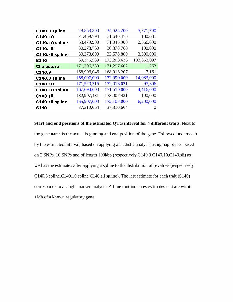
Start and end positions of the estimated QTG interval for 4 different traits. Next to

the gene name is the actual beginning and end position of the gene. Followed underneath

by the estimated interval, based on applying a cladistic analysis using haplotypes based

on 3 SNPs, 10 SNPs and of length 100kbp (respectively C140.3,C140.10,C140.sli) as

well as the estimates after applying a spline to the distribution of p-values (respectively

C140.3 spline,C140.10 spline,C140.sli spline). The last estimate for each trait (S140)

corresponds to a single marker analysis. A blue font indicates estimates that are within

1Mb of a known regulatory gene.

FIGURE LEGENDS

FIGURE 1A:

Comparison between the 20k map (top) versus 140k map (bottom). Points represent

the association between the albinism phenotype and individual SNPs. Colours represent

different chromosomes. Tyrosinase is located on chromosome 7.

FIGURE 1B:

Comparison between the 20k map (top) versus 140k map (bottom). Points represent

the association between the albinism phenotype and haplotypes of length 3 using cladistic

analysis. Colours represent different chromosomes. Tyrosinase is located on chromosome

7.

FIGURE 2A:

Comparison between the 20k map (top) versus 140k map (bottom). Points represent

the association between the albinism phenotype and individual SNPs along chromosome

7. The position of the tyrosinase gene is represented by a red bar.

FIGURE 2B:

Comparison between the 20k map (top) versus 140k map (bottom). Points represent

the association between the albinism phenotype and haplotypes of length 3 using cladistic

analysis along chromosome 7. The position of the tyrosinase gene is represented by a red

bar.

FIGURE 3A:

Comparison between the 20k map (top) versus 140k map (bottom). Points represent

the association between the blindness phenotype and individual SNPs along chromosome

5. The position of the pde6b gene is represented by a red bar.

FIGURE 3B:

Comparison between the 20k map (top) versus 140k map (bottom). Points represent

the association between the blindness phenotype and haplotypes of length 3 using

cladistic analysis along chromosome 5. The position of the pde6b gene is represented by

a red bar.

FIGURE 4:

Cladistic analysis based on a 10 SNP haplotype. Similar haplotypes get merged into

groups and a test for association is performed at each level of the tree. Missing data are

allowed as illustrated here, <NA> get assigned to the most likely group.

FIGURE 5:

Comparison between the different algorithms in estimating gene position in a

mendelian trait. Starting from the top: P-value distribution using a single marker

analysis (S140), cladistic analysis with 3 SNP haplotype (C140.3), cladistic analysis with

a 10 SNP haplotype (C140.10), cladistic analysis of length 100kb (C140.sli), C140.3 after

applying a smoother, C140.10 after applying a smoother and C140.sli after applying a

smoother. X-axis represents the bp position along chromosome 7, the underlying gene for

albinism, tyrosinase, is situated at 74.5Mb.

FIGURE 6:

Comparison between the different algorithms in estimating gene position in a

complex trait. Starting from the top: P-value distribution using a single marker analysis

(S140), cladistic analysis with 3 SNP haplotype (C140.3), cladistic analysis with a 10

SNP haplotype (C140.10), cladistic analysis of length 100kb (C140.sli), C140.3 after

applying a smoother, C140.10 after applying a smoother and C140.sli after applying a

smoother. X-axis represents the bp position along chromosome 1, one contributing gene

for cholesterol, ApoA2, is situated at 171.3Mb and is represented by a vertical line.

FIGURE 7:

An integrated strategy to narrowing down the genome to a list of candidate genes.

Integrated work flow brings in information from linkage analysis, IBD blocks, in silico

analysis and gene expression to get to a short list of candidate genes. This example is

based on the cholesterol trait.

FIGURES

FIGURE 1A:

FIGURE 1B:

FIGURE 2A:

FIGURE 2B:

FIGURE 3A:

FIGURE 3B:

FIGURE 4:

FIGURE 5:

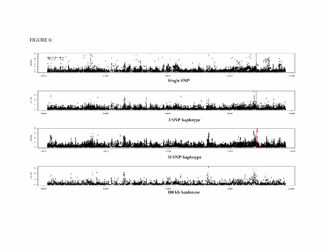
FIGURE 6:

FIGURE 7: