An integrated pan‐tropical biomass map using multiple … · 2015-10-29 · Accepted Article This article has been accepted for publication and undergone full peer review but has

Acc

epte

d A

rtic

le

This article has been accepted for publication and undergone full peer review but has not been through the copyediting, typesetting, pagination and proofreading process, which may lead to differences between this version and the Version of Record. Please cite this article as doi: 10.1111/gcb.13139 This article is protected by copyright. All rights reserved.

Received Date : 09-Jul-2015 Revised Date : 23-Sep-2015 Accepted Date : 24-Sep-2015 Article type : Primary Research Articles An integrated pan-tropical biomass map using multiple reference datasets

(PAN-TROPICAL FUSED BIOMASS MAP)

Avitabile V. 1, Herold M. 1, Heuvelink G.B.M. 1, Lewis S.L. 2,3, Phillips O.L. 2, Asner G.P. 4,

Armston J. 5,6, Asthon P.7,8, Banin L.F.9, Bayol N. 10, Berry N.11, Boeckx P.12, de Jong B. 13,

DeVries B. 1, Girardin C. 14, Kearsley E. 12,15, Lindsell J.A. 16, Lopez-Gonzalez G. 2, Lucas R.

17, Malhi Y. 14, Morel A. 14, Mitchard E. 11, Nagy L. 18, Qie L.2, Quinones M. 19, Ryan C.M. 11,

Slik F. 20, Sunderland, T. 21, Vaglio Laurin G. 22, Valentini R. 23, Verbeeck H. 12, Wijaya A. 21,

Willcock S. 24

1. Wageningen University, the Netherlands; 2. University of Leeds, UK; 3. University

College London, UK; 4. Carnegie Institution for Science, USA; 5. The University of

Queensland, Australia; 6. Information Technology and Innovation, Australia; 7. Harvard

University, UK; 8. Royal Botanic Gardens, UK; 9. Centre for Ecology and Hydrology, UK;

10. Foret Ressources Management, France; 11. University of Edinburgh, UK; 12. Ghent

University, Belgium; 13. Ecosur, Mexico; 14. University of Oxford, UK; 15. Royal Museum

for Central Africa, Belgium; 16. The RSPB Centre for Conservation Science, UK; 17. The

University of New South Wales, Australia; 18. Universidade Estadual de Campinas, Brazil;

19. SarVision, the Netherlands; 20. Universiti Brunei Darussalam, Brunei; 21. Center for

International Forestry Research, Indonesia; 22. Centro Euro-Mediterraneo sui Cambiamenti

Climatici, Italy; 23. Tuscia University, Italy; 24. University of Southampton, UK

Acc

epte

d A

rtic

le

This article is protected by copyright. All rights reserved.

Correspondence: Valerio Avitabile, tel. +31 317482092, email: [email protected]

Keywords: aboveground biomass, carbon cycle, forest plots, tropical forest, forest inventory,

REDD+, satellite mapping, remote sensing

Type of paper: Primary Research Article

Abstract

We combined two existing datasets of vegetation aboveground biomass (AGB) (Saatchi et al.,

2011; Baccini et al., 2012) into a pan-tropical AGB map at 1-km resolution using an

independent reference dataset of field observations and locally-calibrated high-resolution

biomass maps, harmonized and upscaled to 14,477 1-km AGB estimates. Our data fusion

approach uses bias removal and weighted linear averaging that incorporates and spatializes

the biomass patterns indicated by the reference data. The method was applied independently

in areas (strata) with homogeneous error patterns of the input (Saatchi and Baccini) maps,

which were estimated from the reference data and additional covariates. Based on the fused

map, we estimated AGB stock for the tropics (23.4 N – 23.4 S) of 375 Pg dry mass, 9% -

18% lower than the Saatchi and Baccini estimates. The fused map also showed differing

spatial patterns of AGB over large areas, with higher AGB density in the dense forest areas in

the Congo basin, Eastern Amazon and South-East Asia, and lower values in Central America

and in most dry vegetation areas of Africa than either of the input maps. The validation

exercise, based on 2,118 estimates from the reference dataset not used in the fusion process,

showed that the fused map had a RMSE 15 – 21% lower than that of the input maps and,

most importantly, nearly unbiased estimates (mean bias 5 Mg dry mass ha-1 vs. 21 and 28 Mg

ha-1 for the input maps). The fusion method can be applied at any scale including the policy-

relevant national level, where it can provide improved biomass estimates by integrating

Acc

epte

d A

rtic

le


existing regional biomass maps as input maps and additional, country-specific reference

datasets.

Introduction

Recently, considerable efforts have been made to better quantify the amounts and spatial

distribution of aboveground biomass (AGB), a key parameter for estimating carbon emissions

and removals due to land-use change, and related impacts on climate (Saatchi et al., 2011;

Baccini et al., 2012; Harris et al., 2012; Houghton et al., 2012; Mitchard et al., 2014; Achard

et al., 2014). Particular attention has been given to the tropical regions, where uncertainties

are higher (Pan et al., 2011; Ziegler et al., 2012; Grace et al., 2014). In addition to ground

observations acquired by research networks or for forest inventory purposes, several AGB

maps have been recently produced at different scales, using a variety of empirical modelling

approaches based on remote sensing data calibrated by field observations (e.g., Goetz et al.,

2011; Birdsey et al., 2013). AGB maps at moderate resolution have been produced for the

entire tropical belt by integrating various satellite observations (Saatchi et al., 2011; Baccini

et al., 2012), while higher resolution datasets have been produced at local or national level

using medium-high resolution satellite data (e.g., Avitabile et al., 2012; Cartus et al., 2014),

sometimes in combination with airborne Light Detection and Ranging (LiDAR) data (Asner

et al., 2012a, 2012b, 2013, 2014a). The various datasets often have different purposes:

research plots provide a detailed and accurate estimation of AGB (and other ecological

parameters or processes) at the local level, forest inventory networks use a sampling approach

to obtain statistics of biomass stocks (or growing stock volume) per forest type at the sub-

national or national level, while high-resolution biomass maps can provide detailed and

spatially explicit estimates of AGB density to assist natural resource management, and large

Acc

epte

d A

rtic

le


scale coarse-resolution datasets depict AGB distribution for global-scale carbon accounting

and modelling.

In the context of the United Nations mechanism for Reducing Emissions from Deforestation

and forest Degradation (REDD+), emission estimates obtained from spatially explicit

biomass datasets may be favoured over those based on mean values derived from plot

networks. This preference stems from the fact that plot networks are not designed to represent

land cover change events, which usually do not occur randomly and may affect forests with

biomass density systematically different from the mean value (Baccini and Asner, 2013).

With very few tropical countries having national AGB maps or reliable statistics on forest

carbon stocks, regional maps may provide advantages compared to the use of default mean

values (e.g., IPCC (2006) Tier 1 values) to assess emissions from deforestation, as long as

their accuracy is reasonable and their estimates are not affected by systematic errors

(Avitabile et al., 2011). These conditions are difficult to assess, however, since rigorous

validation of regional AGB maps remains problematic, given their large area coverage and

large mapping unit (Mitchard et al., 2013), while ground observations are only available for a

limited number of small sample areas.

The comparison of two recent pan-tropical AGB maps (Saatchi et al., 2011; Baccini et al.,

2012) revealed substantial differences between the two products (Mitchard et al., 2013).

Further comparison with ground observations and high-resolution maps also highlighted

notable differences in AGB patterns at regional scales (Baccini and Asner, 2013; Hills et al.,

2013; Mitchard et al., 2014). Such comparisons have stimulated a debate over the use and

capabilities of different types of biomass products (Saatchi et al., 2014; Langner et al., 2014)

and have highlighted both the importance and sometimes the lack of integration of different

Acc

epte

d A

rtic

le


datasets. On one hand, the two pan-tropical maps are consistent in terms of methodology

because both use the same primary data source (GLAS LiDAR) alongside a similar

modelling approach to upscale the LiDAR data to larger scales. Moreover, they have the

advantage of being calibrated using hundreds of thousands of AGB estimates derived from

height metrics computed by a spaceborne LiDAR sensor distributed over the tropics.

However, such maps are based on remotely sensed variables that do not directly measure

AGB, but are sensitive to canopy cover and canopy height parameters that do not fully

capture the AGB variability of complex tropical forests. Furthermore, both products assume

global or continental allometric relationships in which AGB varies only with stand height,

and further errors are introduced by upscaling the calibration data to the coarser satellite data.

On the other hand, ground plots use allometric equations to estimate AGB at individual tree

level using directly measurable parameters such as diameter, height and species identity

(hence wood density). However, they have limited coverage, are not error-free, and

compiling various datasets over large areas is made more complex due to differing sampling

strategies (e.g., stratification of landscapes, plot size, minimum diameter of trees measured).

Considering the rapid increase of biomass observations at different scales and the different

capabilities and limitations of the various datasets, it is becoming more and more important to

identify strategies that are capable of making best use of existing information and optimally

integrate various data sources for improved large area AGB assessment (e.g., see Willcock et

al., 2012).

In the present study, we compiled existing ground observations and locally-calibrated high-

resolution biomass maps to obtain a high-quality AGB reference dataset for the tropical

region (Objective 1). This reference dataset was used to assess two existing pan-tropical AGB

maps (Objective 2) and to combine them in a fused map that optimally integrates the two

Acc

epte

d A

rtic

le


maps, based on the method presented by Ge et al. (2014) (Objective 3). Lastly, the fused map

was assessed and compared to known AGB stocks and patterns across the tropics (Objective

4).

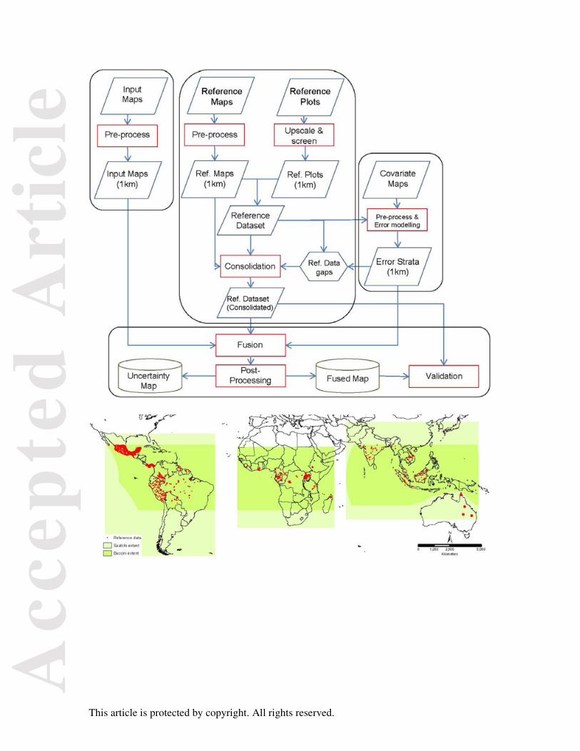
Overall, the approach consisted of pre-processing, screening and harmonizing the pan-

tropical AGB maps (called ‘input maps’), the high-resolution AGB maps (called ‘reference

maps’) and the field plots (called ‘reference plots’; ‘reference dataset’ refers to the maps and

plots combined) to a common spatial resolution and geospatial reference system (Figure 1).

The input maps were combined using bias removal and weighted linear averaging (‘fusion’).

The fusion model was applied independently to areas associated with different error patterns

of the input maps (called ‘error strata’), which were estimated from the reference data and

additional covariates (called ‘covariate maps’). The reference dataset included only a subset

of the reference maps (i.e., the cells with highest confidence) and if a stratum was lacking

reference data (‘reference data gaps’), additional data were extracted from the reference maps

(‘consolidation’). The fused map was validated using independent data and its uncertainty

quantified using model parameters. In this study, the terms AGB refers to aboveground live

woody biomass and is reported in units of Mg dry mass ha-1. The fused map and the

corresponding reference dataset can be freely downloaded from

www.wageningenur.nl/grsbiomass.

Materials and methods

Input maps

The input maps used for this study were the two pan-tropical datasets published by Saatchi et

al. (2011) and Baccini et al. (2012), hereafter referred to as the “Saatchi” and “Baccini” maps

individually, or as “input” maps collectively. The Baccini map was provided in MODIS

Acc

epte

d A

rtic

le


sinusoidal projection with a spatial resolution of 463 m while the Saatchi map was in a

geographic projection (WGS-84) at 0.00833 degrees (approximately 1 km) pixel size. The

two datasets were harmonized by first projecting the Baccini map to the coordinate system of

the Saatchi map using the Geospatial Data Abstraction Library (www.gdal.org) and then

aggregating it to match the spatial resolution and grid of the Saatchi map. Spatial aggregation

was performed by computing the mean value of the pixels whose centre was located within

each 1-km cell of the Saatchi map. Resampling was then undertaken using the nearest

neighbor method.

Reference dataset

The reference dataset comprised individual tree-based field data and high-resolution AGB

maps independent from the input maps. The field data included AGB estimates derived from

field measurement of tree parameters and allometric equations. The AGB maps included

high-resolution (≤ 100 m) datasets derived from satellite data using empirical models

calibrated and validated using local ground observations and, in some cases, airborne LiDAR

measurements. Given the variability of procedures used to acquire and produce the various

datasets, they were first screened according to a set of quality criteria to select only the most

reliable AGB estimates, and then pre-processed to be harmonized with the pan-tropical AGB

maps in terms of spatial resolution and observed variables. Field and map datasets providing

aboveground carbon density were converted to AGB units using the same coefficients used

for their original conversion from biomass to carbon. The sources and characteristics of the

reference data are listed in the Supplementary Information (Tables S8 - S11).

Acc

epte

d A

rtic

le


Data screening and pre-processing

Reference field data

The reference field data were measurements from forest inventory plots for which accurate

geolocation and biomass estimates were available. Pre-processing of the data consisted of a

2-step screening and a harmonization procedure. A preliminary screening selected only the

ground data that satisfied the following criteria: (1) they estimated AGB for all living trees

with diameter at breast height ≥ 5-10 cm; (2) they were acquired on or after the year 2000; (3)

they were not used to calibrate the LiDAR-AGB relationships of the input maps; and (4) their

plot coordinates were measured using a GPS. Since the taxonomic identities of trees strongly

indicate wood density, and hence stand-level biomass (e.g., Baker et al., 2004; Mitchard et al.

2014), plots were only selected if tree AGB was estimated using at least tree diameter and

wood density as input parameters. Datasets were excluded if they did not conform to these

requirements or did not provide clear information on the biomass pool measured, the tree

parameters measured in the field, the allometric model applied, the year of measurement or

the plot geolocation and extent. Next, the plot data were projected to the geographic reference

system WGS-84 and harmonized with the input maps by averaging the AGB values located

within the same 1-km pixel if there was more than one plot per pixel, or by directly

attributing the plot AGB to the respective pixel if there was only one plot per pixel. Field

plots not fully located within one pixel were attributed to the map cell where the majority of

the plot area (i.e., the plot centroid) was located.

Lastly, the representativeness of the plot over the 1-km pixels was considered, and the ground

data were further screened to discard plots not representative of the map cells in terms of

AGB density. More specifically, since the two input maps in their native reference systems

are not aligned and therefore their pixels do not correspond to the same geographic area, the

Acc

epte

d A

rtic

le


plot representativeness was assessed on the area of both pixels (identified before the map

resampling). The representativeness was evaluated on the basis of the homogeneity of the tree

cover and crown size within the pixel, determined through visual interpretation of high-

resolution images provided on the Google Earth platform. If the tree cover and tree crowns

were not homogeneous over at least 90% of the pixel area, the plots located within the pixel

were discarded (Fig. S1). In addition, if subsequent Google Earth images indicated that forest

change processes (e.g., deforestation or regrowth) occurred in the period between the field

measurement and the reference years of the input maps, the corresponding plots were

discarded.

Reference biomass maps

The reference biomass maps consisted of high-resolution local or national AGB maps

published in the scientific literature. Maps providing AGB estimates grouped in classes (e.g.,

Willcock et al., 2012) were not used since the class values represent the mean AGB over

large areas, usually spanning multiple strata used in the present study (see ‘Stratification

approach’). The reference AGB maps were first pre-processed to match the input maps

through re-projection, aggregation and resampling using the same procedures described for

the pre-processing of the Baccini map. Then, only the cells with largest confidence (i.e.,

lowest uncertainty) were selected from the maps. Since uncertainty maps were usually not

available, and considering that the reference maps were based on empirical models, the map

cells with greatest confidence were assumed to be those in correspondence of the training

data (field plots and/or LiDAR data). When the locations of the training data were not

available, random pixels were extracted from the maps. For maps based only on radar or

optical data, whose signals saturate above a certain AGB density value, only pixels below

such a threshold were considered. In order to compile a reference database that was

Acc

epte

d A

rtic

le


representative of the area of interest and well-balanced among the various input datasets (as

defined in ‘Consolidation of the reference dataset’), the amount of reference data extracted

from the AGB maps was proportional to their area and not greater than the amount of

samples provided by the field datasets representing a similar area. In the case where maps

with extensive training areas provided a disproportionate number of reference pixels, a

further screening selected only the areas underpinned by the largest amount of training data.

Consolidation of the reference dataset

Considering that the modelling approach used in this study is applied independently by

stratum (which represent areas with homogeneous error structure in both input maps; see

‘Stratification approach’) and is sensitive to the characteristics of the reference data (see

‘Modelling approach’), each stratum requires that calibration data are relatively well-

balanced between the various reference datasets. Specifically, if a stratum contains few

calibration data, the model becomes more sensitive to outliers, while if a reference dataset is

much larger than the others, the model is more strongly determined by the dominant dataset.

For these reasons, for the strata where the reference dataset was under-represented or un-

balanced, it was consolidated by additional reference data taken from the reference AGB

maps, if available. The reference data were considered insufficient if a stratum had less than

half of the average reference data per stratum, and were considered un-balanced if a single

dataset provided more than 75% of the reference data of the whole stratum and it was not

representative of more than 75% of its area. In such cases, additional reference data were

randomly extracted from the reference AGB maps that did not provide more than 75% of the

reference data. The amount of data to be extracted from each map was computed in a way to

obtain a reference dataset with an average number of reference data per stratum and not

dominated by a single dataset. If necessary, additional training data representing areas with

Acc

epte

d A

rtic

le


no AGB (e.g., bare soil) were included, using visual analysis of Google Earth images to

identify locations without vegetation.

Selected reference data

The AGB reference dataset compiled for this study consisted of 14,477 1-km reference pixels,

distributed as follows: 953 in Africa, 449 in South America, 7,675 in Central America, 400 in

Asia and 5,000 in Australia (Fig. 2, Table 1). The reference data were relatively uniformly

distributed among the strata (Table S6) but their amount varied considerably by continent.

The average amount of reference data per stratum ranged from 50 (Asia) to 958 (Central

America) 1-km reference pixels and their variability (computed as standard deviation relative

to the mean) ranged from 25% (South America) to 52% (Central America). The uneven

distribution of reference data across the continents is mostly caused by the availability of

ground observations: as indicated above, in order to have a balanced reference dataset for

each stratum the reference data extracted from AGB maps were limited to the (smaller)

amount of direct field observations. When AGB maps were the only source of data, this

constraint was not occurring and larger datasets could be derived from the maps (i.e., Central

America, Australia).

The reference data were selected from 18 ground datasets and from 9 high-resolution AGB

maps calibrated by field observations and, in 4 cases, airborne LiDAR data (Table 1). The

field plots used for the calibration of the maps are not included in this section because they

were only used to select the reference pixels from the maps. The visual screening of the field

plots removed 35% of the input data (from 6,627 to 4,283) and their aggregation to 1-km

resolution further removed 70% of the reference units derived from field plots (from 4,283 to

1,274), while 10,741 reference pixels were extracted from the high-resolution AGB maps.

Acc

epte

d A

rtic

le


The criteria used to select the reference pixels for each map are reported in Table S2. The

consolidation procedure was necessary only for Central America where it added 2,415

reference data, while 47 pixels representing areas with no AGB were identified in Asia

(Table S1). In general, ground observations were mostly discarded in areas characterized by

fragmented or heterogeneous vegetation cover and high biomass spatial variability. In such

contexts, reference data were often acquired from the AGB maps.

Stratification approach

Preliminary comparison of the reference data with the input maps showed that the error

variances and biases of the input maps were not spatially homogeneous but varied

considerably in different regions. Since the fusion model used in this study (see ‘Modelling

approach’) is based on bias removal and weighted combination of the input maps, the more

homogeneous the error characteristics in the input maps are, the better they can be reduced by

the model. For this reason, the stratification approach aimed at identifying areas with

homogeneous error structure (hereafter named ‘error strata’) in both input maps. A first

stratification was undertaken based on geographic location (namely Central America, South

America, Africa, Asia and Australia) to reflect the regional allometric relationships between

AGB and tree diameter and height (Feldpausch et al., 2011, 2012). Then, the error strata were

identified for each continent using a two-step process. First, the error maps of the Saatchi and

Baccini maps were predicted separately. Since the AGB estimates of the input maps were

mostly based on optical and LiDAR data that are sensitive to tree cover and tree height, it was

assumed that their uncertainties were related to the spatial variation of these parameters. In

addition, the errors of the input maps were found to be linearly correlated with the respective

AGB estimates. For these reasons, the AGB maps themselves, as well as global datasets of

land cover (ESA, 2014a), tree cover (Di Miceli et al., 2014) and tree height (Simard et al.,

Acc

epte

d A

rtic

le


2011), were used to predict the map errors using a Random Forest model (Breiman, 2001)

calibrated on the basis of the reference dataset. Second, the error maps of the Saatchi and

Baccini datasets were clustered using the K-Means approach. The use of eight clusters (hence,

eight error strata) was considered a sensible trade-off between homogeneity of the errors of

the input maps and number of reference observations available per stratum, with a larger

number of clusters providing only a marginal increase in homogeneity but leading to a small

number of reference data in some strata (Fig. S2). In areas where the predictors presented no

data (i.e., outside the coverage of the Baccini map) or for classes of the categorical predictor

without reference data (i.e., land cover), the error strata (instead of the error maps) were

predicted using an additional Random Forest model based on predictors without missing

values (i.e., Saatchi map, tree cover and tree height) and 10,000 training data randomly

extracted from the stratification map.

This method produced a stratification map that identified eight strata for each continent with

homogeneous error patterns in the input maps (Fig. S3). The root mean square error (RMSE)

computed on the Out-Of-Bag data (i.e., data not used for training) of the Random Forest

models that predicted the errors of the input maps ranged between 22.8 ± 0.3 Mg ha-1

(Central America) to 83.7 ± 2.5 Mg ha-1 (Africa), with the two models (one for each input

map) achieving similar accuracies in each continent (Table S4, Fig. S4). In most cases the

main predictors of the errors of the input maps were the biomass values of the maps

themselves, followed by tree cover and tree height, while land cover was always the least

important predictor (Table S5). Further details on the processing of the input data are

provided in the Supplementary Information.

Acc

epte

d A

rtic

le


The use of a stratification based on the errors of the input maps was compared with

stratifications based on land cover (used by Ge et al., 2014), tree cover and tree height. A

separate stratification map was obtained for each of these alternative variables by aggregation

into eight strata (to maintain comparability with the number of clusters used in the error

strata), and each stratification map was used to develop a specific fused map. The

performance of alternative stratification approaches was assessed by validating the respective

fused maps (see Supplementary Information – Alternative stratification approaches). The

results demonstrated that the stratification based on error modelling and clustering (i.e., the

error strata) produced a fused map with higher accuracy than that of the maps based on other

stratification approaches, and therefore was used in this study (Fig. S5).

Modelling approach

The fusion model

The integration of the two input maps was performed with a fusion model based on the

concept presented by Ge et al. (2014) and further developed for this study. The fusion model

consists of bias removal and weighted linear averaging of the input maps to produce an

output with greater accuracy than each of the input maps. The reference AGB dataset

described above was used to calibrate the model and to assess the accuracy of the input and

fused maps. A specific model was developed for each stratum.

Following Ge et al. (2014), the p input maps for locations s∈D, where D is the geographical

domain of interest common to the input maps, were combined using a weighted linear

average:

(1) 1

( ) ( ) ( ( ) ( ))=

= ⋅ − p

i i iif s w s z s v s

Acc

epte

d A

rtic

le


where f is the fused map, the wi(s) are weights, zi the estimate of the i-th input map and vi(s)

is the bias estimate. The bias term was computed as the average difference between the input

map and the reference data for each stratum. The weights were obtained from a statistical

model that assumes the map estimates zi to be the sum of the true biomass bi with a bias term

vi and a random noise term εi with zero mean for each location s∈D. We further assumed that

the εi of the input maps are jointly normally distributed with variance-covariance matrix C(s).

Differently from Ge et al. (2014), C(s) was estimated using a robust covariance estimator as

implemented by the ‘robust’ package in R (Wang et al., 2014), which uses the Stahel-Donoho

estimator for strata with fewer than 5,000 observations and the Fast Minimum Covariance

Determinant estimator for larger strata. Under these assumptions, the variance of the

estimation error of the fused map f(s) is minimized by calculating the weights w(s) as

outlined by Searle (1971, p. 89):

(2) ( ) 11 1( ) ( ) ( )−− −= 1 C 1 1 CT T Tw s s s

where 1=[1, ..., 1]T is the transpose of the p-dimensional unit vector. The weights computed

for each stratum sum to 1, while their values are approximately inversely proportional to the

error variance of the corresponding input map. Larger weights are assigned to input maps

with lower error variances, although the covariance between map errors influences the

weights as well. Overall, the fused map is expected to provide more accurate estimates after

bias removal and weighted averaging of the input maps. The fusion model assured that the

variance of the error in the fused map was smaller than that of the input maps (Bates and

Granger, 1969), especially if the errors associated with these maps were not strongly

positively correlated and their error variances were close to the smallest error variance. The

fusion model can be applied to any number of input maps. Where there is only one input map,

the model estimates and removes its bias and the weights are set equal to 1.

Acc

epte

d A

rtic

le


The model parameters

The fusion model computed a set of bias and weight parameters for each stratum and

continent on the basis of their respective reference data, and used these for the linear

weighted combination of the input maps (Table S6). Since the stratification approach grouped

together data with similar error patterns, the biases varied considerably among the strata and

could reach values up to ±200 Mg ha-1. However, considering the area of the strata, the biases

of both input maps were smaller than ±45 Mg ha-1 for at least 50% of the area of all

continents and smaller than ±100 Mg ha-1 for 81% - 98% of the area of all continents.

Post-processing

Predictions outside the coverage of the Baccini map

The Baccini map covers the tropical belt between 23.4 degree north latitude and 23.4 degree

south latitude while the Saatchi map presents a larger latitudinal coverage (Fig. 2). The fusion

model was first applied to the area common to both input maps (Baccini extent) and then

extended to the area where only the Saatchi map is available. In the latter area, the model

focused only on removing the bias of the Saatchi map using the values estimated for the

Baccini extent. The model predictions for the Saatchi extent were mosaicked to those for the

Baccini extent using a smoothing function (inverse distance weight) on an overlapping area

of 1 degree within the Baccini extent between the two maps. Water bodies were masked over

the whole study area using the ESA CCI Water Bodies map (ESA, 2014b). The resulting

fused map was projected to an equal area reference system (MODIS Sinusoidal) before

computing the total AGB stocks for each continent, which were obtained by summing the

products of the AGB density of each pixel with their area.

Acc

epte

d A

rtic

le


Assessing AGB in intact and non-intact forest

The AGB estimates of the fused and input maps in forest areas were further investigated

regarding their distribution in ecozones and between intact and non-intact landscapes. Forest

areas were defined as areas dominated by tree cover according to the GLC2000 map

(Bartholomé and Belward, 2005). Ecozones were defined according to the Global Ecological

Zone (GEZ) map for the year 2000 (FAO, 2000). The intact landscapes were defined

according to the Intact Forest Landscape (IFL) map for the year 2000 (Potapov et al., 2008).

On the basis of these datasets, the mean forest AGB density of the fused and input maps were

computed for intact and non-intact landscapes for each continent and major ecozone. To

allow direct comparison of the results among the maps, the analysis was performed only for

the area common to all maps (Baccini extent). In addition, to reduce the impact of spatial

inaccuracies in the maps, only ecozones with IFL intact forest areas larger than 1,000 km2

were considered. The mean AGB density of intact and non-intact forests per continent was

computed as the area-weighted mean of the contributing ecozones.

Validation and uncertainty

Validation of the fused and input maps was performed by randomly splitting the reference

data into a calibration set (70% of the data) and a validation set (remaining 30%). The ‘final’

fused map presented in Fig. 3 used 100% of the reference data while for validation purposes a

‘test’ fused map was produced using only the calibration data. The estimates of the ‘test’

fused map, as well as those of the input maps, were compared with the validation data. Note

that validation of the ‘test’ fused map only yields an approximate (i.e., conservative) estimate

of the accuracy of the ‘final’ fused map. In other words, the ‘final’ fused map is likely more

accurate than the ‘test’ fused map because it uses a larger calibration data set. To maintain

full independence, validation data were not used for any step related to the development of

Acc

epte

d A

rtic

le


the ‘test’ fused map, including production of the stratification map. To account for any

potential impacts of the random selection of validation data, the procedure was repeated 100

times, computing a new random selection of the calibration and validation datasets with each

iteration. This procedure allowed computing the mean RMSE and assessing its standard

deviation for the fused and input maps.

The uncertainty of the fused map was computed with respect to model uncertainty, not

including the error sources in the input data (see ‘Discussion’). The model uncertainty

consisted of the expected variance of the error of the fused map (which is assumed to be bias-

free) and was derived for each stratum from C(s). The uncertainty was thus estimated per

strata and not at the pixel level. The error variance was converted to an uncertainty map by

reclassifying the stratification map, where the stratum value was converted to the respective

error variance computed for each stratum and continent.

Results

Biomass map

The fusion model produced an AGB map at 1-km resolution for the tropical region, with an

extent equal to that of the Saatchi map (Fig. 3). In terms of stocks, the AGB estimates within

the fused map were lower than both input maps at continental level. The total stock of the

fused map for the tropical belt covered by the Baccini map (23.4 N – 23.4 S, see Fig. 2) was

375 Pg dry mass, 9% and 18% lower than the Saatchi (413 Pg) and Baccini (457 Pg)

estimates, respectively. Considering the larger extent of the Saatchi map, the fused map

estimate was 462 Pg, 15% lower than the estimate of the Saatchi map (545 Pg) (Table S7).

Acc

epte

d A

rtic

le


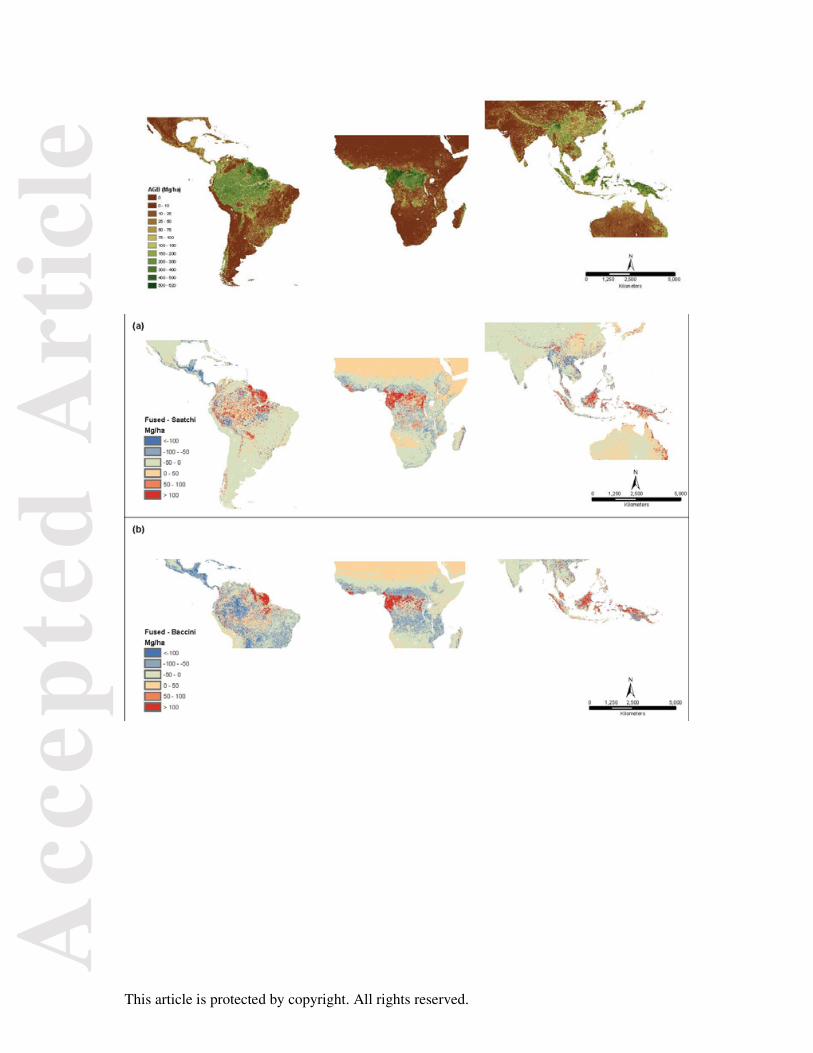
Moreover, the fused map presented spatial patterns that differed substantially from both input

maps (Fig. 4): the AGB estimates were higher than the Saatchi and Baccini maps in the dense

forest areas in the Congo basin, in West Africa, in the north-eastern part of the Amazon basin

(Guyana shield) and in South-East Asia, and lower in Central America and in most dry

vegetation areas of Africa. In the central part of the Amazon basin the fused map showed

lower estimates than the Baccini map and higher estimates than the Saatchi map, while in the

southern part of the Amazon basin these differences were inversed. Similar trends emerged

when comparing the maps separately for intact and non-intact forest ecozones (Supporting

Information). In addition, the average difference between intact and non-intact forests was

larger than that derived from the input maps in Africa and Asia, similar or slightly larger in

South America, and smaller in Central America (Fig. S6).

According to the fused map, the highest AGB density (> 400 Mg ha-1) is found in the Guyana

shield, in the central and western part of the Congo basin and in the intact forest areas of

Borneo and Papua New Guinea. The analysis of the distribution of forest AGB in intact and

non-intact ecozones showed that the mean AGB density was greatest in intact African (360

Mg ha-1) and Asian (335 Mg ha-1) forests, followed by intact forests in South America (266

Mg ha-1) and Central America (146 Mg ha-1) (Fig. S6). AGB in non-intact forests was much

lower in all regions (Africa, 78 Mg ha-1; Asia, 211 Mg ha-1; South America, 149 Mg ha-1; and

Central America, 57 Mg ha-1) (Fig. S6).

Validation

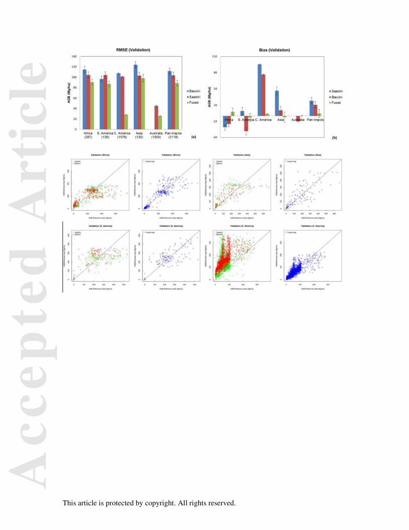
The validation exercise showed that the fused map achieved a lower RMSE (a decrease of 5 –

74%) and bias (a decrease of 90 – 153%) than the input maps for all continents (Fig. 5).

While the RMSE of the fused map was consistently lower than that of the input maps but still

Acc

epte

d A

rtic

le


substantial (87 – 98 Mg ha-1) in the largest continents (Africa, South America and Asia), the

mean error (bias) of the fused map was almost null in most cases. Moreover, in the three

main continents the bias of the input maps tended to vary with biomass, with overestimation

at low values and underestimation at high values, while the errors of the fused map were

more consistently distributed (Fig. 6). When computing the error statistics for the pan-tropics

(Baccini extent) as the average of the regional validation results weighted by the respective

area coverage, the mean bias (in absolute terms) for the fused, Saatchi and Baccini maps was

5, 21 and 28 Mg ha-1 and the mean RMSE was 89, 104 and 112 Mg ha-1, respectively (Fig. 5).

The accuracy of the input maps reported above was computed using the validation dataset

(30% of the reference dataset) to be consistent with the accuracy of the fused map. The

accuracy of the input maps was also computed using all reference data and the results (Table

S3) were similar to those based on the validation dataset.

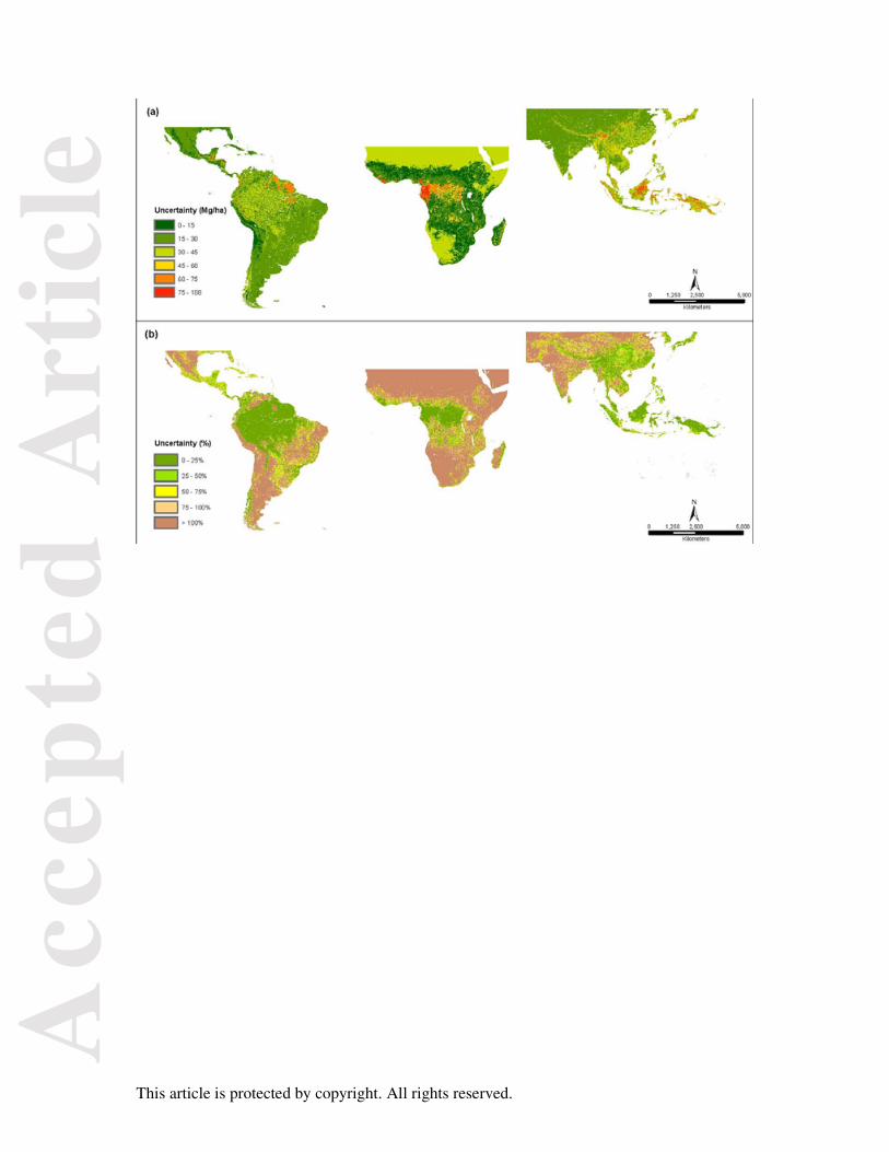
Uncertainty map

The uncertainty of the model predictions indicated that the standard deviation of the error of

the fused map for each stratum was in the range 11 - 108 Mg ha-1, with largest uncertainties

in areas with largest AGB estimates (Congo basin, Eastern Amazon basin and Borneo). When

computed in relative terms (as a percentage of the AGB estimate), the model uncertainties

presented opposite patterns, with uncertainties larger than the estimates (> 100%) in the low

AGB areas (< 20 Mg ha-1 on average) of Africa, South America and Central America, while

high AGB forests (> 210 Mg ha-1 on average) had uncertainties lower than 25% (Fig. 7). The

uncertainty measure derived from C(s) was computed only when two or more input maps

were available. Hence, it could not be calculated for Australia because the model for this

continent was based on only one input map (Saatchi map).

Acc

epte

d A

rtic

le


Discussion

Biomass patterns and stocks emerging from the reference data

The AGB map produced with the fusion approach is largely driven by the reference dataset

and essentially the method is aimed at spatializing the AGB patterns indicated by the

reference data using the support of the input maps. For this reason, great care was taken in the

pre-processing of the reference data, which included a two-step quality screening based on

metadata analysis and visual interpretation, and their consolidation after stratification. As a

result, the reference dataset provides an unprecedented compilation of AGB estimates at 1-

km resolution for the tropical region, covering a wide range of vegetation types, biomass

ranges and ecological regions across the tropics. It includes the most comprehensive and

accurate tropical field plot networks and high-quality maps calibrated with airborne LiDAR,

which provide more accurate estimates compared to those obtained from other sensors

(Zolkos et al., 2013). The main trends present in the fused map emerged from the

combination of different and independent reference datasets and are in agreement with the

estimates derived from long-term research plot networks (Malhi et al., 2006; Phillips et al.,

2009; Lewis et al., 2009; Slik et al., 2010, 2013; Lewis et al., 2013) and high-resolution maps

(Asner et al., 2012a, 2012b, 2013, 2014a). Specifically, the AGB patterns in South America

represent spatial trends described by research plot networks in the dense intact and non-intact

forests in the Amazon basin, forest inventory plots collected in the dense forests of Guyana

and samples extracted from AGB maps for Colombia and Peru representing a wide range of

vegetation types, from arid grasslands to humid forests. Similarly, AGB patterns depicted in

Africa were derived from a combination of various research plots in dense undisturbed forest

(Gabon, Cameroon, Democratic Republic of Congo, Ghana, Liberia), inventory plots in forest

concessions (Democratic Republic of Congo), AGB maps in woodland and savannah

ecosystems (Uganda, Mozambique) and research plots and maps in montane forests (Ethiopia,

Acc

epte

d A

rtic

le


Madagascar). Most vegetation types in Central America, Asia and Australia were also well-

represented by the extensive forest inventory plots (Indonesia, Vietnam and Laos) and high-

resolution maps (Mexico, Panama, Australia).

In spite of the extensive coverage, the current database is far from being representative of the

AGB variability across the tropics. As a consequence, the model estimates are expected to be

less accurate in contexts not adequately represented. In the case of the fusion approach, this

corresponds to the areas where the input maps present error patterns different than those

identified in areas with reference data: in such areas the model parameters used to correct the

input maps (bias and weight) may not adequately reflect the errors of the input maps and

hence cannot optimally correct them. In particular, deciduous vegetation and heavily

disturbed forest of Africa and South America, and large parts of Asia were lacking quality

reference data. Moreover, even though plot data were spatially distributed over the central

Amazon and the Congo basin, large extents of these two main blocks of tropical forest have

never been measured (cf. maps in Lewis et al., 2013; Mitchard et al., 2014). Considering the

evidence of significant local differences in forest structure and AGB density within the same

forest ecosystems (Kearsley et al., 2013), additional data are needed to strengthen the

confidence of the fused map as well as that of any other AGB map covering the tropical

region. Moreover, a dedicated gap analysis to assess the main regions lacking AGB reference

data and identify priority areas for new field sampling and LiDAR campaigns would be very

valuable for future improved biomass mapping.

Regarding the AGB stocks, a previous study showed that despite their often very strong local

differences, the two input maps tended to provide similar estimates of total stocks at national

and biome scales and presented an overall net difference of 10% for the pan-tropics

Acc

epte

d A

rtic

le


(Mitchard et al., 2013). However, such convergence is mostly due to compensation of

contrasting estimates when averaging over large areas. The larger differences with the

estimates of the present study (9% and 18%) suggest an overestimation of the total stocks by

the input maps. This is in agreement with the results of two previous studies that, on the basis

of reference maps obtained by field-calibrated airborne LiDAR data, identified an

overestimation of 23% - 42% of total stocks in the Saatchi and Baccini maps in the

Colombian Amazon (Mitchard et al., 2013) and a mean overestimation of about 100 Mg ha-1

for the Baccini map in the Colombian and Peruvian Amazon (Baccini and Asner, 2013).

In general, the AGB density values of the fused map were calibrated and therefore in

agreement with the existing estimates obtained from plot networks and high-resolution maps.

The comparison of mean AGB values in intact and non-intact forests stratified by ecozone

provided further information on the differences between the maps. The mean AGB values of

the fused map in non-intact forests were mostly lower than those of the input maps,

suggesting that in disturbed forests the AGB estimates derived from stand height parameters

retrieved by spaceborne LiDAR (as in the input maps) tend to be higher compared to those

based on tree parameters or very high-resolution airborne LiDAR measurements (as in the

fused map and reference data). This difference occurred especially in Africa, Asia and

Central America while it was less evident in South America and Australia. By contrast, the

differences among the maps for intact forests varied by continent, with the fused map having,

on average, higher mean AGB values in Africa, Asia and Australia, lower values in Central

America, and variable trends within South America, reflecting the different allometric

relationships used by the various datasets in different continents.

Acc

epte

d A

rtic

le


As mentioned above, a larger amount of reference data, ideally acquired based on a clear

statistical sampling design instead of one that is opportunistic, will be required to confirm

such conclusions. While dense sampling of tropical forests using field observations is often

impractical, new approaches combining sufficient ground observations of individual trees at

calibration plots with airborne LiDAR measurements for larger sampling transects would

allow a major increase in the quantity of calibration data. In combination with wall-to-wall

medium resolution satellite data (e.g., Landsat) these may be capable of achieving high

accuracy over large areas (10% - 20% uncertainty at 1-ha scale) while being cost-effective

(e.g., Asner et al., 2013, 2014b). In addition, new technologies, such as Terrestrial Laser

Scanning (TLS), allows for better estimates at ground level (Calders et al., 2015; Gonzalez de

Tanago et al., 2015), considerably reducing the uncertainties of field estimates based on

generalized allometric equations and avoiding destructive sampling. Nevertheless, since

floristic composition influences AGB at multiple scales (e.g., the strong pan-Amazon

gradient in wood density shown by ter Steege et al., 2006) such techniques benefit from

extensive and precise measurements of tree identity in order to determine wood density

patterns and to account for variations in hollow stems and rottenness (Nogueira et al., 2006).

Moreover, we note that the reference data do not include lianas, which may constitute a

substantial amount of woody stems, and their inclusion would allow to obtain more correct

estimates of total AGB of vegetation (Phillips et al., 2002; Schnitzer & Bongers, 2011; Durán

& Gianoli, 2013).

Additional error sources

Apart from the uncertainty of the fusion model described above (see ‘Uncertainty’), three

other sources of error were identified and assessed in the present approach: i) errors in the

Acc

epte

d A

rtic

le


reference dataset; ii) errors due to temporal mismatch between the reference data and the

input maps; iii) errors in the stratification map.

Errors in the reference dataset

The reference dataset is not error-free but it inherits the errors present in the field data and

local maps. In addition, additional uncertainties are introduced during the pre-processing of

the data by resampling the maps and upscaling the plot data to 1-km resolution. In particular,

while the geolocation error of the original datasets was considered relatively small (< 50 m)

since plot coordinates were collected using GPS measurements and the AGB maps were

based on satellite data with accurate geolocation (i.e., Landsat, ALOS, MODIS), larger errors

(up to 500 m, half a pixel) could have been introduced with the resampling of the 1-km input

maps. All these error sources were minimized by selecting only the datasets that fulfilled

certain quality criteria and by further screening them through visual analysis of high-

resolution images available on the Google Earth platform, discarding the data not

representative of the respective map pixels. In case of reference data that clearly did not

match with the high-resolution images and/or with the input maps (e.g., reporting no AGB in

dense forest areas or high AGB on bare land), the data were considered as an error in the

reference dataset, a geolocation error in the plots or maps, or it was assumed that a land

change process occurred between the plot measurement and the image acquisition time (see

next paragraph).

Errors due to temporal mismatch

The temporal difference of input and reference data introduced some uncertainty in the fusion

model. The input maps refer to the years 2000 – 2001 (Saatchi) and 2007 – 2008 (Baccini)

while the reference data mostly spanned the period 2000 – 2013. Therefore, the differences

Acc

epte

d A

rtic

le


between the input maps and the reference data may also be due to a temporal mismatch of the

datasets. However, changes due to deforestation were most likely excluded during the visual

selection of the reference data, when high-resolution images showed clear land changes (e.g.,

bare land or agriculture) in areas where the input maps provided AGB estimates relative to

forest areas (or vice-versa, depending on the timing of acquisition of the datasets). However,

changes due to forest regrowth and degradation events that did not affect the forest canopy

could not be considered with the visual analysis and may have affected the mismatch

observed between the reference data and the input maps (< 58 – 80 Mg ha-1 for 50% of the

cases of the Saatchi and Baccini maps, respectively). Part of the mismatch was in the range of

AGB changes that can be attributes to regrowth (1 – 13 Mg ha-1 year-1) (IPCC, 2003) or low-

intensity degradation (14 – 100 Mg ha-1, or 3 – 15% of total stock) (Asner et al., 2010;

Pearson et al., 2014). On the other hand, considering the limited area affected by degradation

(about 20% in the humid tropics) (Asner et al., 2009), the temporal mismatch could be

responsible only for a correspondent part of the differences observed between the reference

data and the input maps. Small additional offsets may also be caused by the documented

secular changes in AGB density within intact tropical forests, which has been increasing by

0.2 – 0.5% per year (Phillips et al., 1998, Chave et al., 2008, Phillips and Lewis, 2014). It

should also be noted that the reference data were used to optimally integrate the input maps,

and in the case of a temporal difference the fused map was ‘actualized’ to the state of the

vegetation when the reference data were acquired. The reference data were acquired between

2000 and 2013, and their mean acquisition year weighted by their contribution to the fusion

model (by continent) corresponds to the period 2007 – 2010 (2007 in Africa, 2008 in Central

America, 2009 in South America and 2010 in Asia). Therefore the complete fused map

cannot be attributed to a specific year and more generally it represents the first decade of the

2000s.

Acc

epte

d A

rtic

le


Errors in the stratification map

The errors in the stratification map (i.e., related to the prediction of the errors of the input

maps) were still substantial in some areas and affected the fused map in two ways. First, the

reference data that were erroneously attributed to a certain stratum introduced ‘noise’ in the

estimation of the model parameters (bias and weight), but the impact of these ‘outliers’ was

largely reduced by the use of a robust covariance estimator. Second, erroneous predictions of

the strata caused the use of incorrect model parameters in the combination of the input maps.

The latter is considered to be the main source of error of the fused map and indicates that the

method can achieve improved results if the errors of the input maps can be predicted more

accurately. However, additional analysis showed that, on average, fused maps based on

alternative stratification approaches achieved lower accuracy than the map based on an error

stratification approach (Fig. S5). Therefore, this approach was preferred over a stratification

based on an individual biophysical variable (e.g., tree cover, tree height, land cover or

ecozone).

Application of the method at national scale

The fusion method presented in this study allows for the optimal integration of any number of

input maps to match the patterns indicated by the reference data. However, the accuracy of

the fused map depends on the availability of reference data representative of the error patterns

of the input maps. While the current reference database does not represent adequately all

error strata for the tropical region, and the model estimates are expected to have lower

confidence in under-represented areas, the proposed method may be applied locally and

provide improved AGB estimates where additional reference data are available. For example,

the fusion method may be applied at national level using existing forest inventory data,

research plots and local maps that cover only part of the country to calibrate global or

Acc

epte

d A

rtic

le


regional maps, which provide national coverage but may not be tailored to the country

context. Such country-calibrated AGB maps may be used to support natural resource

management and national reporting under the REDD+ mechanism, especially for countries

that have limited capacities to map AGB from remote sensing data (Romijn et al., 2012).

Considering the increasing number of global or regional AGB datasets based on different

data and methodologies expected in the coming years, and that likely there will not be a

single ‘best map’ but rather the accuracy of each will vary spatially, the fusion approach may

allow to optimally combine and adjust available datasets to local AGB patterns identified by

reference data.

Acknowledgments

This study was supported by the EU FP7 GEOCARBON (283080) project, by NORAD

(grant agreement no. QZA-10/0468) and AusAID (grant agreement no. 46167) within

CIFOR’s Global Comparative Study on REDD+. This work was further supported by the

German Federal Ministry for the Environment, Nature Conservation and Nuclear Safety

(BMU) International Climate Initiative (IKI) through the project “From Climate Research to

Action under Multilevel Governance: Building Knowledge and Capacity at Landscape Scale”.

Data were also acquired and/or collated by the Sustainable Landscapes Brazil project

supported by the Brazilian Agricultural Research Corporation (EMBRAPA), the US Forest

Service and USAID, and the US Department of State, Aberystwyth University, the University

of New South Wales (UNSW), and the Queensland Department of Science, Information

Technology and Innovation (DSITI). GP Asner and the Carnegie Airborne Observatory were

supported by the Avatar Alliance Foundation, John D. and Catherine T. MacArthur

Foundation, and NSF grant 1146206. OP, SLL and LQ acknowledge the support of the

European Research Council (T-FORCES), TS, LQ and SLL were supported by

Acc

epte

d A

rtic

le


CIFOR/USAID; SLL was also supported by a Philip Leverhulme Prize. LQ thanks

the Forestry Department Sarawak, Sabah Biodiversity Council, State Ministry of Research

and Technology (RISTEK) Indonesia for permissions to carry out the 2013-2014 recensus of

long-term forest plots in Borneo (a subset of which included as Cluster AS16), and Lip

Khoon Kho, Sylvester Tan, Haruni Krisnawati and Edi Mirmanto for field assistance and

accessing plot data.

References

Achard F, Beuchle R, Mayaux P et al. (2014) Determination of tropical deforestation rates

and related carbon losses from 1990 to 2010. Global Change Biology, 20, 2540–2554.

Asner GP, Clark JK, Mascaro J et al. (2012a) High-resolution mapping of forest carbon

stocks in the Colombian Amazon. Biogeosciences, 9, 2683–2696.

Asner GP, Clark JK, Mascaro J et al. (2012b) Human and environmental controls over

aboveground carbon storage in Madagascar. Carbon Balance and Management, 7, 2.

Asner GP, Mascaro J, Anderson C et al. (2013) High-fidelity national carbon mapping for

resource management and REDD+. Carbon balance and management, 8, 7.

Asner GP, Knapp DE, Martin RE et al. (2014a) Targeted carbon conservation at national

scales with high-resolution monitoring. Proceedings of the National Academy of

Sciences, 111, E5016–E5022.

Asner GP, Mascaro J (2014b) Mapping tropical forest carbon: Calibrating plot estimates to a

simple LiDAR metric. Remote Sensing of Environment, 140, 614–624.

Avitabile V, Herold M, Henry M, Schmullius C (2011) Mapping biomass with remote

sensing: a comparison of methods for the case study of Uganda. Carbon Balance and

Management, 6, 7.

Acc

epte

d A

rtic

le


Avitabile V, Baccini A, Friedl MA, Schmullius C (2012) Capabilities and limitations of

Landsat and land cover data for aboveground woody biomass estimation of Uganda.

Remote Sensing of Environment, 117, 366–380.

Baccini A, Goetz SJ, Walker WS et al. (2012) Estimated carbon dioxide emissions from

tropical deforestation improved by carbon-density maps. Nature Climate Change, 2,

182–185.

Baccini A, Asner GP (2013) Improving pantropical forest carbon maps with airborne LiDAR

sampling. Carbon Management, 4, 591–600.

Bartholomé E, Belward a. S (2005) GLC2000: a new approach to global land cover mapping

from Earth observation data. International Journal of Remote Sensing, 26, 1959–1977.

Bates JM, Granger CWJ (1969) The Combination of Forecasts. Journal of the Operational

Research Society, 20, 451–468.

Birdsey R, Angeles-Perez G, Kurz W a et al. (2013) Approaches to monitoring changes in

carbon stocks for REDD+. Carbon Management, 4, 519–537.

Breiman L (2001) Random forests. Machine Learning, 45, 5−23.

Calders K, Newnham G, Burt A et al. (2015) Nondestructive estimates of above-ground

biomass using terrestrial laser scanning. Methods in Ecology and Evolution, 6, 198–208.

Cartus O, Kellndorfer J, Walker W, Franco C, Bishop J, Santos L, Michel-Fuentes JM (2014)

A National, Detailed Map of Forest Aboveground Carbon Stocks in Mexico. Remote

Sensing, 6, 5559–5588.

Chave J, Olivier J, Bongers F et al. (2008) Above-ground biomass and productivity in a rain

forest of eastern South America. Journal of Tropical Ecology, 24, 355–366.

DiMiceli CM, Carroll ML, Sohlberg RA et al. (2011) Annual Global Automated MODIS

Vegetation Continuous Fields (MOD44B) at 250 m Spatial Resolution for Data Years

Acc

epte

d A

rtic

le


Beginning Day 65, 2000 - 2010, Collection 5 Percent Tree Cover, University of

Maryland, College Park, MD, USA

ESA (2014a) Global land cover map for the epoch 2005. http://www.esa-landcover-cci.org/

ESA (2014b) Global Water Bodies. http://www.esa-landcover-cci.org/

FAO (2000) Global ecological zoning for the global forest resources assessment 2000. FAO

FRA Working Paper Rome, Italy; 2001

Feldpausch TR, Banin L, Phillips OL et al. (2011) Height-diameter allometry of tropical

forest trees. Biogeosciences, 8, 1081–1106.

Feldpausch TR, Lloyd J, Lewis SL et al. (2012) Tree height integrated into pantropical forest

biomass estimates. Biogeosciences, 9, 3381–3403.

Ge Y, Avitabile V, Heuvelink GBM, Wang J, Herold M (2014) Fusion of pan-tropical

biomass maps using weighted averaging and regional calibration data. International

Journal of Applied Earth Observation and Geoinformation, 31, 13–24.

Goetz S, Dubayah R (2011) Advances in remote sensing technology and implications for

measuring and monitoring forest carbon stocks and change. Carbon Management, 2,

231–244.

Gonzalez de Tanago J, Bartholomeus H, Joseph S et al. (2015) Terrestrial LiDAR and 3D

tree Quantitative Structure Model for quantification of aboveground biomass loss from

selective logging in a tropical rainforest of Peru. In: Proceedings of Silvilaser 2015

Conference. La Grande Motte, France. 28-30 September 2015.

Grace J, Mitchard E, Gloor E (2014) Perturbations in the carbon budget of the tropics. Global

Change Biology.

Harris NL, Brown S, Hagen SC et al. (2012) Baseline Map of Carbon Emissions from

Deforestation in Tropical Regions. Science, 336, 1573–1576.

Acc

epte

d A

rtic

le


Hill TC, Williams M, Bloom A, Mitchard ET, Ryan CM (2013) Are Inventory Based and

Remotely Sensed Above-Ground Biomass Estimates Consistent? PLoS ONE, 8, 1–8.

Houghton RA, House JI, Pongratz J et al. (2012) Carbon emissions from land use and land-

cover change. Biogeosciences, 9, 5125–5142.

Jiahui W, Zamar R, Marazzi A, et al. (2014) robust: Robust Library. R package version 0.4-

16. http://CRAN.R-project.org/package=robust.

Kearsley E, de Haulleville T, Hufkens K et al. (2013) Conventional tree height-diameter

relationships significantly overestimate aboveground carbon stocks in the Central Congo

Basin. Nature communications, 4, 2269.

IPCC (2003) Good practice guidance for land use, land-use change and forestry. IPCC

National Greenhouse Gas Inventories Programme, Technical Support Unit. Hayama,

Japan: Institute for Global Environmental Strategies.

IPCC (2006) 2006 IPCC Guidelines for National Greenhouse Gas Inventories, Prepared by

the National Greenhouse Gas Inventories Programme, Eggleston HS, Buendia L, Miwa

K, Ngara T and Tanabe K (eds). Published: IGES, Japan.

Langner A, Achard F, Grassi G (2014) Can recent pan-tropical biomass maps be used to

derive alternative Tier 1 values for reporting REDD+ activities under UNFCCC?

Environmental Research Letters, 9, 124008.

Lewis SL, Lopez-Gonzalez G, Sonké B et al. (2009) Increasing carbon storage in intact

African tropical forests. Nature, 457, 1003–1006.

Lewis SL, Sonké B, Sunderland T et al. (2013) Above-ground biomass and structure of 260

African tropical forests. Philosophical transactions of the Royal Society of London.

Series B, Biological sciences, 368, 20120295.

Malhi Y, Wood D, Baker TR et al. (2006) The regional variation of aboveground live

biomass in old-growth Amazonian forests. Global Change Biology, 12, 1107–1138.

Acc

epte

d A

rtic

le


Mitchard ET, Saatchi SS, Baccini A, Asner GP, Goetz SJ, Harris NL, Brown S (2013)

Uncertainty in the spatial distribution of tropical forest biomass: a comparison of pan-

tropical maps. Carbon balance and management, 8, 10.

Mitchard ET, Feldpausch TR, Brienen RJW et al. (2014) Markedly divergent estimates of

Amazon forest carbon density from ground plots and satellites. Global Ecology and

Biogeography, 23, 935–946.

Nogueira MA, Diaz G, Andrioli W, Falconi FA, Stangarlin JR (2006) Secondary metabolites

from Diplodia maydis and Sclerotium rolfsii with antibiotic activity. Brazilian Journal

of Microbiology, 37, 14–16.

Pan Y, Birdsey RA, Fang J et al. (2011) A large and persistent carbon sink in the world’s

forests. Science, 333, 988–993.

Pearson TRH, Brown S, Casarim FM (2014) Carbon emissions from tropical forest

degradation caused by logging. Environmental Research Letters, 034017, 11.

Phillips O L, Malhi Y, Higuchi N et al. (1998) Changes in the carbon balance of Tropical

Forests: Evidence from long-term plots. Science, 282, 439–442.

Phillips OL, Aragão LEOC, Lewis SL et al. (2009) Drought sensitivity of the Amazon

Rainforest. Science, 323, 1344–1347.

Phillips OL, Lewis SL (2014) Evaluating the tropical forest carbon sink. Global Change

Biology, 20, 2039–2041.

Potapov P, Yaroshenko A, Turubanova S et al. (2008) Mapping the world’s intact forest

landscapes by remote sensing. Ecology and Society, 13.

Romijn E, Herold M, Kooistra L, Murdiyarso D, Verchot L (2012) Assessing capacities of

non-Annex I countries for national forest monitoring in the context of REDD+.

Environmental Science and Policy, 19-20, 33–48.

Acc

epte

d A

rtic

le


Saatchi SS, Harris NL, Brown S et al. (2011) Benchmark map of forest carbon stocks in

tropical regions across three continents. Proceedings of the National Academy of

Sciences, 108, 9899–9904.

Saatchi SS, Mascaro J, Xu L et al. (2014) Seeing the forest beyond the trees. Global Ecology

& Biogeography, 23, 935 – 946.

Searle SR (1971) Linear Models, Vol. XXI. WILEY-VCH Verlag, York-London-Sydney-

Toronto, 532 pp.

Simard M, Pinto N, Fisher JB, Baccini A (2011) Mapping forest canopy height globally with

spaceborne lidar. Journal of Geophysical Research: Biogeosciences, 116, 1–12.

Slik JWF, Aiba SI, Brearley FQ et al. (2010) Environmental correlates of tree biomass, basal

area, wood specific gravity and stem density gradients in Borneo’s tropical forests.

Global Ecology and Biogeography, 19, 50–60.

Slik JWF, Paoli G, Mcguire K et al. (2013) Large trees drive forest aboveground biomass

variation in moist lowland forests across the tropics. Global Ecology and Biogeography,

22, 1261–1271.

Ter Steege H, Pitman NC a, Phillips OL et al. (2006) Continental-scale patterns of canopy

tree composition and function across Amazonia. Nature, 443, 444–447.

Willcock S, Phillips OL, Platts PJ et al. (2012) Towards Regional, Error-Bounded Landscape

Carbon Storage Estimates for Data-Deficient Areas of the World. PLoS ONE, 7, 1–10.

Wright JS (2013) The carbon sink in intact tropical forests. Global Change Biology, 19, 337–

339.

Ziegler AD, Phelps J, Yuen JQ et al. (2012) Carbon outcomes of major land-cover transitions

in SE Asia: Great uncertainties and REDD+ policy implications. Global Change

Biology, 18, 3087–3099.

Acc

epte

d A

rtic

le


Zolkos SG, Goetz SJ, Dubayah R (2013) A meta-analysis of terrestrial aboveground biomass

estimation using lidar remote sensing. Remote Sensing of Environment, 128, 289–298.

Supporting Information

Appendix S1. Supplementary methods and results

Tables

Table 1: Number of reference data (plots and 1-km pixels) selected after the screening, upscaling and

consolidating procedures, per continent. The reference data selected for each individual dataset are

reported in Table S1. The field plots underpinning the reference AGB maps are not included.

Continent Available Selected Consolidated

Plots Plots Pixels Pixels

Africa 2,281 1,976 953 953

S. America 648 474 449 449

C. America - - 5,260 7,675

Asia 3,698 1,833 353 400

Australia - - 5,000 5,000

Total 6,627 4,283 12,015 14,477

Acc

epte

d A

rtic

le


Figure captions

Figure 1: Flowchart illustrating the methods for generating the fused biomass map and associated

uncertainty

Figure 2: AGB reference dataset for the tropics and spatial coverage of the two input maps

Figure 3: Fused map, representing the distribution of live woody aboveground biomass (AGB) for all land

cover types at 1-km resolution for the tropical region.

Figure 4: Difference maps obtained by subtracting the fused map from the Saatchi map (a) and the

Baccini map (b).

Figure 5: RMSE (a) and bias (b) of the fused and input maps per continent obtained using independent

reference data not used for model development. The error bars indicate one standard deviation of the 100

simulations. Numbers reported in brackets indicate the number of reference observations used for each

continent. The results for the pan-tropics exclude Australia, which is not covered by the Baccini map.

Figure 6: scatterplots of the validation reference data (x-axis) and predictions (y-axis) of the input maps

(left plots) and fused map (right plots) by continent.

Figure 7: Uncertainty of the fused map, in absolute values (a) and relative to the AGB estimates (b),

representing one standard deviation of the error of the fused map.

Acc

epte

d A

rtic

le


Acc

epte

d A

rtic

le


Acc

epte

d A

rtic

le


Acc

epte

d A

rtic

le


Documents

An integrated pan‐tropical biomass map using multiple … · 2015-10-29 · Accepted Article This article has been accepted for publication and undergone full peer review but has