Embed Size (px)
Citation preview
An Introduction of R
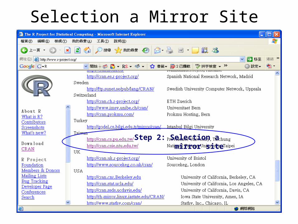
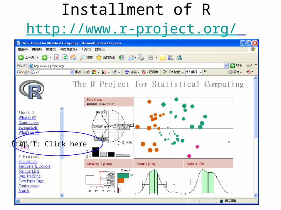
Selection a Mirror Site
Step 2: Selection a mirror site

Step 3: Selection OS for R
e.g., Windows

Clicking “base”
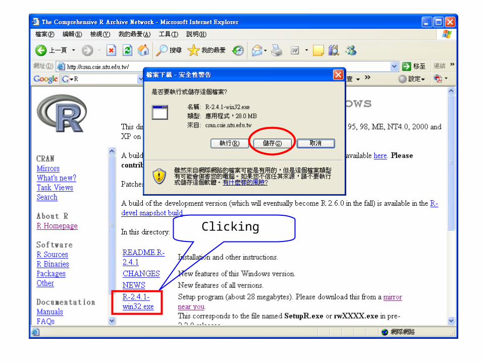
Clicking

Installation R
Double clicking R-icon for
installation R

Using R
1
2 3
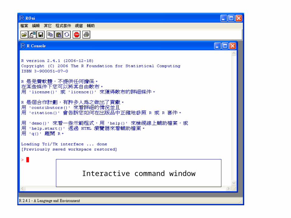
Interactive command window

Environment Commands > search() # loaded packages[1] ".GlobalEnv" "package:stats" "package:graphics" [4] "package:grDevices" "package:utils" "package:datasets" [7] "package:methods" "Autoloads" "package:base"
> ls() # Used objects [1] "bb" "col" "colorlut" "EdgeList" [5] "Edges" "EXP" "f“
> rm(bb) # remove object “bb”
> ?lm # ? Function name = look function
> args(lm) # look arguments in “lm”
> help(lm) #See detail of function (lm)
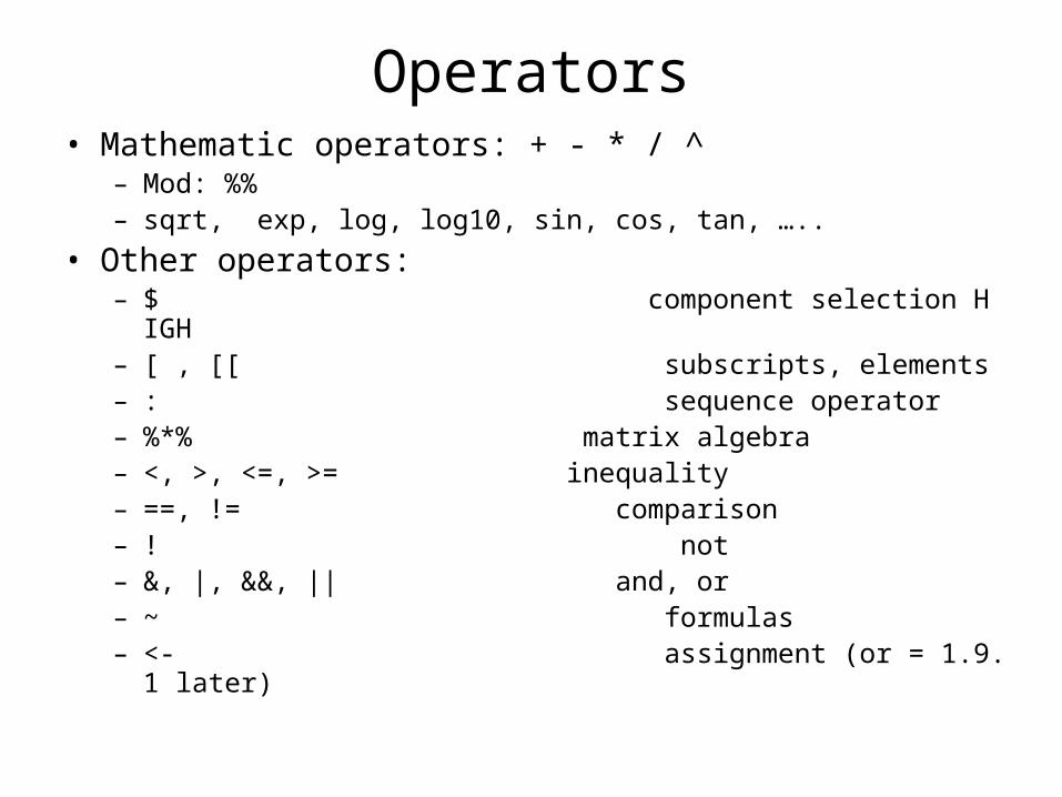
Operators• Mathematic operators: + - * / ^
– Mod: %%– sqrt, exp, log, log10, sin, cos, tan, …..
• Other operators:– $ component selection HIGH– [ , [[ subscripts, elements– : sequence operator– %*% matrix algebra – <, >, <=, >= inequality – ==, != comparison– ! not– &, |, &&, || and, or– ~ formulas– <- assignment (or = 1.9.1 later)
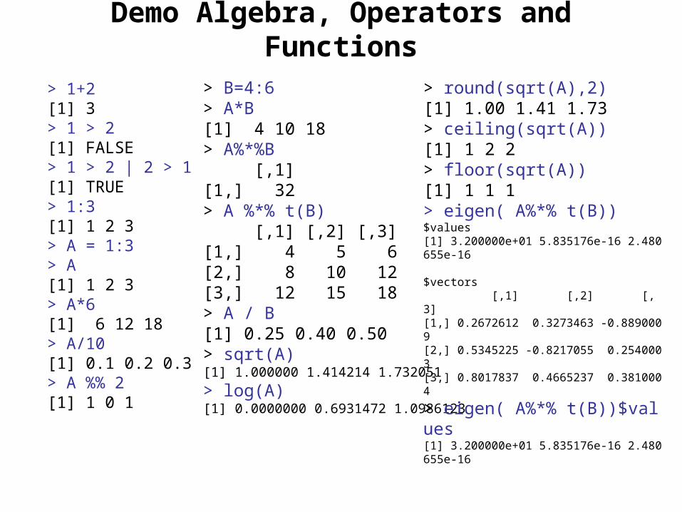
Demo Algebra, Operators and Functions
> 1+2[1] 3> 1 > 2[1] FALSE> 1 > 2 | 2 > 1[1] TRUE> 1:3[1] 1 2 3> A = 1:3> A[1] 1 2 3> A*6[1] 6 12 18> A/10[1] 0.1 0.2 0.3> A %% 2[1] 1 0 1
> B=4:6> A*B[1] 4 10 18> A%*%B [,1][1,] 32> A %*% t(B) [,1] [,2] [,3][1,] 4 5 6[2,] 8 10 12[3,] 12 15 18> A / B[1] 0.25 0.40 0.50> sqrt(A)[1] 1.000000 1.414214 1.732051
> log(A)[1] 0.0000000 0.6931472 1.0986123
> round(sqrt(A),2)[1] 1.00 1.41 1.73> ceiling(sqrt(A))[1] 1 2 2> floor(sqrt(A))[1] 1 1 1> eigen( A%*% t(B))$values[1] 3.200000e+01 5.835176e-16 2.480655e-16
$vectors [,1] [,2] [,3][1,] 0.2672612 0.3273463 -0.8890009[2,] 0.5345225 -0.8217055 0.2540003[3,] 0.8017837 0.4665237 0.3810004
> eigen( A%*% t(B))$values[1] 3.200000e+01 5.835176e-16 2.480655e-16
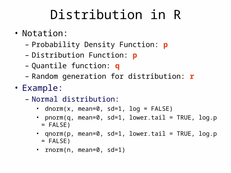
Distribution in R• Notation:
– Probability Density Function: p– Distribution Function: p– Quantile function: q– Random generation for distribution: r
• Example:– Normal distribution:
• dnorm(x, mean=0, sd=1, log = FALSE)• pnorm(q, mean=0, sd=1, lower.tail = TRUE, log.p = FALSE)• qnorm(p, mean=0, sd=1, lower.tail = TRUE, log.p = FALSE)• rnorm(n, mean=0, sd=1)
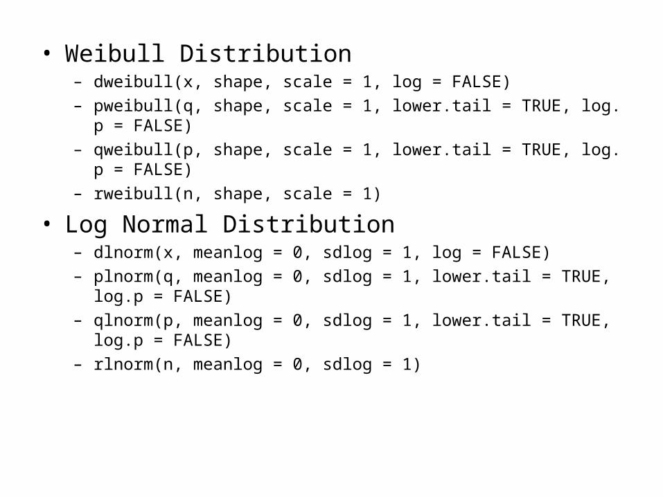
• Weibull Distribution– dweibull(x, shape, scale = 1, log = FALSE)
– pweibull(q, shape, scale = 1, lower.tail = TRUE, log.p = FALSE)
– qweibull(p, shape, scale = 1, lower.tail = TRUE, log.p = FALSE)
– rweibull(n, shape, scale = 1)
• Log Normal Distribution – dlnorm(x, meanlog = 0, sdlog = 1, log = FALSE)
– plnorm(q, meanlog = 0, sdlog = 1, lower.tail = TRUE, log.p = FALSE)
– qlnorm(p, meanlog = 0, sdlog = 1, lower.tail = TRUE, log.p = FALSE)
– rlnorm(n, meanlog = 0, sdlog = 1)

Statistical Functions
Excel RNORMSDIST pnorm(7.2,mean=5,sd=2)NORMSINV qnorm(0.9,mean=5,sd=2)LOGNORMDIST plnorm(7.2,meanlog=5,sdlog=2)LOGINV qlnorm(0.9,meanlog=5,sdlog=2)GAMMADIST pgamma(31, shape=3, scale =5)GAMMAINV qgamma(0.95, shape=3, scale =5)GAMMALN lgamma(4)WEIBULL pweibull(6, shape=3, scale =5)BINOMDIST pbinom(2,size=20,p=0.3)POISSON ppois(2, lambda =3)
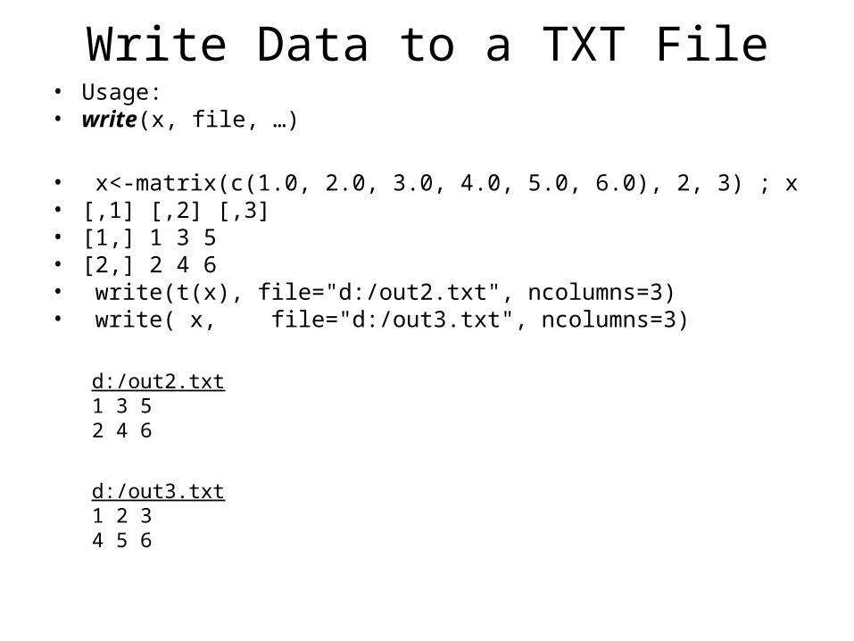
Write Data to a TXT File• Usage: • write(x, file, …)
• x<-matrix(c(1.0, 2.0, 3.0, 4.0, 5.0, 6.0), 2, 3) ; x• [,1] [,2] [,3]• [1,] 1 3 5• [2,] 2 4 6• write(t(x), file="d:/out2.txt", ncolumns=3)• write( x, file="d:/out3.txt", ncolumns=3)
d:/out2.txt1 3 52 4 6
d:/out3.txt1 2 34 5 6

Write Data to a CSV File• Usage: • write.table(x, file = "foo.csv", sep=", ",…) • Example:• x<-matrix(c(1.0, 2.0, 3.0, 4.0, 5.0, 6.0), 2, 3) ; x• [,1] [,2] [,3]• [1,] 1 3 5• [2,] 2 4 6• write.table(t(x), file="d:/out4.txt", sep=",", col.names=FALSE, row.n
ames=FALSE)• write.table(x, file="d:/out5.txt",sep=",", col.names=FALSE, row.nam
es=FALSE)d:/out4.txt1,23,45,6
d:/out5.txt1,3,52,4,6

Read TXT and CSV File• Usage: • read.table (file,…)
• X=read.table(file="d:/out2.txt"); X• V1 V2 V3• 1 1 3 5• 2 2 4 6• X=read.table(file="d:/out5.txt",sep=", ", header=FALSE); X
d:/out2.txt1 3 52 4 6
d:/out5.csv1,3,52,4,6
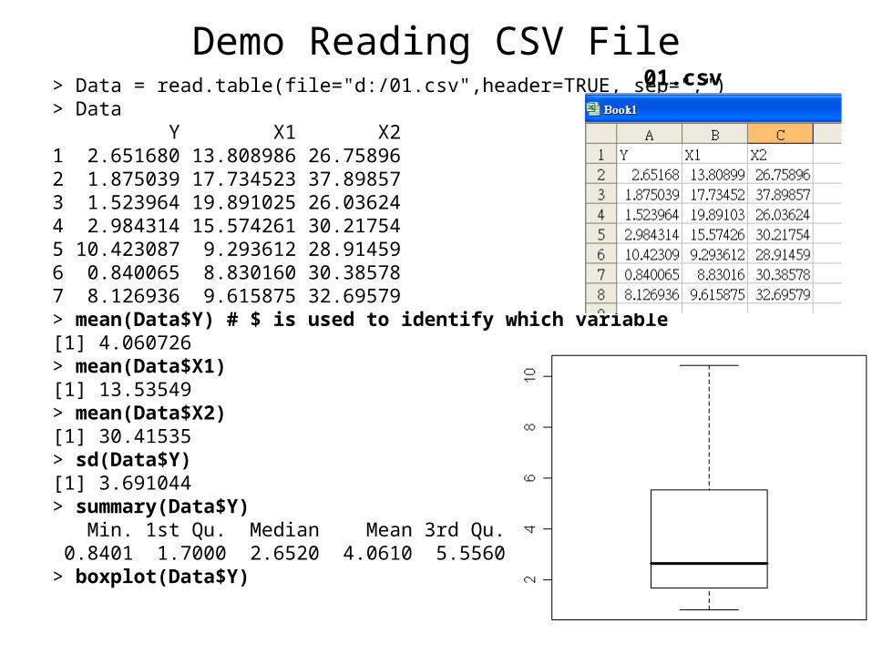
Demo Reading CSV File> Data = read.table(file="d:/01.csv",header=TRUE, sep=",")> Data Y X1 X21 2.651680 13.808986 26.758962 1.875039 17.734523 37.898573 1.523964 19.891025 26.036244 2.984314 15.574261 30.217545 10.423087 9.293612 28.914596 0.840065 8.830160 30.385787 8.126936 9.615875 32.69579> mean(Data$Y) # $ is used to identify which variable[1] 4.060726> mean(Data$X1)[1] 13.53549> mean(Data$X2)[1] 30.41535> sd(Data$Y)[1] 3.691044> summary(Data$Y) Min. 1st Qu. Median Mean 3rd Qu. Max. 0.8401 1.7000 2.6520 4.0610 5.5560 10.4200 > boxplot(Data$Y)
01.csv
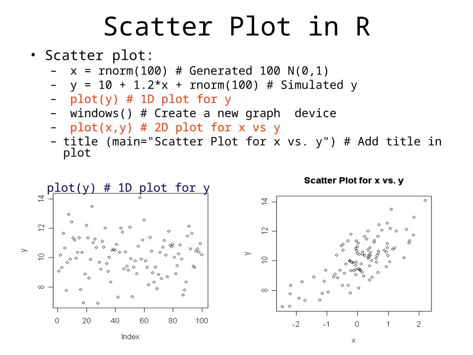
Scatter Plot in R • Scatter plot:
– x = rnorm(100) # Generated 100 N(0,1)– y = 10 + 1.2*x + rnorm(100) # Simulated y– plot(y) # 1D plot for y– windows() # Create a new graph device– plot(x,y) # 2D plot for x vs y– title (main="Scatter Plot for x vs. y") # Add title in plot
plot(y) # 1D plot for y

Scatterplot Matrices in R• A matrix of scatterplots is produced.
– Usage:• pairs(x, ...)
– Example: • X = matrix(rnorm(300),100,3)• pairs(X)

Box Plot in R• Box plot:
– Produce box-and-whisker plot of the given (grouped) values. – Usage: boxplot(x, ...)– Example1: Example2:
• X=rnorm(100) x=rnorm(100); y=rnorm(100);• boxplot(x) boxplot(x,y)
Q3 +1.5*IQR
Q1 -1.5*IQR
Q3
Q1Q2 = median ( x )IQR
Outliers
Outliers

Plot normal density
Kernel Density Plot
• Kernel Density: – density(x,…)– Kernel Density Plot:
• plot(density(x,…))
– Examples:• X= rlnorm(100,0,1)• plot(density(X))• Y= rweibull(100,1.5,1)• plot(density(Y))• x= rnorm(100, mean=3, sd=3)• plot(density(x))
Plot log-normal density
Plot weibull density

Probability Plots• Need installation R package : e1071
1
2
3
4
5
6
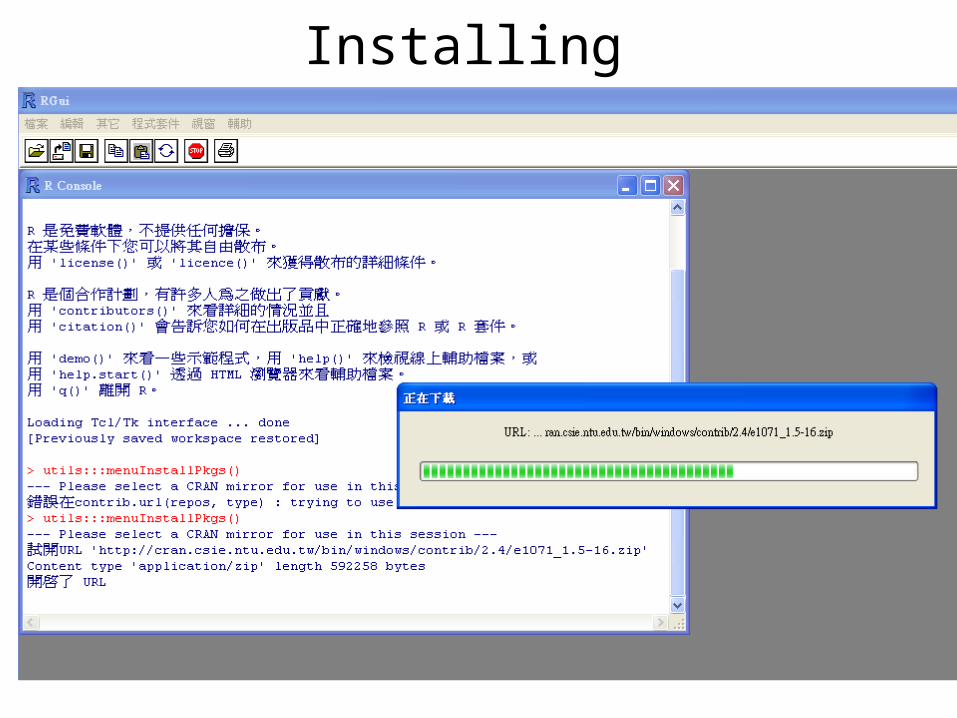
Installing
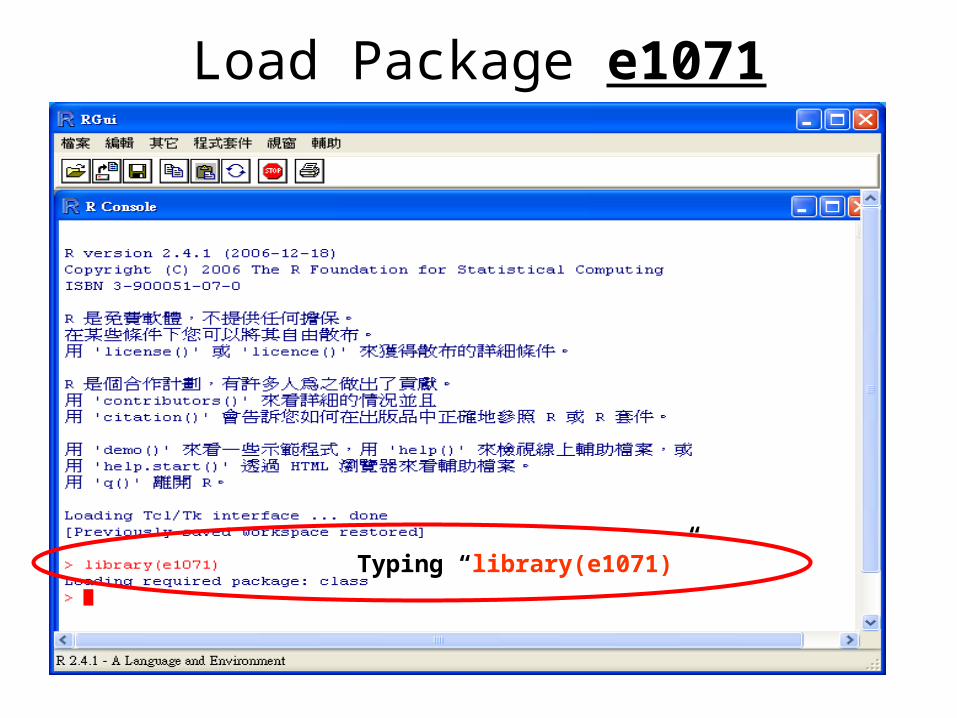
Load Package e1071
Typing “library(e1071)”
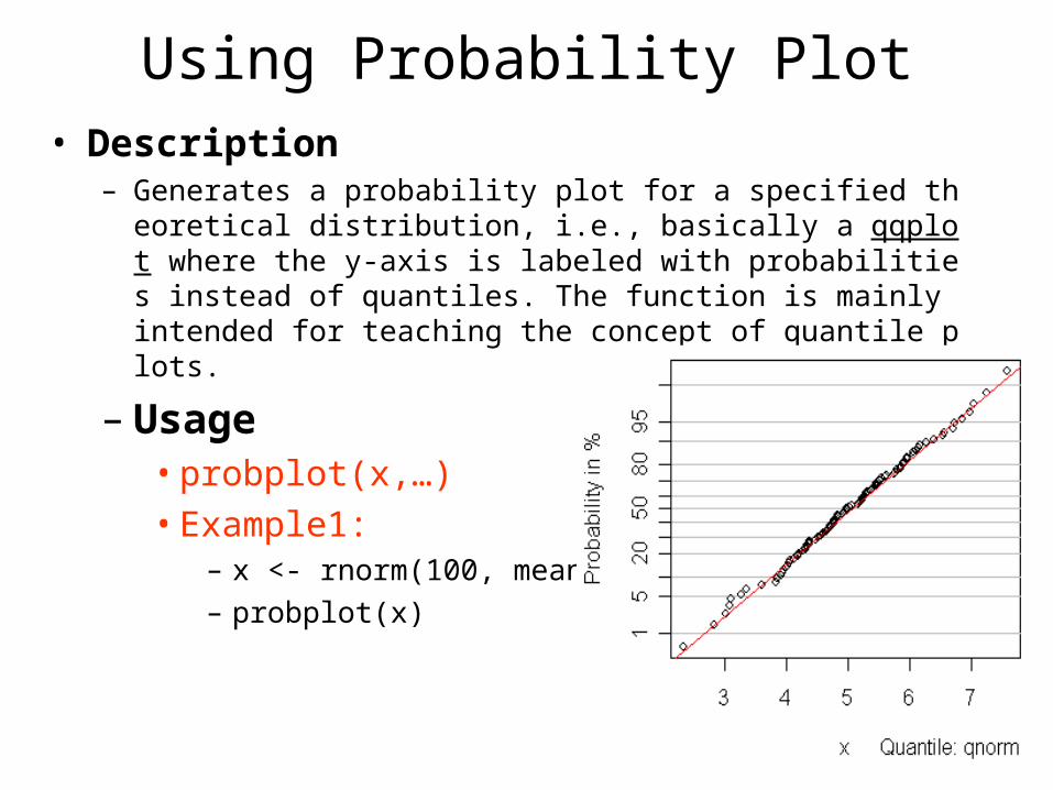
Using Probability Plot• Description
– Generates a probability plot for a specified theoretical distribution, i.e., basically a qqplot where the y-axis is labeled with probabilities instead of quantiles. The function is mainly intended for teaching the concept of quantile plots.
– Usage• probplot(x,…) • Example1:
– x <- rnorm(100, mean=5) – probplot(x)

More Examples• Example2:
– x <- rlnorm(100,meanlog = 3, sdlog = 2)– probplot(x, "qlnorm", meanlog = 3, sdlog = 2)
• Example 3:– x=rweibull(100, shape=2.5, scale = 3.5)– probplot(x,"qweibull", shape=2.5, scale = 3.5)
Pareto Chart
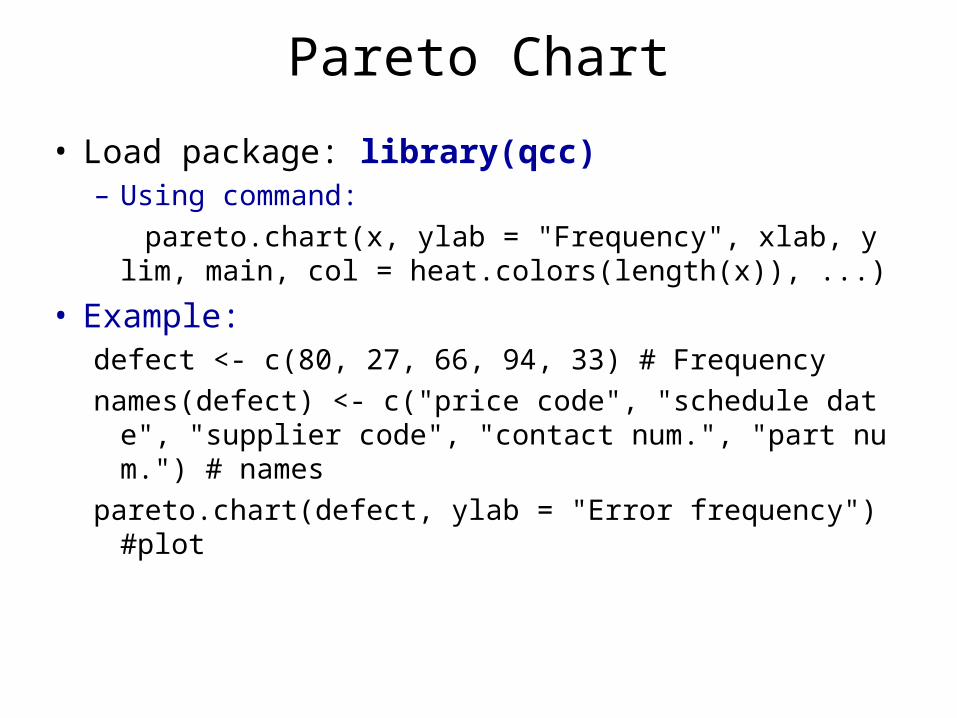
• Load package: library(qcc)– Using command:
pareto.chart(x, ylab = "Frequency", xlab, ylim, main, col = heat.colors(length(x)), ...)
• Example:defect <- c(80, 27, 66, 94, 33) # Frequency
names(defect) <- c("price code", "schedule date", "supplier code", "contact num.", "part num.") # names
pareto.chart(defect, ylab = "Error frequency")#plot
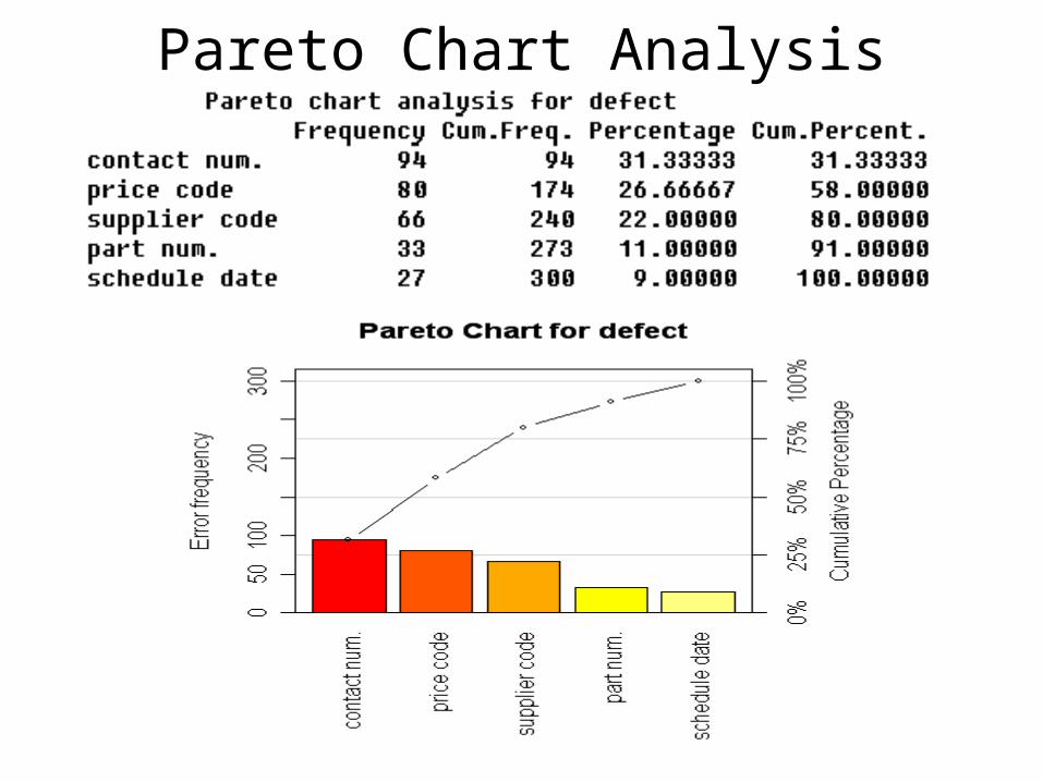
Pareto Chart Analysis
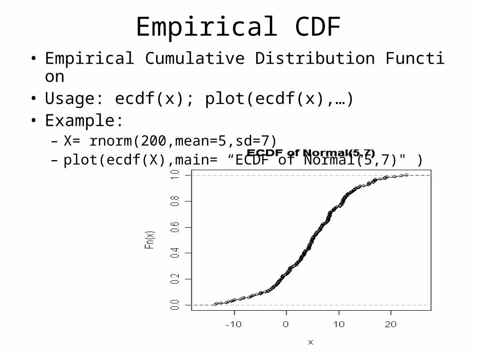
Empirical CDF• Empirical Cumulative Distribution Function • Usage: ecdf(x); plot(ecdf(x),…)• Example:
– X= rnorm(200,mean=5,sd=7)– plot(ecdf(X),main= “ECDF of Normal(5,7)" )

Histogram (1)• The generic function hist computes a histogram of the given data va
lues.
• Usage: hist(x, probability = !freq, ...) • Example:
– X=rlnorm(300,lmean=5, logsd=3)– hist(X) # Using default setting
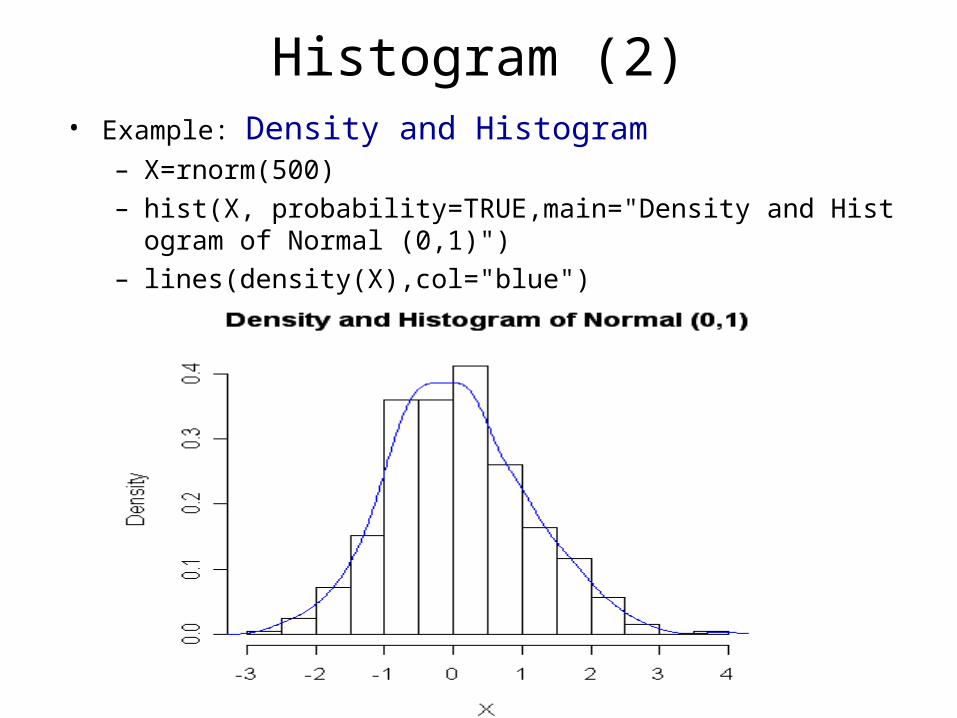
Histogram (2)• Example: Density and Histogram
– X=rnorm(500)– hist(X, probability=TRUE,main="Density and Histogram of Norm
al (0,1)")– lines(density(X),col="blue")