An introduction to control theory for PDEs Thomas I. Seidmanseidman/Papers/ctrl_thurnau.pdfAn introduction to control theory for PDEs Thomas I. Seidman Department of Mathematics and

An introduction to control theory for PDEs

Thomas I. Seidman

Department of Mathematics and StatisticsUMBC Baltimore, MD 21250

e-mail: 〈[email protected]〉

Abstract: A brief introduction to distributed parameter system theory gov-erned by linear partial differential equations:abstract ODEs and semigroups, duality of observation and nullcontrol, HUM,nullcontrolability and stabilization, geometry and the wave equation, local con-trol of the heat equation.

Much is like standard system theory (with Linear Algebra replaced by FunctionalAnalysis), but we also emphasize the role of geometry.

2007 Summer School: Optimization and Control with Applications in Modern Technologies 1/28

An outline:

1. Some examples and questions

2. Reformulation as abstract ODEs; Semigroups

3. A basic Duality Theorem

4. Some results


Example 1: an optimal control problem

Suppose we are given a region Ω ⊂ R2 and consider the heat equation (diffusion

equation)

(1)ut = uxx + uyy + ϕ on Q = (0, T )× Ω

u = 0 on (0, T )× ∂Ωu = u0 on Ω at t = 0

Fix a subregion ω ⊆ Ω.

Problem 1: Given u0 and a target u in L2(Ω), choose ϕ ∈ L2(Q) so as tominimize

(2) J (ϕ) =

∫ T

0

‖ϕ(t, ·)‖2 dt + λ‖u(T, ·)− u‖2

subject to the condition that ϕ(t, x, y) = 0 when (x, y) 6∈ ω.


What would we like to know?

1. Is (1) well-posed?

2. Is the minimum attained?[How does this depend on u0? on u? on T ? on ω?]

3. Which targets u can be reached exactly? are they dense? How might thisdepend on T ? on ω?

4. How can we compute the optimal control?Can we characterize the optimal control (first order optimality conditions)

5. What happens as λ→∞? [nullcontrol: u = 0]What are the asymptotics as T → 0?


Example 2: an observation problem

We again consider

(3)ut = uxx + uyy on Q = (0, T )× Ω

u = 0 on (0, T )× ∂Ωu = ? on Ω at t = 0

Problem 2: Given ω ⊂ Ω, we observe u on Qω = (0, T ) × ω and seek anestimate u for u(T, ·) — the state on all of Ω.



1. If y = u∣∣∣ω≡ 0 on Qω, does that imply u ≡ 0 on all of Q?

2. What would be the effect of observation noise?

3. What would be an ‘optimal’ map: y 7→ u[Is this linear? continuous?]

4. How is this problem related to the previous one?


Example 3: another optimal control problem

Suppose we are given a region Ω ⊂ R2 and consider the wave equation

(4)wtt = wxx + wyy + ϕ on Q = (0, T )× Ω

w = 0 on (0, T )× ∂Ωw = w0 wt = w1 on Ω at t = 0

Fix a subregion ω ⊆ Ω.

Problem 3: Given u0 = [w0, w1] and a target state u = [w0, w1] in H1(Ω)×L2(Ω), choose ϕ ∈ L2(Q) so as to minimize

(5) J (ϕ) =

∫ T

0

‖ϕ(t, ·)‖2 dt + λ‖u(T, ·)− u‖2

subject to the condition that ϕ(t, x, y) = 0 when (x, y) 6∈ ω.



1. All the same questions as for Example 1

. . .

2. How are these problems (Examples 1, 3) similar? different?


Semigroups and abstract ODEs:

Let S(t) : X → X : u0 7→ u(t) for the solution of the (linear, autonomous)

abstract ODE

(6) u′ = Au u(0) = u0

Assuming wellposedness, we have

(7)S(t + s) = S(t)S(s) S(0) = I

dS(t)

dt= AS(t) = S(t)A

S(t)u0 → u0 (all u0 ∈ X ) ‖S(t)‖ ≤Meωt (some M,ω)

The semigroup S(t) = etA is defined on X if:

A closed, D(A) dense, (λ− ω)n ‖(λ−A)−n‖ bounded.

[If t 7→ S(t) is analytic on a sector, then: ‖[−A]αS(t)‖ ≤Mt−αeωt.]


Dirichlet Laplacian:

We consider the Dirichlet Laplacian to be the (unbounded) linear operator on

X0 = L2(Ω) given by

(8)∆ : X0 = L2(Ω) ⊃ D(A)→ X0 : u 7→ uxx + uyy

with D(∆) =u ∈ H2(Ω) : u

∣∣∣∂Ω

= 0

This satisfies the conditions to generate a semigroup S(·) so, for Example 1,

(9)(1) ⇐⇒ u′ = ∆u + Bϕ, u(0) = u0

⇐⇒ u(t) = S(t)u0 +∫ t

0 S(t− s)Bϕ(s) ds

where B : U = L2(ω) → X .

For this Example the semigroup S(·) is analytic.


Two other examples:

The wave equation (4) wtt = ∆w + ϕ can be written as a first order system

u′ = Au + ϕ by setting

u =

(uv

)=

([−∆]1/2w

wt

)A =

(0 [−∆]1/2

[−∆]1/2 0

)ϕ =

(0ϕ

)Here S(·) is not analytic.

[Alternatively, u = (∇w, wt)T gives ut = ∇v, vt = ∇ · u.]


The system for a linear thermoelastic plate

(10) wtt + ∆2w − α∆ϑ = 0 ϑt −∆ϑ + α∆wt = ϕ

(control in the thermal component) can be put in first order form by setting

u =

ϑuv

=

ϑ∆wwt

A =

∆ 0 −α∆0 0 ∆α∆ −∆ 0

ϕ =

ϕ00


Some inverse problems:

Problem 4: We observe y(·) = Cu(·) on [0, T ] with u satisfying u′ = Au +

f, u(0) = 0 — f an unknown input which we would like to determine. We can thentreat this as an optimal control problem for the equation v′ = Av + ϕ, v(0) = 0:choosing the control ϕ to minimize J (ϕ) = ε‖ϕ‖2

U +λ‖Cv−y‖2U and then taking

ϕopt as the estimate for f .

Problem 5: Longitudinal vibration of a straight viscoelastic rod satisfies thelinearized equation wtt = wxx+εwxxt. Assume this is fixed at one end (w(t, 0) = 0)

and an unknown contact force f (t) at the other end ([wx+εwxt]∣∣∣x=`

= f ) produces

an observed motion y(·) = w(·, `). We wish to find f (·) by replacing it by a controlwhich minimizes the observation error ‖w(·, `)− y‖.

Problem 6: Let ut = uxx − qu with u(·, 0) = 0 and ux(·, `) = a(t). Choosea(·) for an experiment designed to determine the unknown function q = q(x) fromobservation of y(·) = u(·, `).


Abstract control problem:

The abstract version of the optimal control problem is then

Approximate u by STu0 + Bϕ with ‖ϕ‖U small.

with ST = S(T ) and, in view of (9),

B : U→ X : ϕ 7→∫ T

0

S(T − s)Bϕ(s) ds

where U is a Banach space of U -valued functions on [0, T ].

For the Hilbert space case U = L2([0, T ]→ U) of (2), minimizingJ (ϕ) = ‖ϕ‖2

U + λ‖STu0 + Bϕ − u‖2 gives the first order optimality condition:ϕ + B∗λ(STu0 + Bϕ− u) = 0

so ϕ = −λ(I + λB∗B)−1B∗(STu0 − u)


The adjoint problem:

We must compute the adjoint B∗: consider

(11) −v′ = A∗v, v(T ) = η so v(t) = S∗(T − t)η(referred to as the adjoint equation). Then

〈Bϕ, η〉 = 〈u(T ), v(T )〉 = 〈u(t), v(t)〉∣∣∣∣T0

=

∫ T

0

〈u, v〉′ dt

=

∫ T

0

[〈Au + Bϕ, v〉 + 〈u,−A∗v〉] dt

=

∫ T

0

〈ϕ,B∗v〉 dt

so B∗ : X∗ → U∗ : η 7→ y(·) = B∗v(·)

[Note that the map: y(·) 7→ v(0) = S∗(T )η — if it is defined — gives precisely theestimation of Example 2 (although there is a time reversal involved),]


The Duality Theorem:

What happens if λ → ∞ (exact nullcontrol: u = 0)? We assume that both

ST : X → X and B : U→ X are continuous.

Theorem 1. The following are equivalent:

1. For each u0 ∈ X there is a nullcontrol ϕ ∈ U so STu0 + Bϕ = 0 in X.

2. One has the range containment R(ST ) ⊂ R(B) in X

3. There is a continuous map: Γ : X → U such that ST + BΓ = 0

4. For solutions of the adjoint equation: −v′ = A∗v, one has an observationinequality:

(12) ‖v(0)‖X ≤ c‖B∗v(·)‖U∗so Γ1 : R(B∗)→ X∗ : B∗v(·) 7→ −v(0) is defined and continuous.

[If ‖ϕ‖U ≤ C‖u0‖ in 1., then this C is the same as in (12) and ‖Γ1‖ ≤ C.]


Proof of the Duality Theorem:

Clearly 1.⇐⇒2. and 3.⇒1. To show 1.⇒3., let U be the quotient space U/N (B)

and define an operator

M : X × U→ X : (u0, [ϕ]) 7→ STu0 + Bϕ

This is continuous so N (M) is closed — and is the graph of a linear operatorΓ0 : X → U : u0 7→ [ϕ] since [ϕ] is unique in N (M). As 1. means that Γ0 iseverywhere defined on the Banach space X , its continuity follows by the ClosedGraph Theorem; we can then appeal to the Michael Selection Theorem to get Γ.

Note that we may identify U∗ with R(B∗) and, by the earlier computationof B∗, the operators Γ0, Γ1 are indeed adjoints; hence 3.⇐⇒4.

[In a Hilbert space setting (U∗ = U), we can identify the quotient space U with thesubspaceN (B)⊥ = R(B∗) → U and Γ : X → U is linear; then ‖Γ‖ = C = ‖Γ1‖.This theorem is the heart of Lions’ Hilbert Uniqueness Method (HUM).]


A boundary control problem:

Unlike ODEs, one can have control which apparently does not appear in the

differential equation itself. For example, consider

(13)ut = uxx + uyy on Q = (0, T )× Ω

u = ϕ on (0, T )× ∂Ωu = u0 on Ω at t = 0

Problem 7: Much as for Problem 1 — except that the control appears in thechoice of boundary data, constrained so ϕ = 0 except on a specified set ω ⊂ ∂Ω,with the control space U a space of functions on Σω = [0, T ]× ω.[Similar problems of boundary control (or observation: Example 2) can be posedfor other equations, such as the wave equation.]

[Bϕ is defined as the value at T of the solution of the equation with control ϕ andinitial data u0 = 0. If this map is continuous: U→ X , then the Duality Theoremcontinues to apply. One must be very careful (especially for the wave equation)with appropriately specifying the spaces involved and checking regularity.]


A trick:

For a boundary control patch ω open in ∂Ω, there is a simple trick to reduce the

boundary problem above to Example 1, involving an interior control patch:

Artificially, add a ‘bump’ to Ω such that the interface between the bump and Ωlies within ω ⊂ ∂Ω; call the new region Ω′. Artificially define a control patch ω′ inthe interior of the bump, hence in Ω′. Embed X in a space of functions on Ω′ —e.g., extending each u0 as 0 on the bump. If one can then control to 0 on Ω′ by acontrol on ω′, then the trace on [0, T ]× ω of the resulting solution can be used asa nullcontrol for the original boundary control problem.[Essentially the same trick works for the observation problem of Example 2.]


A damping inequality and stabilization:

Our first damping inequality is: there are K,ϑ with ϑ < 1 for which:

for every u0 in X there is some ϕ on [0, T ] such that

(14) ‖STu0 + BT ϕ‖ ≤ ϑ‖u0‖ ‖ϕ‖U ≤ K‖u0‖Given (14), recursively set uj = u(jT ) = STuj−1 + BT ϕj−1 and then get ϕj on[jT, (j + 1)T ] from it (u0 ←7 uj). Concatenating these intervals gives ϕ on [0,∞)such that (for any (α < | lnϑ|/T )

Jα(ϕ) =

∫ ∞0

[‖ϕ‖2U + ‖u‖2]e2αt dt <∞

The map Γ : u0 7→ the Jα-minimizing control is linear and continuous. AssumingK : u 7→ [Γu](0) is continuous (evaluation at the initial point), autonomy givesϕ(·) in feedback form: ϕ(t) = Ku(t) so A+BK generates an exponentially stablesemigroup.

[We only mention the considerable work on use of the algebraic Riccati equation(ARE for operators on infinite dimensional Hilbert spaces) to obtain K.]


Two abstract results:

We know two abstract results to obtain nullcontrolability from damping:

Theorem 2. Suppose, much like (14), one has T,K, ϑ with ϑ < 1 such that:for each initial state u there exists u and a control ϕ on [0, T ] for which‖ϕ‖U ≤ K‖u‖ and ‖ST (u− u1) + BT ϕ‖ ≤ ϑ‖u‖. Then for each u0 there is anullcontrol ϕ such that ‖ϕ‖UT ≤ C‖u0‖ with C ≤ K/(1− ϑ).

Proof: Recursively obtain ϕj on [0, T ] and uj+1 = uj such that

‖ϕj‖ ≤ K‖uj‖ ‖uj+1‖ ≤ ϑ‖uj‖ ST (uj − uj+1) + BT ϕj = 0

Take ϕ =∑∞

0 ϕj and summing the telescopic series∑

ST (uj−uj+1)+BT ϕj = 0shows ϕ is a nullcontrol for u0.


Theorem 3. Suppose there exist c, d > 0 such that, for any τ > 0, one has:for each u0 there exists ϕ on [0, τ ] for which

‖ϕ‖U ≤ ec/τ‖u0‖, ‖Sτu0 + Bτ ϕ‖ ≤ e−d/τ‖u0‖.Then one has ‘rapid nullcontrolability’ (all T > 0): for each T, u0 there is anullcontrol ϕ on [0, T ] with ‖ϕ‖UT ≤ C‖u0‖ for C = ec/T if c > (c + d)c/d.

Proof: Choose c/(c + d) < r < 1 (so ε = 1 − (c/d)(1 − ϑ)/ϑ > 0 and setτ0 = (1 − ϑ)T so, with t0 = 0, tj+1 = tj + τj, one has the partition

⋃j[tj, tj+1)

for [0, T ). Recursively obtain ϕj on [tj, tj+1] and set uj+1 = Sτjuj + Bτj ϕj.Concatenating gives ϕ on [0, T ]. It is easy to see that ‖uj‖ → 0 so ϕ will be anullcontrol. A slightly messy estimation shows ‖ϕ‖U ≤ Σ‖ϕj‖ ≤ ec/T‖u0‖ withc = c/(1− r) and optimizing the choice of r concludes the proof.


Geometry and the wave equation:

For the classical wave equation disturbances/information propagate at speed 1,

so there is necessarily a minimum observation time to ‘see’ any part of the stateoutside the observation patch ω: the key to understanding the geometry of thewave equation is ray tracing with this propagation speed.

Consider the 1-D wave equationwtt = wxx corresponding to small transverse

vibrations of a string — which we fix at one end (w∣∣∣x=0≡ 0) with the deviation

of the other end (x = `) as control. Now think of this as a semi-infinite stringwithout control and with data vanishing outside [0, `] Ray tracing — here settingw(t, x) = f (x + t) + g(x − t) with f, g matching the data — shows that w,wtvanish within [0, `] for t > 2` so we can take w(·, `) for this solution as nullcontrol.Note that the longest ‘ray’ within Ω = (0, `), allowing for the reflection at x = 0,has length 2`: exactly the control time found.


Geometry and the wave equation, continued:

Let L be the sup of lengths of rays (geodesics), allowing for specular reflec-

tion at the noncontroling part of the boundary, until entering the control region.It was shown by Bardos-Lebeau-Rauch (1992) that the minimum time for null-controlability is, indeed, L. The necessity of this for nullcontrolability or observa-tion/prediction seems obvious (and trapped rays should preclude nullcontrolabilityfor any T at all), but one needs sufficiency.

Neglecting many technical difficulties, one notes from Scattering Theorythat (e.g., for “star-complemented regions”) in suitable time T at least a fixedfraction of the initial energy will exit through the control portion of the boundaryso, using this trace as ϕ, one obtains a damping inequality as in Theorem 2 andnullcontrolability follows.


Geometry and the heat equation:

Boundary nullcontrolability had been known for the 1-D case via classical har-

monic analysis and spectral expansion — separately for observation and for null-control as Theorem 1 was then unknown.

Essentially the result for the wave equation noted above was due to Russell(1973) and he also used this to show, by a harmonic analysis argument (compareMiller’s (2004) related use of the “transmutation method”) corresponding bound-ary nullcontrolability for the heat equation; Seidman (1976) showed how to obtainboundary nullcontrolability (using all of ∂Ω) directly from the 1-dimensional resultby embedding Ω in a cylinder. It was shown in (1984) that Russell’s argumentgave C = eO(1/T ) for the heat equation.

Nullcontrolability from an arbitrary open control patch ω ⊂ Ω was firstshown (Lebeau-Robbiano, 1995) using Carleman inequalities, a technique used toobtain a quantitative form of uniqueness from data on a patch. [This has messyenough technicalities not to describe it here.]


Rapid patch nullcontrolability of the heat equation:

We use instead an argument based on a deep theorem of Jerison-Lebeau about

eigenfunctions of ∆ (itself obtained using Carleman inequalities):

Theorem 4. (JL) Let (zj, λj) be the eigenpairs of ∆ so 0 < λ0 ≤ λj →∞.Then for open ω ⊂ Ω there is γ > 0 such that, for all σ > 0 and every functionw ∈ Zσ = spanzj : λj ≤ σ, one has

(15)

∫Ω

|w(s)|2 ds ≤ C2e2γ√σ

∫ω

|w(s)|2 ds

To show patch nullcontrolability of the heat equation, note that this is obviouswith control on all of Ω (C = O(1/

√T ) ). Split u0 = vσ+wσ withwσ ∈ Zσ, and use

the observation inequality for this whence Theorem 4 gives a similar inequality fromQω for Zσ with a factor eγ

√στ/2 whence nullcontrol with that estimate. The large

control spillover to vσ, is dominated, for large σ = (s/τ )2, by the e−στ/2 decay onthe uncontroled second half of [0, τ ]. Combining gives a damping inequality suitableto apply Theorem 3which shows that the heat equation is rapidly nullcontrolableon ω with control norm blowup C = eO(1/T ) as T → 0.


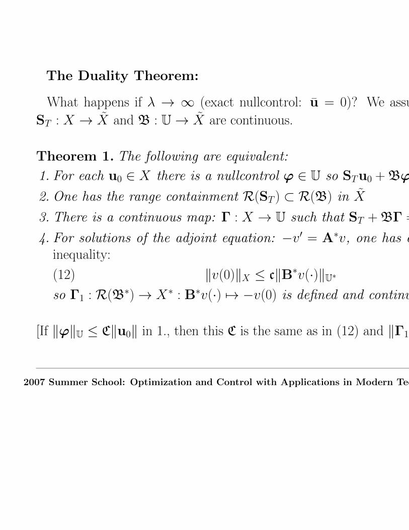
A couple of open problems:

We would be incomplete without noting at least a couple of open problems:

• The same argument as was used just above for the heat equation also showsrapid nullcontrolability for the thermoelastic plate with control on an interiorpatch ω in just one component. However, the trick noted earlier to get patchboundary nullcontrolability from this does not work for coupled systems if onewants control only in one component; a similar difficulty arises if the boundaryconditions are different for w, ϑ. How can one then show rapid nullcontrolabilityhere with C = eO(1/T )?

• For all of this we have implicitly assumed ω to be an open subset of Ω (or of∂Ω). For open ω, what are the asymptotics as ω shrinks to a point? Can oneobtain similar results if control is restricted instead to a subset of Q (or of Σ)having positive measure? [This kind of question arises, e.g., in connection withbang-bang theorems for constrained control.]


• And of course we have not touched yet on problems involving constrained controlor nonlinear equations or non-additive control or shape control or . . .


Documents

An introduction to control theory for PDEs Thomas I. Seidmanseidman/Papers/ctrl_thurnau.pdfAn introduction to control theory for PDEs Thomas I. Seidman Department of Mathematics and