An Introduction to Copulae - Daniel Berg · Daniel Berg Introduction to Copulae. Introduction Deﬁnitions and theorems Examples Dependence concepts Copula Families Archimedean copulae

IntroductionDefinitions and theorems

ExamplesDependence concepts

Copula FamiliesArchimedean copulae

Estimating copula parametersSimulating from copulae

Higher Dimensional CopulaeApplication

Copula goodness-of-fit testsSummary

An Introduction to Copulae

Daniel Berg

University of Oslo & Norwegian Computing Center

Statistics seminar.

NTNU – March-14-2006.

Daniel Berg Introduction to Copulae







Outline

1. Introduction

2. Definitions and Theorems

3. Dependence Concepts

4. Copula Families

5. Estimation

6. Simulation

7. Higher Dimensional Copulae

8. Application

9. Goodness-of-fit

10. Concluding remarks and further reading








Historical background

1. Introduction

⊲ Dependency modelling

⊲ Linear correlation coefficient - a measure of linear dependence

⊲ In e.g. financial markets we often see non-linear dependency structures

⊲ Elliptical distributions - linear dependence structure - correlation coefficientmeaningful

⊲ Non-elliptical distributions - alternative measures of dependence needed ⇒Copulae

⊲ Any multivariate distribution function can serve as a copula








Historical background

1.1. Brief historical background:

⊲ 1940’s: Hoeffding studies properties of multivariate distributions

⊲ 1959: The word copula appears for the first time (Sklar)

⊲ 1999: Introduced to financial applications (Embrechts, McNeil, Straumann)

⊲ 2006: Several insurance companies, banks and other financial institutions applycopulae as a risk management tool








Attractive features


Definition (Copula)A d-dimensional copula is a multivariate distribution, C, with standard uniform marginaldistributions.

Theorem (Sklar)Every multivariate distribution F , with margins, F1, F2, . . . , Fd can be written as

F (x1, . . . , xd ) = C(F1(x1), . . . , Fd (xd )), (2.1)

for some copula C.








Attractive features


⊲ Given a random vector X = (X1, . . . , Xd ) the copula of their joint distributionfunction may be extracted from equation (2.1):

C(u1, . . . , ud ) = F (F−11 (u1), . . . , F−1

d (ud )),

where the F−1i ’s are the quantile functions of the margins.

⊲ The copula is often represented by its density function c(u):

C(u) = P(U1 ≤ u1, U2 ≤ u2, . . . , Ud ≤ ud ) =

Z u1

0. . .

Z ud

0c(u)du,








Attractive features


⊲ For the implicit copula of an absolutely continuous joint df F with strictlycontinuous marginal df’s F1, . . . , Fd , the copula density is given by

c(u) =f (F−1

1 (u1), . . . , F−1d (ud ))

f1(F−11 (u1)) · · · fd (F−1

d (u1)).

⊲ Hence,

c(F1(x1), . . . , Fd (xd )) =h(x1, . . . , xd )

f1(x1) · · · fd (xd ).

⊲ This means that a general d-dimensional density can be written as

f (x1, . . . , xd ) = c(F1(x1), . . . , Fd (xd )) · f1(x1) · · · fd (xd )

for some copula density c(·).








Attractive features

2.1. Attractive features of copulae:

⊲ A copula describes how the marginals are tied together in the joint distribution

⊲ The joint df is decomposed into the marginal dfs and a copula

⊲ The marginal dfs and the copula can be modelled and estimated separately,independent of each other

⊲ Given a copula, we can obtain many multivariate distributions by selectingdifferent marginal dfs

⊲ The copula is invariant under increasing and continuous transformations








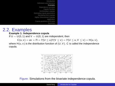
2.2. ExamplesExample 1: Independence copulaIf U ∼ U(0, 1) and V ∼ U(0, 1) are independent, then

C(u, v) = uv = Π = P(U ≤ u)P(V ≤ v) = P(U ≤ u, V ≤ v) = H(u, v),

where H(u, v) is the distribution function of (U, V ). C is called the independencecopula.

0.0 0.2 0.4 0.6 0.8 1.0

0.0

0.2

0.4

0.6

0.8

1.0

u

v

Figure: Simulations from the bivariate independence copula.








2.2 Examples

Example 2: Gaussian copula (implicit)

CGaρ (u, v) =

Z Φ−1(u)

−∞

Z Φ−1(v)

−∞

1

2π(1 − ρ2)1/2exp

(− x2 − 2ρxy + y2

2(1 − ρ2)

)dxdy ,

where ρ is the linear correlation coefficient.Example 3: Student’s t copula (implicit)

Ctρ,ν(u, v) =

Z t−1(u)

−∞

Z t−1(v)

−∞

1

2π(1 − ρ2)1/2

(1 +

x2 − 2ρxy + y2

ν(1 − ρ2)

)−(ν+2)/2

dxdy ,

where ν is the degrees of freedom and ρ is the linear correlation coefficient.








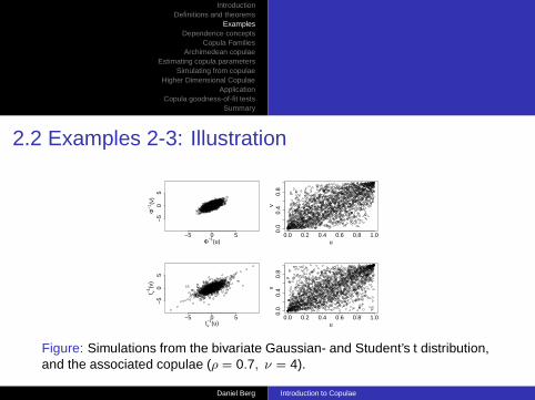
2.2 Examples 2-3: Illustration

−5 0 5

−5

05

Φ−1(u)

Φ−1

(v)

0.0 0.2 0.4 0.6 0.8 1.0

0.0

0.4

0.8

u

v

−5 0 5

−5

05

tν−1(u)

t ν−1(v

)

0.0 0.2 0.4 0.6 0.8 1.0

0.0

0.4

0.8

u

v

Figure: Simulations from the bivariate Gaussian- and Student’s t distribution,and the associated copulae (ρ = 0.7, ν = 4).








2.2 ExamplesExample 4: Clayton copula (explicit)

CClδ (u, v) = (u−δ + v−δ − 1)−1/δ,

where 0 < δ < ∞ is the parameter controlling the dependence. Perfect dependence isobtained if δ → ∞, while δ → 0 implies independence.

0.0 0.2 0.4 0.6 0.8 1.0

0.0

0.2

0.4

0.6

0.8

1.0

u

v

Figure: Simulations from the bivariate Clayton copula (δ = 3).








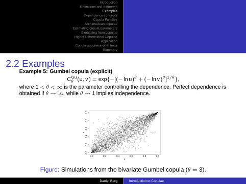
2.2 ExamplesExample 5: Gumbel copula (explicit)

CGuθ (u, v) = exp{−[(− ln u)θ + (− ln v)θ]1/θ},

where 1 < θ < ∞ is the parameter controlling the dependence. Perfect dependence isobtained if θ → ∞, while θ → 1 implies independence.

0.0 0.2 0.4 0.6 0.8 1.0

0.0

0.2

0.4

0.6

0.8

1.0

u

v

Figure: Simulations from the bivariate Gumbel copula (θ = 3).








3. Dependence Concepts

We will consider the following dependence measures:

⊲ Linear correlation

⊲ Concordance

◦ Kendall’s tau◦ Spearman’s rho

⊲ Tail dependence








3.1. Linear correlation

ρ(X , Y ) =Cov(X , Y )pVar(X)Var(Y )

.

⊲ Sensitive to outliers

⊲ Measures the "average dependence" between X and Y

⊲ Invariant under strictly increasing linear transformations

⊲ May be misleading in situations where multivariate df is not elliptical








3.1. Linear correlation

−3 −1 0 1 2 3

−3

−2

−1

01

23

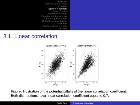
Gaussian copula (ρ=0.7)

Φ−1(u)

Φ−1

(v)

−3 −1 0 1 2 3

−3

−2

−1

01

23

Clayton copula (δ=2.015)

Φ−1(u)

Φ−1

(v)

Figure: Illustration of the potential pitfalls of the linear correlation coefficient.Both distributions have linear correlation coefficient equal to 0.7.








3.2. Concordance

Let (xi , yi ) and (xj , yj) be two observations from a random vector (X , Y ) of continuousrandom variables.

⊲ Concordance: (xi − xj )(yi − yj ) > 0

⊲ Discordance: (xi − xj )(yi − yj) < 0

Let (X1, Y1) and (X2, Y2) be independent vectors of cont. random variables with jointdf’s H1 and H2 and copulae C1 and C2, respectively. Let Q define the differencebetween the prob. of concordance and discordance of (X1, Y1) and (X2, Y2):

Q = P ((X1 − X2)(Y1 − Y2) > 0) − P ((X1 − X2)(Y1 − Y2) < 0)

= Q(C1, C2) = 4Z 1

0

Z 1

0C2(u, v)dC1(u, v) − 1.








3.2.1. Kendall’s tau

ρτ (X , Y ) = Q(C, C) = 4Z 1

0

Z 1

0C(u, v)dC(u, v) − 1

= 4E(C(U, V )) − 1.

⊲ Less sensitive to outliers


⊲ Invariant under strictly increasing transformations

⊲ Depends only on the copula of (X , Y )

⊲ For elliptical copulae: cor(X , Y ) = sin`

π2 ρτ

´








3.2.2. Spearmans’s rho

ρS(X , Y ) = 3Q(C,Π)

= 12Z 1

0

Z 1

0uvdC(u, v) − 3

= 12Z 1

0

Z 1

0C(u, v)dudv − 3.

⊲ Less sensitive to outliers


⊲ Invariant under strictly increasing transformations

⊲ Depends only on the copula of (X , Y )

⊲ ρS(X , Y ) = ρ(FX (X), FY (Y ))

⊲ For elliptical copulae: cor(X , Y ) = 2sin`

π6 ρS

´








3.3. Tail dependenceLet (X , Y ) be a r.v. with marginal df’s FX and FY . The coefficient of upper and lowertail dependence of (X , Y ) is defined as:

λu(X , Y ) = limα→1

P(Y > F−1Y (α)|X > F−1

X (α)),

λl (X , Y ) = limα→0

P(Y ≤ F−1Y (α)|X ≤ F−1

X (α)).

I.e. the tail dependence is the prob. of observing a large(small) Y , given that X islarge(small). If λu > 0 (λl > 0), then we say that (X , Y ) has upper (lower) taildependence.

⊲ Gaussian copula: λu = λl = 2 limx→∞ Φ“

xp

1 − ρ/p

1 + ρ”

= 0

⊲ Student-t copula: λu = λl = 2tν+1

“−√

ν + 1p

(1 − ρ)/(1 + ρ)”

. Asymptotic

tail dependence, even when ρ = 0.

⊲ Clayton copula: λu = 0, λl = 2−1/δ.

⊲ Gumbel copula: λl = 0, λu = 2 − 21/θ .








4. Copula Families

We will consider the two most important families of copulae:

⊲ Elliptical copulae

⊲ Archimedean copulae








4.1. Elliptical Copulae

⊲ Implied by well-known multivariate df’s, derived through Sklar’s theorem

⊲ Extends the multivariate normal Nd (µ,Σ).

⊲ Extend to arbitrary dimensions and are rich in parameters. A d-dim ellipticalcopula has at least d(d − 1)/2 parameters

⊲ Easy to simulate

⊲ Drawback: Do not have closed form expressions and are restricted to have radialsymmetry

Examples: Gaussian copula, Student’s t copula








4.2. Archimedean Copulae

An Archimedean copula is defined as follows:

C(u, v) = ϕ−1(ϕ(u) + ϕ(v)).

The function ϕ is called the generator of the copula.

⊲ Allow for a great variety of dependence structures

⊲ Closed form expressions

⊲ Not derived from mv df’s using Sklar’s theorem

⊲ Drawback: Higher dimensional extensions difficult

Examples: Clayton copula, Gumbel copula








4.2. Archimedean Copulae

Example 1: Clayton copulaThe generator function for the Clayton copula is given by ϕ(t) = (t−δ − 1)/δ, whereδ ∈ (0,∞). This gives the Clayton copula:

Cδ(u, v) = ϕ−1(ϕ(u) + ϕ(v)) = (u−δ + v−δ − 1)−1/δ.

The Clayton copula has lower tail dependence.Example 2: Gumbel copulaThe generator function for the Gumbel copula is given by ϕ(t) = (− ln t)θ , whereθ ≥ 1. This gives the Gumbel copula:

Cθ(u, v) = ϕ−1(ϕ(u) + ϕ(v)) = exp(−[(− ln u)θ + (− ln v)θ ]1/θ).

The Gumbel copula has upper tail dependence.








5. Estimating Copula ParametersFully parametric method:

⊲ Denoted Inference functions for margins (IFM) method.

⊲ Assumes parametric univariate marginal distributions.

⊲ Parameters of margins are first estimated, then each parametric margin isplugged into the copula likelihood, and this full likelihood is maximized.

⊲ Success depends upon finding appropriate parametric models for the margins,which is not always straightforward

Semi-parametric method:

⊲ Denoted the pseudo-likelihood or canonical maximum likelihood (CML) method

⊲ No parametric assumptions for the margins, use empirical cdf’s, then plug intolikelihood








5.1 Estimation - Elliptical copulae

Gaussian copula:

⊲ Correlation matrix R (d(d − 1)/2 parameters)

⊲ ML estimator: bR = arg maxR∈PPn

j=1 log c(U j ; R), where the pseudo samplesU j are generated using either the IFM or the CML method.

Student’s t copula:

⊲ Correlation matrix R and degree-of-freedom ν (1 + d(d − 1)/2 parameters)

⊲ ML wrt R and ν simultaneously difficult

⊲ Simpler: two-stage approach in which R is estimated first using Kendall’s tau,and then the pseudo-likelihood function is maximized wrt ν.








5.2 Estimation - Archimedean copulae

Clayton and Gumbel copulae:

⊲ One parameter, δ and θ respectively

⊲ Numerical optimization of likelihood

⊲ Bivariate - utilize the following relationships to Kendall’s tau:

bδ =2bρτ

1 − bρτ, bθ =

1

1 − bρτ.








6. Simulating from Copulae

Gaussian copula:

⊲ Simulate X ∼ Nd (0, R)

⊲ Set U = (Φ(X1), . . . , Φ(Xd )) or U = (F (X1), . . . , F (Xd )) where the F ’s are thequantile functions

Student’s t copula:

⊲ Simulate X ∼ td (0, R, ν)

⊲ Set U = (tν(X1), . . . , tν(Xd )) or U = (F (X1), . . . , F (Xd )) where the F ’s are thequantile functions








6. Simulating from CopulaeClayton copula:By noting that the inverse of the generator is equal to the Laplace transform of aGamma variate X ∼ Ga(1/δ, 1), the simulation algorithm becomes:

⊲ Simulate a gamma variate X ∼ Ga(1/δ, 1)

⊲ Simulate d iid U(0, 1) variables V1, . . . , Vd

⊲ Return U =“(1 − log V1

X )−1/δ, . . . , (1 − log VdX )−1/δ

”

Gumbel copula:By noting that the inverse of the generator function is equal to the Laplace transform ofa positive stable variate X ∼ St(1/θ, 1, γ, 0), where γ =

`cos

`π2θ

´´θ and θ > 1, thesimulation algorithm becomes:

⊲ Simulate a positive stable variate X ∼ St(1/θ, 1, γ, 0)

⊲ Simulate d iid U(0, 1) variables V1, . . . , Vd

⊲ Return U =

„exp

„−“− log V1

X

”1/θ«

, . . . , exp„−“− log Vd

X

”1/θ««








6. Simulating from CopulaeIn general we could apply the conditional marginal cdf’s:

Fi|1,...,i−1(ui |u1, . . . , ui−1) =∂ i−1C(u1, . . . , ui)

∂u1 · · · ∂ui−1

ffi∂ i−1C(u1, . . . , ui−1)

∂u1 · · · ∂ui−1.

The simulation algorithm then becomes:

⊲ Simulate a rv u1 from U(0, 1),

⊲ Simulate a rv u2 from F2|1(·|u1),

...

⊲ Simulate a rv ud from Fd|1,...,d−1(·|u1, . . . , ud−1).

⊲ Generally means simulating a rv Vi from U(0, 1) from whichui = F−1

i|1,...,i−1(Vi |u1, . . . , ui−1) can be obtained, if necessary by numerical root

finding.








7. Higher Dimensional Copulae

I. Copulae with at least d(d − 1)/2 bivariate dependence parameters:

⊲ Build multivariate copulae from bivariate copula

⊲ Based on iteratively mixing conditional copulae

⊲ Very flexible tool for dependency modelling

⊲ Does not require any assumption of conditional independence

⊲ Also referred to as ’Vines’ (Cooke and Bedford, 2002)

⊲ Drawback: difficult, slow, depends heavily on permutation








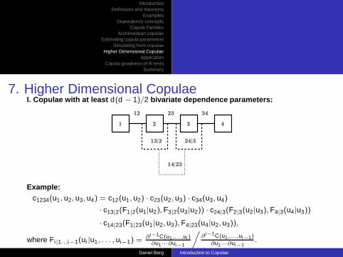
7. Higher Dimensional CopulaeI. Copulae with at least d(d − 1)/2 bivariate dependence parameters:

3

13|2 24|3

12 23 34

14|23

21 4

Example:c1234(u1, u2, u3, u4) = c12(u1, u2) · c23(u2, u3) · c34(u3, u4)

· c13|2(F1|2(u1|u2), F3|2(u3|u2)) · c24|3(F2|3(u2|u3), F4|3(u4|u3))

· c14|23(F1|23(u1|u2, u3), F4|23(u4|u2, u3)),

where Fi|1...i−1(ui |u1, . . . , ui−1) = ∂ i−1C(u1,...,ui )∂u1···∂ui−1

ffi∂ i−1C(u1,...,ui−1)

∂u1···∂ui−1.








7. Higher Dimensional CopulaeII. Archimedean copulae with d − 1 bivariate dependence parameters:

⊲ Build multivariate copulae from bivariate copula

⊲ Based on iteratively mixing conditional copulae

⊲ Less flexible but more intuitive and faster than ’vines’

⊲ Only applicable to Archimedean copulae with strict generator functions

C3(u1, u2, u3) = ϕ−1[ϕ(u1) + ϕ(u2) + ϕ(ud )]

= ϕ−1[ϕ(ϕ−1[ϕ(u1) + ϕ(u2)]) + ϕ(u3)]

= C2(C2(u1, u2), u3),

⇒ Cd (u1, . . . , ud ) = C2(Cd−1(u1, . . . , ud−1), ud ).

Example:

C3(u1, u2, u3) = ϕ−12 [ϕ2 ◦ ϕ−1

1 [ϕ1(u1) + ϕ1(u2)] + ϕ2(u3)].








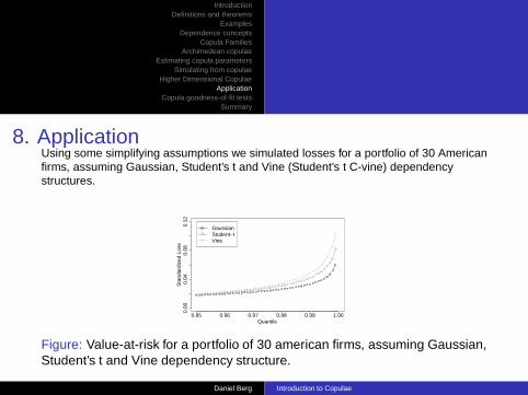
8. ApplicationUsing some simplifying assumptions we simulated losses for a portfolio of 30 Americanfirms, assuming Gaussian, Student’s t and Vine (Student’s t C-vine) dependencystructures.

0.95 0.96 0.97 0.98 0.99 1.00

0.00

0.04

0.08

0.12

Quantile

Sta

ndar

dize

d Lo

ss

GaussianStudent−tVine

Figure: Value-at-risk for a portfolio of 30 american firms, assuming Gaussian,Student’s t and Vine dependency structure.








9. Copula Goodness-of-fit Testing

⊲ Special case of testing for multivariate density models

⊲ Complicated due to the unspecified marginal df’s. Asymptotic distributionalproperties becomes very difficult to derive ⇒ p-values obtained throughsimulation.

⊲ χ2- and other tests based on binning the probability space will not be feasible inhigher dimensions as the need for data would be too great.

⊲ Some tests focus on multivariate smoothing procedures. These arecomputationally very demanding in high dimensions.

⊲ A more promising class of tests project the multivariate problem to a univariateproblem, then apply a univariate GOF statistic, e.g. Anderson-Darling (AD).

⊲ We may base the testing on the probability integral transform (PIT).








9.1 Probability Integral Transform (PIT)

⊲ The PIT transforms a set of dependent variables into a new set of independentU(0, 1) variables, given the multivariate distribution.

⊲ A universally applicable way of creating a set of iid U(0, 1) variables from anydata set with known distribution

⊲ First introduced by Rosenblatt (1952)

⊲ Inverse of simulation

⊲ GOF: the observed copula is PIT assuming a H0 copula. Then a test ofindependence is performed.








9.1 Probability Integral Transform (PIT)DEFINITION: Probability Integral TransformLet X = (X1, . . . , Xd ) denote a random vector with marginal distributionsFi(xi ) = P(Xi ≤ xi ) and conditional distributions F (Xi ≤ xi |X1 = x1, . . . , Xi−1 = xi−1)for i = 1, . . . , d . The PIT of X is defined as T (X ) = (T1(X1), . . . , Td (Xd )) where Ti(Xi )is defined as follows:

T1(X1) = P(X1 ≤ x1) = FX1(x1),

T2(X2) = P(X2 ≤ x2|X1 = x1) = FX2|X1(x2|x1),

...

Td (Xd ) = P(Xd ≤ xd |X1 = x1, . . . , Xd−1 = xd−1) = FXd |X1...Xd−1(xd |x1, . . . , xd−1).

The random variables Zi = Ti(Xi ), for i = 1, . . . , d are uniformly and independentlydistributed on [0, 1]d . F (xi |x1, . . . , xi−1) is found by

Fi|1...i−1(ui |u1, . . . , ui−1) =∂ i−1C(u1, . . . , ui)

∂u1 · · · ∂ui−1

ffi∂ i−1C(u1, . . . , ui−1)

∂u1 · · · ∂ui−1.








9.2 Proposed testsG: Breymann et al. (2003)

Y Gj =

dX

i=1

Φ−1(zji )2, j = 1, . . . , n,

G(w) = P“

Fχ2d(Y G ≤ w)

”, w ∈ [0, 1].

⊲ Coincides with the tests proposed by Malevergne and Sornette (2003) when thelatter is based on PIT. Also coincides with the test proposed by Chen et al. (2004).

⊲ Very fast

⊲ Tail weight

⊲ NOT consistent








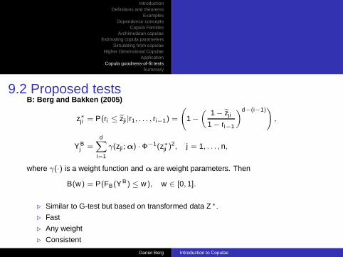
9.2 Proposed testsB: Berg and Bakken (2005)

z∗ji = P(ri ≤ ezji |r1, . . . , ri−1) =

1 −

„1 − ezji

1 − ri−1

«d−(i−1)!

,

Y Bj =

dX

i=1

γ(zji ; α) · Φ−1(z∗ji )

2, j = 1, . . . , n,

where γ(·) is a weight function and α are weight parameters. Then

B(w) = P(FB(Y B) ≤ w), w ∈ [0, 1].

⊲ Similar to G-test but based on transformed data Z∗.

⊲ Fast

⊲ Any weight

⊲ Consistent








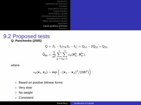
9.2 Proposed testsQ: Panchenko (2005)

Q = 〈f1 − f2|κd |f1 − f2〉 = Q11 − 2Q12 + Q22,

bQkp =1

n2

nX

jk =1

nX

jp=1

κd (X jkk , X

jpp ),

where

κd (x1, x2) = expn−‖x1 − x2‖2/(2dh2)

o.

⊲ Based on positive bilinear forms

⊲ Very slow

⊲ No weight

⊲ Consistent








9.2 Proposed tests

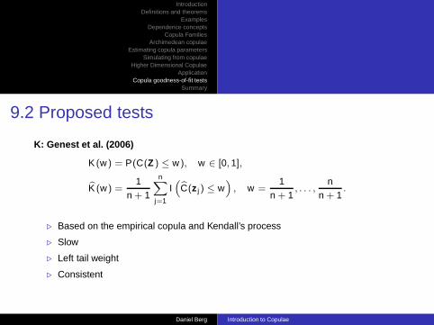
K: Genest et al. (2006)

K (w) = P(C(Z ) ≤ w), w ∈ [0, 1],

bK (w) =1

n + 1

nX

j=1

I“bC(z j) ≤ w

”, w =

1

n + 1, . . . ,

n

n + 1.

⊲ Based on the empirical copula and Kendall’s process

⊲ Slow

⊲ Left tail weight

⊲ Consistent








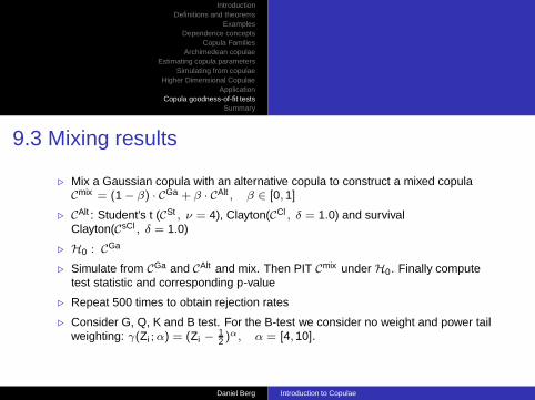
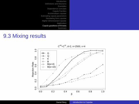
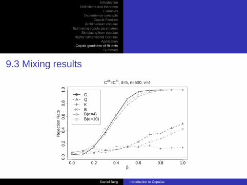
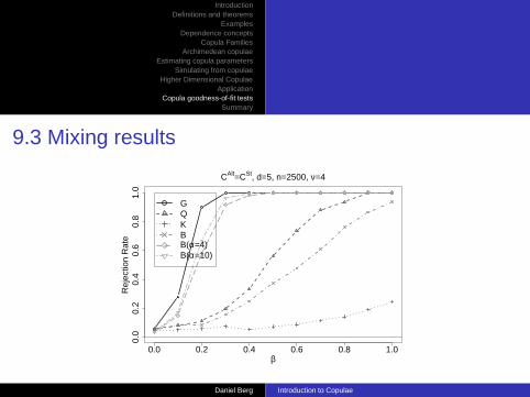
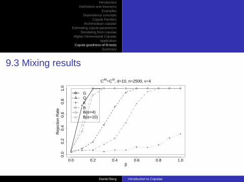
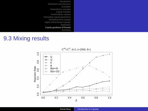
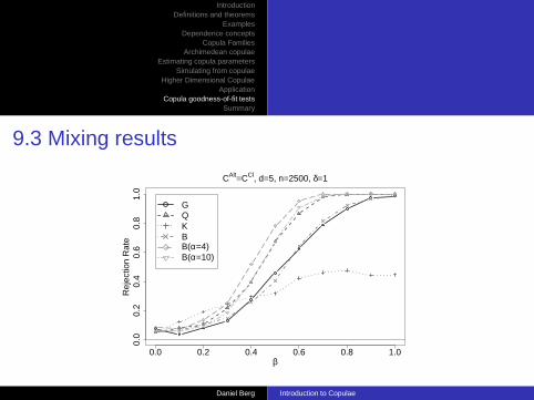
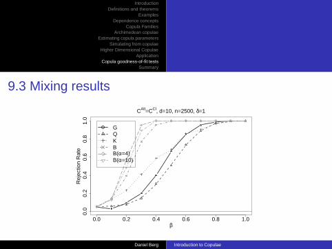
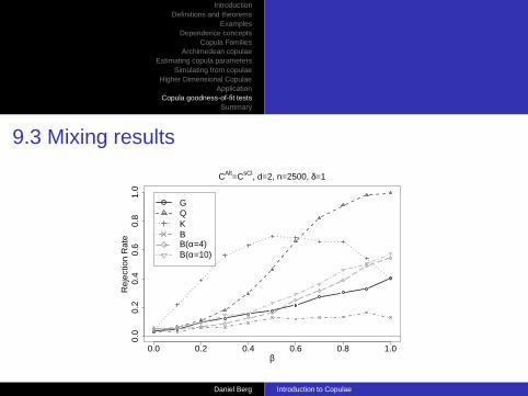
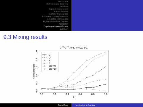
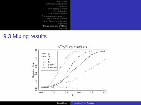
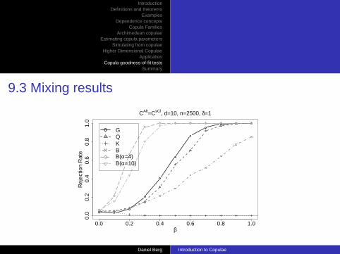
9.3 Mixing results

⊲ Mix a Gaussian copula with an alternative copula to construct a mixed copulaCmix = (1 − β) · CGa + β · CAlt , β ∈ [0, 1]

⊲ CAlt : Student’s t (CSt , ν = 4), Clayton(CCl , δ = 1.0) and survivalClayton(CsCl , δ = 1.0)

⊲ H0 : CGa

⊲ Simulate from CGa and CAlt and mix. Then PIT Cmix under H0. Finally computetest statistic and corresponding p-value

⊲ Repeat 500 times to obtain rejection rates

⊲ Consider G, Q, K and B test. For the B-test we consider no weight and power tailweighting: γ(Zi ; α) = (Zi − 1

2 )α, α = [4, 10].








9.3 Mixing results

0.0 0.2 0.4 0.6 0.8 1.0

0.0

0.2

0.4

0.6

0.8

1.0

β

Rej

ectio

n R

ate

CAlt=CSt, d=2, n=500, ν=4

GQKBB(α=4)B(α=10)








9.3 Mixing results

0.0 0.2 0.4 0.6 0.8 1.0

0.0

0.2

0.4

0.6

0.8

1.0

β

Rej

ectio

n R

ate

CAlt=CSt, d=2, n=2500, ν=4

GQKBB(α=4)B(α=10)








9.3 Mixing results

0.0 0.2 0.4 0.6 0.8 1.0

0.0

0.2

0.4

0.6

0.8

1.0

β

Rej

ectio

n R

ate

CAlt=CSt, d=5, n=500, ν=4

GQKBB(α=4)B(α=10)








9.3 Mixing results

0.0 0.2 0.4 0.6 0.8 1.0

0.0

0.2

0.4

0.6

0.8

1.0

β

Rej

ectio

n R

ate

CAlt=CSt, d=5, n=2500, ν=4

GQKBB(α=4)B(α=10)








9.3 Mixing results

0.0 0.2 0.4 0.6 0.8 1.0

0.0

0.2

0.4

0.6

0.8

1.0

β

Rej

ectio

n R

ate

CAlt=CSt, d=10, n=2500, ν=4

GQKBB(α=4)B(α=10)








9.3 Mixing results

0.0 0.2 0.4 0.6 0.8 1.0

0.0

0.2

0.4

0.6

0.8

1.0

β

Rej

ectio

n R

ate

CAlt=CCl, d=2, n=500, δ=1

GQKBB(α=4)B(α=10)








9.3 Mixing results

0.0 0.2 0.4 0.6 0.8 1.0

0.0

0.2

0.4

0.6

0.8

1.0

β

Rej

ectio

n R

ate

CAlt=CCl, d=2, n=2500, δ=1

GQKBB(α=4)B(α=10)








9.3 Mixing results

0.0 0.2 0.4 0.6 0.8 1.0

0.0

0.2

0.4

0.6

0.8

1.0

β

Rej

ectio

n R

ate

CAlt=CCl, d=5, n=500, δ=1

GQKBB(α=4)B(α=10)








9.3 Mixing results

0.0 0.2 0.4 0.6 0.8 1.0

0.0

0.2

0.4

0.6

0.8

1.0

β

Rej

ectio

n R

ate

CAlt=CCl, d=5, n=2500, δ=1

GQKBB(α=4)B(α=10)








9.3 Mixing results

0.0 0.2 0.4 0.6 0.8 1.0

0.0

0.2

0.4

0.6

0.8

1.0

β

Rej

ectio

n R

ate

CAlt=CCl, d=10, n=2500, δ=1

GQKBB(α=4)B(α=10)








9.3 Mixing results

0.0 0.2 0.4 0.6 0.8 1.0

0.0

0.2

0.4

0.6

0.8

1.0

β

Rej

ectio

n R

ate

CAlt=CsCl, d=2, n=500, δ=1

GQKBB(α=4)B(α=10)








9.3 Mixing results

0.0 0.2 0.4 0.6 0.8 1.0

0.0

0.2

0.4

0.6

0.8

1.0

β

Rej

ectio

n R

ate


GQKBB(α=4)B(α=10)








9.3 Mixing results

0.0 0.2 0.4 0.6 0.8 1.0

0.0

0.2

0.4

0.6

0.8

1.0

β

Rej

ectio

n R

ate


GQKBB(α=4)B(α=10)








9.3 Mixing results

0.0 0.2 0.4 0.6 0.8 1.0

0.0

0.2

0.4

0.6

0.8

1.0

β

Rej

ectio

n R

ate


GQKBB(α=4)B(α=10)








9.3 Mixing results

0.0 0.2 0.4 0.6 0.8 1.0

0.0

0.2

0.4

0.6

0.8

1.0

β

Rej

ectio

n R

ate

CAlt=CsCl, d=10, n=2500, δ=1

GQKBB(α=4)B(α=10)








10. Summary

⊲ Linear correlation coefficient not sufficient outside the world of ellipticaldistributions ⇒ alternative dependence measures

⊲ Copula families: Elliptical, Archimedean

⊲ Estimation and simulation

⊲ Complex multivariate highly dependent models can be built, based on bivariatecopulae

⊲ Significant impacts, i.e. on portfolio VaR

⊲ Goodness-of-fit:

◦ Bivariate: several candidates◦ Dimension > 2: B-test


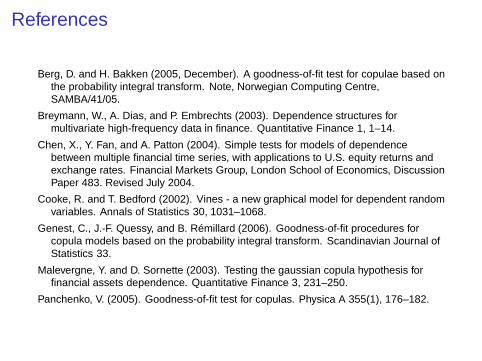
References

Berg, D. and H. Bakken (2005, December). A goodness-of-fit test for copulae based onthe probability integral transform. Note, Norwegian Computing Centre,SAMBA/41/05.

Breymann, W., A. Dias, and P. Embrechts (2003). Dependence structures formultivariate high-frequency data in finance. Quantitative Finance 1, 1–14.

Chen, X., Y. Fan, and A. Patton (2004). Simple tests for models of dependencebetween multiple financial time series, with applications to U.S. equity returns andexchange rates. Financial Markets Group, London School of Economics, DiscussionPaper 483. Revised July 2004.

Cooke, R. and T. Bedford (2002). Vines - a new graphical model for dependent randomvariables. Annals of Statistics 30, 1031–1068.

Genest, C., J.-F. Quessy, and B. Rémillard (2006). Goodness-of-fit procedures forcopula models based on the probability integral transform. Scandinavian Journal ofStatistics 33.

Malevergne, Y. and D. Sornette (2003). Testing the gaussian copula hypothesis forfinancial assets dependence. Quantitative Finance 3, 231–250.

Panchenko, V. (2005). Goodness-of-fit test for copulas. Physica A 355(1), 176–182.

Documents

An Introduction to Copulae - Daniel Berg · Daniel Berg Introduction to Copulae. Introduction Deﬁnitions and theorems Examples Dependence concepts Copula Families Archimedean copulae