Embed Size (px)
Citation preview
An Introduction to Cryptography
Mohamed Barakat, Christian Eder, Timo Hanke
September 20, 2018

Preface
Second Edition
Lecture notes of a class given during the summer term 2017 at the University of Kaiserslautern. Thenotes are based on lecture notes by Mohamed Barakat and Timo Hanke [BH12] (see also below).Other good sources and books are, for example, [Buc04, Sch95, MVO96].
Many thanks to Raul Epure for proofreading and suggestions to improve the lecture notes.
First Edition
These lecture notes are based on the course “Kryptographie” given by Timo Hanke at RWTH AachenUniversity in the summer semester of 2010. They were amended and extended by several topics,as well as translated into English, by Mohamed Barakat for his course “Cryptography” at TU Kaiser-slautern in the winter semester of 2010/11. Besides the literature given in the bibliography section,our sources include lectures notes of courses held by Michael Cuntz, Florian Heß, Gerhard Hiß andJürgen Müller. We would like to thank them all.
Mohamed Barakat would also like to thank the audience of the course for their helpful remarksand questions. Special thanks to Henning Kopp for his numerous improvements suggestions. Alsothanks to Jochen Kall who helped locating further errors and typos. Daniel Berger helped me withsubtle formatting issues. Many thanks Daniel.
i
Contents
Second Edition . . . . . . . . . . . . . . . . . . . . . . . . . . . . . . . . . . . . . . . . . . . . . . iFirst Edition . . . . . . . . . . . . . . . . . . . . . . . . . . . . . . . . . . . . . . . . . . . . . . . . i
Contents ii
1 Introduction 1
2 Basic Concepts 52.1 Quick & Dirty Introduction to Complexity Theory . . . . . . . . . . . . . . . . . . . . . 52.2 Underlying Structures . . . . . . . . . . . . . . . . . . . . . . . . . . . . . . . . . . . . . . 72.3 Investigating Security Models . . . . . . . . . . . . . . . . . . . . . . . . . . . . . . . . . 11
3 Modes of Ciphers 133.1 Block Ciphers . . . . . . . . . . . . . . . . . . . . . . . . . . . . . . . . . . . . . . . . . . . 133.2 Modes of Block Ciphers . . . . . . . . . . . . . . . . . . . . . . . . . . . . . . . . . . . . . 143.3 Stream Ciphers . . . . . . . . . . . . . . . . . . . . . . . . . . . . . . . . . . . . . . . . . . 233.4 A Short Review of Historical Ciphers . . . . . . . . . . . . . . . . . . . . . . . . . . . . . 25
4 Information Theory 274.1 A Short Introduction to Probability Theory . . . . . . . . . . . . . . . . . . . . . . . . . 274.2 Perfect Secrecy . . . . . . . . . . . . . . . . . . . . . . . . . . . . . . . . . . . . . . . . . . 314.3 Entropy . . . . . . . . . . . . . . . . . . . . . . . . . . . . . . . . . . . . . . . . . . . . . . . 35
5 Pseudorandom Sequences 475.1 Introduction . . . . . . . . . . . . . . . . . . . . . . . . . . . . . . . . . . . . . . . . . . . . 475.2 Linear recurrence equations and pseudorandom bit generators . . . . . . . . . . . . . 485.3 Finite fields . . . . . . . . . . . . . . . . . . . . . . . . . . . . . . . . . . . . . . . . . . . . . 535.4 Statistical tests . . . . . . . . . . . . . . . . . . . . . . . . . . . . . . . . . . . . . . . . . . 625.5 Cryptographically secure pseudorandom bit generators . . . . . . . . . . . . . . . . . 66
6 Modern Symmetric Block Ciphers 706.1 Feistel cipher . . . . . . . . . . . . . . . . . . . . . . . . . . . . . . . . . . . . . . . . . . . . 706.2 Data Encryption Standard (DES) . . . . . . . . . . . . . . . . . . . . . . . . . . . . . . . 716.3 Advanced Encryption Standard (AES) . . . . . . . . . . . . . . . . . . . . . . . . . . . . 74
7 Candidates of One-Way Functions 777.1 Complexity classes . . . . . . . . . . . . . . . . . . . . . . . . . . . . . . . . . . . . . . . . 777.2 Squaring modulo n . . . . . . . . . . . . . . . . . . . . . . . . . . . . . . . . . . . . . . . . 78
ii
CONTENTS iii
7.3 Quadratic residues . . . . . . . . . . . . . . . . . . . . . . . . . . . . . . . . . . . . . . . . 797.4 Square roots . . . . . . . . . . . . . . . . . . . . . . . . . . . . . . . . . . . . . . . . . . . . 817.5 One-way functions . . . . . . . . . . . . . . . . . . . . . . . . . . . . . . . . . . . . . . . . 837.6 Trapdoors . . . . . . . . . . . . . . . . . . . . . . . . . . . . . . . . . . . . . . . . . . . . . . 847.7 The Blum-Goldwasser construction . . . . . . . . . . . . . . . . . . . . . . . . . . . . . . 85
8 Public Key Cryptosystems 868.1 RSA . . . . . . . . . . . . . . . . . . . . . . . . . . . . . . . . . . . . . . . . . . . . . . . . . 868.2 ElGamal . . . . . . . . . . . . . . . . . . . . . . . . . . . . . . . . . . . . . . . . . . . . . . . 908.3 The Rabin cryptosystem . . . . . . . . . . . . . . . . . . . . . . . . . . . . . . . . . . . . . 918.4 Security models . . . . . . . . . . . . . . . . . . . . . . . . . . . . . . . . . . . . . . . . . . 93
9 Primality tests 959.1 Probabilistic primality tests . . . . . . . . . . . . . . . . . . . . . . . . . . . . . . . . . . . 959.2 Deterministic primality tests . . . . . . . . . . . . . . . . . . . . . . . . . . . . . . . . . . 100
10 Integer Factorization 10310.1 Pollard’s p− 1 method . . . . . . . . . . . . . . . . . . . . . . . . . . . . . . . . . . . . . . 10310.2 Pollard’s ρ method . . . . . . . . . . . . . . . . . . . . . . . . . . . . . . . . . . . . . . . . 10410.3 Fermat’s method . . . . . . . . . . . . . . . . . . . . . . . . . . . . . . . . . . . . . . . . . 10510.4 Dixon’s method . . . . . . . . . . . . . . . . . . . . . . . . . . . . . . . . . . . . . . . . . . 10510.5 The quadratic sieve . . . . . . . . . . . . . . . . . . . . . . . . . . . . . . . . . . . . . . . . 107
11 Elliptic curves 10911.1 The projective space . . . . . . . . . . . . . . . . . . . . . . . . . . . . . . . . . . . . . . . 10911.2 The group structure (E,+) . . . . . . . . . . . . . . . . . . . . . . . . . . . . . . . . . . . 11411.3 Elliptic curves over finite fields . . . . . . . . . . . . . . . . . . . . . . . . . . . . . . . . . 12011.4 Lenstra’s factorization method . . . . . . . . . . . . . . . . . . . . . . . . . . . . . . . . . 12411.5 Elliptic curves cryptography (ECC) . . . . . . . . . . . . . . . . . . . . . . . . . . . . . . 126
12 Attacks on the discrete logarithm problem 12812.1 Specific attacks . . . . . . . . . . . . . . . . . . . . . . . . . . . . . . . . . . . . . . . . . . 12812.2 General attacks . . . . . . . . . . . . . . . . . . . . . . . . . . . . . . . . . . . . . . . . . . 130
13 Digital signatures 13213.1 Basic Definitions & Notations . . . . . . . . . . . . . . . . . . . . . . . . . . . . . . . . . . 13213.2 Signatures using OWF with trapdoors . . . . . . . . . . . . . . . . . . . . . . . . . . . . 13313.3 Hash functions . . . . . . . . . . . . . . . . . . . . . . . . . . . . . . . . . . . . . . . . . . 13413.4 Signatures using OWF without trapdoors . . . . . . . . . . . . . . . . . . . . . . . . . . 135
A Some analysis 137A.1 Real functions . . . . . . . . . . . . . . . . . . . . . . . . . . . . . . . . . . . . . . . . . . . 137
Bibliography 138

Chapter 1
Introduction
Cryptology consists of two branches:
Cryptography is the area of constructing cryptographic systems.
Cryptanalysis is the area of breaking cryptographic systems.
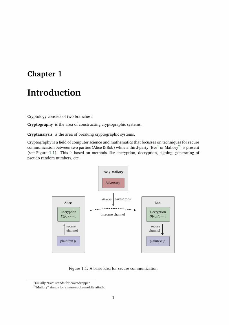
Cryptography is a field of computer science and mathematics that focusses on techniques for securecommunication between two parties (Alice & Bob) while a third-party (Eve1 or Mallory2) is present(see Figure 1.1). This is based on methods like encryption, decryption, signing, generating ofpseudo random numbers, etc.
Eve / Mallory
Adversary
Alice
EncryptionE(p, k) = c
plaintext p
Bob
DecryptionD(c, k′) = p
plaintext p
insecure channel
attacks eavesdrops
securechannel
securechannel
Figure 1.1: A basic idea for secure communication
1Usually “Eve” stands for eavesdropper.2“Mallory” stands for a man-in-the-middle attack.
1
2 CHAPTER 1. INTRODUCTION
The four ground principles of cryptography are
Confidentiality Defines a set of rules that limits access or adds restriction on certain information.
Data Integrity Takes care of the consistency and accuracy of data during its entire life-cycle.
Authentication Confirms the truth of an attribute of a datum that is claimed to be true by someentity.
Non-Repudiation Ensures the inability of an author of a statement resp. a piece of information todeny it.
Nowadays there are in general two different schemes: On the one hand, there are symmetricschemes, where both, Alice and Bob, need to have the same key in order to encrypt their com-munication. For this, they have to securely exchange the key initially. On the other hand, sinceDiffie and Hellman’s key exchange idea from 1976 (see also Example 1.1 (3) and Chapter 8) therealso exists the concept of asymmetric schemes where Alice and Bob both have a private and a publickey. The public key can be shared with anyone, so Bob can use it to encrypt a message for Alice.But only Alice, with the corresponding private key, can decrypt the encrypted message from Bob.
In this lecture we will discover several well-known cryptographic structures like RSA (Rivest-Shamir-Adleman cryptosystem), DES (Data Encryption Standard), AES (Advanced EncryptionStandard), ECC (Elliptic Curve Cryptography), and many more. All these structures have twomain aspects:
1. There is the security of the structure itself, based on mathematics. There is a standardiza-tion process for cryptosystems based on theoretical research in mathematics and complexitytheory. Here our focus will lay in this lecture.
2. Then we have the implementation of the structures in devices, e.g. SSL, TLS in your webbrowser or GPG for signed resp. encrypted emails. These implementations should not di-verge from the theoretical standards, but must still be very fast and convenient for the user.
It is often this mismatch between these requirements that leads to practical attacks of theoreticallysecure systems, e.g. [Wik16b, Wik16c, Wik16e].
Before we start defining the basic notation let us motivate the following with some historicallyknown cryptosystems:
Example 1.1.
1. One of the most famous cryptosystems goes back to Julius Ceasar: Caesar’s cipher does thefollowing: Take the latin alphabet and apply a mapping A 7→ 0, B 7→ 1, . . . , Z 7→ 25. Now weapply a shifting map
x 7→ (x + k) mod 26
for some secret k ∈ Z. For example, ATTACK maps to CVVCEM for k = 2. This describes theencryption process. The decryption is applied via the map
y 7→ (y − k) mod 26
with the same k. Clearly, both parties need to know k in advance. Problems with this cipher:Same letters are mapped to the same shifted letters, each language has its typical distribu-tion of letters, e.g. E is used much more frequently in the English language than K. Besidesinvestigating only single letters one can also check for letter combinations of length 2-3, etc.
3
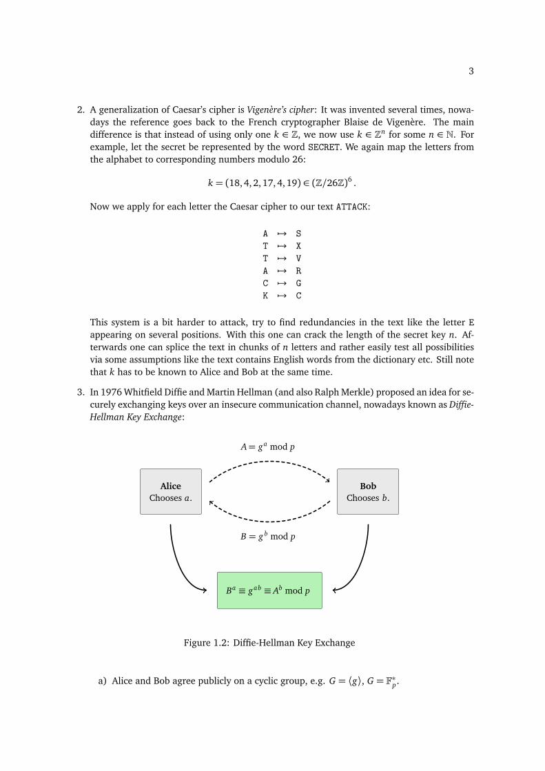
2. A generalization of Caesar’s cipher is Vigenère’s cipher: It was invented several times, nowa-days the reference goes back to the French cryptographer Blaise de Vigenère. The maindifference is that instead of using only one k ∈ Z, we now use k ∈ Zn for some n ∈ N. Forexample, let the secret be represented by the word SECRET. We again map the letters fromthe alphabet to corresponding numbers modulo 26:
k = (18, 4, 2, 17, 4, 19) ∈ (Z/26Z)6 .
Now we apply for each letter the Caesar cipher to our text ATTACK:
A 7→ ST 7→ XT 7→ VA 7→ RC 7→ GK 7→ C
This system is a bit harder to attack, try to find redundancies in the text like the letter Eappearing on several positions. With this one can crack the length of the secret key n. Af-terwards one can splice the text in chunks of n letters and rather easily test all possibilitiesvia some assumptions like the text contains English words from the dictionary etc. Still notethat k has to be known to Alice and Bob at the same time.
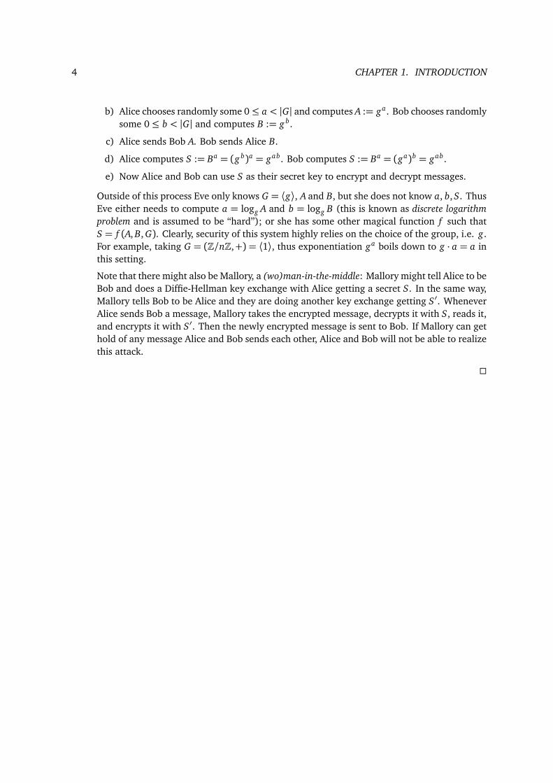
3. In 1976 Whitfield Diffie and Martin Hellman (and also Ralph Merkle) proposed an idea for se-curely exchanging keys over an insecure communication channel, nowadays known as Diffie-Hellman Key Exchange:
AliceChooses a.
BobChooses b.
A= ga mod p
B = g b mod p
Ba ≡ gab ≡ Ab mod p
Figure 1.2: Diffie-Hellman Key Exchange
a) Alice and Bob agree publicly on a cyclic group, e.g. G = ⟨g⟩, G = F∗p.
4 CHAPTER 1. INTRODUCTION
b) Alice chooses randomly some 0≤ a < |G| and computes A := ga. Bob chooses randomlysome 0≤ b < |G| and computes B := g b.
c) Alice sends Bob A. Bob sends Alice B.
d) Alice computes S := Ba = (g b)a = gab. Bob computes S := Ba = (ga)b = gab.
e) Now Alice and Bob can use S as their secret key to encrypt and decrypt messages.
Outside of this process Eve only knows G = ⟨g⟩, A and B, but she does not know a, b, S. ThusEve either needs to compute a = logg A and b = logg B (this is known as discrete logarithmproblem and is assumed to be “hard”); or she has some other magical function f such thatS = f (A, B, G). Clearly, security of this system highly relies on the choice of the group, i.e. g.For example, taking G = (Z/nZ,+) = ⟨1⟩, thus exponentiation ga boils down to g · a = a inthis setting.
Note that there might also be Mallory, a (wo)man-in-the-middle: Mallory might tell Alice to beBob and does a Diffie-Hellman key exchange with Alice getting a secret S. In the same way,Mallory tells Bob to be Alice and they are doing another key exchange getting S′. WheneverAlice sends Bob a message, Mallory takes the encrypted message, decrypts it with S, reads it,and encrypts it with S′. Then the newly encrypted message is sent to Bob. If Mallory can gethold of any message Alice and Bob sends each other, Alice and Bob will not be able to realizethis attack.
Chapter 2
Basic Concepts
We define basic notations and formal definitions for the main structures we are working on in thefollowing.
2.1 Quick & Dirty Introduction to Complexity Theory
Definition 2.1. An algorithm1 is called deterministic if the output only depends on the input.Otherwise we call it probabilistic or randomized.
Definition 2.2. Let f , g : N→ R be two functions. We denote f (n) = O (g(n)) for n→∞ iff thereis a constant M ∈ R>0 and an N ∈ N such that | f (n)| ≤ M |g(n)| for all n ≥ N . In general O (g)denotes the set
O (g) = h : N→ R | ∃Mh ∈ R>0∃N ∈ N : |h(n)| ≤ Mh|g(n)|∀n≥ N .We are always interested in the growth rate of the function for n → ∞, so usually we writef = O (g) (equivalend to f ∈ O (g)) as a shorthand notation.
Example 2.3. Let f , g : N→ R be two functions.
1. f = O (1) iff f : N→ R and f is bounded.
2. O 3n2 + 1782n− 2= O −17n2= O n2.
3. If | f | ≤ |g|, i.e. | f (n)| ≤ |g(n)| for all n ∈ N, then O ( f ) ⊂ O (g).
Lemma 2.4. Let f , g : N→ R be two functions.
1. f = O ( f ).2. cO ( f ) = O ( f ) for all c ∈ R≥0.
3. O ( f )O (g) = O ( f g).
1No, we do not start discussing what an algorithm is.
5
6 CHAPTER 2. BASIC CONCEPTS
Proof. Exercise.
Definition 2.5.
1. Let x ∈ Z≥0 and b ∈ N>1. Then we define the size of x w.r.t. b by szb (x) := ⌊logb(x)⌋+1 ∈N.2 There exist then (x1, . . . , xszb(x)) ∈ 0, . . . , b− 1szb(x) such that
x =szb(x)∑
i=1
x i bszb(x)−i
is the b-ary repesentation of x . For a y ∈ Z we define szb (y) := szb (|y|) + 1 where theadditional value encodes the sign.
2. The runtime of an algorithm for an input x is the number of elementary steps of the algorithmwhen executed by a multitape Turing machine.3 The algorithm is said to lie in O ( f ) if theruntime of the algorithm is bounded (from above) by f (szb (x)).
3. An algorithm is called a polynomial (runtime) algorithm if it lies in O nk
for some k ∈ Nand input of size n. Otherwise it is called an exponential (runtime) algorithm.
Example 2.6.
1. The 2-ary, i.e. binary, representation of 18 is (1, 0, 0, 1, 0) ∈ (Z2)5 resp. 18 = 1 · 24 + 0 · 23 +0 · 22 + 1 · 21 + 0 · 20. Its size is sz2 (18) = 5.
2. Addition of two bits, i.e. two number of binary size 1 lies in O (1). Addition and subtractionof two natural numbers a, b of sizes m resp. n in schoolbook method lies in O (maxm, n).
3. Multiplication of two natural numbers of binary size n lies in O n2
with the schoolbookmethod. It can be improved, for example, by the Schönhage-Strassen multiplication algo-rithm that lies in O (n log n log log n).
With these definitions we can classify the complexity of problems.
Definition 2.7. A problem instance P lies in the complexity class
1. P if P is solvable by a deterministic algorithm with polynomial runtime.
2. BPP if P is solvable by a probabilistic algorithm with polynomial runtime.
3. BQP if P is solvable by a deterministic algorithm on a quantum computer in polynomialruntime.
4. NP if P is verifiable by a deterministic algorithm with polynomial runtime.
5. NPC if any other problem in NP can be reduced resp. transformed to P in polynomial time.
6. EXP if P is solvable by a deterministic algorithm with exponential runtime.
2For y ∈ Z the floor function is defined by ⌊y⌋=maxk ∈ Z | k ≤ y.3Think of a computer.
2.2. UNDERLYING STRUCTURES 7
Remark 2.8.
1. It is known that:
a) P ⊂ BPP and NP ⊂ EXP. Still, the relation between BPP and NP is unknown.
b) P ⊊ EXP, whereas for the other inclusions strictness is not clear.
c) Factorization of a natural number and the discrete logarithm problem lie in NP∩BQP.
It is conjectured that:
a) P= BPP.
b) Factorization of a natural number and the discrete logarithm problem do not lie in BPP.
c) NP = BQP, in particular NPC∩BQP= ;.So the wet dream of any cryptographer is that there exists a problem P ∈ NP \BQP.
Definition 2.9. We call an algorithm resp. a problem feasible if it lies in P,BPP or BQP. Otherwisethe algorithm is suspected resp. expected to be infeasible.4
2.2 Underlying Structures
First we define a special kind of mapping:
Definition 2.10. Let M , N be sets. A multivalued map from M to N is a map F : M → 2N with5
F(m) = ; for all m ∈ M . We use the notation F : M N and write F(m) = n for n ∈ F(m).Moreover, we define the following properties:
1. F is injective if the sets F(m) are pairwise disjoint for all m ∈ M .
2. F is surjective if ∪m∈M F(m) = N .
3. F is bijective if it is injective and surjective.
4. Let F : M N be surjective, then we define the multivalued inverse F−1 of F via
F−1 : N M , F−1(n) := m ∈ M | F(m) = n= m ∈ M | n ∈ F(m) .5. Let F : M N and F ′ : M N be two multivalued maps. We write F ⊂ F ′ if F(m) ⊂ F ′(m)
for all m ∈ M .
Lemma 2.11. Let F : M N be a multivalued map. F defines a map M → N iff |F(m)|= 1 for allm ∈ M .
Proof. Clear by Definition 2.10. 4Note that this is not a completely accurate definition of the terms feasible and infeasible. We refer to [Wik17b] for
more information on this topic.52N denotes the power set of N .
8 CHAPTER 2. BASIC CONCEPTS
Remark 2.12. If a multivalued map F : M N defines a map M → N then we say that F is thismap and denote the corresponding map also by F .
Example 2.13.
1. Let M = 1, 2, 3 and N = A, B, C , D. Then we can define several multivalue maps F : M N , for example:
a) 1 7→ A, 2 7→ B, 3 7→ C , D. Then F is surjective and injective, thus bijective.
b) 1 7→ B, 2 7→ A, C, 3 7→ B, D. Then F is surjective, but not injective as F(1)∩ F(3) =B = ;.
c) 1 7→ A, 2 7→ C, 3 7→ D. Then F is injective, but not surjective. It holds that|F(m)|= 1 for all m ∈ M thus F is a map namely the injective map F : M → N .
2. For a ∈ R>0 the equation x2 − a = 0 has two solutions. We can define a correspondingmultivalued map F : R>0R via mapping a ∈ R>0 to ±pa ⊂ R.
3. Take any surjective (not necessarily injective) function f : N → M between sets M , N . Onecan construct a corresponding multivalued map F : M N by taking the inverse relation(note that the inverse function need not exist) of f .
Definition 2.14. An alphabet is a non-empty set Σ. We denote the length resp. size resp. cardi-nality of Σ by |Σ|= #Σ. Elements of Σ are called letters or digits or symbols.
1. A word over Σ is a finite sequence of letters of Σ. The empty sequence denotes the emptyword ϵ. The length of a word w is denoted by |w| ∈ N; by definition, |ϵ| = 0. Moreover, letΣn denote the set of all words of length n for any n ∈ N. Then we can write any w ∈ Σn asw= (w1, . . . , wn).
2. We define the set of “all words” resp. “all texts” by6
Σ• := ∪∞i=0Σi .
3. On Σ• we have the concatenation of two words as binary operation: Let v ∈ Σm andw ∈ Σn then
vw := v w= (v1, . . . , vm) (w1, . . . , wn) = (v1, . . . , vm, w1, . . . , wn) ∈ Σm+n
such that |vw|= |v|+ |w|. In particular: v ϵ = ϵ v = v.
4. A formal language L is a subset L ⊂ Σ•.
Remark 2.15. We note that (Σ•,) is a semi-group (closed and associative) with neutral elementϵ. Moreover, | ∗ | : (Σ•,)→ (Z≥0,+) is a semi-group homomorphism. Clearly, in general Σ• is notcommutative. In particular, it holds: Σ• is commutative iff |Σ|= 1.
Example 2.16.
6In formal language theory Σ• is also called Kleene star or Kleene closure.
2.2. UNDERLYING STRUCTURES 9
1. In English language we could use an alphabet
Σ= A, . . . , Z , a, . . . , z, 0, . . . , 9, , , , ., :, ; , @ .Now, for example, any email address containing the above symbols is a word in Σ•. Notethat we cannot write any English text, for example, “-” or “!” are not included in Σ.
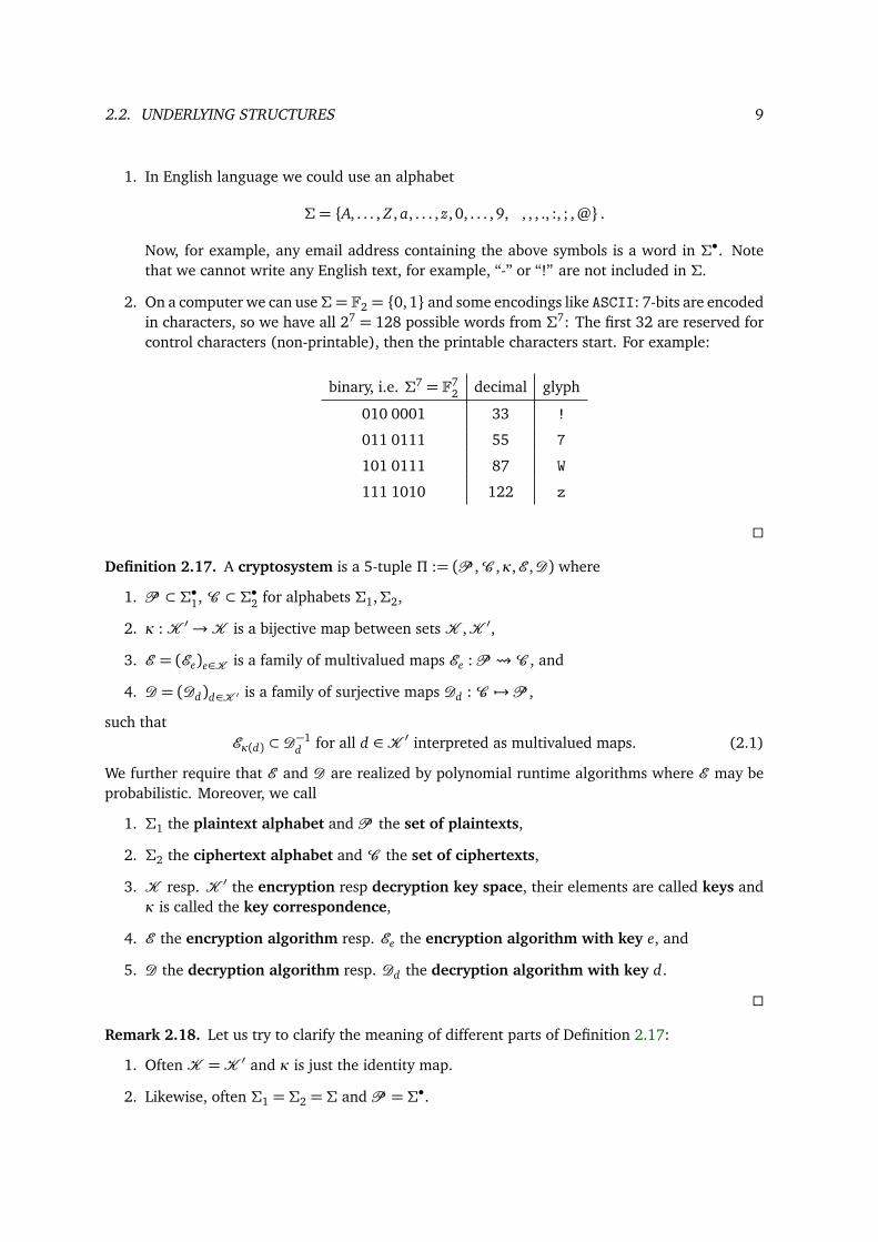
2. On a computer we can useΣ= F2 = 0, 1 and some encodings like ASCII: 7-bits are encodedin characters, so we have all 27 = 128 possible words from Σ7: The first 32 are reserved forcontrol characters (non-printable), then the printable characters start. For example:
binary, i.e. Σ7 = F72 decimal glyph
010 0001 33 !
011 0111 55 7
101 0111 87 W
111 1010 122 z
Definition 2.17. A cryptosystem is a 5-tuple Π := (P ,C ,κ,E ,D) where
1. P ⊂ Σ•1, C ⊂ Σ•2 for alphabets Σ1,Σ2,
2. κ :K ′→K is a bijective map between sets K ,K ′,3. E = (Ee)e∈K is a family of multivalued maps Ee :P C , and
4. D = (Dd)d∈K ′ is a family of surjective maps Dd :C 7→ P ,
such thatEκ(d) ⊂ D−1
d for all d ∈K ′ interpreted as multivalued maps. (2.1)
We further require that E and D are realized by polynomial runtime algorithms where E may beprobabilistic. Moreover, we call
1. Σ1 the plaintext alphabet and P the set of plaintexts,
2. Σ2 the ciphertext alphabet and C the set of ciphertexts,
3. K resp. K ′ the encryption resp decryption key space, their elements are called keys andκ is called the key correspondence,
4. E the encryption algorithm resp. Ee the encryption algorithm with key e, and
5. D the decryption algorithm resp. Dd the decryption algorithm with key d.
Remark 2.18. Let us try to clarify the meaning of different parts of Definition 2.17:
1. Often K =K ′ and κ is just the identity map.
2. Likewise, often Σ1 = Σ2 = Σ and P = Σ•.
10 CHAPTER 2. BASIC CONCEPTS
3. Ee being a multivalued map is no problem as long as Equation 2.1 holds. It ensures that evenif the encryption leads to a set of ciphertexts this set is in the preimage of correspondingdecryption algorithm. Moreover, it follows that the multivalued map Ee is injective for alle ∈K .
4. In particular, we often assume that both, E and D, are families of maps, in particular, E is afamily of injective maps P →C . Moreover, it then holds by construction that
∀d ∈K ′ Eκ(d) Dd = idC ,∀e ∈K Dκ−1(e) Ee = idP .
Example 2.19. Recall Example 1.1:
1. We can describe Caesar’s cryptosystem via
Σ1 = Σ2 = Σ=P =C =K =K ′ = A, . . . , Z ∼= Z/26Z, and
Ek : P → C , m 7→ (m+ k) mod 26,Dℓ : C → P , c 7→ (c − ℓ) mod 26.
In other words: Ek = D−k and thus Ek is a map for all k ∈K .
2. The Vigenère cryptosystem now generalizes the Caesar one to: We still have Σ1 = Σ2 = Σ∼=Z/26Z and K =K ′, but now P =C =K = Σ|k| for a key k. In our example we have
k = “SECRET”= (18, 4, 2, 17, 4, 19) ∈ (Z/26Z)6 .
Thus we can assume P ,C ⊂ Σ6 (if the texts are longer we can cut them in blocks of length6) and we can apply E and D component wise:
Ek : P → C , m 7→ (m+ k) mod 26 = (m1 + k1, . . . , m6 + k6) mod 26,Dℓ : C → P , c 7→ (c − ℓ) mod 26 = (c1 − ℓ1, . . . , c6 − ℓ6) mod 26.
Again it holds that Ek = D−k and thus Ek is a map for all k ∈K .
Definition 2.20. A cipher7 is an algorithm for performing encryption or decryption. If we have acryptosystem, the corresponding cipher is given by E resp. D (implicitly also the keyspaces K orK ′ resp. κ). In the following we use the terms cryptosystem and cipher synonymously to eachother.
There are two main categories of ciphers in terms of key handling: If κ is feasible then K andK ′ need to be kept secret and the cipher is called symmetric. Otherwise the cipher is calledasymmetric. We also call a cryptosystem symmetric resp. asymmetric if its corresponding cipheris symmetric resp. asymmetric. An asymmetric cryptosystem is also called a public key cryp-tosystem as K can be made public without weakening the secrecy of the “private” key set K ′ fordecryption. The elements of K are then called public keys, those of K ′ are called private keys.
7Some authors also write cypher, in German it stands for Chiffre.
2.3. INVESTIGATING SECURITY MODELS 11
Remark 2.21. Implementations of symmetric cryptosystems are more efficient than those of asym-metric cryptosystems. Thus, asymmetric ciphers are in general only used for exchanging the neededprivate keys in order to start a secure communication via a symmetric cipher.
Example 2.22. Both, Ceasar’s and Vigenère’s cryptosystem, are symmetric ones as encryption bythe key k is decrypted with the key −k.
In the early days of cryptography the systems resp. ciphers were kept secret.8 Doing so is no longerpossible nowadays and also has the disadvantage that no research on the security of a cryptosystemkept secret can be done. Thus, the following principle is widely accepted in cryptology:
Principle 2.23 (Kerckhoff, 1883). The cryptographic strength of a cryptosystem should not dependon the secrecy of the cryptosystem, but only on the secrecy of the decryption key.
In other words: The attacker always knows the cryptosystem.
2.3 Investigating Security Models
Definition 2.24. For a given cryptosystem Π we define the following security properties:
1. Π has onewayness (OW) if it is infeasbile for an attacker to decrypt an arbitrary ciphertext.
2. Π has indistinguishability (IND) if it is infeasible for an attacker to associate a given cipher-text to one of several known plaintexts.
3. Π has non-malleability (NM) if it is infeasible for an attacker to modify a given ciphertext ina way such that the corresponding plain text is sensible in the given language resp. context.
Remark 2.25. It is known that NM⇒ IND⇒ OW.
Definition 2.26.
1. An active attack on a cryptosystem is one in which the attacker actively changes the com-munication by, for example, creating, altering, replacing or blocking messages.
2. A passive attack on a cryptosystem is one in which the attacker only eavesdrops plaintextsand ciphertexts. In contrast to an active attack the attacker cannot alter any messages she/hesees.
In this lecture we are mostly interested in passive attacks. Some attack scenarios we might considerare presented in the following:
Definition 2.27.
1. The attacker receives only ciphertexts: ciphertext-only attack (COA).
8Security by obscurity.
12 CHAPTER 2. BASIC CONCEPTS
2. The attacker receives pairs of plaintexts and corresponding ciphertexts: known-plaintextattack (KPA).
3. The attacker can for one time choose a plaintext and receives the corresponding ciphertext.He cannot alter his choice depending on what he receives: chosen-plaintext attack (CPA).
4. The attacker is able to adaptively choose ciphertexts and to receive the corresponding plain-texts. The attacker is allowed to alter the choice depending on what is received. So theattacker has access to the decryption cipher Dd and wants to get to know the decryption keyd: adaptive chosen-ciphertext attack (CCA).
Remark 2.28. In a public cryptosystem CPA is trivial. Moreover, one can show that in general itholds that
CCA> CPA> KPA> COA.
Definition 2.29. A security model is a security property together with an attack scenario.
Example 2.30. IND-CCA is a security model. One would check the indistinguishability of a givencryptosystem Π w.r.t. an adaptive chosen-ciphertext attack.
Chapter 3
Modes of Ciphers
For ciphers we have, in general, four different categories:
1. symmetric and asymmetric ciphers (see Definition 2.20), and
2. stream and block ciphers.
In the following we often assume binary representation of symbols, i.e. we are working with bitsin Z/2Z. All of what we are doing can be easily generalized to other representations and otheralphabets.
3.1 Block Ciphers
Definition 3.1. Let Σ be an alphabet. A block cipher is a cipher acting onP =C = Σn for a givenblock size n ∈ N. Block ciphers with block size n= 1 are called substitution ciphers.
Lemma 3.2. The encryption functions of block ciphers are the permutations on Σn.
Proof. By definition the encryption functions Ee are injective for each e ∈ K . Injective functionsEe : Σn→ Σn are bijective, thus permutations on Σn.
If we assume P = C = Σn the keyspace K ′ = K = S (Σn) is the set of all permutations on Σn.Depending on Σ and n, S (Σn) is huge, having (|Σ|n)! elements. In practice one chooses only asubset of S (Σn) such that the permutations can be generated easily by short keys. Clearly, thismight install a security problem to the cryptosystem.
A special case of this restriction is to use the permutation group Sn on the positions as key space:
Example 3.3. A permutation cipher is a block cipher that works on P =C = Σn for some n ∈ Nand uses K ′ =K = Sn. In this way |K ′|= n! which is much smaller than |S (Σn) |. Let π ∈K :
Eπ : Σn→ Σn, (v1, . . . , vn) 7→vπ(1), . . . , vπ(n)
,Dπ−1 : Σn→ Σn, (v1, . . . , vn) 7→
vπ−1(1), . . . , vπ−1(n)
.
For example, let n= 3 and Σ= Z/2Z. We use the keyspaces
K ′ =K = S3 = (1), (1 2), (1 3), (23), (123), (13 2)13
14 CHAPTER 3. MODES OF CIPHERS
with 3! elements. Now we could, for example, encrypt the plaintext (v1, v2, v3) = (1, 0, 1) ∈ Σ3 viaπ= (123): Eπ ((1, 0, 1)) = (v2, v3, v1) = (0, 1, 1).
For a symmetric block cipher one can increase the level of security to multiple applications of thethe cipher:
Remark 3.4. Let E and D represent a symmetric block cipher of block size n, w.l.o.g. we assumeK ′ = K . An easy way to increase its security is to apply the so-called triple encryption: Takethree keys k1, k2, k3 ∈K . Then one can encrypt a plaintext p ∈ P via
Ek3
Dk2
Ek1(p)=: c ∈ C .
There are three different settings for the keys:
1. If k1 = k2 = k3 the above encryption is equivalent to Ek1(p).
2. If k1 = k3 and k2 is different, then the key size is doubled to 2 · n.
3. If all three keys are different the key size tripled to 3 · n.1
So why not applying 100 keys to increase security? The problem is the increasing time for encryp-tion and decryption that makes it no longer practical at some point.
Clearly, if the encryption functions itself would generate a (small) group then applying the en-cryption resp. decryption several times would not give any advantage in terms of security. Forexample, take the data encryption standard (DES) encryption function (cf. Section 6.2): It has256 encryption functions, for each 56 bit key one. Still, we have
256!
possible permutations.It is shown by Campell and Wiener that the set of DES encryption functions is not closed undercomposition, i.e., they do not build a group. In other words, there exist keys k1 and k2 such thatDESk2
DESk1= DESk for all keys k. It follows that the number of permutations of the form
DESk2DESk1
is much larger than the number of permutations of type DESk.
Until now we always considered that our plaintexts have the same size as the key. Clearly, in gen-eral, one wants to encrypt longer documents or texts. For this problem there are several differentmodes one can apply block ciphers.
3.2 Modes of Block Ciphers
Let us assume in this section that Σ= Z/2Z, block size is n ∈ N>0 and the key spacesK ′ =K arethe same. We switch between representations of plaintexts: For example let n = 3, then we canidentify all natural numbers between 0 and 7. So we can represent 0 binary as 000 or (0, 0, 0) ∈(Z/2Z)3, or 5 as 101 or (1, 0, 1).
We further assume that there is some magic that randomly resp. pseudo randomly and uniformlydistributed chooses a key k ∈K .2
1 The idea of applying three different keys and not only two comes from the so-called meet-in-the-middle attackswhich allows attacking two key encryptions with nearly the same runtime as one key encryption (but with a bigger spacecomplexity.
2More on randomness later, here we keep it simple and out of our way.
3.2. MODES OF BLOCK CIPHERS 15
Assume we have a plaintext p ∈ P of arbitrary but finite length. We divide p into blocks of lengthn. If the length of p is not divisible by n then we add some random symbols at the end of p. In theend we receive a repesentation p = (p1, . . . , pm) where all pi are plaintext blocks of length n.
Each plaintext block pi is encrypted to a corresponding ciphertext block ci using a given key k. Inthe end, the ciphertext corresponding to p = (p1, . . . , pm) is c = (c1, . . . , cm). The fitting decryptionprocess works exactly the same way: One takes each block ci and applies the decryption functionD with the fitting key k′ for k in order to receive the plaintext block pi .
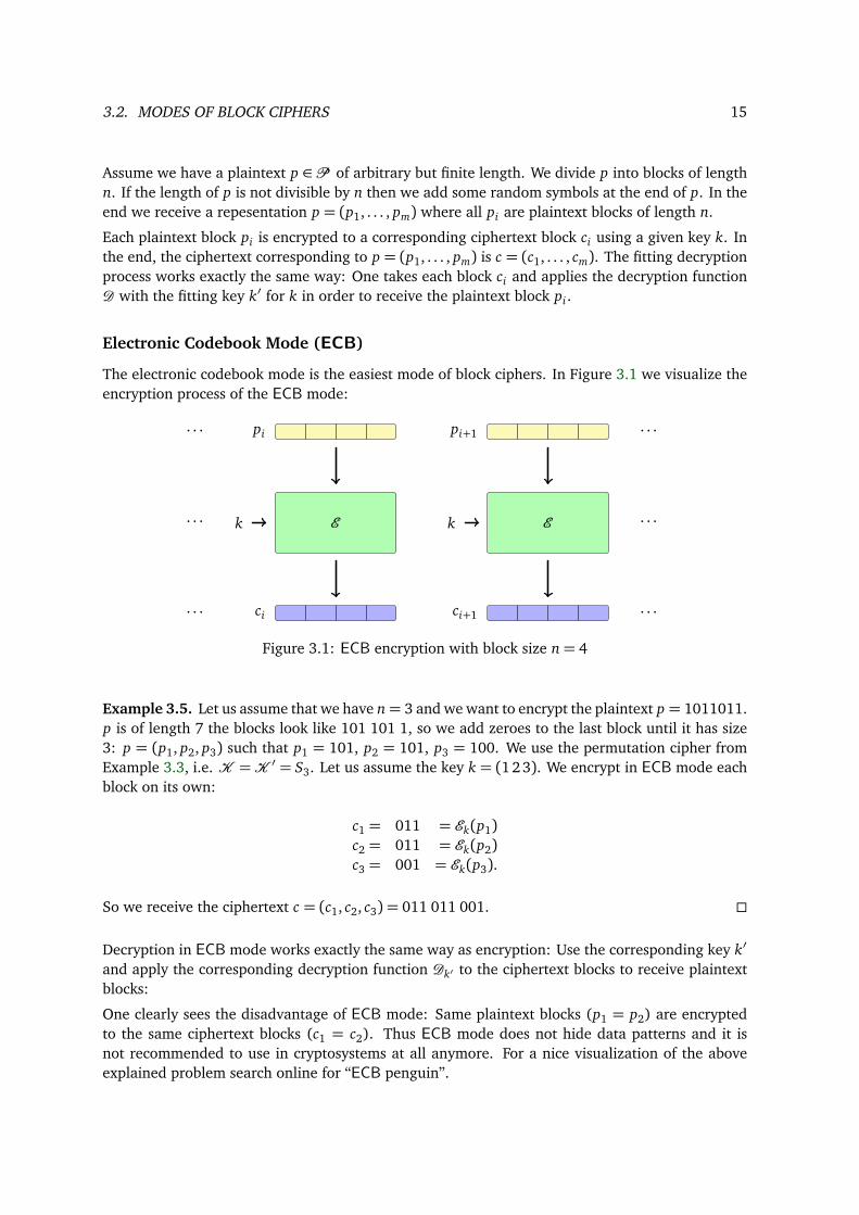
Electronic Codebook Mode (ECB)
The electronic codebook mode is the easiest mode of block ciphers. In Figure 3.1 we visualize theencryption process of the ECB mode:
pi
ci
pi+1
ci+1
k E k E
· · ·
· · ·
· · ·
· · ·
· · ·
· · ·
Figure 3.1: ECB encryption with block size n= 4
Example 3.5. Let us assume that we have n= 3 and we want to encrypt the plaintext p = 1011011.p is of length 7 the blocks look like 101 101 1, so we add zeroes to the last block until it has size3: p = (p1, p2, p3) such that p1 = 101, p2 = 101, p3 = 100. We use the permutation cipher fromExample 3.3, i.e. K =K ′ = S3. Let us assume the key k = (123). We encrypt in ECB mode eachblock on its own:
c1 = 011 = Ek(p1)c2 = 011 = Ek(p2)c3 = 001 = Ek(p3).
So we receive the ciphertext c = (c1, c2, c3) = 011 011 001.
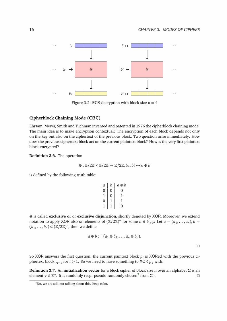
Decryption in ECB mode works exactly the same way as encryption: Use the corresponding key k′and apply the corresponding decryption function Dk′ to the ciphertext blocks to receive plaintextblocks:
One clearly sees the disadvantage of ECB mode: Same plaintext blocks (p1 = p2) are encryptedto the same ciphertext blocks (c1 = c2). Thus ECB mode does not hide data patterns and it isnot recommended to use in cryptosystems at all anymore. For a nice visualization of the aboveexplained problem search online for “ECB penguin”.
16 CHAPTER 3. MODES OF CIPHERS
ci
pi
ci+1
pi+1
k′ D k′ D
· · ·
· · ·
· · ·
· · ·
· · ·
· · ·
Figure 3.2: ECB decryption with block size n= 4
Cipherblock Chaining Mode (CBC)
Ehrsam, Meyer, Smith and Tuchman invented and patented in 1976 the cipherblock chaining mode.The main idea is to make encryption contextual: The encryption of each block depends not onlyon the key but also on the ciphertext of the previous block. Two question arise immediately: Howdoes the previous ciphertext block act on the current plaintext block? How is the very first plaintextblock encrypted?
Definition 3.6. The operation
⊕ : Z/2Z×Z/2Z→ Z/2Z, (a, b) 7→ a⊕ b
is defined by the following truth table:
a b a⊕ b0 0 01 0 10 1 11 1 0
⊕ is called exclusive or or exclusive disjunction, shortly denoted by XOR. Moreover, we extendnotation to apply XOR also on elements of (Z/2Z)n for some n ∈ N>0: Let a = (a1, . . . , an), b =(b1, . . . , bn) ∈ (Z/2Z)n, then we define
a⊕ b := (a1 ⊕ b1, . . . , an ⊕ bn).
So XOR answers the first question, the current paintext block pi is XORed with the previous ci-phertext block ci−1 for i > 1. So we need to have something to XOR p1 with:
Definition 3.7. An initialization vector for a block cipher of block size n over an alphabet Σ is anelement v ∈ Σn. It is randomly resp. pseudo randomly chosen3 from Σn.
3No, we are still not talking about this. Keep calm.
3.2. MODES OF BLOCK CIPHERS 17
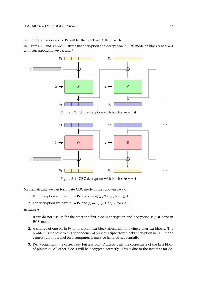
So the initialization vector IV will be the block we XOR p1 with.
In Figures 3.3 and 3.4 we illustrate the encryption and decryption in CBC mode on block size n= 4with corresponding keys k and k′.
IV
p1
c1
p2
c2
k E k E
· · ·
· · ·Figure 3.3: CBC encryption with block size n= 4
IV
c1
p1
c2
p2
k′ D k′ D
· · ·
· · ·Figure 3.4: CBC decryption with block size n= 4
Mathematically we can formulate CBC mode in the following way:
1. For encryption we have co = IV and ci = Ek(pi ⊕ ci−1) for i ≥ 1.
2. For decryption we have co = IV and pi = Dk′(ci)⊕ ci−1 for i ≥ 1.
Remark 3.8.
1. If we do not use IV for the start the first block’s encryption and decryption is just done inECB mode.
2. A change of one bit in IV or in a plaintext block affects all following ciphertext blocks. Theproblem is that due to this dependency of previous ciphertext blocks encryption in CBC modecannot run in parallel on a computer, it must be handled sequentially.
3. Decrypting with the correct key but a wrong IV affects only the correctness of the first blockof plaintext. All other blocks will be decrypted correctly. This is due to the fact that for de-
18 CHAPTER 3. MODES OF CIPHERS
cryption we only need the previous ciphertext block, but not the decrypted previous plaintextblock. It follows that decryption in CBC mode can be done in parallel.
4. Changing one bit in a ciphertext block causes complete corruption of the corresponding plain-text block, and inverts the corresponding bit in the following plaintext block. All other blocksstay correct. This fact is used by several attacks on this mode, see, for example, [Wik16e]
5. In order to make such attacks more difficult there is also a variant of CBC called PCBC: thepropagating cipherblock chaining mode. which also takes the previous plaintext block intoaccount when encrypting resp. decrypting the current plaintext block.
Example 3.9. Let us recall Example 3.5: n = 3, p = 101 101 100 and k = (12 3). We chooseIV= 101.
c1 = 000 = Ek(p1 ⊕ IV)c2 = 011 = Ek(p2 ⊕ c1)c3 = 111 = Ek(p3 ⊕ c2).
So we receive the ciphertext c = (c1, c2, c3) = 000 011 111. We see that in CBC mode c1 = c2whereas p1 = p2.
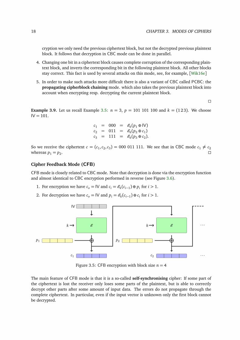
Cipher Feedback Mode (CFB)
CFB mode is closely related to CBC mode. Note that decryption is done via the encryption functionand almost identical to CBC encryption performed in reverse (see Figure 3.6).
1. For encryption we have co = IV and ci = Ek(ci−1)⊕ pi for i > 1.
2. For decryption we have co = IV and pi = Ek(ci−1)⊕ ci for i > 1.
p1 p2
IV
c1 c2
k E k E · · ·
· · ·Figure 3.5: CFB encryption with block size n= 4
The main feature of CFB mode is that it is a so-called self-synchronising cipher: If some part ofthe ciphertext is lost the receiver only loses some parts of the plaintext, but is able to correctlydecrypt other parts after some amount of input data. The errors do not propagate through thecomplete ciphertext. In particular, even if the input vector is unknown only the first block cannotbe decrypted.
3.2. MODES OF BLOCK CIPHERS 19
c1 c2
IV
p1 p2
k E k E · · ·
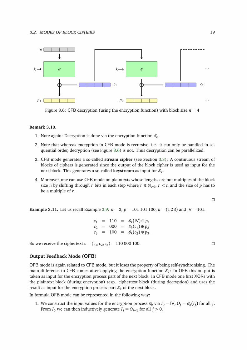
· · ·Figure 3.6: CFB decryption (using the encryption function) with block size n= 4
Remark 3.10.
1. Note again: Decryption is done via the encryption function Ek.
2. Note that whereas encryption in CFB mode is recursive, i.e. it can only be handled in se-quential order, decryption (see Figure 3.6) is not. Thus decryption can be parallelized.
3. CFB mode generates a so-called stream cipher (see Section 3.3): A continuous stream ofblocks of ciphers is generated since the output of the block cipher is used as input for thenext block. This generates a so-called keystream as input for Ek.
4. Moreover, one can use CFB mode on plaintexts whose lengths are not multiples of the blocksize n by shifting through r bits in each step where r ∈ N>0, r < n and the size of p has tobe a multiple of r.
Example 3.11. Let us recall Example 3.9: n= 3, p = 101 101 100, k = (123) and IV= 101.
c1 = 110 = Ek(IV)⊕ p1c2 = 000 = Ek(c1)⊕ p2c3 = 100 = Ek(c2)⊕ p3.
So we receive the ciphertext c = (c1, c2, c3) = 110 000 100.
Output Feedback Mode (OFB)
OFB mode is again related to CFB mode, but it loses the property of being self-synchronising. Themain difference to CFB comes after applying the encryption function Ek: In OFB this output istaken as input for the encryption process part of the next block. In CFB mode one first XORs withthe plaintext block (during encryption) resp. ciphertext block (during decryption) and uses theresult as input for the encryption process part Ek of the next block.
In formula OFB mode can be represented in the following way:
1. We construct the input values for the encryption process Ek via I0 = IV, Oj = Ek(I j) for all j.From I0 we can then inductively generate I j = Oj−1 for all j > 0.
20 CHAPTER 3. MODES OF CIPHERS
p1 p2
IV
c1 c2
k E k E · · ·
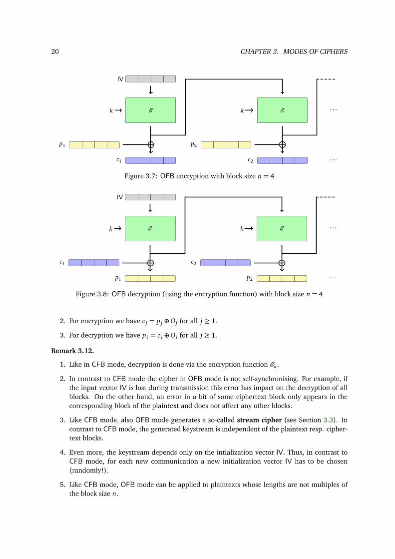
· · ·Figure 3.7: OFB encryption with block size n= 4
c1 c2
IV
p1 p2
k E k E · · ·
· · ·Figure 3.8: OFB decryption (using the encryption function) with block size n= 4
2. For encryption we have c j = p j ⊕Oj for all j ≥ 1.
3. For decryption we have p j = c j ⊕Oj for all j ≥ 1.
Remark 3.12.
1. Like in CFB mode, decryption is done via the encryption function Ek.
2. In contrast to CFB mode the cipher in OFB mode is not self-synchronising. For example, ifthe input vector IV is lost during transmission this error has impact on the decryption of allblocks. On the other hand, an error in a bit of some ciphertext block only appears in thecorresponding block of the plaintext and does not affect any other blocks.
3. Like CFB mode, also OFB mode generates a so-called stream cipher (see Section 3.3). Incontrast to CFB mode, the generated keystream is independent of the plaintext resp. cipher-text blocks.
4. Even more, the keystream depends only on the intialization vector IV. Thus, in contrast toCFB mode, for each new communication a new initialization vector IV has to be chosen(randomly!).
5. Like CFB mode, OFB mode can be applied to plaintexts whose lengths are not multiples ofthe block size n.
3.2. MODES OF BLOCK CIPHERS 21
6. In OFB mode one can parallelize encryption and decryption partly: The idea is to first takethe initialization vector IV and apply to it Ek. This is the input of the application of Ek forthe next block. So one can sequentially precompute all these intermediate blocks, and thenXOR them, in parallel, with the corresponding plaintext block (when encrypting) resp. thecorresponding ciphertext block (when decrypting).
7. By construction, the first ciphertext block in CFB and OFB mode is encrypted equivalently.
Example 3.13. Let us recall Example 3.11: n= 3, p = 101 101 100, k = (123) and IV= 101.
O1 = 011 = Ek(IV)O2 = 110 = Ek(O1)O3 = 101 = Ek(O2)c1 = 110 = O1 ⊕ p1c2 = 011 = O2 ⊕ p2c3 = 001 = O3 ⊕ p3.
So we receive the ciphertext c = (c1, c2, c3) = 110 011 001.
Counter Mode (CTR)
CTR mode is different from CBC, CFB and OFB in the sense that instead of an initialization vectorit uses a so-called nonce:
Definition 3.14. A nonce is an arbitrary number used only once for cryptographic communication.They are often pseudo random resp. random numbers.4
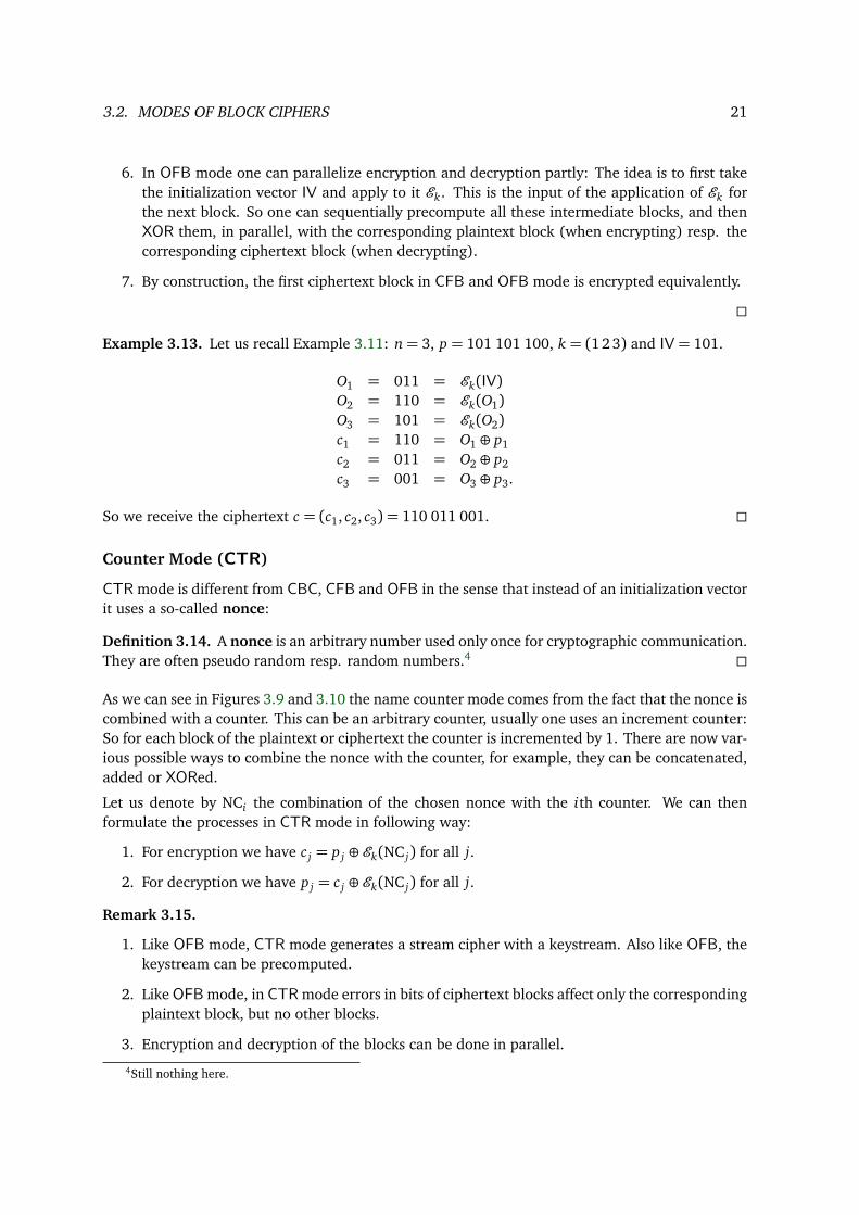
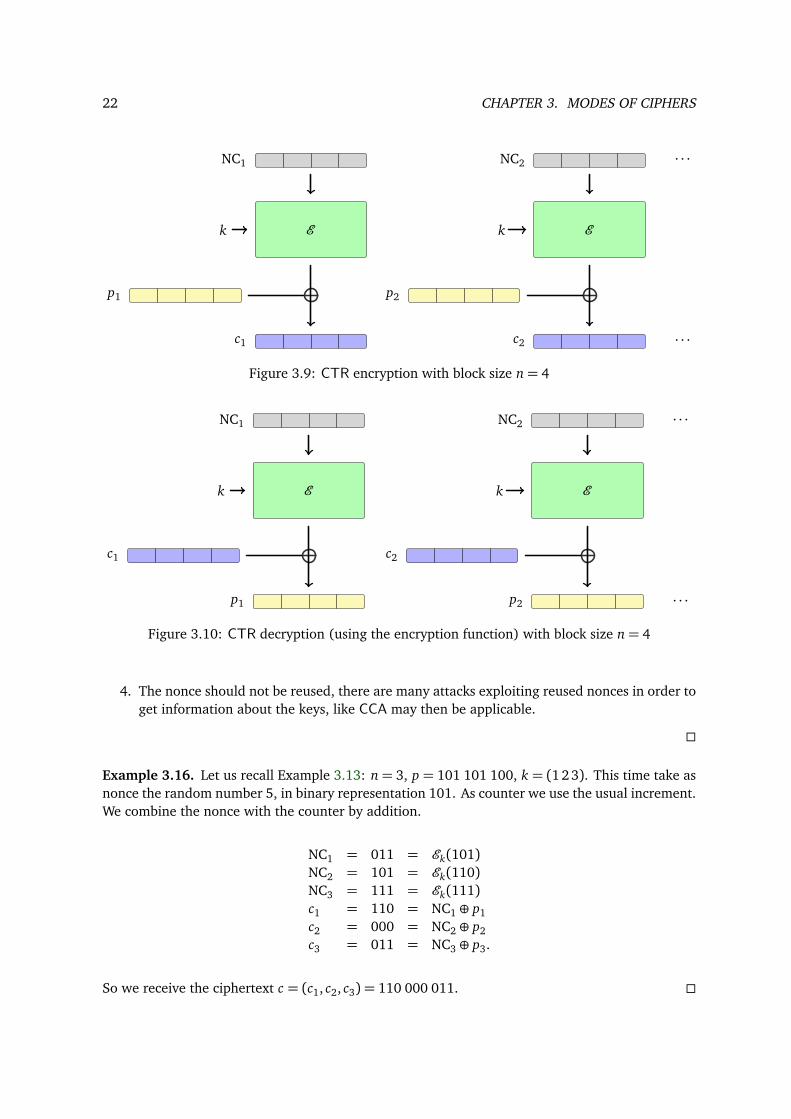
As we can see in Figures 3.9 and 3.10 the name counter mode comes from the fact that the nonce iscombined with a counter. This can be an arbitrary counter, usually one uses an increment counter:So for each block of the plaintext or ciphertext the counter is incremented by 1. There are now var-ious possible ways to combine the nonce with the counter, for example, they can be concatenated,added or XORed.
Let us denote by NCi the combination of the chosen nonce with the ith counter. We can thenformulate the processes in CTR mode in following way:
1. For encryption we have c j = p j ⊕Ek(NC j) for all j.
2. For decryption we have p j = c j ⊕Ek(NC j) for all j.
Remark 3.15.
1. Like OFB mode, CTR mode generates a stream cipher with a keystream. Also like OFB, thekeystream can be precomputed.
2. Like OFB mode, in CTR mode errors in bits of ciphertext blocks affect only the correspondingplaintext block, but no other blocks.
3. Encryption and decryption of the blocks can be done in parallel.
4Still nothing here.
22 CHAPTER 3. MODES OF CIPHERS
p1
NC1
c1
k E
p2
NC2
c2
k E
· · ·
· · ·Figure 3.9: CTR encryption with block size n= 4
c1
NC1
p1
k E
c2
NC2
p2
k E
· · ·
· · ·Figure 3.10: CTR decryption (using the encryption function) with block size n= 4
4. The nonce should not be reused, there are many attacks exploiting reused nonces in order toget information about the keys, like CCA may then be applicable.
Example 3.16. Let us recall Example 3.13: n= 3, p = 101 101 100, k = (12 3). This time take asnonce the random number 5, in binary representation 101. As counter we use the usual increment.We combine the nonce with the counter by addition.
NC1 = 011 = Ek(101)NC2 = 101 = Ek(110)NC3 = 111 = Ek(111)c1 = 110 = NC1 ⊕ p1c2 = 000 = NC2 ⊕ p2c3 = 011 = NC3 ⊕ p3.
So we receive the ciphertext c = (c1, c2, c3) = 110 000 011.
3.3. STREAM CIPHERS 23
Note that until now we are only thinking about encryption and decryption. The above modes canalso be combined with authentication procedures. For example, CTR mode together with authen-tication is known as Galois Counter mode (GCM). Its name comes from the fact that the authen-tication function is just a multiplication in the Galois field GF(2k) for some k ∈ N. For example, theAES cryptosystem (see Section 6.3) uses k = 128 by default. We will discuss authentication lateron, for example, see Chapter 13.
Nowadays, CBC and CTR mode are widely accepted in the crypto community. For example, theyare used in encrypted ZIP archives (also in other archiving tools), CTR is used in TLS 1.25 in yourweb browser or for off-the-record messaging (OTR)6 in your messaging app (usually in combina-tion with AES).
3.3 Stream Ciphers
In contrast to block ciphers, stream ciphers can handle plaintexts resp. ciphertext of any sizewithout the necessity of having blocks.
Definition 3.17. Let Σ be an alphabet.
1. A keystream is a stream of random or pseudo random7 characters or digits from Σ that arecombined with a plaintext (ciphertext) digit in order to produce a ciphertext (plaintext) digit.
2. A stream cipher is a symmetric cipher acting on plaintexts and ciphertexts P ,C ⊂ Σ• ofany given length. Each plaintext digit (e.g. binary representation) is encrypted one at a timewith a corresponding digit of a keystream.
3. A stream cipher is called synchronous if the keystream is independent of the plaintext andthe ciphertext.
4. A stream cipher is called self-synchronizing if the keystream is computed depending on then previous ciphertext digits for some n ∈ N>0.
Example 3.18. CFB mode and OFB mode are examples of stream ciphers. CFB is self-synchronizingwhereas OFB is synchronous.
Remark 3.19.
1. In practice a digit is usually a bit (binary representation) and the combination is just XOR.
2. Self-synchronizing stream ciphers have the advantage that if some ciphertext digits are lost orcorrupted during transmission this error will not propagate to all following ciphertext digitsbut only to the next n ones. In a synchronous stream cipher one cannot recover a ciphertextdigit lost or added during transmission, the complete following decryption may fail.
5TLS stands for Transport Layer Security. It is a protocol that provides private resp. encrypted communication,
authentication and integrity for a lot of applications like web browsing, emails, messaging, voice-over-IP, etc.6OTR provides deniable authentication, i.e. after an encrypted communication no one can ensure that a given
encryption key was used by a chosen person.7We really will come to this topic soon!
24 CHAPTER 3. MODES OF CIPHERS
Binary stream ciphers are usually implemented using so-called linear feedback shift registers:
Definition 3.20. Let Σ = Z/2Z, P ,C ⊂ Σ•, K ′ = K = Σn for some n ∈ N>0. Let IV ∈ Σn bean initialization vector. Assume a plaintext p = p1 . . . pm of some size m in Σ•. The keystreamk = k1k2k3 . . . is initialized via
ki = IVi for all 1≤ i ≤ n.
A linear feedback shift register (LFSR) is a shift register used for generating pseudo random bits.Its input bit is a linear function f of its previous state. For j > 0 one now generates
k j+n = f (k j , . . . , k j+n−1).
Encryption is now done via Ek(p) = p1⊕ k1 . . . , pm⊕ km = c, Analogously, decryption is performedwith Dk(c) = c1 ⊕ k1, . . . , cm ⊕ km = p.
In general, this linear function is XOR resp. a combination of several XORs.
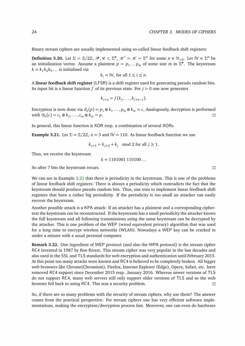
Example 3.21. Let Σ= Z/2Z, n= 3 and IV= 110. As linear feedback function we use
k j+3 = k j+2 + k j mod 2 for all j ≥ 1.
Thus, we receive the keystreamk = 1101001 110100 . . .
So after 7 bits the keystream recurs.
We can see in Example 3.21 that there is periodicity in the keystream. This is one of the problemsof linear feedback shift registers: There is always a periodicity which contradicts the fact that thekeystream should produce pseudo random bits. Thus, one tries to implement linear feedback shiftregisters that have a rather big periodicity. If the periodicity is too small an attacker can easilyrecover the keystream.
Another possible attack is a KPA attack: If an attacker has a plaintext and a corresponding cipher-text the keystream can be reconstructed. If the keystream has a small periodicity the attacker knowsthe full keystream and all following transmissions using the same keystream can be decrypted bythe attacker. This is one problem of the WEP (wired equivalent privacy) algorithm that was usedfor a long time to encrypt wireless networks (WLAN). Nowadays a WEP key can be cracked inunder a minute with a usual personal computer.
Remark 3.22. One ingredient of WEP protocol (and also the WPA protocol) is the stream cipherRC4 invented in 1987 by Ron Rivest. This stream cipher was very popular in the last decades andalso used in the SSL and TLS standards for web encryption and authentication until February 2015.At this point too many attacks were known and RC4 is believed to be completely broken. All biggerweb browsers like Chrome(Chromium), Firefox, Internet Explorer (Edge), Opera, Safari, etc. haveremoved RC4 support since December 2015 resp. January 2016. Whereas newer versions of TLSdo not support RC4, many web servers still only support older versions of TLS and so the webbrowser fell back to using RC4. This was a security problem.
So, if there are so many problems with the security of stream ciphers, why use them? The answercomes from the practical perspective: For stream ciphers one has very efficient software imple-mentations, making the encryption/decryption process fast. Moreover, one can even do hardware
3.4. A SHORT REVIEW OF HISTORICAL CIPHERS 25
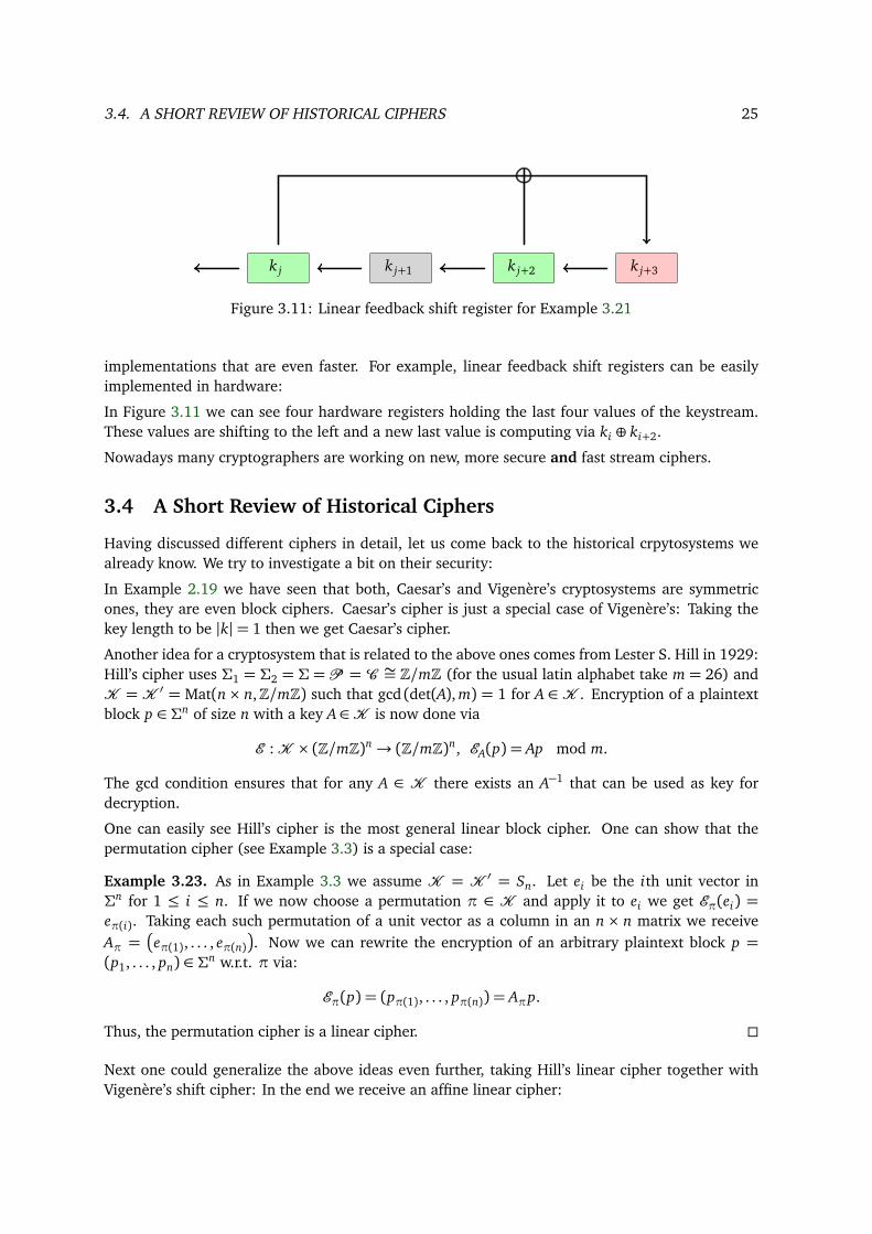
k j k j+1 k j+2 k j+3
Figure 3.11: Linear feedback shift register for Example 3.21
implementations that are even faster. For example, linear feedback shift registers can be easilyimplemented in hardware:
In Figure 3.11 we can see four hardware registers holding the last four values of the keystream.These values are shifting to the left and a new last value is computing via ki ⊕ ki+2.
Nowadays many cryptographers are working on new, more secure and fast stream ciphers.
3.4 A Short Review of Historical Ciphers
Having discussed different ciphers in detail, let us come back to the historical crpytosystems wealready know. We try to investigate a bit on their security:
In Example 2.19 we have seen that both, Caesar’s and Vigenère’s cryptosystems are symmetricones, they are even block ciphers. Caesar’s cipher is just a special case of Vigenère’s: Taking thekey length to be |k|= 1 then we get Caesar’s cipher.
Another idea for a cryptosystem that is related to the above ones comes from Lester S. Hill in 1929:Hill’s cipher uses Σ1 = Σ2 = Σ = P = C ∼= Z/mZ (for the usual latin alphabet take m = 26) andK = K ′ = Mat(n× n,Z/mZ) such that gcd (det(A), m) = 1 for A ∈ K . Encryption of a plaintextblock p ∈ Σn of size n with a key A∈K is now done via
E :K × (Z/mZ)n→ (Z/mZ)n, EA(p) = Ap mod m.
The gcd condition ensures that for any A ∈ K there exists an A−1 that can be used as key fordecryption.
One can easily see Hill’s cipher is the most general linear block cipher. One can show that thepermutation cipher (see Example 3.3) is a special case:
Example 3.23. As in Example 3.3 we assume K = K ′ = Sn. Let ei be the ith unit vector inΣn for 1 ≤ i ≤ n. If we now choose a permutation π ∈ K and apply it to ei we get Eπ(ei) =eπ(i). Taking each such permutation of a unit vector as a column in an n × n matrix we receiveAπ =eπ(1), . . . , eπ(n). Now we can rewrite the encryption of an arbitrary plaintext block p =
(p1, . . . , pn) ∈ Σn w.r.t. π via:
Eπ(p) = (pπ(1), . . . , pπ(n)) = Aπp.
Thus, the permutation cipher is a linear cipher.
Next one could generalize the above ideas even further, taking Hill’s linear cipher together withVigenère’s shift cipher: In the end we receive an affine linear cipher:
26 CHAPTER 3. MODES OF CIPHERS
Definition 3.24. Let Σ = Z/mZ for some m ∈ N>0, let P = C = Σn for n ∈ N>0. Moreover, letK = K ′ = Mat (n× n,Σ)×Σn such that for k = (A, b) ∈ K it holds that gcd (det(A), m) = 1. Anaffine linear block cipher is then defined by the encryption function Ek where k = (A, b) appliedto the plaintext block p = (p1, . . . , pn) ∈ Σn such that
Ek : Σn→ Σn, p 7→ Ap+ b mod m.
The corresponding decryption with k′ = (A−1, b) is done via
Dk′ : Σn→ Σn, c 7→ A−1(c − b) mod m.
Clearly, all other considered ciphers are affine linear ciphers:
1. For Caesar’s cipher take n= 1, K =K ′ = En ×Σ where En is the identity matrix.
2. For Vigenère’s cipher take n ∈ N>0, K =K ′ = En ×Σ.
3. For Hill’s cipher take n ∈ N>0, K =K ′ =Mat (n× n,Σ)× 0.Let us finish this section by trying to understand why all these ciphers based on affine linear func-tions are broken nowadays:
We assume an arbitrary affine linear cipher with Σ = Z/mZ for some m ∈ N>0, let P = C = Σn
for n ∈ N>0. Moreover, let K = K ′ = Mat (n× n,Σ)× Σn such that for k = (A, b) ∈ K it holdsthat gcd (det(A), m) = 1. Encryption is then given via the encryption function Ek where k = (A, b)applied to a plaintext block p ∈ Σn such that
Ek : Σn→ Σn, p 7→ Ap+ b mod m.
We try to do a KPA, so the attacker has n + 1 plaintext blocks p0, p1, . . . , pn ∈ Σn and the corre-sponding ciphertext blocks c0, c1, . . . , cn ∈ Σn. Then it holds that
ci − c0 ≡ A(pi − p0) mod m for all 1≤ i ≤ n. (3.1)
We construct two matrices:
1. Matrix P whose n columns are the differences pi − p0 mod m for 1≤ i ≤ n.
2. Matrix C whose n columns are the differences ci − c0 mod m for 1≤ i ≤ n.
Thus we can rewrite Equation 3.1 with matrices:
C ≡ AP mod m.
If gcd (det(P), m) = 1, we can compute P−1 and thus recover A:
A≡ C P−1 mod m.
Once we know A we can also recover b:
b ≡ c0 − Ap0 mod m.
Thus we have found the key k = (A, b). If the cipher is linear, i.e. b = 0 then one can set p0 = c0 =0 ∈ Σn and we can find A even with only n plaintext-ciphertext block pairs.
Chapter 4
Information Theory
In the last chapter we have seen that all affine linear ciphers are broken resp. not secure nowadays.Thus the question arises if there exist cryptosystems that are provable secure in a mathematicalsense. It turns out that this is possible.
4.1 A Short Introduction to Probability Theory
In order to discuss the security of a cryptosystem we need some basic knowledge of probabilitytheory.
Definition 4.1. Let Ω be a finite nonempty set and µ : Ω→ [0, 1] be a map with∑
x∈Ωµ(x) = 1.For A⊂ Ω we define µ(A) =
∑x∈Aµ(x).
1. µ is called a probability distribution.
2. The tuple (Ω,µ) is called a finite probability space.
3. A⊂ Ω is called an event, an element x ∈ Ω is called an elementary event.
4. The probability distribution µ defined by µ(x) := 1|Ω| is called the (discrete) uniform distri-
bution on Ω.
5. Let A, B ⊂ Ω such that µ(B)> 0. Then we define the conditional probability
µ(A|B) :=µ(A∩ B)µ(B)
.
That is, the probability of A given the occurence of B.
6. A, B ⊂ Ω are called (statistically) independent if
µ(A∩ B) = µ(A)µ(B).
Lemma 4.2. Let (Ω,µ) be a finite probability space and A, B ⊂ Ω be events.
1. µ(;) = 0, µ(Ω) = 1.
2. µ(Ω \ A) = 1−µ(A).27
28 CHAPTER 4. INFORMATION THEORY
3. If A⊂ B then µ(A)≤ µ(B).4. µ(A∩ B) = µ(A|B)µ(B).
Proof. All statements follow from Definition 4.1.
For the conditional probability there is the well-known formula by Thomas Bayes:
Theorem 4.3 (Bayes). Let (Ω,µ) be a finite probability space and A, B ⊂ Ω be two events such thatµ(A),µ(B)> 0. Then
µ(A|B) = µ(B|A)µ(A)µ(B)
.
Proof. By definition we have µ(A|B) = µ(A∩B)µ(B) and µ(B|A) = µ(A∩B)
µ(A) . Thus we conclude
µ(A|B)µ(B) = µ(A∩ B) = µ(B|A)µ(A).
Definition 4.4. Let (Ω,µ) be a finite probability space.
1. Let M be a set. A map X : Ω→ M is called an (M -valued discrete) random variable on Ω.
2. Let M be some set and let X be an M -valued random variable.
a) The distribution of X is defined by
µX (m) := µ(X = m) := µX−1(m)
for all m ∈ M .
More general, for A⊂ M we define
µX (A) := µ(X ∈ A) := µX−1(A)
.
b) X is called uniformly distributed if
µX (m) =1|M | for all m ∈ M .
3. If M ⊂ C and X is an M -valued random variable, then we define the expected value of X by
E(X ) :=∑x∈Ω
X (x)µ(x) ∈ C.
Moreover, let Y be another M -valued random variable. We define
X + Y : Ω→ C, (X + Y )(x) = X (x) + Y (x),X Y : Ω→ C, (X Y )(x) = X (x) · Y (x).
4. Let X i : Ω→ Mi be random variables for sets Mi for 1 ≤ i ≤ n. For mi ∈ Mi we define theproduct probability distribution
µX1,...,Xn(m1, . . . , mn) := µ(X1 = m1, . . . , Xn = mn) := µ
∩ni=1X i = mi
.
4.1. A SHORT INTRODUCTION TO PROBABILITY THEORY 29
Let X : Ω→ M and Y : Ω→ N be two random variables for sets M , N .
5. For µY (n)> 0 we define the conditional probability of X = m given the occurrence of Y = nby
µX |Y (m|n) :=µX ,Y (m, n)
µY (n).
6. X and Y are called (statistically) independent if
µX ,Y (m, n) = µX (m)µY (n) for all m ∈ M , n ∈ N .
The following properties are easily checked with the above definitions.
Lemma 4.5. Let (Ω,µ) be a finite probability space,
1. Let M , N be sets and let X : Ω→ M and Y : Ω→ N be two random variables.
a) (Bayes’ formula) For µX (m),µY (n)> 0 it holds that
µX |Y (m|n) = µY |X (n|m)µX (m)µY (n)
.
b) X and Y are independent iff µY (n) = 0 or µX |Y (m|n) = µX (m) for all m ∈ M , n ∈ N .
2. Let X , Y : Ω→ C be two random variables. Then the following statements hold:
a) E(X ) =∑
m∈CmµX (m).
b) E(X + Y ) = E(X ) + E(Y ).
c) E(X Y ) = E(X ) · E(Y ) if X and Y are independent. The converse is false.
Proof. Exercise.
Example 4.6. A nice example of probability theory is the so-called birthday paradox: How manypeople have to be at a party such that the probability of two having birthday on the very same dayis at least 1/2?
We can look at this in a more general fashion: Assume that there are n different birthdays and wehave k people at the party. An elementary element is a tupel (g1, . . . , gk) ∈ 1, 2, . . . , nk. If thiselementary element takes place then the ith person has birthday gi for 1 ≤ i ≤ k. All in all, if Adenotes the set of events we have |A|= nk . We assume a uniform distribution, i.e. each elementaryelement has probability 1
nk .
At least two people should have birthday on the same day, denote this probability by P. ThusQ = 1− P is the probability that all have different birthdays. Q is easier to compute, so we do this:For each (g1, . . . , gk) it should hold that gi = g j for i = j. Let us call the event consisting of allthese elementary elements B. For each such element in 1, 2, . . . , nk we have n choices for the first
30 CHAPTER 4. INFORMATION THEORY
entry, n− 1 choices for the second entry, . . . . It follows that |B|=∏k−1i=0 (n− i). For the probability
Q we have to multiply by 1nk :
Q =1nk
k−1∏i=0
(n− i) =k−1∏i=1
1− i
n
.
For x ∈ R we know that 1+ x ≤ ex , thus we can estimate Q via
Q ≤k−1∏i=1
e− in = e−∑k−1
i=1in = e
−k(k−1)2n .
Thus, in order to get Q ≤ 12 (i.e. P ≥ 1
2) we have to choose
k ≥1+p
1+ 8n log2
2.
So for n= 365 we need k = 23 people which is a bit more thanp
365, or in generalp
n.
Until the end of this chapter we assume the following:
Convention 4.7. Let Π be a symmetric cryptosystem and let µK be a probability distribution onthe keyspace K =K ′. We assume the following
1. P ,K ,C are finite sets. Since Ee is injective by Exercise 6 we also have |P | ≤ |C |.2. µK (e)> 0 for all e ∈K .
3. E is a family of maps, i.e. not multivalued maps.
4. We define Ω := P ×K , a set of events with elementary events (p, e) when the plaintextp ∈ P is encrypted with the key e ∈K .
5. The map Ω→C , (p, e) 7→ Ee(p) is surjective.
6. Any probability distribution µP on P defines a probability distribution on Ω via
µ(p, e) := µ ((p, e)) := µP (p)µK (e).
7. In the same way, we identify P andK with corresponding random variables by overloadingnotation: We denote the projection maps resp. random variables
P : Ω→P , (p, e) 7→ p,K : Ω→K , (p, e) 7→ e.
8. The random variables P and K are independent.1
9. As above (again by overloading notation), we also define the random variable
C : Ω→C , (p, e) 7→ Ee(p).
1The choice of the encryption key is independent of the chosen plaintext.
4.2. PERFECT SECRECY 31
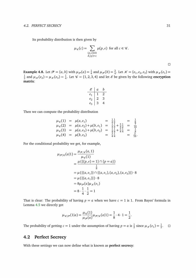
Its probability distribution is then given by
µC (c) =∑(p,e)∈ΩEe(p)=c
µ(p, e) for all c ∈ C .
Example 4.8. Let P = a, b with µP (a) = 14 and µP (b) = 3
4 . LetK = e1, e2, e3 with µK (e1) =12 and µK (e2) = µK (e3) =
14 . Let C = 1, 2, 3, 4 and let E be given by the following encryption
matrix:
E a be1 1 2e2 2 3e3 3 4
Then we can compute the probability distribution
µC (1) = µ(a, e1) = 14
12 = 1
8µC (2) = µ(a, e2) +µ(b, e1) =
14
14 +
34
12 = 7
16µC (3) = µ(a, e3) +µ(b, e2) =
14
14 +
34
14 = 1
4µC (4) = µ(b, e3) = 3
414 = 3
16 .
For the conditional probability we get, for example,
µP |C (a|1) = µP ,C (a, 1)
µC (1)
=µ ((p, e) = 1 ∩ p = a)
18
= µ ((a, e1) ∩ (a, e1), (a, e2), (a, e3)) · 8= µ ((a, e1)) · 8= 8µP (a)µK (e1)
= 8 · 14· 1
2= 1
That is clear: The probability of having p = a when we have c = 1 is 1. From Bayes’ formula inLemma 4.5 we directly get
µC |P (1|a) = µC (1)µP (a)
µP |C (a|1) = 18· 4 · 1= 1
2.
The probability of getting c = 1 under the assumption of having p = a is 12 since µK (e1) =
12 .
4.2 Perfect Secrecy
With these settings we can now define what is known as perfect secrecy:
32 CHAPTER 4. INFORMATION THEORY
Definition 4.9 (Shannon). A cryptosystem Π is called perfectly secret for µP if P and C areindependent, that is
∀p ∈ P , c ∈ C : µP (p) = 0 or µC |P (c|p) = µC (c) (or, equivalently,)∀p ∈ P , c ∈ C : µC (c) = 0 or µP |C (p|c) = µP (p).
We call Π perfectly secret if Π is perfectly secret for any probability distribution µP .
Example 4.10. The cryptosystem from Example 4.8 is not perfectly secret, since it is not perfectlysecret for the given µP : For a ∈ P and 1 ∈ C we have µP (a) = 1
4 = 0 and µC |P (1|a) = 12 = 1
8 =µC (1).
Remark 4.11. Perfect secrecy of a cryptosystem Πmeans that the knowledge of a ciphertext c ∈ Cdoes not yield any information on the plaintext p ∈ P .
The next properties are essential for perfect secret cryptosystems as we see in Lemma 4.14 andTheorem 4.22.
Definition 4.12. Let Π be a cryptosystem. We call Π resp. E transitive / free / regular if for each(p, c) ∈ P ×C there is one / at most one / exactly one e ∈K such that Ee(p) = c.
Lemma 4.13. Let Π be a cryptosystem. For each p ∈ P let p : K → C be the map defined bye 7→ Ee(p). Then it holds:
1. E is transitive iff for all p ∈ P p is surjective (|K | ≥ |C |).2. E is free iff for all p ∈ P p is injective (|K | ≤ |C |).3. E is regular iff for all p ∈ P p is bijective (|K |= |C |).4. |P |= |C | iff Ee :P →C is bijective for one e ∈K .
5. If E is free then |K |= |C | iff for all p ∈ P p is bijective.
Proof. Statements (1) – (3) follow trivially from Definition 4.12. Statement (4) follows from theinjectivity of the maps Ee : P → C due to the definition of Π. Statement (5) follows from theinjectivity condition of statement (2),
Lemma 4.14. If a cryptosystem Π is perfectly secret then Π is transitive.
Proof. Assume the contrary, E is not transitive. Thus there exists p ∈ P such that p :K →C is notsurjective. So we can choose a c ∈ C \ p(K ). By construction µP |C (p|c) = 0. By Convention 4.7the map Ω→ C is surjective, so there exists (p′, e) ∈ Ω such that Ee(p′) = c. Now we choose µPsuch that µP (p),µP (p′)> 0. Since µK (e)> 0 it follows that µC (c)≥ µP (p′)µK (e)> 0. We haveµC (c)> 0 and µP |C (p|c) = 0 = µP (p), thus Π is not perfectly secret.
Now we can easily conclude:
Corollary 4.15. Let a cryptosystemΠ be perfectly secret and free. ThenΠ is regular and |K |= |C |.
4.2. PERFECT SECRECY 33
Proof. Lemma 4.14 together with Lemma 4.13.
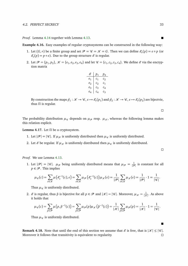
Example 4.16. Easy examples of regular cryptosystems can be constructed in the following way:
1. Let (G,) be a finite group and set P = C =K = G. Then we can define Ee(p) = e p (orEe(p) = p e). Due to the group structure E is regular.
2. Let P = p1, p2, K = e1, e2, e3, e4 and let C = c1, c2, c3, c4. We define E via the encryp-tion matrix
E p1 p2
e1 c1 c2e2 c2 c1e3 c3 c4e4 c4 c3
By construction the maps p1 :K →C , e 7→ Ee(p1) and p2 :K →C , e 7→ Ee(p2) are bijectvie,thus Π is regular.
The probability distribution µC depends on µP resp. µK , whereas the following lemma makesthis relation explicit.
Lemma 4.17. Let Π be a cryptosystem.
1. Let |P |= |C |. If µP is uniformly distributed then µC is uniformly distributed.
2. Let E be regular. If µK is uniformly distributed then µC is uniformly distributed.
Proof. We use Lemma 4.13.
1. Let |P | = |C |. µP being uniformly distributed means that µP = 1|P | is constant for all
p ∈ P . This implies
µC (c) =∑e∈KµE−1
e (c), e=∑e∈KµPE−1
e (c)µK (e) =
1|P |∑e∈KµK (e) =
1|P | · 1=
1|C | .
Thus µC is uniformly distributed.
2. E is regular, thus p is bijective for all p ∈ P and |K | = |C |. Moreover, µK = 1|K | . As above
it holds that
µC (c) =∑p∈Pµp, p−1(c)=∑p∈PµP (p)µKp−1(c)=
1|K |∑p∈PµP (p) =
1|K | · 1=
1|C | .
Thus µC is uniformly distributed.
Remark 4.18. Note that until the end of this section we assume that E is free, that is |K | ≤ |C |.Moreover it follows that transitivity is equivalent to regularity.
34 CHAPTER 4. INFORMATION THEORY
We state three further lemmata we need in order to prove Shannon’s theorem.
Lemma 4.19. Let Π be a cryptosystem, let E be regular and let µP be arbitrary. Π is perfectlysecret for µP iff
∀e ∈K , c ∈ C : µK ,C (e, c) = 0 or µK (e) = µC (c).
Proof. For perfect secrecy for µP we have to show that for all p ∈ P , c ∈ C it holds that µP (p) = 0or µC |P (c|p) = µC (c).⇒ Let µK ,C (e, c) > 0, then there exists p ∈ P such that Ee(p) = c and µP (p) > 0. Then p is
unique since Ee is injective. Since E is free, e is uniquely determined by p and c. Due to theindependence of P and K we follow:
µP (p)µK (e) = µP ,K (p, e) = µP ,C (p, c) = µC |P (c|p)µP (p) = µC (c)µP (p). (4.1)
Since µP (p)> 0 we conclude that µK (e) = µC (c).
⇐ Let c ∈ C and p ∈ P such that µP (p) > 0. E being regular implies that there exists exactlyone e ∈ K such that Ee(p) = c. By convention µK (e) > 0 thus µK ,C (e, c) > 0. Thus byassumption we have µC (c) = µK (e). Using Equation 4.1 again, we get µC (c) = µC |P (c|p).
Lemma 4.20. Let Π be a cryptosystem and let E be regular. Then Π is perfectly secret if µK isuniformly distributed.
Proof. By Lemma 4.17 µC is uniformly distributed. Since |K | = |C | holds we get µK (e) = 1|K | =
1|C | = µC (c). Now apply Lemma 4.19.
Lemma 4.21. Let Π be a cryptosystem, let E be regular and let µP be arbitrary. If Π is perfectlysecret for µP and if µC is uniformly distributed then µK is uniformly distributed.
Proof. Let e ∈K . Choose p ∈ P with µP (p)> 0. We set c := Ee(p) and get µK ,C (e, c)> 0. ThusµK (e) = µC (c) by Lemma 4.19.
Now we can state Shannon’s theorem.
Theorem 4.22 (Shannon). Let Π be regular and |P |= |C |. The following statements are equiva-lent:
1. Π is perfectly secret for µP (uniform distribution).
2. Π is perfectly secret.
3. µK is uniformly distributed.
Proof.
4.3. ENTROPY 35
(1)⇒ (3) By Lemma 4.17 µC is uniformly distributed. SinceΠ is regular it follows by Lemma 4.21that µK is uniformly distributed.
(3)⇒ (2) Follows by Lemma 4.20.
(2)⇒ (1) Trivial.
A well-known perfectly secret cryptosystem is the Vernam One-Time-Pad that was invented byFrank Miller in 1882 and patented by Gilbert S. Vernam in 1919.
Example 4.23 (Vernam One-Time-Pad). Let n ∈ N>0. We set P = C = K = (Z/2Z)n. Thekeys from K are chosen randomly and uniformly distributed. For each e ∈ K we define Ee(p) :=p ⊕ e ∈ C and De(c) := c ⊕ e ∈ P . By construction this cryptosystem is perfectly secret due toTheorem 4.22.
Clearly, there is a problem in applying Vernam’s One-Time-Pad in practice. Still there might bescenarios, for example, ambassadors or intelligence agencies, were one-time-pads are used.
Note that the condition of randomly choosing the keys is the other practical bottleneck as we willsee later on.
4.3 Entropy
In information theory the term entropy defines the expected value or average of the informationin each message of a transmission. In more detail, the amount of information of every event formsa random variable (see Section 4.1) whose expected value is the entropy. There are different unitsof entropy, here we use a bit (which is due to Shannon’s definition of entropy). Thus we assumebit representations of information.
For us, the entropy will be the key property in order to get rid of the assumption |P | = |C | inShannon’s theorem ( 4.22).
Definition 4.24. Let X : Ω→ M be a random variable for some finite set M . The entropy of X isdefined by
H(X ) := −∑x∈M
µX (x) lgµX (x)
where lg is shorthand notation for log2.2
Convention 4.25. In the following we will often abuse notation for X . So X denotes the underlyingset or language M = X as well as the corresponding random variable X .
Remark 4.26.
1. Since lima→0 a lg a = 0 we define 0 lg 0= 0.
2. From the properties of the logarithm we get also the alternative formulation
H(X ) =∑x∈M
µX (x) lg1
µX (x).
2What we call entropy is also known as binary entropy.
36 CHAPTER 4. INFORMATION THEORY
Lemma 4.27. Let X : Ω→ M be a random variable for some finite set M . It holds that H(X ) ≥ 0.In particular, H(X ) = 0 iff µX (x) = 1 for some x ∈ M .
Proof. Since µX (x) ∈ [0, 1] −µX (x) lgµX (x) ≥ 0 for all x ∈ M . Moreover, −µX (x) lgµX (x) = 0 iffµX (x) = 0 (see Remark 4.26) or µX (x) = 1.
Example 4.28.
1. Let’s assume we throw a coin with the events 0 and 1. Let µX (0) =34 and let µX (1) =
14 .
Then
H(X ) =34
lg43+
14
lg4≈ 0.81.
If we choose µX (0) = µX (1) =12 we get
H(X ) =12
lg2+12
lg2= 1.
2. Let |X |=: n<∞. If X is uniformly distributed then
H(X ) =n∑
i=1
1n
lg n= lg n.
Important for structuring messages into blocks of information are encodings.
Definition 4.29. Let X be a random variable and let f : X → 0, 1• be a map.
1. f is called an encoding of X if the extension to X •
f : X •→ 0, 1•, x1 · · · xn 7→ f (x1) · · · f (xn)
is an injective map for all n ∈ N>0.
2. f is called prefix-free if there do not exist two elements x , y ∈ X and an element z ∈ 0, 1•such that f (x) = f (y) z.
3. The average length of f is defined by
ℓ( f ) :=∑x∈M
µX (x)sz2 ( f (x)) .
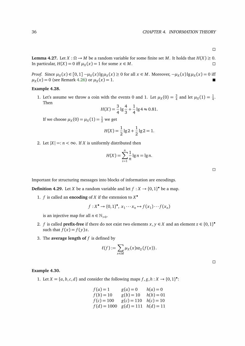
Example 4.30.
1. Let X = a, b, c, d and consider the following maps f , g, h : X → 0, 1•:f (a) = 1 g(a) = 0 h(a) = 0f (b) = 10 g(b) = 10 h(b) = 01f (c) = 100 g(c) = 110 h(c) = 10f (d) = 1000 g(d) = 111 h(d) = 11
4.3. ENTROPY 37
a) f is an encoding: Start at the end and read the encoding backwards. Once a 1 is reachedthe signal ends.
b) g is an encoding: One can start at the beginning and reads the encoding forwards. Everytime a known substring is found, this part is cut off: Let 10101110 be an encoding viag. We can read it as 10 10 111 0 thus we see: g(bbda) = 10 10 111 0. Moreover, g isa prefix-free encoding.
c) h is not an encoding since it is not injective on the extension to X •: h(ac) = 010= h(ba).
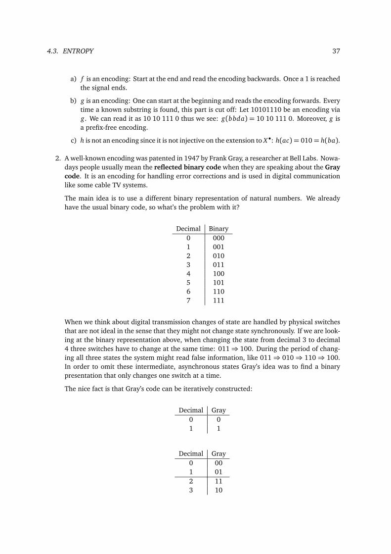
2. A well-known encoding was patented in 1947 by Frank Gray, a researcher at Bell Labs. Nowa-days people usually mean the reflected binary code when they are speaking about the Graycode. It is an encoding for handling error corrections and is used in digital communicationlike some cable TV systems.
The main idea is to use a different binary representation of natural numbers. We alreadyhave the usual binary code, so what’s the problem with it?
Decimal Binary0 0001 0012 0103 0114 1005 1016 1107 111
When we think about digital transmission changes of state are handled by physical switchesthat are not ideal in the sense that they might not change state synchronously. If we are look-ing at the binary representation above, when changing the state from decimal 3 to decimal4 three switches have to change at the same time: 011⇒ 100. During the period of chang-ing all three states the system might read false information, like 011⇒ 010⇒ 110⇒ 100.In order to omit these intermediate, asynchronous states Gray’s idea was to find a binarypresentation that only changes one switch at a time.
The nice fact is that Gray’s code can be iteratively constructed:
Decimal Gray0 01 1
Decimal Gray0 001 012 113 10
38 CHAPTER 4. INFORMATION THEORY
Decimal Binary0 0001 0012 0113 0104 1105 1116 1017 100
We can see that in Gray’s code going from one state to the next we only change exactly oneswitch. Moreover, the code is even reflected on the center line presented in the above tables:Generating a 3-digit Gray code, we use the 2-digit Gray code. We reflect the 2-digit code onthe centered line. Now for the upper half we add 0 as first digit, for the lower half we add 1as first digit.
Moreover, this Gray code is even cyclic: Cyclic means that once we reach the end (7 resp.100) we can start back with the beginning (0 resp. 000) and again change only one switch.
The idea is now that the entropy of X should be ℓ( f ) if f is the most efficient encoding for X .Here “most efficient” means that an event with probability 0< a < 1 is encoded by f (a) such thatsz2 (( f (a))) = − lg a = lg 1
a .
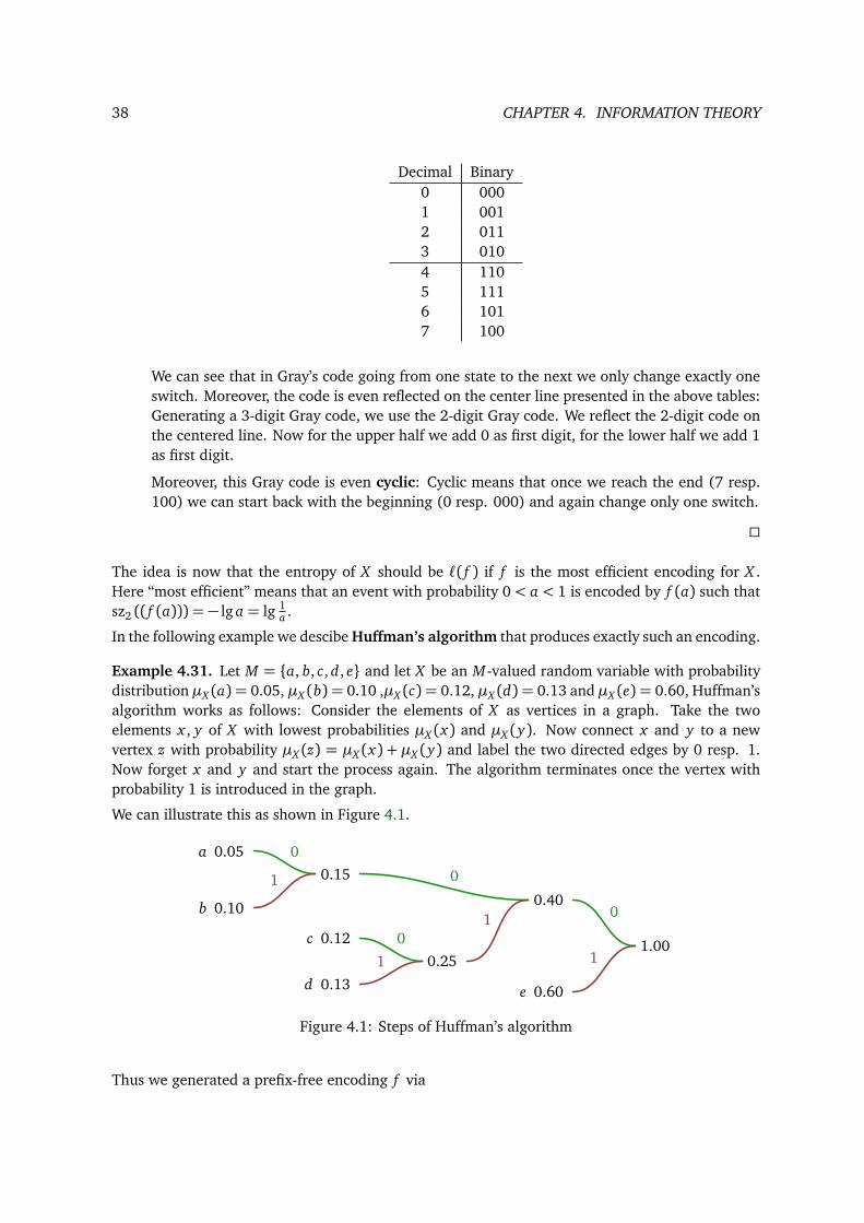
In the following example we descibe Huffman’s algorithm that produces exactly such an encoding.
Example 4.31. Let M = a, b, c, d, e and let X be an M -valued random variable with probabilitydistribution µX (a) = 0.05, µX (b) = 0.10 ,µX (c) = 0.12, µX (d) = 0.13 and µX (e) = 0.60, Huffman’salgorithm works as follows: Consider the elements of X as vertices in a graph. Take the twoelements x , y of X with lowest probabilities µX (x) and µX (y). Now connect x and y to a newvertex z with probability µX (z) = µX (x) + µX (y) and label the two directed edges by 0 resp. 1.Now forget x and y and start the process again. The algorithm terminates once the vertex withprobability 1 is introduced in the graph.
We can illustrate this as shown in Figure 4.1.
a 0.05
b 0.10
0.15
c 0.12
d 0.13
0.25
0.40
e 0.60
1.00
0
1
0
1
0
1 0
1
Figure 4.1: Steps of Huffman’s algorithm
Thus we generated a prefix-free encoding f via
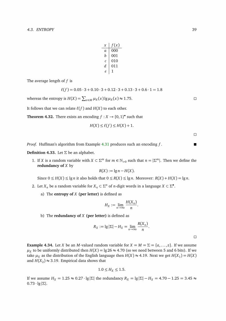
4.3. ENTROPY 39
x f (x)a 000b 001c 010d 011e 1
The average length of f is
ℓ( f ) = 0.05 · 3+ 0.10 · 3+ 0.12 · 3+ 0.13 · 3+ 0.6 · 1= 1.8
whereas the entropy is H(X ) =∑
x∈M µX (x) lgµX (x)≈ 1.75.
It follows that we can relate ℓ( f ) and H(X ) to each other.
Theorem 4.32. There exists an encoding f : X → 0, 1• such that
H(X )≤ ℓ( f )≤ H(X ) + 1.
Proof. Huffman’s algorithm from Example 4.31 produces such an encoding f .
Definition 4.33. Let Σ be an alphabet.
1. If X is a random variable with X ⊂ Σm for m ∈ N>0 such that n = |Σm|. Then we define theredundancy of X by
R(X ) := lg n−H(X ).
Since 0≤ H(X )≤ lg n it also holds that 0≤ R(X )≤ lg n. Moreover: R(X ) +H(X ) = lg n.
2. Let Xn be a random variable for Xn ⊂ Σn of n-digit words in a language X ⊂ Σ•.a) The entropy of X (per letter) is defined as
HX := limn→∞
H(Xn)n
.
b) The redundancy of X (per letter) is defined as
RX := lg |Σ| −HX = limn→∞
R(Xn)n
.
Example 4.34. Let X be an M -valued random variable for X = M = Σ = a, . . . , z. If we assumeµX to be uniformly distributed then H(X ) = lg26≈ 4.70 (so we need between 5 and 6 bits). If wetake µX as the distribution of the English language then H(X )≈ 4.19. Next we get H(X1) = H(X )and H(X2)≈ 3.19. Empirical data shows that
1.0≤ HX ≤ 1.5.
If we assume HX = 1.25 ≈ 0.27 · lg |Σ| the redundancy RX = lg |Σ| − HX = 4.70− 1.25 = 3.45 ≈0.73 · lg |Σ|.
40 CHAPTER 4. INFORMATION THEORY
What does this mean? Assume that tn is the number of equally probable texts in English languagefor text beginning of n letters. By HX = limn→∞ lg tn
n ≈ 1.25 we get tn ≈ 21.25·n for large n. Forexample, taking n = 20 we get t20 ≈ 3.35 · 107 whereas |Σ20| = 2620 ≈ 1.99 · 1028. So if we wantto attack some cryptosystem based on the English language and its probability distribution, a bruteforce attack can be optimized quite a lot, for example, by narrowing the plaintext space of 20 letterwords.
Remark 4.35. Note that a single text does not have an entropy. Only languages have an entropy.
We need some more ingredients in order to apply our knowledge of entropy and redundancy tocryptosystems.
Definition 4.36. Let X : Ω→ X and Y : Ω→ Y be two random variables with |X |, |Y |<∞.
1. The joint entropy of X and Y is defined by
H(X , Y ) := − ∑x∈X ,y∈Y
µX ,Y (x , y) lgµX ,Y (x , y).
2. The conditional entropy or equivocation of X and Y is defined by
H(X |Y ) :=∑y∈Y
µY (y)H(X |y)
whereH(X |y) := −∑
x∈X
µX |Y (x |y) lgµX |Y (x |y).
3. The transinformation of X and Y is defined by
I(X , Y ) := H(X )−H(X |Y ).
Theorem 4.37. Let X : Ω→ X and Y : Ω→ Y be two random variables with |X |, |Y |<∞.
1. H(X )≤ lg |X |. Equality holds iff µX is uniformly distributed.
2. H(X |Y )≤ H(X ). Equality holds iff X and Y are independent.
3. H(X |Y ) = H(X , Y )−H(Y ).
4. H(X , Y )≤ H(X ) +H(Y ). Equality holds iff X and Y are independent.
5. H(X |Y ) = H(Y |X ) +H(X )−H(Y ).
6. I(X , Y ) = I(Y, X )≥ 0.
Proof.
1. Exercise.
4.3. ENTROPY 41
2. This is a bit harder to prove, see, for example, Theorem 1.17 in [Mos17].
3. Exercise.
4. Exercise, where the equality statement follows from (2) and (3).
5. Follows from (3) taking into account that H(X , Y ) = H(Y, X ).
6. The equality follows from (5), the non-negativeness follows from (2).
Remark 4.38. Let X be a random variable and denote by X n the random variable describing then-fold independent repetition of the event X . Then H(X n) := H(X , . . . , X ) = nH(X ).
Convention 4.39. Until the end of this chapter we assume thatΠ is a symmetric cryptosystem suchthat P ,C ,K are finite (|C | ≥ |P | since Ee is injective), for all e ∈ K Ee is a map, and P and Kare independent.
Definition 4.40. In the above setting we define
1. the key equivocation H(K |C ) resp. the plaintext equivocation H(P |C ), and
2. the key transinformation I(K ,C ) resp. the plaintext transinformation I(P ,C ).
Lemma 4.41. Let Π be a cryptosystem as in Convention 4.39.
1. H(P ,K ) = H(K ,C ) = H(P ,C ,K ).2. H(C )≥ H(C |K ) = H(P |K ) = H(P ).3. H(K |C ) = H(P ) +H(K )−H(C ).4. I(K ,C ) = H(C )−H(P )≥ 0.
Proof.
1. H(P ,C ,K ) = H(C ,P ,K ) = H(C , (P ,K )) = H(C |(P ,K ))+H(P ,K ). By our assump-tions H(C |(P ,K )) = 0 as C is defined by P and K : Since Ee is injective for all e ∈ K wehave c = Ee(p) and thus p = De(c). It follows that H(P ,C ,K ) = H(P ,K ) = H(K ,C ).
2. H(C )≥ H(C |K ) is clear. For the equation we use (1):
H(C |K ) = H(C ,K )−H(K ) = H(P ,K )−H(K ) = H(P ) +H(K )−H(K ) = H(P ).3. Again we use (1):
H(K |C ) = H(K ,C )−H(C ) = H(P ,K )−H(C ) = H(P ) +H(K )−H(C ).4. We use (3):
I(K ,C ) = H(K )−H(K |C ) = H(K )−H(P )−H(K ) +H(C ) = H(C )−H(P ).Now by (2) it follows that H(C )−H(P )≥ 0.
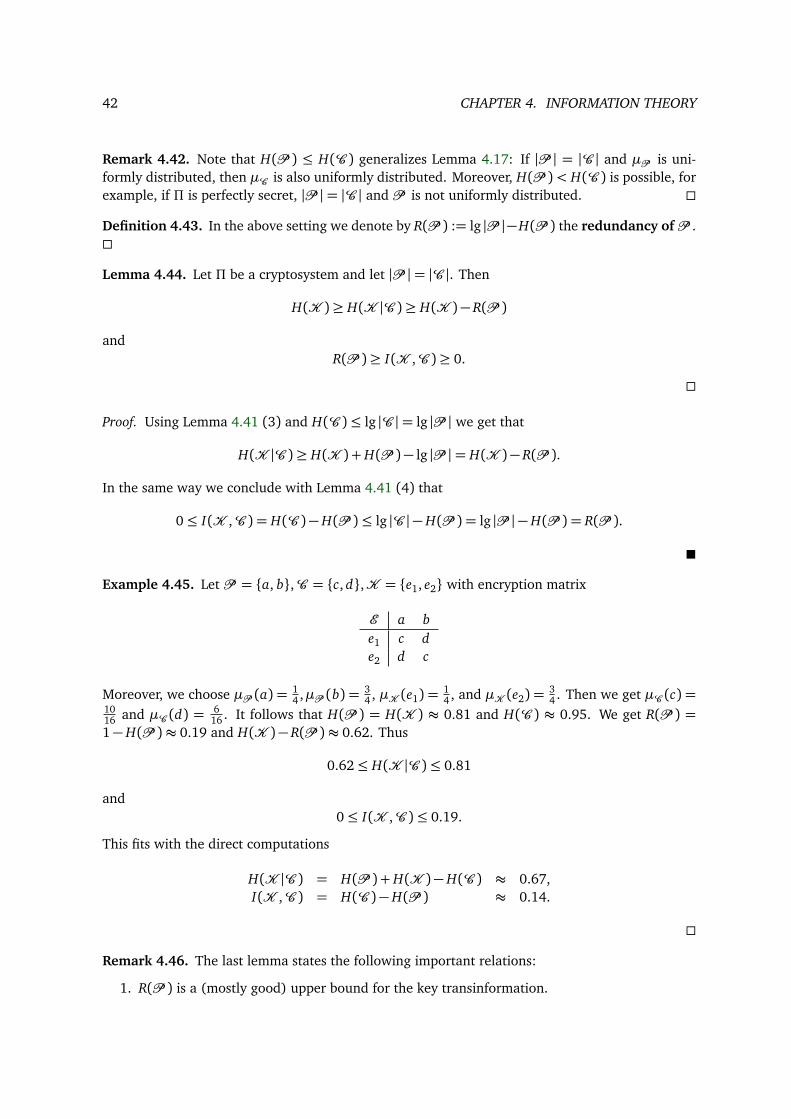
42 CHAPTER 4. INFORMATION THEORY
Remark 4.42. Note that H(P ) ≤ H(C ) generalizes Lemma 4.17: If |P | = |C | and µP is uni-formly distributed, then µC is also uniformly distributed. Moreover, H(P )< H(C ) is possible, forexample, if Π is perfectly secret, |P |= |C | and P is not uniformly distributed.
Definition 4.43. In the above setting we denote by R(P ) := lg |P |−H(P ) the redundancy of P .
Lemma 4.44. Let Π be a cryptosystem and let |P |= |C |. Then
H(K )≥ H(K |C )≥ H(K )− R(P )and
R(P )≥ I(K ,C )≥ 0.
Proof. Using Lemma 4.41 (3) and H(C )≤ lg |C |= lg |P | we get that
H(K |C )≥ H(K ) +H(P )− lg |P |= H(K )− R(P ).In the same way we conclude with Lemma 4.41 (4) that
0≤ I(K ,C ) = H(C )−H(P )≤ lg |C | −H(P ) = lg |P | −H(P ) = R(P ).
Example 4.45. Let P = a, b,C = c, d,K = e1, e2 with encryption matrix
E a be1 c de2 d c
Moreover, we choose µP (a) = 14 ,µP (b) = 3
4 , µK (e1) =14 , and µK (e2) =
34 . Then we get µC (c) =
1016 and µC (d) = 6
16 . It follows that H(P ) = H(K ) ≈ 0.81 and H(C ) ≈ 0.95. We get R(P ) =1−H(P )≈ 0.19 and H(K )− R(P )≈ 0.62. Thus
0.62≤ H(K |C )≤ 0.81
and0≤ I(K ,C )≤ 0.19.
This fits with the direct computations
H(K |C ) = H(P ) +H(K )−H(C ) ≈ 0.67,I(K ,C ) = H(C )−H(P ) ≈ 0.14.
Remark 4.46. The last lemma states the following important relations:
1. R(P ) is a (mostly good) upper bound for the key transinformation.
4.3. ENTROPY 43
2. We need at least as much key entropy H(K ) as we have redundancy in P in order to get anonnegative lower bound for the key equivocation H(K |C )≥ H(K )− R(P ).
3. If P is uniformly distributed then R(P ) = 0 thus also I(K ,C ) = 0 and H(K ) = H(K |C ).
Example 4.47. Let K = C = Σk and let L ⊂ Σ• be a language with entropy HL and redundancyRL .3 Let P ⊂ L. For n big enough we get
H(K |C )≥ H(K )− R(P )≈ H(K )− nRL .
In other words: If H(K ) is fixed and n can grow, for example via repeated encryption with thesame key, then the entropy is exhausted as n increases.
This leads to the following definition:
Definition 4.48. With notation as in Example 4.47 the number n0 :=
H(K )RL
£is called the unicity
distance.
Remark 4.49. The higher the redundancy of a language the faster a key is exhausted. So oneneeds to compensate the redundancy of a language, for example, by increasing the key size.
Let us look on values for n0 in practical examples:
Example 4.50. Let |Σ|= 26 and L be the English language with RL = 3.45.
symmetric cryptosystem |K | H(K ) n0
monoalphabetic substitution 26!≈ 288.4 ≈ 88.4 26
permutation of 16-blocks 16!≈ 244.3 ≈ 44.3 13
“DES” (see Section 6.2) 256 56 17
“AES” (see Section 6.3) 2128 128 38
Let us assume a text length of n= 20 and the monoalphabetic substitution. Then we get
H(K |C )≥ H(K )− R(P ) = H(K )− 20RL ≈ 88.40− 20 · 3.45= 19.40.
Thus we have approximately 219.4 ≈ 691 802 keys to try. This is done in seconds on a usual personalcomputer.
So what we want to do is to increase the unicity distance but still keep the key lengths short inorder to have a fast and efficient cryptosystem. There are several attempts to do this:
Remark 4.51.
1. Reduce the redundancy of P , for example, by compressing (zipping) the text.
3Note that one can define the entropy of a language with non fixed word length in more generality, also we do notdo this here.
44 CHAPTER 4. INFORMATION THEORY
2. Cover the redundancy of P against attackers with limited computing power, for example, byusing combinations of substitution and so-called Feistel ciphers (see Section 6.1)
3. Try to bloat the key entropy against attackers with limited computing power by using so-called autokey ciphers: These ciphers include the plaintext in the key itself, for example,when using Vigenère’s cipher with autokey we would have something like this:
plaintext dies erte xtxxkey keyd iese rtex
4. Use pseudo random sequences for the key. Still, getting pseudo random elements is not trivialat all.
We finish this chapter with further investigations on free cryptosystems.
Lemma 4.52. Let Π be a cryptosystem.
1. H(P ,K ) = H(P ,C ) +H(K |(P ,C )).2. H(K ) = H(C |P ) +H(K |P ,C ).3. H(K |C ) = H(P |C ) +H(K |P ,C ).4. Π free⇔ H(K |(P ,C )) = 0⇔ I(K , (P ,C )) = H(K ).
Proof.
1. H(K |(P ,C )) = H(K ,P ,C )−H(P ,C ) = H(K ,P )−H(P ,C ).2. By assumption P and K are independent, thus H(P |K ) = H(P ).
H(P |K ) = H(P ,K )−H(K ) (1)= H(P ,C ) +H(K |(P ,C ))−H(K )= H(C |P ) +H(P ) +H(K |(P ,C ))−H(K ).
It follows:H(K ) = H(C |P ) +H(P )−H(P |K ) +H(K |(P ,C )).
By assumption H(P )−H(P |K ) = 0 thus the statement follows.
3. Using (1) we get
H(K |C ) = H(K ,C )−H(C ) = H(P ,K )−H(C )= H(P ,C ) +H(K |(P ,C ))−H(C ) = H(P |C ) +H(K |(P ,C )).
4. I(K , (P ,C )) = H(K )− H(K |(P ,C )). If Π is free then the map p : K → C , e 7→ Ee(p)is injective for all p ∈ P . So µK |(P ,C )(e|(p, c)) is 0 if the combination is not possible and 1if Ee(p) = c and thus H(K |P ,C ) = 0. If H(K |(P ,C )) = 0 then each e ∈ K is uniquelydefined by p and c, thus the map p is injective for all p ∈ P . So Π is free.
4.3. ENTROPY 45
Remark 4.53. We can interpret H(K |(P ,C )) as the unused key entropy and I(K |(P ,C )) asthe used key entropy.
Theorem 4.54. Let Π be a free cryptosystem.
1. H(P |C ) = H(K |C ) = H(P ) +H(K )−H(C ).2. I(P ,C ) = H(C )−H(K ).3. H(K )≤ H(C ).
Proof. By Lemma 4.52 (3) we have H(P |C ) = H(K |C )− H(K |P ,C ). Since Π is free it followsfrom 4.52 (4) that H(K |P ,C ) = 0. By Lemma 4.41 (3)we know that H(K |C ) = H(P )+H(K )−H(C ) which proves statement (1). For statements (2) and (3) we see that
0≤ I(P ,C ) by def.= H(P )−H(P |C ) (1)= H(P )−H(K |C ) (1)= H(C )−H(K ).
Corollary 4.55. Let Π be a free cryptosystem.
1. If |P |= |C | then H(P |C )≥ H(K )− R(P ).2. If |K |= |C | then I(P ,C )≤ R(K ).
Proof.
1. By Theorem 4.54 (1) H(P |C ) = H(K |C ). The statement is then just Lemma 4.44.
2. By Theorem 4.54 (2) we have I(P ,C ) = H(C )−H(K ), thus
I(P ,C ) = H(C )−H(K )≤ lg |C | −H(K ) = lg |K | −H(K ) = R(K ).
As already explained at the beginning of this section our goal is to generalize Shannon’s theorem(4.22) by removing the assumption that |P |= |C |.Theorem 4.56. Let Π be a cryptosystem as in Convention 4.39. Then the following statements areequivalent:
1. Π is perfectly secret for µP (i.e. P and C are independent).
2. I(P ,C ) = 0.
3. H(P ,C ) = H(P ) +H(C ).4. H(C |P ) = H(C ).5. H(P |C ) = H(P ).
46 CHAPTER 4. INFORMATION THEORY
If we further assume that Π is free, and thus in our setting regular, the list of equivalences alsoincludes:
6. H(K ) = H(C ).7. H(K |C ) = H(P ) which implies H(K )≥ H(P ).
Proof. The equivalence of (1)− (5) is trivial. By Lemma 4.52 (2) and (4) we know that H(K ) =H(C |P ). So (6) follows by (4) and vice versa. By Lemma 4.52 (3) and (4)we have that H(K |C ) =H(P |C ). Thus (7) follows by (5) and vice versa.
Corollary 4.57 (Shannon). Let Π be a free cryptosystem. Then Π is perfectly secret for µP andµC is uniformly distributed iff |K |= |C | and µK is uniformly distributed.
Proof.
⇒ Since µC is uniformly distributed we know that H(C ) = lg |C |. Π is free, so |K | ≤ |C |.Since we assume perfect secrecy for µP and Π is free we get H(K ) = H(C ) = lg |C | byTheorem 4.56 (6). By definition µK is then uniformly distributed and thus also |K |= |C |.
⇐ By Theorem 4.54(3) H(K )≤ H(C ). Since µK is uniformly distributed we have the inequality
lg |K |= H(K )≤ H(C )≤ lg |C |. (4.2)
Since |K |= |C | equality must hold in 4.2. HenceµC is uniformly distributed, H(K ) = H(C )and Π is perfectly secret for µP by Theorem 4.56 (1)⇔ (6).
Chapter 5
Pseudorandom Sequences
In the last chapters we have often spoken about randomness and pseudorandomness. Most of ourassumptions on perfect secrecy and big enough unicity distances depend on random or pseudoran-dom input data. Next we try to give these notions some mathematical meaning.
5.1 Introduction
Possible sources of random sequences (RS) might be
• white noise captured by your laptops microphone,
• throwing a perfect coin, or
• quantum mechanical systems producing statistical randomness.
Pseudorandomness on the other hand starts with a short random source produced in a way likeexplained above. A pseudorandom sequence is then generated in a deterministic way, i.e. by analgorithm, having this random seed as input. Pseudorandom sequences (PRS) have advantages anddisadvantages:
Advantages
1. PRS can be produced by software instead of hardware.
2. PRS can be reconstructed: Assume its usage in a cryptosystem. One just has to exchangethe random seed and the algorithm generating the PRS.
Disadvantages
1. The seed must be random, otherwise the PRS can be easily recovered.
2. Moreover, the seed must be secret, otherwise the complete PRS is known.
3. Clearly, the algorithm producing the PRS is deterministic and can thus be attacked.
Possible applications of PRS are the generation of session keys (web session, messenger, etc.),stream ciphers (see Section 3.3) or the generation of TANs and PINs (online banking, etc.).
Example 5.1. One example we have already seen are linear feedback shift registers, see Defini-tion 3.20.
47
48 CHAPTER 5. PSEUDORANDOM SEQUENCES
5.2 Linear recurrence equations and pseudorandom bit generators
Convention 5.2. In the following, let K be a field, let ℓ ∈ N and let c = (c0, . . . , cℓ−1)tr ∈ Kℓ withc0 = 0.
Definition 5.3. A linear recurrence equation LRE for c of degree ℓ > 0 is given by
sn+ℓ =sn · · · sn+ℓ−1 · c0
...cℓ−1
(n≥ 0) (5.1)
such that
1. t(0) := t =t0 · · · tℓ−1 ∈ K1×ℓ is the initial value,
2. si = t i for 0≤ i ≤ ℓ− 1, and
3. t(n) :=sn · · · sn+ℓ−1
is the n-th state vector.
Since the full information of the sequence s lies in c and t we also write s := ⟨c, t⟩.
Example 5.4. Taking K = F2, ℓ= 4, c =
1100
and t =1 0 1 0
we get:
s = 1, 0, 1, 0, 1, 1, 1, 1, 0, 0, 0, 1, 0, 0, 1, | 1, 0, 1, 0, . . .
Remark 5.5. A linear recurrence equation over K = F2 (abbreviated by F2-LRE) of degree ℓ isnothing but an ℓ-bit Linear Feedback Shift Register (LFSR) [Wik17e]. It is an example of a linearpseudorandom bit generator (PRBG) (cf. Example 5.65). It is one among many pseudorandombit generators [Wik17g].
Definition 5.6.
1. Define χ := χc := xℓ − cℓ−1 xℓ−1 − · · · − c1 x − c0 ∈ K[x].
2. s is called k-periodic (k ∈ N) if si+k = si for all i ≥ 0, or equivalently, t(i+k) = t(i) for all i ≥ 0.
3. c is called k-periodic (k ∈ N) if s = ⟨c, t⟩ is k-periodic for all t ∈ K1×ℓ.
4. If s (resp. c) is k-periodic for some k ∈ N then denote by per(s) (resp. per(c)) the smallestsuch number and call it the period length. If such a k does not exist then set per s :=∞(resp. per c :=∞).
Lemma 5.7. With s, c and t defined as in Definition 5.3 the following statements hold:
1. sn+ℓ = t(n) · c.
5.2. LINEAR RECURRENCE EQUATIONS AND PSEUDORANDOM BIT GENERATORS 49
2. t(n) = t(n−1) · C = t · Cn with
C :=
0 · · · · · · 0 c01 0 · · · 0 c1
0... . . .
......
.... . . . . . 0 cℓ−2
0 · · · 0 1 cℓ−1
.
3. ⟨c, t⟩ is k-periodic if and only if t · Ck = t.
4. c is k-periodic if and only if Ck = Iℓ.
5. per⟨c, t⟩=mink > 0 | t · Ck = t.6. per c =mink > 0 | Ck = Iℓ.7. ⟨c, t⟩ is k-periodic iff per⟨c, t⟩ | k.
8. per c = lcmper⟨c, t⟩ | t ∈ K1×ℓ.9. per⟨c, 0⟩= 1.
10. C is the companion matrix1 of χ. Hence, χ is the minimal polynomial and therefore also thecharacteristic polynomial of C (as its degree is ℓ).
11. C is a regular matrix since c0 = 0, i.e., C ∈ GLℓ(K).
12. per c = ord C in GLℓ(K).
13. The cyclic subgroup ⟨C⟩ generated by the matrix C acts on the vector space K1×ℓ. The orbit2
t · ⟨C⟩= t(i) | i ∈ Z of t is nothing but the set of all reachable state vectors.
14. per⟨c, t⟩= |t · ⟨C⟩|.
Proof. (1) – (13) are trivial. To see (14) note that the state vectors t(i) with 0 ≤ i < per⟨c, t⟩ arepairwise distinct: t(i) = t( j) for 0 ≤ i ≤ j < per⟨c, t⟩ means that tC i = tC j and hence tC j−i = twith j − i < per⟨c, t⟩. Finally this implies that j = i.
Linear algebra
Let K be a field, V a nontrivial finite dimensional K vector space, φ ∈ EndK(V ), and 0 = v ∈ V .
Recall, the minimal polynomial mφ is the unique monic3 generator of the principal ideal Iφ := f ∈ K[x] | f (φ) = 0 ∈ EndK(V ), the so-called vanishing ideal of φ.
Analogously, the minimal polynomial mφ,v with respect to v is the unique monic generator ofthe principal ideal Iφ,v := f ∈ K[x] | f (φ)(v) = 0 ∈ V, the so-called vanishing ideal of φ withrespect to v.
1German: Begleitmatrix2German: Bahn3German: normiert
50 CHAPTER 5. PSEUDORANDOM SEQUENCES
Exercise 5.8. For 0 = v ∈ V let Uφ,v := ⟨φi(v) | i ∈ N0⟩ ≤ V . Then
1. mφ,v = mφ|Uφ,v.
2. dimK Uφ,v =mind ∈ N | (v,φ(v), . . . ,φd(v)) are K–linearly dependent ≥ 1.
3. deg mφ,v = dimK Uφ,v .
4. mφ = lcmmφ,v | 0 = v ∈ V. This gives an algorithm to compute the minimal polynomial ofφ as the lcm of at most ℓ minimal polynomials mφ,v1
, . . . , mφ,vℓ , where ℓ= dimK V .
5. α ∈ EndK(V ) is an automorphism if and only if mα(0) = 0 ∈ K . This gives an algorithm tocompute the inverse of α.
Definition 5.9. Let 0 = f ∈ K[x] and let k ∈ N. We define the order of f : If f (0) = 0 we define
ord f :=mink > 0 : f | xk − 1 or∞.
If f (0) = 0, then we write f = x r f with r ∈ N minimal such that f (0) = 0 and we define
ord f := ord f .
Definition 5.10. Let α ∈ AutK(V ) and ⟨α⟩ the cyclic subgroup of AutK(V ) generated by α. By
ordα := |⟨α⟩|denote the order of the group element α. For v ∈ V denote the orbit of v under the action of thecyclic subgroup ⟨α⟩ as usual by
⟨α⟩v := αi(v) | i ∈ Z.
Proposition 5.11. Let α ∈ AutK(V ).
1. ord mα = ordα.
2. ord mα,v = |⟨α⟩v| for v = 0.
3. If mα is irreducible then |⟨α⟩v|= ord mα for all v = 0.
4. If K is finite and mα irreducible then ord mα | (|V | − 1).
5. If there exists a vector v ∈ V with ⟨α⟩v = V \ 0 then mα is irreducible.
Proof.
1. Follows from the equivalence
αk = idV ⇐⇒ (xk − 1)(α) = 0 ⇐⇒ mα | xk − 1.
5.2. LINEAR RECURRENCE EQUATIONS AND PSEUDORANDOM BIT GENERATORS 51
2. If |⟨α⟩v| <∞ then there exists 0 ≤ i < j with αi(v) = α j(v). Hence, α j−i(v) = v. Therefore(even if |⟨α⟩v|=∞)
|⟨α⟩v| = mink > 0 | αk(v) = v= mink > 0 | (αk − idV )(v) = 0 ∈ V= mink > 0 : mα,v|xk − 1= ord mα,v .
3. If mα is irreducible then the statements mα,v | mα and deg mα,v > 0 are equivalent to mα,v =mα. (2) completes the argument.
4. Follows from (3) which implies that the orbits of ⟨α⟩ in V \ 0 are all of the same length:For all v, w ∈ V \ 0 |⟨α⟩v| = |⟨α⟩w|. It follows that |V | = |K |ℓ for some ℓ ∈ N. Moreover,|V |= 1+ k · ord mα
4, i.e. ord mα | |V | − 1.
5. First note that if ⟨α⟩v = V \0 for one v ∈ V then also for all v ∈ V \0 (being all elementsof the orbit). In particular, assume that Uα,v ⊊ V . Then there exists w ∈ V \ Uα,v , i.e. thereexists i < 0 such that αi(v) = w due to our initial note. Thus we can write v = α−i(w) and getUα,v ⊊ Uα,w. All in all, we can assume that there exists v ∈ V such that Uα,v = V and hencemα,v = mα for all v = 0. If mα = gh we want to prove that either mα | g or mα | h: For v = 0we obtain 0 = mα,v(α)(v) = (gh)(α)(v) = (g(α) h(α))(v) = g(α)(h(α)(v)). Hence, eitherh(α)(v) = 0 or v′ := h(α)(v) = 0 and g(α)(v′) = 0. In other words, either mα = mα,v | h ormα = mα,v′ | g.
Period length
Convention 5.12. Let V = K1×ℓ and t ∈ V \0. Identify AutK(V ) with GLℓ(K) in the obvious way.Viewing the regular matrix C (of Lemma 5.7.(2)) as an automorphism we get χ = mC . Defineχt := mC ,t .
Corollary 5.13. With c and ℓ defined as above the following statements hold:
1. per c = ordχ.
2. per⟨c, t⟩= ordχt for t = 0.
3. If χ is irreducible then per⟨c, t⟩= per c for all t = 0.
And in case K = Fq (i.e., finite with q elements):
4. If χ is irreducible then per c | qℓ − 1.
5. If per c = qℓ − 1 then χ is irreducible.
Proof. All statements follow easily from Lemma 5.7 and Proposition 5.11.
Moreover, we can follow that there always exists a t such that the period length of c is reached.
4The +1 comes from 0 ∈ V .
52 CHAPTER 5. PSEUDORANDOM SEQUENCES
Corollary 5.14. Again, let c, t and ℓ defined as above. Then there exists a (row) vector t ∈ K1×ℓwith per⟨c, t⟩= per c.
Proof. We denote by C the companion matrix. Let ei = (0, . . . , 0, 1, 0, . . . , 0) denote the ith basisvector of K1×ℓ. We compute the orbit of eℓ w.r.t. C:
eℓ · C0 = eℓeℓ · C1 = eℓ−1 + cℓ−1eℓ
(eℓ · C) · C = eℓ · C2 = eℓ−2 + cℓ−1eℓ−1 +c2ℓ−1 + cℓ−2
eℓ
...
By the above construction it is clear that the orbit of eℓ w.r.t. C has length |eℓ⟨C⟩| ≥ ℓ. Now, due tothe linear independency of the ei and using notation from Exercise 5.8 we see that UC ,ℓ = V = K1×ℓdue to dimension reasons. Thus by Exercise 5.8 (1) we get
mC ,ℓ = mC|UC ,ℓ= mC .
We conclude with Corollary 5.13 (1) & (2):
per c = ordχ = ord mC = ord mC ,ℓ = ordχℓ = per⟨c,ℓ⟩.
Example 5.15. Let K = F2.
1. Consider the 3-bit LFSR (i.e., of degree ℓ= 3) and maximum possible period length qℓ−1=23 − 1= 8− 1= 7.
ctr χ irred. s orbit lengths
(1, 0, 0) x3 + 1 false 100|100, 110|110, 1|111 3+ 3+ 1
(1, 1, 0) x3 + x + 1 true 1001011|100 7
(1, 0, 1) x3 + x2 + 1 true 1001110|100 7
(1, 1, 1) x3 + x2 + x + 1 false 1001|100, 01|010, 1|111 4+ 2+ 1
Note that, for example,
(x2 + x + 1)(x + 1) = x3 + x2 + x + x2 + x + 1= x3 + 2x2 + 2x + 1= x3 + 1 over F2.
2. Consider the 4-bit LFSR (i.e., of degree ℓ= 4) and maximum possible period length qℓ−1=24 − 1= 16− 1= 15.
ctr χ irred. s orbit lengths
(1, 1, 0, 0) x4 + x + 1 true 100010011010111|1000 15
(1, 0, 0, 1) x4 + x3 + 1 true 100011110101100|1000 15
(1, 1, 1, 1) x4 + x3 + x2 + x + 1 true 10001|1000, 01001|0100 5+ 5+ 5
10100|1010...
......
......
5.3. FINITE FIELDS 53
Definition 5.16. We call a linear recurrence equation irreducible if χ is irreducible. If moreoverK = Fq is a finite field then we call the LRE transitive if per c = qℓ − 1, where ℓ is its degree.
Remark 5.17. There are faster ways to compute per c and to decide the transitivity of LREs. Con-sider for example c = (1, 1, 0, 0)tr with χ = x4 + x + 1 in the above table. Since χ is irreduciblewe know from Corollary 5.13 that ordχ | 15. It is obvious that χ ∤ xk − 1 for k = 1, 3, 5 (theseare the divisors of 15). Hence per c = ordχ = 15, the maximal possible period length, i.e., thecorresponding LFSR is transitive.
Exercise 5.18. Classify all irreducible 4-bit LFSR. How many of them are transitive?
Remark 5.19. The Mersenne twister [Wik17f] is a modern pseudorandom bit generator with animpressive period length of per c = 219937 − 1 ≈ 4.3 · 106001. Its name comes from the fact that219937 − 1 is a Mersenne prime number.
5.3 Finite fields
For a better understanding on how to get good pseudorandom bit generators let us recall someideas from finite field theory.
Convention 5.20. In the following all fields are finite fields if not otherwise stated.
Field extensions
Recall, if K ≤ L is a field extension, then L is a K-vector space. The degree of the field extensionK ≤ L is defined as the dimension of L as a K-vector space:
[L : K] := dimK L.
For a 2-step field extension K ≤ L ≤ M the degree formula
[M : K] = [M : L] · [L : K]
is a direct consequence of the definition.
In what follows we only deal with finite field extensions K ≤ L, i.e., where
d := [L : K]<∞.
For any element α ∈ L the d + 1 elements 1,α, . . . ,αd are always K–linearly dependent, whichleads us to the next definition:
Definition 5.21. Let K ≤ L be a finite field extension and let α ∈ L. The unique monic generator ofthe vanishing (principal) ideal Iα,K := f ∈ K[x] | f (α) = 0 is called the minimal polynomialof α over the ground field K , and denoted by mα,K , or simply mα, if no confusion can occur aboutthe ground field K .
Remark 5.22. In the above definition the field L can be replaced by a (finite dimensional) K-algebra L. This gives a common generalization of the two definitions mφ and mα,K above, wherein the former case L = EndK(V ).
54 CHAPTER 5. PSEUDORANDOM SEQUENCES
Remark 5.23. Let K ≤ L be a finite field extension of degree d and α ∈ L. The minimal polynomialmα = mα,K satisfies the following properties:
1. For f ∈ K[x] it holds: f (α) = 0 ⇐⇒ mα | f .
2. mα is irreducible in K[x] and 1≤ deg mα ≤ d.
3. If an irreducible monic polynomial f ∈ K[x] satisfies f (α) = 0 then f = mα.
We now recall Kronecker’s construction of field extensions:
Exercise 5.24. Let K be a field and f ∈ K[x]. The residue class K-algebra L := K[x]/⟨ f ⟩ is afield if and only if f is irreducible. In this case [L : K] = deg f and m x = m x ,K = f , wherex := x + ⟨ f ⟩ ∈ K[x]/⟨ f ⟩.
Example 5.25.
1. Let f := x − a for a ∈ K . Then K[x]/⟨ f ⟩ ∼= K .
2. Let K be a subfield of R, e.g., K = Q or K = R. Then f = x2 + 1 is irreducible and the fieldK[x]/⟨ f ⟩ is an extension of degree 2 over K with (1, x) as a K-basis satisfying x2 = −1.
3. Let K = F2 and f = x3+ x +1. The degree 3 polynomial f is irreducible since it has no rootsin its field of definition F2. The field L := F2[x]/⟨ f ⟩ is an extension of degree 3 over F2 with(1, x , x2) as an F2-basis and elements
L = 0, 1, x , x2, 1+ x , x + x2, 1+ x + x2, 1+ x2.
Order of field elements
Lemma 5.26. Let K be a field.
1. Let f ∈ K[x] be irreducible and f = x . Then x = 0 in L := K[x]/⟨ f ⟩ and ord f = ord x inthe multiplicative group L∗ := (L \ 0, ·).
2. Let K ≤ L be a (finite) field extension and α ∈ L∗. Then ord mα,K = ordα in the multiplicativegroup L∗.
Proof.
1. xk = 1 ⇐⇒ f | xk − 1.
2. αk = 1 ⇐⇒ α is a root of xk − 1 ⇐⇒ mα,K | xk − 1.
Corollary 5.27. Let K = Fq be a finite field with q elements and f ∈ Fq[x] of degree n. Then
1. f irreducible =⇒ ord f | qn − 1.
5.3. FINITE FIELDS 55
2. ord f = qn − 1 =⇒ f irreducible.
Proof. We can assume that f is monic.
First assume that f (0) = 0: Take V = K1×n and β ∈ AutK(V )with mβ = f (e.g., β : t 7→ t ·C , whereC is the companion matrix of f , which is due to f (0) = 0 regular). Now apply Proposition 5.11(4) and (5) for both statements.
Now we assume that f (0) = 0:
1. f = x is the only irreducible monic polynomial with f (0) = 0. By definition ord x5.9:= ord1=
1.
2. Now let f = x r f for some r ≥ 1, i.e. f is not irreducible. By construction deg f = n− r andf (0) = 0. By Definition 5.9 we know that ord f = ord f . If f is irreducible we know by (1)that ord f | qn−r−1. Otherwise we consider the product f =
∏fi and do the same argument
for the irreducible factors fi . Glueing this information back together (a bit technical) we getan estimate for ord f < qn − 1. All in all, it follows that ord f < qn − 1.
Definition 5.28. Let K = Fq be a finite field with q elements and L a finite field extension of Fq.
1. A degree n polynomial f ∈ Fq[x] is called primitive if ord f = qn−1. Primitive polynomialsare irreducible by the above corollary.
2. An element α ∈ L∗ is called primitive5 if ordα= |L∗|, i.e., if L∗ = ⟨α⟩ := αi | i ∈ N0.
Lemma 5.29. Let K = Fq a finite field with q elements.
1. Let f ∈ Fq[x] be a primitive polynomial and L := Fq[x]/⟨ f ⟩. Then x is a primitive elementof L.
2. If Fq ≤ L is a finite field extension then α ∈ L∗ is primitive iff mα,K is a primitive polynomial(of degree [L : K]).
Proof.
1. Define n := deg f . Then |L|= qn and |L∗|= qn−1. Now use that ord x5.26.(1)= ord f = qn−1.
2. Define n := [L : K]. If L∗ = ⟨α⟩ then ordα = |L∗| = qn − 1. Set f = mα,K . Lemma 5.26.(2)implies that ord f = ordα = qn − 1. Using that deg f ≤ n and that ord f | qdeg f − 1 (Corol-lary 5.27.(1)) we conclude that n= deg f and finally the primitivity of f = mα,K .
Exercise 5.30. Let L := F2[x]/⟨ f ⟩ and
1. f := x3 + x + 1. Prove that f is a primitive polynomial, or equivalently, that x ∈ L is aprimitive element, i.e., L∗ = ⟨ x⟩.
5Unfortunately, this name conflicts the notion of primitive elements of (algebraic) field extensions.
56 CHAPTER 5. PSEUDORANDOM SEQUENCES
2. f := x4 + x3 + x2 + x + 1. First prove that L is a field. Prove that f is an imprimitivepolynomial, or equivalently, that x ∈ L is an imprimitive6 element, i.e., L∗ = ⟨ x⟩
Some field theory
Let K be a field. Recall:
1. K[x] is a Gaussian domain7. A more suggestive name is unique factorization domain(UFD) or simply factorial domain8.
2. For f ∈ K[x] the following holds:
a) f (a) = 0 ⇐⇒ (x − a) | f .
b) f (a) = f ′(a) = 0 ⇐⇒ (x − a)2 | f , where f ′ is the derivative of f w.r.t. x .
3. The characteristic of K is defined as char K =minc ∈ N | c ·1= 0 or 0. i.e., it is the uniquenonnegative generator of the principal ideal ker(Z→ K , c 7→ c · 1) Ã Z. char K is either zeroor a prime number.
4. If char K = p > 0 then Fp ≤ K . Else Q ≤ K . The fields Fp∼= Z/pZ resp. Q = Quot(Z)
are therefore called prime fields. Each field contains exactly one prime field as the smallestsubfield.
5. For a finite field extension K ≤ L define for an element α ∈ L the smallest subring of Lcontaining K and α
K[α] :=
¨ n∑i=1
λiαi | n ∈ N0,λi ∈ K
«.
6. The vanishing ideal Iα,K = ⟨mα,K⟩ is the kernel of the ring epimorphism K[x]→ K[α], x 7→ α.Hence K[α] ∼= K[x]/⟨mα,K⟩ as K-algebras and K(α) := K[α] is a field with [K(α) : K] =deg mα,K . The field K(α) is called the intermediate field9 generated by α.
Example 5.31. Let L := F2[x]/⟨x4 + x3 + x2 + x + 1⟩ as in Exercise 5.30.(2). The element α :=x3+ x2+1 satisfies α2 = x3+ x2. Hence mF2,α = x2+ x +1 and F2(α) = F2[α] is an intermediatefield of degree [F2(α) : F2] = 2: K(α) = K + Kα= 0, 1,α, 1+α.
Proposition 5.32. Let K ≤ L be a field extension and let f ∈ K[x] be a monic irreducible polyno-mial with f (α) = f (α′) = 0 for two elements α,α′ ∈ L. Then K(α) ∼= K(α′) as K-algebras (or asfields over K).
Proof. f (α) = 0 and f monic irreducible implies f = mα,K by Remark 5.23.(3). The same ist truefor α′. Hence K(α)∼= K[x]/⟨ f ⟩ ∼= K(α′).
Now we recall the notion of the splitting field of a polynomial f ∈ K[x].
6Although x is a primitive element of the field extension F2 ≤ F2[ x] = F2[x]/⟨x4 + x3 + x2 + x + 1⟩.7German: Gaußcher Bereich8German: Faktorieller Bereich9German: Zwischenkörper
5.3. FINITE FIELDS 57
Definition 5.33. Let K ≤ L and f ∈ K[x]. We define the following properties:
1. f splits over10 L if f splits as a product of linear factors (when viewed as a polynomial) overL[x].
2. L is a splitting field11 of f over K if f splits over L and L is minimal with this property.
Remark 5.34. If f splits over L with roots α1, . . . ,αn then K(α1, . . . ,αn) = K[α1, . . . ,αn] is asplitting field of f contained in L.
Theorem 5.35. For each f ∈ K[x] there exists a splitting field, unique up to K-isomorphism.
Proof. The above remark shows that it is enough to construct a field M ≥ K over which f splits.We may assume12 that f is irreducible (otherwise we do the following for all factors). The fieldL := K[x]/⟨ f ⟩ contains (at least) one root of f which is α := x . Hence f = (x − α) f ∈ L[x].Proceed by induction on deg f resp. deg f .
It follows that we can talk about the splitting field of f over K . Recall, char K = p > 0 means thatpα= 0 for any α in any field extension L ≥ K .
Lemma 5.36. Let K be a field with char K = p > 0. For each i ∈ N0 the map φi : K → K , x 7→ x piis
an automorphism of K which fixes the prime field Fp. It is called the i-th Frobenius automorphismof K .
Proof. Since φi = φi1 it suffices to consider i = 1. Of course 1p = 1 and (αβ)p = αpβ p in any field
of any characteristic. We therefore only need to prove the “characteristic p formula”
(α± β)p = αp ± β p.
Indeed the binomial theorem (α+β)p =∑p
k=0
pk
αkβ p−k implies the statement since
p0
=p
p
= 1
and p | pk for 0< k < p. Proving the bijectiveness is an exercise.
Theorem 5.37. Let K be a field of prime characteristic p, n ∈ N, and q := pn. Consider f :=xq − x ∈ Fp[x].
1. f splits over K if and only if K contains exactly one subfield with q elements.
2. K is the splitting field of f if and only if |K |= q.
Proof. SetN := α ∈ K | f (α) = 0.
10German: zerfällt über11German: Zerfällungskörper12It is not clear how to make this step constructive. From the constructive point of view, we have just assumed that
we have an algorithm to factor polynomials in irreducible factors.
58 CHAPTER 5. PSEUDORANDOM SEQUENCES
1. By construction |N | ≤ q. Since f has no multiple roots ( f ′ = −1 =⇒ gcd( f , f ′) = 1) weconclude that f splits over K ⇐⇒ |N |= q. The previous lemma implies that N is a subfieldof K: α,β ∈ N =⇒ (α−β)q = αq−βq = α−β and we are done with the forward implicationin (1).Now let M ≤ K be a subfield with q elements. Since |M∗|= q−1 it follows that every α ∈ M∗is a root of f = x(xq−1 − 1), hence M ≤ N . From |N | ≤ q we conclude that M = N . Thisproves the uniqueness of M = N and that f splits over a field K containing N . This provesstatement (1).
2. (2) follows from (1) and the minimality of the splitting field.
Corollary 5.38.
1. If K is a finite field then char K = p > 0 and |K |= pn for a prime p.
2. For each prime power q = pn there exists up to Fp-isomorphism exactly one field with qelements.
Proof.
1. Since K is finite its characteristic char K = p > 0 is prime. Hence, Fp is the prime field of Kand, in particular, K is an Fp-vector space. So |K |= pn, where n= [K : Fp] := dimFp
K .
2. Follows from Theorem 5.37.(2) and the uniqueness of the splitting field applied to the poly-nomial f = xq − x .
We have been referring to this field as Fq. Now we can say “the field Fq”.
Corollary 5.39. The finite field Fq = Fpn contains the unique subfield (isomorphic to) Fpd if andonly if d | n. I.e.
Fpd ≤ Fpn ⇐⇒ d | n.
In other word, the subfield lattice13 of Fpn is isomorphic to the lattice of divisors of n (regardlessof the prime number p).
Proof. Let K ≤ Fq = Fpn . Then K has characteristic p and the prime field Fp of Fq is the prime fieldof K . Hence K = Fpd for some 1≤ d ≤ n. The degree formula n= [Fpn : Fp] = [Fpn : Fpd ] [Fpd : Fp]︸ ︷︷ ︸
dimplies that d | n.Now we prove the converse. Let d | n. First note that αpd
= α implies αpn= α. In particular, the
roots of x pd − x are also roots of x pn − x . So x pd − x splits over Fpn . Theorem 5.37.(1) then statesthat Fpn contains the unique field with pd elements.
Example 5.40.
13German: Zwischenkörperverband
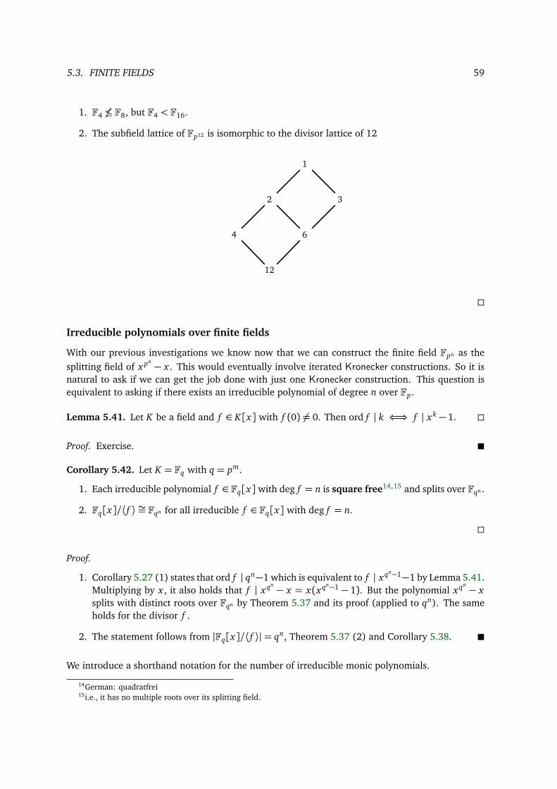
5.3. FINITE FIELDS 59
1. F4 ≤ F8, but F4 < F16.
2. The subfield lattice of Fp12 is isomorphic to the divisor lattice of 12
1
2
4
3
6
12
Irreducible polynomials over finite fields
With our previous investigations we know now that we can construct the finite field Fpn as thesplitting field of x pn − x . This would eventually involve iterated Kronecker constructions. So it isnatural to ask if we can get the job done with just one Kronecker construction. This question isequivalent to asking if there exists an irreducible polynomial of degree n over Fp.
Lemma 5.41. Let K be a field and f ∈ K[x] with f (0) = 0. Then ord f | k ⇐⇒ f | xk − 1.
Proof. Exercise.
Corollary 5.42. Let K = Fq with q = pm.
1. Each irreducible polynomial f ∈ Fq[x] with deg f = n is square free14,15 and splits over Fqn .
2. Fq[x]/⟨ f ⟩ ∼= Fqn for all irreducible f ∈ Fq[x] with deg f = n.
Proof.
1. Corollary 5.27 (1) states that ord f | qn−1 which is equivalent to f | xqn−1−1 by Lemma 5.41.Multiplying by x , it also holds that f | xqn − x = x(xqn−1 − 1). But the polynomial xqn − xsplits with distinct roots over Fqn by Theorem 5.37 and its proof (applied to qn). The sameholds for the divisor f .
2. The statement follows from |Fq[x]/⟨ f ⟩|= qn, Theorem 5.37 (2) and Corollary 5.38.
We introduce a shorthand notation for the number of irreducible monic polynomials.
14German: quadratfrei15i.e., it has no multiple roots over its splitting field.
60 CHAPTER 5. PSEUDORANDOM SEQUENCES
Notation 5.43. Set
A(d) = A(d, q) := | f ∈ Fq[x] : f irreducible monic with deg f = d|.
For the following theorem we need a small preparation:
Lemma 5.44. Letπ be the the product of all monic irreducible polynomials f over Fq with deg f | n.Then π= xqn − x .
Proof. By Corollaries 5.39 and 5.42 we know that each monic irreducible polynomial f with deg f |n fulfills f | xqn − x . Since we are working over a principal ideal domain and, thus, all these f arealso prime we know that π | xqn − x . Now, using again Corollary 5.39 we get π= xqn − x .
Theorem 5.45. For K = Fq the numbers A(d) satisfy∑d|n
dA(d) = qn. (5.2)
In particular, A(1) = q and A(d) = qd−qd if d is prime.
Proof. Set L := Fqn . We know that Fqd ≤ L ⇐⇒ d | n. First note that by Lemma 5.44 xqn − x isthe product of all monic irreducible polynomials f ∈ Fq[x] with deg f | n. By counting the degreeswe directly get the formula
∑d|n dA(d) = qn as each such polynomial of degree d contributes d to
the total degree.If d is prime, note that there exists no intermediate subfield between Fqd and Fq as the field ex-
tension has prime degree d. Thus every monic irreducible polynomial dividing xqd − x has eitherdegree d or degree 1. There exist exactly q linear such polynomials. Again summing up all suchpolynomials we have A(d) monic irreducible polynomials of degree d, we can again count thedegree:
dA(d) + q = qd .
This finishes the proof.
Example 5.46. Let q = 2. Now we list all minimal polynomials (= irreducible monic polynomials)together with their degrees for the following fields:
1. K = F22
mα,F2x x + 1 x2 + x + 1
deg 1 1 2∑= 4
2. K = F24
mα,F2 x x + 1 x2 + x + 1 x4 + x + 1 x4 + x3 + 1 x4 + x3 + x2 + x + 1
deg 1 1 2 4 4 4∑= 16
5.3. FINITE FIELDS 61
Remark 5.47. We list the following facts without proof:
1. Asymptotically: A(d)∼ qd
d .
2. Since Equation 5.2 is an inclusion-exclusion counting formula over a lattice one can use theMöbius function
µ(d) :=
1 , d = 10 , d is not square free
(−1)k , d is the product of k distinct primes
to “invert” it:
A(n) = A(n, q) =1n
∑d|nµ(d)q
nd .
Example 5.48. A(20, q) = 120(q
20 − q10 − q4 + q2).
Primitive polynomials
Counting primitive polynomials is much simpler.
Proposition 5.49. Let K be a field and U a finite subgroup of K∗. Then U is cyclic.
Proof. Exercise.
Corollary 5.50. Let φ denote Euler’s totient function:16. Let q = pd .
1. There are exactly φ(q− 1) primitive elements in F∗q.
2. There are exactly φ(q−1)d primitive monic polynomials of degree d in Fp[x].
Proof.
1. Proposition 5.49 implies that the multiplicative group F∗q = a0, a1, . . . , aq−2 is cyclic. In
particular, ai is primitiveDef 5.28⇐⇒ F∗q = (ai)k | k ∈ N0 ⇐⇒ gcd(i, q− 1) = 1.
2. Every primitive f ∈ Fp[x] of degree d is the minimal polynomial of exactly d primitiveelements in L = Fpd = Fq. This follows from the irreducibility of f (Corollary 5.27.(2)) andLemma 5.29 using (1) and the same argument as in the proof of Theorem 5.45.
Example 5.51. In the following two examples we mainly sum up computations we did before:
16German: Recall: φ(n) = |(Z/nZ)∗| = |i|0≤ i ≤ n s.t. gcd(i, n) = 1| = n∏
p|n1− 1
p
for distinct primes p divid-
ing n. φ is multiplicative, φ(mn) = φ(m)φ(n) if gcd(m, n) = 1. For p prime and k ≥ 1 we have φ(pk) = pk − pk−1 =pk1− 1
p
.
62 CHAPTER 5. PSEUDORANDOM SEQUENCES
1. For p = 2 and d = 2 we get q = 22 = 4. F4 = F22 = 0, 1,ω, 1+ω with ω2 +ω+ 1 = 0. ωand 1+ω are all primitive elements of F4 and their minimal polynomial x2+ x + 1 the onlyirreducible and primitive polynomial of degree 2 over F2.
2. Let q = 16, so we could have p = 2 and d = 4 or p = 4 and d = 2. There are φ(16− 1) = 8primitive elements in F16 = F24 = F42 . Hence there are 8
2 = 4 primitive polynomials
x2 + x +ω, x2 + x +ω2, x2 +ωx +ω, x2 +ω2 x +ω2
of degree 2 over F4 and 84 = 2 primitive polynomials
x4 + x + 1, x4 + x3 + 1
of degree 4 over F2. The polynomial x4 + x3 + x2 + x + 1 = x5−1x−1 is the only irreducible
imprimitive polynomial of degree 4 over F2.
Example 5.52. We compare A(d) and the number of primitive polynomials of degree d over F2:
d 1 2 3 4 5 6 7 8 9 10 11 16
A(d, 2) 2 1 2 3 6 9 18 30 56 99 186 4080
primitive 2 1 2 2 6 6 18 16 48 60 176 2048
We will be using primitive polynomials χ over finite fields to construct pseudorandom sequencess = ⟨c, t⟩ of maximal possible period lengths (cf. Definition 5.6). Since χ = χc will be part of thesecret key, we need to know how to randomly choose primitive polynomials. The idea will be torandomly choose a polynomial and then to test its primitiveness.
5.4 Statistical tests
Let Xn and Un denote random variables with values in 0, 1n where Un is the uniformly distributedone. Note that any map f : 0, 1n→ 0, 1m induces a random variable Ym := f Xn.
Example 5.53. Define linear pseudorandom bit generator G as the map
G :
0, 12ℓ → 0, 1•(c, t) 7→ ⟨c, t⟩ ,
where we consider the pair (c, t) as an ℓ-bit LFSR given by c ∈ Fℓ×12 and initial value t ∈ F1×ℓ
2 . Bytruncation to the first n bits we get a map
Gn :
0, 12ℓ → 0, 1n(c, t) 7→ ⟨c, t⟩i=0,...,n−1
Define the random variableX := G U2ℓ
5.4. STATISTICAL TESTS 63
In other words, X is a (linear) pseudorandom bit generator with random seed. Define the finiterandom variable
Xn := Gn U2ℓ
with values in 0, 1n.
Our goal will be to compare Xn with Un.
Definition 5.54. A (polynomial) statistical test is a polynomial probabilistic algorithm
A :
0, 1• → 0, 1s 7→ A(s) .
We say that s ∈ 0, 1• passes the test A if A(s) = 1.
Remark 5.55. The composition A Xn is a random variable with values in 0, 1 for any randomvariable Xn (with values in 0, 1n). µAXn
(1) is the probability that an s ∈ 0, 1n that was chosenaccording to Xn passes the test A.
The idea is to construct statistical tests A where s ∈ 0, 1n only passes A if it was chosen randomly,i.e., according to Un.
Statistical randomness
The idea is to choose a statisticS : 0, 1•→ R
such that the distribution of SUn converges to a continuous probability density f . A continuous17
real valued random variable X : Ω → R has a probability density f : R → R≥0 satisfying theprobability PX (I) = P(X ∈ I) =
∫I f (x)d x for any interval I ⊂ R .
Example 5.56. Forα ∈ (0, 1) choose an interval I ⊂ R (as small as possible) with∫
I f (x)d x > 1−α,or, equivalently,
∫R\I f (x)d x < α. Define the statistical test A := AS,α induced by the statistic S
by setting
AS,α(s) :=
1 if S(s) ∈ I0 if S(s) ∈ I
.
Then µAUn(1)> 1−α and, equivalently, µAUn
(0)< α. The real number α is called the significancelevel18.
Recall that the expected value of the real valued random variable X with density f can be computedas E(X ) :=∫
x∈R x f (x)d x . The variance19 is defined by
Var(X ) := E((X − E(X ))2) = E(X 2)− E(X )2.
Remark 5.57. Let X , Y be two (finite) random variables and a, b, c ∈ R.
17German: stetig (hat zwei Bedeutungen!)18German: Signifikanzniveau19German: Varianz
64 CHAPTER 5. PSEUDORANDOM SEQUENCES
1. E is linear, i.e.E(aX + bY ) = aE(X ) + bE(Y ).
2. If X and Y are independent then
Var(aX + bY + c) = a2 Var(X ) + b2 Var(Y ).
3. Assume that Y is discrete and uniformly distributed, and that (Y1, . . . , Yn) is the n-fold inde-
pendent repetition of the experiment Y . Then Zn :=∑n
i=1
Yi−E(Y )p
n Var(Y )
=∑n
i=1 Yi−nE(Y )pn Var(Y )
con-
verges to the standard normal distribution20 N(0, 1) with expected value 0 and variance 1(see Appendix A.1).
Proof. E(Zn) = 0 due to the linearity of E.Var(Zn) =
1n Var(Y ) Var∑n
i=1 Yi − nE(Y )= 1
n Var(Y ) Var∑n
i=1 Yi
= n Var(Y )
n Var(Y ) = 1.
Example 5.58. We now give two examples of polynomial statistical tests.
1. Monobit (or balance) test: Since E(U1) =12 and Var(U1) =
14 we define the statistic S :
0, 1•→ RS(s0s1 · · · sn−1) :=
∑i si − n
2Æ n4
=2∑
i si − npn
.
according to Remark 5.57.(3). Hence S Un is an approximation of N(0, 1) for n large.For a given significance level α ∈ (0, 1) choose I = (−x , x) with erfc( xp
2) < α, i.e., x <p
2erfc−1(α). Define
A :
0, 1n → 0, 1
s 7→
1 if |S(s)|< x0 otherwise
=
1 if |∑i si − n
2 |< d0 otherwise
,
where d :=Æ
n2 erfc−1(α). Then µAUn
(1) > 1 − α and, equivalently, µAUn(0) < α. For
example, a bit sequence of length n = 20000 passes the monobit test with significance levelα= 10−6 if the number of ones lies in the interval ( n
2 − d, n2 + d)≈ (9654, 10346).
2. Autocorrelation test: The autocorrelation test on the bit sequence s = (si) ∈ FN02 with dis-
tance d is the monobit test on the bit sequence s′ = (si + si+d) ∈ FN02 .
3. There are many more such tests. See, for example, the so-called runs test [Wik16f].
Remark 5.59. LFSR have good statistical properties; in particular, their output passes all statisticaltests in the above example. Indeed, if A is the monobit test then µAXn
(1) ≈ 1 for Xn = Gn U2ℓ(cf. Example 5.53).
Sketch of Proof. Each period of a primitive ℓ-bit LFSR (with maximal possible period length 2ℓ−1)consists of exactly 2ℓ−1 − 1 zeros and 2ℓ−1 ones.
20German: Standard-Normalverteilung
5.4. STATISTICAL TESTS 65
Unpredictability
Passing all statistical randomness tests is not enough for a pseudorandom bit generator to be cryp-tographically secure. It must be “unpredictable” as well.
Remark 5.60 (Predictability of an LFSR ). Let s = ⟨c, t⟩ be the output of an ℓ-bit LFSR of which 2ℓconsecutive bits are known, say s0, . . . , s2ℓ−1, w.l.o.g. Hence the ℓ consecutive vectors t(0), . . . , t(ℓ−1) ∈F1×ℓ
2 are known. They satisfy the equation t(0)...
t(ℓ−1)
· c = sℓ
...s2ℓ−1
.This inhomogeneous linear system is solvable by our assumption on s. And there exists a uniquesolution for c if and only if t(0), . . . , t(ℓ−1) are F2-linearly independent. In this case the next-bits2ℓ = (sℓ · · · s2ℓ−1) · c can be predicted. This last condition is satisfied when the LFSR is irreducibleand t(0) = 0.
Example 5.61. For ℓ= 4 and s = 10101111?? . . . we solve1 0 1 00 1 0 11 0 1 10 1 1 1
· c =111
1
and obtain the unique solution c =
1100
. The complete sequence is 101011110001001|1010
(cf. Example 5.15): We get χc = x4 + x + 1 with period length ordχc = 24 − 1= 15.
Definition 5.62. Let P be a statistical test. The next-bit test with predictability P is the statisticaltest A := AP defined by
s = s0 · · · sn 7→ AP(s) =
0 if P(s0 · · · sn−1) = sn1 if P(s0 · · · sn−1) = sn
.
In other words, 0 for correct prediction and 1 for incorrect prediction. Note that if P is polynomialthen so is AP .
Example 5.63 (Linear predictability of an LFSR ). Define the statistical test P by setting
P(s) := (sℓ · · · s2ℓ−1) · cwhere s = s0 · · · s2ℓ−1 ∈ 0, 12ℓ and c computed as in Remark 5.60 (a not necessarily uniquesolution). Remark 5.60 implies21 that µAPX2ℓ+1
(1) = 0 for X2ℓ+1 = G2ℓ+1 U2ℓ (cf. Example 5.53).It follows that an LFSR is (linearly) predictable and in its original form cryptographically insecure.
21We skipped some details here. For example, since P is defined only for |s| even, AP is a priori only defined for|s| odd. To define it for |s| = 2r we set AP(s) := AP(s0 . . . s2r−2). The non-uniqueness of c has to be addressed as well(cf. [Wik16a].)
66 CHAPTER 5. PSEUDORANDOM SEQUENCES
5.5 Cryptographically secure pseudorandom bit generators
Again, let Xn and Un be random variables with values in 0, 1n where Un is the uniformly dis-tributed one.
Definition 5.64.
1. A polynomial deterministic algorithm G : 0, 1• → 0, 1• is called a pseudorandom bitgenerator (PRBG) if there is a function n : N→ N with n(k)> k and G(0, 1k) ⊂ 0, 1n(k)for all k ∈ N. The function n is called the stretch function of G.
2. A function f : N → R is called negligible22 if for each positive polynomial p there exists ak0 ∈ N such that | f (k)|< 1
p(k) for all k ≥ k0. The function f (k) = e−k is a prominent exampleof a negligible function.
3. We say that G passes the statistical test A if
k 7→ µAGUk(1)−µAUn(k)
(1)
is negligible.
4. G is called cryptographically secure (CSPRBG) if G passes all polynomial statistical tests.
In other words, G is cryptographically secure if an adversary with limited computational resourceshas no non-negligible advantage in predicting the next bit of the pseudorandom sequence.
Example 5.65. Let n : N→ N be an arbitrary function with n(k)> k for all k ∈ N. Define G by
Gn(k)(a0a1 · · · ak−1) := ⟨a0 · · · aℓ−1, aℓ · · · a2ℓ−1⟩i=0,...,n(k)−1, ℓ :=
k2
,
the PRBG corresponding to LFSR (cf. Example 5.53). For P as in Example 5.63 we obtainµAPGUk
(1) − µAPUn(k)(1) ≡ −1
2 , not negligible. Hence, LFSR are not cryptographically secure.
Note that this holds even for n : k 7→ k + 1: We have only 2k possible pseudorandom strings oflength k+ 1, in contrast to all 2 · 2k = 2k+1 possible random strings of length k+ 1.
We state without proof:
Theorem 5.66 (Yao). A PRBG is cryptographically secure iff it is unpredictable, i.e., iff it passesall polynomial next-bit tests.
Empirical security
The problem with the LFSR is basically their linearity. Here are some attempts to destroy thislinearity.
1. The first idea is to use the complete state vector t(n) = t(n−1)C instead of simply returningits last entry sn+ℓ. For this use a non-linear “filter function” f : F1×ℓ
2 → F2, which will beregarded as part of the secret key:
22German: vernachlässigbar
5.5. CRYPTOGRAPHICALLY SECURE PSEUDORANDOM BIT GENERATORS 67
Example 5.67. The following is known as Knapsack23 generator: Given a primitive ℓ-bitLFSR (i.e., with period 2ℓ−1), fix a natural number k > lgℓ and choose in some random waynon-negative integers a0, . . . , aℓ−1. Together with the initial vector they build the secret key.Define the filter function f (u) := (k-th last bit of
∑ui=1 ai) where u = (u0 . . . uℓ−1) ∈ F1×ℓ
2represents the current state vector.
2. The second idea is to combine several LFSR clocked24 in different ways:
Example 5.68 (Alternating step generator). Let R be an LFSR generating a sequence r =(rn), and let S and S′ be two different LFSR. Use R to reclock S and S′ by setting
sℓ+i := t(i) · c and s′ℓ+i := s′
ℓ+i−1, if ri = 0,s′ℓ+i := t ′(i) · c′ and sℓ+i := sℓ+i−1, if ri = 1.
Define the resulting sequence to be (si + s′i) (in the notation of Definition 5.3).
3. The third idea is that an LFSR throws away parts of another LFSR:
Example 5.69 (Shrinking generator). Two LFSR are running in parallel and produce the bitsequences s and s′. If s′i = 1 the bit si is returned, otherwise it is discarded25.
Provable security
Let f : 0, 1• → 0, 1• be a polynomial deterministic algorithm. The question of whether thereexists a polynomial algorithm that computes preimages of f leads us to the next fundamentaldefinition:
Definition 5.70. Let f : 0, 1•→ 0, 1• be a polynomial deterministic algorithm.
1. For an arbitrary polynomial probabilistic algorithm A : 0, 1•→ 0, 1• define
A f : 0, 1•→ 0, 1, x 7→
1 if A( f (x)) ∈ f −1 ( f (x))0 otherwise
.
f is called a one-way function (OWF)26 if k 7→ µA f Uk(1) is negligible for all A.
2. Let b : 0, 1•→ 0, 1 be a polynomial deterministic algorithm. For an arbitrary polynomialstatistical test (i.e., a polynomial probabilistic algorithm) A : 0, 1•→ 0, 1 define
A f ,b : 0, 1•→ 0, 1, x 7→
1 if A( f (x)) = b(x)0 otherwise
.
b is called a hardcore predicate27 (or hardcore bit, or hidden bit) of f if k 7→ µA f ,bUk(1)− 1
2is negligible for all A.
23German: Rucksack24German: getaktet25German: verworfen26German: Einwegfunktion27German: Hardcore-Prädikat, oder Sicherheitsbit
68 CHAPTER 5. PSEUDORANDOM SEQUENCES
This means that a OWF f is easy to compute (polynomial deterministic) but hard to invert. Ahardcore predicate b of a function f is a function that outputs a bit: If f is a OWF, then upon inputf (x) it is infeasible to correctly guess b(x) with a non-negligible knowledge/advantage above 1
2 .Clearly, one can always guess the bit b(x) with probability 1
2 . The hardcore predicate tries toexplain in a concentrated sense the hardness of inverting the function f .
Remark 5.71.
1. If f is injective (in other words, does not lose information) and has a hardcore predicate thenf is a OWF.
2. The existence of a hardcore predicate does not imply the injectivity of f . For example,the non-injective function f defined by f (s0s1 · · · sn) = s1 · · · sn has the hardcore predicateb(s0s1 · · · sn) = s0.
Definition 5.72. A one-way permutation (OWP ) is a bijective one-way function which is lengthpreserving, i.e., f (0, 1n) ⊂ 0, 1n and f : 0, 1n→ 0, 1n is a permutation for all n ∈ N>0.
Theorem 5.73. Let f be a OWP with hardcore predicate b and n : N → N an arbitrary functionwith n(k) > k which is bounded by some polynomial and which is computable by a polynomialrun-time algorithm. Then the function G : 0, 1•→ 0, 1• defined by
Gn(k)(s) := b(s)b( f (s)) · · · b( f n(k)−1(s))
is a CSPRBG with stretch function n.
Proof. ConsiderG′n(k)(s) := b( f n(k)−1(s)) · · · b( f (s))b(s).
Assume G′ is not cryptographically secure. Then Yao’s Theorem would imply the existence of anext-bit test AP which G′ does not pass. But this contradicts b being a hardcore bit of f . The proofis complete since cryptographic security does not depend on the order of the output.
Lemma 5.74. Let f be a OWP. Then
g : 0, 12n→ 0, 12n, (x , y) 7→ ( f (x), y)
with |x |= |y| defines a OWP with the Goldreich-Levin hardcore predicate b given by b(x , y) :=∑ni=1 x i yi ∈ F2.
Proof. This is a corollary of the Goldreich-Levin Theorem, see [Tre05].
Corollary 5.75. The existence of a CSPRBG is equivalent to the existence of a OWP.
Proof. The backward implication follows from Theorem 5.73 and Lemma 5.74. The forward im-plication is an exercise.
5.5. CRYPTOGRAPHICALLY SECURE PSEUDORANDOM BIT GENERATORS 69
Remark 5.76. There is also the concept of a pseudoramdom function family. It is a family of ef-ficiently computable functions that have the following property: No efficient algorithm can dis-tinguish with a significant advantage between a function chosen from the family and a so-calledrandom oracle. In practice often block ciphers are used where pseudorandom functions (for only alimited number of input and key sizes) are needed. In general, there is the concept by Goldreich–Goldwasser–Micaii to construct pseudorandom functions from pseudorandom generators.
A CSPRBG based cryptosystem
We finish this chapter by constructing a cryptosystem based on a (public) CSPRBG G with stretchfunction n.
Example 5.77. Define the symmetric cryptosystem (P ,C ,K ,E ,D) with P = C = 0, 1•, K =0, 1k for some security parameter k := ⌈lg |K |⌉ ∈ N (e.g., k = 128), and E as follows:For each p ∈ P choose randomly a key e ∈K and a seed s ∈K and compute G(s) ∈ 0, 1n(k). Set
c = Ee(p) := (s+ e) · (p+ G(s))0,...,|p|−1,
where + is the bitwise addition and · the concatenation of bits. So |c| is slightly bigger than |p|. If|p|> n(k) then choose several random seeds. This cryptosystem has at least two advantages:
1. After receiving s+ e one can compute s and start the computation of G(s).
2. The receiver can decrypt c bitwise.
Chapter 6
Modern Symmetric Block Ciphers
In Chapter 4 we have seen that in order to get perfectly secret cryptosystems Shannon’s theorystates what is to do: It boils down to the idea of Vernam’s one-time-pad, see Example 4.23. Clearly,in practice one could not apply these conditions. But we have seen in Remark 4.51 that there areseveral ideas to increase the unicity distance. Two main concepts that build the basis for modernsymmetric block ciphers are confusion and diffusion:
Definition 6.1. Let Π be a cryptosystem.
1. Confusion is the concept that a digit resp. bit of the ciphertext c ∈ C depends on severalparts of the key e ∈K .
2. Diffusion is the concept that if we change a digit resp. bit of the plaintext p ∈ P then theimpact on the ciphertext c ∈ C is unpredictable. Statistically speaking: Changing one bit ofp should change half of the bits of c. In the same way: If we change one bit of c then half ofthe bits of p should change.
These concepts are the underlying ideas of the well-known symmetric block ciphers DES and AESwe discuss in the following. As a building block we first have a look at the so-called Feistel cipher.
6.1 Feistel cipher
The following ideas go back to Horst Feistel who worked at IBM. The cipher was first seen com-mercially in IBM’s Lucifer cipher designed by Feistel and Don Coppersmith.
Let Σ= Z/2Z= F2 = 0, 1 be an alphabet. The Feistel cipher is a block cipher of block length 2nfor n ∈ N>0, so P = C = Σ2n. One fixes some key space K , a number of rounds r ∈ N>0 as wellas a method on how to construct from one key k ∈ K a tuple (k0, . . . , kr−1) of sub-keys for eachround. For each sub-key ki we denote by fki
: Σn → Σn the round function of the Feistel cipher.Let p ∈ P we subdivide p = (L0, R0) such that L0, R0 ∈ Σn. In each round 0≤ i < r one computes
(Li+1, Ri+1) = (Ri , Li ⊕ fki(Ri)).
The encryption function of the Feistel cipher is then given by
Ek(p) = Ek((L0, R0)) = (Rr , Lr) = c.
70
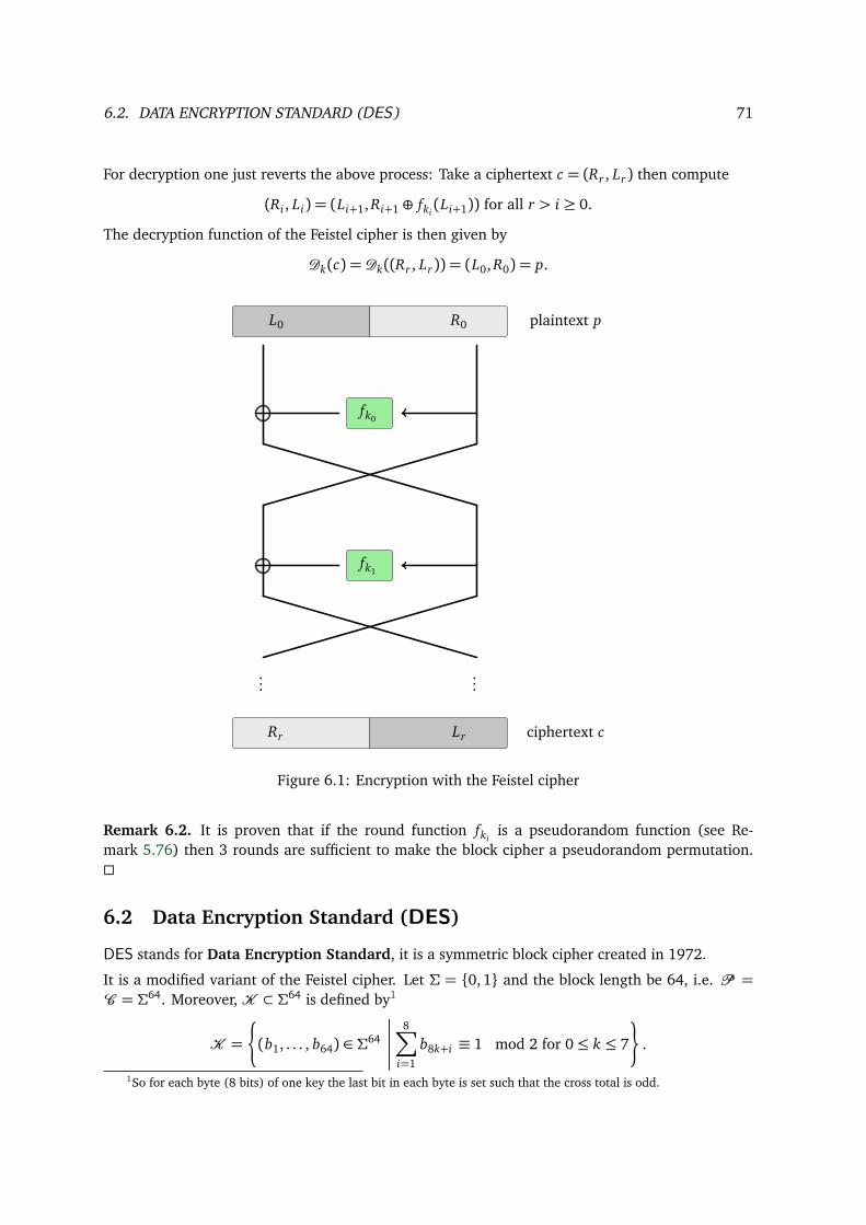
6.2. DATA ENCRYPTION STANDARD (DES) 71
For decryption one just reverts the above process: Take a ciphertext c = (Rr , Lr) then compute
(Ri , Li) = (Li+1, Ri+1 ⊕ fki(Li+1)) for all r > i ≥ 0.
The decryption function of the Feistel cipher is then given by
Dk(c) = Dk((Rr , Lr)) = (L0, R0) = p.
L0 R0 plaintext p
fk0
fk1
......
Rr Lr ciphertext c
Figure 6.1: Encryption with the Feistel cipher
Remark 6.2. It is proven that if the round function fkiis a pseudorandom function (see Re-
mark 5.76) then 3 rounds are sufficient to make the block cipher a pseudorandom permutation.
6.2 Data Encryption Standard (DES)
DES stands for Data Encryption Standard, it is a symmetric block cipher created in 1972.
It is a modified variant of the Feistel cipher. Let Σ = 0, 1 and the block length be 64, i.e. P =C = Σ64. Moreover, K ⊂ Σ64 is defined by1
K =¨(b1, . . . , b64) ∈ Σ64
8∑i=1
b8k+i ≡ 1 mod 2 for 0≤ k ≤ 7
«.
1So for each byte (8 bits) of one key the last bit in each byte is set such that the cross total is odd.
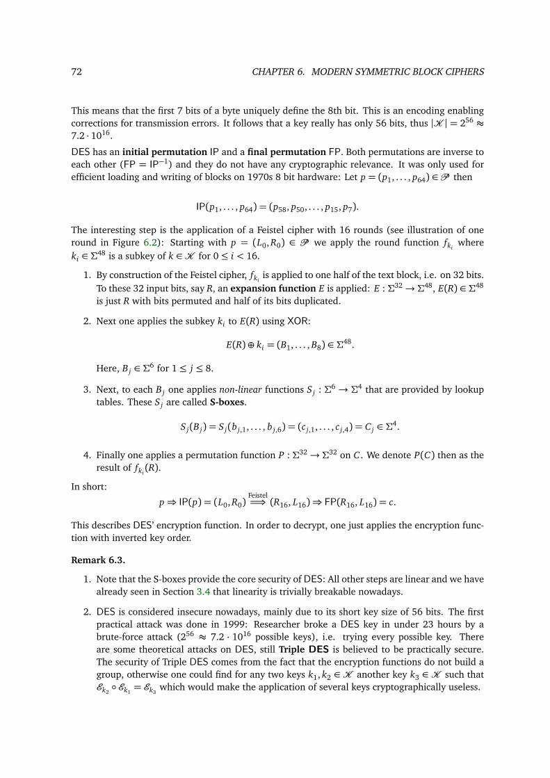
72 CHAPTER 6. MODERN SYMMETRIC BLOCK CIPHERS
This means that the first 7 bits of a byte uniquely define the 8th bit. This is an encoding enablingcorrections for transmission errors. It follows that a key really has only 56 bits, thus |K | = 256 ≈7.2 · 1016.
DES has an initial permutation IP and a final permutation FP. Both permutations are inverse toeach other (FP = IP−1) and they do not have any cryptographic relevance. It was only used forefficient loading and writing of blocks on 1970s 8 bit hardware: Let p = (p1, . . . , p64) ∈ P then
IP(p1, . . . , p64) = (p58, p50, . . . , p15, p7).
The interesting step is the application of a Feistel cipher with 16 rounds (see illustration of oneround in Figure 6.2): Starting with p = (L0, R0) ∈ P we apply the round function fki
whereki ∈ Σ48 is a subkey of k ∈K for 0≤ i < 16.
1. By construction of the Feistel cipher, fkiis applied to one half of the text block, i.e. on 32 bits.
To these 32 input bits, say R, an expansion function E is applied: E : Σ32→ Σ48, E(R) ∈ Σ48
is just R with bits permuted and half of its bits duplicated.
2. Next one applies the subkey ki to E(R) using XOR:
E(R)⊕ ki = (B1, . . . , B8) ∈ Σ48.
Here, B j ∈ Σ6 for 1≤ j ≤ 8.
3. Next, to each B j one applies non-linear functions S j : Σ6 → Σ4 that are provided by lookuptables. These S j are called S-boxes.
S j(B j) = S j(b j,1, . . . , b j,6) = (c j,1, . . . , c j,4) = C j ∈ Σ4.
4. Finally one applies a permutation function P : Σ32→ Σ32 on C . We denote P(C) then as theresult of fki
(R).
In short:
p⇒ IP(p) = (L0, R0)Feistel=⇒ (R16, L16)⇒ FP(R16, L16) = c.
This describes DES’ encryption function. In order to decrypt, one just applies the encryption func-tion with inverted key order.
Remark 6.3.
1. Note that the S-boxes provide the core security of DES: All other steps are linear and we havealready seen in Section 3.4 that linearity is trivially breakable nowadays.
2. DES is considered insecure nowadays, mainly due to its short key size of 56 bits. The firstpractical attack was done in 1999: Researcher broke a DES key in under 23 hours by abrute-force attack (256 ≈ 7.2 · 1016 possible keys), i.e. trying every possible key. Thereare some theoretical attacks on DES, still Triple DES is believed to be practically secure.The security of Triple DES comes from the fact that the encryption functions do not build agroup, otherwise one could find for any two keys k1, k2 ∈ K another key k3 ∈ K such thatEk2 Ek1
= Ek3which would make the application of several keys cryptographically useless.
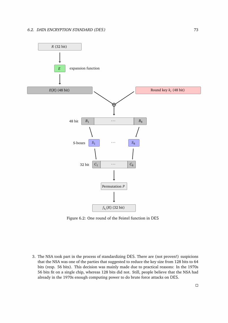
6.2. DATA ENCRYPTION STANDARD (DES) 73
R (32 bit)
E expansion function
E(R) (48 bit) Round key ki (48 bit)
· · ·B1 B848 bit
· · ·S1 S8S-boxes
· · ·C1 C832 bit
Permutation P
fki(R) (32 bit)
Figure 6.2: One round of the Feistel function in DES
3. The NSA took part in the process of standardizing DES. There are (not proven!) suspicionsthat the NSA was one of the parties that suggested to reduce the key size from 128 bits to 64bits (resp. 56 bits). This decision was mainly made due to practical reasons: In the 1970s56 bits fit on a single chip, whereas 128 bits did not. Still, people believe that the NSA hadalready in the 1970s enough computing power to do brute force attacks on DES.
74 CHAPTER 6. MODERN SYMMETRIC BLOCK CIPHERS
6.3 Advanced Encryption Standard (AES)
AES is a subset resp. specialized instantiation of the Rijndael cipher named after two Belgiancryptographers, Joan Daemen and Vincent Rijmen. AES was standardized by the U.S. NIST2 aftera process of 5 years. It was announced on 26th of November 2001.
AES, as DES, is based on substitution and permutation and is fast in software and hardware.3 Incontrast to DES, AES does not use the Feistel cipher. Let us assume the following general conceptsfor a block cipher:
Let Σ = F = F2n = F2/⟨ f ⟩ be the finite field with 2n elements. We list four different actions onB := F ℓ.
1. SubByte or S-box: The inversion in the field F defines a permutation −1 : a 7→ a−1 fora ∈ F∗ and 0−1 := 0. This permutation is non-linear but fixes 0,±1. Choose an F2-linearinvertible map g : F → F and an element t ∈ F such that σ : F → F, a 7→ ga−1 + t is a fixed-point-free permutation (or derangement). Extend σ to a permutation p = (a1, . . . , aℓ) 7→(σ(a1), . . . ,σ(aℓ)) on B.
2. ShiftRows: A permutation π ∈ Sℓ induces a block permutation on B defined by
(a1, . . . , aℓ) 7→aπ(1), . . . , aπ(ℓ)
.
3. MixColumns: Choose an element h ∈ F[x] of degree m | ℓ and an invertible element c in theresidue class ring4 R := F[x]/⟨h⟩. Then c ∈ R∗ induces a permutation c : F m→ F m, p 7→ c · p,where p = (a1, . . . , am) is identified with the polynomial am xm−1+ · · ·+a2 x+a1. Extend thispermutation to a permutation on B = F ℓ = (F m)
ℓm by p = (p1, . . . , p ℓ
m) 7→ (c · p1, . . . , c · p ℓ
m).
4. AddRoundKey: In case K = B then the addition of a key e induces a permutation p 7→ p+ eon B = F ℓ.
Note that (1) and (2) commute but (1) and (3) don’t.
The specific instantiation of AES now looks as follows:
1. n = 8: The 256 elements in the field F = F28 = F256 are considered as bytes (= 8 bits) andrepresented by two hexadecimal digits 00,01, . . . ,0F,10, . . . ,FF. As customary we write 0xin front of hexadecimal numbers. So 0x63 is the hexadecimal representation of the decimalnumber 99= 6 · 161 + 3 · 160. Its binary representation is 01100011.
2. ℓ := 16: B = F16 ∼=F2F128
2 which has more elements than atoms in the universe.
3. f := fAES := x8+x4+x3+x+1: Then 0x63 corresponds to the field element x6+ x5+ x+1 ∈ F .
2National Institute of Standards and Technology3Modern CPUs have AES functionality in hardware, e.g. for data volume encryption.4Note that we do not require R to be a field.
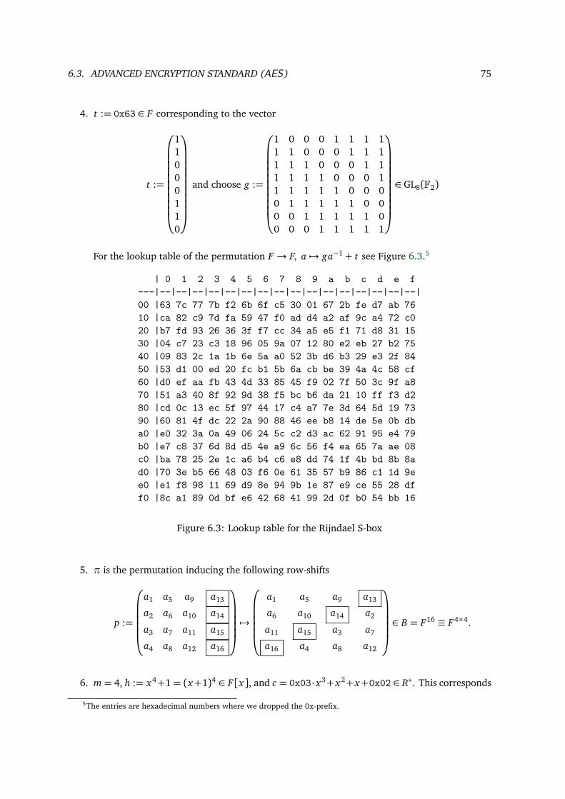
6.3. ADVANCED ENCRYPTION STANDARD (AES) 75
4. t := 0x63 ∈ F corresponding to the vector
t :=
11000110
and choose g :=
1 0 0 0 1 1 1 11 1 0 0 0 1 1 11 1 1 0 0 0 1 11 1 1 1 0 0 0 11 1 1 1 1 0 0 00 1 1 1 1 1 0 00 0 1 1 1 1 1 00 0 0 1 1 1 1 1
∈ GL8(F2)
For the lookup table of the permutation F → F, a 7→ ga−1 + t see Figure 6.3.5
| 0 1 2 3 4 5 6 7 8 9 a b c d e f---|--|--|--|--|--|--|--|--|--|--|--|--|--|--|--|--|00 |63 7c 77 7b f2 6b 6f c5 30 01 67 2b fe d7 ab 7610 |ca 82 c9 7d fa 59 47 f0 ad d4 a2 af 9c a4 72 c020 |b7 fd 93 26 36 3f f7 cc 34 a5 e5 f1 71 d8 31 1530 |04 c7 23 c3 18 96 05 9a 07 12 80 e2 eb 27 b2 7540 |09 83 2c 1a 1b 6e 5a a0 52 3b d6 b3 29 e3 2f 8450 |53 d1 00 ed 20 fc b1 5b 6a cb be 39 4a 4c 58 cf60 |d0 ef aa fb 43 4d 33 85 45 f9 02 7f 50 3c 9f a870 |51 a3 40 8f 92 9d 38 f5 bc b6 da 21 10 ff f3 d280 |cd 0c 13 ec 5f 97 44 17 c4 a7 7e 3d 64 5d 19 7390 |60 81 4f dc 22 2a 90 88 46 ee b8 14 de 5e 0b dba0 |e0 32 3a 0a 49 06 24 5c c2 d3 ac 62 91 95 e4 79b0 |e7 c8 37 6d 8d d5 4e a9 6c 56 f4 ea 65 7a ae 08c0 |ba 78 25 2e 1c a6 b4 c6 e8 dd 74 1f 4b bd 8b 8ad0 |70 3e b5 66 48 03 f6 0e 61 35 57 b9 86 c1 1d 9ee0 |e1 f8 98 11 69 d9 8e 94 9b 1e 87 e9 ce 55 28 dff0 |8c a1 89 0d bf e6 42 68 41 99 2d 0f b0 54 bb 16
Figure 6.3: Lookup table for the Rijndael S-box
5. π is the permutation inducing the following row-shifts
p :=
a1 a5 a9 a13
a2 a6 a10 a14
a3 a7 a11 a15
a4 a8 a12 a16
7→
a1 a5 a9 a13
a6 a10 a14 a2
a11 a15 a3 a7
a16 a4 a8 a12
∈ B = F16 ≡ F4×4.
6. m= 4, h := x4+1= (x+1)4 ∈ F[x], and c = 0x03·x3+x2+x+0x02 ∈ R∗. This corresponds
5The entries are hexadecimal numbers where we dropped the 0x-prefix.
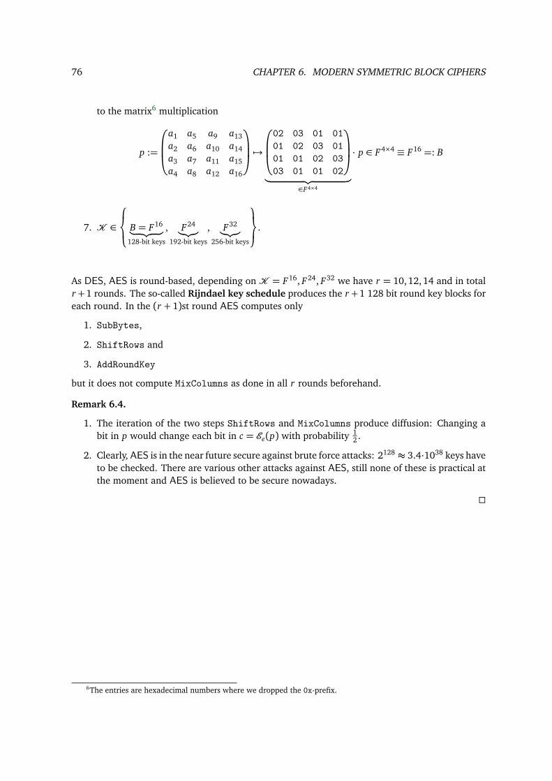
76 CHAPTER 6. MODERN SYMMETRIC BLOCK CIPHERS
to the matrix6 multiplication
p :=
a1 a5 a9 a13a2 a6 a10 a14a3 a7 a11 a15a4 a8 a12 a16
7→02 03 01 01
01 02 03 0101 01 02 0303 01 01 02
︸ ︷︷ ︸
∈F4×4
· p ∈ F4×4 ≡ F16 =: B
7. K ∈ B = F16︸ ︷︷ ︸
128-bit keys
, F24︸︷︷︸192-bit keys
, F32︸︷︷︸256-bit keys
.
As DES, AES is round-based, depending on K = F16, F24, F32 we have r = 10, 12, 14 and in totalr+1 rounds. The so-called Rijndael key schedule produces the r+1 128 bit round key blocks foreach round. In the (r + 1)st round AES computes only
1. SubBytes,
2. ShiftRows and
3. AddRoundKey
but it does not compute MixColumns as done in all r rounds beforehand.
Remark 6.4.
1. The iteration of the two steps ShiftRows and MixColumns produce diffusion: Changing abit in p would change each bit in c = Ee(p) with probability 1
2 .
2. Clearly, AES is in the near future secure against brute force attacks: 2128 ≈ 3.4·1038 keys haveto be checked. There are various other attacks against AES, still none of these is practical atthe moment and AES is believed to be secure nowadays.
6The entries are hexadecimal numbers where we dropped the 0x-prefix.
Chapter 7
Candidates of One-Way Functions
In order to construct asymmetric crypto systems we need to investigate the concept of one-wayfunctions (see Chapter 5) in more detail. First, let us recall the main complexity assumptions weneed for proving the existence of cryptographically useful one-way functions.
7.1 Complexity classes
Let us recall the main statements from our introduction to complexity theory in Section 2.1.
Definition 7.1 (see Definition 2.7). A problem instance P lies in the complexity class
1. P if P is solvable by a deterministic algorithm with polynomial runtime.
2. BPP if P is solvable by a probabilistic algorithm with polynomial runtime.
3. BQP if P is solvable by a deterministic algorithm on a quantum computer in polynomialruntime.
4. NP if P is verifiable by a deterministic algorithm with polynomial runtime.
5. NPC if any other problem in NP can be reduced resp. transformed to P in polynomial time.
6. EXP if P is solvable by a deterministic algorithm with exponential runtime.
Definition 7.2. Let G = ⟨g⟩ be a finite cyclic group. For each y ∈ G, there is exactly one minimala ∈ N0 with ga = y . We call a the discrete logarithm of y with basis g. Computing a =“logg y”(given g and y) is called the discrete logarithm problem (DLP).
Remark 7.3. In modern cryptography we make the following two standard assumptions:
1. DL assumption: DLP ∈ BPP, i.e., the computation of the discrete logarithm in the groupF∗p is not in BPP.
2. FACTORING assumption: The factorization of natural numbers does not lie in BPP.
We can prove the existence of cryptographically useful one-way functions only under such assump-tions.
77
78 CHAPTER 7. CANDIDATES OF ONE-WAY FUNCTIONS
Example 7.4. For each prime p choose a fixed primitive element a ∈ Z/pZ. Assuming DL, thefunction
f : 1, . . . , p− 1 → 1, . . . , p− 1, x 7→ ax mod p.
is a OWF with hardcore predicate
b(x) =
1 if x < p
2 ,0 if x ≥ p
2 .
7.2 Squaring modulo n
Consider the squaring homomorphism
qn : (Z/nZ)∗→ (Z/nZ)∗, x 7→ x2.
Remark 7.5.
1. If n= p is a prime then
a) ker qn = ±1.b) If p > 2 then there are exactly p−1
2 squares in (Z/pZ)∗.2. If n= pq, a product of two distinct odd primes p, q. Then
a) ker qn consists of four elements.
b) There exists exactly φ(n)4 squares in (Z/nZ)∗.
Example 7.6. Consider the following values of n:
1. n= 3:a 1 2
a2 1 1
2. n= 5:a 1 2 3 4
a2 1 4 4 1
3. n= 15:a 1 2 4 7 8 11 13 14
a2 1 4 1 4 4 1 4 1
Note that φ(15) = φ(3)φ(5) = 2 · 4= 8, and thus, φ(15)4 = 2.
Now we want to study classical methods to identify squares and compute square roots.
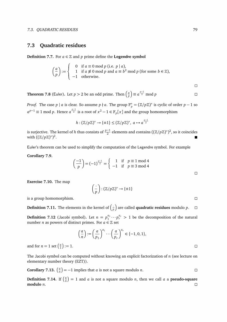
7.3. QUADRATIC RESIDUES 79
7.3 Quadratic residues
Definition 7.7. For a ∈ Z and p prime define the Legendre symbol
ap
:=
0 if a ≡ 0 mod p (i.e. p | a),1 if a ≡ 0 mod p and a ≡ b2 mod p (for some b ∈ Z),−1 otherwise.
Theorem 7.8 (Euler). Let p > 2 be an odd prime. Then
ap
≡ ap−1
2 mod p
Proof. The case p | a is clear. So assume p ∤ a. The group F∗p = (Z/pZ)∗ is cyclic of order p− 1 so
ap−1 ≡ 1 mod p. Hence ap−1
2 is a root of x2 − 1 ∈ Fp[x] and the group homomorphism
h : (Z/pZ)∗→ ±1 ≤ (Z/pZ)∗, a 7→ ap−1
2
is surjective. The kernel of h thus consists of p−12 elements and contains ((Z/pZ)∗)2, so it coincides
with ((Z/pZ)∗)2.
Euler’s theorem can be used to simplify the computation of the Legendre symbol. For example
Corollary 7.9. −1p
= (−1)
p−12 =
1 if p ≡ 1 mod 4−1 if p ≡ 3 mod 4
Exercise 7.10. The map ·p
: (Z/pZ)∗→ ±1
is a group homomorphism.
Definition 7.11. The elements in the kernel of ·
p
are called quadratic residues modulo p.
Definition 7.12 (Jacobi symbol). Let n = pa11 · · · par
r > 1 be the decomposition of the naturalnumber n as powers of distinct primes. For a ∈ Z seta
n
:=
ap1
a1 · · ·
apr
ar ∈ −1, 0, 1,
and for n= 1 set a
1
:= 1.
The Jacobi symbol can be computed without knowing an explicit factorization of n (see lecture onelementary number theory (EZT)).
Corollary 7.13. a
n
= −1 implies that a is not a square modulo n.
Definition 7.14. If a
n
= 1 and a is not a square modulo n, then we call a a pseudo-square
modulo n.
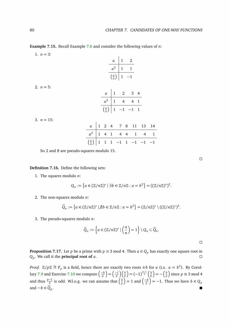
80 CHAPTER 7. CANDIDATES OF ONE-WAY FUNCTIONS
Example 7.15. Recall Example 7.6 and consider the following values of n:
1. n= 3:
a 1 2
a2 1 1 an
1 −1
2. n= 5:
a 1 2 3 4
a2 1 4 4 1 an
1 −1 −1 1
3. n= 15:
a 1 2 4 7 8 11 13 14
a2 1 4 1 4 4 1 4 1 an
1 1 1 −1 1 −1 −1 −1
So 2 and 8 are pseudo-squares modulo 15.
Definition 7.16. Define the following sets:
1. The squares modulo n:
Qn :=
a ∈ (Z/nZ)∗ | ∃b ∈ Z/nZ : a = b2= ((Z/nZ)∗)2.
2. The non-squares modulo n:
Qn :=
a ∈ (Z/nZ)∗ | ∃b ∈ Z/nZ : a = b2= (Z/nZ)∗ \ ((Z/nZ)∗)2.
3. The pseudo-squares modulo n:
eQn :=n
a ∈ (Z/nZ)∗ |a
n
= 1o\Qn ⊂Qn.
Proposition 7.17. Let p be a prime with p ≡ 3 mod 4. Then a ∈Qp has exactly one square root inQp. We call it the principal root of a.
Proof. Z/pZ ∼= Fp is a field, hence there are exactly two roots ±b for a (i.e. a = b2). By Corol-
lary 7.9 and Exercise 7.10 we compute−b
p
=−1
p
bp
= (−1)
p−12
bp
= − bp since p ≡ 3 mod 4
and thus p−12 is odd. W.l.o.g. we can assume that
bp
= 1 and−b
p
= −1. Thus we have b ∈ Qp
and −b ∈Qp.
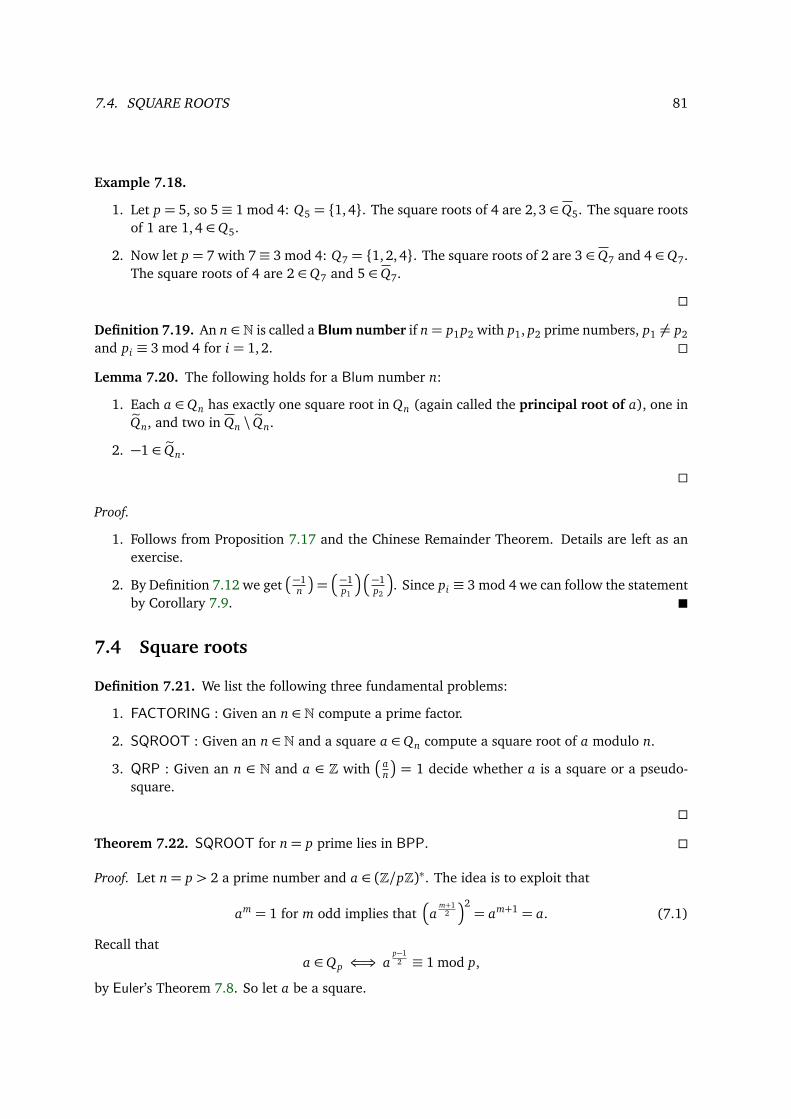
7.4. SQUARE ROOTS 81
Example 7.18.
1. Let p = 5, so 5≡ 1 mod 4: Q5 = 1, 4. The square roots of 4 are 2, 3 ∈Q5. The square rootsof 1 are 1, 4 ∈Q5.
2. Now let p = 7 with 7≡ 3 mod 4: Q7 = 1, 2, 4. The square roots of 2 are 3 ∈Q7 and 4 ∈Q7.The square roots of 4 are 2 ∈Q7 and 5 ∈Q7.
Definition 7.19. An n ∈ N is called a Blum number if n= p1p2 with p1, p2 prime numbers, p1 = p2and pi ≡ 3 mod 4 for i = 1, 2.
Lemma 7.20. The following holds for a Blum number n:
1. Each a ∈Qn has exactly one square root in Qn (again called the principal root of a), one ineQn, and two in Qn \ eQn.
2. −1 ∈ eQn.
Proof.
1. Follows from Proposition 7.17 and the Chinese Remainder Theorem. Details are left as anexercise.
2. By Definition 7.12 we get−1
n
=−1
p1
−1p2
. Since pi ≡ 3 mod 4 we can follow the statement
by Corollary 7.9.
7.4 Square roots
Definition 7.21. We list the following three fundamental problems:
1. FACTORING : Given an n ∈ N compute a prime factor.
2. SQROOT : Given an n ∈ N and a square a ∈Qn compute a square root of a modulo n.
3. QRP : Given an n ∈ N and a ∈ Z with a
n
= 1 decide whether a is a square or a pseudo-
square.
Theorem 7.22. SQROOT for n= p prime lies in BPP.
Proof. Let n= p > 2 a prime number and a ∈ (Z/pZ)∗. The idea is to exploit that
am = 1 for m odd implies thata
m+12
2= am+1 = a. (7.1)
Recall thata ∈Qp ⇐⇒ a
p−12 ≡ 1 mod p,
by Euler’s Theorem 7.8. So let a be a square.
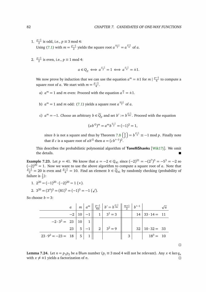
82 CHAPTER 7. CANDIDATES OF ONE-WAY FUNCTIONS
1. p−12 is odd, i.e., p ≡ 3 mod 4:
Using (7.1) with m= p−12 yields the square root a
m+12 = a
p+14 of a.
2. p−12 is even, i.e., p ≡ 1 mod 4:
a ∈Qp ⇐⇒ ap−1
2 = 1 ⇐⇒ ap−1
4 = ±1.
We now prove by induction that we can use the equation am = ±1 for m | p−14 to compute a
square root of a. We start with m= p−14 .
a) am = 1 and m even: Proceed with the equation am2 = ±1.
b) am = 1 and m odd: (7.1) yields a square root am+1
2 of a.
c) am = −1. Choose an arbitrary b ∈Qp and set b′ := bp−14m . Proceed with the equation
(ab′2)m = am bp−1
2 = (−1)2 = 1,
since b is not a square and thus by Theorem 7.8
bp
= b
p−12 ≡ −1 mod p. Finally note
that if c is a square root of ab′2 then a = (cb′−1)2.
This describes the probabilistic polynomial algorithm of TonelliShanks [Wik17j]. We omitthe details.
Example 7.23. Let p = 41. We know that a = −2 ∈ Q41 since (−2)21 = −(27)3 = −53 = −2 so(−2)20 = 1. Now we want to use the above algorithm to compute a square root of a. Note thatp−1
2 = 20 is even and p−14 = 10. Find an element b ∈ Q41 by randomly checking (probability of
failure is 12):
1. 220 = (−1)20 · (−2)20 = 1 (×).2. 320 = (34)5 = (81)5 = (−1)5 = −1 (
p).
So choose b = 3:
a m am p−14m b′ = b
p−14m m+1
2 b′−1 pa
−2 10 −1 1 31 = 3 14 33 · 14= 11
−2 · 32 = 23 10 1
23 5 −1 2 32 = 9 32 10 · 32= 33
23 · 92 = −23= 18 5 1 3 183 = 10
Lemma 7.24. Let n= p1p2 be a Blum number (pi ≡ 3 mod 4 will not be relevant). Any x ∈ ker qnwith x = ±1 yields a factorization of n.
7.5. ONE-WAY FUNCTIONS 83
Proof. Let x ∈ m ∈ N | 1< m< n−1 and m2 ≡ 1 mod n. Then p1p2 = n | x2−1= (x−1)(x+1).Since n ∤ x ± 1 we conclude w.l.o.g. that p1 | x − 1 and p2 | x + 1. Now p1 can be effectivelycomputed as p1 = gcd(x − 1, n).
Theorem 7.25. If SQROOT for Blum numbers lies in BPP then FACTORING for Blum numberslies in BPP.
Proof. From a probabilistic polynomial algorithm A that solves SQROOT for Blum numbers weconstruct the following probabilistic polynomial algorithm that solves FACTORING:Choose an arbitrary element c ∈ (Z/nZ)∗ and compute a := A(c2). So c
a is an element in ker qn
which is with probability 12 different from ±1. The rest is Lemma 7.24
7.5 One-way functions
We sharpen our previous assumption on factorization:
1. FACTORING assumption: FACTORING of Blum numbers does not lie in BPP.
2. QR assumption: QRP for Blum numbers does not lie in BPP.
Theorem 7.26. Let n be a Blum number. Then f := qn|Qn: Qn→Qn is a permutation.
1. f is a one-way permutation (OWP) under the FACTORING assumption (with security pa-rameter: k := ⌈lg |Qn|⌉=
lg φ(n)4
£= ⌈lgφ(n)⌉ − 2).
2. The so-called parity (bit)
par : (Z/nZ)∗→ 0, 1, a 7→ (smallest nonnegative representative of a)mod 2
defines under the QR assumption a hardcore bit of f .
Proof. f is a permutation by Lemma 7.20 (1) since each a ∈Qn has exactly one square root in Qn.
1. From Theorem 7.25 Statement (1) follows.
2. To prove (2) let a
n
= 1, i.e., a ∈Qn∪ eQn. For the principal root w ∈Qn of a2 we claim:
w= a ⇐⇒ par(w) = par(a). (7.2)
The forward implication of the claim is trivial. We now prove the backward implication: Since−1 ∈ eQn by Lemma 7.20 (2) and w ∈ Qn we deduce that −w ∈ eQn (i.e., that eQn = −Qn). Soa = w or a = −w. In other words: a = w =⇒ a = −w =⇒ par(w) = par(a) (remember, nas a Blum number is odd). So the above claim holds. From an algorithm B for which B(x)with x = f (a) = a2 predicts par(a) we obtain an algorithm for QRP by returning:
a is a square if B(a2) = par(w),a is a pseudo-square if B(a2) = par(w).
Due to the QR assumption such an algorithm does not lie in BPP.
84 CHAPTER 7. CANDIDATES OF ONE-WAY FUNCTIONS
Definition 7.27. The function f is called the Rabin function. The PRBG G constructed accordingto Theorem 5.73 is called the Blum-Blum-Shub generator (see [Wik17a]): For a Blum numbern and a seed s ∈ (Z/nZ)∗ define G(s) = x0 x1 x2 . . . with x i = par(s2i
). G is then a CSPRBG underthe QR assumption for Blum numbers.
7.6 Trapdoors
A OWP f : 0, 1•→ 0, 1• can be viewed as a family of permutations fk : 0, 1k→ 0, 1k.
To define a OWP with a trapdoor1 we need the following properties and structures:
1. I , an infinite index set,
2. | · | : I → N, a length function.
3. Ik := i ∈ I : |i| ≤ k (we call k the security parameter).
4. X i for all i ∈ I , a family of finite sets.
5. f = ( fi)i∈I :∪
i∈I X i →∪i∈I X i , a family of permutations fi : X i → X i .
6. A trapdoor information t i for all i ∈ I (see the examples below).
7. E , a polynomial algorithm with E (i, x) = Ei(x) = fi(x) for all i ∈ I and x ∈ X i .
8. D, a polynomial algorithm with D(i, t i , fi(x)) = D(i,t i)( fi(x)) = x for all i ∈ I and x ∈ X i .
9. Sk := (i, x) | i ∈ Ik, x ∈ X i, the possible inputs of E with security parameter k.
For a probabilistic algorithm A :∪
i∈I X i →∪i∈I X i with output A(i, y) ∈ X i for all i ∈ I and y ∈ X idefine the probabilistic algorithm A f by setting
A f (i, x) =
1 if A(i, fi(x)) = x ,0 otherwise,
for all i ∈ I and x ∈ X i .
As usual, let USkdenote the uniformly distributed random variable on Sk (i.e., first choose a random
i ∈ I and then a random x ∈ X i). Then µA f USk(1) is the probability of A correctly computing the
preimage x of y = fi(x).
Definition 7.28. The permutation f = ( fi)i∈I :∪
i∈I X i →∪i∈I X i is called a one-way permutationwith trapdoor t = (t i)i∈I if k 7→ µA f USk
(1) is negligible for all polynomial algorithms A as above(cf. Definition 5.70 (1)).
Example 7.29 (Rabin function). Set I := Blum numbers, |n| = k = ⌊lg n⌋, Xn = Qn, fn = qn|Qn:
x 7→ x2 mod n, tn the factorization of n, and D is the combination of the algorithm in the proof ofTheorem 7.22 (Tonelli-Shanks) with the Chinese Remainder Theorem. We obtain a one-way per-mutation with trapdoor under the FACTORING assumption, which is equivalent to the “SQROOT∈ BPP” assumption for Blum numbers.2 The parity bit b := par is a hardcore bit under the QRassumption (by Theorem 7.26 (2)).
1German: wörtlich Falltür, man sagt aber im Deutschen Hintertür2The equivalence is Theorem 7.22 combined with the Chinese Remainder Theorem and Theorem 7.25.
7.7. THE BLUM-GOLDWASSER CONSTRUCTION 85
7.7 The Blum-Goldwasser construction
Given a OWP with trapdoor and hardcore bit b Blum and Goldwasser constructed the followingasymmetric probabilistic3 cryptosystem (P ,C ,κ,E ,D) with
1. P =C = 0, 1•,2. K = I , K ′ = (i, t i) | i ∈ I, κ :K ′→K , (i, t i) 7→ i,
3. Ee :P C , Dd :C →P as follows (compare with Example 5.77):Let e ∈K and p ∈ 0, 1ℓ. Choose an arbitrary seed s ∈ X e and compute the sequence
r = b(s)b( fe(s)) . . . b( f ℓ−1e (s))
together with f ℓe (s) ∈ X e. Define
Ee(p) = f ℓe (s) · (p+ r),
where, as customary, + is the bitwise addition and · the concatenation4 of bits.Let now d = (e, te) ∈ K ′ and c = s′ · c′ with c′ ∈ 0, 1ℓ. Use s′ = f ℓe (s) and the trapdoorinformation te to recursively compute f ℓ−1
e (s), . . . , fe(s), s. Now compute
r = b(s)b( fe(s)) . . . b( f ℓ−1e (s))
and return Dd(c) = c′ + r.
Definition 7.30. The Blum-Goldwasser construction applied to the Rabin function is called theBlum-Goldwasser cryptosystem.
Theorem 7.31. The Blum-Goldwasser cryptosystem is an asymmetric probabilistic cryptosystemwhere
1. The FACTORING assumption implies ASYMMETRY5 (i.e., the secret key cannot be com-puted in polynomial time using the public key).
2. The QR assumption implies IND-CPA.6
Proof.
1. By definition, computing d = (n, tn) means factoring the Blum number n.
2. Let p1, p2 ∈ 0, 1ℓ and ci = Ee(pi). The QR assumption, Theorem 7.26 (2), and Theo-rem 5.73 imply that the construction of r defines a CSPRBG. Hence an attacker cannotdistinguish between p1 + r1 and p2 + r2 (even if f ℓe (s) is known; not proven here).
3Recall that for an asymmetric cryptosystem to satisfy IND it must be probabilistic with E multi-valued.4 f ℓ(s) stands for its bit-coding.5The negation of ASYMMETRY is called “total break”. This property only makes sense for public key cryptosystems.6cf. Definitions 2.24 and 2.29 and Remark 2.28
Chapter 8
Public Key Cryptosystems
Now we are ready to investigate asymmetric, i.e. public key cryptosystems in more detail. Recallwhat this means: the private key cannot be computed in polynomial time using the public key.
8.1 RSARSA was one of the first practical public key cryptosystems and is nowadays widely used. Itscreators Ron Rivest, Adi Shamir and Leonard Adleman publicly described RSA in 1977.
The main idea of RSA boils down to the following statement:
Lemma 8.1. Let n, e ∈ N with gcd(e,φ(n)) = 1. Then
fe : (Z/nZ)∗→ (Z/nZ)∗, a 7→ ae
is a permutation with inverse fd , where de ≡ 1 mod φ(n).
Proof. By definition φ(n) = |(Z/nZ)∗|. The extended Euclidian division algorithm yields the BÉ-ZOUT identity de+λφ(n) = 1. Since aφ(n) = 1 for a ∈ (Z/nZ)∗ by LAGRANGE’s theorem we concludethat
a = a1 = ade+λφ(n) = (ae)d .
Recall that for n= pq with p and q distinct primes it follows that φ(n) = (p− 1)(q− 1).
Example 8.2 (RSA function). Define the set
I := (n= pq, e) | p, q are distinct primes and gcd(e, (p− 1)(q− 1)) = 1.For i = (n= pq, e) ∈ I we define
1. fi : a 7→ ae mod n (RSA function resp. encryption).
2. de ≡ 1 mod (p− 1)(q− 1).
3. gi : y 7→ yd mod n (inverse function resp. decryption).
86
8.1. RSA 87
Definition 8.3. The RSA problem (RSAP) is the problem of inverting the RSA function. TheRSA assumption is that RSAP ∈ BPP.
Remark 8.4.
1. The RSAP reduces to FACTORING, i.e., the RSA assumption is stronger than the FACTOR-ING assumption.
2. Under the RSA assumption: The RSA function is a OWP with trapdoor and hardcore bitb = par (parity bit; without proof). The Blum-Goldwasser construction yields, as for theRabin function, a probabilistic asymmetric cryptosystem satisfying IND-CPA .
Definition 8.5. The RSA cryptosystem is defined as follows: For a given n ∈ N>0 we define
1. Pn = 0, 1k, C = 0, 1k+1 where k = ⌊lg n⌋.2. Kn = I = (n= pq, e) | p, q are distinct primes and gcd(e, (p− 1)(q− 1)) = 1 as above.
3. K ′n = (n= pq, d, e) | p, q distinct primes, |p|, |q| ≈ k2 , |pq| ≥ k, de ≡ 1 mod φ(n).
4. κn : (n, d, e) 7→ (n, e) ∈K .
5. E(n,e)(x) = x e mod n.
6. D(n,d,e)(y) = yd mod n.
Note that in practice one defines a security level k and then defines based on this p, q, and n.
Remark 8.6. We now list the security properties of the RSA cryptosystem (assuming a CPA attack,which is natural for public cryptosystems):
1. p, q and φ(n) must remain secret.
2. RSA assumption =⇒ OW =⇒ ASYMMETRY.
3. IND is not satisfied since the cryptosystem is deterministic.
4. NM is not satisfied since the cryptosystem is multiplicative: (ab)e = ae be (see below).
Example 8.7. Let p = 11, q = 23, and e = 3. Then n = pq = 253, k = ⌊lg n⌋ = 7, φ(n) =(p−1)(q−1) = 10·22= 220, and d = 147 with ed = 441≡ 1 mod 220. For m= 0110100= (52)10we compute
c = E(n,e)(m) = 523 = 193 mod 253= (1100001)2.
Now we decrypt viaD(253,147,3)(c) = 193147 ≡ 52 mod 253= m.
Violating the NM: To shift m one position to the left we manipulate c to c′ = E(253,3)(2) · c =23 · 193= 26 mod 253. Then D(253,147,3)(c) = 26147 ≡ 104 mod 253= (1101000)2.
In analogy with the trivial statement of Theorem 7.31.(1) for the Blum-Goldwasser cryptosystemwe prove:
88 CHAPTER 8. PUBLIC KEY CRYPTOSYSTEMS
Theorem 8.8. The FACTORING assumption implies the ASYMMETRY of the RSA cryptosystem,i.e., the secret key d cannot be computed in polynomial time using the public key (n, e).
Proof. Assume that we can compute the secret key d in polynomial time. We need to show that wecan then also factor n using the knowledge of (n, d, e) ∈K ′:The Chinese Remainder Theorem provides an isomorphism
(Z/nZ)∗→ (Z/pZ)∗ × (Z/qZ)∗, a mod n 7→ (a mod p, a mod q).
In particular ord(Z/nZ)∗(a) = lcm(ord(Z/pZ)∗(a), ord(Z/qZ)∗(a)). The idea is to use the followingtrivial equivalence
c ≡ 1 mod p, c ≡ 1 mod q ⇐⇒ n> gcd(c − 1, n) = p > 1.
to factor n. So our goal is to construct such an element c.For any a we have that
ord(Z/pZ)∗(a) | p− 1,ord(Z/qZ)∗(a) | q− 1, andord(Z/nZ)∗(a) | (p− 1)(q− 1) = φ(n) | ed − 1.
Write ed − 1 = 2s t with t odd. Then (at)2s= 1, hence ord(Z/nZ)∗(at) | 2s. Choose randomly an
element a ∈ (Z/nZ)∗ and set b := at . Then
ord(Z/pZ)∗(b) = 2i and ord(Z/qZ)∗(b) = 2 j with i, j ≤ s.
If i = j, or w.l.o.g. i < j, then c := b2i ≡ 1 mod p and c ≡ 1 mod q and we get the factorization
p = gcd(c − 1, n).
We now prove that i = j for (at least) half of all a ∈ (Z/nZ)∗ (recall, b := at). The choice of aprimitive element g ∈ (Z/pZ)∗ yields an isomorphism (Z/(p − 1)Z,+) → (Z/pZ)∗, x 7→ g x . Asabove, ord(Z/(p−1)Z,+)(1) = p− 1 | 2s t and ord(Z/(p−1)Z,+)(t) | 2s. Using the identification
(Z/nZ)∗ ∼= (Z/pZ)∗ × (Z/qZ)∗ ∼= (Z/(p− 1)Z,+)× (Z/(q− 1)Z,+)
it is thus equivalent to show that the inequality ord(Z/(p−1)Z,+)(x t) = ord(Z/(q−1)Z,+)(y t) holds for(at least) half of all pairs (x , y) ∈ (Z/(p−1)Z,+)×(Z/(q−1)Z,+): Let ord(Z/(p−1)Z,+)(t) = 2k andord(Z/(q−1)Z,+)(t) = 2ℓ. Note that
ord(Z/(p−1)Z,+)(t) = ord(Z/(p−1)Z,+)(x t) for all x odd (trivial).ord(Z/(p−1)Z,+)(t) > ord(Z/(p−1)Z,+)(x t) for all x even (trivial).
Clearly, the same holds for y and q− 1.
Now we distinguish two cases:
k = ℓ: Again, w.l.o.g. let ℓ < k. Then for all (x , y) with x odd we obtain:
ord(Z/(q−1)Z,+)(y t)≤ ord(Z/(q−1)Z,+)(t) = 2ℓ < 2k = ord(Z/(p−1)Z,+)(t) = ord(Z/(p−1)Z,+)(x t).
So this inequality holds for at least half of the pairs (x , y), namely those where x is odd.
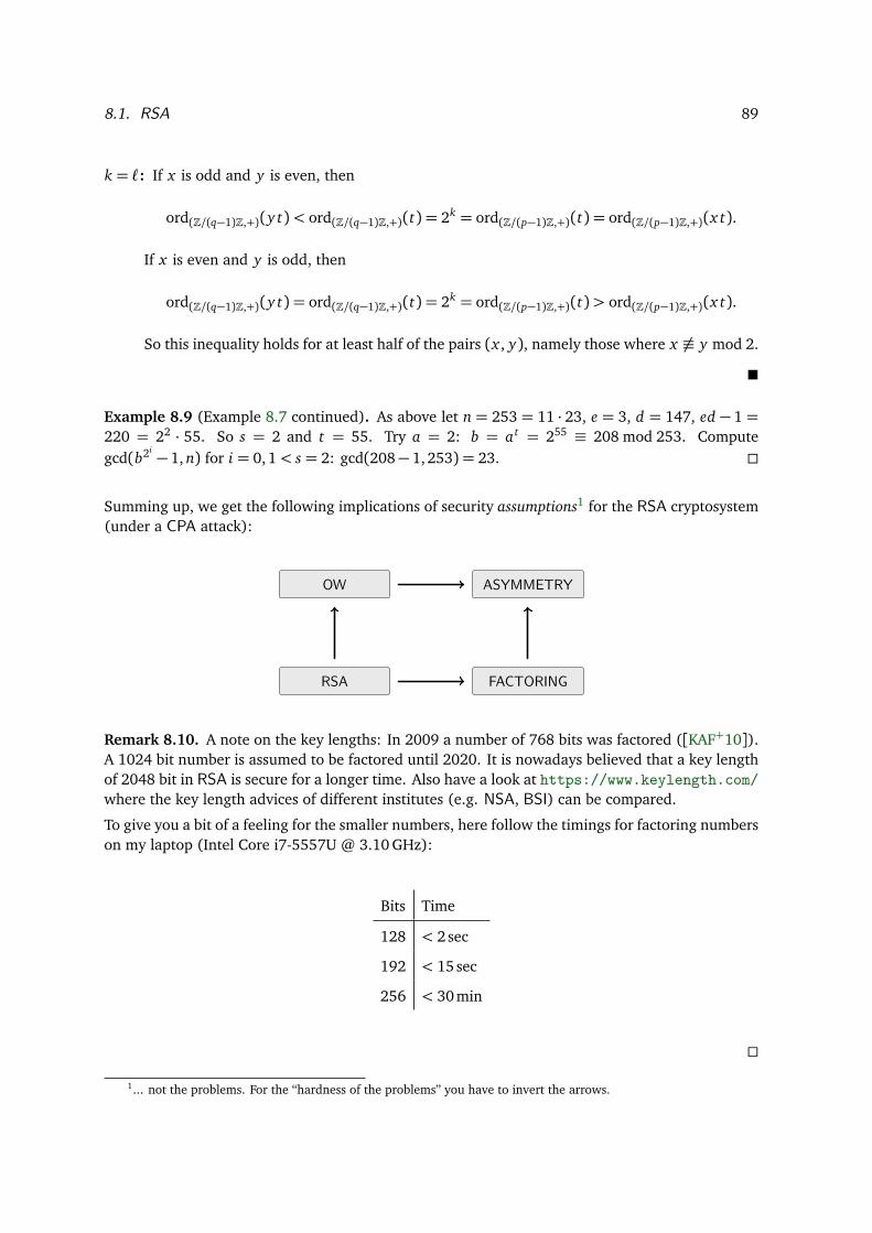
8.1. RSA 89
k = ℓ: If x is odd and y is even, then
ord(Z/(q−1)Z,+)(y t)< ord(Z/(q−1)Z,+)(t) = 2k = ord(Z/(p−1)Z,+)(t) = ord(Z/(p−1)Z,+)(x t).
If x is even and y is odd, then
ord(Z/(q−1)Z,+)(y t) = ord(Z/(q−1)Z,+)(t) = 2k = ord(Z/(p−1)Z,+)(t)> ord(Z/(p−1)Z,+)(x t).
So this inequality holds for at least half of the pairs (x , y), namely those where x ≡ y mod 2.
Example 8.9 (Example 8.7 continued). As above let n = 253 = 11 · 23, e = 3, d = 147, ed − 1 =220 = 22 · 55. So s = 2 and t = 55. Try a = 2: b = at = 255 ≡ 208 mod 253. Computegcd(b2i − 1, n) for i = 0, 1< s = 2: gcd(208− 1, 253) = 23.
Summing up, we get the following implications of security assumptions1 for the RSA cryptosystem(under a CPA attack):
RSA FACTORING
OW ASYMMETRY
Remark 8.10. A note on the key lengths: In 2009 a number of 768 bits was factored ([KAF+10]).A 1024 bit number is assumed to be factored until 2020. It is nowadays believed that a key lengthof 2048 bit in RSA is secure for a longer time. Also have a look at https://www.keylength.com/where the key length advices of different institutes (e.g. NSA, BSI) can be compared.
To give you a bit of a feeling for the smaller numbers, here follow the timings for factoring numberson my laptop (Intel Core i7-5557U @ 3.10 GHz):
Bits Time
128 < 2 sec
192 < 15 sec
256 < 30 min
1... not the problems. For the “hardness of the problems” you have to invert the arrows.
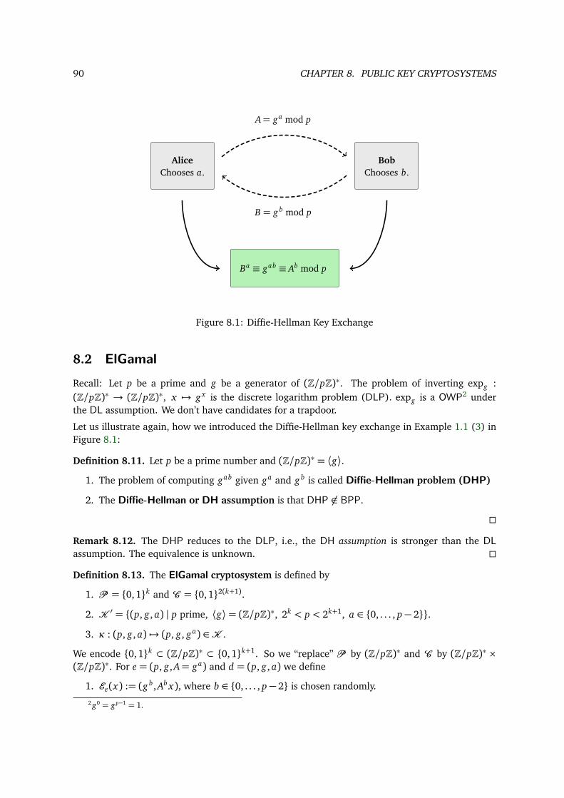
90 CHAPTER 8. PUBLIC KEY CRYPTOSYSTEMS
AliceChooses a.
BobChooses b.
A= ga mod p
B = g b mod p
Ba ≡ gab ≡ Ab mod p
Figure 8.1: Diffie-Hellman Key Exchange
8.2 ElGamalRecall: Let p be a prime and g be a generator of (Z/pZ)∗. The problem of inverting expg :(Z/pZ)∗ → (Z/pZ)∗, x 7→ g x is the discrete logarithm problem (DLP). expg is a OWP2 underthe DL assumption. We don’t have candidates for a trapdoor.
Let us illustrate again, how we introduced the Diffie-Hellman key exchange in Example 1.1 (3) inFigure 8.1:
Definition 8.11. Let p be a prime number and (Z/pZ)∗ = ⟨g⟩.1. The problem of computing gab given ga and g b is called Diffie-Hellman problem (DHP)
2. The Diffie-Hellman or DH assumption is that DHP ∈ BPP.
Remark 8.12. The DHP reduces to the DLP, i.e., the DH assumption is stronger than the DLassumption. The equivalence is unknown.
Definition 8.13. The ElGamal cryptosystem is defined by
1. P = 0, 1k and C = 0, 12(k+1).
2. K ′ = (p, g, a) | p prime, ⟨g⟩= (Z/pZ)∗, 2k < p < 2k+1, a ∈ 0, . . . , p− 2.3. κ : (p, g, a) 7→ (p, g, ga) ∈K .
We encode 0, 1k ⊂ (Z/pZ)∗ ⊂ 0, 1k+1. So we “replace” P by (Z/pZ)∗ and C by (Z/pZ)∗ ×(Z/pZ)∗. For e = (p, g, A= ga) and d = (p, g, a) we define
1. Ee(x) := (g b, Ab x), where b ∈ 0, . . . , p− 2 is chosen randomly.
2 g0 = g p−1 = 1.
8.3. THE RABIN CRYPTOSYSTEM 91
2. Dd(y, z) := y−az.
Of course, a has to be kept secret.
Proof of correctness. y−az = (g b)−aAb x = g−ba+ab x = x .
Example 8.14. Take p = 23 and g = 7. For a = 6, i.e., d = (23, 7, 6) compute A= 76 ≡ 4 mod 23.e = κ(d) = (23, 7, 4). For x = 7 ∈ (Z/23Z)∗ =P compute Ee(x) for different b’s:
1. b = 3: Ee(x) = (73, 43 · 7) = (21, 11) ∈ (Z/23Z)∗ × (Z/23Z)∗ =C .
2. b = 2: Ee(x) = (72, 42 · 7) = (3, 20) ∈ (Z/23Z)∗ × (Z/23Z)∗ =C .
Now verify Dd(21, 11) = 21−6 · 11≡ 7 mod 23≡ 3−6 · 20= Dd(3, 20).
Remark 8.15. The ElGamal cryptosystem is a probabilistic public key cryptosystem with multi-valued E . Note the following:
1. It satisfies the IND-CPA security model under the DL assumption (without proof).
2. It does not satisfy NM because of its multiplicativity (like RSA, cf. Remark 8.6).
Theorem 8.16. Under a CPA attack the (probabilistic public key) ElGamal cryptosystem satisfies
1. OW under the DH assumption.
2. ASYMMETRY under the DL assumption.
Proof.
1. Assume we can decrypt ciphertexts, i.e., from the public key information ga and the ciphertext(g b, gab x) we can compute x . Then we can in particular decrypt (g b, 1) to obtain g−ab andhence gab. This contradicts the DH assumption.
2. If a CPA adversary (i.e., who has full access to A = ga and Ee) can compute the secret keyinformation a, then she has already solved the DLP.
8.3 The Rabin cryptosystem
Next we recall the Rabin function from Definition 7.27 and Example 7.29. We look into the non-unique decryption process in more detail.
Definition 8.17. The Rabin cryptosystem is defined as follows:
1. P = 0, 1k and C = 0, 1k+1.
2. K ′ = (p, q) | p, q distinct primes, p, q ≡ 3 mod 4, 2k < pq < 2k+1.3
3. κ : (p, q) 7→ pq ∈K = n ∈ N | 2k < n< 2k+1 a Blum number.
3Note that one can show that K ′ is not empty for “reasonable” choices of k.
92 CHAPTER 8. PUBLIC KEY CRYPTOSYSTEMS
We encode 0, 1k ⊂ Z/nZ ⊂ 0, 1k+1. So we “replace”P andC by Z/nZ. For e = n and d = (p, q)we define
1. Ee(x) := x2 mod n (not injective!)
2. Dd(y) := the four square roots of x2 mod n (not uniquely determined!) using the ChineseRemainder Theorem and the simple case “p ≡ 3 mod 4” in the Tonelli-Shanks algorithm fromthe proof of Theorem 7.22.
Note that the Rabin cryptosystem is not the Blum-Goldwasser cryptosystem from Definition 7.30.
Example 8.18. Take p = 3 and q = 7. Then n = 21 is the public key of the Rabin cryptosystem.To encrypt the plain text m= 10 ∈ Z/21Z we compute
c = m2 = 102 ≡ 16 mod 21.
To decrypt c = 16 using the secret prime factors p = 3 and q = 7 we compute the four square rootsof 16 modulo 21 using the Tonelli-Shanks algorithm from Theorem 7.22: We have
16p+1
4 = 16≡ 1 mod 3 and 16q+1
4 = 162 ≡ 4 mod 7.
Hence
1. 1 and −1≡ 2 mod 3 are the square roots of 16 modulo 3.
2. 4 and −4≡ 3 mod 7 are the square roots of 16 modulo 7.
With the Chinese Remainder Theorem we get the four combinations
(1, 4), (1, 3), (2, 4), (2, 3)
and finally the four square roots4, 10, 11, 17,
among which we search for the (hopefully unique) human readable “plain text” 10.
Theorem 8.19. For the Rabin cryptosystem the following implications of assumptions hold (undera CPA attack)
FACTORING =⇒ OW =⇒ ASYMMETRY.
Proof. If we can decrypt ciphertexts we can choose random elements x ∈ Z/nZ and computesquare roots of x2. By Theorem 7.25 we then obtain a factorization of n, so a total break of thecryptosystem. This proves the first implication. The second implication is trivial.
Remark 8.20. One “problem” of the Rabin cryptosystem is the decryption which is in general notunique and a contextual search needs to be done. Note that restricting P to Qn does not eliminatethe non-uniqueness issue: It is then not clear how to find an injective encoding 0, 1k→Qn?
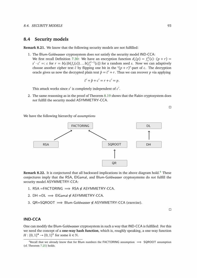
8.4. SECURITY MODELS 93
8.4 Security models
Remark 8.21. We know that the following security models are not fulfilled:
1. The Blum-Goldwasser cryptosystem does not satisfy the security model IND-CCA:We first recall Definition 7.30: We have an encryption function Ee(p) = f ℓe (s) · (p + r) =s′ · c′ =: c for r = b(s)b( fe(s)) . . . b( f ℓ−1
e (s)) for a random seed s. Now we can adaptivelychoose another cipher text c by flipping one bit in the “(p + r)”-part of c. The decryptionoracle gives us now the decrypted plain text p = c′ + r. Thus we can recover p via applying
c′ + p+ c′ = r + c′ = p.
This attack works since s′ is completely independent of c′.2. The same reasoning as in the proof of Theorem 8.19 shows that the Rabin cryptosystem does
not fulfill the security model ASYMMETRY-CCA.
We have the following hierarchy of assumptions
FACTORING
RSA SQROOT
QR
DH
DL
Remark 8.22. It is conjectured that all backward implications in the above diagram hold.4 Theseconjectures imply that the RSA, ElGamal, and Blum-Goldwasser cryptosystems do not fulfill thesecurity model ASYMMETRY-CCA:
1. RSA =FACTORING =⇒ RSA ∈ ASYMMETRY-CCA.
2. DH =DL =⇒ ElGamal ∈ ASYMMETRY-CCA.
3. QR=SQROOT =⇒ Blum-Goldwasser ∈ ASYMMETRY-CCA (exercise).
IND-CCAOne can modify the Blum-Goldwasser cryptosystem in such a way that IND-CCA is fulfilled: For thiswe need the concept of a one-way hash function, which is, roughly speaking, a one-way functionH : 0, 1•→ 0, 1k for some k ∈ N.
4Recall that we already know that for Blum numbers the FACTORING assumption =⇒ SQROOT assumption(cf. Theorem 7.25) holds.
94 CHAPTER 8. PUBLIC KEY CRYPTOSYSTEMS
Remark 8.23. The modified Blum-Goldwasser cryptosystem (cf. Definition 7.30)
Ee(p) = f ℓe (s+H(y)) · (p+ r)︸ ︷︷ ︸y
now satisfies, under the QR assumption, the security model IND-CCA. Thus we cannot apply anattack as done in Remark 8.21 any longer: s′ = f ℓe (s+H(y)) now depends on c′ = p+ r = y .
Optimal Asymmetric Encryption Padding (OAEP)
We now describe the so-called optimal asymmetric encryption padding5 (OAEP) [Wik16d]which is often used to improve the security of public key cryptosystems by preprocessing plain-texts prior to the asymmetric encryption:
1. Fix a security parameter k ∈ N.
2. Fix k0, k1 ∈ N with n := k− k0 − k1 > 0.
3. Fix a CSPRBGG : 0, 1k0 → 0, 1n+k1 .
4. Fix a one-way hash functionH : 0, 1n+k1 → 0, 1k0 ,
called the compression function.
For an n-bit plaintext p and seed s ∈ 0, 1k0 return the k-bit concatenated string
p′ =
(p · 0 . . . 0︸ ︷︷ ︸k1
) + G(s)
︸ ︷︷ ︸
=:y∈0,1n+k1
· (s+H(y)).
Now one can apply the OWP f : 0, 1k→ 0, 1k of public key cryptosystem to the padded messagep′.
Definition 8.24. The probabilistic public key cryptosystem obtained by applying the RSA functionto an OAEP-preprocessed message p′ is called the RSA-OAEP cryptosystem.
Assuming the existence of a so-called ideal compression function H one can prove that
Theorem 8.25. The RSA-OAEP cryptosystem satisfies the security model IND-CCA under the RSAassumption.
5German: Polsterung
Chapter 9
Primality tests
In the last chapter we have seen that many public key cryptosystems are based on the fact of findingbig prime factors. In this chapter we want to study various sorts of probabilistic and deterministicprimality test. Let us denote by P ⊂ N the set of prime numbers.
9.1 Probabilistic primality tests
Fermat test
Recall Fermat’s little theorem:1
Theorem 9.1. For p ∈ P it holds that ap−1 ≡ 1 mod p for all a ∈ Z \ pZ.
This yields the so-called Fermat test, an elementary probabilistic test for primality, which lies inO (log log log n):
Let n ∈ N. If there exists a ∈ (Z/nZ)∗ with an−1 ≡ 1 mod n then n is not a prime.
Note that finding an a ∈ Nn := ((Z/nZ) \ 0) \ (Z/nZ)∗ is hopeless if n is the product of hugeprimes (compare n= |Z/nZ| and n−φ(n) = |Nn|+ 1).
Example 9.2. Let n= 341. For
1. a = 2: 2340 ≡ 1 mod 341.
2. a = 3: 3340 ≡ 56 mod 341.
Hence, 341 is a composite number and 3 is a witness.2
Definition 9.3. Let n ∈ N and a ∈ (Z/nZ)∗.1. n is called a pseudoprime with Fermat nonwitness a if an−1 ≡ 1 mod n, i.e., the Fermat
test of the primality of n passes for a.
2. If n is a pseudoprime with Fermat nonwitness a but not prime then a is called a Fermat liar.
3. If the Fermat test of the primality of n fails for a, i.e., if an−1 ≡ 1 mod n, then a is called aFermat witness (for the compositeness) of n.
1This is a special case of Euler’s Theorem aφ(n) ≡ 1 mod n, for the case n= p ∈ P.2German: Zeuge.
95
96 CHAPTER 9. PRIMALITY TESTS
4. n is called a Carmichael number if n is a composite number without a Fermat witness, i.e.,if all a ∈ (Z/nZ)∗ are Fermat liars.
Of course, each prime is a pseudoprime for all a ∈ (Z/nZ)∗. In 1994 it was proven in [AGP94] thatthe set of Carmichael numbers is infinite:
561= 3 · 11 · 17, 1105= 5 · 13 · 17, 1729= 7 · 13 · 19, . . .
Lemma 9.4. Let n be a Carmichael number and p ∈ P. Then the following statements hold:
1. n is odd.
2. n is square free.
3. p | n =⇒ p− 1 | n− 1.
4. n has at least 3 prime factors.
Proof.
1. n even =⇒ n− 1 odd nCarmichael
+3 −1 = (−1)n−1 = 1 ∈ (Z/nZ)∗ =⇒ n = 2 prime (since 2
as a prime is not Carmichael).
2. Write n= pe · n′, where e is the maximal p-power. Then
φ(n) = φ(pe)φ(n′) = pe−1(p− 1)φ(n′).
Assume that p2 | n. Then it follows:
a) p | φ(n) = |(Z/nZ)∗| =⇒ ∃a ∈ (Z/nZ)∗ with ord(Z/nZ)∗(a) = p.
b) p | n =⇒ p ∤ n− 1ord(a)=p=⇒ an−1 ≡ 1 mod n =⇒ a is a Fermat witness for n =⇒ n is
not a Carmichael number.
3. Let p be a prime divisor of n. Since an−1 ≡ 1 mod n it follows that an−1 ≡ 1 mod p, for alla ∈ Z with gcd(a, n) = 1. Since (Z/pZ)∗ is cyclic, we can choose a to be a primitive element.Thus ord a = |(Z/pZ)∗|. Thus we deduce that p− 1= |(Z/pZ)∗| | n− 1.
4. Clearly, n must have more than one prime factor. Suppose n has two prime factors, n = pq,p, q ∈ P. W.l.o.g. p > q since n is square free. Then p − 1 > q − 1, so p − 1 does not divideq− 1. Now
(n− 1)− (q− 1) = n− q = pq− q = (p− 1)q.
Since p−1 does not divide q−1 it also cannot divide n−1. Since p divides n this contradicts(3) thus n is not a Carmichael number.
The existence of infinitely many Carmichael numbers means that we cannot trust the Fermat pri-mality test (unless of course it produces a Fermat witness).
9.1. PROBABILISTIC PRIMALITY TESTS 97
Miller-Rabin test
The Miller-Rabin test makes use of the fact that the equation a2 = 1 has exactly two solutionsa = ±1 over Z/nZ if n is a prime (since then Z/nZ is a field). The general idea is to improve theFermat test by successively dividing the power of a chosen element a by 2 and test again, startingwith an−1.
Lemma 9.5 (Miller-Rabin). Let p ∈ P and let a ∈ (Z/pZ)∗. Write p − 1 = 2s t with t odd (s ≥ 0).Then
at ≡ ±1 mod p or
a2r t ≡ −1 mod p for some 0< r < s.
Proof. Let 0 ≤ s0 ≤ s minimal with a2s0 t ≡ 1 mod p (recall that ap−1 ≡ 1 mod p). We distinguishtwo cases:
1. If s0 = 0 then at ≡ 1 mod p.
2. If s0 > 0 then a2r t ≡ −1 mod p with r = s0 − 1 ∈ 0, . . . , s− 1.
Definition 9.6. Let n be a composite number. Write n− 1 = 2s t with t odd (s ≥ 0). a ∈ (Z/nZ)∗is called a Miller-Rabin nonwitness if
at ≡ ±1 mod n or (±1)
a2r t ≡ −1 mod n for some 0< r < s, (−1)
otherwise a is called a Miller-Rabin witness (for the compositeness of n).
Example 9.7. Consider n= 561: n−1= 560= 24 ·35, so s = 4 and t = 35. For a = 2 we compute
235 ≡ 263 mod 561 ≡ 1,−1 mod 561
22·35 ≡ 166 mod 56124·35 ≡ 67 mod 56128·35 ≡ 1 mod 561
≡ −1 mod 561
So a = 2 is a Miller-Rabin witness for Carmichael number 561.
Remark 9.8. If the generalized Riemann hypothesis holds, then n is a prime if one of the con-ditions (±1) or (−1) is fulfilled for each 1 < a < 2 log2 n. This turns the probabilistic Miller-Rabintest into a deterministic one. See Remark 9.13 below.
Definition 9.9. For a fixed n ∈ N define
N := Miller-Rabin nonwitness for n ⊂ (Z/nZ)∗.
98 CHAPTER 9. PRIMALITY TESTS
The idea is to find a subgroup U ≤ (Z/nZ)∗ with N ⊂ U and to bound the index (Z/nZ)∗ : U frombelow away from 1. A natural candidate would be
U0 := a ∈ (Z/nZ)∗ | an−1 ≡ 1 mod n= Fermat nonwitness= ker(x 7→ xn−1)≤ (Z/nZ)∗.But we know that the index (Z/nZ)∗ : U0 might be 1:
U0 = (Z/nZ)∗ ⇐⇒ n is a prime or a Carmichael number.
Lemma 9.10. Let n= pα for α≥ 2. Then (Z/nZ)∗ : U0 ≥ p.
Proof. p | pα−1(p − 1) = φ(n) = |(Z/nZ)∗|. Then there exists an a ∈ (Z/nZ)∗ with ord(a) = p.Furthermore, p | n =⇒ p ∤ n−1 =⇒ an−1 ≡ 1 mod n =⇒ a ∈ U0. The same holds for a2, . . . , ap−1.Hence U0, aU0, a2U0, . . . , ap−1U0 ∈ (Z/nZ)∗/U0 are pairwise different and (Z/nZ)∗ : U0 ≥ p.
Theorem 9.11. Let n be a composite odd number with 3 ∤ n. Then |N | ≤ φ(n)4 < n4 .
Proof. Again write n − 1 = 2s t with t odd (s ≥ 1). Set N−1 := a ∈ N | at ≡ 1 mod n andNi := a ∈ N | a2i t ≡ −1 mod n for 0 ≤ i < s. Then N =
∪s−1i=−1 Ni = ; (since −1 ∈ N0 = ;). Set
r :=maxi | Ni = ; ∈ 0, . . . , s−1 and m := 2r t. In particular, m | n−12 =
2s t2 (because r < s). For
all a ∈ N it holds:
am ≡ −1 if a ∈ Nr ,
1 if a ∈ Ni for i < r.(9.1)
Consider the group endomorphism f : (Z/nZ)∗ → (Z/nZ)∗, a 7→ am. Let n = pα11 · · · pαu
u be thefactorization of n as the product of distinct prime powers. The Chinese Remainder Theorem yieldsthe isomorphism
(Z/nZ)∗ ∼= (Z/pα11 Z)
∗ × · · · × (Z/pαuu Z)∗,
identifying a ∈ (Z/nZ)∗ with the u-tuple (a mod pα11 , . . . , a mod pαu
u ). We now use this isomorphismto define the following chain of subgroups
(Z/nZ)∗
≤
U0 := ker(x 7→ xn−1) = a ∈ (Z/nZ)∗ | an−1 ≡ 1 mod n,
≤
U1 := f −1((±1, . . . ,±1)) = a ∈ (Z/nZ)∗ | am ≡ ±1 mod pαii , 1≤ i ≤ u
≤
U2 := f −1(±1) = a ∈ (Z/nZ)∗ | am ≡ ±1 mod n,
≤
U3 := f −1(1) = a ∈ (Z/nZ)∗ | am ≡ 1 mod n.U1 is a subgroup of U0 since m | n−1
2 (see above). The remaining inclusions are obvious as the preim-ages of inclusions of a chain of subgroups. Since N ⊂ U2 we want to bound the index (Z/nZ)∗ : U2from below away from 1. We claim that
(Z/nZ)∗ : U2 ≥ 4.
To see this we first have to prove that (±1, . . . ,±1) ≤ im f as a subgroup:Choose a b ∈ Nr = ;, then f (b) = bm ≡ −1 mod n, hence, bm ≡ −1 mod pαi
i for all i = 1, . . . , u.
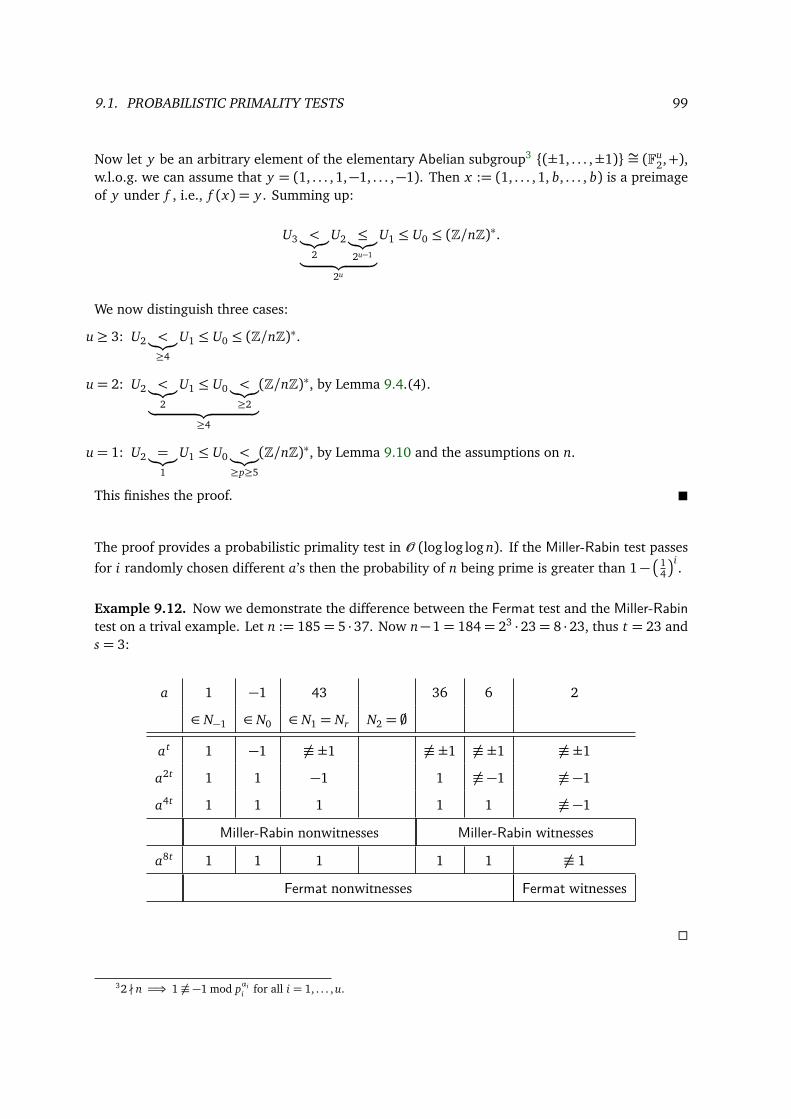
9.1. PROBABILISTIC PRIMALITY TESTS 99
Now let y be an arbitrary element of the elementary Abelian subgroup3 (±1, . . . ,±1) ∼= (Fu2,+),
w.l.o.g. we can assume that y = (1, . . . , 1,−1, . . . ,−1). Then x := (1, . . . , 1, b, . . . , b) is a preimageof y under f , i.e., f (x) = y . Summing up:
U3 <︸︷︷︸2
U2 ≤︸︷︷︸2u−1︸ ︷︷ ︸
2u
U1 ≤ U0 ≤ (Z/nZ)∗.
We now distinguish three cases:
u≥ 3: U2 <︸︷︷︸≥4
U1 ≤ U0 ≤ (Z/nZ)∗.
u= 2: U2 <︸︷︷︸2
U1 ≤ U0 <︸︷︷︸≥2︸ ︷︷ ︸
≥4
(Z/nZ)∗, by Lemma 9.4.(4).
u= 1: U2 =︸︷︷︸1
U1 ≤ U0 <︸︷︷︸≥p≥5
(Z/nZ)∗, by Lemma 9.10 and the assumptions on n.
This finishes the proof.
The proof provides a probabilistic primality test in O (log log log n). If the Miller-Rabin test passesfor i randomly chosen different a’s then the probability of n being prime is greater than 1− 14i .Example 9.12. Now we demonstrate the difference between the Fermat test and the Miller-Rabintest on a trival example. Let n := 185= 5 ·37. Now n−1= 184= 23 ·23= 8 ·23, thus t = 23 ands = 3:
a 1 −1 43 36 6 2
∈ N−1 ∈ N0 ∈ N1 = Nr N2 = ;at 1 −1 ≡ ±1 ≡ ±1 ≡ ±1 ≡ ±1
a2t 1 1 −1 1 ≡ −1 ≡ −1
a4t 1 1 1 1 1 ≡ −1
Miller-Rabin nonwitnesses Miller-Rabin witnesses
a8t 1 1 1 1 1 ≡ 1
Fermat nonwitnesses Fermat witnesses
32 ∤ n =⇒ 1 ≡ −1 mod pαii for all i = 1, . . . , u.
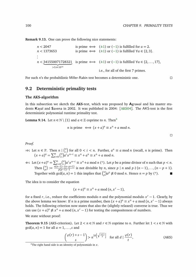
100 CHAPTER 9. PRIMALITY TESTS
Remark 9.13. One can prove the following nice statements:
n< 2047 is prime ⇐⇒ (±1) or (−1) is fulfilled for a = 2.n< 1373653 is prime ⇐⇒ (±1) or (−1) is fulfilled ∀a ∈ 2, 3....n< 341550071728321︸ ︷︷ ︸
>3.4·1014
is prime ⇐⇒ (±1) or (−1) is fulfilled ∀a ∈ 2, . . . , 17,i.e., for all of the first 7 primes.
For such n’s the probabilistic Miller-Rabin test becomes a deterministic one.
9.2 Deterministic primality tests
The AKS-algorithm
In this subsection we sketch the AKS-test, which was proposed by Agrawal and his master stu-dents Kayal and Saxena in 2002. It was published in 2004: [AKS04]. The AKS-test is the firstdeterministic polynomial runtime primality test.
Lemma 9.14. Let n ∈ N \ 1 and a ∈ Z coprime to n. Then4
n is prime ⇐⇒ (x + a)n ≡ xn + a mod n.
Proof.
⇒: Let n ∈ P. Then n | ni for all 0 < i < n. Further, an ≡ a mod n (recall, n is prime). Then(x + a)n =∑n
i=0
ni
ai xn−i ≡ xn + an ≡ xn + a mod n.
⇐: Let (x+a)n =∑n
i=0
ni
ai xn−i ≡ xn+a mod n (*). Let p be a prime divisor of n such that p < n.
Thenn
p
:= n(n−1)···(n−p+1)
p(p−1)···1 is not divisible by n, since p | n and p ∤ (n− 1), . . . , (n− p + 1).
Together with gcd(a, n) = 1 this implies thatn
p
ap ≡ 0 mod n. Hence n= p by (*).
The idea is to consider the equation
(x + a)n ≡ xn + a mod (n, x r − 1),
for a fixed r, i.e., reduce the coefficients modulo n and the polynomial modulo x r − 1. Clearly, bythe above lemma we know: If n is a prime number, then (x + a)n ≡ xn + a mod (n, x r − 1) alwaysholds. The following criterion now states that also the (slightly relaxed) converse is true. Thus wecan use (x + a)n ≡ xn + a mod (n, x r − 1) for testing the compositeness of numbers.
We state without proof:
Theorem 9.15 (AKS-criterion). Let 2 < n ∈ N and r ∈ N coprime to n. Further let 1 < s ∈ N withgcd(a, n) = 1 for all a = 1, . . . , s and
φ(r) + s− 1s
> n
2djÇ
φ(r)d
kfor all d | φ(r)
t, (AKS)
4The right hand side is an identity of polynomials in x .
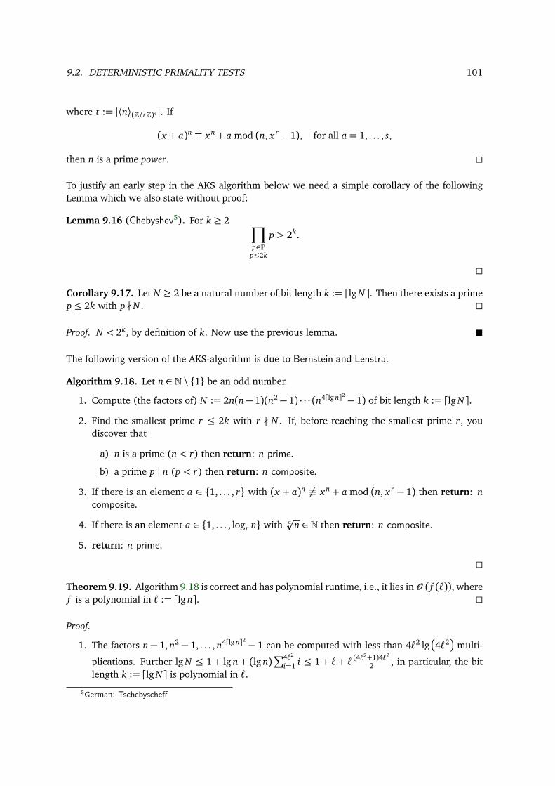
9.2. DETERMINISTIC PRIMALITY TESTS 101
where t := |⟨n⟩(Z/rZ)∗ |. If
(x + a)n ≡ xn + a mod (n, x r − 1), for all a = 1, . . . , s,
then n is a prime power.
To justify an early step in the AKS algorithm below we need a simple corollary of the followingLemma which we also state without proof:
Lemma 9.16 (Chebyshev5). For k ≥ 2 ∏p∈P
p≤2k
p > 2k.
Corollary 9.17. Let N ≥ 2 be a natural number of bit length k := ⌈lg N⌉. Then there exists a primep ≤ 2k with p ∤ N .
Proof. N < 2k, by definition of k. Now use the previous lemma.
The following version of the AKS-algorithm is due to Bernstein and Lenstra.
Algorithm 9.18. Let n ∈ N \ 1 be an odd number.
1. Compute (the factors of) N := 2n(n− 1)(n2 − 1) · · · (n4⌈lg n⌉2 − 1) of bit length k := ⌈lg N⌉.2. Find the smallest prime r ≤ 2k with r ∤ N . If, before reaching the smallest prime r, you
discover that
a) n is a prime (n< r) then return: n prime.
b) a prime p | n (p < r) then return: n composite.
3. If there is an element a ∈ 1, . . . , r with (x + a)n ≡ xn + a mod (n, x r − 1) then return: ncomposite.
4. If there is an element a ∈ 1, . . . , logr n with apn ∈ N then return: n composite.
5. return: n prime.
Theorem 9.19. Algorithm 9.18 is correct and has polynomial runtime, i.e., it lies in O ( f (ℓ)), wheref is a polynomial in ℓ := ⌈lg n⌉.
Proof.
1. The factors n− 1, n2 − 1, . . . , n4⌈lg n⌉2 − 1 can be computed with less than 4ℓ2 lg4ℓ2
multi-
plications. Further lg N ≤ 1+ lg n+ (lg n)∑4ℓ2
i=1 i ≤ 1+ ℓ+ ℓ (4ℓ2+1)4ℓ2
2 , in particular, the bitlength k := ⌈lg N⌉ is polynomial in ℓ.
5German: Tschebyscheff
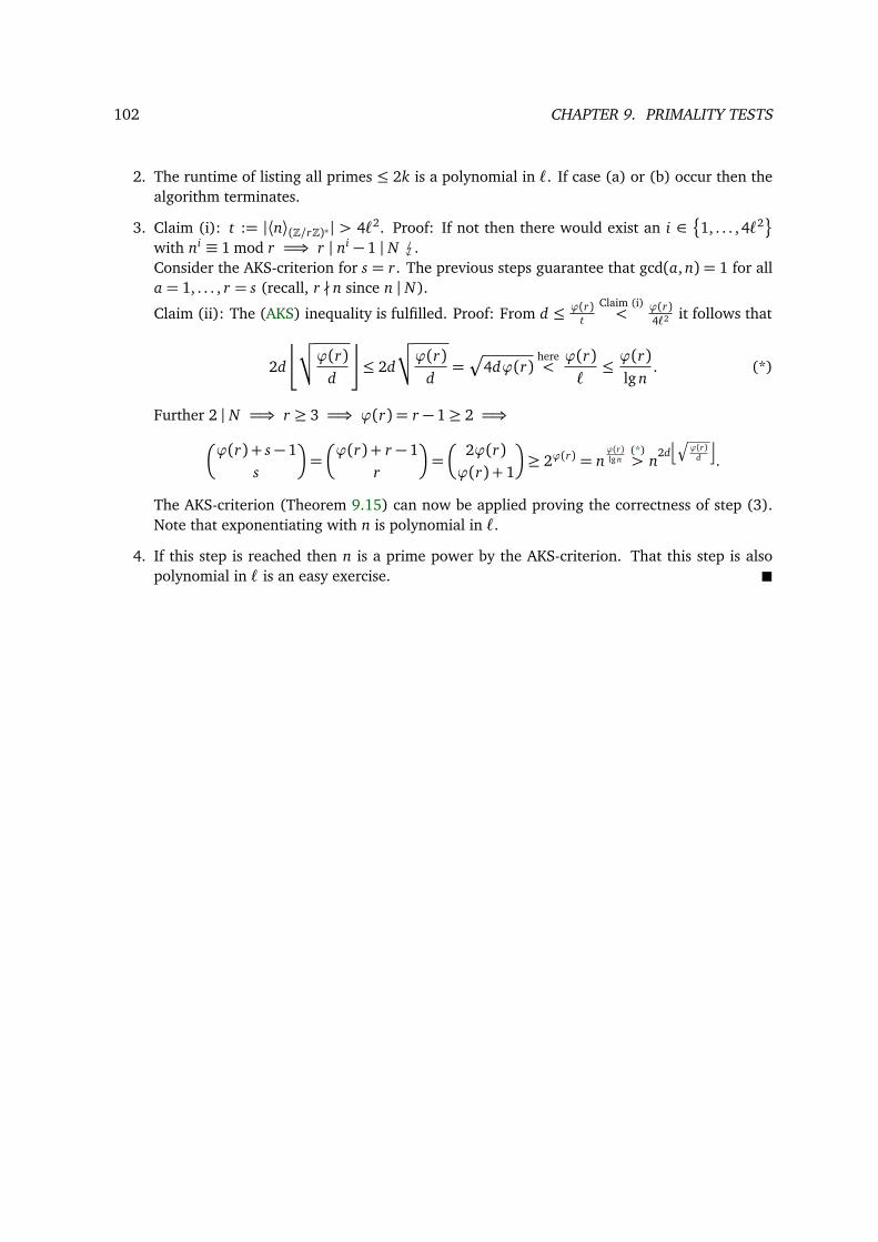
102 CHAPTER 9. PRIMALITY TESTS
2. The runtime of listing all primes ≤ 2k is a polynomial in ℓ. If case (a) or (b) occur then thealgorithm terminates.
3. Claim (i): t := |⟨n⟩(Z/rZ)∗ | > 4ℓ2. Proof: If not then there would exist an i ∈ 1, . . . , 4ℓ2
with ni ≡ 1 mod r =⇒ r | ni − 1 | N .Consider the AKS-criterion for s = r. The previous steps guarantee that gcd(a, n) = 1 for alla = 1, . . . , r = s (recall, r ∤ n since n | N).
Claim (ii): The (AKS) inequality is fulfilled. Proof: From d ≤ φ(r)t
Claim (i)<
φ(r)4ℓ2 it follows that
2d
√√φ(r)d
≤ 2d
√√φ(r)d=Æ
4dφ(r)here<φ(r)ℓ≤ φ(r)
lg n. (*)
Further 2 | N =⇒ r ≥ 3 =⇒ φ(r) = r − 1≥ 2 =⇒φ(r) + s− 1
s
=φ(r) + r − 1
r
=
2φ(r)φ(r) + 1
≥ 2φ(r) = n
φ(r)lg n
(*)> n
2djÇ
φ(r)d
k.
The AKS-criterion (Theorem 9.15) can now be applied proving the correctness of step (3).Note that exponentiating with n is polynomial in ℓ.
4. If this step is reached then n is a prime power by the AKS-criterion. That this step is alsopolynomial in ℓ is an easy exercise.
Chapter 10
Integer Factorization
Recall Remark 8.10: In 2009 the factoring of a number of 768 bits was performed. Still, thefollowing quote from [KAF+10] shows how hard this task was:
The following effort was involved. We spent half a year on 80 processors on polynomialselection. This was about 3% of the main task, the sieving, which was done on manyhundreds of machines and took almost two years. ...
So factorization is still hard, there is until today no polynomial algorithm known.
10.1 Pollard’s p− 1 method
Pollard invented this method in 1974.
Definition 10.1. Let B ∈ N. An n ∈ N is called
1. B-smooth if all its prime divisors are less than or equal to B.
2. B-powersmooth if all its prime power divisors are less than or equal to B.
We now describe Pollard’s p − 1 method to factor a composite integer n ∈ N where p is a primedivisor of n:
1. If gcd(a, n) = 1 for an a ∈ Z then ap−1 ≡ 1 mod p (Fermat’s little theorem).
2. Assume p − 1 is B-powersmooth for a “small” bound B ∈ N. Then p − 1 | lcm1, . . . , B andhence alcm1,...,B ≡ 1 mod p, or equivalently p | alcm1,...,B − 1. In particular:
gcd(alcm1,...,B − 1, n)> 1
and we have found a divisor1 of n.
3. A good heuristic value for B is B ≥ n12(1− 1
e ) ≈ n0.316. So for a fixed B the method should beable to cover all n ≤ B2 e
e−1 ≈ B3.164. Typically one chooses B ≈ 106 which allows handlingnumbers n≤ 1019.
1Of course, the gcd might be n.
103
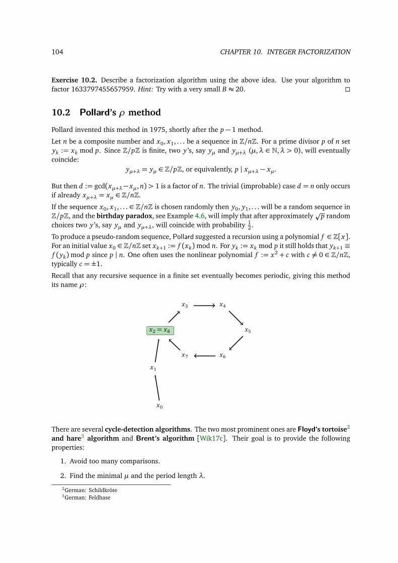
104 CHAPTER 10. INTEGER FACTORIZATION
Exercise 10.2. Describe a factorization algorithm using the above idea. Use your algorithm tofactor 1633797455657959. Hint: Try with a very small B ≈ 20.
10.2 Pollard’s ρ method
Pollard invented this method in 1975, shortly after the p− 1 method.
Let n be a composite number and x0, x1, . . . be a sequence in Z/nZ. For a prime divisor p of n setyk := xk mod p. Since Z/pZ is finite, two y ’s, say yµ and yµ+λ (µ,λ ∈ N,λ > 0), will eventuallycoincide:
yµ+λ = yµ ∈ Z/pZ, or equivalently, p | xµ+λ − xµ.
But then d := gcd(xµ+λ− xµ, n)> 1 is a factor of n. The trivial (improbable) case d = n only occursif already xµ+λ = xµ ∈ Z/nZ.If the sequence x0, x1, . . . ∈ Z/nZ is chosen randomly then y0, y1, . . . will be a random sequence inZ/pZ, and the birthday paradox, see Example 4.6, will imply that after approximately
pp random
choices two y ’s, say yµ and yµ+λ, will coincide with probability 12 .
To produce a pseudo-random sequence, Pollard suggested a recursion using a polynomial f ∈ Z[x].For an initial value x0 ∈ Z/nZ set xk+1 := f (xk)mod n. For yk := xk mod p it still holds that yk+1 ≡f (yk)mod p since p | n. One often uses the nonlinear polynomial f := x2 + c with c = 0 ∈ Z/nZ,typically c = ±1.
Recall that any recursive sequence in a finite set eventually becomes periodic, giving this methodits name ρ:
x0
x1
x2 = x8
x3 x4
x5
x6x7
There are several cycle-detection algorithms. The two most prominent ones are Floyd’s tortoise2
and hare3 algorithm and Brent’s algorithm [Wik17c]. Their goal is to provide the followingproperties:
1. Avoid too many comparisons.
2. Find the minimal µ and the period length λ.
2German: Schildkröte3German: Feldhase
10.3. FERMAT ’S METHOD 105
Of course, only the first goal is relevant for us, where the comparison step in the cycle-detectionalgorithm has to be replaced by the gcd computation: gcd(yµ+λ − yµ, n).
The following version of the Pollard’s ρ method is based on Floyd’s algorithm:
Algorithm 10.3 (Pollard’s ρ method). Given a composite number n ∈ N the following algorithmreturns a nontrivial factor of n or fail.
1. x := 1, z := 1, d := 1
2. while d = 1 do
a) x := f (x)
b) z := f ( f (z))
c) d := gcd(z − x , n)
d) if d = n then return fail
3. return d
The complexity of this method is due to the birthday paradox O pp≤ O n 1
4
.
10.3 Fermat’s method
Fermat’s method for factoring a composite number n tries to write it as the difference of twosquares n = x2 − y2, yielding the factorization n = (x + y)(x − y). Indeed, for a composite oddnumber n = ab such a representation always exists: Setting x := a+b
2 and y := a−b2 we recover
a = x + y and b = x − y .
Example 10.4. Let n = 7429. x = 227 and y = 210 satisfy x2 − y2 = n with x − y = 17 andx + y = 437. Hence n= 17 · 437.
In the following we discuss generalizations of this attempt, also with ideas on how to find x and ywith the needed properties.
10.4 Dixon’s method
Dixon’s method for factoring a composite odd number n is a relaxation of Fermat’s method. It isbased on the following fact: If x , y are integers with
x2 ≡ y2 mod n and x ≡ ±y mod n
then gcd(x − y, n) (and gcd(x + y, n)) is a nontrivial divisor of n.
Example 10.5. Let n= 84923. Taking x = 20712 and y = 16800 we compute x2− y2 = 1728 · n,x − y = 3912 (and x + y = 37512). Hence gcd(x − y, n) = 163 and n= 163 · 521.
Algorithm 10.6 (Dixon’s algorithm). Given a composite number n ∈ N the following algorithmreturns a nontrivial factor of n or fail.
106 CHAPTER 10. INTEGER FACTORIZATION
1. F := p1, . . . , pk ⊂ P be a set of k distinct “small” primes, where k is “small”.4 We call F afactor base5.
2. Find x1, . . . , xm ∈ N (m> k) such that x2i = pe1i
1 · · · pekik mod n.
3. Set vi := ((e1i , . . . , eki)mod 2) ∈ Fk2 for i = 1, . . . , m. Solve the F2-linear system
m∑i=1
ϵi vi = 0 ∈ Fk2.
for the ϵi . If we cannot find a non-trivial solution of this system of equations we need morex i and go back to step (2).
4. Set (a1, . . . , ak) := 12
∑mi=1 ϵi(e1i , . . . , eki) ∈ Zk≥0.6 Define
x :=m∏
i=1
xϵii and y := pa1
1 · · · pakk .
Then
x2 =m∏
i=1
x2ϵii ≡
m∏i=1
pϵi e1i
1 · · · pϵi ekik
= p∑m
i=1 ϵi e1i
1 · · · p∑m
i=1 ϵi eki
k = p2a11 · · · p2ak
k = y2 mod n.
5. If x ≡ y mod n then return gcd(x − y, n) else return fail.
Example 10.7. Again let n= 7429. Take F = 2, 3, 5, 7. We find
x21 = 872 ≡ 22 · 5 · 7 mod 7429
x22 = 882 ≡ 32 · 5 · 7 mod 7429.
Note that in this small example two x i are enough for getting a unique solution to the followingsystem of linear equations.
We havev1 = (2, 0, 1, 1) = (0, 0, 1, 1) = (0, 2, 1, 1) = v2 ∈ F4
2.
Thus ϵ1 = ϵ2 = 1 since 1 · v1 + 1 · v2 = 0 ∈ F42. Hence
(a1, . . . , a4) =12(1 · (2, 0, 1, 1) + 1 · (0, 2, 1, 1)) = (1, 1, 1, 1) ∈ Z4≥0.
Thus, x = 87 ·88≡ 227 mod n and y = 2 ·3 ·5 ·7≡ 210 mod n. As we saw in Example 10.4 abovegcd(x − y, n) = gcd(17, n) = 17.
The complexity of Dixon’s method is O exp2p
2p
log n log log n
.
4Rough heuristic: pk ≈ exp
12
pln n ln ln n.
5German: Faktorbasis6Not over F2 but over Z.
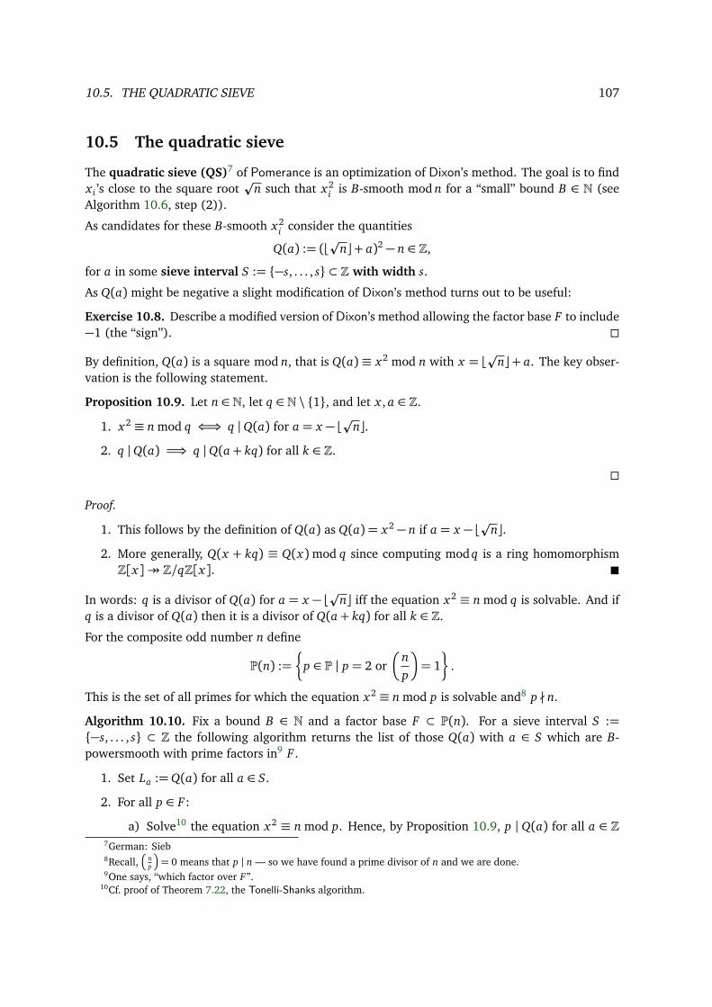
10.5. THE QUADRATIC SIEVE 107
10.5 The quadratic sieve
The quadratic sieve (QS)7 of Pomerance is an optimization of Dixon’s method. The goal is to findx i ’s close to the square root
pn such that x2
i is B-smooth mod n for a “small” bound B ∈ N (seeAlgorithm 10.6, step (2)).
As candidates for these B-smooth x2i consider the quantities
Q(a) := (⌊pn⌋+ a)2 − n ∈ Z,for a in some sieve interval S := −s, . . . , s ⊂ Z with width s.
As Q(a) might be negative a slight modification of Dixon’s method turns out to be useful:
Exercise 10.8. Describe a modified version of Dixon’s method allowing the factor base F to include−1 (the “sign”).
By definition, Q(a) is a square mod n, that is Q(a) ≡ x2 mod n with x = ⌊pn⌋+ a. The key obser-vation is the following statement.
Proposition 10.9. Let n ∈ N, let q ∈ N \ 1, and let x , a ∈ Z.1. x2 ≡ n mod q ⇐⇒ q |Q(a) for a = x − ⌊pn⌋.2. q |Q(a) =⇒ q |Q(a+ kq) for all k ∈ Z.
Proof.
1. This follows by the definition of Q(a) as Q(a) = x2 − n if a = x − ⌊pn⌋.2. More generally, Q(x + kq) ≡ Q(x)mod q since computing modq is a ring homomorphismZ[x]↠Z/qZ[x].
In words: q is a divisor of Q(a) for a = x − ⌊pn⌋ iff the equation x2 ≡ n mod q is solvable. And ifq is a divisor of Q(a) then it is a divisor of Q(a+ kq) for all k ∈ Z.For the composite odd number n define
P(n) :=§
p ∈ P | p = 2 or
np
= 1ª
.
This is the set of all primes for which the equation x2 ≡ n mod p is solvable and8 p ∤ n.
Algorithm 10.10. Fix a bound B ∈ N and a factor base F ⊂ P(n). For a sieve interval S :=−s, . . . , s ⊂ Z the following algorithm returns the list of those Q(a) with a ∈ S which are B-powersmooth with prime factors in9 F .
1. Set La :=Q(a) for all a ∈ S.
2. For all p ∈ F :
a) Solve10 the equation x2 ≡ n mod p. Hence, by Proposition 10.9, p | Q(a) for all a ∈ Z7German: Sieb8Recall,
np
= 0 means that p | n — so we have found a prime divisor of n and we are done.
9One says, “which factor over F”.10Cf. proof of Theorem 7.22, the Tonelli-Shanks algorithm.
108 CHAPTER 10. INTEGER FACTORIZATION
with a ≡ x − ⌊pn⌋mod p.
b) Sieve: For all a ∈ S with a ≡ ±x − ⌊pn⌋mod p, where x is a solution of the equationx2 ≡ n mod p: Replace La by the quotient La
pe , where pe is the maximal power dividingLa which is ≤ B .
3. return the list of those Q(a) with a ∈ S for which La = 1.
The complexity of the Quadratic Sieve is O exp(1+O (1))plog n log log n
.
Remark 10.11. Note that there exists many more general factorization algorithms like the NumberField Sieve. Moreover, there is a wide range of factorization algorithms that are specialized for givensituations. These algorithms are discussed in the lectures Algorithmic and Algebraic Number Theory.See also, for example, [Wik17d] for an overview.
Chapter 11
Elliptic curves
Besides the usual groups modulo a prime number p one can also use other groups for public keycryptosystems like RSA or ElGamal. Clearly, all chosen groups must satisfy that the DLP is hard.One such group of high interest comes from algebraic geometry, in particular, elliptic curves.
11.1 The projective space
We first define the basic structures to work on in algebraic geometry.
Definition 11.1. Let K be a field.
1. The setAn(K) = Kn = (x1, . . . , xn) | x i ∈ K
is called the affine space of dimension n over K . If K is clear from the context then we willsimply write An instead.
2. Two distinct points P,Q ∈ An(K) uniquely determine an (affine) line
PQ := P + K · (Q− P) := P + k(Q− P) | k ∈ K.containing both of them.
3. The projective space of dimension n over K is defined as the set
Pn(K) :=Kn+1 \ 0/K∗ :=
K∗ · x | x ∈ Kn+1 \ 0 .
Again we write Pn if the field K is clear from the context.
4. A point P in Pn(K) can thus be identified with a 1-dimensional subspace of Kn+1. Moregenerally, define the trace of a subset Z ⊂ Pn(K) to be the subset
Z∗ ⊂ Kn+1 =
x ∈ Kn+1 \ 0 | K∗ · x ∈ Z∪ 0.
This gives a one-to-one correspondence between subsets of Pn(K) and those subsets of theunderlying vector space Kn+1 which are unions of 1-dimensional subspaces.
109
110 CHAPTER 11. ELLIPTIC CURVES
Example 11.2. A (projective) line in Pn(K) is the set of all 1-dimensional subspaces of a 2-dimensional subspace L ≤ Kn+1. We identify the projective line with its trace L. Two distinctpoints P,Q ∈ Pn(K) determine a unique projective line PQ := P +Q passing through both of them.P +Q is the 2-dimensional span of P,Q, both viewed as 1-dimensional subspaces of Kn+1.
Homogenous coordinates and affine charts
If x = (x0, . . . , xn) ∈ Kn+1 \ 0 then for the point P = K∗ · x we write
P = (x0 : . . . : xn).
We call x0, . . . , xn ∈ K the homogeneous coordinates of P. They are uniquely determined by Pup to a common nonzero factor:
(x0 : . . . : xn) = (y0 : . . . : yn) ⇐⇒ (y0, . . . , yn) = k · (x0, . . . , xn) for some k ∈ K∗.
Example 11.3. Fix a field K .
1. A1 = a|a ∈ K and P1 = (x : y) | (x , y) ∈ K2 \ 0. Identifying A1 with the affinesubspaces (1, y) | y ∈ K ⊂ K2 or (x , 1) | x ∈ K ⊂ K2 defines two embeddings
φ0 :A1→ P1, y 7→ (1 : y),
φ1 :A1→ P1, x 7→ (x : 1).
These embeddings are also called (standard) affine charts of P1.The elements of the image φ0(A1) ⊂ P1 (resp. φ1(A1) ⊂ P1) are called affine points w.r.t.the chart φ0 (resp. φ1). The point (0 : 1) ∈ P1, corresponding to the y-axis in K2, is the onlynon-affine point w.r.t. φ0. It is called the point at infinity1 w.r.t. φ0. Analogously for (1 : 0)and φ1. Summing up:
P1 = φ0(A1)︸ ︷︷ ︸affine points
∪ (0 : 1)︸ ︷︷ ︸pt at∞
= φ1(A1)︸ ︷︷ ︸affine points
∪ (1 : 0)︸ ︷︷ ︸pt at∞
.
The partial inverses are given by the “projections”
φ−10 :P1 \ (0 : 1) → A1, (x : y) 7→ y
x,
φ−11 :P1 \ (1 : 0) → A1, (x : y) 7→ x
y.
2. A2 = (a, b)|a, b ∈ K and P2 = (x : y : z) | (x , y, z) ∈ K3 \ 0. We have three standardcharts
φ0 :A2→ P2, (y, z) 7→ (1 : y : z),
φ1 :A2→ P2, (x , z) 7→ (x : 1 : z),
φ2 :A2→ P2, (x , y) 7→ (x : y : 1).
1German: unendlich ferner Punkt
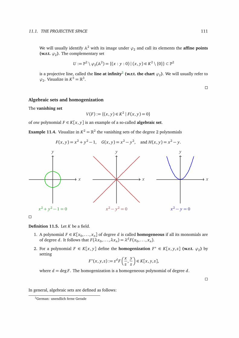
11.1. THE PROJECTIVE SPACE 111
We will usually identify A2 with its image under φ2 and call its elements the affine points(w.r.t. φ2). The complementary set
U := P2 \φ2(A2) = (x : y : 0) | (x , y) ∈ K2 \ 0 ⊂ P2
is a projective line, called the line at infinity2 (w.r.t. the chart φ2). We will usually refer toφ2. Visualize in K3 = R3.
Algebraic sets and homogenization
The vanishing setV (F) := (x , y) ∈ K2 | F(x , y) = 0
of one polynomial F ∈ K[x , y] is an example of a so-called algebraic set.
Example 11.4. Visualize in K2 = R2 the vanishing sets of the degree 2 polynomials
F(x , y) = x2 + y2 − 1, G(x , y) = x2 − y2, and H(x , y) = x2 − y.
x
y
x2 + y2 − 1= 0
x
y
x2 − y2 = 0
x
y
x2 − y = 0
Definition 11.5. Let K be a field.
1. A polynomial F ∈ K[x0, . . . , xn] of degree d is called homogeneous if all its monomials areof degree d. It follows that F(λx0, . . . ,λxn) = λd F(x0, . . . , xn).
2. For a polynomial F ∈ K[x , y] define the homogenization F∗ ∈ K[x , y, z] (w.r.t. φ2) bysetting
F∗(x , y, z) := zd F x
z,
yz
∈ K[x , y, z],
where d = deg F . The homogenization is a homogeneous polynomial of degree d.
In general, algebraic sets are defined as follows:
2German: unendlich ferne Gerade
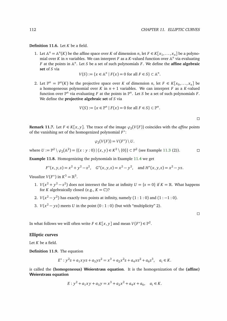
112 CHAPTER 11. ELLIPTIC CURVES
Definition 11.6. Let K be a field.
1. Let An = An(K) be the affine space over K of dimension n, let F ∈ K[x1, . . . , xn] be a polyno-mial over K in n variables. We can interpret F as a K-valued function over An via evaluatingF at the points in An. Let S be a set of such polynomials F . We define the affine algebraicset of S via
V (S) := x ∈ An | F(x) = 0 for all F ∈ S ⊂ An.
2. Let Pn = Pn(K) be the projective space over K of dimension n, let F ∈ K[x0, . . . , xn] bea homogeneous polynomial over K in n + 1 variables. We can interpret F as a K-valuedfunction over Pn via evaluating F at the points in Pn. Let S be a set of such polynomials F .We define the projective algebraic set of S via
V (S) := x ∈ Pn | F(x) = 0 for all F ∈ S ⊂ Pn.
Remark 11.7. Let F ∈ K[x , y]. The trace of the image φ2(V (F)) coincides with the affine pointsof the vanishing set of the homogenized polynomial F∗:
φ2(V (F)) = V (F∗) \ U .
where U := P2 \φ2(A2) = (x : y : 0) | (x , y) ∈ K2 \ 0 ⊂ P2 (see Example 11.3 (2)).
Example 11.8. Homogenizing the polynomials in Example 11.4 we get
F∗(x , y, z) = x2 + y2 − z2, G∗(x , y, z) = x2 − y2, and H∗(x , y, z) = x2 − yz.
Visualize V (F∗) in K3 = R3.
1. V (x2 + y2 − z2) does not intersect the line at infinity U = z = 0 if K = R. What happensfor K algebraically closed (e.g., K = C)?
2. V (x2 − y2) has exactly two points at infinity, namely (1 : 1 : 0) and (1 : −1 : 0).
3. V (x2 − yz) meets U in the point (0 : 1 : 0) (but with “multiplicity” 2).
In what follows we will often write F ∈ K[x , y] and mean V (F∗) ∈ P2.
Elliptic curves
Let K be a field.
Definition 11.9. The equation
E∗ : y2z + a1 x yz + a3 yz2 = x3 + a2 x2z + a4 xz2 + a6z3, ai ∈ K .
is called the (homogeneous) Weierstrass equation. It is the homogenization of the (affine)Weierstrass equation
E : y2 + a1 x y + a3 y = x3 + a2 x2 + a4 x + a6, ai ∈ K .
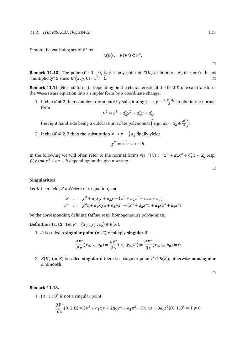
11.1. THE PROJECTIVE SPACE 113
Denote the vanishing set of E∗ byE(K) := V (E∗) ⊂ P2.
Remark 11.10. The point (0 : 1 : 0) is the only point of E(K) at infinity, i.e., at z = 0. It has“multiplicity” 3 since E∗(x , y, 0) : x3 = 0.
Remark 11.11 (Normal forms). Depending on the characteristic of the field K one can transformthe Weierstrass equation into a simpler form by a coordinate change:
1. If char K = 2 then complete the square by substituting y → y − a1 x+a32 to obtain the normal
formy2 = x3 + a′2 x2 + a′4 x + a′6,
the right hand side being a cubical univariate polynomial
e.g., a′2 = a2 +a2
14
.
2. If char K = 2, 3 then the substitution x → x − 13 a′2 finally yields
y2 = x3 + ax + b.
In the following we will often refer to the normal forms via f (x) := x3 + a′2 x2 + a′4 x + a′6 resp.f (x) := x3 + ax + b depending on the given setting.
Singularities
Let K be a field, E a Weierstrass equation, and
F := y2 + a1 x y + a3 y − (x3 + a2 x2 + a4 x + a6),
F∗ := y2z + a1 x yz + a3 yz2 − (x3 + a2 x2z + a4 xz2 + a6z3)
be the corresponding defining (affine resp. homogeneous) polynomials.
Definition 11.12. Let P = (x0 : y0 : z0) ∈ E(K).
1. P is called a singular point (of E) or simply singular if
∂ F∗∂ x(x0, y0, z0) =
∂ F∗∂ y(x0, y0, z0) =
∂ F∗∂ z(x0, y0, z0) = 0.
2. E(K) (or E) is called singular if there is a singular point P ∈ E(K), otherwise nonsingularor smooth.
Remark 11.13.
1. (0 : 1 : 0) is not a singular point:
∂ F∗∂ z(0, 1, 0) = (y2 + a1 x y + 2a3 yz − a2 x2 − 2a4 xz − 3a6z2)(0, 1, 0) = 1 = 0.
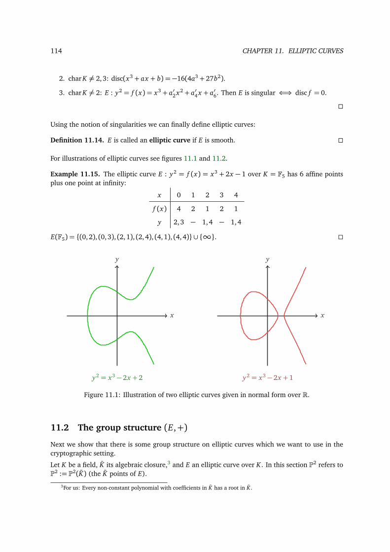
114 CHAPTER 11. ELLIPTIC CURVES
2. char K = 2, 3: disc(x3 + ax + b) = −16(4a3 + 27b2).
3. char K = 2: E : y2 = f (x) = x3 + a′2 x2 + a′4 x + a′6. Then E is singular ⇐⇒ disc f = 0.
Using the notion of singularities we can finally define elliptic curves:
Definition 11.14. E is called an elliptic curve if E is smooth.
For illustrations of elliptic curves see figures 11.1 and 11.2.
Example 11.15. The elliptic curve E : y2 = f (x) = x3 + 2x − 1 over K = F5 has 6 affine pointsplus one point at infinity:
x 0 1 2 3 4
f (x) 4 2 1 2 1
y 2, 3 − 1, 4 − 1, 4
E(F5) = (0, 2), (0, 3), (2, 1), (2, 4), (4, 1), (4, 4) ∪ ∞.
x
y
y2 = x3 − 2x + 2
x
y
y2 = x3 − 2x + 1
Figure 11.1: Illustration of two elliptic curves given in normal form over R.
11.2 The group structure (E,+)
Next we show that there is some group structure on elliptic curves which we want to use in thecryptographic setting.
Let K be a field, K its algebraic closure,3 and E an elliptic curve over K . In this section P2 refers toP2 := P2(K) (the K points of E).
3For us: Every non-constant polynomial with coefficients in K has a root in K .
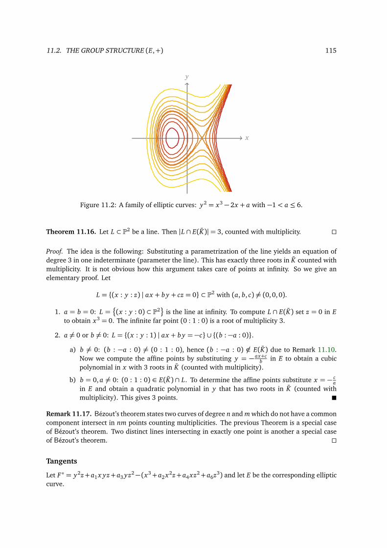
11.2. THE GROUP STRUCTURE (E,+) 115
x
y
Figure 11.2: A family of elliptic curves: y2 = x3 − 2x + a with −1< a ≤ 6.
Theorem 11.16. Let L ⊂ P2 be a line. Then |L ∩ E(K)|= 3, counted with multiplicity.
Proof. The idea is the following: Substituting a parametrization of the line yields an equation ofdegree 3 in one indeterminate (parameter the line). This has exactly three roots in K counted withmultiplicity. It is not obvious how this argument takes care of points at infinity. So we give anelementary proof. Let
L = (x : y : z) | ax + b y + cz = 0 ⊂ P2 with (a, b, c) = (0, 0, 0).
1. a = b = 0: L =(x : y : 0) ⊂ P2
is the line at infinity. To compute L ∩ E(K) set z = 0 in Eto obtain x3 = 0. The infinite far point (0 : 1 : 0) is a root of multiplicity 3.
2. a = 0 or b = 0: L = (x : y : 1) | ax + b y = −c ∪ (b : −a : 0).a) b = 0: (b : −a : 0) = (0 : 1 : 0), hence (b : −a : 0) ∈ E(K) due to Remark 11.10.
Now we compute the affine points by substituting y = − ax+cb in E to obtain a cubic
polynomial in x with 3 roots in K (counted with multiplicity).
b) b = 0, a = 0: (0 : 1 : 0) ∈ E(K) ∩ L. To determine the affine points substitute x = − ca
in E and obtain a quadratic polynomial in y that has two roots in K (counted withmultiplicity). This gives 3 points.
Remark 11.17. Bézout’s theorem states two curves of degree n and m which do not have a commoncomponent intersect in nm points counting multiplicities. The previous Theorem is a special caseof Bézout’s theorem. Two distinct lines intersecting in exactly one point is another a special caseof Bézout’s theorem.
Tangents
Let F∗ = y2z+a1 x yz+a3 yz2− (x3+a2 x2z+a4 xz2+a6z3) and let E be the corresponding ellipticcurve.
116 CHAPTER 11. ELLIPTIC CURVES
Definition 11.18. Let P ∈ E(K). The line
TP :=§(u : v : w) ∈ P2 | ∂ F∗
∂ x(P) · u+ ∂ F∗
∂ y(P) · v + ∂ F∗
∂ z(P) ·w= 0ª
is called the tangent of E at P. One can rewrite the defining equation as ∇F∗(P) · u
vw
= 0,
where ∇= ( ∂∂ x , ∂∂ y , ∂∂ z ).
Remark 11.19.
1. We get the following partial derivations:
∂ F∗∂ x= a1 yz − 3x2 − 2a2 xz − a4z2.
∂ F∗∂ y
= 2yz + a1 xz + a3z2.
∂ F∗∂ z= y2 + a1 x y + 2a3 yz − a2 x2 − 2a4 xz − 3a6z2.
2. If P = (0 : 1 : 0) then ∇F∗(P) = (0, 0, 1). Hence (0 : 1 : 0) ∈ TP = (u : v : w) | w = 0 = U ,the line at infinity.
3. If P = (x : y : 1) then
∂ F∗∂ x(P) = a1 y − 3x2 − 2a2 x − a4.
∂ F∗∂ y(P) = 2y + a1 x + a3.
∂ F∗∂ z(P) = y2 + a1 x y + 2a3 y − a2 x2 − 2a4 x − 3a6.
Verify that ∇F∗(P) · x
y1
= 3F(x , y).
From (2) and (3) we deduce that P ∈ TP for all P ∈ E(K). One can prove that P ∈ E(K) is amultiple intersection point of TP and E(K) with multiplicity at least 2. We have verified this for theinfinite point (0 : 1 : 0) which is an intersection point with multiplicity 3.
Definition 11.20.
1. Fix O := (0 : 1 : 0) ∈ E(K).4
2. For P,Q ∈ E(K) define P ∗Q by E(K)∩ L = P,Q, P ∗Q, where
L :=
PQ if P =QTP if P =Q
.
4O like origin.
11.2. THE GROUP STRUCTURE (E,+) 117
3. Finally define the operation +5 for P,Q ∈ E(K) by
P +Q := (P ∗Q) ∗O.
Lemma 11.21. Let P,Q, R be points on E(K). Then
1. ∗ and + are commutative.
2. (P ∗Q) ∗ P =Q.
3. O ∗O = O.
4. Let L ⊂ P2 be an arbitrary line, E(K)∩ L = P,Q, R, then (P +Q) + R= O.
5. P +O = P.
6. P +Q = O ⇐⇒ P ∗Q = O.
7. + is associative.
8. (E(K),+) is an Abelian group with neutral element O and −P = P ∗O.
9. E(K) is a subgroup of E(K).
Proof.
1. By construction.
2. Definition of ∗ with L = P,Q, P ∗Q.3. Remark 11.19.
4. (P +Q) + R := (((P ∗Q)︸ ︷︷ ︸R
∗O) ∗ R) ∗O(2)= O ∗O
(3)= O.
5. P +O = (P ∗O) ∗O = (O ∗ P) ∗O(2)= P.
6. If P ∗Q = O then P +Q = (P ∗Q) ∗O = O ∗O(2)= O. Now assume P +Q = O. Then
P ∗Q(5)= (P ∗Q) +O = ((P ∗Q) ∗O) ∗O = (P +Q) ∗O = O ∗O
(2)= O.
7. Without a further idea this leads to a lengthy case by case distinction. There exist wonderfulgeometric6 ideas to prove the associativity.
8. Follows from (1), (5), (6) and (7)
9. Let E be defined over K and P,Q ∈ E(K). Then L, L ∩ E is defined over K . Moreover, P ∗Q is,as the third root of L ∩ E(K), also in K . The is a special case of the following simple fact:If f ∈ K[x] with deg f = r and if r − 1 roots are in K then the last root is in K .
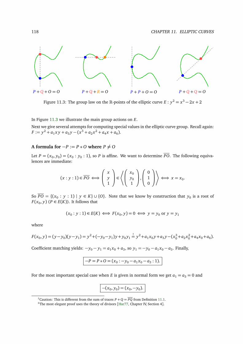
118 CHAPTER 11. ELLIPTIC CURVES
P +Q+O = O P +Q+ R= O P + P +O = O P +Q+Q = O
Figure 11.3: The group law on the R-points of the elliptic curve E : y2 = x3 − 2x + 2
In Figure 11.3 we illustrate the main group actions on E.
Next we give several attempts for computing special values in the elliptic curve group. Recall again:F := y2 + a1 x y + a3 y − (x3 + a2 x2 + a4 x + a6).
A formula for −P := P ∗O where P = O
Let P = (x0, y0) = (x0 : y0 : 1), so P is affine. We want to determine PO. The following equiva-lences are immediate:
(x : y : 1) ∈ PO ⇐⇒ x
y1
∈* x0
y01
, 0
10
+ ⇐⇒ x = x0.
So PO = (x0 : y : 1) | y ∈ K ∪ O. Note that we know by construction that y0 is a root ofF(x0, y) (P ∈ E(K)). It follows that
(x0 : y : 1) ∈ E(K) ⇐⇒ F(x0, y) = 0 ⇐⇒ y = y0 or y = y1
where
F(x0, y) = (y− y0)(y− y1) = y2+(−y0− y1)y+ y0 y1!= y2+a1 x0 y+a3 y−(x3
0+a2 x20+a4 x0+a6).
Coefficient matching yields: −y0 − y1 = a1 x0 + a3, so y1 = −y0 − a1 x0 − a3. Finally,
−P = P ∗O = (x0 : −y0 − a1 x0 − a3 : 1).
For the most important special case when E is given in normal form we get a1 = a3 = 0 and
−(x0, y0) = (x0,−y0).
5Caution: This is different from the sum of traces P +Q = PQ from Definition 11.1.6The most elegant proof uses the theory of divisors [Har77, Chapter IV, Section 4].
11.2. THE GROUP STRUCTURE (E,+) 119
A formula for P ∗Q where P,Q = O
Let P = (x1, y1) = (x1 : y1 : 1) and Q = (x2, y2) = (x2 : y2 : 1) be two affine points. By definition,
P ∗Q = O ⇐⇒ P ∗O =Q ⇐⇒ −P =Q.
Thus, x1 = x2 and y1+ y2+ a1 x1+ a3 = 0. For each line L ⊂ P2 we have: O = (0 : 1 : 0) ∈ L ⇐⇒L ∩A2 is parallel to the y-axis. Let w.l.o.g. P ∗Q = O (otherwise Q = −P). Set
L :=
PQ if P =Q,TP if P =Q.
Then L ∩A2 = (x , y) | y = λx + ν for some λ,ν ∈ K . We have to distinguish two cases:
1. If P =Q then
λ=y2 − y1
x2 − x1and ν= y1 −λx1.
2. If P =Q = (x1, y1) = (x1 : y1 : 1) then
TP ∩A2 =§(x , y) | ∂ F∗
∂ x(P) · x + ∂ F∗
∂ y(P) · y + ∂ F∗
∂ z(P) · 1= 0ª
and
∂ F∗∂ x(P) = a1 y1 − 3x2
1 − 2a2 x1 − a4.
∂ F∗∂ y(P) = 2y1 + a1 x1 + a3.
Solving for y we recover the slope7
λ= −∂ F∗∂ x (P)∂ F∗∂ y (P)
= −a1 y1 − 3x21 − 2a2 x1 − a4
2y1 + a1 x1 + a3.
Further L ∩ E(K) = L ∩A2 ∩ E(K). Again we want F(x ,λx + ν) = 0= −(x − x1)(x − x2)(x − x3).
−(x − x1)(x − x2)(x − x3) = −x3 + (x1 + x2 + x3)x2 + . . .
!= (x +λv)2 + a1 x(x +λv) + a3(x +λv)− (x3 + a2 x2 + a4 x + a6)
= −x3 +λ2 x2 + a1λx2 − a2 x2 + . . .
= −x3 +λ2 + a1λ− a2
x2 + . . .
Coefficient matching at x2 yields: x1 + x2 + x3 = λ2 + a1λ− a2. Finally, P ∗Q = (x3, y3) with
x3 = λ2 + a1λ− a2 − x1 − x2,
y3 = λx3 + ν= λ(x3 − x1) + y1.
7German: Steigung
120 CHAPTER 11. ELLIPTIC CURVES
A formula for P +Q where P,Q = O
We now put together the above computations for P +Q = (P ∗Q) ∗O
P +Q = (λ2 + a1λ− a2 − x1 − x2︸ ︷︷ ︸=x3
,−y1 +λ(x1 − x3)− a1 x1 − a3︸ ︷︷ ︸=y3
).
For the most important special case: y2 = x3 + ax + b, i.e., a1 = a2 = a3 = 0, a4 = a, and a6 = b.Then
λ=y2 − y1
x2 − x1if P =Q or λ=
3x21 + a
2y1if P =Q.
Finally,
x3 = λ2 − x1 − x2,
y3 = −y1 +λ(x1 − x3).
Example 11.22. We take K = F5∼= Z/5Z and y2 = x3 + 2x − 1. Verify that
E(F5) = (0, 2), (0, 3), (2, 1), (2, 4), (4, 1), (4, 4) ∪ O.1. P = (0, 2) =⇒ −P = (0,−2) = (0, 3).
2. Q = (2, 1) =⇒ P +Q = (2, 4).
3. P + P = 2P = (4, 1).
4. (0, 3) + (2, 1) = (4, 1).
Remark 11.23. The choice of O := (0 : 1 : 0) was arbitrary but convenient for two reasons:
1. It is the unique non-affine point w.r.t. the fixed coordinate system.
2. It satisfies O ∗O = O.
11.3 Elliptic curves over finite fields
In order to use the group structure on elliptic curves in the cryptographical setting, we have toinvestigate operations on E over finite fields.
Squares in finite fields
Finding square roots in the finite field Fq is the first step to find Fq-points (i.e., points in E(Fq)) onan elliptic curve E.
Remark 11.24. Let p be a prime and q a power of p. Furthermore, recall the squaring homomor-phism qn : (Z/nZ)∗→ (Z/nZ)∗, x 7→ x2 mod n from Remark 7.5. Now let k := |F∗q|.
11.3. ELLIPTIC CURVES OVER FINITE FIELDS 121
1. ker qk = ±1. Hence
|(F∗q)2|= q−1
2 for q odd,q− 1 for q even.
2. Define for q odd the quadratic character
χ : F∗q→ ±1 ⊂ F∗q, x 7→ xq−1
2 .
Note that χ(a) = 1 ⇐⇒ a ∈ (F∗q)2. This follows easily from (1) generalizing Theorem 7.8by Euler.
Algorithm 11.25. Given an odd prime power q and an a ∈ F∗q with χ(a) = 1. Return b ∈ F∗q with
b2 = a using the Tonelli-Shanks algorithm from the proof of Theorem 7.22, slightly generalized forprime powers.
Counting points
Let E be an elliptic curve over Fq and N := |E(Fq)|.Theorem 11.26 (Hasse-Weil). Let a := q+1−N and α,β be the roots of the quadratic polynomialx2 − ax + q. Then
|a| ≤ 2p
q.
Further,
|E(Fqm)|= qm + 1− (αm + βm)
for all m ∈ N.
Proof. A good reference is [Was08, Theorem 4.2].
Remark 11.27. For N = |E(Fq)| the Hasse-Weil theorem estimates
q+ 1− 2p
q ≤ N ≤ q+ 1+ 2p
q.
If q is a prime one can show that each natural number in this interval occurs as the order of anelliptic curve E(Fq).
Example 11.28. Let E : y2 = x3+7x+1 be an elliptic curve of F101. It is possible to show that thepoint (0, 1) ∈ E(F101) has order 116 (see Algorithm 11.31 below), so N = |E(F101)| is a multipleof 116. But the Hasse-Weil theorem says that
81≤ 101+ 1− 2p
101≤ N ≤ 101+ 1+ 2p
101≤ 123,
and the only multiple of 116 in this range is 116. Hence, E(F101) is cyclic of order N := |E(F101)|=116, generated by the point (0, 1).
122 CHAPTER 11. ELLIPTIC CURVES
Example 11.29. With little effort we can determine all the points of E : y2+ x y = x3+1 over thesmall field F2:
E(F2) = O, (0, 1), (1, 0), (1, 1).So N = |E(F2)| = 4. We can thus compute a := q + 1− N = −1 where q = 2. If we now go into afield extension, say F2101 we can use the Hasse-Weil theorem to count the number of points: Firstwe compute the roots α,β of x2 − (−1)x + 2 which are −1±p−7
2 . Then we apply the formula fromabove:
|E(F2101)| = 2101 + 1−−1+
p−72
101
+
−1−p−72
101= 2101 + 1− 2969292210605269
= 2535301200456455833701195805484≈ 2.5 · 1030.
Theorem 11.30 ([Was08, Theorem 4.3]). Let p be a prime and q = pn and define N := q+ 1− afor some a ∈ Z with |a| ≤ 2
pq. Then there is an elliptic curve E defined over Fq with |E(Fq)| = N
if and only if a satisfies one of the following conditions:
1. gcd(a, p) = 1.
2. n is even and a = ±2p
q.
3. n is even, p ≡ 1 mod 3, and a = ±pq.
4. n is odd, p = 2 or p = 3, and a = ±pn+1
2 .
5. n is even, p ≡ 1 mod 4, and a = 0.
6. n is odd and a = 0.
Let P ∈ E(Fq). We want to find the order of P as an element of the group E(Fq). We know thatN P = O. Of course we don’t know N yet, but we know that q+ 1− 2
pq ≤ N ≤ q+ 1+ 2
pq. One
could of course try all values in this interval. This would take 4p
q steps. The following algorithmis faster and runs in about 4q
14 steps:
Algorithm 11.31 (Baby step, giant step, [Was08, § 4.3.4]). Given P ∈ E(Fq) compute its order.
1. Compute Q = (q+ 1)P.
2. Choose an integer m> q14 . Compute and save the points jP for j = 0, . . . , m (baby steps).
3. Compute the points
Q+ k(2mP) for k = −m, . . . , m (giant steps)
until Q+ k(2mP) = ± jP. Then M P = O with M := q+ 1+ 2mk∓ j.
4. Factor M = pe11 · · · per
r . Compute (M/pi)P for i = 1, . . . , r. If (M/pi)P = O for some i, replaceM with M/pi and repeat the step until (M/pi)P = O for all i. Then M is the order of P.
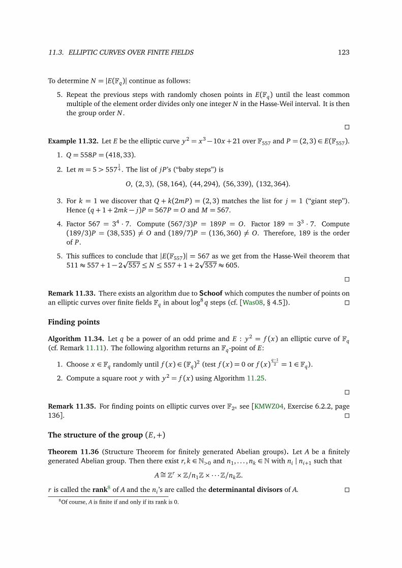
11.3. ELLIPTIC CURVES OVER FINITE FIELDS 123
To determine N = |E(Fq)| continue as follows:
5. Repeat the previous steps with randomly chosen points in E(Fq) until the least commonmultiple of the element order divides only one integer N in the Hasse-Weil interval. It is thenthe group order N .
Example 11.32. Let E be the elliptic curve y2 = x3−10x +21 over F557 and P = (2, 3) ∈ E(F557).
1. Q = 558P = (418, 33).
2. Let m= 5> 55714 . The list of jP ’s (“baby steps”) is
O, (2, 3), (58, 164), (44, 294), (56, 339), (132, 364).
3. For k = 1 we discover that Q + k(2mP) = (2, 3) matches the list for j = 1 (“giant step”).Hence (q+ 1+ 2mk− j)P = 567P = O and M = 567.
4. Factor 567 = 34 · 7. Compute (567/3)P = 189P = O. Factor 189 = 33 · 7. Compute(189/3)P = (38, 535) = O and (189/7)P = (136, 360) = O. Therefore, 189 is the orderof P.
5. This suffices to conclude that |E(F557)| = 567 as we get from the Hasse-Weil theorem that511≈ 557+ 1− 2
p557≤ N ≤ 557+ 1+ 2
p557≈ 605.
Remark 11.33. There exists an algorithm due to Schoof which computes the number of points onan elliptic curves over finite fields Fq in about log8 q steps (cf. [Was08, § 4.5]).
Finding points
Algorithm 11.34. Let q be a power of an odd prime and E : y2 = f (x) an elliptic curve of Fq(cf. Remark 11.11). The following algorithm returns an Fq-point of E:
1. Choose x ∈ Fq randomly until f (x) ∈ (Fq)2 (test f (x) = 0 or f (x)q−1
2 = 1 ∈ Fq).
2. Compute a square root y with y2 = f (x) using Algorithm 11.25.
Remark 11.35. For finding points on elliptic curves over F2n see [KMWZ04, Exercise 6.2.2, page136].
The structure of the group (E,+)
Theorem 11.36 (Structure Theorem for finitely generated Abelian groups). Let A be a finitelygenerated Abelian group. Then there exist r, k ∈ N>0 and n1, . . . , nk ∈ N with ni | ni+1 such that
A∼= Zr ×Z/n1Z× · · ·Z/nkZ.
r is called the rank8 of A and the ni ’s are called the determinantal divisors of A. 8Of course, A is finite if and only if its rank is 0.
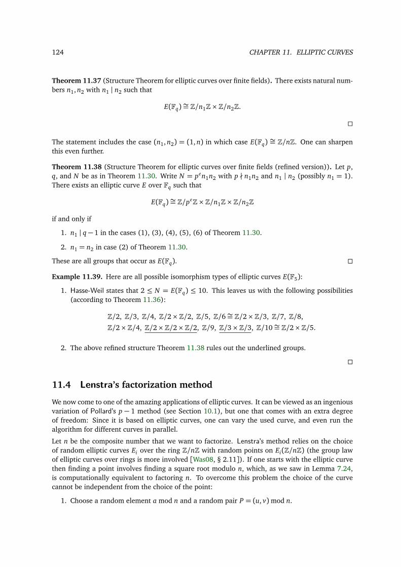
124 CHAPTER 11. ELLIPTIC CURVES
Theorem 11.37 (Structure Theorem for elliptic curves over finite fields). There exists natural num-bers n1, n2 with n1 | n2 such that
E(Fq)∼= Z/n1Z×Z/n2Z.
The statement includes the case (n1, n2) = (1, n) in which case E(Fq) ∼= Z/nZ. One can sharpenthis even further.
Theorem 11.38 (Structure Theorem for elliptic curves over finite fields (refined version)). Let p,q, and N be as in Theorem 11.30. Write N = pen1n2 with p ∤ n1n2 and n1 | n2 (possibly n1 = 1).There exists an elliptic curve E over Fq such that
E(Fq)∼= Z/peZ×Z/n1Z×Z/n2Z
if and only if
1. n1 | q− 1 in the cases (1), (3), (4), (5), (6) of Theorem 11.30.
2. n1 = n2 in case (2) of Theorem 11.30.
These are all groups that occur as E(Fq).
Example 11.39. Here are all possible isomorphism types of elliptic curves E(F5):
1. Hasse-Weil states that 2 ≤ N = E(Fq) ≤ 10. This leaves us with the following possibilities(according to Theorem 11.36):
Z/2, Z/3, Z/4, Z/2×Z/2, Z/5, Z/6∼= Z/2×Z/3, Z/7, Z/8,
Z/2×Z/4, Z/2×Z/2×Z/2, Z/9, Z/3×Z/3, Z/10∼= Z/2×Z/5.
2. The above refined structure Theorem 11.38 rules out the underlined groups.
11.4 Lenstra’s factorization method
We now come to one of the amazing applications of elliptic curves. It can be viewed as an ingeniousvariation of Pollard’s p − 1 method (see Section 10.1), but one that comes with an extra degreeof freedom: Since it is based on elliptic curves, one can vary the used curve, and even run thealgorithm for different curves in parallel.
Let n be the composite number that we want to factorize. Lenstra’s method relies on the choiceof random elliptic curves Ei over the ring Z/nZ with random points on Ei(Z/nZ) (the group lawof elliptic curves over rings is more involved [Was08, § 2.11]). If one starts with the elliptic curvethen finding a point involves finding a square root modulo n, which, as we saw in Lemma 7.24,is computationally equivalent to factoring n. To overcome this problem the choice of the curvecannot be independent from the choice of the point:
1. Choose a random element a mod n and a random pair P = (u, v)mod n.
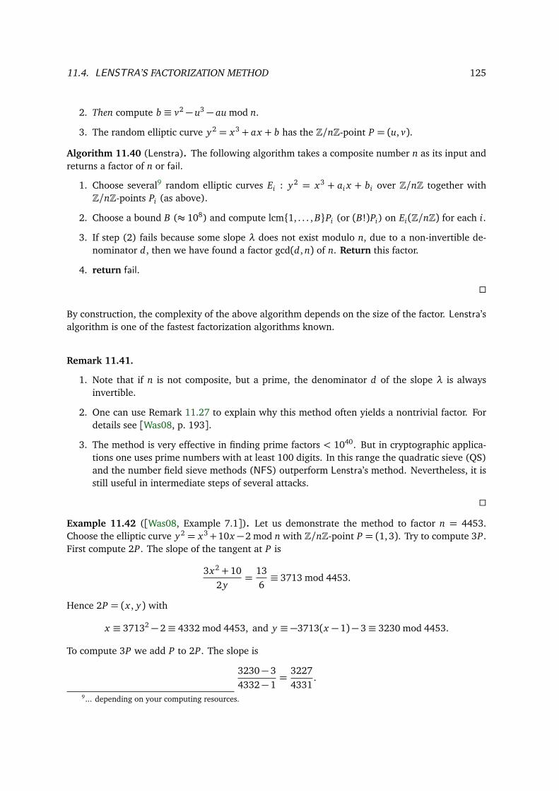
11.4. LENSTRA’S FACTORIZATION METHOD 125
2. Then compute b ≡ v2 − u3 − au mod n.
3. The random elliptic curve y2 = x3 + ax + b has the Z/nZ-point P = (u, v).
Algorithm 11.40 (Lenstra). The following algorithm takes a composite number n as its input andreturns a factor of n or fail.
1. Choose several9 random elliptic curves Ei : y2 = x3 + ai x + bi over Z/nZ together withZ/nZ-points Pi (as above).
2. Choose a bound B (≈ 108) and compute lcm1, . . . , BPi (or (B!)Pi) on Ei(Z/nZ) for each i.
3. If step (2) fails because some slope λ does not exist modulo n, due to a non-invertible de-nominator d, then we have found a factor gcd(d, n) of n. Return this factor.
4. return fail.
By construction, the complexity of the above algorithm depends on the size of the factor. Lenstra’salgorithm is one of the fastest factorization algorithms known.
Remark 11.41.
1. Note that if n is not composite, but a prime, the denominator d of the slope λ is alwaysinvertible.
2. One can use Remark 11.27 to explain why this method often yields a nontrivial factor. Fordetails see [Was08, p. 193].
3. The method is very effective in finding prime factors < 1040. But in cryptographic applica-tions one uses prime numbers with at least 100 digits. In this range the quadratic sieve (QS)and the number field sieve methods (NFS) outperform Lenstra’s method. Nevertheless, it isstill useful in intermediate steps of several attacks.
Example 11.42 ([Was08, Example 7.1]). Let us demonstrate the method to factor n = 4453.Choose the elliptic curve y2 = x3+10x −2 mod n with Z/nZ-point P = (1, 3). Try to compute 3P.First compute 2P. The slope of the tangent at P is
3x2 + 102y
=136≡ 3713 mod 4453.
Hence 2P = (x , y) with
x ≡ 37132 − 2≡ 4332 mod 4453, and y ≡ −3713(x − 1)− 3≡ 3230 mod 4453.
To compute 3P we add P to 2P. The slope is
3230− 34332− 1
=32274331
.
9... depending on your computing resources.
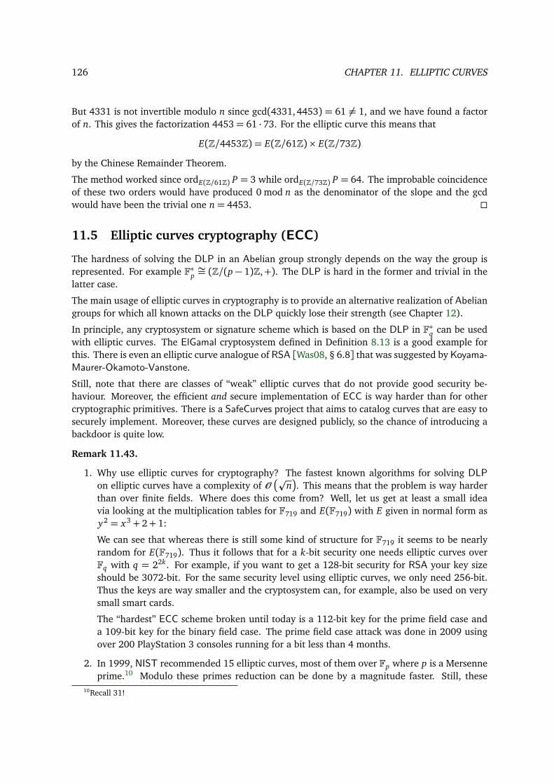
126 CHAPTER 11. ELLIPTIC CURVES
But 4331 is not invertible modulo n since gcd(4331, 4453) = 61 = 1, and we have found a factorof n. This gives the factorization 4453= 61 · 73. For the elliptic curve this means that
E(Z/4453Z) = E(Z/61Z)× E(Z/73Z)
by the Chinese Remainder Theorem.
The method worked since ordE(Z/61Z) P = 3 while ordE(Z/73Z) P = 64. The improbable coincidenceof these two orders would have produced 0 mod n as the denominator of the slope and the gcdwould have been the trivial one n= 4453.
11.5 Elliptic curves cryptography (ECC)
The hardness of solving the DLP in an Abelian group strongly depends on the way the group isrepresented. For example F∗p ∼= (Z/(p − 1)Z,+). The DLP is hard in the former and trivial in thelatter case.
The main usage of elliptic curves in cryptography is to provide an alternative realization of Abeliangroups for which all known attacks on the DLP quickly lose their strength (see Chapter 12).
In principle, any cryptosystem or signature scheme which is based on the DLP in F∗q can be usedwith elliptic curves. The ElGamal cryptosystem defined in Definition 8.13 is a good example forthis. There is even an elliptic curve analogue of RSA [Was08, § 6.8] that was suggested by Koyama-Maurer-Okamoto-Vanstone.
Still, note that there are classes of “weak” elliptic curves that do not provide good security be-haviour. Moreover, the efficient and secure implementation of ECC is way harder than for othercryptographic primitives. There is a SafeCurves project that aims to catalog curves that are easy tosecurely implement. Moreover, these curves are designed publicly, so the chance of introducing abackdoor is quite low.
Remark 11.43.
1. Why use elliptic curves for cryptography? The fastest known algorithms for solving DLPon elliptic curves have a complexity of O pn
. This means that the problem is way harder
than over finite fields. Where does this come from? Well, let us get at least a small ideavia looking at the multiplication tables for F719 and E(F719) with E given in normal form asy2 = x3 + 2+ 1:
We can see that whereas there is still some kind of structure for F719 it seems to be nearlyrandom for E(F719). Thus it follows that for a k-bit security one needs elliptic curves overFq with q = 22k. For example, if you want to get a 128-bit security for RSA your key sizeshould be 3072-bit. For the same security level using elliptic curves, we only need 256-bit.Thus the keys are way smaller and the cryptosystem can, for example, also be used on verysmall smart cards.
The “hardest” ECC scheme broken until today is a 112-bit key for the prime field case anda 109-bit key for the binary field case. The prime field case attack was done in 2009 usingover 200 PlayStation 3 consoles running for a bit less than 4 months.
2. In 1999, NIST recommended 15 elliptic curves, most of them over Fp where p is a Mersenneprime.10 Modulo these primes reduction can be done by a magnitude faster. Still, these
10Recall 31!
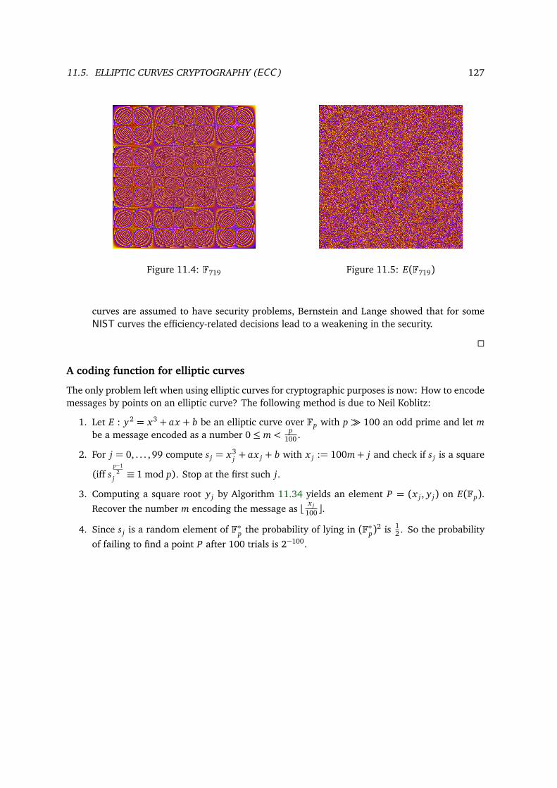
11.5. ELLIPTIC CURVES CRYPTOGRAPHY (ECC) 127
Figure 11.4: F719 Figure 11.5: E(F719)
curves are assumed to have security problems, Bernstein and Lange showed that for someNIST curves the efficiency-related decisions lead to a weakening in the security.
A coding function for elliptic curves
The only problem left when using elliptic curves for cryptographic purposes is now: How to encodemessages by points on an elliptic curve? The following method is due to Neil Koblitz:
1. Let E : y2 = x3 + ax + b be an elliptic curve over Fp with p≫ 100 an odd prime and let mbe a message encoded as a number 0≤ m< p
100 .
2. For j = 0, . . . , 99 compute s j = x3j + ax j + b with x j := 100m+ j and check if s j is a square
(iff sp−1
2j ≡ 1 mod p). Stop at the first such j.
3. Computing a square root y j by Algorithm 11.34 yields an element P = (x j , y j) on E(Fp).Recover the number m encoding the message as ⌊ x j
100⌋.4. Since s j is a random element of F∗p the probability of lying in (F∗p)2 is 1
2 . So the probability
of failing to find a point P after 100 trials is 2−100.
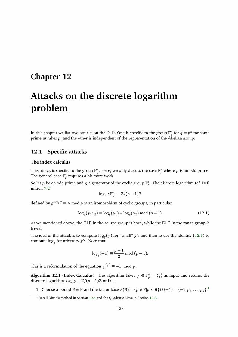
Chapter 12
Attacks on the discrete logarithmproblem
In this chapter we list two attacks on the DLP. One is specific to the group F∗q for q = pn for someprime number p, and the other is independent of the representation of the Abelian group.
12.1 Specific attacks
The index calculus
This attack is specific to the group F∗q. Here, we only discuss the case F∗p where p is an odd prime.The general case F∗q requires a bit more work.
So let p be an odd prime and g a generator of the cyclic group F∗p. The discrete logarithm (cf. Def-inition 7.2)
logg : F∗p→ Z/(p− 1)Z
defined by g logg y ≡ y mod p is an isomorphism of cyclic groups, in particular,
logg(y1 y2)≡ logg(y1) + logg(y2)mod (p− 1). (12.1)
As we mentioned above, the DLP in the source group is hard, while the DLP in the range group istrivial.
The idea of the attack is to compute logg(y) for “small” y ’s and then to use the identity (12.1) tocompute logg for arbitrary y ’s. Note that
logg(−1)≡ p− 12
mod (p− 1).
This is a reformulation of the equation gp−1
2 ≡ −1 mod p.
Algorithm 12.1 (Index Calculus). The algorithm takes y ∈ F∗p = ⟨g⟩ as input and returns thediscrete logarithm logg y ∈ Z/(p− 1)Z or fail.
1. Choose a bound B ∈ N and the factor base F(B) = p ∈ P|p ≤ B ∪ −1= −1, p1, . . . , pk.11Recall Dixon’s method in Section 10.4 and the Quadratic Sieve in Section 10.5.
128
12.1. SPECIFIC ATTACKS 129
2. Search for yi ’s for which the lift bi ∈ Z of g yi ∈ F∗p can be factored over F(B), i.e., bi ≡(−1)ei0∏k
j=1 pei j
j mod p. Do this until the set of equations
yi ≡ logg ((−1)ei0)︸ ︷︷ ︸≡0 or p−1
2
+ei1 logg p1 + · · ·+ eik logg pk mod (p− 1)
can be solved for the vector of k unknowns (logg p1, . . . , logg pk). If the search fails returnfail.
3. Search for an ℓ for which the lift b ∈ Z of gℓ · y ∈ F∗p can be factored over F(B), i.e., b ≡(−1)a0∏k
j=1 pa j
j mod p. If the search fails return fail.
4. Solve the equation
ℓ+ logg y ≡ logg ((−1)a0)︸ ︷︷ ︸≡0 or p−1
2
+a1 logg p1 + · · ·+ ak logg pk mod (p− 1)
and return logg y .
Example 12.2 ([Was08, Example 5.1]). We will demonstrate the method by computing the discretelogarithm log3 37 mod 1217, so g = 3, y = 37 and p = 1217. Choosing B = 13 gives the factorbase F(B) = −1, 2, 3, 5, 7, 11, 13. We compute
31 ≡ 31 mod1217324 ≡ (−1)1 ·22 ·7 ·13 mod1217325 ≡ 53 mod1217330 ≡ (−1)1 ·21 ·52 mod1217354 ≡ (−1)1 ·51 ·11 mod1217387 ≡ 13 mod1217
Recall p− 1= 1216. This yields in particular:
log3 2 ≡ 216 mod1216,log3 7 ≡ 113 mod1216,
log3 11 ≡ 1059 mod1216.
Finally, for ℓ= 16, we get 316 · 37≡ 23 · 7 · 11 mod 1217. Therefore,
log3 37≡ 3 log3 2+ log3 7+ log3 11− 16≡ 588 mod 1216.
Remark 12.3. Several remarks on the usage of index calculus and further optimizations:
1. The method was successfully used to compute discrete logarithms modulo a 120-digit prime.
2. Finding the appropriate yi ’s and the ℓ can be done using a version of the quadratic sieve (QS)or the number field sieve (NFS) as in Section 10.5.
130 CHAPTER 12. ATTACKS ON THE DISCRETE LOGARITHM PROBLEM
3. In contrast to F∗p = (Z/pZ)∗, elements of E(Fp) are rarely reductions of elements in E(Z) (orE(Q)). It is thus widely believed that the index calculus cannot be adapted to solve the DLPfor elliptic curves.
12.2 General attacks
By general attacks we mean attacks applicable for all representations of a finite Abelian group.Pollard’s ρ method, cf. Section 10.2, can be modified to give a general probabilistic algorithm tosolve the DLP [Was08, § 5.2.2]. From the many known general attacks on the DLP we only treata modified version of the baby-step-giant-step algorithm.
Baby Step, Giant Step
Let G be an additively written Abelian group with (known) order N . W.l.o.g. we can assume thatG = ⟨P⟩.2
Algorithm 12.4 (Shanks). The following deterministic algorithm takes as input an element Q ∈ Gand returns the discrete logarithm k := logP Q, i.e., the minimal k ∈ N with kP =Q.
1. Fix an m>p
N and compute mP.
2. Compute and save the list L := (iP | 0≤ i < m) (“baby steps”).
3. For j = 0, . . . , m−1 compute the points Q− jmP (“giant steps”) until one matches an elementin L, say iP =Q− jmP.
4. Since Q = kP with k ≡ i + jm mod N return (the smallest such) k.
Proof of correctness. Since m2 > N it follows that 0≤ k < m2. Write k = i+ jm with 0≤ i < m and0≤ j = k−i
m < m. Then Q− jmP = kP − jmP = iP.
Example 12.5 ([Was08, Example 5.2]). Let G = E(F41), where E : y2 = x3+2x+1. Let P = (0, 1)and Q = (30, 40). The group order N is at most 54 by Hasse-Weil, cf. Theorem 11.26, so set m= 8.The list of baby steps iP for 0≤ i < 8 consists of the points
O, (0, 1), (1, 39), (8, 23), (38, 38), (23, 23), (20, 28), (26, 9).
We start calculating the giant steps for j = 0, 1, 2, . . .
(30, 40), (9, 25), (26, 9), . . .
and stop since (26, 9) matches 7P in the list. With i = 7 and j = 2 we compute the discretelogarithm k = 7+ 2 · 8= 23. Indeed: Q = 23P.
2We switched notation a bit for the following example applying the algorithm to elliptic curves.
12.2. GENERAL ATTACKS 131
Remark 12.6. The complexity of this attack can be estimated in the following way: We haveO pN
computations of the points due to the birthday paradoxon. Now we can assume a hashtable to look up if two points match which can be done in O (1). Thus we get a complexity ofO pN
which is much better than general brute force attacks with O (N). Still, for bigger groupsthe algorithm is not practical.
Chapter 13
Digital signatures
For a digital signature or digital signature scheme (DSS) we understand a mathematical schemefor ensuring the authenticity of data. A digital signature should lose its validity if anything in thesigned data was altered. This is one of the major advantages compared to ink on paper signatures.
13.1 Basic Definitions & Notations
Definition 13.1. An asymmetric signature is a 5-tuple (P ,C ,κ : K ′ → K ,S ,V ) with the fol-lowing properties:
1. P is called the set of messages.
2. C is called the set of signatures.
3. κ :K ′→K , d 7→ e is a bijective map from the set of secret signing keys to the set of publicverification keys.
4. S = (Sd :P C )d∈K ′ is a family of multi-valued polynomial algorithms, called the signingalgorithm.
5. V = (Ve : P ×C → 0, 1)e∈K is a family of polynomial algorithms, called the signatureverifications satisfying Vκ(d)(m,Sd(m)) = 1 for all m ∈ P .
Usually, one signs only hash values of messages for performance reasons: “hash-then-sign”. Wewill come to hash functions below.
Definition 13.2. We list the following attack models on a DSS:
1. Key-only attack: The attacker only knows the public verification key of the signer.
2. Known-message attack (KMA): The attacker receives some messages (he did not choosethem) and their corresponding signatures.
3. (Adaptive) chosen-message attack (CMA): The attacker is allowed to (adaptively) choosemessages and receives the corresponding signatures.
132
13.2. SIGNATURES USING OWF WITH TRAPDOORS 133
Definition 13.3. We list the following goals of an attack on a DSS:
1. Total break: Recover the signing key.
2. Universal forgery:1 Forge signatures of any message.
3. Existential forgery: Forge a signature for some message (without the ability to do this forany message).
The strongest security model among the above combinations is the security against universal forgeryunder an adaptive chosen message attack.
13.2 Signatures using OWF with trapdoors
Let f := ( fi)i∈I : X → X be a OWF with trapdoor information (t i)i∈I as in Definition 7.28 (e.g., theRabin function, cf. Example 7.29 or the RSA function, cf. Example 8.2). Set
1. P =C = X ,
2. K = I , K ′ = (i, t i) | i ∈ I, κ : d := (i, t i) 7→ e := i,
3. Sd :P →C , m 7→ f −1e (m) (using the trapdoor information),
4. Ve :P ×C → 0, 1, (m, s) 7→
1 if fe(s) = m0 if fe(s) = m
.
Remark 13.4.
1. Existential forgery is always possible: First choose the signature s, then choose the messagem := fe(s).
2. If the OWF f is multiplicative (e.g., the RSA function: (x y)e = x e y e) then the universalforgery under an adaptive chosen-message attack is possible: To sign m decompose it asm = m1m2 with m1 = m = m2. Ask for the signatures of si of mi (this is allowed in CMAsince mi = m). Compute (m, s) = (m, s1s2) by the multiplicativity of f .
3. Another obvious drawback of this scheme is that the signature has the same length as themessage.
We now give a variant of asymmetric signatures that, under certain assumptions, avoids the abovementioned drawbacks. Recall similar techniques we applied to asymmetric crypto systems in Sec-tion 8.4.
Definition 13.5 (Hash-then-sign). This is a variant of Definition 13.1 with the following modifica-tions (we are still using the notation of this section):
1. P = 0, 1•, C = X .
1German: Fälschung
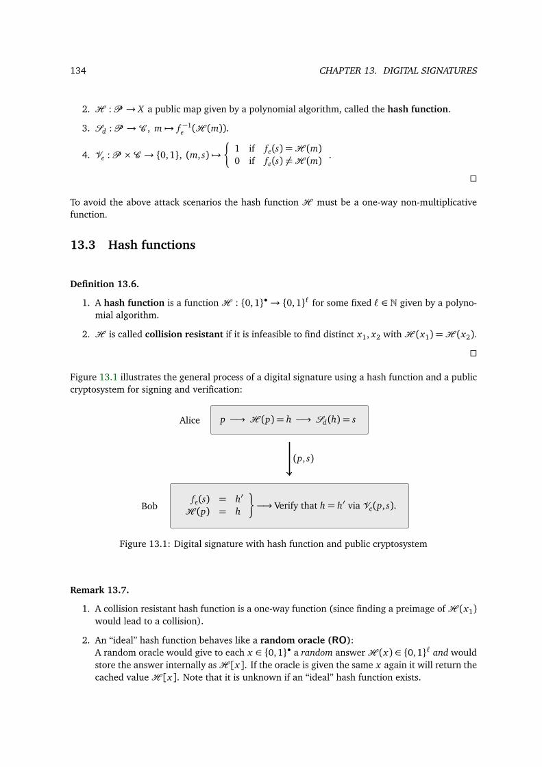
134 CHAPTER 13. DIGITAL SIGNATURES
2. H :P → X a public map given by a polynomial algorithm, called the hash function.
3. Sd :P →C , m 7→ f −1e (H (m)).
4. Ve :P ×C → 0, 1, (m, s) 7→
1 if fe(s) =H (m)0 if fe(s) =H (m) .
To avoid the above attack scenarios the hash function H must be a one-way non-multiplicativefunction.
13.3 Hash functions
Definition 13.6.
1. A hash function is a function H : 0, 1•→ 0, 1ℓ for some fixed ℓ ∈ N given by a polyno-mial algorithm.
2. H is called collision resistant if it is infeasible to find distinct x1, x2 withH (x1) =H (x2).
Figure 13.1 illustrates the general process of a digital signature using a hash function and a publiccryptosystem for signing and verification:
p −→ H (p) = h −→ Sd(h) = sAlice
fe(s) = h′H (p) = h
−→ Verify that h= h′ via Ve(p, s).Bob
(p, s)
Figure 13.1: Digital signature with hash function and public cryptosystem
Remark 13.7.
1. A collision resistant hash function is a one-way function (since finding a preimage ofH (x1)would lead to a collision).
2. An “ideal” hash function behaves like a random oracle (RO):A random oracle would give to each x ∈ 0, 1• a random answerH (x) ∈ 0, 1ℓ and wouldstore the answer internally asH [x]. If the oracle is given the same x again it will return thecached valueH [x]. Note that it is unknown if an “ideal” hash function exists.
13.4. SIGNATURES USING OWF WITHOUT TRAPDOORS 135
3. Note that recently a team of cryptographers found a collision in the SHA-12 hash algo-rithm [Wik17h]. In 2010 the U.S. NIST advised all U.S. federal agencies to no longer useSHA-1 but switch to SHA-2. Still, SHA-1 is used in non-cryptographical applications, for ex-ample, the version control systems GIT or Mercurial use this hash algorithm in order to adda SHA-1 checksum to each new commit. In August 2015 the NIST released a new standardcalled SHA-3 [Wik17i].
Example 13.8 (Hash functions from block ciphers). Let Σ= 0, 1, ℓ ∈ N>0, P = Σℓ,K = Σℓ andassume a block cipher such that E : Σℓ×K → Σℓ, (p, e) 7→ Ee(p). In particular E : 0, 1ℓ×0, 1ℓ→0, 1ℓ. DefineH (x1, . . . , xr) ∈ 0, 1ℓ with x i ∈ Σℓ recursively by settingH (;) = 0 and
H (x1, . . . , xr) = Eh(xr) + h, where h=H (x1, . . . , xr−1).
The widely used SHA-1: 0, 1•→ 0, 1160 hash function is such an example. The details are tootechnical.
Example 13.9. Let p be a prime number such that q := p−12 is also prime. Further let b ∈ F∗p = ⟨a⟩.
Define the function
f : 0, . . . , q− 1 × 0, . . . , q− 1 → F∗p, (x , y) 7→ ax b y .
As in the previous example, one can use f to construct a hash function. We claim that finding acollision of f implies computing the DL loga b.
Proof. Let ax b y = ax ′ b y ′ be a collision of f , i.e. (x , y) = (x ′, y ′). If y = y ′ then ax = ax ′ andx = x ′ since a generates F∗p. So let y = y ′. Set z := loga b. Then
ax−x ′ = b y ′−y =⇒ x − x ′ ≡ z(y ′ − y)mod (p− 1).
Now recall that 0≤ y, y ′ ≤ q−1, thus |y ′− y|< q, and p = 2q. Thus gcd(y ′− y, p−1) ∈ 1, 2. Ifgcd(y ′ − y, p− 1) = 1 the above formula holds. If gcd(y ′ − y, p− 1) = 2 then we can divide by 2:
x − x ′2≡ z(y ′ − y)
2mod (q).
Thus either z or z + q is a solution.
13.4 Signatures using OWF without trapdoors
Besides signature schemes whose verification process is based on the existence of a trapdoor func-tion, one can also construct DSS without such an assumption.
2SHA stands for Secure Hash Algorithm.
136 CHAPTER 13. DIGITAL SIGNATURES
ElGamal signature scheme
Let G = ⟨g⟩ be a cyclic group of order N generated by g. Further let f : G → 0, 1• be a binaryrepresentation of the elements of G and H : 0, 1• → Z/NZ a collision resistant hash function.The ElGamal signature scheme is defined by setting:
1. P = 0, 1•.2. C = G ×Z/NZ.3. K ′ = d = (g, a) | a ∈ Z/NZ κ−→ e = (g, y) | y ∈ G=K , (g, a) 7→ (g, ga).
4. S(g,a) : 0, 1• G ×Z/NZ, m 7→ σ with σ defined as follows:
a) Choose randomly k ∈ (Z/NZ)∗.b) Set r := gk ∈ G.
c) Set s := k−1 (H (m) + aH ( f (r))) ∈ Z/NZ.d) σ := (r, s).
5. V(g,y) : 0, 1• × (G ×Z/NZ)→ 0, 1, (m, (r, s)) 7→
1 if gH (m) yH ( f (r)) = rs
0 otherwise.
Proof of correctness.
rs = gH (m) yH ( f (r)) ⇐⇒ ks =H (m) + aH ( f (r)) ⇐⇒ s = k−1(H (m) + aH ( f (r))).
ECDSAWe close this chapter by describing the elliptic curve version of the digital signature algorithm(ECDSA). Choose an elliptic curve E over Fq with E(Fq) = ⟨P⟩ of large prime order N (thisassumption can be relaxed, see [Was08, § 6.6]). Choose a secret random integer a and computeQ = aP and publish (E,Fq, N , P,Q). To sign a message with hash value m ∈ Z/NZ:
1. Choose a random integer 1≤ k < N and compute R= kP = (x , y).
2. Compute s = k−1(m+ ax)mod N .
3. The signature is (m, R, s).
To verify the signature do the following:
1. Compute u1 = s−1m mod N and u2 = s−1 x mod N .
2. Compute V = u1P + u2Q.
3. The signature is valid if V = R.
Proof of correctness.
V = u1P + u2Q = s−1mP + s−1 xQ = s−1(mP + xaP) = kP = R.
Appendix A
Some analysis
A.1 Real functions
Jensen’s inequality
Lemma A.1. Jensen’s inequality Let f : I → R be a strictly concave, i.e., f (x)+ f (y)2 < f x+y
2
for
all x , y ∈ I with x = y). Then for all ai > 0 with∑
i ai = 1 and all x i ∈ I (i = 1, . . . , n)
∑i
ai f (x i)≤ f
∑i
ai x i
.
Equality holds only if x1 = . . .= xn.
The normal distribution
Recall the normal distribution N(µ,σ) with expected value µ and variance σ is given by theGaussian density function
f (x) =1p2π
e− 12(
x−µσ )
2
N(0, 1) is called the standard normal distribution.
If X is N(0, 1) distributed and x > 0 then
µX ((−x , x)) = erf
xp2
,
where
erf(x) :=2pπ
∫ x
0
e−s2ds
is the Gaussian error function. The function erfc := 1−erf is called the complementary GAUSSianerror function:
µX (R \ (−x , x)) = erfc
xp2
.
137
Bibliography
[AGP94] W. R. Alford, Andrew Granville, and Carl Pomerance, There are infinitely manyCarmichael numbers, Ann. of Math. (2) 139 (1994), no. 3, 703722. MR MR1283874(95k:11114) 96
[AKS04] Manindra Agrawal, Neeraj Kayal, and Nitin Saxena, Primes is in p, vol. 160, June 2004,pp. 781–793. 100
[BH12] Mohamed Barakat and Timo Hanke, Cryptography – lecture notes, 2012. i
[Buc04] Johannes Buchmann, Introduction to cryptography, 2. ed. ed., Springer, New York[u.a.], 2004. i
[Har77] R. Hartshorne, Algebraic geometry, Encyclopaedia of mathematical sciences, Springer,1977. 118
[KAF+10] Thorsten Kleinjung, Kazumaro Aoki, Jens Franke, Arjen Lenstra, Emmanuel Thomé,Joppe Bos, Pierrick Gaudry, Alexander Kruppa, Peter Montgomery, Dag Arne Osvik,Herman te Riele, Andrey Timofeev, and Paul Zimmermann, Factorization of a 768-bitrsa modulus, Cryptology ePrint Archive, Report 2010/006, 2010, http://eprint.iacr.org/2010/006. 89, 103
[KMWZ04] N. Koblitz, A.J. Menezes, Y.H. Wu, and R.J. Zuccherato, Algebraic aspects of cryptogra-phy, Algorithms and Computation in Mathematics, Springer Berlin Heidelberg, 2004.123
[Mos17] Stefan Moser, Information theory – lecture notes, 2017. 41
[MVO96] Alfred J. Menezes, Scott A. Vanstone, and Paul C. Van Oorschot, Handbook of appliedcryptography, 1st ed., CRC Press, Inc., Boca Raton, FL, USA, 1996. i
[Sch95] Bruce Schneier, Applied cryptography (2nd ed.): Protocols, algorithms, and source codein c, John Wiley & Sons, Inc., New York, NY, USA, 1995. i
[Tre05] Luca Trevisan, Cs294: Pseudorandomness and combinatorial constructions, lecture notes,lecture 8, 2005. 68
[Was08] Lawrence C. Washington, Elliptic curves: Number theory and cryptography, second edi-tion, 2 ed., Chapman & Hall/CRC, 2008. 121, 122, 123, 124, 125, 126, 129, 130,136
138
BIBLIOGRAPHY 139
[Wik16a] Wikipedia, Berlekampmassey algorithm — wikipedia, the free encyclopedia, 2016, [On-line; accessed 9-March-2017]. 65
[Wik16b] , Drown attack — wikipedia, the free encyclopedia, 2016, [Online; accessed 14-February-2017]. 2
[Wik16c] , Logjam (computer security) — wikipedia, the free encyclopedia, 2016, [Online;accessed 14-February-2017]. 2
[Wik16d] , Optimal asymmetric encryption padding — wikipedia, the free encyclopedia,2016, [Online; accessed 9-March-2017]. 94
[Wik16e] , Poodle — wikipedia, the free encyclopedia, 2016, [Online; accessed 14-February-2017]. 2, 18
[Wik16f] , Waldwolfowitz runs test — wikipedia, the free encyclopedia, 2016, [Online;accessed 9-March-2017]. 64
[Wik17a] , Blum blum shub — wikipedia, the free encyclopedia, 2017, [Online; accessed9-March-2017]. 84
[Wik17b] , Computational complexity theory — wikipedia, the free encyclopedia, 2017,[Online; accessed 16-February-2017]. 7
[Wik17c] , Cycle detection — wikipedia, the free encyclopedia, 2017, [Online; accessed16-June-2017]. 104
[Wik17d] , Integer factorization — wikipedia, the free encyclopedia, 2017, [Online; ac-cessed 16-June-2017]. 108
[Wik17e] , Linear-feedback shift register — wikipedia, the free encyclopedia, 2017, [Online;accessed 9-March-2017]. 48
[Wik17f] , Mersenne twister — wikipedia, the free encyclopedia, 2017, [Online; accessed27-February-2017]. 53
[Wik17g] , Pseudorandom number generator — wikipedia, the free encyclopedia, 2017,[Online; accessed 9-March-2017]. 48
[Wik17h] , Sha-1 — wikipedia, the free encyclopedia, 2017, [Online; accessed 3-March-2017]. 135
[Wik17i] , Sha-3 — wikipedia, the free encyclopedia, 2017, [Online; accessed 3-March-2017]. 135
[Wik17j] , Tonellishanks algorithm — wikipedia, the free encyclopedia, 2017, [Online; ac-cessed 9-March-2017]. 82
1
1Wikipedia is a wonderful source of open and easily accessible knowledge. Nevertheless please treat it with care andconsult other scientific sources. I cite wikipedia for background material and implementations of widely used algorithms.I do not cite it for theorems or proofs. If you spot a mistake on a page please contribute by correcting it.