Embed Size (px)
Citation preview

Hiroshima University, 2011
An Introduction to DifferentialGeometry with Maple
Preliminary Remarks
A Brief History
I began working on computer software for differential geometry and its applications to mathematical physics and differential equations in1989. Initial implementations were done by students at Utah State University.
At that time there were many software packages available which could only be used to solve very specialized problems. In addition, it was practically impossible to pass results from one program to another.
Reliability and documentation was also a major problem.
The first publicly released version of the software was in 2001 -- called "Vessiot".
In 2005 Maple agreed to include my software as part of the Maple distributed library.
A massive amount of work was required to meet Maple standards for code, testing and documentation.
The first version of DG appeared in Maple, Release 11, 2007.
Goals
At the outset my goals were:to create a very flexible set of programs with which specialized applications can be easily constructed;to adopt the conventions and language of modern differential geometry;to create user-friendly input and output; to take advantage of Maple's superb ODE and PDE solvers;to provide detailed, mathematically correct, documentation;to provide introductory lessons and advanced special topic tutorials.
DifferentialGeometry In Maple
The DG package in Maple consists of the following components:
Calculus on Manifold: Vector fields and differential forms, transformations;
Tensors: Tensors, connections, curvature, spinors, NP-formalism;

Alg O Alg O
LieAlgebras: Basic operations with Lie algebras, Lie algebra cohomology, representations, structure theory;
GroupActions: Lie groups, symmetries, invariant geometric objects, moving frames;
JetCalculus: Jet spaces, variational bicomplexes, calculus of variations;
Library: Tables of Lie algebras, differential equations, solutions of the Einstein equations;
We shall demonstrate some of the capabilities of the DG software by performing some basiccomputations with Lie groups and homogeneous spaces.
?DifferentialGeometry;
A Short Review of Homogeneous Spaces1. A Lie group G is a group which is also a manifold and for which the operation of multiplication is smooth.
2. Let be a Lie group and a manifold. An action of on is a mapping
such that
, x 2M
[ii] or
3. Let act on . The isotropy sub-group at the point is
.
4. Let act on . Then is called a -homogeneous space if acts transitively on , that is, for any two points , there is a such that .
5. Let be a closed sub-group of a Lie group . Then the coset space can be given a smooth manifold structure such that:
the canonical projection map is smooth. and smooth local cross-sections can be defined in the neighorhood of each point.
6. There is a natural smooth action of on
7. If is a -homogeneous space, then the map induces a equivariant diffeomorphism .
8. invariant quadratic forms on drop to invariant quadratic forms on .

(5.1)(5.1)
Worksheet OverviewIn this worksheet we shall demonstrate the capabilities of DG software package with the following compuations.
Part A. We pick a 5 dimensional Lie algebra from the classification of Lie algebras by P. Winternitz.Part B. We list the inequivariant 1 dimensional sub-algebras h. For each sub-algebra, we determine the h invariant quadratic forms. Only 1 sub-algebra admits a non-degenerate quadratic form on the complementary space. Part C. We find the Lie group of .Part D. We construct the homogeneous space .Part E. We find the corresponding invariant symmetric tensors on G and push these down to invariant symmetric tensors on .Part F. We show that the invariant metrics on so constructed are pure radiation solutions to the Einstein equationsPart G. We identify the invariant metric in the mathematical physics literature.
These computations illustrute some of the commands in the following packages.
restart:with(DifferentialGeometry):
with(LieAlgebras):
with(Tensor):
with(GroupActions):
with(Library):
Part A. Choose a Lie algebra.
Our goal is to construct a 4 dimensional homogeneous space for a 5-dimensional Lie group.
We begin by looking at the 5 dimensional Lie algebras available for our use.
All 5-dimensional Lie algebras have been classified and the results of these classifications are contained in the DifferentialGeometry Library.
The References command gives us a list of the articles and books whose results are in the DifferentialGeometry Library.
References();
The paper by Winternitz Invariants of real low dimensional algebras contains a convenient

(5.4)(5.4)
(5.2)(5.2)
(5.3)(5.3)
Alg O Alg O (5.5)(5.5)
list of all Lie algebras of dimension <= 5 which we will shall use here.
The indices by which these Lie algebras are labeled in the paper can be obtained using theBrowse command.
Browse("Winternitz", 1);
Let us look at some of these Lie algebras in more detail:Browse("Winternitz", 1, [[5, 28], [5, 29], [5, 30], [5, 31]]
);
_______________________
_______________________
_______________________
_______________________
We choose to work with the Lie algebra [5, 30].
We retrieve the Lie algebra structure equations (with the command Retrieve) for this algebraand pass these structure equations to the DGsetup program to initialize the Lie algebra. This Lie algebra has a parameter . For simplicity, we shall set the parameter .
L, P := Retrieve("Winternitz", 1, [5, 30], Alg, parameters =
"yes");
L := eval(L, P[1] = 2);

(5.9)(5.9)
(5.5)(5.5)
Alg O Alg O
Alg O Alg O
(5.8)(5.8)
Alg O Alg O
Alg O Alg O
(5.7)(5.7)
(5.6)(5.6)
All calculation with the DG software begin with the DGsetup command. This is used to initialize manifolds, Lie algebras, representations, etc.
DGsetup(L, verbose);The following vector fields have been defined and protected:
The following differential 1-forms have been defined and protected:
Lie algebra: Alg
MultiplicationTable("LieTable");
Once the algebra is initialized, we can do all sorts of calculations and tests. For example, the Query command can be used to check many properties of Lie algebras
Query("Solvable");true
Query([e1], "Ideal");true
Part B. Choose a sub-algebra.
Now in order to construct our 4 dimensional homogeneous space we need to choose a 1-dimensional subalgebra -- it will be the isotropy subalgebra at the preferred point.
The inequivalent 1 dim. subspaces of are: .
The subalgebra is an ideal and will not lead to an effective action of on
We want our homogeneous space to admit a invariant metric so let's calculate the invariant quadratics forms on .

(6.2)(6.2)
(6.4)(6.4)
(5.5)(5.5)
Alg O Alg O
(6.1)(6.1)
Alg O Alg O
(6.1.2)(6.1.2)
Alg O Alg O
Alg O Alg O
Alg O Alg O
(6.1.1)(6.1.1)
Alg O Alg O
(6.3)(6.3)
Only works -- that is, only the vector space of invariant quadratics forms contains nondegenerate elements.
Qalg := evalDG([theta2 &t theta2 - theta1 &s theta3,
theta3 &t theta3, theta3 &s theta5, theta5 &t theta5])
;
nops(Qalg);4
LieDerivative(e4, Qalg);
Query([e4], [e1, e2, e3, e5], "ReductivePair");false
The details are in the following subsection.
h Invariant Quadratic forms
The command InvariantGeometricObjectFields is a powerful geneal purpose command for calculating all kinds of invariant tensors, connections, etc.
Here we are going to use it to find invariant quadratic forms.
Case 1: : Only degenerate forms
Q2 := GenerateSymmetricTensors([theta1, theta3,
theta4, theta5], 2);
convert(InvariantGeometricObjectFields([e2], Q2),
DGArray);

Alg O Alg O
Alg O Alg O
(6.1.4)(6.1.4)
Alg O Alg O
Alg O Alg O
(5.5)(5.5)
(6.1.5)(6.1.5)
(6.1.3)(6.1.3)
Alg O Alg O
Alg O Alg O
Case 2: [Only degenerate forms]
Q3 := GenerateSymmetricTensors([theta1, theta2,
theta4, theta5], 2):
convert(InvariantGeometricObjectFields([e3], Q3),
DGArray);
Case 3:
S4 := GenerateSymmetricTensors([theta1, theta2,
theta3, theta5], 2):
convert(InvariantGeometricObjectFields([e4], S4),
DGArray);
Case 4: [Only degenerate forms]:
Q5 := GenerateSymmetricTensors([theta1, theta2,
theta3, theta4], 2):
convert(InvariantGeometricObjectFields([e5], Q5),
DGArray);

G O G O
Alg O Alg O
(7.3)(7.3)
(7.1)(7.1)
(5.5)(5.5)
(6.1.5)(6.1.5)
G O G O
(7.2)(7.2)
G O G O
Part C. Construct the Lie group G
Next we construct the Lie group G for our Lie algebra Alg.
First we define local coordinates for the group G.
The command LieGroup in the GroupAction package implements Lie's 2nd and 3rd theorems (so far for solvable groups) and directly constructs a global Lie group whose Lie algebra is the given algebra Alg.
The LieGroup command results a Maple structure called a module. The module LG has various exports which provide the information about the Lie group.
DGsetup([x1, x2, x3, x4, x5], G);frame name: G
LG := LieGroup(Alg, G);
Here is the explicit formula for left multiplication in G of the group element with coordinates [x1, x2, x3, x4, x5] by the group element with coordinates [a1, a2, a3, a4, a5 ].
dotLeft := LG:-LeftMultiplication([a1, a2, a3, a4, a5]);
Let's look at the left and right invariant vector fields and forms for this Lie group. These are calculated with the InvariantVectorsAndForms command.
XL, OmegaL, XR, OmegaR := InvariantVectorsAndForms(LG):

G O G O
(7.8)(7.8)
G O G O
G O G O
G O G O
G O G O
(7.4)(7.4)
G O G O
(7.9)(7.9)
(5.5)(5.5)
(7.6)(7.6)
(7.5)(7.5)
(6.1.5)(6.1.5)
(7.7)(7.7)
Here are the right invariant vector fields.XR;
Here are the left invariant vector fields.XL;
The command LieAlgebraData computes the structure equations for the right invariant vector fields XR. These structure equations coincide with the structure equations for the Lie algebra which we started with.
LieAlgebraData(XR);
L;
The structure equations for the left invariant vector fields XR differ by just a sign. Because the coefficients of the vector fields XR contain transcendental functions we use an alternative calling sequence for the LieAlgebraData program.
LieAlgebraData(XL,initialpointlist = [[x1=0,x2=1,x3=0, x4
=0, x5=0]]);
The left and right invariant vector fields for any Lie group commute.Matrix(4,4, (i,j)->LieBracket(XL[i], XR[j]));
Part D. Construct the homogeneous space M = G/H
We now determine the quotient of by the 1 dimensional subgroup .

(8.5)(8.5)
M O M O
(8.4)(8.4)
G O G O
G O G O
(5.5)(5.5)
(6.1.5)(6.1.5)
(8.3)(8.3)
(8.1)(8.1)
G O G O
M O M O
(8.2)(8.2)
We call this manifold M and use coordinates [x, y, z, w] on M.
The key step now is to calculate the coordinate formula for the projection map
This projection map sends the group element g to the coset gH, that is, .
Consequently, for any in we have that and therefore the projection map is invariant with respect to the right action of on .
The infinitesimal generation of this right action is the left invariant vector field Z = XL[4]. Thus, if we set
it follows that component functions are all invariants of the vector field Z.
We can use the LieDerivative and pdsolve commands to find these invariants.InvariantPDE := LieDerivative(XL[4], F(x1, x2, x3, x4, x5)
);
pdsolve(InvariantPDE);
Now we define the manifold and the projection map . Mappings are constructed with theTransformation command.
DGsetup([x, y, z, w], M);frame name: M
pi := Transformation(G, M, [x = x3, y = x3*x4+2*x2, z =
exp(x5), w = x4*x2+3*x1+(1/2)*x3*x4^2]);
Our next task to calculate the action of the Lie group G on the manifold M. For this we shall need a "cross-section" to the projection map , that is, a map
such that
Such a map is easily calculated using the InverseTransformation command.
sigma := eval(InverseTransformation(pi), _C1 =0);

(8.6)(8.6)
M O M O
M O M O
(9.6)(9.6)
(8.5)(8.5)
M O M O
(9.4)(9.4)
(9.2)(9.2)
(9.5)(9.5)
(5.5)(5.5)
M O M O
M O M O
(9.3)(9.3)
M O M O
(6.1.5)(6.1.5)
(9.1)(9.1)
M O M O
simplify(ComposeTransformations(pi, sigma));
Part E. The action of G on M
The action of G on M is now computed as the composition of the projection map , the left multiplication map of to , and the cross-section .
mu := map(simplify,ComposeTransformations( pi, dotLeft,
sigma));
This is our homogeneous space which we wanted to construct.
The infinitesimal generators for the action of on are calculated using theInfinitesimalTransformation command.
Gamma := InfinitesimalTransformation(mu, [a1, a2, a3, a4,
a5]);
Finally, we can check our answer. The structure equations for the Lie algebra of vectors fields coincides with the Lie algebra we started with:
LieAlgebraData(Gamma);
The isotropy subalgebra at the preferred point is exactly pt := ApplyTransformation(pi, [x1 = 0, x2 = 0, x3 = 0,x4 =
0, x5 =0]);
Iso := IsotropySubalgebra(Gamma, pt);
Gamma[4];
G O G O
(8.5)(8.5)
Alg O Alg O
M O M O
(10.4)(10.4)
G O G O
(10.5)(10.5)
(5.5)(5.5)
(10.3)(10.3)
(6.1.5)(6.1.5)
M O M O
(10.1)(10.1)
(10.2)(10.2)
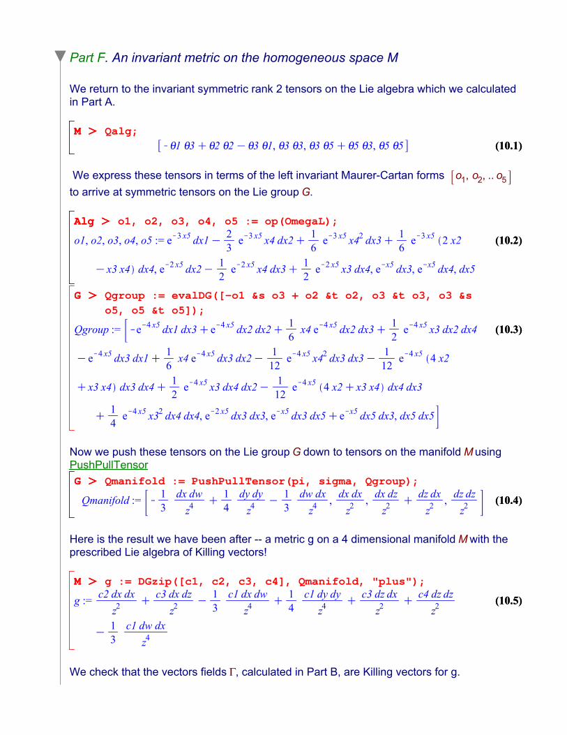
Part F. An invariant metric on the homogeneous space M
We return to the invariant symmetric rank 2 tensors on the Lie algebra which we calculated in Part A.
Qalg;
We express these tensors in terms of the left invariant Maurer-Cartan forms to arrive at symmetric tensors on the Lie group .
o1, o2, o3, o4, o5 := op(OmegaL);
Qgroup := evalDG([-o1 &s o3 + o2 &t o2, o3 &t o3, o3 &s
o5, o5 &t o5]);
Now we push these tensors on the Lie group down to tensors on the manifold usingPushPullTensor
Qmanifold := PushPullTensor(pi, sigma, Qgroup);
Here is the result we have been after -- a metric g on a 4 dimensional manifold with the prescribed Lie algebra of Killing vectors!
g := DGzip([c1, c2, c3, c4], Qmanifold, "plus");
We check that the vectors fields , calculated in Part B, are Killing vectors for g.

(11.1)(11.1)
(10.7)(10.7)
M O M O
M O M O
(8.5)(8.5)
M O M O
(10.6)(10.6)
M O M O
M O M O
(11.2)(11.2)
(5.5)(5.5)
G O G O
(10.9)(10.9)
(6.1.5)(6.1.5)
(10.8)(10.8)
Gamma;
LieDerivative(Gamma, g);
In fact, we can use the KillingVectors program to calculate the Lie algebra of Killing vectors for the metric g.
The result is a 5 dimensional algebra thereby proving that is the full infinitesimal isometry algebra of the metric g.
KV := KillingVectors(g);
GetComponents(KV, Gamma, method = "real", trueorfalse =
"on");true
Part G. Physical properties of the invariant metrics
We calculate the Einstein tensor of our metric. By subtracting an appropriate cosmologicalterm, we conclude that our metric is a pure radiation solution.
Ein := EinsteinTensor(g);
evalDG(Ein - Lambda*InverseMetric(g));

(12.2)(12.2)
M O M O
(12.1)(12.1)
(8.5)(8.5)
(10.6)(10.6)
N O N O
M O M O
(11.2)(11.2)
(5.5)(5.5)
N O N O
G O G O
M O M O
(6.1.5)(6.1.5)
(11.3)(11.3)
(12.3)(12.3)
M O M O
(11.4)(11.4)
M O M O
M O M O
evalDG(Ein - 12/c4*InverseMetric(g));
Note that is a null vector. This means that g is a .
TensorInnerProduct(g, D_w, D_w);0
We find that the Petrov type of our metric is "O".#PetrovType(g);
Part H. Classification of the invariant metric.
Is our pure radiation solution a new solution to the Einstein equations or does it exist in the literature?
We are constructing a very detailed and accurate data base of known solutions and a Maplet to search this database.
Library:-GRExactSolutionsSearch();
So the one candidate we found is in the Exact Solutions Books, Chapter 12, equation 38.Here is the metric.
g38 := Retrieve("Stephani", 1, [12, 38, 2], manifoldname =
M, output = ["Fields"])[1];
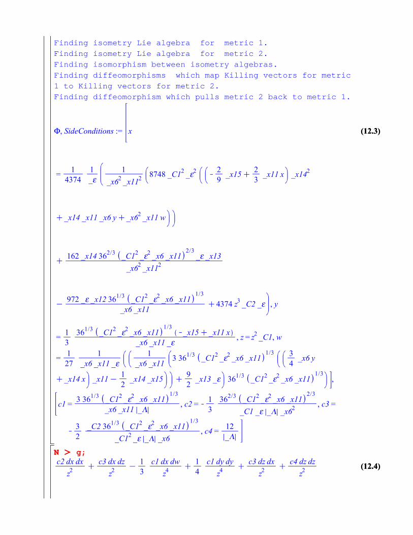
And finally, let us find an explicit diffeomorphism relating these two metrics. We use the EquivalenceOfMetrics command (still under development) and set the infolevel for this command to 2 so we can see what the program is doing.
infolevel[GroupActions:-EquivalenceOfMetrics]:=2;
_EnvExplicit := true:
Phi, SideConditions := GroupActions:-EquivalenceOfMetrics
(g, g38, parameters = {c1, c2, c3, c4});
Finding Killing vectors for metric 1.
Finding Killing vectors for metric 2.
(11.2)(11.2)
(5.5)(5.5)
(8.5)(8.5)
G O G O
N O N O
(6.1.5)(6.1.5)
(10.6)(10.6)
(12.3)(12.3)
(12.4)(12.4)
Finding isometry Lie algebra for metric 1.
Finding isometry Lie algebra for metric 2.
Finding isomorphism between isometry algebras.
Finding diffeomorphisms which map Killing vectors for metric
1 to Killing vectors for metric 2.
Finding diffeomorphism which pulls metric 2 back to metric 1.
g;

N O N O
(8.5)(8.5)
(10.6)(10.6)
(12.4)(12.4)
N O N O
(12.7)(12.7)
(12.6)(12.6)
M O M O
(11.2)(11.2)
(5.5)(5.5)
G O G O
(6.1.5)(6.1.5)
(12.3)(12.3)
(12.5)(12.5)
g1 := PushPullTensor(InverseTransformation(Phi), g);
simplify(subs(SideConditions, g1));
g38;
Perfect.
Note: The Exact Solutions book contains a small error with regards to the metric . The assertation is made that all such metrics are of type N.
SummaryIn this worksheet we
picked a Lie algebra from a database;chose a subalgebra of this Lie algebra and constructed the corresponding homogeneous space;found the invariant metrics on this homogeneous spaceshowed that these metrics solve the Einstein equationslocated this solution is the literature.