An Introduction to Functional Analysis Laurent W. Marcouxlwmarcou/Preprints/LinearAnalysis.pdf · An Introduction to Functional Analysis Laurent W. Marcoux Department of Pure Mathematics

An Introduction to Functional Analysis

Laurent W. Marcoux

Department of Pure MathematicsUniversity of Waterloo

Waterloo, Ontario Canada N2L 3G1

May 24, 2013

Preface to the Third Edition - May 24, 2013

This set of notes is now undergoing its third iteration. The mathematical contentoutside of the appendices is mostly stabilized, and now begins the long and lonelyhunt for typos, poor grammar, and awkward sentence constructions.

Please feel free to contact me if you find any mistakes – mathematical or other-wise – in these notes.

Preface to the Second Edition - December 1, 2010

This set of notes has now undergone its second incarnation. I have corrected asmany typos as I have found so far, and in future instalments I will continue to addcomments and to modify the appendices where appropriate. The course number forthe Functional Analysis course at Waterloo has now changed to PMath 753, in caseanyone is checking.

The comment in the preface to the “first edition” regarding caution and buzzsaws is still a propos. Nevertheless, I maintain that this set of notes is worth at leasttwice the price1 that I’m charging for them.

For the sake of reference: excluding the material in the appendices, and allowingfor the students to study the last section on topology themselves, one should be ableto cover the material in these notes in one term, which at Waterloo consists of 36fifty-minute lectures.

My thanks to Xiao Jiang and Ian Hincks for catching a number of typos that Imissed in the second revision.

1If you were charged a single penny for the electronic version of these notes, you were robbed.You can get them for free from my website.

i

ii

Preface to the First Edition - December 1, 2008

The following is a set of class notes for the PMath 453/653 course I taught at theUniversity of Waterloo in 2008. As mentioned on the front page, they are a work inprogress, and - this being the “first edition” - they are replete with typos. A studentshould approach these notes with the same caution he or she would approach buzzsaws; they can be very useful, but you should be thinking the whole time you havethem in your hands. Enjoy.

I would like to thank Paul Skoufranis for having pointed out to me an embar-rassing number of typos. I am glad to report that he still has both hands and all ofhis fingers.

iii

The reviews are in!

From the moment I picked your book up until I laid it down I wasconvulsed with laughter. Someday I intend reading it.

Groucho Marx

This is not a novel to be tossed aside lightly. It should be thrown withgreat force.

Dorothy Parker

The covers of this book are too far apart.Ambrose Bierce

I read part of it all the way through.Samuel Goldwyn

Reading this book is like waiting for the first shoe to drop.Ralph Novak

Thank you for sending me a copy of your book. I’ll waste no timereading it.

Moses Hadas

Sometimes you just have to stop writing. Even before you begin.Stanislaw J. Lec

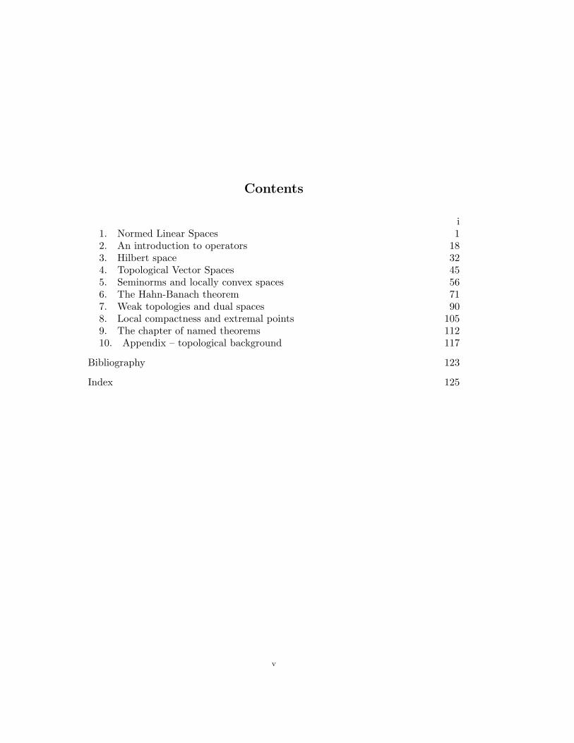
Contents

i1. Normed Linear Spaces 12. An introduction to operators 183. Hilbert space 324. Topological Vector Spaces 455. Seminorms and locally convex spaces 566. The Hahn-Banach theorem 717. Weak topologies and dual spaces 908. Local compactness and extremal points 1059. The chapter of named theorems 11210. Appendix – topological background 117

Bibliography 123

Index 125

v

1. NORMED LINEAR SPACES 1

1. Normed Linear Spaces

I don’t like country music, but I don’t mean to denigrate those who do.And for the people who like country music, denigrate means ‘put down’.

Bob Newhart

1.1. It is expected that the student of this course will have already seen thenotions of a normed linear space and of a Banach space. We shall review thedefinitions of these spaces, as well as some of their fundamental properties. In bothcases, the underlying structure is that of a vector space. For our purposes, thesevector spaces will be over the field K, where K = R or K = C.

1.2. Definition. Let X be a vector space over K. A seminorm on X is a map

ν : X→ R

satisfying

(i) ν(x) ≥ 0 for all x ∈ X;(ii) ν(λx) = |λ| ν(x) for all x ∈ X, λ ∈ K; and

(iii) ν(x+ y) ≤ ν(x) + ν(y) for all x, y ∈ X.

If ν satisfies the extra condition:

(iv) ν(x) = 0 if and only if x = 0,

then we say that ν is a norm, and we usually denote ν(·) by ‖ · ‖. In this case, wesay that (X, ‖ · ‖) (or, with a mild abuse of nomenclature, X) is a normed linearspace.

1.3. A norm on X is a generalisation of the absolute value function on K. Ofcourse, equipped with the absolute value function on K, one immediately defines ametric d : K×K→ R by setting d(x, y) = |x− y|.

In exactly the same way, the norm ‖ · ‖ on a normed linear space X induces ametric

d : X× X → R(x, y) 7→ ‖x− y‖.

The norm topology on (X, ‖ · ‖) is the topology induced by this metric. For eachx ∈ X, a neighbourhood base for this topology is given by

Bx = Dε(x) : ε > 0,

where Dε(x) = y ∈ X : d(y, x) < ε. We say that the normed linear space (X, ‖ · ‖)(or informally X) is complete if the corresponding metric space (X, d) is complete.

2 L.W. Marcoux Functional Analysis

1.4. Example. Define

cK00(N) = (xn)∞n=1 : xn ∈ K, n ≥ 1, xn = 0 for all but finitely many n ≥ 1.For x = (xn)n ∈ cK00(N), set ‖x‖∞ = supn≥1 |xn|. Then (cK00(N), ‖ · ‖∞) is a

normed linear space. It is not, however, complete.The space

cK0 (N) = (xn)∞n=1 : xn ∈ K, n ≥ 1, limn→∞

xn = 0,

equipped with the same norm ‖x‖∞ = supn≥1 |xn| does define a complete normedlinear space.

1.5. Remark. We pause to make a comment about the terminology which weshall be using in these notes. A vector subspace of a vector space V over K isa non-empty subset W for which x, y ∈ W and k ∈ K implies that kx + y ∈ W .When the vector space V does not carry a topology, there is no confusion in thisterminology. When dealing with normed linear spaces (X, ‖ · ‖), and more generallywith the topological vector spaces (V, T ) we shall deal with later in the text, and ofwhich normed linear spaces are an example, one needs to distinguish between thosevector subspaces which are definitely closed sets in the underlying topology fromthose which may or may not be closed. For this reason, we shall refer to vectorsubspaces of a topological vector space (V, T ) which may or may not be closed aslinear manifolds in V, whereas subspaces will be used to denote closed linearmanifolds. As a pedagogical tool, we shall also refer to these as closed subspaces,although strictly speaking, in our language, this is redundant.

Thus cK00(N) is a linear manifold in cK0 (N) under the norm ‖ · ‖∞, but it is not asubspace of cK0 (N), because it is not closed. In fact, it is dense in cK0 (N).

1.6. Example. Consider

PK([0, 1]) = p = p0 + p1z + p2z2 + · · ·+ pnz

n : n ≥ 1, pi ∈ K, 0 ≤ i ≤ n.Then

‖p‖∞ = sup|p(z)| : z ∈ [0, 1]defines a norm on PK([0, 1]). The Stone-Weierstraß Theorem states that PK([0, 1])is a dense linear manifold in the normed linear space C([0, 1],K) of continuous, K-valued functions on [0, 1] with the supremum norm.

If we select x0 ∈ [0, 1] arbitrarily, then it is straightforward to check that ν(f) :=|f(x0)| defines a seminorm on PK([0, 1]) which is not a norm.

1.7. Example. Let n ≥ 1 be an integer. If 1 ≤ p <∞ is a real number, then

‖(x1, x2, ..., xn)‖p =( n∑k=1

|xk|p)1/p

defines a norm on Kn, called the p-norm. We often write `pn for (Kn, ‖ · ‖p), whenthe underlying field K is understood. We may also define

‖(x1, x2, ..., xn)‖∞ = max(|x1|, |x2|, ..., |xn|).


Observe that (Kn, ‖ · ‖∞) is a normed linear space. We abbreviate this to `∞n whenK is understood.

1.8. Example. For 1 ≤ p <∞, we define

`pK(N) = (xn)∞n=1 : xn ∈ K, n ≥ 1 and∞∑n=1

|xn|p <∞.

For (xn)∞n=1 ∈ `pK(N), we set

‖(xn)n‖p =( ∞∑n=1

|xn|p)1/p

.

Then ‖ · ‖p defines a norm, again called the p-norm. on `pK(N).As above, we may also define

`∞K (N) = (xn)∞n=1 : xn ∈ K, n ≥ 1, supn|xn| <∞.

The ∞-norm on `∞K (N) is given by

‖(xn)n‖∞ = supn|xn|.

In most contexts, the underlying field K is understood, and we shall write only`p(N), or even `p, 1 ≤ p ≤ ∞.

The last two examples have one especially nice property not shared by cK00(N)and PK([0, 1]), namely: they are complete.

1.9. Definition. A Banach space is a complete normed linear space.

1.10. Example. Let C([0, 1],K) = f : [0, 1]→ K : f is continuous, equippedwith the uniform norm

‖f‖∞ = max|f(z)| : z ∈ [0, 1].

Then (C([0, 1],K), ‖ · ‖∞) is a Banach space.

1.11. Definition. Let H be an inner product space over K; that is, there existsa map

〈·, ·〉 → Kwhich, for all x, x1, x2, y ∈ H and λ ∈ K, satisfies:

(i) 〈x1 + x2, y〉 = 〈x1, y〉+ 〈x2, y〉;(ii) 〈x, y〉 = 〈y, x〉;(iii) 〈λx, y〉 = λ〈x, y〉;(iv) 〈x, x〉 ≥ 0, with equality holding if and only if x = 0.


(Of course, when K = R, the complex conjugation in (ii) is superfluous.) Recallthat the canonical norm on H induced by the inner product is given by

‖x‖ = 〈x, x〉1/2.If H is complete with respect to the corresponding metric, then we say that H is aHilbert space. Thus every Hilbert space is a Banach space.

1.12. Example. Recall that `2K(N) is a Hilbert space with inner product

〈(xn)n, (yn)n〉 =∞∑n=1

xnyn.

More generally, let (X,µ) be a measure space. Then H = L2(X,µ) is a Hilbertspace with

〈f, g〉 =∫Xfgdµ.

1.13. It is easy to see that if X is a normed linear space, then the vector spaceoperations

σ : X× X → X(x, y) 7→ x+ y

and µ : K× X → X(λ, x) 7→ λx

of addition and scalar multiplication are continuous (from the respective producttopologies on X × X and on K × X to the norm topology on X). The proof is leftas an exercise for the reader. In particular, therefore, if 0 6= λ ∈ K, y ∈ X, thenσy : X → X defined by σy(x) = x + y and µλ : X → X defined by µλ(x) = λx arehomeomorphisms.

As a simple corollary to this fact, a set G ⊆ X is open (resp. closed) if and onlyif G + y is open (resp. closed) for all y ∈ X, and λG is open (resp. closed) for all0 6= λ ∈ K. We shall return to this in a later section.

1.14. New Banach spaces from old. We now exhibit a few constructionswhich allow us to produce new Banach spaces from simpler building blocks.

Let (Xn, ‖ · ‖n)∞n=1 denote a countable family of Banach spaces. Let X =∏n Xn.

(a) For each 1 ≤ p <∞, define∞∑n=1

⊕pXn = (xn)n ∈ X : ‖(xn)n‖p =( ∞∑n=1

‖xn‖pn)1/p

<∞.

Then∑∞

n=1⊕pXn is a Banach space, referred to as the `p-direct sum ofthe (Xn)n.

(b) With p =∞,∞∑n=1

⊕∞Xn = (xn)n ∈ X : ‖(xn)n‖∞ = supn≥1‖xn‖n <∞.

Again,∑∞

n=1⊕∞Xn is a Banach space - namely the `∞-direct sum of the(Xn)n.


(c) We also define

c0(X) = (xn)n ∈ X : xn ∈ Xn, n ≥ 1 and limn→∞

‖xn‖n = 0.

The norm on c0(X) is ‖(xn)n‖∞ = supn≥1 ‖xn‖n, and equipped with thisnorm, c0(X) is easily seen to be a closed subspace of

∑∞n=1⊕∞Xn.

1.15. Definition. Let X be a vector space equipped with two norms ‖ · ‖ and||| · |||. We say that these norms are equivalent if there exist constants κ1, κ2 > 0so that

κ1‖x‖ ≤ |||x||| ≤ κ2‖x‖ for all x ∈ X.

We remark that when this is the case,

1κ2|||x||| ≤ ‖x‖ ≤ 1

κ1|||x|||,

resolving the apparent lack of symmetry in the definition of equivalence of norms.

1.16. Example. Fix n ≥ 1 an integer, and let X = Cn. For x = (x1, x2, ..., xn) ∈X,

‖x‖1 =n∑k=1

|xk| ≤n∑k=1

(maxj|xj |)

=n∑k=1

‖x‖∞ = n‖x‖∞.

Moreover,

‖x‖∞ = maxj|xj | ≤

n∑k=1

|xk| = ‖x‖1,

so that‖x‖∞ ≤ ‖x‖1 ≤ n‖x‖∞.

This proves that ‖ · ‖1 and ‖ · ‖∞ are equivalent norms on X. As we shall later see,all norms on a finite dimensional vector space are equivalent.

1.17. Example. Let X = C([0, 1],C), and consider the norms

‖f‖∞ = sup|f(x)| : x ∈ [0, 1]

and

‖f‖1 =∫ 1

0|f(x)|dx

on X. If, for each n ≥ 1, we set fn to be the function fn(x) = xn, then ‖fn‖∞ = 1,while ‖fn‖1 =

∫ 10 x

ndx = 1n+1 . Clearly ‖ · ‖1 and ‖ · ‖∞ are inequivalent norms on

X.


1.18. Proposition. Two norms ‖·‖ and |||·||| on a vector space X are equivalentif and only if they generate the same metric topologies.Proof. Suppose first that ‖ · ‖ and ||| · ||| are equivalent, say κ1‖x‖ ≤ |||x||| ≤ κ2‖x‖for all x ∈ X, where κ1, κ2 > 0 are constants. If x ∈ X and (xn)n is a sequence inX, then it immediately follows that

limn→∞

‖xn − x‖ = 0 if and only if limn→∞

|||xn − x||| = 0.

That is, the two notions of convergence coincide, and thus the topologies are equal.

Conversely, suppose that the metric topologies τ‖·‖ and τ|||·|||, induced by ‖ · ‖and ||| · ||| respectively, coincide. Then G = x ∈ X : ‖x‖ < 1 is an open nbhd of 0in (X, ||| · |||), and so there exists δ > 0 so that H = x ∈ X : |||x||| < δ ⊆ G. Thatis, |||x||| < δ implies ‖x‖ < 1. In particular, therefore, |||x||| ≤ δ/2 implies ‖x‖ ≤ 1,so that that ||y|| ≤ (2/δ)|||y||| for all y ∈ X. By symmetry, there exists a constantκ2 > 0 so that |||y||| ≤ κ2‖y‖ for all y ∈ X.

Thus ‖ · ‖ and ||| · ||| are equivalent norms.

2

1.19. Corollary. Equivalence of norms is an equivalence relation for norms ona vector space X.

1.20. Definition. Let (X, ‖ · ‖) be a normed linear space. A series∑∞

n=1 xn inX is said to be absolutely summable if

∑∞n=1 ‖xn‖ <∞.

The following result provides a very practical tool when trying to decide whetheror not a given normed linear space is complete. We remark that the second half ofthe proof uses the standard fact that if (yn)n is a Cauchy sequence in a metric space(Y, d), and if (yn)n admits a convergent subsequence with limit y0, then the originalsequence (yn)n converges to y0 as well.

1.21. Proposition. Let (X, ‖ · ‖) be a normed linear space. The followingstatements are equivalent:

(a) X is complete, and hence X is a Banach space.(b) Every absolutely summable series in X is summable.

Proof.

(a) implies (b): Suppose that X is complete, and that∑xn is absolutely

summable. For each k ≥ 1, let yk =∑k

n=1 xn. Given ε > 0, we can find


N > 0 so that m ≥ N implies∑∞

n=m ‖xn‖ < ε. If k ≥ m ≥ N , then

‖yk − ym‖ = ‖k∑

n=m+1

xn‖

≤k∑

n=m+1

‖xn‖

≤∞∑

n=m+1

‖xn‖

< ε,

so that (yk)k is Cauchy in X. Since X is complete, y = limk→∞ yk =limk→∞

∑kn=1 xn =

∑∞n=1 xn exists, i.e.

∑∞n=1 xn is summable.

(b) implies (a): Next suppose that every absolutely summable series in X issummable, and let (yj)j be a Cauchy sequence in X. For each n ≥ 1 thereexists Nn > 0 so that k,m ≥ Nn implies ‖yk−ym‖ < 1/2n+1. Let x1 = yN1

and for n ≥ 2, let xn = yNn − yNn−1 . Then ‖xn‖ < 1/2n for all n ≥ 2, sothat

∞∑n=1

‖xn‖ ≤ ‖x1‖+∞∑n=2

12n

≤ ‖x1‖+12<∞.

By hypothesis, y =∑∞

n=1 xn = limk→∞∑k

n=1 xn exists. But∑kn=1 xn = yNk , so that limk→∞ yNk = y ∈ X. Recalling that (yj)j was

Cauchy, we conclude from the remark preceding the Proposition that (yj)jalso converges to y. Since every Cauchy sequence in X converges, X iscomplete.

2

1.22. Theorem. Let (X, ‖ · ‖) be a normed linear space, and let M ⊆ X be alinear manifold. Then

p(x+ M) := inf‖x+m‖ : m ∈M

defines a seminorm on the quotient space X/M.This formula defines a norm on X/M if and only if M is closed.

Proof. First observe that the function p is well-defined; for if x+ M = y+ M, thenx− y ∈M and so

p(y + M) = inf‖y +m‖ : m ∈M= inf‖y +m+ (x− y)‖ = ‖x+m‖ : m ∈M= p(x+ M).


Clearly p(x + M) ≥ 0 for all x + M ∈ X/M. If 0 6= k ∈ K, then m ∈M if andonly if 1

km ∈M and so

p(k(x+ M)) = p(kx+ M)

= inf‖kx+m‖ : m ∈M

= inf‖k(x+1km)‖ : m ∈M

= |k| inf‖x+m0‖ : m0 ∈M= |k|p(x+ M).

If k = 0, then p(0 + M) = 0, since m = 0 ∈M.Finally,

p((x+ M) + (y + M)) = p(x+ y + M)

= inf‖(x+ y) +m‖ : m ∈M= inf‖(x+m1) + (y +m2)‖ : m1,m2 ∈M≤ inf‖x+m1‖+ ‖y +m2‖ : m1,m2 ∈M= p(x+ M) + p(y + M).

In the case where M is closed in X, suppose that p(x+ M) = 0 for some x ∈ X.Then

inf‖x+m‖ : m ∈M = 0,

so there exist mn ∈M, n ≥ 1, so that −x = limn→∞mn. Since M is closed, −x ∈Mand so x+ M = x+ (−x) + M = 0 + M, proving that p is a norm.

The converse statement is left as an exercise.

2

1.23. Let X be a normed linear space and M be a linear manifold in X. We shalldenote the canonical quotient map from X to X/M by q (or qM if the need to bespecific arises). When M is closed in X, we shall denote the norm from Theorem 1.22once again by ‖ · ‖ (or ‖ · ‖X/M), so that

‖q(x)‖ = ‖x+ M‖ = inf‖x+m‖ : m ∈M.

It is clear that ‖q(x)‖ ≤ ‖x‖ for all x ∈ X, and so q is continuous. Indeed, givenε > 0, we can take δ = ε to get ‖x − y‖ < δ implies ‖q(x) − q(y)‖ ≤ ‖x − y‖ < ε.We shall see below that q is also an open map - i.e. it takes open sets to open sets.

1.24. Theorem. Let X be a normed linear space and M be a closed subspaceof X.

(a) If X is complete, then so are M and X/M.(b) If M and X/M are complete, then so is X.

Proof.


(a) Suppose that X is complete. We first show that M is complete.Let (mn)∞n=1 be a Cauchy sequence in M. Then it is Cauchy in X and

X is complete, so that x = limn→∞mn ∈ X. Since M is closed in X, x ∈M.Thus M is complete.

Note that this argument shows that any closed subset of a completemetric space is complete.

Next we show that X/M is also complete.Let

∑n q(xn) be an absolutely summable series in X/M. For each

n ≥ 1, choose mn ∈M so that ‖xn +mn‖ ≤ ‖q(xn)‖+ 12n . Then∑

n

‖xn +mn‖ ≤∑n

(‖q(xn)‖+

12n

)<∞,

so∑

n(xn +mn) is summable in X since X is complete. Set

x0 :=∑n

(xn +mn).

By the continuity of q,

q(x0) = q(∑n

(xn +mn))

=∑n

q(xn +mn)

=∑n

q(xn).

Thus every absolutely summable series in X/M is summable, and so byProposition 1.21, X/M is complete.

(b) Suppose next that M and X/M are both complete.Let (xn)∞n=1 be a Cauchy sequence in X. Then (q(xn))∞n=1 is Cauchy in

X/M and thus q(y) = limn→∞ q(xn) exists, by the completeness of X/M.For n ≥ 1, choose mn ∈M so that

‖y − (xn +mn)‖ < ‖q(y)− q(xn)‖+12n.

Since (xn + mn)∞n=1 converges to y in X, it follows that it is a Cauchysequence. Since both (xn)∞n=1 and (xn+mn)∞n=1 are Cauchy, it follows that(mn)∞n=1 is also Cauchy – a fact that follows easily from the observationthat

‖mj −mi‖ ≤ ‖(xj +mj)− (xi +mi)‖+ ‖xj − xi‖.But M is complete and so m := limn→∞mn ∈M. This yields

y −m = limn→∞

(xn +mn)−m = limn→∞

xn,

so that (xn)∞n=1 converges to y −m in X. That is, X is complete.2


1.25. Proposition. Let X be a normed linear space and M be a closed subspaceof X. Let q : X→ X/M denote the canonical quotient map.

(a) A subset W ⊆ X/M is open if and only if q−1(W ) is open in X.(b) The map q is an open map - i.e., if G ⊆ X is open, then q(G) is open in

X/M.Proof.

(a) If W ⊆ X/M is open, then q−1(W ) is open in X because q is continuous.Suppose next that W ⊆ X/M and that q−1(W ) is open in X. Let

q(x) ∈ W . Then x ∈ q−1(W ), and so we can find δ > 0 so that Vδ(x) ⊆q−1(W ). If ‖q(y)− q(x)‖ < δ, then ‖y − x+m‖ < δ for some m ∈M, andthus q(y) = q(y + m) ∈ q(Vδ(x)) ⊆ W . That is, Vδ(q(x)) ⊆ W , and W isopen.

(b) Let G ⊆ X be an open set. Observe that q−1(q(G)) = G+M = ∪m∈MG+mis open, being the union of open sets. By (a), q(G) is open.

2

1.26. Let M be a finite-dimensional linear manifold in a normed linear spaceX. Then M is closed in X. The proof of this is left as an assignment exercise.

1.27. Proposition. Let X be a normed linear space. If M and Z are closedsubspaces of X and dim Z <∞, then M + Z is closed in X.Proof. Let q : X → X/M denote the canonical quotient map. Since Z is a finitedimensional vector space, so is q(Z). By the exercise preceding this Proposition,q(Z) is closed in X/M. Since q is continuous, M + Z = q−1(q(Z)) is closed in X.

2


Appendix to Section 1.

1.28. This course assumes that the reader has taken at least enough Real Anal-ysis to have seen that (`pK(N), ‖ · ‖p) is a normed linear space for each 1 ≤ p ≤ ∞.Having said that, let us review Holder’s Inequality as well as Minkowski’s Inequalityin this setting, since Holder’s Inequality is also useful in studying dual spaces in thenext Section. The reader will recall that Minkowski’s Inequality is the statementthat the p-norm is subadditive; that is, that the p-norm satisfies condition (iii) ofDefinition 1.2. We remark that both inequalities hold for more general Lp-spaces.Our decision to concentrate on `p-spaces instead of their more general counterpartsis an attempt to accommodate the background of the students who took this course,as opposed to a conscious effort to avoid Lp-spaces.

Before proving Holder’s Inequality, we pause to prove the following Lemma.

1.29. Lemma. Let a and b be positive real numbers and suppose that1 < p, q <∞ satisfy 1

p + 1q = 1. Then

a1p b

1q ≤ a

p+b

q.

Proof. Let 0 < t < 1 and consider the function

f(x) = xt − tx+ t− 1,

defined on (0,∞). Then

f ′(x) = txt−1 − t = t(xt−1 − 1).

Thus f(1) = 0 = f ′(1). Since f ′(x) > 0 for x ∈ (0, 1) and f ′(x) < 0 for x ∈ (1,∞),it follows that

f(x) < f(1) = 0 for all x 6= 1.That is, xt ≤ (1− t) + tx for all x > 0, with equality holding if and only if x = 1.

Letting x = a/b, t = 1/p yields

a1p b

1q−1 = a

1p b−1p

= (a

b)

1p

≤ (1− 1p

) +1p

(a

b)

=1p

(a

b) +

1q.

Multiplying both sides of the equation by b yields the desired inequality.2


1.30. Theorem. Holder’s InequalityLet 1 ≤ p, q ≤ ∞, and suppose that 1

p + 1q = 1. Let x = (xn)n ∈ `p and

y = (yn)n ∈ `q. If z = (zn)n, where zn = xnyn for all n ≥ 1, then z ∈ `1 and

‖z‖1 ≤ ‖x‖p ‖y‖q.

Proof. The cases where p = 1 or p =∞ are routine and are left to the reader.First let us suppose that ‖x‖p = ‖y‖q = 1. Applying the previous Lemma to

our sequences x and y yields, for each n ≥ 1,

|xnyn| = (|xn|p)1p (|yn|q)

1q

≤ 1p|xn|p +

1q|yn|q,

so that ∑n

|zn| =∑n

|xnyn|

≤ 1p

∑n

|xn|p +1q

∑n

|yn|q

=1p‖x‖pp +

1q‖y‖qq

= 1.

In general, if x ∈ `p and y ∈ `q, let u = x/(‖x‖p), v = v/(‖y‖q) so that‖u‖p = 1 = ‖v‖q and so

1‖x‖p ‖y‖q

∑n

|xnyn| =∑n

|unvn|

≤ 1.

Thus‖z‖1 ≤ ‖x‖p ‖y‖q.

2

Holder’s Inequality is the key to proving Minkowski’s Inequality.

1.31. Theorem. Minkowski’s Inequality.Let 1 ≤ p ≤ ∞, and suppose that x = (xn)n and y = (yn)n are in `p. Then

x+ y = (xn + yn)n ∈ `p and

‖x+ y‖p ≤ ‖x‖p + ‖y‖p.

Proof. Again, the cases where p = 1 and where p = ∞ are left to the reader.Suppose therefore that 1 < p <∞. Observe that if a, b > 0, then(

a+ b

2

)p≤ ap + bp,


so that (a+ b)p ≤ 2p(ap + bp). It follows that∑n

|xn + yn|p ≤ 2p∑n

(|xn|p + |yn|p) <∞,

which proves that x+ y ∈ `p.By Holder’s Inequality,∑

n

|xn + yn|p−1 |xn| ≤ ‖x‖p ‖(|xn + yn|p−1)n‖q,

and similarly ∑n

|xn + yn|p−1 |yn| ≤ ‖y‖p ‖(|xn + yn|p−1)n‖q.

Now

‖(|xn + yn|p−1)n‖q =

(∑n

|xn + yn|(p−1)q

) 1q

=

(∑n

|xn + yn|(pq−q)) 1

q

=

(∑n

|xn + yn|p) 1

q

= ‖(xn + yn)n‖p/qp .

Hence

‖x+ y‖pp =∑n

|xn + yn| |xn + yn|p−1

≤∑n

(|xn|+ |yn|) |xn + yn|p−1

≤ (‖x‖p + ‖y‖p) ‖(|xn + yn|p−1)n‖q= (‖x‖p + ‖y‖p) ‖(xn + yn)n‖p/q,

from which we get

‖x+ y‖p = ‖x+ y‖p−p/qp ≤ ‖x‖p + ‖y‖p.

2

Let us now examine a couple of examples of useful Banach spaces whose defi-nitions require a somewhat better background in Analysis than we are assuming inthe main body of the text.


1.32. Example. Let x = (xn)n be a sequence of complex (or real) numbers.The total variation of x is defined by

V (x) :=∞∑n=1

|xn+1 − xn|.

If V (x) <∞, we say that x has bounded variation. The space

bv := (xn)n : xn ∈ K, n ≥ 1, V (x) <∞is called the space of sequences of bounded variation. We may define a normon bv as follows: for x ∈ bv, we set

‖(xn)n‖bv := |x1|+ V (x) = |x1|+∞∑n=1

|xn+1 − xn|.

It can be shown that bv is complete under this norm, and hence that bv is aBanach space.

If we let bv0 = (xn)n ∈ bv : limn→∞ xn = 0, then

‖(xn)n‖bv0 := V ((xn)n)

defines a norm on bv0, and again, bv0 is a Banach space with respect to this norm.

1.33. Example. The geometric theory of real Banach spaces is an active andexciting area. For a period of time, the following question was open [Lin71]: doesevery infinite-dimensional Banach space contain a subspace which is linearly home-omorphic to one of the spaces `p, 1 ≤ p <∞ or c0? In 1974, B.S. Tsirel’son [Tsi74]provided a counterexample to this conjecture. In this example, we shall discussthe broad outline of the construction of the Tsirel’son space, omitting the proofs ofcertain technical details.

We begin by considering the space c0 of Example 1.4. For each n ≥ 1, let en ∈ c0

denote the sequence (0, 0, ..., 0, 1, 0, 0, ...), with the unique “1” occurring in the nth

coordinate. Given x = (xn)n ∈ c0, we may write x =∑∞

n=1 xnen. Let us also definethe map Pn : c0 → c0 via Pn(xk)k := (0, 0, ..., 0, xn+1, xn+2, xn+3, ...).

Given a finite set v1, v2, ..., vr of vectors in c0, we shall say that they are block-disjoint for consecutively supported – written v1 < v2 < · · · < vr – if there existα1, α2, ..., αr, β1, β2, ..., βr ∈ N with

α1 ≤ β1 < α2 ≤ β2 < · · · < αr ≤ βrso that supp(vj) ⊆ [αj , βj ], 1 ≤ j ≤ r. Here, for x = (xn)n ∈ c0,

supp(x) := j ∈ N : xj 6= 0.We shall write (v1, v2, ..., vr) for

∑rj=1 vj when v1 < v2 < · · · < vr.

For a subset B ⊆ c0, we consider the following set of conditions which B may ormay not possess:

(a) x ∈ B implies that ‖x‖∞ ≤ 1; i.e. B is contained in the unit ball of c0.


(b) en∞n=1 ⊆ B.(c) If x =

∑∞n=1 xnen ∈ B, y = (yn)n ∈ c0 and |yn| ≤ |xn| for all n ≥ 1, then

y ∈ B. (This is a hereditary property.)(d) If v1 < v2 < · · · < vr lie in B, then 1

2Pr((v1, v2, ..., vr)) ∈ B.(e) For every x ∈ B there exists n ∈ N for which 2Pn(x) ∈ B.

Our first goal is to construct a set K which has all five of these properties.Let L1 = rej : −1 ≤ r ≤ 1, j ≥ 1 and for n ≥ 1, set

Ln+1 = Ln ∪ 12Pr((v1, v2, ..., vr)) : r ≥ 1, v1 < v2 < · · · < vr ∈ Ln.

Let K denote the pointwise closure of ∪n≥1Ln. It can be shown that K ⊆ c0. Weset D = co(K) denote the closed convex hull of K (with the closure taking place inc0).

The Tsirel’son space T is then defined as spanD. The norm on T is given bythe Minkowski functional which we shall encounter later when studying locallyconvex spaces. It is given by ‖x‖T = infr ∈ (0,∞) : x ∈ rD, where rD = ry :y ∈ D. As we shall later see, the definition of this norm ensures that D is preciselythe unit ball of T .

Although we shall not prove it here, (T, ‖ · ‖T ) is a Banach space which does notcontain any copy of c0 or `p, 1 ≤ p <∞.

1.34. Example. Another Banach space of interest to those who study thegeometry of said spaces is James’ space.

For a sequence (xn)n of real numbers, consider the following condition, whichwe shall call condition J : for all k ≥ 1,

supn1<n2<···<nk

[(xn1 − xn2)2 + (xn2 − xn3)2 + · · ·+ (xnk−1

− xnk)2]<∞.

The James’ space is defined to be:

J = (xn)n ∈ c0 : (xn)n satisfies condition J.

The norm on J is defined via:

‖(xn)n‖J := supn1<n2<···<nk

[(xn1 − xn2)2 + (xn2 − xn3)2 + · · ·+ (xnk−1

− xnk)2] 1

2 .

It can be shown that J is a Banach space when equipped with this norm.

1.35. Example. Let X be a locally compact topological space and let B denotethe σ–algebra of Borel subsets of X. Let µ be a positive measure on X, so that

µ : B → R ∪ ∞

satisfies(a) µ(∅) = 0;(b) µ(B) ≥ 0 for all B ∈ B;


(c) if Bnn is a sequence of disjoint, measurable subsets from B, then

µ(∪nBn) =∑n

µ(Bn).

The measure µ is said to be finite if µ(X) <∞, and it is said to be regular if(i) µ(K) <∞ for all compact subsets K ∈ B;

(ii) µ(B) = supµ(K) : K ⊆ B,K compact for all B ∈ B; and(iii) µ(B) = infµ(G) : B ⊆ G,G open for all B ∈ B.A complex-valued, Borel measure on X is a function

ν : B → Csatisfying:

(a) ν(∅) = 0, and(b) if Bnn is a sequence of disjoint, measurable subsets from B, then

ν(∪nBn) =∑n

ν(Bn).

Let ν be a complex-valued Borel measure on X. For each B ∈ B, a measurablepartition of B is a finite collection E1, E2, ..., Ek of disjoint, measurable setswhose union is B. We define the variation |ν| of ν to be the function defined asfollows: for B ∈ B,

|ν|(B) := supk∑j=1

|ν(Ej)| : Ejkj=1 is a measurable partition of B.

It is routine to verify that |ν| is then a finite, positive Borel measure on X. Wesay that ν is regular if |ν| is.

It is clear that every complex-linear combination of finite, positive, regular Borelmeasures yields a complex-valued, regular Borel measure on X. A standard resultfrom measure theory known as the Hahn-Jordan Decomposition Theoremstates that the converse holds, namely: every complex-valued, regular Borel measurecan be written as a complex-linear combination of (four) finite, positive, regularBorel measures.

Let MC(X) denote the complex vector space of all complex-valued, regular Borelmeasures on X. Then the map

‖ · ‖ : MC(X) → [0,∞)ν 7→ |ν|(X)

defines a norm on MC(X), and MC(X) is complete with respect to this norm.

1.36. In Theorem 1.24, we showed that if X is a Banach space and M is a closedsubspace, then X/M is complete. Our proof there was based upon Proposition 1.21.This result also admits a direct proof in terms of Cauchy sequences:

Theorem. Let X be a Banach space and suppose that M is a closed subspace ofX. Then X/M is complete.


Proof.Let (q(xn))∞n=1 be a Cauchy sequence in X/M. For each n ≥ 1, there exists

kn > 1 so that i, j ≥ kn implies ‖q(xi) − q(xj)‖ < 2−n. Without loss of generality,we may assume that kn > kn−1 for all n ≥ 2.

Set zn := xkn , n ≥ 1 and let m1 = 0. For n > 1, choose mn ∈M so that

‖(zn−1 +mn−1)− (zn +mn)‖ < 2−(n−1).

That this is possible follows from the definition of the quotient norm along with theinequality of the second paragraph. If we now define yn := zn + mn, n ≥ 1, thenq(yn) = q(zn) = q(xkn), and for n2 > n1,

‖yn1 − yn2‖ ≤n2−n1∑j=1

‖yn1+j − yn1+j−1‖

≤n2−n1∑j=1

(12

)(n1+j−1)

≤∞∑j=0

(12

)(n1+j)

= (12

)n1−1,

from which it follows that (yn)∞n=1 is Cauchy in X. Since X is complete, y :=limn→∞ yn ∈ X, and since the quotient norm is contractive, q(y) = limn→∞ q(yn) =limn→∞ q(xkn). Since (q(xn))∞n=1 is Cauchy, q(y) = limn→∞ q(xn), which provesthat every Cauchy sequence in X/M converges - i.e. that X/M is complete.

2

∗

I have the body of an eighteen year old. I keep it in the fridge.Spike Milligan


2. An introduction to operators

Some people are afraid of heights. Not me, I’m afraid of widths.Steven Wright

2.1. The study of mathematics is the study of mathematical objects and therelationships between them. These relationships are often measured by functionsfrom one object to another. Of course, when both objects belong to the samecategory (be it the category of vector spaces, groups, rings, etc), it is to be expectedthat the most important maps between these objects will be morphisms from thatcategory. In this Section we shall concern ourselves with bounded linear operatorsbetween normed linear spaces. These bounded linear maps, as we shall soon discover,coincide with those linear maps which are continuous in the norm topology. Sincenormed linear spaces are vector spaces equipped with a norm topology, the boundedlinear operators are the natural morphisms between them.

It should be pointed out that Banach spaces can be quite complicated to analyze.For this reason, many people working in this area often study the structure andgeometry of these spaces without necessarily emphasizing the study of the linearmaps between them. In the next Section we shall examine the notion of a Hilbertspace. These are amongst the best-behaved Banach spaces, and their structureis relatively well understood. For this reason, fewer people study Hilbert spacesalone; Hilbert space theory tends to focus on the theory of the bounded linear mapsbetween them, as well as algebras of such bounded linear operators.

We would also be remiss if we failed to point out that not everyone on the planetrestricts themselves to bounded (i.e. continuous) linear operators. Differentiationhas the grave misfortune of being an unbounded linear operator, but neverthelessit is hard to avoid if one wishes to study the world around one - or around one’sfriends, acquaintances, enemies, and every other one. Indeed, in applied mathemat-ics and physics, it is often the case that the unbounded linear operators are the moreinteresting examples. Having said that, we shall leave it to the disciples of thoseschools to wax poetic on these topics.

2.2. Definition. Let X and Y be normed linear spaces, and let T : X → Ybe a linear map. We say that T is a bounded operator if there exists a constantk ≥ 0 so that ‖Tx‖ ≤ k‖x‖ for all x ∈ X. When T is bounded, we define

‖T‖ = infk ≥ 0 : ‖Tx‖ ≤ k‖x‖ for all x ∈ X.

We shall refer to ‖T‖ as the operator norm of T .It is, of course, understood that the norm of Tx is computed using the Y-norm,

while the norm of x is computed using the X-norm. As we shall see below, theoperator norm does define a bona fide norm on the vector space of bounded linearmaps from X to Y, thereby justifying our terminology.

2. AN INTRODUCTION TO OPERATORS 19

Our interest in bounded operators stems from the fact that they are preciselythe continuous operators from X to Y.

2.3. Theorem. Let X and Y be normed linear spaces and T : X → Y be alinear map. The following are equivalent:

(a) T is continuous on X.(b) T is continuous at 0.(c) T is bounded.(d) κ1 := sup‖Tx‖ : x ∈ X, ‖x‖ ≤ 1 <∞.(e) κ2 := sup‖Tx‖ : x ∈ X, ‖x‖ = 1 <∞.(f) κ3 := sup‖Tx‖/‖x‖ : 0 6= x ∈ X <∞.

Furthermore, if any of these holds, then κ1 = κ2 = κ3 = ‖T‖.Proof.

(a) implies (b): This is trivial.(b) implies (c): Suppose that T is continuous at 0. Let ε = 1 and choose δ > 0

so that ‖x− 0‖ < δ implies that ‖Tx− T0‖ = ‖Tx‖ < ε = 1. If ‖y‖ ≤ δ/2,then ‖Ty‖ ≤ 1, and so ‖x‖ ≤ 1 implies ‖T

(δ2x)‖ ≤ 1, i.e. ‖Tx‖ ≤ 2/δ.

Thus ‖T‖ ≤ 2/δ <∞, and T is bounded.(c) implies (d): This is trivial.(d) implies (e): This is trivial.(e) implies (f): Again, this is trivial.(f) implies (a): Observe that for any x ∈ X, ‖Tx‖ ≤ κ2‖x‖. (For x 6= 0, this

follows from the hypothesis, while the linearity of T implies that T0 = 0, sothe inequality also holds for x = 0.) Thus if ε > 0 and ‖x−y‖ < ε/(κ2 +1),then

‖Tx− Ty‖ = ‖T (x− y)‖ ≤ κ2‖x− y‖ < ε.

The proof of the final statement is left as an exercise for the reader.2

2.4. Computing the operator norm of a given operator T is not always a simpletask. For example, suppose that H = (C2, ‖ · ‖2) is a two-dimensional Hilbertspace with standard orthonormal basis e1 = (1, 0), e2 = (0, 1). Let T : H → H

be the map whose matrix with respect to this basis is[1 23 4

], so that T (x, y) =

(x+ 2y, 3x+ 4y). By definition,

‖T‖ = sup‖Tz‖ : z ∈ C2, ‖z‖ ≤ 1

= sup√|x+ 2y|2 + |3x+ 4y|2 : x, y ∈ C,

√|x|2 + |y|2 ≤ 1,

which involves non-linear equations. For Hilbert spaces of low dimension – say,less than dimension 5 – alternate methods exist (but won’t be developed just yet).Instead, we turn our attention to special classes of operator which are simple enoughto allow us to obtain interesting results.

So as to satisfy the curious reader, we mention that the norm of T is√

15 +√

221.


2.5. Example. Multiplication operators.(a) Let X =

(C([0, 1],C), ‖ · ‖∞

), and suppose that f ∈ X. Define

Mf : X → Xg 7→ fg

.

It is routine to check that Mf is linear. If ‖g‖∞ ≤ 1, then

‖Mfg‖∞ = ‖fg‖∞ = sup|f(x)g(x)| : x ∈ [0, 1] ≤ ‖f‖∞ ‖g‖∞.

Thus ‖Mf‖∞ ≤ ‖f‖∞ <∞, and Mf is bounded.Setting g(x) = 1, x ∈ [0, 1], we have g ∈ X, ‖g‖∞ = 1 and ‖Mfg‖∞ =

‖f‖∞, so that ‖Mf‖ ≥ ‖f‖∞ and therefore ‖Mf‖ = ‖f‖∞.For (hopefully) obvious reasons, Mf is referred to as a multiplication

operator .(b) We now consider a similar operator acting on a Hilbert space. Let H =

L2(X, dµ), where dµ is a positive, regular Borel measure. Suppose thatf ∈ L∞(X, dµ) and let

Mf : X → Xg 7→ fg

.

Once again, it is easy to check that Mf is linear, while for g ∈ H,

‖Mfg‖2 =( ∫ 1

0|f(x)g(x)|2dµ

) 12

≤( ∫ 1

0‖f‖2∞|g(x)|2dµ

) 12

= ‖f‖∞ ‖g‖2,

so that ‖Mf‖ ≤ ‖f‖∞, and hence Mf is bounded. As for a lower bound onthe norm of Mf , for each n ≥ 1, let Fn = x ∈ X : |f(x)| ≥ ‖f‖∞ − 1/n.Then Fn is measurable and µ(Fn) > 0 by definition of ‖f‖∞. Let En ⊆ Fnbe a measurable set for which 0 < µ(En) < ∞, n ≥ 1. The existence ofsuch sets En, n ≥ 1 follows from the regularity of the measure µ. Letgn = χEn , the characteristic function of En. Then gn ∈ L2(X,µ) for alln ≥ 1 and

‖Mfgn‖2 =( ∫ 1

0|f(x)gn(x)|2dµ

) 12

=( ∫

En

|f(x)|2dµ) 1

2

≥( ∫

En

(‖f‖∞ − 1/n)2dµ) 1

2

=(‖f‖∞ − 1/n

) ( ∫ 1

0|gn(x)|dµ

) 12

=(‖f‖∞ − 1/n

)‖gn‖2.


From this we see that ‖Mf‖ ≥ ‖f‖∞ − 1/n. Since n ≥ 1 was arbitrary,‖Mf‖ ≥ ‖f‖∞, and so ‖Mf‖ = ‖f‖∞.

Observe that the computation of the norm of the operator dependedvery much upon the underlying norms of the spaces involved.

(c) As a special case of this phenomenon, let X = N and suppose that dµ iscounting measure. Then H = `2(N) and f ∈ `∞(N). As we are wont todo when dealing with sequences, we denote by dn the value f(n) of f atn ∈ N, so that f ≡ (dn)∞n=1 ∈ `∞(N). It follows that Mf (xn)n = (dnxn)nfor all (xn)n ∈ `2(N). By considering the matrix [Mf ] of Mf with respectto the standard orthonormal basis (en)n for H, we see that

[Mf ] =

d1

d2

d3

. . .

.Thus, Mf , often denoted in this circumstance as D = diagdnn, is referredto as a diagonal operator . The above calculation shows that

‖D‖ = ‖Mf‖ = ‖f‖∞ = sup|f(n)| : n ≥ 1 = sup|dn| : n ≥ 1.

2.6. Example. Weighted shifts. With H = `2(N) and (wn)n ∈ `∞(N),consider the map W : H → H defined by

W (xn)n = (0, w1x1, w2x2, w3x3, ...) for all (xn)n ∈ `2(N).

We leave it as an exercise for the reader to show that W is a bounded linear operatoron H, and that

‖W‖ = sup|wn| : n ≥ 1.

Such an operator is referred to as a unilateral forward weighted shift.If (vn)n ∈ `∞(N) and we define the linear map V : H → H via

V (xn)n = (v1x2, v2x3, v3x4, ...) for all (xn)n ∈ H,

then once again V is bounded, ‖V ‖ = sup|vn| : n ≥ 1, and V is referred to as aunilateral backward weighted shift.

Finally, consider H = `2(Z), and with (un)n ∈ `∞(Z), define the linear mapU : H → H via

U(xn)n = (un−1xn−1)n.

Again, U is bounded with ‖U‖ = sup|un| : n ∈ Z, and U is referred to as abilateral weighted shift. The reader should ask himself/herself why we do notrefer to “forward” and “backward” bilateral shift operators.


2.7. Example. Differentiation operators. Consider the linear manifoldP(D) = p : p a polynomial ⊆ (C(D), ‖ · ‖∞). Define the map

D : P(D) → P(D)p 7→ p′,

the derivative of p. Then if pn(z) = zn, ‖pn‖∞ = 1 for each n ≥ 1 and Dpn =npn−1, whence ‖D‖ ≥ n for all n ≥ 1. In particular, D is not bounded. That is,differentiation is not continuous on the linear space of polynomials.

2.8. Notation. The set of bounded linear operators from the normed linearspace X to the normed linear space Y is denoted by B(X,Y). If X = Y, we abbreviatethis to B(X). We now fulfil an earlier promise by proving that the map T 7→ ‖T‖does indeed define a norm on B(X,Y).

2.9. Proposition. Let X and Y be normed linear spaces. Then B(X,Y) is avector space and the operator norm is a norm on B(X,Y).Proof. Since linear combinations of continuous functions between topological spacesare continuous, B(X,Y) is a vector space.

As to the second assertion: for R, T ∈ B(X,Y) and k ∈ K,(i) ‖T‖ = sup‖Tx‖ : ‖x‖ ≤ 1 ≥ 0;

(ii) ‖T‖ = 0 if and only if ‖Tx‖/‖x‖ = 0 for all x 6= 0, which in turn happensif and only if Tx = 0 for all x ∈ X; i.e. if and only if T = 0.

(iii)

‖kT‖ = sup‖kTx‖ : ‖x‖ ≤ 1= sup|k| ‖Tx‖ : ‖x‖ ≤ 1= |k| sup‖Tx‖ : ‖x‖ ≤ 1= |k| ‖T‖.

(iv)

‖R+ T‖ = sup‖(R+ T )x‖ : ‖x‖ ≤ 1≤ sup‖Rx‖+ ‖Tx‖ : ‖x‖ ≤ 1≤ sup‖Rx‖+ ‖Ty‖ : ‖x‖, ‖y‖ ≤ 1= ‖R‖+ ‖T‖.

This completes the proof.2

2.10. Theorem. Let X and Y be normed linear spaces and suppose that Y iscomplete. Then B(X,Y) is complete, and as such it is a Banach space.Proof. Suppose that

∑∞n=1 Tn is an absolutely summable series in B(X,Y). Given

x ∈ X,∞∑n=1

‖Tnx‖ ≤∞∑n=1

‖Tn‖ ‖x‖ = ‖x‖( ∞∑n=1

‖Tn‖)<∞,


and thus, since Y is compete,∑∞

n=1 Tnx ∈ Y exists. Moreover, the linearity of eachTn implies that the map T : X → Y defined via Tx =

∑∞n=1 Tnx is linear, while

‖x‖ ≤ 1 implies from above that ‖Tx‖ ≤∑∞

n=1 ‖Tn‖. Hence

‖T‖ ≤∞∑n=1

‖Tn‖ <∞,

implying that T is bounded.Finally,

‖Tx−N∑n=1

Tnx‖ = ‖∞∑

n=N+1

Tnx‖

≤ ‖x‖∞∑

n=N+1

‖Tn‖,

from which it easily follows that T = limN→∞∑N

n=1 Tn. That is, the series∑∞

n=1 Tnis summable. By Proposition 1.21, B(X,Y) is complete.

2

As a particular case of Theorem 2.10, consider the case where Y = K, the basefield.

2.11. Definition. Let X be a normed linear space. The dual of X is B(X,K),and it is denoted by X∗. The elements of X∗ are referred to as continuous linearfunctionals or – when no confusion is possible – as functionals on X.

Since K is complete, Theorem 2.10 implies that X∗ is again a Banach space.As such, we may consider the dual space of X∗, namely X(2) = X∗∗ := (X∗)∗,known as the double dual of X, and more generally, the nth-iterated dual spacesX(n) = (X(n−1))∗, n ≥ 3. All of these are Banach spaces.

Before proceeding to some examples, let us first introduce some notation andterminology which will prove useful.

2.12. Definition. A collection en∞n=1 in a Banach space X is said to bea Schauder basis if every x ∈ X can be written in a unique way as a normconvergent series

x =∞∑n=1

xnen

for some choice xn ∈ K, n ≥ 1.

2.13. Example.(a) For each n ≥ 1, let en denote the sequence en = (0, 0, ..., 0, 1, 0, 0, ...) ∈ KN,

where the unique “1” occurs in the nth position. Then enn is a Schauderbasis for c0 and for `p, 1 ≤ p <∞. Observe that it is not a Schauder basisfor `∞.


We shall refer to enn as the standard Schauder basis for c0 andfor `p.

(b) It is not as obvious what one should choose as the Schauder basis for(C[0, 1],R). It was Schauder [Sch27] who first discovered a basis for thisspace. The description of such a basis is non-trivial.

2.14. Example. Consider the Banach space

c0 = (xn)∞n=1 ∈ KN : limn→∞

xn = 0,

equipped with the supremum norm ‖(xn)n‖∞ = sup|xn| : n ≥ 1. We claim thatc∗0 is isometrically isomorphic to `1 = `1(N). To see this, consider the map

Θ : `1 → c∗0z := (zn)n 7→ ϕz

,

where ϕz((xn)n) =∑∞

n=1 xnzn for all (xn)n ∈ c0. That Θ is linear is readily seen.That the sum converges absolutely is also easy to verify.

If ‖(xn)n‖∞ ≤ 1, then |xn| ≤ 1 for all n ≥ 1, so that

|ϕz((xn)n)| = |∞∑n=1

xnzn| ≤∞∑n=1

|xnzn| ≤∑|zn| = ‖z‖1.

Hence ‖ϕz‖ ≤ ‖z‖1. On the other hand, if we set v[n] = (w1, w2, w3, ..., wn, 0, 0, 0, ...)for each n ≥ 1 (where wj = zj/|zj | if zj 6= 0, while wj = 1 if zj = 0), then v[n] ∈ c0,‖v[n]‖∞ = 1 for all n ≥ 1, and

ϕz(v[n]) =n∑j=1

|zj |.

From this it follows that ‖ϕz‖ ≥ ‖z‖1. Combining these two estimates yields ‖ϕz‖ =‖z‖1.

Thus Θ is an isometric injection of `1 into c0. There remains to prove that Θ issurjective.

To that end, suppose that ϕ ∈ c∗0. Let enn denote the standard Schauderbasis for c0, and for each n ≥ 1, let wn = ϕ(en). Observe that if βn := wn/|wn| forwn 6= 0, and βn := 0 if wn = 0, then

v[n] :=n∑k=1

βnen ∈ c0


and ‖v[n]‖∞ = 1. Since, for all n ≥ 1,n∑k=1

|wn| =

∣∣∣∣∣n∑k=1

βnwn

∣∣∣∣∣=

∣∣∣∣∣n∑k=1

ϕ(βnen)

∣∣∣∣∣= |ϕ(v[n])|≤ ‖ϕ‖ ‖v[n]‖∞= ‖ϕ‖,

we see that w := (w1, w2, w3, ...) ∈ `1. A routine computation shows that ϕw|c00 =ϕ|c00 . Since ϕ,ϕw are both continuous and since c00 is dense in c0, ϕ = ϕw = Θ(w).Thus Θ is onto.

2.15. Example. Let 1 ≤ p <∞. Recall from your Real Analysis courses thatthere exists an isometric linear bijection Θ : `q → (`p)∗, where – as always – q is theLebesgue conjugate of p satisfying 1/p+ 1/q = 1.

The map is defined via:

Θ : `q → (`p)∗

z 7→ ϕz,

where for z = (zn)n ∈ `q, we have ϕz((xn)n) =∑

n xnzn.We normally abbreviate this result by saying that the dual of `p is `q, when

1 ≤ p < ∞. We refer the reader to the Appendix to Section 2 for a proof of thisresult.

2.16. Example. The above example can be extended to more general measurespaces. Let 1 ≤ p < ∞, and suppose that µ is a σ-finite, positive, regular Borelmeasure on Lp(X,µ). Again, the map

Θ : Lq(X,µ) → Lp(X,µ)∗

g 7→ ϕg,

where ϕg(f) =∫X fgdµ defines a linear, isometric bijection between Lq(X,µ) and

Lp(X,µ)∗.If we drop the hypothesis that µ is σ-finite, the result still holds for 1 < p <∞.For reasons we shall discuss in the next Section, when p = 2, we often consider

the related mapΩ : L2(X,µ) → L2(X,µ)∗

g 7→ ϕg,

where ϕg(f) =∫X fgdµ defines a conjugate-linear, isometric bijection between

L2(X,µ) and L2(X,µ)∗.


2.17. Example. A function f : [0, 1]→ K is said to be of bounded variationif there exists κ > 0 such that for every partition 0 = t0 < t1 < t2 < · · · < tn = 1of [0, 1],

n∑i=1

|f(ti)− f(ti−1)| ≤ κ.

The infimum of all such κ’s for which the above inequality holds is denoted by‖f‖v, and is called the variation of f .

Recall from your earlier courses in Analysis that if f is a function of boundedvariation, then for all x ∈ (0, 1], f(x−) := limt→x− f(t) exists, and for all x ∈ [0, 1),f(x+) := limt→x+ f(t) exists (though they might not be equal, of course). We setf(0−) = f(0) and f(1+) = f(1). It is known that a function of bounded variationadmits at most a countable number of discontinuities in the interval [0, 1], and forg ∈ C([0, 1],K), the Riemann-Stieltjes integral∫ 1

0g df

exists.Let

BV [0, 1] = f : [0, 1]→ K : ‖f‖v <∞, f is left-continuous on (0, 1) and f(0) = 0.

Then (BV [0, 1], ‖ · ‖v) is a Banach space with norm given by the variation.Indeed, the dual of

(C([0, 1]), ‖ · ‖∞

)is isometrically isomorphic to BV [0, 1]. For

f ∈ BV [0.1] and g ∈ C([0, 1]), we define a functional ϕf ∈ (C([0, 1],K) by

ϕf (g) :=∫ 1

0g df.

2.18. Proposition. Let X be a normed linear space. Then there exists a con-tractive linear map J : X→ X∗∗.Proof. Let z ∈ X and define a map z : X∗ → K via z(x∗) = x∗(z). It is routine tocheck that z is linear, and if ‖x∗‖ ≤ 1, then |z(x∗)| = |x∗(z)| ≤ ‖x∗‖ ‖z‖, so that‖z‖ ≤ ‖z‖; in particular, z ∈ X∗∗.

It is also easy to verify that the map

J : X → X∗∗

z 7→ z

is linear, and the first paragraph shows that J is contractive.2

2.19. The map J is referred to as the canonical embedding of X into X∗∗. Itis not necessarily the only embedding of interest, however. Once we have proven theHahn-Banach Theorem, we shall be in a position to show that J is in fact isometric.

We point out that if J is an isometric bijection from X onto X∗∗, then X is saidto be reflexive. These are in some sense amongst the best behaved Banach spaces.We shall return to the notion of reflexivity of Banach spaces in a later section.



2.20. Although norms of operators can be difficult to compute, there are caseswhere useful estimates can be obtained.

Consider the Volterra operator

V : C([0, 1],K) → C([0, 1],K)f 7→ V f

,

where V f(x) =∫ x

0 f(t)dt for all x ∈ [0, 1]. (Since all functions are continuous, itsuffices to consider Riemann integration.)

Then

‖V f‖ = sup|V f(x)| : x ∈ [0, 1]

= sup|∫ x

0f(t)dt| : x ∈ [0, 1]

≤ sup∫ x

0‖f‖∞dt : x ∈ [0, 1]

= sup(x− 0) ‖f‖∞ : x ∈ [0, 1]= ‖f‖∞.

Thus ‖V ‖ ≤ 1. If 1(x) := 1 for all x ∈ [0, 1], then 1 ∈ C([0, 1],K), ‖1‖∞ = 1,and V 1 = j, where j(x) = x, x ∈ [0, 1]. But then ‖V 1‖∞ = ‖j‖∞ = 1, showingthat ‖V ‖ ≥ 1, and hence ‖V ‖ = 1.

Far more interesting (and useful) is the computation of ‖V n‖ for n ≥ 2.

Let us first general the construction of the operator V . We may consider thefunction k : [0, 1]× [0, 1]→ C defined by

k(x, y) =

0 if x < y,1 if x ≥ y.

Then

(V f)(x) =∫ x

0f(y)dy =

∫ 1

0k(x, y)f(y)dy.

The function k = k(x, y) is referred to as the kernel of the integral operator V .This should not be confused with the notion of a null space of a linear map, alsoreferred to as its kernel.


Now

(V 2f)(x) = (V (V f))(x)

=∫ 1

0k(x, t) (V f)(t)dt

=∫ 1

0k(x, t)

∫ 1

0k(t, y) f(y)dy dt

=∫ 1

0f(y)

∫ 1

0k(x, t) k(t, y)dt dy

=∫ 1

0f(y) k2(x, y)dy,

where k2(x, y) =∫ 1

0 k(x, t) k(t, y)dt is a new kernel for the integral operator V 2.Note that

|k2(x, y)| = |∫ 1

0k(x, t) k(t, y)dt|

= |∫ x

yk(x, t) k(t, y)dt|

= (x− y) for x > y,

while for x < y, k2(x, y) = 0.In general, since x− y < 1− 0 = 1, we get

(V nf)(x) =∫ 1

0f(y) kn(x, y)dy, where

kn(x, y) =∫ 1

0k(x, t) kn−1(t, y)dt, and where

|kn(x, y)| ≤ 1(n− 1)!

(x− y)n−1 ≤ 1(n− 1)!

.

It follows that

‖V n‖ = sup‖f‖=1

‖V nf‖∞

= sup‖f‖=1

‖∫ 1

0f(y) kn(x, y)dy‖∞

≤ sup‖f‖=1

‖f‖∞ ‖kn(x, y)‖∞

≤ 1/(n− 1)!.

A simple consequence of these computations is that

limn→∞

‖V n‖1n = lim

n→∞1/(n− 1)! = 0.

We shall have more to say about this in the Appendix to Section 3.


2.21. Example. Let e1, e2, ..., en denote the standard basis for Kn, so thatej = (0, 0, ..., 0, 1, 0, ..., 0), where the 1 occurs in the jth position, 1 ≤ j ≤ n. Supposethat 1 ≤ p ≤ ∞, and that Kn carries the p-norm from Example 1.7.

Let [tij ] ∈Mn(K), and define the map

T : Kn 7→ Kn

x 7→ [tij ]x.

It is instructive, while not difficult, to prove that if every row and every columnof [tij ] has at most one non-zero entry, then

‖T‖ = max1≤i,j≤n

|tij |.

We leave this as an exercise for the reader.

2.22. Example. Let n ≥ 1 be an integer and consider Mn = Mn(C). ForT ∈ X, T ∗T is a hermitian matrix, and as such, has positive eigenvalues. Denote bys1, s2, ..., sn the square roots of these eigenvalues (counted according to multiplicity)and for 1 ≤ p <∞, set

‖T‖p =( n∑k=1

spk) 1p .

For p =∞, set‖T‖∞ = maxs1, s2, ..., sn.

It can be shown that ‖ · ‖p is indeed a norm on Mn for all 1 ≤ p ≤ ∞. Let usdenote the space Mn equipped with the norm ‖ · ‖p by Cnp . We shall refer to it asthe n-dimensional Schatten p-class of operators on Cn. Then we shall leave it as anexercise for the reader to prove that Cnp ∗ ' Cnq , where q is the Lebesgue conjugateof p, i.e., 1

p + 1q = 1.

The above identification can be realized via the map:

Φ : Cnq → Cnp ∗R 7→ ϕR

where ϕR : Cnp → C is the map ϕR(T ) = tr(RT ), and where tr[xij ] =∑n

k=1 xkkdenotes the standard trace functional on Mn.

The above result has a generalisation to infinite-dimensional Hilbert spaces. Werefer the reader to [Dav88] for a more detailed treatment of this topic.

2.23. Example. We now return to the proof of the fact that the dual of `p is`q when 1 < p <∞, as stated in Example 2.15.

Given z = (zn)n ∈ `q, we define

βz : `p → K(xn)n 7→

∑n xnzn.


Note that by Holder’s Inequality, Theorem 1.30, for x = (xn)n ∈ `p, we have

|βz(x)| =

∣∣∣∣∣∑n

xnzn

∣∣∣∣∣≤∑n

|xnzn|

= ‖xz‖1≤ ‖x‖p ‖z‖q,

so that indeed βz(x) ∈ K. Clearly βz is linear, and so the above argument alsoshows that ‖βz‖ ≤ ‖z‖q.

Furthermore, if we set xn = αnzq−1n = αnz

q/pn , where αn ∈ K is chosen so that

|αn| = 1 and xnzn ≥ 0 for all n ≥ 1, then(∑n

|xn|p) 1

p

=

(∑n

(|zn|qp )p) 1

p

=

(∑n

|zn|q) 1

p

= ‖z‖q/pq ,

so that x ∈ `p, and

|βz(x)| =∑n

xnzn

=∑n

|zn|q

= ‖z‖q/pq ‖z‖q= ‖x‖p ‖z‖q,

so that ‖βz‖ ≥ ‖z‖q, and therefore ‖βz‖ = ‖z‖q.Consider the map Θ defined via:

Θ : `q → (`p)∗

z 7→ βz,

with βz defined as above. Then Θ is easily seen to be linear, and from above, it isisometric (hence injective). There remains only to show that Θ is surjective.

To that end, let ϕ ∈ (`p)∗. For each n ≥ 1, let zn := ϕ(en), where enn is thestandard Schauder basis for `p. Set z[n] :=

∑nk=1 zkek, and x[n] :=

∑nk=1 αkz

q−1k ,

where – as before – αk is chosen so that |αk| = 1 and xkzk ≥ 0 for all k ≥ 1. Thenz[n] ∈ `q and x[n] ∈ `p for all n ≥ 1.


Observe that if y = (yn)n ∈ `p, then by the continuity of ϕ,

ϕ(y) = ϕ

(∑n

ynen

)=∑n

ynϕ(en) =∑n

ynzn.

Now

|ϕ(x[n])| =

∣∣∣∣∣n∑k=1

αkzq−1k zk

∣∣∣∣∣=

n∑k=1

|zk|q

= ‖z[n]‖q−1q ‖z[n]‖q,

where

‖z[n]‖q−1q =

(n∑k=1

|zk|q)a−1

q

=

(n∑k=1

(|zk|q/p)p)1− 1

q

=

(n∑k=1

|xk|p)1/p

= ‖x[n]‖p.Thus

|ϕ(x[n])| = ‖x[n]‖p ‖z[n]‖q≤ ‖x[n]‖p ‖ϕ‖ for all n ≥ 1.

It follows that ‖z[n]‖q ≤ ‖ϕ‖ for all n ≥ 1, so that if z := (zn)n, then z ∈ `q with‖z‖q ≤ ‖ϕ‖.

Finally, ϕ(y) = βz(y) for all y ∈ `p, so that ϕ = βz = Θ(z), proving that Θ issurjective, as required.

∗

I handed in a script last year and the studio didn’t change one word.The word they didn’t change was on page 87.

Steve Martin


3. Hilbert space

You should always go to other people’s funerals; otherwise, they won’tcome to yours.

Yogi Berra

3.1. In this brief Chapter, we shall examine a class of very well-behaved Banachspaces, namely the class of Hilbert spaces. Hilbert spaces are the generalizationsof our familiar (two- and) three-dimensional Euclidean space. There are two basicapproaches to studying Hilbert spaces. If one is interested in Banach space geometry– and many people are – then one often tries to compare other Banach spaces toHilbert spaces. As an example of such a phenomenon, we mention the calculationof the Banach-Mazur distance between Banach spaces, which we define in theAppendix to this Section.

In the second approach, one decides that because Hilbert spaces are so well-behaved, they are in some sense “understood”, and for this reason they are “lessinteresting” to study than the set of bounded linear operators acting upon them.One can then study the operators individually or in sets which have no algebraicstructure – this kind of analysis belongs to Single Operator Theory. Alternatively,one can various Operator Algebras, of which there are myriads of examples. Theliterature dealing with operators and operator algebras is vast.

3.2. Recall that a Hilbert space H is a vector space equipped with an innerproduct 〈·, ·〉 so that that the induced norm ‖x‖ := 〈x, x〉1/2 gives rise to a completenormed linear space, i.e. a Banach space. [When the corresponding normed linearspace is not complete, we refer only to inner product spaces.]

In any inner product space we have the Cauchy-Schwarz Inequality:

|〈x, y〉|2 ≤ ‖x‖2 ‖y‖2,

for all x, y ∈ H. We say that x and y are orthogonal if 〈x, y〉 = 0, and we writex ⊥ y.

3.3. Example.(a) If (X,µ) is a measure space, then L2(X,µ) is a Hilbert space, with the

inner product given by

〈f, g〉 =∫Xf(x)g(x)dµ(x).

(b) `2 = (xn)n : xn ∈ K, n ≥ 1 and∑∞

n=1 |xn|2 <∞ is a Hilbert space, withthe inner product given by

〈(xn)n, (yn)n〉 =∑n

xnyn.

3. HILBERT SPACE 33

The reader with a background in measure theory will recognize that the secondexample is merely a particular case of the first. While these are the canonical innerproducts on these spaces, they are not the only ones.

For example, if (rn)n is any sequence of strictly positive integers, one can definea weighted `2 space relative to this sequence by setting

`2(rn)n:= (xn)n ∈ KN :

∑n

rn|xn|2 <∞

with inner product〈(xn)n, (yn)n〉 =

∑n

rnxnyn.

3.4. Theorem. Let H be a Hilbert space and suppose that x1, x2, ..., xn ∈ H.(a) [The Pythagorean Theorem ] If the vectors are pairwise orthogonal, then

‖n∑j=1

xj‖2 =n∑j=1

‖xj‖2.

(b) [The Parallelogram Law ]

‖x1 + x2‖2 + ‖x1 − x2‖2 = 2(‖x1‖2 + ‖x2‖2

).

Proof. Both of these results follow immediately from the definition of the norm interms of the inner product.

2

The Parallelogram Law is a useful tool to show that many norms are not Hilbertspace norms.

3.5. Theorem. Let H be a Hilbert space, and K ⊆ H be a closed, non-emptyconvex subset of H. Given x ∈ H, there exists a unique point y ∈ K which is closestto x; that is,

‖x− y‖ = dist(x,K) = min‖x− z‖ : z ∈ K.

Proof. By translating K by −x, it suffices to consider the case where x = 0.Let d := dist(0,K), and choose kn ∈ K so that ‖0− kn‖ < d+ 1

n , n ≥ 1. By theParallelogram Law,

‖kn − km2

‖2 =12‖kn‖2 +

12‖km‖2 − ‖

kn + km2

‖2

≤ 12

(d+1n

)2 +12

(d+1m

)2 − d2,

askn + km

2∈ K because K is assumed to be convex.

We deduce from this that the sequence kn∞n=1 is Cauchy, and hence convergesto some k ∈ K, since K is closed and H is complete. Clearly limn→∞ kn = k impliesthat d = limn→∞ ‖kn‖ = ‖k‖.


As for uniqueness, suppose that z ∈ K and that ‖z‖ = d. Then

0 ≤ ‖k − z2‖2 =

12‖k‖2 +

12‖z‖2 − ‖k + z

2‖2

≤ 12d2 +

12d2 − d2 = 0,

and so k = z.2

3.6. Theorem. Let H be a Hilbert space, and let M⊆ H be a closed subspace.Let x ∈ H, and m ∈M. The following are equivalent:

(a) ‖x−m‖ = dist(x,M);(b) The vector x−m is orthogonal to M, i.e., 〈x−m, y〉 = 0 for all y ∈M.

Proof.(a) implies (b): Suppose that ‖x − m‖ = dist (x,M), and suppose to the

contrary that there exists y ∈ M so that k := 〈x−m, y〉 6= 0. There is noloss of generality in assuming that ‖y‖ = 1. Consider z = m + ky ∈ M.Then

‖x− z‖2 = ‖x−m− ky‖2

= 〈x−m− ky, x−m− ky〉= ‖x−m‖2 − k〈y, x−m〉 − k〈x−m, y〉+ |k|2 ‖y‖2

= ‖x−m‖2 − |k|2

< dist(x,M),

a contradiction. Hence x−m ∈M⊥.(b) implies (a): Suppose that x − m ∈ M⊥. If z ∈ M is arbitrary, then

y := z −m ∈M, so by the Pythagorean Theorem,

‖x− z‖2 = ‖(x−m)− y‖2 = ‖x−m‖2 + ‖y‖2 ≥ ‖x−m‖2,and thus dist (x,M) ≥ ‖x−m‖. Since the other inequality is obvious, (a)holds.

2

3.7. Remarks.(a) Given any non-empty subset S ⊆ H, let

S⊥ := y ∈ H : 〈x, y〉 = 0 for all x ∈ S.It is routine to show that S⊥ is a norm-closed subspace of H. In particular,(

S⊥)⊥⊇ spanS,

the norm closure of the linear span of S.(b) Recall from Linear Algebra that if V is a vector space and W is a (vector)

subspace of V, then there exists a (vector) subspace X ⊆ V such that

3. HILBERT SPACE 35

(i) W ∩X = 0, and(ii) V =W + X := w + x : w ∈ W, y ∈ X.

We say that W is algebraically complemented by X . The existence ofsuch a X for each W says that every vector subspace of a vector space isalgebraically complemented. We shall write V =W uX to denote the factthat X is an algebraic complement for W in V.

If X is a Banach space and Y is a closed subspace of X, we say that Yis topologically complemented if there exists a closed subspace Z of Xsuch that Z is an algebraic complement to Y. The issue here is that both Yand Z must be closed subspaces. It can be shown that the closed subspacec0 of `∞ is not topologically complemented in `∞. This result is known asPhillips’ Theorem (see the paper of R. Whitley [Whi66] for a short butelegant proof). We shall write X = Y⊕ Z if Z is a topological complementto Y in X.

Now let H be a Hilbert space and let M ⊆ H be a closed subspaceof H. We claim that H = M ⊕M⊥. Indeed, if z ∈ M ∩ M⊥, then‖z‖2 = 〈z, z〉 = 0, so z = 0. Also, if x ∈ H, then we may let m1 ∈ M bethe element satisfying

‖x−m1‖ = dist(x,M).

The existence of m1 is guaranteed by Theorem 3.5. By Theorem 3.6,m2 := x − m1 lies in M⊥, and so x ∈ M +M⊥. Since M and M⊥are closed subspaces of a Banach space and they are algebraically comple-ments, we are done.

In this case, the situation is even stronger. The space M may admitmore than one topological complement inH - however, the spaceM⊥ aboveis unique in that it is an orthogonal complement. That is, as well asbeing a topological complement to M, every vector in M⊥ is orthogonalto every vector in M.

(c) With M as in (b), we have H =M⊕M⊥, so that if x ∈ H, then we maywrite x = m1 + m2 with m1 ∈ M, m2 ∈ M⊥ in a unique way. Considerthe map:

P : H → M⊕M⊥x 7→ m1,

relative to the above decomposition of x. It is elementary to verify that Pis linear, and that P is idempotent, i.e., P = P 2. We remark in passingthat m2 = (I − P )x, and that (I − P )2 = (I − P ) as well.

In fact, for x ∈ H, ‖x‖2 = ‖m1‖2+‖m2‖2 by the Pythagorean Theorem,and so ‖Px‖ = ‖m1‖ ≤ ‖x‖, from which it follows that ‖P‖ ≤ 1. IfM 6= 0, then choose m ∈ M with ‖m‖ 6= 0. Then Pm = m, and so‖P‖ ≥ 1. Combining these estimates, M 6= 0 implies ‖P‖ = 1.

We refer to the map P as the orthogonal projection of H onto M.The map Q := (I−P ) is the orthogonal projection ontoM⊥, and we leaveit to the reader to verify that ‖Q‖ = 1.


(d) Let ∅ 6= S ⊆ H. We saw in (a) that S⊥⊥ ⊇ spanS. In fact, if we letM = spanS, then M is a closed subspace of H, and so by (b),

H =M⊕M⊥.It is routine to check that S⊥ = M⊥. Suppose that there exists 0 6= x ∈S⊥⊥, x 6∈ M. Then x ∈ H, and so we can write x = m1+m2 with m1 ∈M,and m2 ∈ M⊥ = S⊥ (m2 6= 0, otherwise x ∈ M). But then 0 6= m2 ∈ S⊥and so

〈m2, x〉 = 〈m2,m1〉+ 〈m2,m2〉= 0 + ‖m2‖2

6= 0.

This contradicts the fact that x ∈ S⊥⊥. It follows that S⊥⊥ = spanS.(e) Suppose thatM admits an orthonormal basis eknk=1. Let x ∈ H, and let

P denote the orthogonal projection onto M. By (b), Px is the uniqueelement of M so that x − Px lies in M⊥. Consider the vector w =∑n

k=1〈x, ek〉ek. Then

〈x− w, ej〉 = 〈x, ej〉 −n∑k=1

〈〈x, ek〉ek, ej〉

= 〈x, ej〉 −n∑k=1

〈x, ek〉〈ek, ej〉

= 〈x, ej〉 − 〈x, ej〉 ‖ej‖2

= 0.

It follows that x−w ∈M⊥, and thus w = Px. That is, Px =∑n

k=1〈x, ek〉ek.

3.8. Theorem. The Riesz Representation Theorem Let 0 6= H be aHilbert space over K, and let ϕ ∈ H∗. Then there exists a unique vector y ∈ H sothat

ϕ(x) = 〈x, y〉 for all x ∈ H.Moreover, ‖ϕ‖ = ‖y‖.Proof. Given a fixed y ∈ H, let us denote by βy the map βy(x) = 〈x, y〉. Our goalis to show that H∗ = βy : y ∈ H. First note that if y ∈ H, then βy(kx1 + x2) =〈kx1+x2, y〉 = k〈x1, y〉+〈x2, y〉 = kβy(x1)+βy(x2), and so βy is linear. Furthermore,for each x ∈ H, |βy(x)| = |〈x, y〉| ≤ ‖x‖‖y‖ by the Cauchy-Schwarz Inequality. Thus‖βy‖ ≤ ‖y‖, and hence βy is continuous - i.e. βy ∈ H∗.

It is not hard to verify that the map

Θ : H → H∗y 7→ βy

is conjugate-linear (if K = C), otherwise it is linear (if K = R). From the firstparagraph, it is also contractive. But [Θ(y)](y) = βy(y) = 〈y, y〉 = ‖y‖2, so that

3. HILBERT SPACE 37

‖Θ(y)‖ ≥ ‖y‖ for all y ∈ H, and Θ is isometric as well. It immediately follows thatΘ is injective, and there remains only to prove that Θ is surjective.

Let ϕ ∈ H∗. If ϕ = 0, then ϕ = Θ(0). Otherwise, let M = ker ϕ, so thatcodimM = 1 = dim M⊥, since H/M' K 'M⊥. Choose e ∈M⊥ with ‖e‖ = 1.

Let P denote the orthogonal projection of H onto M, constructed as in Re-mark 3.7. Then, as I − P is the orthogonal projection onto M⊥, and as e is anorthonormal basis for M⊥, by Remark 3.7 (d), for all x ∈ H, we have

x = Px+ (I − P )x = Px+ 〈x, e〉e.

Thus for all x ∈ H,

ϕ(x) = ϕ(Px) + 〈x, e〉ϕ(e) = 〈x, ϕ(e)e〉 = βy(x),

where y := ϕ(e)e. Hence ϕ = βy, and Θ is onto.

2

3.9. Remark. The fact that the map Θ defined in the proof the Riesz Rep-resentation Theorem above induces an isometric, conjugate-linear automorphism ofH is worth remembering.

3.10. Definition. A subset eλλ∈Λ of a Hilbert space H is said to be or-thonormal if ‖eλ‖ = 1 for all λ, and λ 6= α implies that 〈eλ, eα〉 = 0.

An orthonormal set in a Hilbert space is called an orthonormal basis for H ifit is maximal in the collection of all orthonormal sets of H, partially ordered withrespect to inclusion.

If E = eλλ is any orthonormal set in H, then an easy application of Zorn’sLemma implies the existence of a orthonormal basis in H which contains E. Thereader is warned that if H is infinite-dimensional, then an orthonormal basis for His never a vector space (i.e. a Hamel) basis for H.

3.11. Example.

(a) If H = `2 then the standard Schauder basis en∞n=1 for `2 as defined inExample 2.13 is an orthonormal basis for H.

(b) If H = L2(R, dm), where T = z ∈ C : |z| = 1 and dm representsnormalised Lebesgue measure, then fnn∈Z is an orthonormal basis forL2(T, dm), where fn(z) = zn for all z ∈ T and for all n ∈ Z.

We recall from Linear Algebra:


3.12. Theorem. The Gram-Schmidt Orthogonalisation ProcessIf H is a Hilbert space over K and xn∞n=1 is a linearly independent set in H,

then we can find an orthonormal set yn∞n=1 in H so that spanx1, x2, ..., xk =span y1, y2, ..., yk for all k ≥ 1.Proof. We leave it to the reader to verify that setting y1 = x1/‖x1‖, and recursivelydefining

yk :=xk −

∑k−1j=1〈xk, yj〉yj

‖xk −∑k−1

j=1〈xk, yj〉yj‖, k ≥ 1

will do.2

3.13. Theorem. Bessel’s InequalityIf en∞n=1 is an orthonormal set in a Hilbert space H, then for each x ∈ H,

∞∑n=1

|〈x, en〉|2 ≤ ‖x‖2.

Proof. For each k ≥ 1, let Pk denote the orthogonal projection of H ontospan enkn=1. Given x ∈ H, we have seen that ‖Pk‖ ≤ 1, and that Pkx =∑k

n=1〈x, en〉en. Hence ‖x‖2 ≥ ‖Pkx‖2 =∑k

n=1 |〈x, en〉|2 for all k ≥ 1, from whichthe result follows.

2

3.14. Before considering a non-separable version of the above result, we pauseto define what we mean by a sum over an uncountable index set.

Given a Banach space X and a set xλλ∈Λ of vectors in X, let F denote thecollection of all finite subsets of Λ, partially ordered by inclusion. For each F ∈ F ,define yF =

∑λ∈F xλ, so that (yF )F∈F is a net in X. If y = limF∈F yF exists, then

we say that y =∑

λ∈Λ xλ, and we say that xλλ is unconditionally summableto y.

In other words,∑

λ xλ = y if for all ε > 0 there exists F0 ∈ F so that F ⊇ F0

implies that ‖∑

λ∈F xλ − y‖ < ε.

3.15. Corollary. Let H be a Hilbert space and E ⊆ H be an orthonormal set.(a) Given x ∈ H, the set e ∈ E : 〈x, e〉 6= 0 is countable.(b) For all x ∈ H,

∑e∈E |〈x, e〉|2 ≤ ‖x‖2.

Proof.(a) Fix x ∈ H. For each k ≥ 1, define Fk = e ∈ E : |〈x, e〉| ≥ 1

k. Supposethat there exists k0 ≥ 1 so that Fk0 is infinite. Choose a countably infinitesubset en∞n=1 of Fk0 . By Bessel’s Inequality,

m

k20

=m∑n=1

1k2

0

≤m∑n=1

|〈x, en〉|2 ≤ ‖x‖2

3. HILBERT SPACE 39

for all m ≥ 1. This is absurd. Thus |Fk| <∞ for all k ≥ 1. But then

e ∈ E : 〈x, e〉 6= 0 = ∪k≥1Fkis countable.

(b) This is left as a (routine) exercise for the reader.2

3.16. Lemma. Let H be a Hilbert space, E ⊆ H be an orthonormal set, andx ∈ H. Then ∑

e∈E〈x, e〉e

converges in H.Proof. Since H is complete, it suffices to show that if F as in Paragraph 3.14denotes the collection of finite subsets of E , partially ordered by inclusion, and if foreach F ∈ F , yF =

∑e∈F 〈x, e〉e, then yF F∈F is a Cauchy net.

Let ε > 0. By Corollary 3.15, we can find a countable subcollection en∞n=1 ⊆ Eso that e ∈ E\en∞n=1 implies that 〈x, e〉 = 0. Moreover, by Bessel’s Inequality, wecan find N > 0 so that

∑∞k=N+1 |〈x, ek〉|2 < ε2. Let F0 = e1, e2, ..., eN.

If F,G ∈ F and F0 ≤ F , F0 ≤ G, then

‖yF − yG‖2 = ‖∑

e∈F\G

〈x, e〉e−∑

e∈G\F

〈x, e〉e‖2

=∑

e∈(F\G)∪(G\F )

|〈x, e〉|2

≤∞∑

k=N+1

|〈x, ek〉|2

< ε2.

Thus (yF )F∈F is Cauchy, and therefore convergent, as required.2

3.17. Theorem. Let E be an orthonormal set in a Hilbert space H. The fol-lowing are equivalent:

(a) The set E is an orthonormal basis for H. (That is, E is a maximal or-thonormal set in H.)

(b) The set span E is norm-dense in H.(c) For all x ∈ H, x =

∑e∈E〈x, e〉e.

(d) For all x ∈ H, ‖x‖2 =∑

e∈E |〈x, e〉|2. [Parceval’s Identity ]Proof. Let E = eλλ∈Λ be an orthonormal set in H.

(a) implies (b): Let M = span E . If M 6= H, then M⊥ 6= 0, so we can findz ∈ M⊥, ‖z‖ = 1. But then E ∪ z is an orthonormal set, contradictingthe maximality of E .


(b) implies (c): Let y =∑

λ∈Λ〈x, eλ〉eλ, which exists by Lemma 3.16. Then〈y − x, eλ〉 = 0 for all λ ∈ Λ, so y − x is orthogonal to M = span E = H.But then y − x ⊥ y − x, so that y − x = 0, i.e. y = x.

(c) implies (d): ‖x‖2 = 〈∑

e∈E〈x, e〉e,∑

f∈E〈x, f〉f〉 =∑

e∈E |〈x, e〉|2. [Check!](d) implies (a): If e ⊥ eλ for all λ ∈ Λ, then

‖e‖2 =∑λ∈Λ

|〈e, eλ〉|2 = 0,

so that E is maximal.2

3.18. Proposition. If H is a Hilbert space, then any two orthonormal basesfor H have the same cardinality.Proof. We shall only deal with the infinite-dimensional situation, since the finite-dimensional case was dealt with in linear algebra.

Let E and F be two orthonormal bases for H. Given e ∈ E , let Fe = f ∈ F :〈e, f〉 6= 0. Then |Fe| ≤ ℵ0. Moreover, given f ∈ F , there exists e ∈ E so that〈e, f〉 6= 0, otherwise f is orthogonal to span E = H, a contradiction.

Thus F = ∪eFe, and so |F| ≤ (supe∈E |Fe|) |E| ≤ ℵ0|E| = |E|. By symmetry,|E| ≤ |F|, and so |E| = |F|.

2

The above result justifies the following definition:

3.19. Definition. The dimension of a Hilbert space H is the cardinality ofany orthonormal basis for H, and it is denoted by dim H.

The appropriate notion of isomorphism in the category of Hilbert spaces involvelinear maps that preserve the inner product.

3.20. Definition. Two Hilbert spaces H1 and H2 are said to be isomorphicif there exists a linear bijection U : H1 → H2 so that

〈Ux,Uy〉 = 〈x, y〉

for all x, y ∈ H1. We write H1 ' H2 to denote this isomorphism.We also refer to the linear maps implementing the above isomorphism as unitary

operators. Note that

‖Ux‖2 = 〈Ux,Ux〉 = 〈x, x〉 = ‖x‖2

for all x ∈ H1, so that unitary operators are isometries. Moreover, the inverse mapU−1 : H2 → H1 defined by U−1(Ux) := x is also linear, and

〈U−1(Ux)U−1(Uy)〉 = 〈x, y〉 = 〈Ux,Uy〉,

so that U−1 is also a unitary operator. Furthermore, if L ⊆ H1 is a closed subspace,then L is complete, whence UL is also complete and hence closed in H2.

3. HILBERT SPACE 41

Unlike the situation in Banach spaces, where two non-isomorphic Banach spacescan have Schauder bases of the same cardinality, the case of Hilbert spaces is as niceas one can imagine.

3.21. Theorem. Two Hilbert spaces H1 and H2 over K are isomorphic if andonly if they have the same dimension.Proof. Suppose first that H1 and H2 are isomorphic, and let U : H1 → H2 bea unitary operator. Let eλλ∈Λ be an orthonormal basis for H1. We claim thatUeλλ∈Λ is an orthonormal basis for H2.

Indeed, 〈Ueα, Ueβ〉 = 〈eα, eβ〉 = δα,β (the Kronecker delta function)), ‖Ueα‖ =‖eα‖ = 1 for all α ∈ Λ, and

H2 = UH1 = U(span eλλ∈Λ) = span Ueλλ∈Λ,

by the continuity of U .Hence dim H2 = |Ueλλ∈Λ| = |Λ| = dim H1.

Conversely, suppose that dim H2 = dim H1. Then we can find a set Λ andorthonormal bases eλ : λ ∈ Λ for H1, and fλ : λ ∈ Λ for H2. Consider the map

U : H1 → `2(Λ)x 7→ (〈x, eλ〉)λ∈Λ,

where `2(Λ) :=f : Λ→ K :

∑λ∈Λ |f(λ)|2 <∞

. This is an inner product space

using the inner product 〈f, g〉 =∑

λ∈Λ f(λ)g(λ). The proof that `2(Λ) is completeis essentially the same as in the case of `2(N).

It is routine to check that U is linear. Moreover,

〈Ux,Uy〉 =∑λ

〈x, eλ〉〈y, eλ〉

=∑λ

〈〈x, eλ〉eλ, 〈y, eλ〉eλ〉

= 〈∑λ

〈x, eλ〉eλ,∑γ

〈y, eγ〉eγ〉

= 〈x, y〉

for all x, y ∈ H, and so ‖Ux‖2 = 〈Ux,Ux〉 = 〈x, x〉 = ‖x‖2 for all x ∈ H1. It followsthat U is isometric and therefore injective.

If (rλ)λ ∈ `2(Λ) has finite support, then x :=∑

λ∈Λ rλeλ ∈ H1 and Ux = (rλ)λ.Thus ranU is dense. But from the comment above, UH1 is closed, and thereforeUH1 = `2(Λ).

We have shown that U is a unitary operator implementing the isomorphism ofH1 and `2(Λ). By symmetry once again, there exists a unitary V : H2 → `2(Λ).But then V −1U : H1 → H2 is unitary, showing that H1 ' H2.

2


3.22. Corollary. The spaces `2(N), `2(Q), `2(Z) and L2([0, 1], dx) (where dxrepresents Lebesgue measure) are all isomorphic, as they are all infinite dimensional,separable Hilbert spaces.

3. HILBERT SPACE 43


3.23. When dealing with Hilbert space operators and operator algebras, onetends to focus upon complex Hilbert spaces. One reason for this is that the spectrumprovides a terribly useful tool for analyzing operators. For X a normed linear space,let I (or IX if we wish to emphasize the underlying space) denote the identity mapIx = x for all x ∈ X.

3.24. Definition. Let X and Y be Banach spaces, and let T ∈ B(X,Y). Wesay that T is invertible if there exists a (continuous) linear map R ∈ B(Y,X) suchthat RT = IX and TR = IY.

If T ∈ B(X), we define the spectrum of T to be:

σ(T ) = λ ∈ K : (T − λI) is not invertible.

3.25. When X is a finite-dimensional space, the spectrum of T coincides withthe eigenvalues of T . The reader will recall from their Linear Algebra courses thateigenvalues of linear maps need not exist when the underlying field is not alge-braically closed. When K = C, it can be shown that the spectrum of an operatorT ∈ B(X) is a non-empty, compact subset of C, and a so-called functional calculuswhich allows one to naturally define f(T ) for any complex-valued function which isanalytic in an open neighbourhood of σ(T ). This, however, is beyond the scope ofthe present notes.

If X is a Banach space, an operator Q ∈ B(X) is said to be quasinilpotent ifσ(Q) = 0. The argument of Paragraph 2.20 says that the Volterra operator isquasinilpotent.

A wonderful theorem of A. Beurling, known as Beurling’s spectral radiusformula relates the spectrum of an operator T to a limit of the kind obtained inParagraph 2.20.

Theorem. Beurling’s Spectral Radius Formula.Let X be a complex Banach space and T ∈ B(X). Then

spr(T ) := max|k| : k ∈ σ(T ) = limn‖Tn‖

1n .

The quantity spr(T ) is known as the spectral radius of T . It is worth pointingout that an implication of Beurling’s Spectral Radius Formula is that the limit onthe right-hand side of the equation exists! A priori, this is not obvious.


3.26. As mentioned in paragraph 3.1, Hilbert spaces arise naturally in the studyof Banach space geometry. In this context, much of the literature concerns realHilbert spaces.

For example, for each n ≥ 1, let Qn denote the set of n-dimensional (real)Banach spaces. Given Banach spaces X and Y in Qn, we denote by GL(X,Y) theset of all invertible operators from X to Y. We can define a metric δ on Qn via:

δ(X,Y) := log(inf‖T‖ ‖T−1‖ : T ∈ GL(X,Y)

).

It can be shown that (Qn, δ) is a compact metric space, known as the Banach-Mazur compactum. One also refers to the quantity

d(X,Y) = inf‖T‖ ‖T−1‖ : T ∈ GL(X,Y)as the Banach-Mazur distance between X and Y, and it is an important problemin Banach space geometry to calculate Banach-Mazur distances between the n-dimensional subspaces of two infinite-dimensional Banach spaces, say V and W.Typically, one is interested in knowing something about the asymptotic behaviourof these distances as n tends to infinity.

We mention without proof two interesting facts concerning the Banach-Mazurdistance:

(a) If X, Y and Z are n-dimensional Banach spaces, then

d(X,Z) ≤ d(X,Y) d(Y,Z).

(b) A Theorem of Fritz John shows that (with `2n := (Rn, ‖ · ‖2)),

d(X, `2n) ≤√n for all n ≥ 1.

It clearly follows from these two properties that d(X,Y) ≤ n for all X,Y ∈ Qn.

3.27. We mentioned earlier in this section that the Parallelogram Law is usefulin determining that a given norm is not induced by an inner product. In fact, incan be shown that a norm on a Banach space X is the norm induced by some innerproduct if and only if the norm satisfies the Parallelogram Law.

My friends tell me I have an intimacy problem. But they don’t reallyknow me.

Garry Shandling

4. TOPOLOGICAL VECTOR SPACES 45

4. Topological Vector Spaces

Someday I want to be rich. Some people get so rich they lose allrespect for humanity. That’s how rich I want to be.

Rita Rudner

4.1. Let H be an infinite-dimensional Hilbert space. The norm topology onB(H) is but one example of an interesting topology we can place on this set. We arealso interested in studying certain weak topologies on B(H) generated by a family offunctions. The topologies that we shall obtain are not induced by a metric obtainedfrom a norm. In order to gain a better understand of the nature of the topologies weshall obtain, we now turn our attention to the notion of a topological vector space.

4.2. Definition. Let W be a vector space over the field K, and let T be atopology on W. We say that the topology T is compatible with the vector spacestructure on W if the maps

σ : W ×W → W(x, y) 7→ x+ y

andµ : K×W →W

(k, x) 7→ kx

are continuous, where K×W and W ×W carry their respective product topologies.A topological vector space (abbreviated TVS) is a pair (W, T ) where W is

a vector space with a compatible Hausdorff topology. Informally, we refer to W asthe topological vector space.

4.3. Remark. Not all authors require T to be Hausdorff in the above definition.However, for all spaces of interest to us, the topology will indeed be Hausdorff.Furthermore, one can always pass from a non-Hausdorff topology to a Hausdorfftopology via a natural quotient map. (See Appendix T.)

4.4. Example. Let (X, ‖ · ‖) be any normed linear space, and let T denote thenorm topology. Suppose (x, y) ∈ X×X and ε > 0. Choose a net (xα, yα)α∈Λ ∈ X×Xso that limα(xα, yα) = (x, y). Then there exists α0 ∈ Λ so that α ≥ α0 implies‖xα − x‖ < ε/2, ‖yα − y‖ < ε/2. But then α ≥ α0 implies ‖xα + yα − (x + y)‖ ≤‖xα − x‖ + ‖yα − y‖ < ε. In other words, σ(xα, yα) tends to σ(x, y) and so σ iscontinuous.

Similarly, if (k, x) ∈ K × X, then we can choose a net (kα, xα)α∈Λ so thatlimα(kα, xα) = (k, x). But then we can find α0 ∈ Λ so that α ≥ α0 implies |kα−k| <1, and so |kα| < |k|+1. Next we can find α1 so that α ≥ α1 implies |kα−k| < ε/2‖x‖,


and α2 so that α ≥ α2 implies ‖xα − x‖ < ε/2(|k|+ 1). Choosing α ≥ α0, α1 andα2 we get

‖µ(kα, xα)− µ(k, x)‖ = ‖kαxα − kx‖≤ ‖kαxα − kαx‖+ ‖kαx− kx‖≤ |kα|‖xα − x‖+ |kα − k|‖x‖≤ ε/2 + ε/2 = ε.

This proves that µ is continuous. Hence X is a TVS with the norm topology.

4.5. Example. As a concrete example of the situation in Example 4.4, letn ≥ 1 be an integer and for (x1, x2, ..., xn) ∈ Cn, set ‖(x1, x2, ..., xn)‖∞ = max|xk| :1 ≤ k ≤ n. Then Cn is a TVS with the induced norm topology. Of course, in thisexample, the norm topology coincides with the usual topology on Cn coming fromthe Euclidean norm ‖(x1, x2, ..., xn)‖2 =

(∑nk=1 |xk|2

) 12 , since ‖ · ‖∞ and ‖ · ‖2 are

equivalent norms on Cn.

4.6. Remark. In the assignments we shall see how to construct a TVS which isnot a normed linear space. See also the discussion of Frechet spaces in the Appendixto Section 5.

4.7. Remark. Let (W, T ) be a TVS, and let U ∈ U0 be a nbhd of 0 inW. Thecontinuity of σ : W ×W → W implies that σ−1(U) is open in W ×W. As such,σ−1(U) contains a basic nbhd N1 × N2 of (0, 0), where N1, N2 ∈ U0 are open (seeAppendix T). But if N = N1 ∩N2, then N ∈ U0 and N ×N ⊆ N1 ×N2 ⊆ σ−1(U).Thus for all U ∈ U0 there exists N ∈ U0 so that σ(N × N) = N + N := m + n :m,n ∈ N ⊆ U .

Similarly, we can find a nbhd Vε(0) of 0 in K and N ∈ UW0 open so that Vε(0)×N ⊆ µ−1(U), or equivalently,

kn : n ∈ N, 0 ≤ |k| < ε ⊆ U.

4.8. Definition. A nbhd N of 0 in a TVS W is called balanced if kN ⊆ Nfor all k ∈ K satisfying |k| ≤ 1.

4.9. Example. Let (X, ‖ · ‖) be a normed linear space. For all δ > 0, Vδ(0) =x ∈ X : ‖x‖ < δ is a balanced nbhd of 0.


4.10. Proposition. Let (W, T ) be a TVS. Every nbhd of 0 contains a balanced,open nbhd of 0.Proof. By Remark 4.7, given U ∈ U0, we can find ε > 0 and N ∈ U0 open suchthat k ∈ K, 0 < |k| < ε implies kN ⊆ U . Since multiplication by a non-zero scalaris a homeomorphism, each kN is open.

Let M = ∪0<|k|<εkN . Then M ⊆ U and M ⊇ ε2N , so M ∈ U0. A routine

calculation shows that M is balanced. It is also open, being the union of open sets.2

4.11. Suppose (W, T ) is a TVS, w0 ∈ W and k0 ∈ K. Define

τw0 :W →W via τw0(x) = w0 + x.

By continuity of addition, we get that τw0 is continuous, and clearly τw0 is a bijection.But τ−1

w0= τ−w0 is also a translation, and therefore it is continuous by the above

argument. That is, τw0 is a homeomorphism.This simple observation underlies a particularly useful fact about TVS’s, namely:

N ∈ UW0 if and only if w0 +N ∈ UWw0.

That is,the nbhd system at any point in W is determined

by the nbhd system at 0.If k0 6= K, then λk0 :W →W defined by λk0(x) = k0x is also a continuous bijection(by continuity of scalar multiplication) and has continuous inverse λk−1

0. Thus

N ∈ UW0 if and only if k0N ∈ UW0 for all 0 6= k0 ∈ K.

The following result shows that the assumption that a TVS topology be Haus-dorff may be replaced with a weaker assumption - namely that points be closed (i.e.that T be T1) - from which the Hausdorff condition follows.

4.12. Proposition. Let V be a vector space with a topology T for which(i) addition is continuous;

(ii) scalar multiplication is continuous; and(iii) points in V are closed in the T -topology.

Then T is a Hausdorff topology and (V, T ) is a TVS.Proof. Let x 6= y ∈ V. Then y is closed (i.e. V\y is open) and so we canfind an open nbhd U ∈ Ux of x so that y 6∈ U . As above, by continuity of addition,translation is a homeomorphism of V and so U = x+U0 for some open nbhd U0 of 0.Also by continuity of addition, there exists an open nbhd V of 0 so that V +V ⊆ U0.By continuity of scalar multiplication, −V is again an open nbhd of 0, and henceW = V ∩ (−V ) is an open nbhd of 0 as well, with W +W ⊆ V + V ⊆ U0.

Suppose that (x + W ) ∩ (y + W ) 6= ∅. Then there exist w1, w2 ∈ W so thatx + w1 = y + w2, i.e. x + w1 − w2 = y. But w1 − w2 ∈ W + W , so that y ∈x + (W + W ) ⊆ x + U0 = U , a contradiction. Hence (x + W ) ∈ Ux, (y + W ) ∈ Uyare disjoint open nbhds of x and y respectively, and (V, T ) is Hausdorff.


2

4.13. Proposition. Let (W, T ) be a TVS and Y be a linear manifold in W.Then

(a) Y is a TVS with the relative topology induced by T ; and(b) Y is a subspace of W.

Proof.(a) This is clear, since the continuity of σ|Y and µ|Y is inherited from the

continuity of σ and µ.(b) Suppose y, z ∈ Y and k ∈ K. Choose a net (yα, zα) ∈ Y × Y so that

limα(yα, zα) = (y, z). By continuity of σ on W × W, yα + zα → y + z.But yα + zα ∈ Y for all α, and so y + z ∈ Y. Similarly, if we choose a net(kα, yα) in K×Y which converges to (k, y), then the continuity of µ impliesthat kαyα → ky. Since kαyα ∈ Y for all α, ky ∈ Y.

2

4.14. Exercise. Let (V, T ) be a TVS. Prove the following.(a) If C ⊆ V is convex, then so is C.(b) If E ⊆ V is balanced, then so is E.

4.15. Definition. Let (V, T ) be a TVS, and let (xλ)λ be a net in V. We saythat (xλ)λ is a Cauchy net if for all U ∈ U0 there exists λ0 ∈ Λ so that λ1, λ2 ≥ λ0

implies that xλ1 − xλ2 ∈ U .We say that a subset K ⊆ V is Cauchy complete if every Cauchy net in K

converges to some element of K.We pause to verify that if (xλ)λ is a net in V which converges to some x ∈ V,

then (xλ)λ is a Cauchy net. Indeed, let U ∈ U0 and choose a balanced, open nbhdN ∈ U0 so that N +N = N −N ⊆ U . Also, choose λ0 ∈ Λ so that λ ≥ λ0 impliesthat xλ ∈ x+N . If λ1, λ2 ≥ λ0, then xλ1−xλ2 = (xλ1−x)−(xλ2−x) ∈ N−N ⊆ U .Thus (xλ)λ is a Cauchy net.

4.16. Example. If (X, ‖·‖) is a normed linear space, then X is Cauchy completeif and only if X is complete. Indeed, the topology here being a metric topology, weneed only consider sequences instead of general nets.

4.17. Lemma. Let V be a TVS and K ⊆ V be complete. Then K is closed inV.Proof. Suppose that z ∈ K. For each U ∈ Uz, there exists yU ∈ K so that yU ∈ U .The family U : U ∈ Uz forms a directed set under reverse-inclusion, namely:U1 ≤ U2 if U2 ⊆ U1. Thus (yU )U∈Uz is a net in K. By definition, this net convergesto the point z, i.e. limU yU = z. (Since V is Hausdorff, this is the unique limitpoint of the net (yU )U .) From the comments following Definition 4.15, (yU )U∈Uz isa Cauchy net. Since K is complete, it follows that z ∈ K, and hence that K is closed.

2


4.18. Let (V, T ) be a TVS and W be a closed subspace of V. Then V/W existsas a quotient space of vector spaces. Let q : V → V/W denote the canonical quotientmap.

We can establish a topology on V/W using the T topology on V by defining asubset G ⊆ V/W to be open if q−1(G) is open in V.

• If Gλλ ⊆ V/W and q−1(Gλ) is open in V for all λ, then q−1(∪λGλ) =∪λq−1(Gλ) is open, and thus ∪λGλ is open in V/W.• If G1, G2 ⊆ V/W and q−1(Gi) is open in V, i = 1, 2, then q−1(G1 ∩G2) =q−1(G1) ∩ q−1(G2) is open in V, when G1 ∩G2 is open in V/W.• Clearly ∅ = q−1(∅) and V = q−1(V/W) are open in V, so that ∅,V/W

are open in V/W and the latter is a topological space.

We refer to this topology on V/W as the quotient topology. The quotientmap is continuous with respect to the quotient topology, by design. In fact, thequotient topology is the largest topology on V/W which makes q continuous.

We begin by proving that q is an open map. That is, if G ⊆ V is open, thenq(G) is open in V/W.

Indeed, for each w ∈ W, the set G + w is open in V, being a translate of theopen set G. Hence G+W = ∪w∈WG+w is open in V, being the union of open sets.But

G+W = q−1(q(G)),

so that q(G) is open in V/W by definition.To see that addition is continuous in V/W, let x+W, y+W and let E be a nbhd

of (x + y) +W in V/W. Then q−1(E) is open in V and (x + y) ∈ q−1(E). Choosenbhds Ux of x and Uy of y in V so that r ∈ Ux, s ∈ Uy implies that r + s ∈ q−1(E).Note that x +W ∈ q(Ux), y +W ∈ q(Uy) and that q(Ux), q(Uy) are open in V/Wby the argument above. If a+W ∈ q(Ux), b+W ∈ q(Uy), then a+W = g+W andb+W = h+W for some g ∈ Ux, h ∈ Uy. Thus

(a+ b) +W = (g + h) +W ∈ q(q−1(E)) ⊆ E.

Hence addition is continuous.That scalar multiplication is continuous follows from a similar argument which

is left to the reader.Finally, to see that the resulting quotient topology is Hausdorff, it suffices (by

Proposition 4.12) to show that points in V/W are closed. Let x+W ∈ V/W. Thenq−1(x +W) = x + w : w ∈ W is closed in V, being a translation of the closedsubspace W. Hence the complement C = V\x + w : w ∈ W of x +W is open inV. But then q(C) is open, since q is an open map, and q(C) is the complement ofx+W.

Finite-dimensional topological vector spaces. Our present goal is to provethat there is only one topology that one can impose upon a finite-dimensional vectorspace V to make it into a TVS. We begin with the one dimensional case.


4.19. Lemma. Let (V, T ) be a one dimensional TVS over K. Let e be abasis for V. Then V is homeomorphic to K via the map

τ : K → Vk 7→ ke

.

Proof. The map τ is clearly a bijection, and the continuity of scalar multiplicationin a TVS makes it continuous as well. We shall demonstrate that the inverse mapτ−1(ke) = k is also continuous. To do this, it suffices to show that if limλ kλe = 0,then limλ kλ = 0. (Why? )

Let δ > 0. Then δe 6= 0, and as V is Hausdorff, we can find a nbhd U of 0 sothat δe 6∈ U . By Proposition 4.10, U contains a balanced nbhd V of 0. Obviously,δe 6∈ V . Since limλ kλe = 0, there exists λ0 so that λ ≥ λ0 implies that kλe ∈ V .

Suppose that there exists β ≥ λ0 with |kβ| ≥ δ. Then

δe =(δ

kβ

)kβe ∈ V,

as V is balanced. This contradiction shows that λ ≥ λ0 implies that |kλ| < δ. Sinceδ > 0 was arbitrary, we have shown that limλ kλ = 0.

2

4.20. Proposition. Let n ≥ 1 be an integer, and let (V, T ) be an n-dimensionalTVS over K with basis e1, e2, ..., en. The map

τ : Kn → V(k1, k2, ..., kn) 7→

∑nj=1 kjej

is a homeomorphism.Proof. Lemma 4.19 shows that the result is true for n = 1. We shall argue byinduction on the dimension of V.

It is clear that τ is a linear bijection, and furthermore, since V is a TVS, thecontinuity of addition and scalar multiplication in V implies that τ is continuous.There remains to show that τ−1 is continuous as well.

Suppose that the result is true for 1 ≤ n < m. We shall prove that it holds forn = m as well. To that end, let F = et1 , et2 , ..., etr for some 1 ≤ r < m, and letE = e1, e2, ..., em\F = ep1 , ep2 , ..., eps.

Now Y = spanej : j ∈ E is an s-dimensional space with s < m. By ourinduction hypothesis, the map (k1, k2, ..., ks) 7→

∑sj=1 kjepj is a homeomorphism. It

follows that Y is complete (check! ) and therefore closed, by Lemma 4.17. By thearguments of paragraph 4.18, V/Y is a TVS and the canonical map qY : V → V/Yis continuous. Moreover, q(et1), q(et2), ..., q(etr) is a basis for V/Y. Since r < m,our induction hypothesis once again shows that the map

ρY : V/Y → Kr∑rj=1 kjq(etj ) 7→ (k1, k2, ..., kr)


is continuous. Thusγ := ρY q : V → Kr∑n

i=1 kiei 7→ ρY(∑n

i=1 kiq(ei)) = (kt1 , kt2 , ..., ktr)

is also continuous, being the composition of continuous functions.To complete the proof, we first apply the above argument with F = em to get

thatγ1 : V → K∑n

i=1 kiei 7→ km

is continuous, and then to F = e1, e2, ..., em−1 to get that

γ2 : V → Km−1∑ni=1 kiei 7→ (k1, k2, ..., km−1)

is continuous. Since τ−1 = (γ1, γ2), it too is continuous, and we are done.2

The previous result has a number of important corollaries:

4.21. Corollary. Let V be a TVS and W be a finite-dimensional subspace ofV. Then W is closed in V.Proof. This argument is embedded in the proof of the previous result; W is com-plete because of the nature of the homeomorphism between W and Kn, where n isthe dimension of W. Then Lemma 4.17 implies that W is closed.

2

4.22. Corollary. Let n ≥ 1 be an integer and V be an n-dimensional vectorspace. Then there is a unique topology T which makes V a TVS. In particular,therefore, all norms on a finite dimensional vector space are equivalent.Proof. Since any topology on V which makes it a TVS is determined completelyby the product topology on Kn, it is unique. If ‖ · ‖1 and ‖ · ‖2 are two norms on V,then they induce metric topologies which make V into a TVS. But these topologiescoincide, from the above argument. By Proposition 1.18, the norms are equivalent.

2

4.23. Definition. Let (V, TV) and (W, TW) be topological vector spaces andsuppose that f : V → W is a (not necessarily linear) map. We say that f isuniformly continuous if, given U ∈ UW0 there exists N ∈ UV0 so that x − y ∈ Nimplies that f(x)− f(y) ∈ U .

4.24. The definition of uniform continuity given here derives from the fact thatthe collection B = B(U) = (x, y) : x − y ∈ U : U ∈ UW0 defines what isknown as a uniformity on the TVS (W, TW) whose corresponding uniform topologycoincides with the initial topology T . The interested reader is referred to the bookby Willard [Wil70] and to the books of Kadison and Ringrose [KR83] for a morecomplete development along these lines. We shall focus only upon that part of thetheory which we require in this text.


4.25. Let us verify that in the case where (X, ‖ · ‖X) and (Y, ‖ · ‖Y) are normedlinear spaces, our new notion of uniform continuity coincides with our metric spacenotion.

Observe first that if (Z, ‖ · ‖) is a general normed linear space and δ > 0, thenx− y ∈ V Z

δ (0) if and only if ‖x− y‖ < δ.Suppose f : X → Y is uniformly continuous in the sense of Definition 4.23.

Given ε > 0, V Yε (0) = y ∈ Y : ‖y‖Y < ε ∈ UY

0 and so there exists N ∈ UX0 such

that x− y ∈ N implies f(x)− f(y) ∈ V Yε (0). But N ∈ UX

0 implies that there existsδ > 0 so that V X

δ (0) ⊆ N . Thus ‖x − y‖X < δ implies that x − y ∈ N , and thusf(x)− f(y) ∈ V Y

ε (0), i.e. ‖f(x)− f(y)‖Y < ε. Thus is the standard (metric) notionof uniform continuity in a normed space.

Conversely, suppose that f : X → Y is uniformly continuous in the standardmetric sense. Let U ∈ UY

0 . Then there exists ε > 0 so that V Yε (0) ⊆ U . By

hypothesis, there exists δ > 0 so that ‖x− y‖X < δ implies ‖f(x)− f(y)‖Y < ε, andhence x−y ∈ V X

δ (0) implies that f(x)−f(y) ∈ V Yε (0) ⊆ U . That is, f is continuous

in the sense of Definition 4.23.

It is useful to extend our notion of uniformly continuous functions betweentopological vectors spaces to functions defined only upon a subset (not necessarilya subspace) of the domain space V.

4.26. Definition. If (V, TV) and (W, TW) are topological vector spaces andC ⊆ V, then f : C → W is uniformly continuous if for all U ∈ UW0 there existsN ∈ UV0 such that x, y ∈ C and x− y ∈ N implies f(x)− f(y) ∈ U .

4.27. Example. Now (R, | · |) is a normed linear space, and so the comments ofparagraph 4.25 apply. The function f : (0, 1)→ R defined by f(x) = x2 is thereforeuniformly continuous, whereas g : R→ R defined by g(x) = x2 is not.

Another way in which uniform continuity in the TVS setting extends the notionof uniform continuity in the metric setting is evinced by the following:

4.28. Proposition. Let (V, TV) and (W, TW) be topological vector spaces andf : V → W be uniformly continuous. Then f is continuous on V.Proof. Let x0 ∈ V. Let U ∈ UWf(x0). Then by paragraph 4.11, U = f(x0) + U0

where U0 ∈ UW0 . By hypothesis, there exists N0 ∈ UV0 so that x − x0 ∈ N0 impliesthat f(x)− f(x0) ∈ U0. That is, x ∈ x0 +N0 implies f(x) ∈ f(x0) +N0 = U . SinceN := x0 + N0 ∈ UVx0

, we see that f is continuous at x0. But x0 ∈ V was arbitrary,and so f is continuous on V.

2

4.29. Theorem. Let (V, TV) and (W, TW) be topological vector spaces over K.Suppose that T : V → W is linear. The following are then equivalent:

(a) there exists x0 ∈ V so that T is continuous at x0; and(b) T is uniformly continuous on V.


Proof. By Proposition 4.28, it suffices to prove that (a) implies (b). To that end,suppose that T is continuous at x0 and let U0 ∈ UW0 . Then U := Tx0 + U0 ∈ UWTx0

.By continuity of T at x0, there exists N ∈ UVx0

so that T (N) ⊆ U . But N = x0 +N0

for some N0 ∈ UV0 . Now if z ∈ N0, then x0 + z ∈ N , and so T (x0 + z) = Tx0 +Tz ∈Tx0 + U0. That is, Tz ∈ U0.

In particular, if x−y ∈ N0, then T (x−y) = Tx−Ty ∈ U0, and so T is uniformlycontinuous on V.

2

4.30. Given vector spaces V and W over C, denote by VR and WR the samespaces of vectors, viewed as vector spaces over R. Observe that if (V, TV) and(W, TW) are topological vector spaces over C and T : V → W is conjugate-linear(i.e. T (kx) = k x for all x ∈ V and k ∈ C), then T : VR → WR is linear (over R).That is, T (kx+y) = kTx+Ty for all x, y ∈ VR and k ∈ R. Moreover, the topologiesTV and TW are real-vector space topologies for VR and WR respectively (as well asC-vector space topologies for V and W).

From this it follows that T : V → W is continuous if and only if T : (VR, TV)→(WR, TW) is continuous, and by the above Theorem, this happens precisely when Tis uniformly conitnuous on V (or equivalently on VR, since all scalars appearing inthe definition of uniform continuity are real).

In other words, Theorem 4.29 holds for as conjugate-linear maps too.

4.31. Corollary. Let (V, TV) and (W, TW) be topological vector spaces over Kand suppose that dim V = n <∞. If T : V → W is linear, then T is continuous.Proof. By Theorem 4.29 and Proposition 4.28, it suffices to prove that T is con-tinuous at 0. Let e1, e2, ..., en be a basis for V, and suppose that (xλ)λ∈Λ is a netin V which converges to 0. For each λ ∈ Λ we may express xλ as a unique linearcombination of the ej ’s, say

xλ = kλ,1e1 + kλ,2e2 + · · ·+ kλ,nen.

By Proposition 4.20, limλ xλ = 0 implies that for 1 ≤ j ≤ n, limλ kλ,j = 0.Now Txλ =

∑nj=1 kλ,jTej , λ ∈ Λ. But scalar multiplication in (W, TW) is

continuous, and limλ kλ,j = 0, so

limλTxλ =

n∑j=1

limλkλ,jTej =

n∑j=1

0 Tej = 0 = T (limλxλ).

It follows that T is continuous at 0, as was required.

2

If we restrict our attention to subsets of V we get:


4.32. Proposition. Let V,W be topological vector spaces and T : V → W belinear. Suppose that 0 ∈ C ⊆ V is balanced and convex. If T |C is continuous at 0,then T |C is uniformly continuous.Proof. Our assumption is that T |C is continuous at 0, and thus for all U ∈ UW0 ,there exists N ∈ UV0 so that x ∈ C ∩N implies Tx ∈ 1

2U .By Proposition 4.10, every nbhd N ∈ UV0 contains a balanced nbhd N0, and so

by replacing N by N0 if necessary, we may assume that N is balanced. Note that12N ∈ U

V0 .

Now suppose that x, y ∈ C and that x − y ∈ N . Then C balanced impliesthat −y ∈ C, and C convex implies that 1

2x + 12(−y) = 1

2(x − y) ∈ C. Since N isbalanced, 1

2(x − y) ∈ N and so T (12(x − y)) = 1

2(Tx − Ty) ∈ 12U . Hence x, y ∈ C,

x− y ∈ N implies Tx− Ty ∈ U . That is, T is uniformly continuous on C.

2

If A,B, and C are sets with A ⊆ B, and if f : A→ C is a map, the we say thatthe map g : B → C extends f (or that g is an extension of f) if g|A = f .

4.33. Proposition. Suppose that V and W are topological vector spaces andthat W is Cauchy complete. If X ⊆ V is a linear manifold and T0 : X → W iscontinuous and linear, then T0 extends to a continuous linear map T : X → W.Proof. Let x ∈ X and choose (xλ)λ∈Λ1 in X so that limλ xλ = x. Clearly, if T is tobe continuous, we shall need Tx = limλ Txλ. The issue is whether or not this limitexists and is independent of the choice of (xλ)λ.

Now (xλ)λ is a Cauchy net. Take U ∈ UW0 . Since T0 is continuous, there existsN ∈ UX0 such that w ∈ N implies that T0w ∈ U . Hence, there exists λ0 suchthat λ1, λ2 ≥ λ0 implies that xλ1 − xλ2 ∈ N and therefore that T0xλ1 − T0xλ2 =T0(xλ1 − xλ2) ∈ U . Thus (T0xλ)λ is also a Cauchy net. Our assumption that W isCauchy complete implies that there exists z (depending a priori upon (xλ)λ) suchthat z = limλ T0xλ.

Suppose that (yβ)β∈Λ2 ∈ X and that limβ yβ = x. Arguing as above, there existsz2 ∈ W so that z2 = limβ T0yβ. If we set

y(λ,β) := yβ, λ ∈ Λ1

x(λ,β) := xλ, β ∈ Λ2,

and Λ = Λ1 × Λ2, then

lim(λ,β)∈Λ

x(λ,β) = lim(λ,β)

y(λ,β) = x.


Also, lim(λ,β) T0x(λ,β) = z1, lim(λ,β) T0y(λ,β) = z2. Thus lim(λ,β) x(λ,β) − y(λ,β) =0 ∈ X and so by the continuity of T0 on X ,

0 = T00 = T0( lim(λ,β)

x(λ,β) − y(λ,β))

= lim(λ,β)

T0(x(λ,β) − y(λ,β))

= z1 − z2.

That is, we can set Tx = limλ T0xλ and this is well-defined.That T is linear on X is left as an exercise.Finally, to see that T is continuous on X , let U ∈ UW0 and choose U1 ∈ UW0 so

that U1 + U1 ⊆ U . Choose N ∈ UX0 so that x ∈ N implies Tx = T0x ∈ U1. ThenN = G ∩ X for some G ∈ UV0 .

Let M = G ∩ X so that M ∈ UX0 . If z ∈M , then z = limλ xλ for some xλ ∈ N ,λ ∈ Λ. Now Tz = limλ T0xλ, so that there exists λ0 ∈ Λ so that λ ≥ λ0 implies thatTz − T0xλ ∈ U1.

But T0xλ ∈ U1 for all λ and so Tz = (Tz − T0xλ) + T0xλ ∈ U1 + U1 ⊆ U . Thatis, z ∈ M implies that Tz ∈ U . Hence T is continuous at 0, and consequently T isuniformly continuous on X .

2

4.34. Corollary. Suppose that X and Y are Banach spaces and that M ⊆ X isa linear manifold. If T0 : M → Y is bounded, then T0 extends to a bounded linearmap T : M→ Y, and ‖T‖ = ‖T0‖.Proof. Invoking Proposition 4.33, there remains only to show that ‖T‖ = ‖T0‖.That ‖T‖ ≥ ‖T0‖ is clear.

Conversely, given x ∈ M with ‖x‖ = 1 and ε > 0, there exists y ∈ M so that‖y‖ = 1 and ‖x− y‖ < ε. Then

‖T0y − Tx‖ = ‖Ty − Tx‖ ≤ ‖T‖ ‖y − x‖ < ‖T‖ε.(Recall that T is bounded since T is continuous!) Since ε > 0 was arbitrary,

sup‖T0y‖ : y ∈M, ‖y‖ = 1 ≥ sup‖Tx‖ : ‖x‖ = 1,so ‖T0‖ ≥ ‖T‖, completing the proof.

2

Do you know what it means to come home at night to a woman who’llgive you a little love, a little affection, a little tenderness? It meansyou’re in the wrong house, that’s what it means.

Henny Youngman


5. Seminorms and locally convex spaces

The secret of life is honesty and fair dealing. If you can fake that,you’ve got it made.

Groucho Marx

5.1. Our main interest in topological vector spaces is to develop the theoryof locally convex topological vector spaces, which appear naturally in defining cer-tain weak topologies naturally associated with Banach spaces, including the Banachspace of all bounded operators on a Hilbert space. Locally convex spaces are alsothe most general spaces for which (in our opinion) interesting versions of the Hahn-Banach Theorem will be shown to apply. As we shall see in this section, there is anintimate relation between locally convex topological vector spaces and separatingfamilies of seminorms on the underlying vector spaces, a phenomenon to which wenow turn our attention.

5.2. Definition. Let V be a vector space over K. A seminorm on V is a mapp : V → R satisfying

(i) p(x) ≥ 0 for all x ∈ V;(ii) p(λx) = |λ|p(x) for all x ∈ V, λ ∈ K;(iii) p(x+ y) ≤ p(x) + p(y) for all x, y ∈ V.

It follows from this definition that a norm on V is simply a seminorm whichsatisfies the additional property that p(x) = 0 if and only if x = 0.

5.3. Remark. A few remarks are in order. If p is a seminorm on a vector spaceV, then for all x, y ∈ V,

p(x+ y) ≤ p(x) + p(y)implies that

p(x+ y)− p(y) ≤ p(x).Equivalently, with z = x+ y, p(z)− p(x) ≤ p(z−x). Thus p(x)− p(z) ≤ p(x− z) =p(z − x). Hence

|p(x)− p(z)| ≤ p(z − x).

5.4. Example. Let V = C([0, 1],C). For each x ∈ [0, 1], the map

px : V → Rdefined by setting px(f) = |f(x)| is a seminorm on V which is not a norm.

5.5. Example. Let n ≥ 1 and consider V = Mn = Mn(C). Fix 1 ≤ k, l ≤ n.The map γkl : V → R defined by γkl([xij ]) = |xkl| defines a seminorm on V which,once again, is not a norm.

5. SEMINORMS AND LOCALLY CONVEX SPACES 57

5.6. Convexity. Recall that a subset E of a vector space V is said to be convexif x, y ∈ E and 0 ≤ t ≤ 1 imply tx+ (1− t)y ∈ E. Geometrically, we are asking thatthe line segment between any two points in E must lie in E.

It is a simple but useful fact that any linear manifold of V is necessarily convex.Note also that if p1, p2, ...., pm is a family of seminorms on a V, x0 ∈ V, ε > 0

and E = x ∈ V : pj(x− x0) < ε, 1 ≤ j ≤ m, then E is convex. Indeed, if x, y ∈ Eand 0 ≤ t ≤ 1, then for all 1 ≤ j ≤ m,

pj(tx+ (1− t)y − x0) = tpj(x− x0) + (1− t)pj(y − x0)

< tε+ (1− t)ε = ε.

Thus tx+ (1− t)y ∈ E, and E is convex.We leave it as an exercise for the reader to show that if V is a TVS and E ⊆ V

is convex, then so is E.Another elementary but useful observation is that if C ⊆ V is convex and

T : V → W is a linear map (where W is a second vector space), then T (C) isconvex as well. Finally, if E ⊆ V is convex, then for all r, s > 0, rE+sE = (r+s)E.Indeed, r

r+se1 + sr+se2 ∈ E for all e1, e2 ∈ E, from which the desired result easily

follows.

5.7. The Minkowski functional. Let V be a TVS and suppose that E ∈ UV0is convex. Now for any x ∈ V, limr→0 rx = 0 (by continuity of multiplication), andthus there exists r0 > 0 so that r0x ∈ E. This allows us to define the map

pE : V → Rx 7→ infr ∈ (0,∞) : x ∈ rE,

which we call the gauge functional or the Minkowski functional for E.Note: the name is misleading, since the map is clearly not linear - its range is

contained in [0,∞). By convexity of E, if x ∈ rE and 0 < r < s, then x = re forsome e ∈ E, so x = (1 − r

s)0 + rs(se) ∈ co(sE) = sE. In particular, x ∈ sE for all

s > pE(x).

5.8. Definition. Let V be a vector space over K. A function p : V → R iscalled a sublinear functional if it satisfies:

(i) p(x+ y) ≤ p(x) + p(y) for all x, y ∈ V, and(ii) p(rx) = rp(x) for all 0 < r ∈ R.

5.9. It is clear from the definition that every seminorm (and hence every norm)on a vector space is a sublinear functional on that space. The converse is false ingeneral.

For example, the identity map κ : R → R is a sublinear functional on R. It isnot a seminorm since it is not even a non-negative valued function.


5.10. Proposition. Let W be a TVS and E ∈ U0 be convex. Then(a) The Minkowski functional pE is a sublinear functional on W for E.(b) If E is open, then

E = x ∈ W : pE(x) < 1.

(c) If E is balanced, then pE is a seminorm.Proof.

(a) Suppose that x, y ∈ E and that r, s ∈ (0,∞) with r > p(x), s > p(y). Thenx ∈ rE, y ∈ sE and so x+ y ∈ (r + s)E. That is,

p(x+ y) ≤ r + s for all r > p(x), s > p(y).

Thus p(x+ y) ≤ p(x) + p(y).Also, if k > 0, then x ∈ rE if and only if kx ∈ krE, so that

p(kx) = infs : kx ∈ sE= infkr : kx ∈ krE= k infr : x ∈ rE= kp(x).

Thus p is a sublinear functional, as claimed.(b) Suppose that x ∈ E and that E is open. Since the map f : R → W

given by f(t) = tx is continuous, 1 ∈ f−1(E) is open in R and therefore(1 − δ, 1 + δ) ⊆ f−1(E) for some δ > 0. But then (1 + δ

2)x ∈ E, orequivalently, x ∈ 2

2+δE, implying that p(x) < 22+δ < 1.

Conversely, suppose that p(x) < 1. Then x = re for some p(x) < r < 1and e ∈ E. But then x = (1− r)0 + re ∈ coE = E.

(c) Suppose now that E is balanced. First observe that if k 6= 0, then k|k|E = E.

Note that p is subadditive since it is a sublinear functional by (a). Also,p(x) ≥ 0 for all x ∈ W by definition of p.

Finally, if k = 0, then p(kx) = p(0). But 0 ∈ rE for all r > 0, and so

p(0x) = p(0) = infr > 0 : x ∈ rE = 0 = 0p(x).

If k 6= 0, then

p(kx) = infr > 0 : kx ∈ rE= infs|k| > 0 : kx ∈ s(|k|E)= infs|k| > 0 : kx ∈ s(kE)= |k| infs > 0 : x ∈ sE= |k|p(x).

Thus p is a seminorm.2


5.11. Proposition. LetW be a TVS and p be a seminorm onW. The followingare equivalent:

(a) p is continuous on W;(b) there exists a set U ∈ UW0 such that p is bounded above on U .

Proof.(a) implies (b): It follows from our observations in paragraph 5.6 that the set

0 ∈ E := x ∈ W : p(x) < 1is convex. Since p is assumed to be continuous and E = p−1(−∞, 1), E isalso open. Thus p is bounded above (by 1) on the open set E ∈ UW0 .

(b) implies (a): Suppose that p is bounded above, say by M > 0 on an openset U ∈ UW0 . Let ε > 0. If x, y ∈ W and x − y ∈ ( ε

M )U , say x − y = εM u

for some u ∈ U , then

|p(x)− p(y)| ≤ p(x− y) = p(ε

Mu) =

ε

Mp(u) < ε.

Thus p is (uniformly) continuous on W.2

5.12. Example. Recall from Example 5.4 that for each x ∈ [0, 1],

px : C([0, 1],C) → Rf 7→ |f(x)|

is a seminorm. Now B1(0) := f ∈ C([0, 1],C) : ‖f‖∞ < 1 is open and f ∈ B1(0)implies that px(f) = |f(x)| ≤ ‖f‖∞ < 1.

Thus each such px is continuous on C([0, 1],C).

5.13. Definition. A topology T on a topological vector space W is said to belocally convex if it admits a base consisting of convex sets. We shall write LCSfor locally convex topological vector spaces, and for the sake of brevity, we shall referto them as locally convex spaces.

Since the topology onW is determined by the nbhds at a single point, it sufficesto require that W admit a nbhd base at 0 consisting of convex sets; that is, givenany nbhd U ∈ U0, there exists a convex nbhd N ∈ U0 so that N ⊆ U . In verifyingthat a space is a LCS, we shall often only verify this condition.

5.14. Proposition. LetW be a TVS, and suppose that U ∈ U0 is convex. ThenU contains a balanced, open, convex nbhd of 0.Proof. By Proposition 4.10, U contains a balanced, open nbhd H of 0. Set N =co(H). Then U convex and H ⊆ U implies that N ⊆ U . Since H is balanced, aroutine calculation shows that N is also balanced. For any choice of t1, t2, ..., tm ∈[0, 1] with

∑mk=1 tk = 1, and for any h1, h2, ..., hm ∈ H we have(

m−1∑k=1

tkhk

)+ tmH ⊆ N.


Since H is open, so is(∑m−1

k=1 tkhk

)+ tmH. Since N = co(H), it follows that N is

a union of open sets of this form, and hence N is also open.Thus N is an open, balanced, convex nbhd of 0 contained in U , the existence of

which proves our claim.

2

As an immediate consequence we obtain:

5.15. Corollary. Let (V, T ) be a LCS. Then V admits a nbhd base at 0 con-sisting of balanced, open, convex sets.

5.16. Example. Let (X, ‖ · ‖) be a normed linear space. For each ε > 0, theargument of paragraph 5.6 shows that Bε(0) = x ∈ X : ‖x‖ < ε is convex. SinceBε(0) : ε > 0 is a nbhd base at 0 for the norm topology, (X, ‖ · ‖) is a LCS.

More concretely, (Kn, ‖ · ‖2) is a LCS, as is any Hilbert space H. So is B(H).

We have already seen that the quotient of a TVS by one of its closed subspacesis a TVS. Let us first obtain the same result for locally convex spaces.

5.17. Proposition. Let (V, T ) be a LCS and W ⊆ V be a closed subspace.Then V/W is a LCS in the quotient topology.Proof. As mentioned above, that V/W is a TVS follows from paragraph 4.18.There remains only to show that V/W admits a nbhd base at 0 consisting of convexsets (see the remarks following Definition 5.13).

Let q : V → V/W denote the canonical quotient map, and let U ∈ UV/W0 . Thenq−1(U) ∈ UV0 , as q is continuous. Since V is a LCS, we can find a convex nbhdN ∈ UV0 so that 0 ∈ N ⊆ q−1(U). Let M = q(N). Since q is an open map, we haveM ∈ UV/W0 . Since q is linear, M is convex.

Finally, since N ⊆ q−1(U), M = q(N) ⊆ U , and we are done.

2

5.18. Definition. A family Γ of seminorms on a vector space W is said to beseparating if for all 0 6= x ∈ W there exists p ∈ Γ so that p(x) 6= 0.

5.19. Example. Let W = C([0, 1],C) and consider Γ = px : x ∈ Q ∩ [0, 1],where - as before - px(f) = |f(x)| for all f ∈ W.

If 0 6= f ∈ W, then there exists y ∈ [0, 1] so that f(y) 6= 0. By continuity of f ,there exists a nbhd N of y such that f(y) 6= 0 for all y ∈ N . Thus there exists arational number q ∈ N so that 0 6= f(q) and hence pq(f) 6= 0. Thus Γ is a separatingfamily of seminorms.


5.20. Let Γ be a family of seminorms on a vector space W. For F ⊆ Γ finite,x ∈ W and ε > 0, set

N(x, F, ε) = y ∈ W : p(x− y) < ε, p ∈ F.Permitting ourselves a slight abuse of notation, we shall write N(x, p, ε) in the casewhere F = p.

5.21. Theorem. If Γ is a separating family of seminorms on a vector spaceW, then

B = N(x, F, ε) : x ∈ W, ε > 0, F ⊆ Γ finiteis a base for a locally convex topology T on W. Moreover, each p ∈ Γ is T -continuous.Proof.Step One: We begin by showing that B is a base for a Hausdorff topology T onW.

• Let x ∈ W and choose 0 6= p ∈ Γ. (Such a p exists since Γ is assumed tobe separating.) Then x ∈ N(x, p, 1). Thus

∪B : B ∈ B ⊇ ∪N(x, p, 1) : x ∈ W =W.

• Next suppose that B1 = N(x, F1, ε1) and B2 = N(y, F2, ε2) lie in B andthat z ∈ B1 ∩B2. We must find B3 ∈ B so that z ∈ B3 ⊆ B1 ∩B2.

To that end, let ε = minε1 − p(x− z), ε2 − q(y − z) : p ∈ F1, q ∈ F2,so that ε > 0. If w ∈ N(z, F1 ∪ F2, ε), then

p(w − x) ≤ p(w − z) + p(z − x) < ε+ p(z − x) ≤ ε1

for all p ∈ F1, and so w ∈ B1. An analogous argument proves that w ∈ B2.That is, B3 := N(z, F1 ∪ F2, ε) satisfies the required condition.

It now follows from our work in the homework assignments that B is abase for a topology on W.• If x, y ∈ W and x 6= y, then our assumption that Γ is separating implies

the existence of an element p ∈ Γ so that δ := p(x − y) > 0. But thenN(x, p, δ2) and N(y, p, δ2) are disjoint nbhds of x and y respectively in theT -topology, proving that T is Hausdorff.

Step Two: That T is locally convex follows readily from the fact that B is a basefor T and each N(x, F, ε) is itself convex, as is easily verified.Step Three: Next we verify that (W, T ) is a TVS; namely, that the topology Tis compatible with the vector space operations.

• Suppose that x0, y0 ∈ W and let U be a nbhd of x0 + y0 in the T -topology.Then there exists a basic nbhd B = N(x0 +y0, F, ε) of x0 +y0 with B ⊆ U .Let B1 = N(x0, F,

ε2) and B2 = N(y0, F,

ε2). If (x, y) ∈ B1 ×B2, then

p((x+ y)− (x0 + y0)

)≤ p(x− x0) + p(y − y0) <

ε

2+ε

2= ε

for all p ∈ F , and thus σ(B1 × B2) ⊆ B ⊆ U . This shows that addition iscontinuous relative to T .


• As for scalar multiplication, let λ0 ∈ K, x0 ∈ W and U be a nbhd of λ0x0

in the T -topology. As before, choose a basic nbhd B = N(λ0x0, F, ε) ⊆ U .Let δ > 0. If K := λ ∈ C : |λ − λ0| < δ and B = N(x0, F, δ), then(λ, x) ∈ K ×B implies that

p(λx− λ0x0) ≤ p(λx− λx0) + p(λx0 − λ0x0)

≤ |λ|p(x− x0) + |λ− λ0|p(x0)

< (|λ0|+ δ)δ + δp(x0)

for all p ∈ F . Since F is finite, it is clear that δ can be chosen such thatp(λx − λ0x0) < ε, p ∈ F , which proves that scalar multiplication is alsocontinuous relative to T .

Together, these two observations prove that (W, T ) is a TVS.Step Four: Finally, let us show that each p is continuous relative to T .

If p = 0, then clearly p is continuous relative to T .Otherwise, let B = N(0, p, 1). Then B ∈ T , and for x ∈ B,

p(x) = p(x− 0) < 1,

so that p is bounded on some open set in W. It now follows from Proposition 5.11that p is (uniformly) continuous on W.

2

5.22. The above result says that a separating family of seminorms on a vectorspaceW gives rise to a locally convex topology onW. Our next goal is to show thatall locally convex spaces arise in this manner.

5.23. Theorem. Suppose that (V, TV) is a LCS. Then there exists a separatingfamily Γ of seminorms on V which generate the topology TV .Proof. By Corollary 5.15, (V, TV) admits a nbhd base C0 at 0 consisting of balanced,open, convex sets. By Proposition 5.10, for each E ∈ C0, the Minkowski functionalpE is a seminorm and E = x ∈ V : pE(x) < 1.

Let Γ = pE : E ∈ C0. We first show that Γ is separating. Indeed, supposethat 0 6= x ∈ V. Since TV is Hausdorff by hypothesis, there exists G ∈ C0 so thatx 6∈ G (this is actually a bit weaker than the statement that TV is Hausdorff, butcertainly implied by it). Since G ∈ C0, pG ∈ Γ. But x 6∈ G implies that pG(x) ≥ 1,and hence pG(x) 6= 0. Thus Γ is separating. This is required before passing to thenext step.

By Theorem 5.21,

B = N(x, F, ε) : x ∈ V, ε > 0, F ⊆ Γ finite

is a base for a locally convex topology TΓ on V. Our goal, of course, is to prove thatTV = TΓ.

Let E ∈ C0 be a TV -open, balanced, convex nbhd of 0. Since E = N(0, pE , 1) ∈ B,it follows that TΓ contains a nbhd base at 0 for the topology TV . Since both topologies


are TVS-topologies, they are determined by their nbhd bases at any point (for eg.,at 0), and from this it follows that TΓ ⊇ TV .

On the other hand, each pE ∈ Γ is bounded above by 1 on E, and E is a TV -open nbhd of 0. By Proposition 5.11, pE is continuous on (V, TV). It follows thatN(0, pE , ε) = p−1

E (−ε, ε) ∈ TV for all ε > 0. Thus TV contains a nbhd subbase forTΓ at 0, and arguing as before, we get that TΓ ⊆ TV .

Hence TV = TΓ, and the topology TV is determined by the family Γ of seminorms.2

5.24. Example. Let (X, ‖ ·‖) be a normed linear space. The norm topology onX is the metric topology induced by the metric d(x, y) = ‖x− y‖. That is, a nbhdbase at x0 ∈ X for the norm topology is

Bx0 = Vε(x0) : ε > 0= y ∈ X : ‖y − x0‖ < ε : ε > 0= N(x0, ‖ · ‖, ε) : ε > 0.

Thus we see that the norm topology on X is exactly the locally convex topologygenerated by Γ = ‖ · ‖. Observe that since ‖ · ‖ is a norm, 0 6= x ∈ X implies that‖x‖ 6= 0, and thus Γ is indeed separating, as required.

5.25. In Corollary 5.15, we saw that any LCS (V, T ) admits a nbhd base at 0consisting of open, balanced, convex sets.

In fact, each N(0, p1, p2, ..., pm, ε) is balanced, open and convex for all choicesof m ≥ 1, p1, p2, ..., pm ∈ Γ and ε > 0, where Γ is a separating family of seminormswhich generate T . It is clear from Theorems 5.21 and 5.23 that the collection ofsuch sets is a nbhd base at 0 for T .

Having generated a topology on a vector space using a separating family ofseminorms, let us now examine what it means for a net to converge in this topology.

5.26. Proposition. Let V be a vector space and Γ be a separating family ofseminorms on V. Let T denote the locally convex topology on V generated by Γ.

A net (xλ)λ in V converges to a point x ∈ V if and only if

limλp(x− xλ) = 0 for all p ∈ Γ.

Proof.

• Suppose first that (xλ)λ converges to x in the T -topology. Given p ∈ Γand ε > 0, the set N(x, p, ε) ⊆ T and so there exists λ0 so that λ ≥ λ0

implies that xλ ∈ N(x, p, ε). That is, λ ≥ λ0 implies that p(x − xλ) < ε.Thus limλ p(x− xλ) = 0.

Alternatively, one may argue as follows: suppose that (xλ)λ convergesto x in the T -topology. Given p ∈ Γ, we know that p is continuous in the


T -topology by Theorem 5.21. Since limλ x− xλ = 0,

limλp(x− xλ) = p(lim

λ(x− xλ)) = p(0) = 0.

• Conversely, suppose that limλ p(x − xλ) = 0 for all p ∈ Γ. Let U ∈ Uxis the T -topology. Then there exist p1, p2, ..., pm ∈ Γ and ε > 0 so thatN(x, p1, p2, ..., pm, ε) ⊆ U . For each 1 ≤ j ≤ m, choose λj so that λ ≥ λjimplies that pj(xλ − x) < ε. Choose λ0 ≥ λ1, λ2, ..., λm. If λ ≥ λ0, thenpj(xλ − x) < ε for all 1 ≤ j ≤ m so that xλ ∈ N(x, p1, p2, ..., pm, ε) ⊆ U .Hence limλ xλ = x in (V, T ).

2

5.27. Remarks. Let V be a vector space as above and let Γ be a separatingfamily of seminorms on V. Recall that if Tw is the weak topology on V induced by Γ,then Tw is the weakest topology for which each of the functions p ∈ Γ is continuous.By Theorem 5.21, the LCS topology T generated by

B = N(x, F, ε) : x ∈ V, ε > 0, F ⊆ Γ finitehas the property that each p ∈ Γ is continuous on (V, T ). It follows, therefore, thatTw ⊆ T . In other words, if (xλ)λ is a net in (V, T ) which converges to x ∈ V, then(xλ)λ converges to x in (V, Tw); i.e. limλ p(xλ) = p(x) for all p ∈ Γ.

That these two topologies do not, in general, coincide can be seen by examininga simple example.

Let V = K and let Γ = p, where p(x) = |x| for each x ∈ K. The LCS topologyon K generated by Γ is a TVS topology, and thus must agree with the usual topologyon K, since the latter admits a unique TVS topology, by Lemma 4.19. The weaktopology Tw on K generated by Γ is the weakest topology for which p is continuous.In particular, a net (xλ)λ converges to x ∈ K if and only if limλ |xλ| = |x|. Forexample, the sequence (xn)n, where xn = (−1)n, n ≥ 1 converges to x = 1 in(K, Tw). Since it clearly doesn’t converge in (K, T ), the two topologies are necessarilydifferent, and again – by Theorem 5.21 – it follows that (K, Tw) is not a TVS.

There is, however, a situation where we can say a bit more than this. Let Vbe a vector space and let (Xα, ‖ · ‖α)α∈A be a collection of Banach spaces (in fact,normed linear spaces will do). For each such α, suppose that Tα : V → Xα is alinear map. Suppose furthermore that the family Tαα is separating in the sensethat if 0 6= x ∈ V, then there exists α ∈ A so that 0 6= Tαx ∈ Xα. Then each of thefunctions

pα : V → [0,∞)x 7→ ‖Tαx‖α

is easily seen to be a seminorm. It is routine to verify that the fact that Tααis separating implies that Γ = pαα is a separating family of seminorms. Let Tdenote the LCS topology on V generated by Γ. By Proposition 5.26, a net (xλ)λconverges to x ∈ (V, T ) if and only if

limλpα(x− xλ) = lim

λ‖Tα(x− xλ)‖α = 0 for all α ∈ A.


That is, limλ xλ = x if and only if

limλTαxλ = Tαx for all α ∈ A.

Since this is nothing more than the statement that each Tα is continuous, we findthat in this case, the T topology on V coincides with the weak topology generatedby the family Tαα∈A. This is still not the same as the weak topology generatedby the family Γ, however.

5.28. Example. Let H = `2(N) and recall that H is a Hilbert space whenequipped with the inner product 〈(xn), (yn)〉 =

∑∞n=1 xnyn.

Recall also that B(H) is a normed linear space with the operator norm ‖T‖ :=sup‖Tx‖ : x ∈ H, ‖x‖ ≤ 1.

From above, we see that the norm topology on B(H) admits as a nbhd base atT ∈ B(H) the collection

N(T, ‖ · ‖, ε) : ε > 0 = Vε(T ) : ε > 0,

and that this is the locally convex topology generated by the separating familyΓ = ‖ · ‖ of (semi)norms.

Convergence of a net of operators (Tλ)λ in the norm topology is uniform con-vergence - i.e. limλ ‖Tλ − T‖ = 0.

This is certainly not the only interesting topology one can impose upon B(H).Let us first consider the topology of “pointwise convergence”.

The strong operator topology (SOT) For each x ∈ H, consider

px : B(H) → RT 7→ ‖Tx‖.

Then

(i) px(T ) ≥ 0 for all T ∈ B(H);(ii) px(λT ) = ‖λTx‖ = |λ| ‖Tx‖ = |λ| px(T ) for all λ ∈ K;(iii) px(T1 + T2) = ‖T1x+ T2x‖ ≤ ‖T1x‖+ ‖T2x‖ = px(T1) + px(T2),

so that px is a seminorm on B(H) for each x ∈ H.In general, px is not a norm because we can always find T ∈ B(H) so that 0 6= T

but px(T ) = 0. Indeed, let y ∈ H with 0 6= y and y ⊥ x. Define Ty : H → H viaTy(z) = 〈z, y〉y. Then ‖Ty(z)‖ ≤ ‖z‖ ‖y‖2 by the Cauchy-Schwarz Inequality andin particular Ty(y) = ‖y‖2y 6= 0, but Ty(x) = 〈x, y〉y = 0y = 0. Thus 0 6= Ty butpx(Ty) = 0.

On the other hand, if 0 6= T ∈ B(H), then there exists x ∈ H so that Tx 6= 0.Thus px(T ) = ‖Tx‖ 6= 0, proving that ΓSOT := px : x ∈ H separates the pointsof B(H).

The locally convex topology on B(H) generated by ΓSOT is called the strongoperator topology and is denoted by SOT.


By Proposition 5.26 above, we see that a net (Tλ)λ ∈ B(H) converges to T ∈B(H) in the SOT if and only if

limλpx(Tλ − T ) = lim

λ‖Tλx− Tx‖ = 0 for all x ∈ H.

Thus the SOT is the topology of pointwise convergence. That is, it is the weakesttopology that makes all of the evaluation maps T 7→ Tx, x ∈ H continuous.

A nbhd base for the SOT at the point T ∈ B(H) is given by the collection

N(T, x1, x2, ..., xm, ε) : m ≥ 1, xj ∈ H, 1 ≤ j ≤ m, ε > 0 =

R ∈ B(H) : ‖Rxj − Txj‖ < ε, 1 ≤ j ≤ m.

The weak operator topology (WOT) Next, for each pair (x, y) ∈ H × H,consider the map

qx,y : B(H) → RT 7→ |〈Tx, y〉|.

Again, it is routine to verify that each qx,y is a seminorm but not a norm on B(H).The locally convex topology on B(H) generated by ΓWOT := qx,y : (x, y) ∈

H×H is called the weak operator topology on B(H) and is denoted by WOT.A net (Tλ)λ ∈ B(H) converges to T ∈ B(H) in the WOT if and only if

limλ|〈(Tλ − T )x, y〉| = |〈Tλx, y〉 − 〈Tx, y〉| = 0

for all x, y ∈ H. In other words, the WOT is the weakest topology that makes allof the functions T 7→ 〈Tx, y〉, x, y ∈ H continuous.

A nbhd base for the WOT at the point T ∈ B(H) is given by the collection

N(T, x1, x2, ..., xm, y1, y2, ..., ym, ε) : m ≥ 1, xj , yj ∈ H, 1 ≤ j ≤ m, ε > 0 =

R ∈ B(H) : |〈Rxj − Txj , yj〉| < ε, 1 ≤ j ≤ m.

5.29. Proposition. Let (V, T ) be a LCS, and let Γ be a separating familyof seminorms on V which generate the locally convex topology on V. Let p be aseminorm on V. The following are equivalent:

(a) p is continuous on V;(b) there exists a constant κ > 0 and p1, p2, ..., pm ∈ Γ so that

p(x) ≤ κmax(p1(x), p2(x), ..., pm(x)) for all x ∈ V.Proof.

(a) implies [(b)] Suppose that p is continuous on V. Then M := p−1((−1, 1)) =p−1([0, 1)) is a T -open nbhd of 0, and as such, it must contain a basic nbhdN := N(0, p1, p2, ..., pm, ε) for some p1, p2, ..., pm ∈ Γ and ε > 0. Itfollows that if pj(x) < ε for 1 ≤ j ≤ m, then x ∈ N ⊆ M , and hencep(x) < 1.

More generally, let y ∈ V and let r = max(p1(y), p2(y), ..., pm(y)).


• If r = 0, then for all k > 0, pj(ky) = 0 < ε, 1 ≤ j ≤ m, so that fromabove, p(ky) = kp(y) < 1. But then

p(y) = 0 ≤ 1 max(p1(y), p2(y), ..., pm(y)).

• If r > 0, then x = ε2ry satisfies pj(x) < ε, 1 ≤ j ≤ m, and so

ε2rp(y) = p(x) < 1. That is,

p(y) <2rε

=2ε

max(p1(y), p2(y), ..., pm(y)).

We conclude that with κ = max(1, 2ε ),

p(y) ≤ κmax(p1(y), p2(y), ..., pm(y))

for all y ∈ V.(b) implies [(a)] Suppose that (b) holds. Now N := N(0, p1, p2, ..., pm, 1) is

an open nbhd of 0 in the T -topology. If x ∈ N , then pj(x) < 1 for all1 ≤ j ≤ m, and so p(x) ≤ κ. But then p is bounded above on the T -opennbhd N of 0, and hence is continuous by Proposition 5.11.

2

5.30. Proposition. Let (V, TV) and (W, TW) be locally convex spaces. Let ΓVand ΓW denote separating families of seminorms which generate the correspondinglocally convex topologies on V and W respectively. Finally, let T : V → W be alinear map.

The following are equivalent:(a) T is continuous.(b) For all q ∈ ΓW there exists κ > 0 and p1, p2, ..., pm ∈ ΓV so that

q(Tx) ≤ κmax(p1(x), p2(x), ..., pm(x)) for all x ∈ V.

Proof.

(a) implies (b): Suppose that T is continuous and that q ∈ ΓW . Clearly q iscontinuous as well. It is routine to verify that qT is a seminorm on V. Sincethe composition of continuous functions is continuous, q T is a continuousseminorm on V, and the result now follows from Proposition 5.29.

(b) implies (a): Conversely, suppose that for all q ∈ ΓW there exists κ > 0 andp1, p2, ..., pm ∈ ΓV so that

q(Tx) ≤ κmax(p1(x), p2(x), ..., pm(x)) for all x ∈ V.

As before, we observe that qT is a seminorm on V for all q ∈ W. Moreover,by Proposition 5.29, each such q T is continuous.

Let U ∈ UW0 and choose q1, q2, ..., qn ∈ ΓW so thatN(0, q1, q2, ..., qn, ε) ⊆ U . Since each qj T is continuous on V, we havethat N(0, q1 T, q2 T, ..., qn T, ε) is a nbhd of 0 in V. Moreover,

x ∈ N(0, q1 T, q2 T, ..., qn T, ε)


implies that

Tx ∈ N(0, q1, q2, ..., qn, ε) ⊆ U.It follows that T is continuous at 0.

By Theorem 4.29 and paragraph 4.30, T is continuous on V.2

We shall require the following special case of the above result.

5.31. Corollary. Let (V, T ) be a LCS. A linear functional f on V is continuousif and only if there exists a continuous seminorm q on V such that

|f(x)| ≤ q(x) for all x ∈ V.

Proof. Observe that if f is a continuous linear functional on V, then q(x) := |f(x)|,x ∈ V defines a continuous seminorm on V; indeed, that q is continuous follows fromthe fact that f is continuous on V and | · | is continuous on K respectively. Obviously

|f(x)| ≤ q(x) for all x ∈ V.Conversely – and more interestingly – suppose that there exists a continuous

seminorm q on V such that |f(x)| ≤ q(x) for all x ∈ V. As before, we may choosea separating family Γ of seminorms on V, and without loss of generality, we mayassume that q ∈ Γ. (Otherwise we replace Γ by Γ ∪ q.). The result now followsimmediately from Proposition 5.30.

2



5.32. In the assignment questions we exhibited an example of a TVS which isnot normable, i.e. it is not a normed linear space with respect to any norm. Thetechnique for constructing that example can be extended to produce a large varietyof such examples. The spaces we have in mind are called Frechet spaces, and wedefine them now.

5.33. Definition. A metric d on a vector space V is said to be translationinvariant if

d(x, y) = d(x+ z, y + z)for all x, y, z ∈ V.

We shall also say that a metric d on V is complete if (V, d) is a complete metricspace.

Finally, let us say that a countable family ρnn of pseudo-metrics on V iscomplete if, whenever (xk)k is a sequence in V which is Cauchy relative to each ρn(i.e. for all n ≥ 1 and ε > 0 there exists N = N(ε, n) > 0 so that j, k ≥ N impliesρn(xj , xk) < ε), there exists x ∈ V so that limk→∞ ρn(xk, x) = 0 for each n ≥ 1.

5.34. Example. Most, but certainly not all metrics we deal with are translationinvariant. For example, if d(x, y) = |x−y| for x, y ∈ R, then d is obviously translationinvariant.

On the other hand, the metric d on R defined via:

d(x, y) = |x3 − y3|for all x, y ∈ R is not translation invariant, since d(0, 1) = 1 6= 7 = d(1, 2).

5.35. Definition. Let (V, T ) be a LCS. If the topology T on V is induced bya translation invariant, complete metric d, then we say that (V, T ) is a Frechetspace.

5.36. Constructing Frechet spaces. We know from Theorem 5.21 that ifΓ is a separating family of seminorms on a vector space V, then Γ generates aLCS topology T on V. Suppose now that the family Γ possesses the following twoadditional properties, namely:

• the set Γ = pnn is countable, and• the family ρnn of pseudo-metrics defined on V via ρn(x, y) = pn(x − y)

is a complete family.Then the metric

d(x, y) =∞∑n=1

12n

pn(x− y)1 + pn(x− y)

=∞∑n=1

12n

ρn(x, y)1 + ρn(x, y)


is easily seen to be translation-invariant. It is not too difficult to verify that asequence (xk)k in V converges to x ∈ V relative to the metric topology inducedby d if and only if limk→∞ pn(xk − x) = 0 for all n ≥ 1. That is, the d-metrictopology coincides with the LCS topology induced by Γ. Furthermore, observe that(xk)k is Cauchy in the d-metric topology if and only if (xk)k is Cauchy relative toeach pseudo-metric ρn, n ≥ 1. By the second item above, it follows that (V, d) iscomplete, and hence that (V, T ) is a Frechet space.

5.37. Example.(a) Let V = C∞(R) denote the vector space of all functions f : R → R which

are infinitely differentiable at each point x ∈ R. Let Γ = pn,kn,k≥0, wherefor f ∈ V,

pn,k(f) := sup|f (n)(x)| : x ∈ [−k, k].Let T denote the LCS topology on V generated by the separating family Γof seminorms. Then (V, T ) is a Frechet space.

A sequence (fk)k in V converges to f ∈ V if and only if

limj

sup|f (n)j (x)− f (n)(x)| : x ∈ [−k, k] = 0

for all n ≥ 0, k ≥ 0.(b) If (X, ‖ · ‖) is a normed linear space, then with Γ = ‖ · ‖, X becomes a

Frechet space.

5.38. Many authors define a Frechet space as a LCS with a translation-invariantmetric which is complete as a uniform topological space. The definition of auniform space is rather long, and instead we refer the interested reader to the bookof Willard [Wil70] for a development of this concept.

∗

I once spent a year in Philadelphia. I think it was on a Sunday.W.C. Fields

6. THE HAHN-BANACH THEOREM 71

6. The Hahn-Banach theorem

When I wake up in the morning, I just can’t get started until I’ve hadthat first, piping hot pot of coffee. Oh, I’ve tried other enemas...

Emo Philips

6.1. It is somewhat of a misnomer to refer to the Hahn-Banach Theorem. Infact, there is a large number of variations on this theme. These variations fall intotwo groups: the separation theorems, and the extension theorems. The crucial rela-tion between these two classes of theorems is that they all refer to linear functionals.Having said this, when one wishes to apply a version of the Hahn-Banach Theorem,one tends to say only: “by the Hahn-Banach Theorem...”, usually leaving it to thereader to determine which version of the Theorem is being applied.

The importance of these theorems in Functional Analysis can not be overstated.

6.2. Definition. Let W be a vector space over K. A linear functional onW is a linear map f : W → K. The vector space of all linear functionals on W isdenoted by W# and is referred to as the algebraic dual of W.

If W is a TVS, the (vector) space of continuous linear functionals is denotedby W∗, and is referred to as the (topological) dual of W. Obviously W∗ ⊆ W#.

6.3. Example. Let n ≥ 1 be an integer and consider W = Kn equipped withthe norm ‖(x1, x2, ..., xn)‖∞ = max |xj |. For any choice of k1, k2, ..., kn ∈ K, themap

f : W → K(x1, x2, ..., xn) 7→

∑ni=1 kixi

is a continuous linear functional.

6.4. Remarks.

(a) Recall from basic linear algebra that every linear functional on Kn is of thisform for some choice of k1, k2, ..., kn ∈ K. As such, every linear functionalon Kn is continuous.

(b) Recall from Proposition 4.20 that if V is an n-dimensional TVS with basise1, e2, ..., en, then V is homeomorphic to Kn via the map∑n

i=1 kiei 7→ (k1, k2, ..., kn). Since the product topology on Kn is in turnequivalent to the norm topology induced by the infinity norm, it followsfrom (a) above that every linear functional on a finite-dimensional TVS iscontinuous.


6.5. Example. Let us next consider c00(K) = (xn)∞n=1 : xn ∈ K for all n ≥1 and xn = 0 for all but finitely many n’s. Recall that this forms a normed linearspace when equipped with the norm

‖(xn)n‖∞ = supn|xn|.

Define

f : c00(K) → K(xn)n 7→

∑∞n=1 xn

.

Then f is a non-continuous linear functional on c00(K). Indeed, if

yn = (1n,

1n, ...,

1n, 0, 0, 0, ...)

(where the 1n term is repeated n times), then ‖yn‖∞ = 1

n , and so limn→∞ yn = 0,while f(yn) = 1 for all n, and hence limn→∞ f(yn) 6= 0 = f(0).

For a number of the results we shall obtain below, we shall assume that theunderlying field is R. In order to translate the results to the case of complex vectorspaces, the following Lemma will be useful.

6.6. Lemma. Let V be a vector space over C.

(a) If f : V → R is an R-linear functional, then the map

fC(x) := f(x)− if(ix)

is a C-linear functional on V, and f = Re fC.(b) If g : V → C is C-linear, f = Re g and fC is defined as in (a), then g = fC.(c) If p is a C-seminorm on V and f , fC are as in (a) above, then |f(x)| ≤ p(x)

for all x ∈ V if and only if |fC(x)| ≤ p(x) for all x ∈ V.(d) If V is a NLS and f, fC are as in (a), then ‖f‖ = ‖fC‖.

Proof.

(a) This is routine and is left to the reader.(b) Let x ∈ V and write g(x) = a + ib, where a = Re g(x) = f(x) and b =

Im g(x) are real. By C-linearity of g, g(ix) = ig(x) = −b+ ia, and so

Im g(x) = b = −Re g(ix) = −f(ix).

That is, g(x) = f(x) + i(−f(ix)) = f(x)− if(ix) = fC(x).(c) First suppose that |fC(x)| ≤ p(x) for all x ∈ V. Then |f(x)| = |Re fC(x)| ≤|fC(x)| ≤ p(x) for all x ∈ V.


Next suppose that |f(x)| ≤ p(x) for all x ∈ V. Given x ∈ V, chooseθ ∈ C, |θ| = 1 so that |fC(x)| = θfC(x). Then

|fC(x)| = θfC(x)

= fC(θx)

= Re fC(θx) (as this quantity is non-negative)

= f(θx)

≤ p(θx)

= |θ|p(x) = p(x).

(d) It is routine to verify that ‖f‖ ≤ ‖fC‖, and this step is left to the reader.Conversely, given x ∈ V with ‖x‖ = 1, we can find θx so that |fC(x)| =θxfC(x) = fC(θxx) = Re fC(θxx) = f(θxx). Note that ‖θxx‖ = 1 becauseV is a C-vector space and ‖θxx‖ = |θx| ‖x‖ = ‖x‖ = 1. Thus

‖fC‖ = sup|fC(z)| : ‖z‖ = 1= sup|f(θzz)| : ‖z‖ = 1≤ sup|f(y)| : ‖y‖ = 1= ‖f‖.

2

6.7. Proposition. Let V be a vector space over K and let f ∈ V#.(a) If g ∈ V# and g|ker f = 0, then g = kf for some k ∈ K.(b) If g, f1, f2, ..., fN ∈ V# and g(x) = 0 for all x ∈ ∩Nj=1 ker fj, then

g ∈ spanf1, f2, ..., fN.Proof.

(a) If g = 0, then set k = 0 and we are done.Otherwise, choose z ∈ V so that g(z) 6= 0. By hypothesis, f(z) 6= 0.

Let k = g(z)/f(z). Now ker f has codimension 1 in V, and so if x ∈ V,then x = αz + y for some y ∈ ker f and α ∈ K. Hence

g(x) = αg(z) + g(y) = αg(z) + 0

= αkf(z)

= k(αf(z) + f(y))

= kf(x).

Since x ∈ V was arbitrary, g = kf .(b) We may assume that f1, f2, ..., fN are linearly independent. Let N =∩Nj=1 ker fj . Then dim (V/N ) ≤ N . For 1 ≤ j ≤ N , define f j : V/N → Kvia f j(x + N ) = fj(x). Since N ⊆ ker fj , each f j is well-defined, andf j ∈ (V/N )#.

We claim that f1, f2, ..., fN is also linearly independent. Otherwise,we can find k1, k2, ..., kN ∈ K so that

∑Nj=1 |kj | 6= 0, but

∑Nj=1 kjf j = 0.


But then∑N

j=1 kjfj 6= 0, so we can find z ∈ V with 0 6=∑N

j=1 kjfj(z) =∑Nj=1 kjf j(z +N ), a contradiction.

Thus dim (V/N )# ≥ N . Combining this with the fact that dim (V/N ) ≤N yields dim (V/N ) = dim(V/N )# = N , and that f1, f2, ..., fN is a ba-sis for (V/N )#.

Now define g : V/N → K via g(x+N ) = g(x). Again, since N ⊆ ker g,g is well-defined. Since g ∈ (V/N )#, we can write

g =N∑j=1

kjf j for some k1, k2, ..., kN ∈ K.

For x ∈ V,

0 = (g −N∑j=1

kjf j)(x+N )

= g(x)−N∑j=1

kjfj(x),

so that g =∑N

j=1 kjfj .

2

The first part of the above Proposition shows that if f and g are distinct linearfunctionals on a vector space V, then they have the same kernel if and only if onefunctional is a non-zero multiple of the other.

6.8. Definition. Let V be a vector space over K. A hyperplane M in V is alinear manifold for which dim (V/M) = 1.

6.9. If 0 6= ϕ ∈ V#, then from elementary linear algebra theory we see thatM := kerϕ is a hyperplane in V and that ϕ induces an (algebraic) isomorphism ϕbetween V/M and K via

ϕ(x+M) := ϕ(x) for all x+M∈ V/M.

Conversely, ifM⊆ V is a hyperplane, then V/M is (algebraically) isomorphic toK. Let κ : V/M→ K denote such an isomorphism. If q : V → V/M is the canonicalquotient map, then κ q : V → K is a linear functional with ker (κ q) =M.

Thus we have established a correspondence between linear functionals and hy-perplanes. Proposition 6.7 implies that, up to a factor of a non-zero scalar multiple,this correspondence is bijective.


6.10. Proposition. If (V, T ) is a TVS andM⊆ V is a hyperplane, then eitherM is closed in V, or M is dense.Proof. SinceM is a vector space satisfyingM⊆M⊆ V, and since dim (V/M) =1, we either have M =M, or M = V.

2

It is worth noting that both possibilities can occur.

6.11. Example.

(a) Let X = (C([0, 1],C), ‖ · ‖∞), and let δ 12

: X→ C be the map δ 12(f) := f(1

2),

f ∈ X. Then ker δ 12

= f : [0, 1]→ C|f is continuous and f(12) = 0. This

is clearly closed.

(b) Let V = c0(C), and let ek = (δ1k, δ2k, δ3k, ...), where δij =

0 if i 6= j1 if i = j

.

Let z = (1, 1/2, 1/3, 1/4, ...). Then z, e1, e2, e3, ... is linearly independentin V, and as such it can be extended to a Hamel basis (i.e. a vector spacebasis) for V, say

B = z, e1, e2, e3, ... ∪ bλ : λ ∈ Λ.

Given v ∈ V, say v = αz+∑∞

k=1 βkek +∑

λ∈Λ γλbλ for some α, βk, γλ ∈K with only finitely many coefficients not equal to zero, define g(v) = α.

It is clear that this defines a linear functional on V. Since ker g is asubspace containing ek, k ≥ 1, and since span ek∞k=1 is dense in V, ker gis dense in V. Since g 6= 0, and since ker g is dense in V, we see that ker gis not closed.

6.12. Proposition. Let V be a TVS and ρ ∈ V#. Suppose that there exists anopen nbhd U ∈ U0 of 0 and a constant κ > 0 so that Re ρ(x) < κ for all x ∈ U .Then ρ is uniformly continuous on V.Proof. By Proposition 4.10, we can find a balanced, open nbhd N of 0 with N ⊆ U .Observe that for x ∈ N ⊆ U , there exists θx ∈ K, |θx| = 1 so that

|ρ(x)| = ρ(θxx) = Re ρ(θxx).

But θxx ∈ N since N is balanced, and so |ρ(x)| < κ for x ∈ N . Consider thefunction

p : V → Rx 7→ |ρ(x)|

which is easily seen to be a seminorm. Since p is bounded above by κ on the opennbhd N of 0, we can invoke Proposition 5.11 to conclude that p is continuous on V.By linearity, it follows that ρ is continuous at 0, and hence ρ is uniformly continuouson V by Theorem 4.29.

2


6.13. Corollary. Let V be a TVS and ρ ∈ V#. The following are equivalent:(a) ρ is continuous on V - i.e. ρ ∈ V∗;(b) ker ρ is closed.

Proof.(a) implies (b): This is clear. If ρ is continuous, then ker ρ = ρ−1(0) is closed

in V because 0 is closed in K.(b) implies (a): Suppose next that ker ρ is closed. If ρ = 0, then ρ is obviously

continuous. Suppose therefore that ρ 6= 0. Then W := V/ ker ρ is a one-dimensional TVS and

ρ : W → Kx+ ker ρ 7→ ρ(x)

is a linear functional on W. By Remark 6.4 (b), ρ is continuous. Ifq : V → W is the canonical quotient map, then by Paragraph 4.18, qis also continuous, and thus ρ = ρ q is continuous as well.

2

Recall that X∗ = B(X,K) is a Banach space whenever X is a NLS. Let us recalla couple of results from Measure Theory which provide us with interesting examplesof classes of linear functionals.

6.14. Theorem. Let (X,Ω, µ) be a measure space and 1 < p <∞. If 1p+ 1

q = 1,and if g ∈ Lq(X,Ω, µ), then

βg(f) :=∫Xfgdµ

defines a continuous linear functional on Lp(X,Ω, µ), and the map g 7→ βg is anisometric linear bijection of Lq(X,Ω, µ) onto Lp(X,Ω, µ)∗.

If (X,Ω, µ) is σ-finite, then the same conclusion holds in the case where p = 1and q =∞.

Recall that if X is a locally compact space, then MK(X) denotes the space ofK-valued regular Borel measures on X with the total variation norm.

6.15. Theorem. If X is locally compact and µ ∈MK(X), then

βµ : C0(X,K) → Kf 7→

∫X fdµ

defines an element of C0(X,K), and the map µ 7→ βµ is an isometric linear isomor-phism of MK(X) onto C0(X,K)∗.


The Extension Theorems

6.16. The Hahn-Banach Theorem is probably the most important result inFunctional Analysis. It has a great many applications, and its usefulness cannotbe overstated. There are two basic formulations of this result (each with a varietyof consequences); the first in terms of extensions of linear functionals from linearsubmanifolds of a LCS to the entire LCS, and the second in terms of so-called“separation theorems”, which we shall examine later.

6.17. Proposition. Let V be a vector space over R and p : V → R be asublinear functional. Suppose that M is a (proper) hyperplane and that f :M→ Ris a linear functional for which f(x) ≤ p(x) for all x ∈ M. Then there exists alinear functional g : V → R such that g|M = f , and g(x) ≤ p(x) for all x ∈ V.Proof. Let z ∈ V/M, so that V = span z,M. Then v ∈ V implies that v = tz+mfor some t ∈ R, m ∈M.

For each r ∈ R we may define hr : V → R by setting hr(z) = r, settinghr(m) = f(m), m ∈ M, and then extending hr by linearity to all of V. Clearlyhr ∈ V# and hr extends f . The problem is that we do not know that hr(x) ≤ p(x)for all x ∈ V - in fact, this is generally not true. The question of finding a g asin the statement of the Proposition amounts to showing that for some s ∈ R, wewill have hs(x) ≤ p(x) for all x ∈ V. To find such an s, we first examine whichproperties it must satisfy. We then demonstrate that these properties are alsosufficient. Finally, the existence of s is a byproduct of reconciling these necessaryand sufficient conditions.

If hs(x) ≤ p(x) for all x ∈ V, then for all t ∈ R, m ∈M we must have

hs(tz +m) = ts+ f(m) ≤ p(tz +m).

• If t > 0, then setting m1 = t−1m yields:

s ≤ −t−1f(m) + t−1p(tz +m)

≤ −f(t−1m) + p(z + t−1m) for all m ∈M≤ −f(m1) + p(z +m1) for all m1 ∈M.(1)

• If t < 0, then setting m2 = −t−1m yields:

s ≥ −t−1f(m) + t−1p(tz +m)

= f(−t−1m)− p(−z − t−1m) for all m ∈M= f(m2)− p(−z +m2) for all m2 ∈M.(2)

The key issue is that we can “reverse engineer” this process. Suppose that s ∈ Rsatisfies both (1) and (2), namely

(3) f(m2)− p(−z +m2) ≤ s ≤ −f(m1) + p(z +m1) for all m1,m2 ∈M.


• If t > 0, then

hs(tz +m) = ts+ f(m)

≤ t(−f(m/t) + p(z + (m/t))) + f(m)

= p(tz +m) for all m ∈M,

while• if t < 0, then

hs(tz +m) = ts+ f(m)

≤ t(f(−m/t)− p(−z − (m/t))) + f(m)

= −f(m) + (−t)p(−z − (m/t)) + f(m)

= p(tz +m) for all m ∈M.

• If t = 0, then hs(tz + m) = hs(m) = f(m) ≤ p(m) = p(tz + m) for allm ∈M.

There remains to show, therefore, that we can find s ∈ R which satisfies (3) (orequivalently, which satisfies both (1) and (2)). Now this can be done if

f(m2) + f(m1) ≤ p(−z +m2) + p(z +m1) for all m1,m2 ∈M.

But

f(m1) + f(m2) = f(m1 +m2) ≤ p(m1 +m2)

≤ p(m2 − z) + p(z +m1)

for all m1,m2 ∈M, and so we can choose

s0 := supf(m2)− p(−z +m2) : m2 ∈M.Letting g = hs0 completes the proof.

2

6.18. Theorem. The Hahn-Banach Theorem 01Let V be a vector space over R and let p be a sublinear functional on V. If M

is a linear manifold in V and f :M→ R is a linear functional with f(m) ≤ p(m)for all m ∈ M, then there exists a linear functional g : V → R with g|M = f , andg(x) ≤ p(x) for all x ∈ V.Proof. Let J = (N , h) : N a linear manifold in V, M⊆ N , h|M = f, and h(n) ≤p(n) for all n ∈ N. For (N1, h1), (N2, h2) ∈ J , define (N1, h1) (N2, h2) ifN1 ⊆ N2 and h2|N1 = h1. Then (J ,) is a partially ordered set with respectto . Moreover, J 6= ∅, since (M, f) ∈ J .

Let C = (Nλ, hλ) : λ ∈ Λ be a chain in J , and let N := ∪λ∈ΛNλ. Defineh : N → R by setting h(n) = hλ(n) if n ∈ Nλ. Then h is well-defined because Cis a chain (check!), h is linear and h(n) ≤ p(n) for all n ∈ N . Thus (N , h) ∈ Jand it is an upper bound for C. By Zorn’s Lemma, (J ,) has a maximal element(Y, g). Suppose that Y 6= V. Choosing z ∈ V\Y and letting Y0 = spanz,Y,Proposition 6.17 implies the existence of a functional g0 : Y0 → R which extends g


and satisfies g0(y) ≤ p(y) for all y ∈ Y0. This contradicts the maximality of (Y, g).Hence Y = V, and g has the required properties.

2

The complex version of this theorem can now be established.

6.19. Theorem. The Hahn-Banach Theorem 02Let V be a vector space over K. LetM⊆ V be a linear manifold and let p : V → R

be a seminorm on V. If f : M → K is a linear functional and |f(m)| ≤ p(m) forall m ∈ M, then there exists a linear functional g : V → K so that g|M = f and|g(x)| ≤ p(x) for all x ∈ V.Proof. Suppose that K = R. Then f(m) ≤ |f(m)| ≤ p(m) for all m ∈ M, andp is a sublinear functional (by virtue of the fact that it is a seminorm). By theHahn-Banach Theorem 01, there exists g : V → R linear so that g|M = f andg(x) ≤ p(x) for all x ∈ V. Thus −g(x) = g(−x) ≤ p(−x) = p(x) for all x ∈ V, sothat |g(x)| ≤ p(x) for all x ∈ V.

Now suppose that K = C. Let f1 = Ref . Then by Lemma 6.6, |f1(m)| ≤ p(m)for all m ∈ M. By the argument of the first paragraph of this proof, there existsan R-linear functional g1 : V → R so that g1|M = f1 and |g1(m)| ≤ p(m) for allm ∈M. Let g = (g1)C denote the complexification of g1, as obtained in Lemma 6.6.Then g : V → C is C-linear, g|M = f , and by part (c) of that Lemma,

|g(x)| ≤ p(x) for all x ∈ V.

2

6.20. Corollary. Let (V, T ) be a LCS and W ⊆ V be a linear manifold. Iff ∈ W∗, then there exists g ∈ V∗ so that g|W = f .Proof. Since (V, T ) is a LCS, so is W. Let Γ be a separating family of seminormswhich generate the LCS topology on V (see Theorem 5.23). Then it is routine toverify that ΓW := p|W : p ∈ Γ is a separating family of seminorms on W whichgenerates the relative LCS topology on W.

Suppose that f ∈ W∗. By Corollary 5.31, there exist κ > 0 and p1, p2, ..., pm ∈ Γso that

|f(w)| ≤ κ max(p1(w), p2(w), ..., pm(w)) for all w ∈ W.

Let q(x) := κ max(p1(x), p2(x), ..., pm(x)) for all x ∈ V. Then, as is easily verified,q is a seminorm on V, and q is continuous by Proposition 5.29. Moreover,

|f(w)| ≤ q(w) for all w ∈ W.

By the Hahn-Banach Theorem 02, we can find a linear functional g : V → K so thatg|W = f and

|g(x)| ≤ q(x) for all x ∈ V.Another application of Corollary 5.31 shows that g is continuous, as was required.

2


The following is simply an application of Corollary 6.20 to the context of normedlinear spaces. It is often the version that comes to mind when the Hahn-BanachTheorem is quoted.

6.21. Theorem. The Hahn-Banach Theorem 03Let (X, ‖ · ‖) be a NLS, M⊆ X be a linear manifold, and f ∈M∗ be a bounded

linear functional. Then there exists g ∈ X∗ such that g|M = f and ‖g‖ = ‖f‖.Proof. Consider the map

p : X → Rx 7→ ‖f‖ ‖x‖ .

It is easy to check that p is a seminorm on X. (In fact, it is a norm unless f = 0.)Since |f(m)| ≤ p(m) for all m ∈ M, it follows from the Hahn-Banach Theorem 02that there exists g : X → K so that g|M = f and |g(x)| ≤ p(x) = ‖f‖ ‖x‖ for allx ∈ X. This last inequality shows that ‖g‖ ≤ ‖f‖. That ‖g‖ ≥ ‖f‖ is clear, andhence ‖g‖ = ‖f‖.

2

6.22. Corollary. Let (V, T ) be a LCS and xjmj=1 be a linearly independentset of vectors in V. If kjmj=1 ∈ K are arbitrary, then there exists g ∈ V∗ so thatg(xj) = kj, 1 ≤ j ≤ m.Proof. Let M = spanxjmj=1, so that M is a finite-dimensional subspace of V.Define f :M→ K via

f(m∑j=1

ajxj) =m∑j=1

ajkj .

Then f is linear on M, and thus, by Corollary 4.31, it is continuous. By Corol-lary 6.20, there exists g ∈ V∗ so that g|M = f . Hence g(xj) = kj , 1 ≤ j ≤ m.

2

A special case of the above Corollary which is worth pointing out is the following.

6.23. Corollary. Let (V, T ) be a LCS and 0 6= y ∈ V. Then there exists g ∈ V∗so that g(y) 6= 0.Proof. Simply let x1 = y and k1 = 1 in the previous Corollary.

2

As an application of these results, let us show that finite dimensional subspacesof locally convex spaces are topologically complemented.

6.24. Definition. A closed subspace W of a LCS (V, T ) is said to be topolog-ically complemented if there exists a closed subspace Y of V so that V = Y ⊕W.That is, x ∈ V implies that x = y+w for some y ∈ Y and w ∈ W, while Y∩W = 0.


6.25. Remark. Every vector subspace W of a vector space V over K is alge-braically complemented. If wλλ∈Λ is a basis for W , then it can be extended to abasis wλλ∈Λ ∪ yββ∈Γ for V . Letting Y = spanyββ∈Γ, we get V = Y ⊕W .

The key issue in the above definition is that if W is a closed subspace in theLCS V, then we are asking that the complement Y ofW also be closed. This is notalways possible. For example, c0 is a closed subspace of (`∞, ‖ · ‖∞). Nevertheless,it does not possess a topological complement. The proof is omitted.

When W is finite-dimensional, the situation is somewhat better.

6.26. Proposition. Let W be a finite-dimensional subspace of a LCS (V, T ).Then W is topologically complemented in V.Proof. First observe that W is closed in V by Corollary 4.21. Let w1, w2, ..., wnbe a basis for W.

By Corollary 6.22, we can find continuous linear functionals ρ1, ρ2, ..., ρn ∈ V∗so that ρj(wi) = δij , where δij is the Kronecker delta function. Let Y = ∩nj=1 ker ρj .Since each ρj is continuous, ker ρj is closed for all j, and hence Y is also closed.

Suppose v ∈ V. Let kj = ρj(v), 1 ≤ j ≤ n. Then w =∑n

i=1 kiwi ∈ W. Ify := v − w, then ρj(y) = ρj(v)− ρj(w) = kj − kj = 0, 1 ≤ j ≤ n. Hence y ∈ Y.

Finally, if z ∈ Y ∩W, then z =∑n

i=1 riwi for some ri ∈ K, 1 ≤ i ≤ n. But thenz ∈ Y, so for each 1 ≤ j ≤ n, 0 = ρj(z) = rj . Hence z = 0 and V = Y ⊕W.

2

6.27. Corollary. Let (V, T ) be a LCS and W ⊆ V be a closed subspace of V.If x ∈ V, x 6∈ W, then there exists g ∈ V∗ so that g|W = 0 but g(x) 6= 0.Proof. By Proposition 5.17, V/W is a LCS. Also, x 6∈ W implies that q(x) 6= 0 inV/W, where q : V → V/W is the canonical quotient map. We can therefore applyCorollary 6.23 to produce a functional f ∈ (V/W)∗ so that f(q(x)) 6= 0. Since q iscontinuous, so is g := f q, and so g ∈ V∗ satisfies g(w) = 0 for all w ∈ W, whileg(x) 6= 0.

2

6.28. Theorem. Let (V, T ) be a LCS and W ⊆ V be a linear manifold. Then

W = ∩ker f : f ∈ V∗ and W ⊆ ker f.

Proof. Clearly f ∈ V∗ implies that ker f is closed, so ifW ⊆ ker f , thenW ⊆ ker f .Thus

W ⊆ ∩ker f : f ∈ V∗ and W ⊆ ker f.Conversely, suppose that x ∈ V, x 6∈ W. By Corollary 6.27, there exists g ∈ V∗

so that g|W = 0 but g(x) 6= 0. This proves the reverse inclusion, and combining thetwo inclusions yields the desired result.

2


6.29. Corollary. Let (V, T ) be a LCS and W ⊆ V be a linear manifold. Thefollowing are equivalent:

(a) W is dense in V.(b) f ∈ V∗ and f |W = 0 implies that f = 0.

Let us now describe some quantitative versions of the above results, in the settingof normed linear spaces.

6.30. Corollary. Let (X, ‖ · ‖) be a NLS and x ∈ X. Then

‖x‖ = max|x∗(x)| : x∗ ∈ X∗, ‖x∗‖ ≤ 1.

Proof. For the rest of the proof, the vector x ∈ X is fixed.Let β := sup|x∗(x)| : x∗ ∈ X∗, ‖x∗‖ ≤ 1. Then for any x∗ ∈ X∗ with ‖x∗‖ ≤ 1,

|x∗(x)| ≤ ‖x∗‖ ‖x‖ ≤ ‖x‖, and so β ≤ ‖x‖.Define Y = Kx, so that Y is a one-dimensional normed, linear subspace of X.

Define f ∈ Y# via f(kx) = k‖x‖. Then |f(kx)| = |k| ‖x‖ = ‖kx‖, and so ‖f‖ = 1.By the Hahn-Banach Theorem 03 (Theorem 6.21), there exists y∗ ∈ X∗ so thaty∗|Y = f , and ‖y∗‖ = ‖f‖ = 1.

Thus|y∗(x)| = y∗(x) = f(x) = ‖x‖,

which proves that β ≥ ‖x‖, and hence that β = ‖x‖. It also shows that thesupremum is attained at y∗.

2

Recall from Proposition 2.18 that if X is a normed linear space, then the canon-ical embedding J : X→ X∗∗ which sends x ∈ X to x ∈ X∗∗, where x(x∗) = x∗(x) forall x∗ ∈ X∗ is a contractive linear mapping.

As a simple consequence of Corollary 6.30, we obtain:

6.31. Corollary. The canonical embedding J : X→ X∗∗ is an isometry.

6.32. Corollary. Let (X, ‖ · ‖) be a NLS and Y ⊆ X be a closed subspace, withz ∈ X but z 6∈ Y. Let d := d(z,Y) = ‖z + Y‖. Then there exists x∗ ∈ X∗ so that‖x∗‖ = 1, x∗|Y = 0, and x∗(z) = d.Proof. Let q : X → X/Y denote the canonical quotient map. Since X/Y is aNLS and ‖q(z)‖ = d, Corollary 6.30 guarantees the existence of a linear functionalξ∗ ∈ (X/Y)∗ so that ‖ξ∗‖ = 1 and ξ∗(q(z)) = ‖q(z)‖ = d.

Let x∗ = ξ∗ q. Obviously x∗(z) = d. Since ‖q‖ ≤ 1, ‖x∗‖ ≤ ‖ξ∗‖ ‖q‖ ≤ 1. Also,for y ∈ Y, x∗(y) = ξ∗(q(y)) = ξ∗(0) = 0.

To see that ‖x∗‖ ≥ 1, note that ‖ξ∗‖ = 1 and so we can find a sequence(q(xn))∞n=1 in X/Y with ‖q(xn)‖ < 1 for all n ≥ 1 and limn→∞ |ξ∗(q(xn))| = 1.


Choose yn ∈ Y so that ‖xn + yn‖ < 1 for all n. Then

limn→∞

|x∗(xn + yn)| = limn→∞

|ξ∗(q(xn + yn)|

= limn→∞

|ξ∗(q(xn))|

= 1.

Hence ‖x∗‖ ≥ 1, whence ‖x∗‖ = 1.2

THE SEPARATION THEOREMS

6.33. Proposition. Let (V, T ) be a LCS over the field K and let ∅ 6= G ⊆ Vbe an open, convex subset of V with 0 6∈ G. Then there exists a closed hyperplaneM in V such that G ∩M = ∅.Proof. Let us first consider the case where K = R.

Fix x0 ∈ G and let H = x0−G. Then H ∈ UV0 is open and convex. Let pH denotethe Minkowski functional on H. By Proposition 5.10, H = x ∈ V : pH(x) < 1.

Observe that 0 6∈ G implies that x0 6∈ H. Thus pH(x0) ≥ 1. Let W = Rx0, anddefine f :W → R via f(kx0) = kpH(x0). Clearly f ∈ W#. Moreover,

• if k ≥ 0, then f(kx0) = kpH(x0) = pH(kx0), while• if k < 0, then f(kx0) = kpH(x0) < 0 ≤ pH(kx0).

It follows from the Hahn-Banach Theorem 01 (Theorem 6.18) that there exists alinear functional g : V → R with g|W = f and g(x) ≤ pH(x) for all x ∈ V. Supposethat y ∈ H. Then Re g(y) = g(y) ≤ pH(y) < 1.

By Proposition 6.12, g is continuous on V. Thus M := ker g is a closed hyper-plane in V. [Note: obviously g 6= 0 since f 6= 0.]

Suppose z ∈ G. Then x0− z ∈ H, so g(x0)− g(z) = g(x0− z) ≤ pH(x0− z) < 1.On the other hand, g(x0) = f(x0) = pH(x0) ≥ 1, and so

g(z) > g(x0)− 1 ≥ 0, and z 6∈ M.

Thus G ∩M = ∅.

Next, suppose that K = C.Then V is also an R-linear space, and so as above we can find a continuous R-

linear functional gR : V → R so that G∩ker gR = ∅. Let gC be the complexificationof gR, gC(x) = gR(x) − igR(ix), x ∈ V. By Lemma 6.6, gC is a C-linear functionaland gR = Re gC.

Now gC(x) = 0 if and only if gR(x) = gR(ix) = 0. Let M = ker gC. ThenM = ker gR ∩ [i ker gR] is a closed C-hyperplane in V and M∩G ⊆ ker gR ∩G = ∅.


2

6.34. Definition. An affine hyperplane M in a TVS (V, T ) is a translateof a hyperplane; that is, M is an affine hyperplane if there exists x ∈ M so thatM− x is a hyperplane.

More generally, L ⊆ V is an affine manifold (resp. affine subspace) of V ifthere exists m ∈ L so that L −m is a manifold (resp. subspace) of V.

We remark that if there exists m ∈ L so that L−m is a manifold in V, then forall m ∈ L we must have L −m is a manifold. The verification of this is left to thereader.

6.35. Corollary. Let (V, T ) be a LCS and ∅ 6= G ⊆ V be open and convex. IfL ⊆ V is an affine subspace of V and L ∩ G = ∅, then there exists a closed, affinehyperplane Y ⊆ V so that L ⊆ Y and Y ∩G = ∅.Proof. Choose m ∈ L and let L0 = L −m, so that L0 is a closed subspace of V.Let G0 = G−m. Since L ∩G = ∅, it follows that L0 ∩G0 = ∅. Let q : V → V/L0

denote the canonical quotient map.Since G is open, so is G0. Since q is an open map (see paragraph 4.18), q(G0)

is open. Furthermore, G is convex and hence so are G0 and q(G0). Again, sinceL0 ∩G0 = ∅, 0 6∈ q(G0). By Proposition 6.33, there exists a closed hyperplane N0

in V/L0 so that N0 ∩ q(G0) = ∅. Let Y0 = q−1(N0). It is routine to check that Y0

is a linear manifold in V, and Y0 is closed since q is continuous. Moreover,

dimV/Y0 = dim(V/L0)/(Y0/L0)

= dim(V/L0)/N0

= 1,

and so Y0 is a closed hyperplane in V with L0 ⊆ Y0. Translating back, let Y =Y0 + m. Then Y is a closed affine hyperplane of V, L ⊆ Y and if z ∈ Y ∩ G, thenq(z −m) ∈ q(Y0) ∩ q(G0) = N0 ∩ q(G0) = ∅, a contradiction.

2

6.36. Definition. Let (V, T ) be a TVS over the field R. By an open half-space (resp. closed half-space) we shall mean a subset S ⊆ V for which thereexist a non-zero continuous linear functional f : V → R and k ∈ R so that

S = x ∈ V : f(x) > k(resp. S = x ∈ V : f(x) ≥ k.)

We say that two subsets A and B of V are separated if we can find closed half-spaces SA and SB so that A ⊆ SA, B ⊆ SB and SA∩SB is a closed affine hyperplaneof V. We say that A and B are strictly separated if we can find disjoint openhalf-spaces SA and SB with A ⊆ SA and B ⊆ SB.

Note that if f ∈ V∗ and k ∈ R, then S = x ∈ V : f(x) < k is also an openhalf-space, since g = −f ∈ V∗ and S = x ∈ V : g(x) > −k. A similar statementholds for closed half-spaces.


6.37. Example.

(a) Consider R2 equipped with the Euclidean norm. Let A = (x, y) ∈ R2 :x < 0 and y ≥ 1/x2, B = (x, y) ∈ R2 : x > 0 and y ≥ 1/x2. Thenf : R2 → R, f(x, y) = x defines a continuous linear functional on R2. LetSA = (x, y) ∈ R2 : f(x) < 0 and SB = (x, y) ∈ R2 : f(x) > 0. ThenSA,SB are disjoint open half-spaces with A ⊆ SA and B ⊆ SB. Hence Aand B are strictly separated.

(b) With R2, f A, SA and SB as above, set C = (0, y) : y ∈ R. ThenA ⊆ SA = (x, y) ∈ R2 : f(x) ≤ 0, C ⊆ SB = (x, y) ∈ R2 : f(x) ≥ 0and SA,SB are closed half-spaces for which SA∩SB = (x, y) ∈ R2 : x = 0is a closed (affine) hyperplane.

Thus A and C are separated. One can check that A and C are notstrictly separated.

6.38. Theorem. The Hahn-Banach Theorem 04 - RLet (V, T ) be a LCS over R and suppose that A and B are non-empty, disjoint,

open, convex subsets of V. Then A and B are strictly separated.Proof. Let G := A − B = a − b : a ∈ A, b ∈ B. We claim that ∅ 6= G isopen and convex. That ∅ 6= G is obvious as both A and B are non-empty. SinceG = ∪b∈BA − b, G is the union of open sets (each A − b is a translate of the openset A), and thus G is open.

Suppose that g1 = a1 − b1 and g2 = a2 − b2 lie in G. Let t ∈ [0, 1]. Then

tg1 + (1− t)g2 = [ta1 + (1− t)a2]− [tb1 + (1− t)b2].

Since A and B are convex, it follows that so is G. Observe that A ∩ B = ∅ alsoimplies that 0 6∈ G.

It now follows from Proposition 6.33 that there exists a closed hyperplane Min V such that M∩G = ∅. Let f denote a continuous linear functional on V suchthat ker f =M. (That a linear functional with this kernel exists was demonstratedin paragraph 6.9, and that it is continuous follows from Corollary 6.13.)

Now G is convex and f is linear, whence f(G) is again convex. But G∩ker f = ∅,so 0 6∈ f(G) and hence either f(x) > 0 for all x ∈ G, or f(x) < 0 for all x ∈ G.By replacing f by −f if necessary, we may assume that the first condition holds. Ifa ∈ A, b ∈ B, then c = a − b ∈ G, so f(c) = f(a) − f(b) > 0, i.e. f(b) < f(a). Wededuce that there exists k ∈ R so that

supf(b) : b ∈ B ≤ k ≤ inff(a) : a ∈ A.

Now A is open and hence f(A) is open (check!). Similarly, f(B) is open. Hencef(b) < k < f(a) for all a ∈ A, b ∈ B. It follows that SA = x ∈ V : f(x) > kand SB = x ∈ V : f(x) < k are disjoint open half-spaces with A ⊆ SA, B ⊆ SB.Hence A and B are strictly separated.

2


6.39. Remark. If A were open but not B, then G = ∪b∈BA− b would still bea union of open sets and hence would still be open. The conclusion would be therethere exist a continuous linear functional g : V → R and a constant k ∈ R such thatA ⊆ x ∈ V : g(x) > k and B ⊆ x ∈ V : g(x) ≤ k.

6.40. Theorem. The Hahn-Banach Theorem 04 - CLet (V, T ) be a LCS over C and suppose that A,B ⊆ V are non-empty, disjoint,

open, convex subsets of V. Then there exist a continuous C-linear functional f onV and k ∈ R so that

Ref(a) > k > Ref(b) for all a ∈ A, b ∈ B.

Proof. Thinking of (V, T ) as a vector space over R, we may apply Theorem 6.38(i.e. the HB04-R) above to obtain a continuous R-linear functional fR : V → R anda constant k ∈ R so that

fR(a) > k > fR(b) for all a ∈ A, b ∈ B.

Let fC(x) = fR(x) − ifR(ix) be the complexification of fR. By Lemma 6.6, fC iscontinuous and

Ref(a) > k > Ref(b) for all a ∈ A, b ∈ B.Thus f = fC is the desired C-linear functional.

2

6.41. Theorem. The Hahn-Banach Theorem 05Let (V, T ) be a LCS and suppose that A,B ⊆ V are non-empty, disjoint, closed,

convex subsets of V. Suppose furthermore that B is compact. Then there are realnumbers α, β and a continous linear functional f ∈ V∗ so that

Ref(a) ≥ α > β ≥ Ref(b)

for all a ∈ A, b ∈ B. In particular, A and B are strictly separated.Proof. Observe that V\A is open and that b ∈ B implies that b ∈ V\A. It followsfrom Corollary 5.15 that we can find a balanced, convex, open nbhd Nb of 0 sothat b + Nb ⊆ V\A. The collection b + Nb : b ∈ B is an open cover of B, and∪b∈Bb+Nb ⊆ V\A. Since B is compact, we can find a finite subcover bj +Nbjnj=1

of B. Let N0 = ∩nj=1Nbj . Then N0 ∈ UV0 , and N := 13N0 ∈ UV0 is balanced, convex

and open.LetA0 = A+N = a+n : a ∈ A,n ∈ N andB0 = B+N . ClearlyA0 6= ∅ 6= B0.

Then A0 = ∪a∈Aa+N is open and similarly B0 is open. If a1 +n1, a2 +n2 ∈ A andt ∈ [0, 1], then

t(a1 + n1) + (1− t)(a2 + n2) = (ta1 + (1− t)a2) + (tn1 + (1− t)n2) ∈ A+N,

since each of A and N is convex. Thus A0, and similarly B0, is convex.Suppose z ∈ A0 ∩ B0. Then there exists a ∈ A, b ∈ B and n1, n2 ∈ N so that

a+n1 = b+n2. Thus a = b+(n2−n1). Now n1, n2 ∈ N implies that 2n2,−2n1 ∈ N0


sinceN = 13N0 andN0 is balanced. SinceN0 is convex, 1

2(2n2)+ 12(−2n1) = n2−n1 ∈

N0. Thus a ∈ b+N0, contradicting the fact that b+N0 ∈ V\A. Hence A0∩B0 = ∅.By Theorem 6.40 (HB04-C), there exists f ∈ V∗ and α ∈ R so that

Re f(a) > α > Re f(b)

for all a ∈ A0, b ∈ B0.ButB is compact, and Ref is continuous onB, so that β = supRef(b) : b ∈ B

is attained at some point b0 ∈ B. Thus

Re f(a) > α > β = Re f(b0) ≥ Re f(b)

for all a ∈ A, b ∈ B.2

6.42. Corollary. Let (V, T ) be a LCS over R and ∅ 6= A ⊆ V. Then the closed,convex hull of A, co(A), is the intersection of the closed half spaces that contain A.Proof. Let Ω = S : A ⊆ S,S ⊆ V is a closed half-space. Since each S ∈ Ω isclosed and convex, B = ∩S∈ΩS is again closed and convex. Clearly A ⊆ B, and sothe closed convex hull of A is also a subset of B.

If z 6∈ co(A), then z and co(A) are disjoint, non-empty, closed and convexsubsets of V. Since z is compact, we can apply Theorem 6.41 (i.e. HB05) toobtain a linear functional f ∈ V∗ and α, β ∈ R such that

f(z) ≥ α > β ≥ f(y)

for all y ∈ co(A). Thus if S0 = x ∈ V : f(x) ≤ β, then S0 is a closed half-space ofV, A ⊆ co(A) ⊆ S0, and z 6∈ S0. Thus ∩S∈ΩS ⊆ co(A), proving that

co(A) = ∩S∈ΩS.2



6.43. Corollary 6.30 admits an interesting interpretation. Given (X, ‖·‖) a NLSand x∗ ∈ X∗, we do not in general expect x∗ to achieve its norm. For example, ifX = c0, equipped with the supremum norm, and if

x∗((xn)n) :=∑n

xn2n,

then x∗ has norm one, but there is no x = (xn)n ∈ c0 with ‖x‖ = 1 and |x∗(x)| =‖x∗‖ = 1.

Nevertheless, Corollary 6.30 allows us to conclude that we may find x∗∗ ∈ X∗∗

with ‖x∗∗‖ = 1 for which |x∗∗(x∗)| = 1. If J : X∗ → X∗∗∗ is the canonical embeddingof X∗ into its second dual, then ‖x∗‖ = 1 by Corllary 6.31 and

|x∗(x∗∗)| = |x∗∗(x∗)| = 1 = ‖x∗‖.

One can think of this as saying that the domain of x∗ is not “large enough” toallow x∗ to attain its norm, but hat X∗∗ extends the domain of x∗ enough to allowthe extension x∗ of x∗ to attain its norm. Of course, given an arbitrary z∗∗∗ ∈ X∗∗∗,it need not attains its norm at an element of X∗∗ and so – unless X∗ is reflexive –thegame is once again afoot.

6.44. The proof of Proposition 6.33 also gives us an indication of how one maytry to interpret the Hahn-Banach Theorem 01, namely Theorem 6.18, geometrically.

Let V be a vector space over R and let p be a sublinear functional on V. Supposethat M is a linear manifold in V and f : M → R is a linear functional withf(m) ≤ p(m) for all m ∈M.

Let H = x ∈ V : p(x) < 1. It is routine to verify that H is convex. Since0 6= f , there exists m0 ∈ M such that f(m0) > 1. This forces p(m0) ≥ f(m0) > 1,and so m0 6∈ H. Let K = m0 −H = m0 − h : h ∈ H. Clearly K is also convex.Since m0 6∈ H, 0 6∈ K. In fact, we claim that K ∩ ker f = ∅.

Suppose otherwise: let k ∈ K ∩ ker f . Then k ∈ M and k = m0 − h for someh ∈ H, which forces h ∈ H ∩M, since k,m0 ∈M. But

0 = f(k) = f(m0 − h) = f(m0)− f(h) > 1− p(h) > 0,

a contradiction. Thus K ∩ ker f = ∅. Theorem 6.18 then says that we can extendf to a linear functional g : V → R with g|M = f , such that

g(x) ≤ p(x) for all x ∈ V.

A similar analysis to that above shows that K ∩ ker g = ∅. In other words,one can translate the “unit ball” H of V (as measured by the sublinear functionalp – note, p doesn’t even have to be a non-negative-valued function, and hence theinterpretation of H as a “unit ball” here is very, very loose) so that it doesn’t


intersect the linear manifold ker f in such a way that the manifold may be extendedto a hyperplane (ker g) which also doesn’t intersect the translation.

This is only intended as a heuristic. Proposition 6.33 shows how to correctlyuse HB01, i.e. Theorem 6.18, to obtain an interesting geometric result in locallyconvex spaces.

∗

There is less in this than meets the eye.Tallulah Bankhead


7. Weak topologies and dual spaces

Last week I stated that this woman was the ugliest woman I had everseen. I have since been visited by her sister and now wish to withdrawthat statement.

Mark Twain

7.1. In Remarks 5.27, we observed that if V is a vector space over K, if(Xα, ‖ · ‖α)α∈A is a family of normed linear spaces, and if for each α ∈ A we have alinear map Tα : V → Xα, then each

pα : V → Rx 7→ ‖Tαx‖

is a seminorm. Furthermore, if Tαα∈A is separating – i.e. for each 0 6= x ∈ V,there exists α0 ∈ A so that Tα0x 6= 0 – then the family Γ = pαα∈A is a separatingfamily of seminorms. Finally, we saw there that the LCS topology on V generatedby Γ was nothing more (nor was it anything less) than the weak topology generatedby Tαα∈A.

Let us now consider the following special instance of this phenomenon. Again,we begin with a vector space V over K, and we assume that we are given a separatingfamily Ω ⊆ V#. Of course, for each % ∈ Ω, we have

% : V → K,

and (K, | · |) is a normed linear space. Since Ω was assumed to be separating for V,the family Γ = τ% : % ∈ Ω of functions defined by

τ%(x) = |%(x)|, x ∈ V,is a separating family of seminorms which generates a LCS topology on V. Fromabove, this topology coincides with the weak topology generated by Ω, and we shalldenote it by σ(V,Ω).

Thus a base for the σ(V,Ω) topology on V is given by

B = N(x, F, ε) : x ∈ V, ε > 0, F ⊆ Ω finite,where for each x, F and ε > 0 as above,

N(x, F, ε) = y ∈ V : τ%(x− y) = |%(x)− %(y)| < ε, % ∈ F.In particular, a net (xλ)λ∈Λ in (V, σ(V,Ω)) converges to x ∈ V if and only if

limλτρ(xλ − x) = lim

λ|ρ(xλ)− ρ(x)| = 0,

or equivalently,limλρ(xλ) = ρ(x)

for all ρ ∈ Ω.

7. WEAK TOPOLOGIES AND DUAL SPACES 91

7.2. Definition. Let V be a vector space over K, and suppose that L ⊆ V# isboth a linear manifold and a separating family of linear functionals. We say that(V,L) is a dual pair.

7.3. Example. Suppose that (V, T ) is a LCS and that L = V∗. By Corol-lary 6.23, L separates points of V and hence (V,V∗) is a dual pair. The σ(V,V∗)topology is sufficiently important to merit its own name, and we refer to it as theweak topology on V. If (xλ)λ is a net in V which converges to some x in the weaktopology, we say that (xλ)λ converges weakly to x.

Suppose that (xλ)λ is a net in V which converges to x ∈ V in the initial topologyT . For any f ∈ V∗, the fact that f is continuous implies that

limλf(xλ) = f(x).

Thus (xλ)λ converges to x weakly. It follows that the weak topology on V inducedby V∗ is weaker than the initial topology: in other words, σ(V,V∗) ⊆ T .

Let (V,L) be a dual pair. By Paragraph 7.1, each ρ ∈ L is continuous on Vrelative to the σ(V,L) topology. Our present goal is to show that these are the onlyσ(V,L)-continuous linear functionals on V .

7.4. Theorem. Let (V,L) be a dual pair. Then

L = (V, σ(V,L))∗.

Proof. That L is contained in (V, σ(V,L))∗ was shown in Paragraph 7.1.Suppose now that µ ∈ V # is σ(V,L)-continuous. Then the map pµ : V → R

satisfying pµ(x) = |µ(x)| defines a σ(V,L)-continuous seminorm on V . By Proposi-tion 5.29, there exist ρ1, ρ2, ..., ρn ∈ L and 0 < κ ∈ R so that

pµ(x) = |µ(x)| ≤ κ max(|ρ1(x)|, |ρ2(x)|, ..., |ρn(x)|) for all x ∈ V.

It follows that ker µ ⊇ ∩nj=1 ker ρj . By Proposition 6.7, µ ∈ span ρjnj=1 ⊆ L.2

7.5. Remark.

• We first remark that if Ω ⊆ V# is a separating family of linear functionalsbut is not a linear manifold, then after setting L = span Ω, one can verifythat the σ(V,L)-topology on V agrees with the σ(V,Ω)-topology, and hencethat

L = (V, σ(V,Ω))∗.

• It follows from Theorem 7.4 that the only weakly continuous linear func-tionals on a locally convex space (V, T ) are the elements of (V, T )∗.


7.6. Definition. Suppose that (V, T ) is a LCS. Then V∗ ⊆ V# is a vector spaceover K. For each x ∈ V, define

x : V∗ → Kρ 7→ x(ρ) := ρ(x).

Then V := x : x ∈ V is a linear manifold in (V∗)#. If 0 6= ρ ∈ V∗, then obviouslythere exists x ∈ V such that ρ(x) 6= 0. In other words, V is a separating family oflinear functionals on V∗. Hence (V∗, V) is a dual pair.

By convention, the weak topology on V∗ induced by the family V is usually de-noted by σ(V∗,V) (as opposed to σ(V∗, V)), and is referred to as the weak∗-topologyon V∗.

7.7. Remark. It follows that a base for the weak∗-topology on V∗ is given by

B = N(ϕ, F, ε) : ϕ ∈ V∗, ε > 0, F ⊆ V finite,where

N(ϕ, F, ε) = ρ ∈ V∗ : |x(ρ− ϕ)| = |ρ(x)− ϕ(x)| < ε, x ∈ F.Moreover, a net (ρλ)λ in V∗ converges in the weak∗-topology to a functional ρ ∈ V∗if and only if limλ ρλ(x) = ρ(x) for all x ∈ V. In other words, convergence in theweak∗-topology on V∗ is convergence at every point of V.

By Theorem 7.4, a functional ϕ is weak∗-continuous on V∗ if and only if ϕ = xfor some x ∈ V.

7.8. Proposition. Let (V, TV) and (W, TW) be locally convex spaces, and sup-pose that T : (V, TV)→ (W, TW) is a continuous linear operator. Then T is contin-uous as a linear map between V and W when they are equipped with their respectiveweak topologies.Proof. Suppose that (xλ)λ is a net in V which converges weakly to x ∈ V. We mustshow that the net (Txλ)λ converges weakly to Tx in W. Now, if ρ ∈ W∗, then ρ Tis continuous with respect to the TV topology on V, and hence ρ T ∈ V∗. But theweakly continuous linear maps on V coincide with V∗, and therefore ρ T is weaklycontinuous on V, i.e. limλ ρ T (xλ) = ρ T (x), as was to be shown.

2

When V is a LCS and C ⊆ V is convex, we get a particularly nice result con-cerning the weak topology.

7.9. Theorem. Let C be a convex set in a LCS (V, T ). Then the closure of Cin (V, T ) coincides with its weak closure in (V, σ(V,V∗)).Proof. First observe that we can always view (V, T ) and (V, σ(V,V∗)) as locallyconvex spaces over R. Since C is assumed to be convex already, Corollary 6.42implies that the closure of C in (V, T ) (resp. in (V, σ(V,V∗))) is the intersection ofthe T -closed (resp. σ(V,V∗)-closed) half spaces which contain C.

But a closed half space in a LCS corresponds to (a constant and) a continuouslinear functional on that space. Since (V, T ) and (V, σ(V,V∗)) share the same dual


space, namely V∗, it follows that they also share the same closed half-spaces, andhence the closure of C in these two topologies must coincide.

2

7.10. Let (X, ‖ · ‖) be a Banach space. Recall from Proposition 2.18 that thecanonical embedding

J : X → X∗∗

x 7→ x,

where x(x∗) := x∗(x) for all x∗ ∈ X∗, is a contractive map. In Corollary 6.31 we sawthat – as a consequence of the Hahn-Banach Theorem – J is in fact an isometry.

By Theorem 7.4 and Remark 7.5, J(X) corresponds exactly to the weak∗-continuous linear functionals on X∗.

7.11. Proposition. Let X be a finite-dimensional Banach space. Then thenorm, weak and weak∗-topologies on X all coincide.Proof. First we must decide what we mean by the weak∗-topology on X. Observethat if dim X = n < ∞, then dim X∗ = n as well, and thus dim X∗∗ = n = dim X.Since J : X→ X∗∗ is a linear isometry, it must be a bijection in this case and thereforewe can identify X with X∗∗ = (X∗)∗. In this sense X ' J(X) comes equipped with aweak∗-topology induced by X∗, namely the σ(J(X),X∗)-topology. But since we areidentifying X with J(X) = X∗∗, this is really just the σ(X,X∗)-topology, namely theweak topology on X.

Since the weak and the norm topologies on X are both TVS topologies, andsince finite-dimensional vector spaces admit a unique TVS topology, we see that allthree topologies cited above must coincide.

2

We now wish to examine some of the properties of the weak and weak∗-topologiesin the context of normed linear spaces. We shall first require a result from RealAnalysis, which we shall then adapt to the setting of normed linear spaces.

7.12. Theorem. The Uniform Boundedness PrincipleLet (X, d) be a complete metric space and let H ⊆ C(X,K) be a non-empty

family of continuous functions on X such that for each x ∈ X,

Mx := suph∈H|h(x)| <∞.

Then there exists an open set G ⊆ X and a constant M > 0 so that

|h(x)| ≤M for all h ∈ H,x ∈ G.

Proof. For each m ≥ 1, let Em,h = x ∈ X : |h(x)| ≤ m, and let Em = ∩h∈HEm,h.Since each Em,h is closed (as h ∈ H implies that h is continuous), so is Em. Also,for any x ∈ X, there exists m > Mx, and so x ∈ Em. Thus

X = ∪∞m=1Em.


Since X is complete, the Baire Category Theorem implies the existence of k ≥ 1so that the interior int (Ek) of Ek is non-empty. This clearly leads to the desiredconclusion.

2

7.13. Corollary. The Uniform Boundedness Principle - Banach spaceversion

Let (X, ‖ · ‖X) and (Y, ‖ · ‖Y) be Banach spaces and let A ⊆ B(X,Y) denote afamily of continuous linear operators from X to Y. Suppose that for each x ∈ X, wehave

Mx := sup‖Tx‖ : T ∈ A <∞.

Then

sup‖T‖ : T ∈ A <∞.

Proof. For each T ∈ A, let pT : X → R be the continuous seminorm given bypT (x) = ‖Tx‖. Since X is complete, the metric space version of the Uniform Bound-edness Principle (Theorem 7.12) implies that there exists an open set ∅ 6= G ⊆ Xand a constant M > 0 so that

‖Tx‖ ≤M for all T ∈ A, x ∈ G.

Now ∅ 6= G open implies that there exists z ∈ G and δ > 0 so that Vδ(z) = x ∈X : ‖x− z‖ < δ ⊆ G. Consider y ∈ Vδ(0) and T ∈ A.

Then

‖Ty‖ ≤ ‖T (y + z)‖+ ‖ − Tz‖≤M + ‖Tz‖≤ 2M,

as z and y + z ∈ G. It follows that if x ∈ X, ‖x‖ ≤ 1, then

δ

2‖Tx‖ = ‖T (

δ

2x)‖ ≤M + ‖Tz‖ ≤ 2M,

and hence that

‖Tx‖ ≤ 2δ

(2M), T ∈ A.

That is,

sup‖T‖ : T ∈ A ≤ 4Mδ.

2


7.14. Corollary. Let X be a Banach space and S ⊆ X. Then S is bounded ifand only if for all x∗ ∈ X∗,

sup|x∗(s)| : s ∈ S <∞.

Proof. Suppose that S is bounded by M > 0. If x∗ ∈ X∗, then |x∗(s)| ≤ ‖x∗‖ ‖s‖ ≤M‖x∗‖ <∞.

Conversely, if sup|x∗(s)| : s ∈ S < ∞, then sup|s(x∗)| : s ∈ S < ∞ for allx∗ ∈ X∗. By the Uniform Boundedness Principle,

sup‖s‖ : s ∈ S = sup‖s‖ : s ∈ S <∞.

2

7.15. Corollary. Let X be a Banach space and S ⊆ X∗. Then S is bounded ifand only if for all x ∈ X,

sup|s∗(x)| : s∗ ∈ S <∞.

Proof. This is an immediate consequence of the Uniform Boundedness Principle,Theorem 7.13.

2

7.16. Theorem. The Banach-Steinhaus TheoremLet X and Y be Banach spaces and suppose that Tn∞n=1 ⊆ B(X,Y) is a sequence

which satisfies the property that for each x ∈ X, there exists yx ∈ Y so that

limn→∞

Tnx = yx.

Then the map T : X → Y defined by Tx = yx is a bounded linear map, andsupn ‖Tn‖ <∞.Proof. For each x ∈ X, we have that Tnx∞n=1 converges to some yx, and thereforeit is bounded. That is, supn≥1 ‖Tnx‖ < ∞ for each x ∈ X. By the UniformBoundedness Principle, M := supn≥1 ‖Tn‖ <∞.

Let Tx := limn Tnx, for each x ∈ X. Linearity of T is readily checked. Also,

‖Tx‖ ≤ supn≥1‖Tnx‖ ≤

(supn≥1‖Tn‖

)‖x‖ ≤M‖x‖, x ∈ X.

Hence ‖T‖ ≤M <∞, and T is bounded.

2

In general, we do not expect weak topologies to be determined by sequentialconvergence. If we do have weak convergence of a sequence, therefore, somethingstrong is implied.


7.17. Proposition. Let X be a Banach space.

(a) If (xn)∞n=1 is a sequence which converges weakly to x ∈ X, then(i) sup ‖xn‖ <∞; and

(ii) ‖x‖ ≤ lim inf ‖xn‖.(b) If (y∗n)∞n=1 is a sequence which converges in the weak∗-topology to y∗ ∈ X∗,

then(iii) sup ‖y∗n‖ <∞; and(iv) ‖y∗‖ ≤ lim inf ‖y∗n‖.

Proof.

(a) (i) For each x∗ ∈ X∗, limn→∞ x∗(xn) = x∗(x). It follows that the sequence

(x∗(xn))∞n=1 is bounded for each x∗ ∈ X∗. By Corollary 7.14, xn∞n=1

is bounded.(ii) If we choose x∗ ∈ X∗ with ‖x∗‖ = 1 so that |x∗(x)| = ‖x‖, then‖x‖ = |x∗(x)| = | limn→∞ x

∗(xn)| ≤ lim inf ‖x∗‖ ‖xn‖ = lim inf ‖xn‖.(b) (iii) For each x ∈ X, limn→∞ y

∗n(x) = limn→∞ x(y∗n) = x(y∗) = y∗(x), so

that (y∗n(x))∞n=1 is bounded. By the Uniform Boundedness Principle,supn≥1 ‖y∗n‖ <∞.

(iv) Fix ε > 0. Choose y ∈ X such that ‖y‖ = 1, and |y∗(y)| ≥ ‖y∗‖ − ε.Then

‖y∗‖ − ε ≤ |y∗(y)|= |y(y∗)|= | lim

n→∞y(y∗n)|

≤ lim inf ‖y‖ ‖y∗n‖= lim inf ‖y∗n‖

for all ε > 0. Hence

‖y∗‖ ≤ lim inf ‖y∗n‖.

2

It is worth pointing out that by Theorem 7.9, if (xn)∞n=1 converges weakly to x,then x ∈ co‖·‖(xn∞n=1), since the latter is a convex set in X, closed in the norm(and hence in the weak) topology.

Before considering our next example, let us first recall a result from MeasureTheory, alternately referred to as the Riesz Representation Theorem or the Riesz-Markov Theorem.

7.18. Theorem. Let X be a locally compact, Hausdorff topological space, anddenote byM(X) the space of K-valued, finite, regular, Borel measures on X, equippedwith the total variation norm: ‖µ‖ = |µ|(X).


If µ ∈ M(X), then βµ : C0(X,K) → K given by βµ(f) =∫X fdµ is an ele-

ment of C0(X,K)∗, and the map Θ : M(X) → C0(X,K)∗ is an isometric linearisomorphism.

For example, if X = N with counting measure, then C0(X,K) = c0(N,K) andM(X) = `1(N,K).

When X = [0, 1], we can in turn identifyM([0, 1]) = C([0, 1],K)∗ with the spaceBV [0, 1] of left-continuous functions of bounded variation on [0, 1].

7.19. Proposition. Let X be a compact, Hausdorff space. Then a sequencefn∞n=1 in C(X) converges weakly to f ∈ C(X) if and only if

(i) supn ‖fn‖ <∞; and(ii) For each x ∈ X, (fn(x))∞n=1 converges to f(x).

Proof. Suppose first that fn∞n=1 converges weakly to f . By Proposition 7.17,supn ‖fn‖ < ∞. Let δx : C(X) → K be the evaluation functional, δx(f) = f(x) forall x ∈ X. Then δx is linear and for f ∈ C(X), |δx(f)| = |f(x)| ≤ ‖f‖, so that‖δx‖ ≤ 1 and δx ∈ C(X)∗. (In fact, δx corresponds to the point mass measure at x.)

Thus limn→∞ δx(fn) = δx(f), i.e. limn→∞ fn(x) = f(x).Conversely, suppose that (i) and (ii) hold. If ρ ∈ C(X)∗, then by the Riesz

Representation Theorem above, there exists µ ∈M(X) with ‖µ‖ = ‖ρ‖ so that

ρ(f) =∫Xfdµ,

for all f ∈ C(X). By the Lebesgue Dominated Convergence Theorem,

ρ(f) =∫Xfdµ = lim

n→∞

∫Xfndµ = lim

n→∞ρ(fn).

In other words, (fn)n converges weakly to f .2

7.20. Theorem. Tychonoff’s TheoremSuppose that (Xλ, Tλ) is a non-empty collection of compact, topological spaces.

Then X =∏λXλ is compact in the product topology.

Proof. Recall from Real Analysis that it suffices to prove that if F is a collectionof closed subsets of X with the Finite Intersection Property (FIP), then ∩F : F ∈F 6= ∅. To that end, let F be a collection of closed subsets of X with the FIP.

Let J = J ⊆ P(X) : F ⊆ J and J has the FIP, partially ordered by inclu-sion, so that J1 ≤ J2 if J1 ⊆ J2. Since F ∈ J, J 6= ∅. Suppose that C = Jλλis a chain if J. Clearly F ⊆ K := ∪λJλ, and if H1, H2, ...,Hm ∈ K, then the factthat C is totally ordered implies that there exists λ0 so that H1, H2, ...,Hm ∈ Jλ0 .Since Jλ0 has the FIP, ∩mi=1Hi 6= ∅. Thus K has the FIP, and so K ∈ J is an upperbound for C. By Zorn’s Lemma, J admits a maximal element, say M.

We make two observations: first, if we set M0 = ∩rk=1Mk : Mk ∈ M, 1 ≤ k ≤r, r ≥ 1, then the elements of M0 are finite intersections of elements of M. It


follows that M0 has the FIP. Moreover, F ⊆M0. Since M≤M0, the maximalityof M implies that M =M0. In other words, finite intersections of elements of Mlie in M.

Second, if R ⊆ X and R ∩M 6= ∅ for all M ∈ M, then F ⊆ M ⊆ M∪ Rand M∪ R has the FIP. Again, the maximality of M implies that R ∈M.

Our goal now is to prove that ∩M : M ∈ M 6= ∅. Since ∩F : F ∈ F ⊇∩M : M ∈M, this will suffice to prove the Theorem.

For each λ, let π : X → Xλ denote the canonical projection map. Then ∅ 6=Mλ := πλ(M) : M ∈ M is a family of subsets of Xλ with the FIP. Since Xλ iscompact, ∩πλ(M)

Xλ : M ∈ M 6= ∅. Choose xλ ∈ ∩πλ(M)Xλ : M ∈ M, and

let x = (xλ)λ. We want to show that x ∈ ∩M : M ∈M.To do this, we must show that G ∈ UXx implies G ∩M 6= ∅ for all M ∈ M.

Clearly it suffices to do this when G is a basic nbhd of x, say

G = ∩nj=1π−1λj

(Uj),

where Uj ⊆ Xj is open, 1 ≤ j ≤ n. Now for any λ0 ∈ Λ and xλ0 ∈ Uλ0 ∈ Tλ0 ,

xλ0 ∈ πλ0(M)Xλ0 for all M ∈M implies that Uλ0 ∩ πλ0(M) 6= ∅ for all M ∈M.

But then π−1λ0

(Uλ0)∩M 6= ∅ whenever xλ0 ∈ Uλ0 ⊆ Xλ0 is open. By maximalityof M and the second observation above, π−1

λ0(Uλ0) ∈ M. Since M is closed under

finite intersections by the first observation,

G = ∩nj=1π−1λj

(Uλj ) ∈M whenever G is a basic nbhd of x.

Thus x ∈ ∩M : M ∈M, and we are done.2

7.21. Theorem. The Banach-Alaoglu TheoremLet X be a Banach space. Then the closed unit ball X∗1 := x∗ ∈ X∗ : ‖x∗‖ ≤ 1

of X∗ is weak∗-compact.Proof. For each x ∈ X, x∗ ∈ X∗1, we have

|x(x∗)| = |x∗(x)| ≤ ‖x∗‖ ‖x‖ ≤ ‖x‖.Thus x(X∗1) ⊆ Dx := z ∈ K : |z| ≤ ‖x‖. Now each such Dx is compact, and so byTychonoff’s Theorem above,

D :=∏x∈X

Dx

is also compact in the product topology. To complete the proof, we shall show thatX∗1 is homeomorphic to a closed, and therefore compact, subset of D.

DefineΦ : X∗1 → D

f 7→ (x(f))x∈X = (f(x))x∈X .Clear Φ is injective. Now a net (fλ)λ∈Λ converges weak∗ to f if and only if

limλfλ(x) = lim

λx(fλ) = x(f) = f(x) for all x ∈ X,


that is, if and only if limλ Φ(fλ) = Φ(f).Thus X∗1 is homeomorphic to Φ(X∗1). There remains to show that Φ(X∗1) is closed

in D.Suppose that (fλ)λ is a net in X∗1, and that (Φ(fλ))λ converges to d = (dx)x∈X ∈

D. Thenlimλfλ(x) = dx for all x ∈ X.

Define f(x) := dx, x ∈ X. Then f is linear since each fλ is, and

|f(x)| = |dx| ≤ ‖x‖ for all x ∈ X,

so that f ∈ X∗1. Clearly Φ(f) = limλ(Φ(fλ)), so that ran Φ is closed, and we aredone.

2

7.22. Corollary. Every Banach space X is isometrically isomorphic to a sub-space of (C(L,K), ‖ · ‖∞) for some compact, Hausdorff space L.Proof. Let L := X∗1. Then L is weak∗-compact, by the Banach-Alaoglu Theorem,and is Hausdorff since X separates the points of X∗1. Define

∆ : X → C(L,K)x 7→ x|L.

Then ∆ is easily seen to be linear, and ‖x|L‖ ≤ ‖x‖ ≤ ‖x‖.By the Hahn-Banach Theorem [Corollary 6.30], there exists x∗ ∈ X∗1 such that

|x∗(x)| = ‖x‖, and so ‖x|L‖ ≥ |x(x∗)| = |x∗(x)| = ‖x‖; that is, ∆ is an isometry.2

7.23. Corollary. Let X be a Banach space and suppose that A ⊆ X∗ is weak∗-closed and bounded. Then A is weak∗-compact.

7.24. Theorem. Goldstine’s TheoremLet X be a Banach space and J : X→ X∗∗ denote the canonical embedding. Then

J(X1) is weak∗-dense in X∗∗1 . Thus J(X) is weak∗-dense in X∗∗.Proof. Clearly J(X1) = X1 is convex, since X1 is. Observe that the closure ofJ(X1) in the weak∗-topology, namely J(X1)

w∗, is weak∗-closed and convex. Being

weak∗-closed in the weak∗-compact set X∗∗1 , it is also weak∗-compact. Suppose that

ϕ ∈ X∗∗1 and ϕ 6∈ J(X1)w∗

. Then, by the Hahn-Banach Theorem 6.41 (HB05), wecan find a weak∗-continuous linear functional x∗ ∈ J(X∗) ⊆ X∗∗∗ so that

Re x∗(ϕ) = b

> a := supRe x∗(ξ) : ξ ∈ J(X1)w∗

= sup|x∗(ξ)| : ξ ∈ J(X1)w∗.

(The last equality follows from the fact that X1 and hence J(X1) and J(X1)w∗

arebalanced.)


But

sup|x∗(ξ)| : ξ ∈ J(X1)w∗ = sup|ξ(x∗)| : ξ ∈ J(X1)

w∗≥ sup|x(x∗)| : x ∈ X1= sup|x∗(x)| : x ∈ X1= ‖x∗‖,

while|Re x∗(ϕ)| ≤ |x∗(ϕ)| = |ϕ(x∗)‖ ≤ ‖ϕ‖ ‖x∗‖ ≤ ‖x∗‖.

This contradicts our choice of x∗, and thus J(X1)w∗

= X∗∗1 , as claimed.Since X∗∗ = ∪n≥1X

∗∗n , and since each J(Xn) is weak∗-dense in X∗∗n by a routine

modification of the above proof, J(X) is weak∗-dense in X∗∗.2

7.25. Example. Since c0(K)∗ = `1(K) and `1(K)∗ = `∞(K)∗, the unit ball(c0(K))1 of c0(K) is weak∗-dense in the closed unit ball of `∞(K), and thus c0(K) isweak∗-dense in `∞(K).

Of course, c00(K) is norm dense in c0(K), and so c00(K) is also weak∗-dense in`∞(K).Culture: Although we shall not have time to prove this, the non-commutativeanalogue of the above statement is that the set of finite rank operators F(H) on aninfinite-dimensional Hilbert space is weak∗-dense in B(H).

Let us now establish a relation between compactness and reflexivity of a Banachspace.

7.26. Proposition. Let X be a Banach space. The following are equivalent.(a) X is reflexive.(b) X1 is weakly compact.

Proof.(a) implies (b): First suppose that X is reflexive. Then X = X∗∗ and X1 = X∗∗1

is weak∗-compact the Banach-Alaoglu Theorem 7.21. But then the weak∗-topology on X1 is just the weak topology on X1, so X1 is weakly compact.

(b) implies (a): Next suppose that X1 is weakly compact. Then X1 is weak∗-compact, and since the weak∗-topology is Hausdorff, X1 is weak∗-closed.But by Goldstine’s Theorem, X1 is weak∗-dense in X∗∗1 . Thus X1 = Γ(X1) =

Γ(X1)w∗

= X∗∗1 . This in turn implies that X = X∗∗, or in other words, thatX is reflexive.

2

Although in general, weak topologies are not metrizable, sometimes their re-strictions to bounded sets can be:


7.27. Theorem. Let X be a Banach space. Then X∗1 is weak∗-metrizable if andonly if X is separable.Proof. First assume that X is separable, and let xn∞n=1 be a dense subset of X.Define a metric d on X∗1 via

d(x∗, y∗) =∞∑n=1

|x∗(xn)− y∗(xn)|2n ‖xn‖

.

Then a net (x∗λ)λ in X∗1 converges in the metric topology to x∗ ∈ X∗1 if and only if(x∗λ(xn))λ converges to x∗(xn) for all n ≥ 1 (exercise). If x ∈ X and ε > 0, we canchoose n ≥ 1 so that ‖xn − x‖ < ε/3. Choose λ0 ∈ Λ so that λ ≥ λ0 implies that|x∗λ(xn)− x∗(xn)| < ε/3. Then λ ≥ λ0 implies that

|x∗λ(x)− x∗(x)| ≤ |x∗λ(x)− x∗λ(xn)|+ |x∗λ(xn)− x∗(xn)|+ |x∗(xn)− x∗(x)|≤ ‖x∗λ‖ ‖x− xn‖+ ε/3 + ‖x∗‖ ‖xn − x‖< ε/3 + ε/3 + ε/3 = ε.

Thus x∗λ(xn) converges to x∗(xn) for all n ≥ 1 if and only if (x∗λ)λ converges in theweak∗-topology to x∗. Hence the weak∗-topology on X∗1 is metrizable.

Next, assume that X∗1 is weak∗-metrizable. Then we can find a countable se-quence G∗n∞n=1 of weak∗-open nbhds of 0 ∈ X∗1 so that ∩∞n=1G

∗n = 0. There is no

harm in assuming that each G∗n is a basic weak∗-open nbhd, so for each n ≥ 1 thereexists εn > 0 and a finite set Fn ⊆ X so that

G∗n = x∗ ∈ X∗1 : |x∗(x)| < εn, x ∈ Fn.

Let F = ∪∞n=1Fn. If x∗ ∈ X∗1, x∗(F ) = 0, then x∗ ∈ G∗n for all n ≥ 1, and thereforex∗ = 0. That is, if Y = span‖·‖ F , then Y is separable and x∗ ∈ X∗1, x∗|Y = 0 impliesthat x∗ = 0. By the Hahn-Banach Theorem [Corollary 6.29], Y = X.

2

7.28. Corollary. Let X be a separable Banach space. Then X∗1 is separable inthe weak∗-topology.Proof. By the Banach-Alaoglu Theorem, X∗1 is weak∗-compact. By Theorem 7.27above, X1 is weak∗-metrizable.

Since a compact metric space is always separable – see Proposition 10.10 – wesee that (X∗1, σ(X∗,X)) is separable.

2

In a similar vein, we have

7.29. Theorem. Let X be a Banach space. Then X1 is weakly metrizable ifand only if X∗ is separable.Proof. Assignment.

2


7.30. Definition. Let X be a Banach space and M ⊆ X, N ⊆ X∗. Then theannihilator of M is the set

M⊥ = x∗ ∈ X∗ : x∗(m) = 0 for all m ∈M,

while the pre-annihilator of N is the set

⊥N = x ∈ X : n∗(x) = 0 for all n∗ ∈ N.

Observe that M⊥ and ⊥N are linear manifolds in their respective spaces. More-over, both are norm-closed and hence Banach spaces in their own right.

7.31. Theorem. Let X be a Banach space, and let M ⊆ X be a closed subspace.Let q : X→ X/M denote the canonical quotient map. Then

Θ : (X/M)∗ →M⊥

ξ 7→ ξ q

is an isometric isomorphism of Banach spaces.Proof. Clearly Θ is linear. Let us show that Θ is injective.

If Θ(ξ1) = ξ1 q = ξ2 q = Θ(ξ2), then

ξ1(q(x)) = ξ2(q(x)) for all x ∈ X,

and so ξ1 = ξ2.Next we show that Θ is surjective.Let z∗ ∈ M⊥ and define ξz∗ : X/M → K via ξz∗(q(x)) = z∗(x). Since

M ⊆ ker z∗, the map is well-defined. Furthermore, if x ∈ X and ‖q(x)‖ < 1,then there exists m ∈M so that ‖x+m‖ < 1, and

|ξz∗(q(x))| = |z∗(x)| = |z∗(x+m)| ≤ ‖z∗‖,

so that ‖ξz∗‖ ≤ ‖z∗‖ <∞. Hence ξz∗ ∈ (X/M)∗. Clearly Θ(ξz∗) = z∗.

Thus Θ is bijective, and ‖Θ(ξ)‖ = ‖ξ q‖ ≤ ‖ξ‖ ‖q‖ ≤ ‖ξ‖, so that ‖Θ‖ ≤ 1.Conversely, let ε > 0 and choose q(x) ∈ X/M with ‖q(x)‖ < 1 so that |ξ(q(x))| ≥‖ξ‖ − ε. Choose m ∈M so that ‖x+m‖ < 1. Then

‖ξ q‖ ≥ |ξ q(x+m)| = |ξ(q(x))| ≥ ‖ξ‖ − ε,

so that ‖Θ(ξ)‖ = ‖ξ q‖ ≥ ‖ξ‖, implying that Θ is in fact isometric.

2


7.32. Theorem. Let X be a normed linear space and M ⊆ X be a closed linearsubspace. Then the map

Θ : X∗/M⊥ → M∗

x∗ + M⊥ 7→ x∗|Mis an isometric isomorphism.Proof. Note that M⊥ closed implies that X∗/M⊥ is a Banach space. We checkthat Θ is well-defined.

If x∗ + M⊥ = y∗ + M⊥, then x∗ − y∗ ∈M⊥, so that (x∗ − y∗)|M = 0. That is,Θ(x∗ + M⊥) = Θ(y∗ + M⊥). Working our way backwards through this argumentproves that Θ is injective. That Θ is linear is easily verified.

Next suppose that m∗ ∈ M⊥. By the Hahn-Banach Theorem, we can findx∗ ∈ X∗, ‖x∗‖ = ‖m∗‖ so that x∗|M = m∗. Then Θ(x∗+M⊥) = x∗|M = m∗, so thatΘ is onto. Thus Θ is bijective.

Suppose that ‖x∗+M⊥‖ < 1. Then there exists n∗ ∈M⊥ so that ‖x∗+n∗‖ < 1.Thus

‖Θ(x∗ + M⊥)‖ = ‖x∗|M‖ = ‖(x∗ + n∗)|M‖ ≤ ‖x∗ + n∗‖ < 1.It follows that ‖Θ‖ ≤ 1.

From above, given m∗ ∈ M⊥, there exists x∗ ∈ X∗ with ‖x∗‖ = ‖m∗‖ so thatΘ−1(m∗) = x∗ + M⊥. Now

‖Θ−1(m∗)‖ = ‖x∗ + M⊥‖ ≤ ‖x∗‖ = ‖m∗‖,so that Θ−1 is also contractive. But then Θ is isometric, and we are done.

2

7.33. It is a worthwhile exercise to think about the relationship between the an-nihilator M⊥ of a subspace M of a Hilbert space H and the orthogonal complementof M in H, for which we used the same notation.

In particular, one should interpret what Theorem 7.32 says in the Hilbert spacesetting, where M⊥ refers to the orthogonal complement of M.

∗

If you had a face like mine, you’d punch me right on the nose, andI’m just the fella to do it.

Stan Laurel



The following result characterizes weak convergence of sequences in `p. Weleave its proof as an exercise for the reader.

7.34. Proposition. Suppose that 1 < p < ∞. A sequence (xn)∞n=1 in `p(N)(i.e. each xn = (xn1, xn2, xn3, ...) ∈ `p(N) converges weakly to z = (z1, z2, z3, ...) ∈`p(N)) if and only if

(i) supn≥1 ‖xn‖ <∞, and(ii) limn→∞ xnk = zk for all k ∈ N.

8. LOCAL COMPACTNESS AND EXTREMAL POINTS 105

8. Local compactness and extremal points

Somewhere on this globe, every ten seconds, there is a woman givingbirth to a child. She must be found and stopped.

Sam Levenson

8.1. The main result of this section is the Krein-Milman Theorem, which assertsthat a non-empty, compact, convex subset of a LCS has extreme points; so many,in fact, that we can generate the compact, convex set as the closed, convex hull ofthese extreme points.

Extreme points of convex sets appear in many different contexts in FunctionalAnalysis. For example, it is an interesting exercise (so interesting that it may appearas an Assignment question) to calculate the extreme points of the closed unit ballB(Cn)1 of the locally convex space B(Cn), where Cn is endowed with the Euclideannorm ‖ · ‖2 and B(Cn) is given the operator norm.

Recall that a linear map T ∈ B(Cn) is said to be positive and we write T ≥ 0if 〈Tx, x〉 ≥ 0 for all x ∈ Cn. An equivalent formulation of this property says thatT is positive if there exists an orthonormal basis for Cn with respect to which thematrix [T ] of T is diagonal, and all eigenvalues of T are non-negative real numbers.A linear functional ϕ ∈ B(Cn)∗ is said to be positive if ϕ(T ) ≥ 0 whenever T ≥ 0.For example, if e1, e2, ..., en is an orthonormal basis for Cn, then the so-callednormalized trace functional

τ(T ) :=1n

n∑k=1

〈Tek, ek〉

for T ∈ B(Cn) can be shown to be a positive linear functional of norm one.The state space S(B(Cn)) of B(Cn), consisting of all positive, norm-one linear

functionals on B(Cn) – called states – forms a non-empty, compact, convex subsetof B(Cn)∗. The extreme points of the state space are called pure states. Forexample, if x ∈ Cn, then the map

ϕx : B(Cn) → CT 7→ 〈Tx, x〉

defines a pure state. States on B(Cn) (and more generally states on so-calledC∗-algebras) are of extreme importance in determining the representation theoryof these algebras. This, however, is beyond the scope of the present manuscript.

8.2. Definition. A topological space (X, T ) is said to be locally compact ifeach point in X has a nbhd base consisting of compact sets.

Suppose that X is locally compact and Hausdorff, and that x0 ∈ X. Then forall U ∈ Ux0 , there exists K ∈ Ux0 so that K is compact and K ⊆ U . Choose G ∈ Tso that x0 ∈ G ⊆ K. Then G ⊆ K = K ⊆ U , and so G is compact. That is, if X is


Hausdorff and locally compact, then for any U ∈ Ux0 , there exists G ∈ T so that Gis compact and x0 ∈ G ⊆ G ⊆ U .

8.3. Example. Let n ≥ 1 be an integer and consider (Kn, ‖ ·‖2). Then for eachx ∈ Kn, the collection

Bε(x) := y ∈ Kn : ‖y − x‖2 ≤ ε : ε > 0is a nbhd base at x consisting of compact sets, so (Kn, ‖ · ‖2) is locally compact.

Our next result says that this is essentially the only example amongst locallyconvex spaces.

8.4. Theorem. A LCS (V, T ) is locally compact if and only if V is finite-dimensional.Proof. If dimV <∞, then V is homeomorphic to (Kn, ‖ · ‖2) by Proposition 4.20.Since (Kn, ‖ · ‖2) is locally compact from above, so is V.

Conversely, suppose that V is locally compact. Choose N ∈ T ∩ U0 so that Nis compact. Now 1

2N ∈ T ∩ U0 and N ⊆ ∪x∈N x+ 12N . Since the latter is an open

cover of N , we can find x1, x2, ..., xr ∈ N so that

N ⊆ ∪ri=1 xi +12N = x1, x2, ..., xr+

12N.

Let M = spanx1, x2, ..., xr. Then N ⊆M+ 12N . Moreover,

12N ⊆ 1

2N ⊆ 1

2M+

14N,

so that N ⊆M+ (12M+ 1

4N) =M+ 14N .

Repeating this argument ad nauseum shows that

N ⊆M+12kN for all k ≥ 1.

We claim that N ⊆M.If we can prove this, then the fact that M is finite-dimensional implies that M

is closed, and so N ⊆ M = M. But then V = ∪∞r=1 rN ⊆ M, proving that V isalso finite-dimensional, as required.

Let w1, w2, ..., ws be a basis for M (here s ≤ r). Since dim M < ∞, Mis topologically complemented in V, so we can find a closed subspace Y of V withM⊕Y = V. It is routine to verify that w1 + Y, w2 + Y, ..., ws + Y is a basis forV/Y 'M.

As such, we can choose ρ1, ρ2, ..., ρs ∈ (V/Y)∗ so that

ρj(wk + Y) = δj k, 1 ≤ j, k ≤ s.

Define ρj := ρj q, where q : V → V/Y is the canonical quotient map. Then ρj ∈ V∗,1 ≤ j ≤ s, ρj(wk) = δj k for all 1 ≤ j, k ≤ s, and ∩sj=1 ker ρj = Y.


Since N is compact, given any ρ ∈ V∗, ρ(N) is again compact. Thus there existsκρ > 0 so that

|ρ(n)| ≤ κρ for all n ∈ N.

Since N ⊆M+ 12kN for all k ≥ 1, given z ∈ N , we can find mk ∈M and uk ∈ 1

2kN

so that z = mk + uk. Also, since V = M⊕ Y, we can find a unique m ∈ M andu ∈ Y so that z = m+ y.

For each 1 ≤ j ≤ s and k ≥ 1,

ρj(z) = ρj(mk) + ρj(uk).

But |ρj(uk)| ≤ 12kκρj for all k ≥ 1 by linearity of ρj , and so ρj(z) = limk ρj(mk). Of

course, y ∈ Y = ∩sj=1 ker ρj implies that ρj(z) = ρj(m), 1 ≤ j ≤ s and thus

ρj(m) = ρj(z) = limkρj(mk), 1 ≤ j ≤ s.

Now m =∑s

j=1 ρj(m)yj and mk =∑s

j=1 ρj(mk)yj for each k ≥ 1. Hence

m = limkmk.

Also, uk ∈ 12kN for all k ≥ 1 implies that

limkuk = 0.

Since z = mk + uk for all k ≥ 1,

z = limkmk = m ∈M.

This completes the proof.

2

An interesting and useful consequence of this result is the following.

8.5. Corollary. Let (X, ‖ · ‖) be a NLS. Then the closed unit ball X1 of X iscompact if and only if X is finite-dimensional.Proof. First suppose that X1 is compact. If U ∈ UX

0 is any nbhd of 0, then thereexists δ > 0 so that ‖x‖ < 2δ implies that x ∈ U . But then Xδ ⊆ U , and Xδ = δX1

is compact, being a homeomorphic image of X1. By definition, X is locally compact,hence finite-dimensional, by Theorem 8.4.

Conversely, suppose that X is finite-dimensional. By Theorem 8.4, X is locallycompact. By hypothesis, there exists a compact nbhd K of 0. As above, there existsδ > 0 so that Xδ ⊆ K. Since Xδ is a closed subset of a compact set, it is compact.Since X1 = (δ−1)Xδ is a homeomorphic image of a compact set, it too is compact.

2


8.6. Definition. Let V be a vector space and C ⊆ V be a convex set. A pointe ∈ C is called an extreme point of C if whenever there exist x, y ∈ C and t ∈ (0, 1)for which

e = tx+ (1− t)y,it follows that x = y = e. We denote by Ext(C) the (possibly empty) set of allextreme points of C.

8.7. Example.(a) Let V = C. Let D = w ∈ C : |w| < 1 denote the open disk. It is easy

to see that D is convex. However D has no extreme points. If w ∈ D, then|w| < 1, so there exists δ > 0 so that (1 + δ)|w| < 1. Let x = (1 + δ)w,y = (1− δ)w. Then x, y ∈ D and w = 1

2x+ 12y.

(b) With V = C again, let D = w ∈ C : |w| ≤ 1. Then every z ∈ T :=z ∈ C : |z| = 1 is an extreme point of D. The proof of this is left as anexercise.

(c) Let V = R2, and let p1, p2, p3 be three non-collinear points in V . Thetriangle T whose vertices are p1, p2, p3 has exactly p1, p2, p3 as its set ofextreme points.

The following generalizes the concept of an extreme point.

8.8. Definition. Let V be a vector space and let ∅ 6= C ⊆ V be convex. Anon-empty convex set F ⊆ C is called a face of C if whenever x, y ∈ C and t ∈ (0, 1)satisfy tx+ (1− t)y ∈ F , then x, y ∈ F .

We emphasize the fact that F is convex is part of the definition of a face.

8.9. Remarks. Let V be a vector space and C ⊆ V be convex.(a) If e is an extreme point of C, then F = e is a face of C. Conversely, if

F = z is a face of C, then z ∈ Ext(C).(b) Let F be a face of C, and let D be a face of F . Then D is a face of C.

Indeed, let x, y ∈ C and t ∈ (0, 1), and suppose that tx+ (1− t)y ∈ D.Then D ⊆ F implies that tx + (1 − t)y ∈ F . Since F is a face of C, wemust have x, y ∈ F . But then D is a face of F , and so it follows fromtx+ (1− t)y ∈ D that x, y ∈ D.

(c) From (b), it follows that if e is an extreme point of a face F of C, then eis an extreme point of C.

8.10. Example.(a) Let V = R2 and let p1, p2, p3 be three non-collinear points in V . Denote

by T the triangle whose vertices are p1, p2, p3. Then T is a face of itself.Also, each line segment pipj is a face of T . Finally, each extreme point pjis a face of T .


(b) Let V = R3 and C be a cube in V , for e.g.,

C = (x, y, z) ∈ R3 : 0 ≤ x, y, z ≤ 1.

Then C has itself as a face. Also, the 6 (square) sides of the cube are faces.The 12 edges of the cube are also faces, as are the 8 corners. The cornersare extreme points of the cube.

The definition of a face currently requires us to consider convex combinations oftwo elements of C. In fact, we may consider arbitrary finite convex combinations ofelements of C.

8.11. Lemma. Let (V, T ) be a LCS, ∅ 6= C ⊆ V be convex and ∅ 6= F ⊆ Cbe a face of C. Suppose that xjnj=1 ⊆ C and that x =

∑nj=1 tjxj is a convex

combination of the xj’s. If x ∈ F and tj ∈ (0, 1) for all 1 ≤ j ≤ n, then xj ∈ F forall 1 ≤ j ≤ n.Proof. We argue by induction on n. If n = 1, there is nothing to prove, and thecase n = 2 is nothing more than the definition of a face. Let k ≥ 3, and supposethat the result is true for n < k.

Suppose that x =∑k

j=1 tjxj ∈ F , where tj ∈ (0, 1) for all 1 ≤ j ≤ k and∑kj=1 tj = 1. Then

x = (1− tk)

k−1∑j=1

tj1− tk

xj

+ tkxk.

Since C is convex, y :=∑k−1

j=1tj

1−tkxj ∈ C. But then x = (1− tk)y + tkxk ∈ F , andF is a face, so that y and xk must lie in F . Since y ∈ F , our induction hypothesisnext implies that xj ∈ F for all 1 ≤ j ≤ k − 1, which completes the proof.

2

8.12. Lemma. Let (V, T ) be a LCS and ∅ 6= K ⊆ V be a compact, convex set.Let ρ ∈ V∗, and set

r = supRe ρ(w) : w ∈ K.Then F = x ∈ K : Re ρ(x) = r is a non-empty, compact face of K.Proof. Since Re ρ : K → R is continuous and K is compact, r = maxRe ρ(w) :w ∈ K, and so F is non-empty. Moreover, F = (Re ρ)−1(r) and r ⊆ R isclosed, so F is closed in K, and hence F is compact.

Next, observe that if x, y ∈ F ⊆ K and t ∈ (0, 1), then tx+ (1− t)y ∈ K as Kis convex. But Re ρ(tx + (1 − t)y) = tRe ρ(x) + (1 − t)Re ρ(y) = tr + (1 − t)r = r,so that tx+ (1− t)y ∈ F and F is convex.

Suppose that x, y ∈ K, t ∈ (0, 1), and tx+ (1− t)y ∈ F . As before,

r = Re ρ(tx+ (1− t)y)

= tRe ρ(x) + (1− t) Re ρ(y).


But Re ρ(x) ≤ r, Re ρ(y) ≤ r, so the only way that equality can hold is if x, y ∈ F .Hence F is a face of K.

2

The following result is a crucial step in the proof of the Krein-Milman Theorem.

8.13. Lemma. Let (V, T ) be a LCS and ∅ 6= K ⊆ V be a compact, convex set.Then Ext(K) 6= ∅.Proof. Let J = F ⊆ K : ∅ 6= F is a closed face of K, and partially order J byreverse inclusion: i.e. F1 ≤ F2 if F2 ⊆ F1. Observe that K ∈ J and so J 6= ∅.

Suppose that C = Fλλ∈Λ is a chain in J . We claim that F = ∩λ∈ΛFλ isan upper bound for C. Since Fλλ∈Λ has the Finite Intersection Property and Kis compact, F 6= ∅. Moreover, each Fλ is assumed to be closed and convex, andthus so is F . Suppose that x, y ∈ K, t ∈ (0, 1), and tx + (1 − t)y ∈ F . Thentx+ (1− t)y ∈ Fλ for each λ. But Fλ is a face of K, so x, y ∈ Fλ for all λ, whencex, y ∈ F and F is face of K. Clearly it is an upper bound for C.

By Zorn’s Lemma, J contains a maximal element, say E. Since E ∈ J , it isnon-empty, convex, and closed in K, hence compact. We claim that E is a singletonset, and therefore corresponds to an extreme point of K.

Suppose to the contrary that there exist x, y ∈ E with x 6= y. By the Hahn-Banach Theorem 05 (Theorem 6.41), there exists a continuous linear functionalϕ ∈ V∗ so that

Reϕ(x) > Reϕ(y).

Since E is non-empty, convex and compact, we can apply Lemma 8.12. Let r =supReϕ(w) : w ∈ E, and set H = x ∈ E : Reϕ(x) = r. Then H is a non-empty,compact face of E, and hence of K.

But at least one of x and y does not belong to H, and so E < H, contradictingthe maximality of E. Thus E = e is a singleton set, and e ∈ Ext (E) ⊆ Ext(K),proving that the latter is non-empty.

2

8.14. Theorem. The Krein-Milman TheoremLet (V, T ) be a LCS and ∅ 6= K ⊆ V be a compact, convex set. Then

K = co(Ext(K)),

the closed, convex hull of the extreme points of K.Proof. By Lemma 8.13, Ext(K) 6= ∅. Thus ∅ 6= co(Ext(K)) ⊆ K, as K is closedand convex.

Suppose that m ∈ K\(co(Ext(K))). By the Hahn-Banach Theorem (Theo-rem 6.41), there exists τ ∈ V∗ and real numbers α > β so that

Re τ(m) ≥ α > β ≥ Re τ(b) for all b ∈ co(Ext(K)).


Let s := supRe τ(w) : w ∈ K. Then s ≥ Re τ(m) ≥ α, and L := z ∈ K :Re τ(z) = s is a non-empty, compact face of K, by Lemma 8.12. But then ∅ 6= Lis a compact, convex set in V, and so by Lemma 8.13, Ext(L) 6= ∅. Furthermore,Ext(L) ⊆ Ext(K), by virtue of the fact that L is a face of K (see Remark 8.9 (c)).

Hence there exists e ∈ Ext(L) ⊆ co(Ext(K)) so that

Re τ(e) = s ≥ α > Re τ(b) for all b ∈ co(Ext(K)),

an obvious contradiction.It follows that K\co(Ext(K)) = ∅, and thus K = co(Ext(K)).

2

8.15. Corollary. Let (V, T ) be a LCS and ∅ 6= K ⊆ V be a compact, convexset. If ρ ∈ V∗, then there exists e ∈ Ext(K) so that

Re ρ(w) ≤ Re ρ(e) for all w ∈ K.

Proof. Let r := supRe ρ(w) : w ∈ K. By Lemma 8.11, F = x ∈ K : Re ρ(x) =r is a non-empty, compact face of K. By the Krein-Milman Theorem, Theo-rem 8.14, Ext(F ) 6= ∅. Let e ∈ Ext(F ). Then e ∈ Ext(K), and

Re ρ(w) ≤ r = Re ρ(e) for all w ∈ K.2

Equipped with the Krein-Milman Theorem 8.14 above, we are able to extendCorollary 7.23.

8.16. Corollary. Let X be a Banach space and suppose that A ⊆ X∗ is weak∗-closed and bounded. Then A is weak∗-compact. If A is also convex, then A =cow

∗(ExtA).

∗

I want to go back to Brazil, get married, have lots of kids, and justbe a couch tomato.

Ana Beatriz Barros


9. The chapter of named theorems

I believe that sex is one of the most beautiful, natural, wholesomethings that money can buy.

Steve Martin

9.1. In general, if f : X → Y is a continuous map between topological spacesX and Y , one does not expect f to take open sets to open sets. Despite this, wehave seen that if V is TVS and W is a closed subspace of V, then the quotient mapdoes just this.

The Open Mapping Theorem extends this result to surjections of Banach spaces.Many of the theorems in this Chapter are a consequence - either direct or indirect- of the Open Mapping Theorem. We begin with a Lemma which will prove crucialin the proof of the Open Mapping Theorem.

9.2. Lemma. Let X and Y be Banach spaces and suppose that T ∈ B(X,Y).If Y1 ⊆ TXm for some m ≥ 1, then Y1 ⊆ TX2m.Proof. First observe that Y1 ⊆ TXm implies that Yr ⊆ TXrm for all r > 0.

Choose y ∈ Y1. Then there exists x1 ∈ Xm so that ‖y − Tx1‖ < 1/2. Sincey − Tx1 ∈ Y1/2 ⊆ TXm/2, there exists x2 ∈ Xm/2 so that ‖(y − Tx1)− Tx2‖ < 1/4.More generally, for each n ≥ 1, we can find xn ∈ Xm/2n−1 so that

‖y −n∑j=1

Txj‖ <12n.

Since X is complete and∑∞

n=1 ‖xn‖ ≤∑∞

n=1m

2n−1 = 2m, we have x =∑∞

n=1 xn ∈X2m. By the continuity of T ,

Tx = T

( ∞∑n=1

xn

)= lim

N→∞T

(N∑n=1

xn

)= y.

2

9.3. Theorem. The Open Mapping TheoremLet X and Y be Banach spaces and suppose that T ∈ B(X,Y) is a surjection.

Then T is an open map - i.e. if G ⊆ X is open, then TG ⊆ Y is open.Proof. Since T is surjective, Y = TX = ∪∞n=1TXn ⊆ ∪∞n=1TXn. Now Y is acomplete metric space, and so by the Baire Category Theorem , there exists m ≥ 1so that the interior int(TXm) 6= ∅. As TXm is dense in TXm, we can choosey ∈ int(TXm) ∩ TXm.

Let δ > 0 be such that y + V Yδ (0) ⊆ int(TXm) ⊆ (TXm). Then V Y

δ (0) ⊆−y + TXm ⊆ TXm + TXm ⊆ TX2m. (This last step uses the linearity of T .)

9. THE CHAPTER OF NAMED THEOREMS 113

Thus Yδ/2 ⊆ VYδ (0) ⊆ TX2m. By Lemma 9.2 above,

Yδ/2 ⊆ TX4m,

or equivalently,TXr ⊃ Yrδ/8m

for all r > 0.Suppose that G ⊆ X is open and that y ∈ TG, say y = Tx for some x ∈ G.

Since G is open, we can find ε > 0 so that x+ V Xε (0) ⊆ G. Thus

TG ⊇ Tx+ T (V Xε (0))

⊇ y + TXε/2

⊇ y + Yεδ/16m

⊇ y + V Yεδ/16m(0).

Thus y ∈ TG implies that y ∈ intTG, and so TG is open.2

9.4. Corollary. The Inverse Mapping TheoremLet X and Y be Banach spaces and suppose that T ∈ B(X,Y) is a bijection.

Then T−1 is continuous, and so T is a homeomorphism.Proof. If G ⊆ X is open, then (T−1)−1(G) = TG is open in Y by the Open MappingTheorem above. Hence T−1 is continuous.

2

9.5. Corollary. The Closed Graph TheoremLet X and Y be Banach spaces and suppose that T : X → Y is linear. If the

graphG(T ) := (x, Tx) : x ∈ X

is closed in X⊕1 Y, then T is continuous.Proof. The `1 norm on X⊕Y was chosen only so as to induce the product topologyon X⊕Y. We could have used any equivalent norm (for example, the `2 or `∞ norms).Let π1 : X⊕1 Y→ X be the canonical projection π1(x, y) = x, (x, y) ∈ X⊕Y. Thenπ1 is clearly linear, and

‖x‖X = ‖π1(x, y)‖X ≤ ‖x‖X + ‖y‖Y = ‖(x, y)‖,

so that ‖π1‖ ≤ 1. Moreover, G(T ) is easily seen to be a linear manifold in X⊕1 Y,and by hypothesis, it is closed and hence a Banach space.

The mapπG : G(T ) → X

(x, Tx) 7→ x

is a linear bijection with ‖πG‖ = ‖π1|G(T )‖ ≤ ‖π1‖ ≤ 1.By the Inverse Mapping Theorem 9.4 above, π−1

G is also continuous, hencebounded.


Thus

‖Tx‖Y ≤ ‖x‖X + ‖Tx‖Y = ‖(x, Tx)‖ = ‖π−1G (x)‖ ≤ ‖π−1

G ‖ ‖x‖

for all x ∈ X, and therefore ‖T‖ ≤ ‖π−1G ‖ <∞. That is, T is continuous.

2

Let X and Y be Banach spaces. A linear map T : X → Y is continuous if andonly if for all sequences (xn)n in X converging to x ∈ X, we have limn Txn = Tx. Ofcourse, given a linear map T : X→ Y, and given a sequence (xn)n converging to x,there is no reason a priori to assume that (Txn)n converges to anything at all in Y.The following Corollary is interesting in that part (c) tells us that it in checking tosee whether or not T is continuous, it suffices to assume that limn→∞ Txn exists, andthat we need only verify that the limit is the expected one, namely Tx. Linearityof T further reduces the problem to checking this condition for x = 0.

9.6. Corollary. Let X and Y be Banach spaces and T : X→ Y be linear. Thefollowing are equivalent:

(a) The graph G(T ) is closed.(b) T is continuous.(c) If limn→∞ xn = 0 and limn→∞ Txn = y, then y = 0.

Proof.

(a) implies (b): This is just the Closed Graph Theorem above.(b) implies (c): This is clear.(c) implies (a): Suppose that ((xn, Txn))∞n=1 is a sequence in G(T ) which con-

verges to some point (x, y) ∈ X⊕1 Y. Then, in particular, limn→∞ xn = x,and so limn→∞(xn−x) = 0. Also, limn→∞ Txn = y, so limn→∞ T (xn−x) =y−Tx exists. By our hypothesis, y−Tx = 0, or equivalently y = Tx. Thisin turn says that (x, y) = (x, Tx) ∈ G(T ), and so the latter is closed.

2

Recall that a two closed subspaces Y and Z of a Banach space X are said totopologically complement each other if X = Y⊕ Z.

9.7. Lemma. Two closed subspaces Y and Z of a Banach space X topologicallycomplement each other if and only if the map

ι : Y⊕1 Z → X(y, z) 7→ y + z

is a homeomorphism of Banach spaces.Proof. First note that the norms on Y and on Z are nothing more than therestrictions to these spaces of the norm on X.

Suppose that Y and Z are topologically complementary subspaces of X. That ιis linear is clear. Moreover, since Y and Z are complementary subspaces, it is easy

9. THE CHAPTER OF NAMED THEOREMS 115

to see that ι is a bijection. Hence

‖ι(y, z)‖ = ‖y + z‖≤ ‖y‖+ ‖z‖= ‖(y, z)‖,

so that ι is a contraction. By the Inverse Mapping Theorem 9.4, ι−1 is continuous,and so ι is a homeomorphism.

Conversely, suppose that ι is a homeomorphism. Now ran ι = Y + Z = X, sinceι is surjective, and if w ∈ Y ∩ Z, then (w,−w) ∈ ker ι = (0, 0), so w = 0. Hence Xis the algebraic direct sum of Y and Z. Since Y and Z are closed in X, they are alsotopologically complemented.

2

The next result extends our results from Section 3, where we showed that fora closed subspace M of a Hilbert space H, there exists an orthogonal projectionP ∈ B(H) whose range is M (see Remarks 3.7).

9.8. Proposition. Let X a Banach space and let Y and Z be topologicallycomplementary subspaces of X. For each x ∈ X, denote by yx and zx the uniqueelements of Y and Z respectively such that x = yx + zx. Define E : X → Y viaEx = E(yx + zx) = yx for all x ∈ X. Then

(a) E is a continuous linear map. Moreover, E = E2, ranE = Y, andker E = Z.

(b) Conversely, if E ∈ B(X) and E = E2, then M = ranE and N = ker E aretopologically complementary subspaces of X.

Proof.

(a) From Lemma 9.7 above, we know that there exists a linear homeomorphismι : Y⊕1 Z→ X. Consider the map

πY : Y⊕1 Z → Y(y, z) 7→ y.

It is clear that πY is linear and contractive, and so πY is continuous. Assuch, the map

E := πY ι−1 : X → Yx 7→ yx

is clearly linear (being the composition of linear functions), and

‖Ex‖ = ‖πY ι−1‖ ≤ ‖πY‖ ‖ι−1‖ <∞,

so that E is bounded - i.e. E is continuous. That ranE = Y and ker E = Zare left as exercises.


(b) Since E is assumed to be continuous, N is closed. Now I − E is alsocontinuous, and ranE = ker(I −E), so ranE is also closed. If z ∈ ranE ∩ker E, then z = Ew for some w ∈ X, so z = E2w = Ez = 0. Furthermore,for any x ∈ X, x = Ex + (I − E)x ∈ ranE + ker E. Hence M andN are algebraically complemented closed subspaces of X; i.e. they aretopologically complemented.

2

9.9. Remark. A linear map E ∈ B(X) is said to be idempotent if E = E2.We point out that the term projection is often used in this context, although inthe Hilbert space setting, the meaning of projection is slightly different.

The above Proposition says that a subspace Y of a Banach space X is comple-mented if and only if it is the range of a bounded idempotent in B(X).

∗

Nobody in the game of football should be called a genius. A genius issomebody like Norman Einstein.

Joe Theismann

10. APPENDIX – TOPOLOGICAL BACKGROUND 117

10. Appendix – topological background

A child of five could understand this. Fetch me a child of five.

Groucho Marx

10.1. At the heart of analysis is topology. A thorough study of topology isbeyond the scope of this course, and we refer the reader to the excellent book [Wil70]General Topology, written by my former colleague Stephen Willard. The treatmentof topology in this section borrows heavily from his book.

We shall only give the briefest of overviews of this theory - assuming that thestudent has some background in metric and norm topologies. We shall only coverthe notions of weak topologies and nets, which are vital to the study of FunctionalAnalysis.

10.2. Definition. A topology τ on a set X is a collection of subsets of X,called open sets, which satisfy the following:

(i) X,∅ ∈ τ - i.e. the entire space and the empty set are open;(ii) If Gαα ⊆ τ , then ∪αGα ∈ τ - i.e. arbitrary unions of open sets are open;

(iii) If n ≥ 1 and Gknk=1 ⊆ τ , then ∩nk=1Gk ∈ τ - i.e. finite intersections ofopen sets are open

A set F is called closed if X\F is open. We call (X, τ) (or more informally, wecall X) a topological space.

It is useful to observe that the intersection of a collection ταα of topologies onX is once again a topology on X.

10.3. Example.

(i) Let X be any set. Then τ = ∅, X is a topology on X, called the trivialtopology on X.

(ii) At the other extreme of the topological spectrum, if X is any non-emptyset, then τ = P(X), the power set of X, is a topology on X, called thediscrete topology on X.

(iii) Let X = a, b, and set τ = ∅, a, a, b. Then τ is a topology on X.(iv) Let (X, d) be a metric space. Let

τ = G ⊆ X : for all g ∈ G there exists δ > 0 such that

bδ(g) := y ∈ X : d(x, y) < δ ⊆ G.

Then τ is a topology, called the metric topology on X induced by d.This is the usual topology one thinks of when dealing with metric spaces,but as we shall see, there can be many more.


(v) Let X be any non-empty set. Then

τcf = ∅ ∪ Y ⊆ X : X\Y is finiteis a topology on X, called the co-finite topology on X.

10.4. Definition. Let (X, τ) be a topological space, and x ∈ X. A set Uis called a neighbourhood (abbreviated nbhd) of x if there exists G ∈ τ so thatx ∈ G ⊆ U . The reader is cautioned that some authors require nbhds to be open - wedo not. The neighbourhood system at x is Ux := U ⊆ X : U is a nbhd of x.

The following result from [Wil70] illustrates the importance of nbhd systems.

10.5. Theorem. Let (X, τ) be a topological space, and x ∈ X. Then:(a) If U ∈ Ux, then x ∈ U .(b) If U, V ∈ Ux, then U ∩ V ∈ Ux.(c) If U ∈ Ux, there exists V ∈ Ux such that U ∈ Uy for each y ∈ V .(d) If U ∈ Ux and U ⊆ V , then V ⊆ Ux.(e) G ⊆ X is open if and only if G contains a nbhd of each of its points.

Conversely, if in a set X a non-empty collections Ux of subsets of X is assignedto each x ∈ X so as to satisfy conditions (a) through (d), and if we use (e) to definethe notion of an open set, the result is a topology on X in which the nbhd system atx is precisely Ux.

Because of this, it is clear that if we know the nbhd system of each point in X,then we know the topology of X.

There are a number of natural separation axioms that a topological space mightsatisfy.

10.6. Definition. Let (X, τ) be a topological space.(i) (X, τ) is said to be T0 if for every x, y ∈ X such that x 6= y, either there

is a neighbourhood Ux of x with y 6∈ Ux or there is a neighbourhood Uy ofy with x 6∈ Uy.

(ii) (X, τ) is said to be T1 if for every x, y ∈ X such that x 6= y, there areneighbourhoods Ux of x and Uy of y with y 6∈ Ux and x 6∈ Uy.

(iii) (X, τ) is said to be T2 (or Hausdorff) if for every x, y ∈ X such thatx 6= y, there are neighbourhoods Ux of x and Uy of y with Ux ∩ Uy = ∅.

We say that two subsets A and B of X can be separated by τ if there exist U, V ∈ τwith A ⊆ U, B ⊆ V and U ∩ V = ∅.

(iv) (X, τ) is said to be regular if whenever F ⊆ X is closed and x 6∈ F ,F and x can be separated.

(v) (X, τ) is said to be normal if whenever F1, F2 ⊂ X are closed and disjoint,then F1 and F2 can be separated.

(vi) (X, τ) is said to be T3 if it is T1 and regular.(vii) (X, τ) is said to be T4 if it is T1 and normal.


We are assuming that the next definition is a familiar one.

10.7. Definition. Let (X, τ) be a topological space. An open cover of X is acollection G ⊆ τ such that X = ∪G∈GG. A finite subcover of X relative to G is afinite subset G1, G2, ..., Gn ⊆ G which is again an open cover of X.

A topological space (X, τ) is said to be compact if every open cover of X admitsa finite subcover.

10.8. Theorem. Let (X, d) be a metric space. Then X, equipped with themetric topology, is T4.

10.9. Theorem. Let (X, τ) be a compact, Hausdorff space. Then (X, τ) is T4.

Recall that a topolological space (X, τ) is said to be separable if it admits acountable dense subset.

The following result will be needed in Section 7.

10.10. Proposition. Let (X, d) be a compact metric space. Then (X, d) isseparable.Proof. For each n ≥ 1, the collection Gn := b1/n(x) : x ∈ X is an open cover ofX. Since X is compact, we can find a finite subcover b1/n(x(j,n)) : 1 ≤ j ≤ kn ofX. It is then clear that if x ∈ X, there exists 1 ≤ j ≤ kn so that d(x, x(j,n)) < 1/n.

As such, the collection

D := x(j,n) : 1 ≤ j ≤ kn, 1 ≤ n

is a countable, dense set in X, proving that (X, d) is separable.

2

10.11. Definition. Let (X, τ) be a topological space. A neighbourhood baseBx at a point x ∈ X is a collection Bx ⊆ Ux so that U ∈ Ux implies that there existsB ∈ Bx so that B ⊆ U . We refer to the elements of Bx as basic nbhds of the pointx.

The importance of neighbourhood bases is that all open sets can be constructedfrom them, as we shall soon see.

10.12. Example. Consider (X, d) be a metric space equipped with the metrictopology τ . For each x ∈ X, fix a sequence rn(x)∞n=1 of positive real numberssuch that limn→∞ rn(x) = 0 and consider Bx = Vrn(x) : n ≥ 1. Then Bx is a nbhdbase at x for each x ∈ X.


10.13. Definition. Let (X, τ) be a topological space. A base for the topology isa collection B ⊆ τ so that for every G ∈ τ there exists C ⊆ B so that G = ∪B : B ∈C. That is, every open set is a union of elements of B. Note that if C is empty,then ∪B : B ∈ C is also empty, so we do not need to include the empty set in ourbase. A subbase for the topology is a collection S ⊆ τ such that the collection B ofall finite intersections of elements of S forms a base for τ .

As we shall see in the Assignments, any collection C of subsets of X serves as asubbase for some topology on X, called the topology generated by C.

10.14. Example. Let (X, τ) be a topological space, and for each x ∈ X,suppose that Bx is a neighbourhood base at x. Then B := ∪x∈XBx is a base for thetopology τ on X.

10.15. Example. Consider R with the usual topology τ . The collection B =(a, b) : a, b ∈ R, a < b is a base for τ . (You might remember from Real Analysisthat every open set in R is a disjoint union of open intervals - although the fact theunion is disjoint in this setting is a luxury item which we have not built into thedefinition of a base in general.)

The collection S = (−∞, a) : a ∈ R ∪ (b,∞) : b ∈ R is a subbase for theusual topology, but is not a base for τ .

10.16. Definition. Let (X, τ) be a topological space. A directed set is a setΛ with a relation ≤ that satisfies:

(i) λ ≤ λ for all λ ∈ Λ;(ii) if λ1 ≤ λ2 and λ2 ≤ λ3, then λ1 ≤ λ3; and(iii) if λ1, λ2 ∈ Λ, then there exists λ3 so that λ1 ≤ λ3 and λ2 ≤ λ3.

The relation ≤ is sometimes called a direction on Λ.A net in X is a function P : Λ→ X, where Λ is a directed set. The point P (λ)

is usually denoted by xλ, and we often write (xλ)λ∈Λ to denote the net.A subnet of a net P : Λ→ X is the composition P ϕ, where ϕ : M → Λ is a

increasing cofinal function from a directed set to Λ; that is,(a) ϕ(µ1) ≤ ϕ(µ2) if µ1 ≤ µ2 (increasing), and(b) for each λ ∈ Λ, there exists µ ∈M so that λ ≤ ϕ(µ) (cofinal).

For µ ∈M , we often write xλµ for P ϕ(µ), and speak of the subnet (xλµ)µ.

10.17. Definition. Let (X, τ) be a topological space. The net (xλ)λ is said toconverge to x ∈ X if for every U ∈ Ux there exists λ0 ∈ Λ so that λ ≥ λ0 impliesxλ ∈ U .

We write limλ xλ = x, or limλ∈Λ xλ = x.This mimics the definition of convergence of a sequence in a metric space.


10.18. Example.(a) Since N is a directed set under the usual order ≤, every sequence is a net.

Any subsequence of a sequence is also a subnet. The converse to this isfalse, however. A subnet of a sequence need not be a subsequence, sinceits domain need not be N (or any countable set, for that matter).

(b) Let A be a non-empty set and Λ denote the power set of all subsets of A,partially ordered with respect to inclusion. Then Λ is a directed set, andany function from Λ to R is a net in R.

(c) Let P denote the set of all finite partitions of [0, 1], partially ordered byinclusion (i.e. refinement). Let f be a continuous function on [0, 1]; thento P = 0 = t0 < t1 < · · · < tn = 1 ∈ P, we associate the quantityLP (f) =

∑ni=1 f(ti−1)(ti − ti−1). The map f 7→ LP (f) is a net (P is a

directed set), and from Calculus, limP∈P LP (f) =∫ 1

0 f(x)dx.

10.19. Definition. Let (X, τX) and (Y, τY ) be topological spaces. We say thata function f : X → Y is continuous if f−1(G) is open in X for all G ∈ τY .

That this extends our usual notion of continuity for functions between metricspace is made clear by the following result:

10.20. Proposition. If (X, dX) and (Y, dY ) are metric spaces with metric spacetopologies τX and τY respectively, then the following are equivalent for a functionf : X → Y :

(a) f is continuous on X, i.e. f−1(G) ∈ τX for all G ∈ τY .(b) limn f(xn) = f(x) whenever (xn)∞n=1 is a sequence in X converging to

x ∈ X.

As we shall see in the Assignments, sequences are not enough to describe conver-gence, nor are they enough to characterize continuity of functions between generaltopological spaces. On the other hand, nets are sufficient for this task, and serveas the natural replacement for sequences. (The following result also admits a localversion, which we shall also see in the Assignments.)

10.21. Theorem. Let (X, τX) and (Y, τY ) be topological spaces. Let f : X → Ybe a function. The following are equivalent:

(a) f is continuous on X.(b) Whenever (xλ)λ∈Λ is a net in X which converges to x ∈ X, it follows that

(f(xλ))λ∈Λ is a net in Y which converges to f(x).

The notion of a weak topology on a set X generated by a family of functionsfγ from X into topological spaces (Yγ , τγ) is of crucial importance in the study oftopological vector spaces and of Banach spaces. It is also vital to the understandingof the product topology on a family of topological spaces, which we shall see shortly.


10.22. Definition. Let ∅ 6= X be a set and (Yγ , τγ)γ∈Γ be a family of topo-logical spaces. Suppose that for each γ ∈ Γ there exists a function fγ : X → Yγ. SetF = fγγ∈Γ.

If S = f−1γ (Gγ) : Gγ ∈ τγ , γ ∈ Γ, then S ⊆ P(X) and – as noted above – S

is a subbase for a topology on X, denoted by σ(X,F), and referred to as the weaktopology on X induced by F .

The main and most important result concerning weak topologies induced by afamily of functions is the following:

10.23. Proposition.(a) If τ is a topology on X and if fγ : (X, τ) → (Yγ , τγ) is continuous for all

γ ∈ Γ, then σ(X,F) ⊆ τ . In other words, σ(X,F) is the weakest topologyon X under which each fγ is continuous.

(b) Let (Z, τZ) be a topological space. Then g : (Z, τZ) → (X,σ(X,F)) iscontinuous if and only if fγ g : Z → Yγ is continuous for all γ ∈ Γ.

10.24. Definition. Let (Xα, τα)α∈Λ be a collection of topological spaces. TheCartesian product of the sets Xα is

Πα∈ΛXα = x : Λ→ ∪αXα | x(α) ∈ Xα for each α ∈ Λ.As with sequences, we write (xα)α for x.

The map πβ : ΠXα → Xβ, πβ(x) = xβ is called the βth projection map.The product topology on ΠαXα is the weak topology on ΠαXα induced by the

family πββ∈Λ. As we shall see in the Assignments, this is the topology which hasas a base the collection B = Πα∈ΛUα, where

(a) Uα ∈ τα for all α; and(b) for all but finitely many α, Uα = Xα.

It should be clear from the definition that in (a), it suffices to ask that we takeUα ∈ Bα, where Bα is a fixed base for τα, α ∈ Λ.

Observe that if Uα ∈ Xα and Uα = Xα for all α except for α1, α2, ..., αn, then

Πα Uα = π−1α1

(Uα1) ∩ · · · ∩ π−1αn (Uαn).

From this it follows that π−1α (Uα) : Uα ∈ Bα, α ∈ Λ is a subbase for the product

topology, where Bα is a fixed base (or indeed even a subbase will do) for the topologyon Xα.

It is perhaps worth pointing out that it follows from the Axiom of Choice thatif for all α ∈ Λ we have Xα 6= ∅, then X 6= ∅.

We leave it to the reader to verify that the product topology on Rn = Πnk=1R is

just the usual topology on Rn.

Bibliography

[Dav88] K.R. Davidson. Nest algebras. Triangular forms for operators on a Hilbert space, volume191 of Pitman Research Notes in Mathematics. Longman Scientific and Technical, Harlow,1988.

[KR83] R.V. Kadison and J.R. Ringrose. Fundamentals of the theory of operator algebras I: Ele-mentary theory. Academic Press, New York, 1983.

[Lin71] J. Lindenstrauss. The geometric theory of the classical banach spaces. Actes du CongresIntern. Math., 1970, Paris, 2:365–372, 1971.

[Sch27] J. Schauder. Zur Theorie stetiger Abbildungen in funktionalraumen ˙Math. Z., 26:47–65,1927.

[Tsi74] B.S. Tsirel’son. Not every Banach space contains an imbedding of `p or c0. FunctionalAnal. Appl., 8:138–141, 1974.

[Whi66] R. Whitley. Projecting m onto c0. The Amer. Math. Monthly, 73:285–286, 1966.[Wil70] Stephen Willard. General Topology. Addison-Wesley Publishing Co., Reading, Mass.-

London-Don Mills, Ont., 1970.

123

Index

C∗-algebra, 105`∞-direct sum, 4`∞(N), 3`p-direct sum, 4`p(N), 3∞-norm, 3c0, 2p-norm, 2, 3

absolutely summable series, 6affine hyperplane, 84affine manifold, 84affine subspace, 84algebraic dual, 71algebraically complemented, 35, 81annihilator, 102Axiom of Choice, 122

Baire Category Theorem, 94, 112balanced, 46Banach space, 1, 3

reflexive, 26Banach-Alaoglu Theorem, 98Banach-Mazur compactum, 44Banach-Mazur distance, 32, 44Banach-Steinhaus Theorem, 95Bankead, T., 89Barros, A.B., 111base

neighbourhood, 119base for a topology, 120basic neighbourhoods, 119basis

orthonormal, 37Schauder, 23, 37, 41

basis, Hamel, 37Berra, Yogi, 32Bessel’s Inequality, 38Beurling’s spectral radius formula, 43Beurling, Arne, 43

Bierce, Ambrose, iiibilateral weighted shift operator, 21block-disjoint, 14bounded operator, 18bounded variation

sequences of, 14

canonical embedding, 26, 82Cauchy complete, 48Cauchy net, 48Cauchy-Schwarz Inequality, 32, 36, 65Close Graph Theorem, 113closed set, 117co-finite topology, 118compact, 119

locally, 105compactum

Banach-Mazur, 44compatible, 45complement

orthogonal, 35complemented

algebraically, 35, 81topologically, 35, 80

completenormed linear space, 1family of pseudo-metrics, 69metric, 69

complex-valued Borel measure, 16condition J , 15consecutively supported, 14continuous linear functionals, 23convergence

pointwise, 92weak, 91

convex, 57convexity, 57

diagonal operator, 21differentiation operator, 22

125

126 INDEX

dimension, 40direct sum

`p, 4directed set, 120direction, 120discrete topology, 117distance

Banach-Mazur, 32, 44double dual space, 23dual

algebraic, 71topological, 71

dual pair, 91dual space, 11, 23

equivalent norms, 5Ext(C), 108extension, 54extreme point, 108

F. John’s Theorem, 44face, 108Fields, W.C., 70Finite Intersection Property, 97, 110finite measure, 16finite subcover, 119Frechet space, 69function of bounded variation, 26functional, 23, 71

gauge, 57Minkowski, 15, 57, 83positive linear, 105

functional calculus, 43

gauge functional, 57Goldstine’s Theorem, 99Goldwyn, Samuel, iiiGram-Schmidt Orthogonalisation Process,

38

Holder’s Inequality, 11, 13Holder’s Inequality., 12Hadas, Moses, iiiHahn-Jordan Decomposition Theorem, 16half-space

closed, 84open, 84

Hamel basis, 37, 75Hausdorff topology, 118Hilbert space, 4, 32, 65Hilbert space dimension, 40hyperplane, 74

affine, 84

idempotent, 35, 116Inequality

Bessel’s, 38Cauchy-Schwarz, 32

inner product spaces, 32integral

Riemann-Stieltjes, 26integral operator, 27Inverse Mapping Theorem, 113invertible

linear operator, 43isomorphism of Hilbert spaces, 40iterated dual spaces, 23

James’ space, 15

kernelof an integral operator, 27

Krein-Milman Theorem, 110Kronecker delta function, 41

Laurel, S., 103LCS, 59Lebesgue Dominated Convergence Theorem,

97Lec, Stanislaw J., iiiLevenson, Sam, 105linear functional, 71linear manifolds, 2locally compact, 105locally convex space, 59, 62

manifoldaffine, 84

Martin, Steve, 31, 112Marx, Groucho, iii, 56, 117measurable partition, 16measure

complex-valued, Borel, 16finite, 16regular, 16

metriccomplete, 69translation invariant, 69

Milligan, Spike, 17Minkowski functional, 15, 57, 62, 83Minkowski’s Inequality, 11, 12multiplication operator, 20

nbhd, 118neighbourhood, 118

balanced, 46neighbourhood base, 119neighbourhood system, 118

INDEX 127

net, 120Cauchy, 48convergence of, 120

Newhart, Bob, 1norm, 1

Euclidean, 46operator, 18, 22total variation, 76uniform, 3

norm topology, 1normal topological space, 118normed linear space, 1norms

equivalent, 5Novak, Ralph, iii

open cover, 119open map, 10, 49Open Mapping Theorem, 112open set, 117operator

bilateral weighted shift, 21bounded, 18diagonal, 21differentiation, 22multiplication, 20positive, 105Volterra, 43weighted shift, 21

operator norm, 18, 22operators

unitary, 40orthogonal, 32orthogonal complement, 35orthogonal projection, 35orthonormal basis, 37orthonormal set, 37

Parallelogram Law, 33, 44Parceval’s Identity, 39Parker, Dorothy, iiipartition

measurable, 16Philips, Emo, 71Phillips’ Theorem, 35positive linear functional, 105positive operator, 105pre-annihilator, 102product topology, 122projection, 116pseudo-metric

complete family of, 69pure states, 105

Pythagorean Theorem, 33

quasinilpotent, 43quotient topology, 49

reflexive Banach space, 26regular measure, 16regular topological space, 118Riemann-Stieltjes integral, 26Riesz Representation Theorem, 36, 96Riesz-Markov Theorem, 96Rudner, Rita, 45

Schatten p-class, 29Schauder basis, 23, 37, 41

standard, 24seminorm, 1, 56, 58seminorms

separating family of, 60separable, 119separated, 84, 118

strictly, 84separating

family of functions, 64separating family, 90separating family of seminorms, 60separation axioms, 118series

absolutely summable, 6Shandling, Garry, 44space

Banach, 3Hilbert, 4, 65James’, 15Tsirel’son, 14

spectral radius, 43spectral radius formula

Beurling’s, 43spectrum, 43standard Schauder basis, 24state, 105state space, 105states

pure, 105Stone-Weierstraß Theorem, 2strictly separated, 84strong operator topology, 65subbase for a topology, 120sublinear functional, 57subnet, 120subspace

affine, 84subspaces, 2

128 INDEX

summableunconditionally, 38

Theismann, J., 116Theorem

Baire Category, 94, 112Banach-Alaoglu, 98Banach-Steinhaus, 95Closed Graph, 113F. John, 44Goldstine, 99Hahn-Jordan Decomposition, 16Inverse Mapping, 113Krein-Milman, 110Lebesgue Dominated Convergence, 97Open Mapping, 112Phillips’, 35Pythagorean, 33Reisz-Markov, 96Riesz Representation, 96Riesz Representation (for Hilbert spaces),

36Stone-Weierstraß, 2Tychonoff, 97Whitley’s proof of Phillips’, 35

topological dual, 71topological space

T0, 118T1, 118T3, 118T4, 118compact, 119Hausdorff, 118normal, 118regular, 118separation axioms, 118

topological vector space, 45topological vector spaces, 2topologically complemented, 35, 80, 114topology, 117

base for a, 120co-finite, 118compatible, 45discrete, 117generated by a subbase, 120norm, 1product, 122quotient, 49strong operator, 65subbase for a, 120trivial, 117weak, 91, 121, 122

weak operator, 66weak∗, 92

total variation, 14total variation norm, 76trace functional, 105translation invariant metric, 69trivial topology, 117Tsirel’son space, 14, 15Tsirel’son, B.S., 14TVS, 45Twain, Mark, 90Tychonoff’s Theorem, 97

unconditionally summable, 38uniform boundedness principle, 93, 94uniform continuity on a subset, 52uniform norm, 3uniform space, 70uniformity, 51uniformly continuous function, 51unilateral backward weighted shift operator,

21unilateral forward weighted shift operator,

21unitary operators, 40

variation, 16, 26bounded, 26total, 14

vector subspace, 2Volterra operator, 27, 43

weak convergence, 91weak operator topology, 66weak topology, 90, 121weak topology (induced by the continuous

dual), 91weak topology induced by a family of

functions, 122weak∗-topology, 92weighted `2-space, 33weighted shift operator, 21Willard, Stephen, 117Wright, Steven, 18

Youngman, Henny, 55

Documents

An Introduction to Functional Analysis Laurent W. Marcouxlwmarcou/Preprints/LinearAnalysis.pdf · An Introduction to Functional Analysis Laurent W. Marcoux Department of Pure Mathematics