Embed Size (px)
Citation preview

Instructor’s Manual
An Introduction to Fuzzy Sets
Analysis and Design
Witold Pedrycz and Fernando Gomide
1998

INTRODUCTION
The book has been used by us in many courses for more than 8 years. The material evolved steadily reflecting the main tendencies in the area yet the core has been retained without any radical changes. The material included in this Manual consists of answers to most of the problems and samples of final examinations prepared for this course. The problems in the book are of very diversified character. Some of them are plain computing exercises. As such, their primary intent is to provide the students with necessary drills and allow them to gain appreciation as to the numeric fabric of the problem and analyze obtained results. On the other hand, there are a number of selected problems that exhibit a strong design flavor; as such they are open-ended tasks with many possible path to follow. These are especially challenging and rewarding. Obviously, they do not have a single simple solution. In all these cases we have sketched a path to consider without getting into details and not biasing the reader in any particular sense. The choice of the problems is up to a professor offering the course. We strongly encourage (what we have found very useful) to consider a right mix of the problems, namely those that stretch across the overall spectrum of the available material and exhibit different levels of difficulty. Additional teaching material will soon be available in the WEB. Instructors are kindly requested to contact the authors to get the book homepage addresses. The homepage is intended to provide a repository of working codes, transparencies, demo programs, application notes, and much more. If you have any comments on the book, any typos you have found, or any suggestions on how it can be improved, we would be grateful to hear from you. Please, send a message to any of the addresses below or write to us in care of MIT Press. We are sincerely grateful to MIT Press for distributing the Instructor’s Manual.
Witold Pedrycz and Fernando Gomide [email protected]

CHAPTER 1
Basic Notions and Concepts of Fuzzy Sets
1. Clearly, E is the empty set, that is: E = φ. Thus E(x) = 0 for all x’s of an universe X.
2. Many solutions are possible, depending on the individual perception and the context one is
considering. For instance, we might have:
. The idea here is to stimulate discussion about how opposing concepts may coexist, becoming a
source of imprecision in actual situations. We could derive fuzzy sets to express the concepts
close to and far from by taking an extreme point as a reference and the line segment (viewed as
an interval of the real line) as the underlying universe of discourse as shown below. They could
be viewed as two points in the “unit cube” or “square”. It would be natural to thing the middle
point as being equally compatible with both concepts with degree 0.5. Geometrically, this would
be a subnormal fuzzy set, or a point in the “unit cube”, which results from the intersection of
close to and far from, with high = 0.5. The reader may guess that it would be difficult to imagine
a similar geometrical picture when thinking with ordinary sets! But note the underlying
continuous nature of the universe in the discussion above. Obviously, in this case it is difficult to
talk about “unit cube”. This make sense only in finite, discrete universes.
20 18 22
1
°C 20 18 22
1
°C
A20(t) A20(t) (a (b)
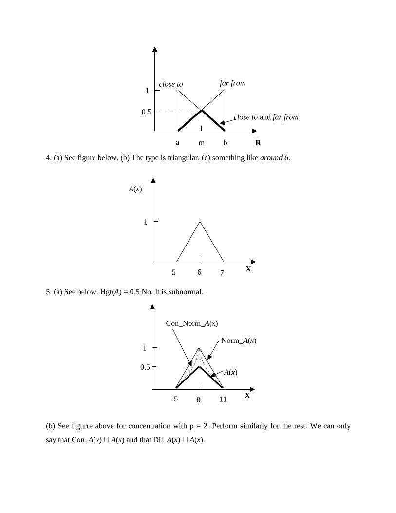
4. (a) See figure below. (b) The type is triangular. (c) something like around 6.
5. (a) See below. Hgt(A) = 0.5 No. It is subnormal.
(b) See figurre above for concentration with p = 2. Perform similarly for the rest. We can only
say that Con_A(x) ⊂ A(x) and that Dil_A(x) ⊃ A(x).
m a b
1
0.5
close to far from
R
close to and far from
1
A(x)
X 5 6 7
1
A(x)
X 5 8 11
0.5
Norm_A(x)
Con_Norm_A(x)

6. It is easy to verify that S(A,B) = Card(A∩B)/Card(A). Therefore, in general S(A,B) ≠ S(B,A).
Clearly they are equal only if Card(A) = Card(B). Note that,
=
+=
+−= ∑ ∑∑ ∑ ∑< ≥∈ ≥ ≥ )()( )()()()( )()(
)()()(Card
1)()()(
)(Card
1),(
xBxA xBxAx xBxA xBxA
xBxAA
xBxAxAA
BASX
= )(Card
)(Card)](),(min[
)(Card
1
A
BAxBxA
Ax
∩=
∑∈X
.
7. A0.1 = {1,2,3,4}; A0.5 = {1,2,3}; A0.8 = {1,2}; A1 = {1}. Clearly, we have
18.05.01.0 0.18.05.01.0 AAAAA ∪∪∪= .
8.By definition we have B = 0.2/2+0.1/5
9. Solve the differential equation!
10. Difficult to depict! We can think abstractly only. See comments in the last paragraph of
section 1.9.2, page 28.
1 2 3 4
5
1
1
1
A
B
X
Y f
3

CHAPTER 2
Fuzzy Set Operations
1. See figure below for an example. It would be interesting to solve this problem using a
computer program with a graphical output. This would start reader to gain skills and insights
about representations of fuzzy sets in a programming language, and about operations.
2. Recall that the drastic product and the drastic sum are t11 and s11, respectively:
==
=otherwise 0
1 if
1 if
t11 xy
yx
yx
==
=otherwise 1
0 if
0 if
s11 xy
yx
yx
Clearly, x t11 (1-x) = 0 and x s11 (1-x) = 1. Thus, A∩ A = φ and A ∪ A = X
3. (a) Note that ).,min(1
1,
1
1min
],max[1
],max[1),max( yx
y
y
x
x
yx
yxyx =
λ+−
λ+−=
λ+−= For (b) proceed the
analogously.
4. First note that ρ(x,y,..,z) continous and increasing assure that S_sum(x,y,..z) also is continous
and monotonic increasing. Comutativity requires that ρ(x,y,..,z) be symmetric under its arguments
2 1 3
1
0.5
B
A
X
A ∪ B
4 5
A ∩ B
interchange. It remains to show that ρ(x,y,..,z) is auto-dual and satisfies the boundary conditions.
That is:
(a) 1 – S_sum(1-x, 1-y,..,1-z) = 1 – {ρ(1-x, 1-y,..,1-z)/[ ρ(x,y,..,z) + ρ(1-x, 1-y,..,1-z)]} =
= S_sum (x,y,…,z).
(b) S_sum(0,…,0) = {ρ(0, 0,..,0)/[ ρ(0,0,..,0) + ρ(1, 1,..,1)]} = 0
S_sum(1,…,1) = {ρ(1, 1,..,1)/[ ρ(1,1,..,1) + ρ(0, 0,..,0)]} = 1.
Symmetric sum is discussed in detail by W. Silvert in Symmetric summation: a class of
operations on fuzzy sets. IEEE Trans. on SMC 9, 657-659, 1979, and by D. Dubois and H. Prade
in A review of fuzzy set aggregation connectives. Information Sciences, 36, 85-121, 1985.
5. Let a = min(x1, x2, .., xn) and b = max(x1, x2, .., xn). A is an aggregation operator and therefore it
is monotonic increasing. Assuming A idempotent, we have:
a = A(a, a,….,a) ≤ A(x1, x2, .., xn) ≤ A(b, b, …, b) = b
Conversely, if we assume min(x1, x2, .., xn) ≤ A(x1, x2, .., xn) ≤ max(x1, x2, .., xn), then
a = min(a, a,….,a) ≤ A(a, a,….,a) ≤ max(a, a,….,a) = a.
Thus, all aggregation operations between the min and max are idempotent, and conversely the
functions A that satifies the inequalities above are the only aggregation operations that are
idempotent. Examples include the averaging operations.
6. The k-th largest element of {x1, x2, …., xn}.
7. Hamming: d(A,B) = 0.1 + 0.2 + 0.4 + 0.8 + 0.1 + 0.8 + 0.4 + 0.2 = 3
Euclidean: d(A,B) = 70,1 =1,3038
Tchebyschev: d(A,B) = 0.8
Poss(A,B) = max [0, 0, 0.1, 0.2, 0.4, 0.2, 0, 0, 0, 0] = 0.4
Nec(A,B) = min [1, 1, 0.9, 0.8, 0.5, 0.2, 0.6, 0.8, 1, 1] = 0.2

9. C(A,B) = ½{ Poss(A,B) + 1 – Poss(A , B)}
C(A ,B) = ½{ Poss(A ,B) + 1 – Poss(A, B)}
Adding the two terms we get C(A, B) + C(A ,B) = ½ .
10. A ⊆ B ⇒ Π(A) ≤ Π(B).
11. Comp(X, A) (u) = 1, ∀u∈[0,1]. See illustration below.
Comp(X,A)
X
A
1,0
u
CHAPTER 3
Information-Based Characterization of Fuzzy
Sets
1. Assume decoding based on modal values. Thus we have:
∑
∑
=
=− =n
ii
n
iii
xA
axA
xF
1
11
)(
)(
)( . We may formulate the optimization problem as follows:
],....,[ where),(min 1 na
aaaaQ = and ∑
=∑=
∑==
N
kkx
kxiA
iakxiA
Qn
i
n
i
1
2
-
1
1
)(
)(
. Computing the derivative of Q
with respect to ai we get the i-th component of the gradient vector:
∑∑
=
=∑=
∑==
∂∂
n
iki
kiN
kixA
xAkx
kxiA
akxiA
a
Q
n
i
n
ii
1
1 )(
)(
)(
)(
2 -
1
1 and we may proceed using any appropriate gradient-
based optimization procedure to determine the ai’s. Alternatively, if we use membership
functions, e.g. as in the CoG method, we have, assuming a discrete universe:
∑
∑==
)(
)(
ˆ 1
m
m
M
mm
xA
xxA
x , where M is the number of discrete intervals and U )( iiAA λ∧= ,

),(Poss XAii =λ . Assuming further a parameterized membership function, e.g. ),,;( cbaxAi , we
note that )))]}(),,,;(max(min(),,,;(max{min[)( xXcbaxAcbaxAxA ii= . Therefore, the expression of Q
and its gradients with respect to the parameters of the membership functions becomes more
complex. This case is much less transparent then the previous.
2. In case (a), we can compute the upper and lower bounds of decoding similarly as suggested in
the figure 3.9 (a). This is illustrated below for Ai. The idea is the same for the remaining Aj’s. The
overall bounds may be found by intersecting the individual bounds.
For the case (b) note that, as shown below, we may get Poss(Ak,X) = 1 and Nec(Ak,X) = 0 for all
k.
encoding
Ai Aj X
Poss(Aj, X) Poss(Ai, X)
-5 5
Nec(Ai, X) Nec(Aj, X)
-5 5
Ai
X’i X’’
i
decoding
Aj
X
-5 5
encoding Poss(Ak,X)=1
Nec(Ak,X)=0
Ai

Case (c) is similar as case (b).
3. Choose appropriate functions to characterize entropy and energy (e.g., piecewise linear and
linear, respectively; see pages 62 and 64) and use equations (3.3) and (3.4). This problem is an
interesting computational exercise for those interested in image analysis.
4. First, note that ∑=
−=n
iiiin ppwppH
121 log),...,( , assuming iii ppw 2log/−= and recalling that
∑=
=n
iip
1
1, we find the maximum of H(.) as follows (p = [p1,…,pn]):
]1[2
),(11∑∑
==
−λ+=λn
ii
n
i
pippL . Computing the derivative of L(.,.) with respect to pi’s we get
02 =λ−=∂∂
ii
pp
L and thus pi = λ/2, i = 1,..,n.
In the general case, we have that, at the maximum )log(loglog(log 2222 jjii pewpew +=+ .
5. One may formulate the following optimization problem for this purpose:
2
1
*
);(
);(),(min ∑
∫∫
=
−=n
ii
p dxpxA
xdxpxAbpxQ . Note that the parameters p should be constrained to within the
underlying universes of discourse.
Aj
X’ =
-5 5
decoding
Ai

CHAPTER 4
Fuzzy Relations and Their Calculus
1. We may find the similarities between patterns by computing a composition between the given
matrix and its transpose. Assuming max-min composition we get the relation S in matrix
form:
=
4.03.03.04.03.0
3.00.11.01.03.0
3.01.09.01.06.0
4.01.01.08.01.0
3.03.06.01.06.0
S .
Clearly S is not reflexive, is symmetric, and is not max-min transitive.
2. We perform the max-min composition. For any t-norm, we may proceed operating with the
relations in matrix form just as we do with standard matrix multiplication, but exchanging the
role of the algebraic product by the chosen t-norm and the role of summation by the max
operation.
=
=6.019.09.03.06.0
4.0119.03.04.0
9.0119.03.09.0
0.10.10000.1
00.19.06.03.00
4.00.10.19.01.01.0
0.16.07.01.03.09.0
4.00.19.06.0
1.02.00.14.0
9.07.00.15.0
oo GR
3. )]}.,(1[s),(1{[inf1)]},(1[s)],(1[1{sup)],(t),([sup yzWzxGyzWzxGyzWzxGzzz
−−−=−−−= Similarly,
)]},(1[t),(1{[sup1)]},(1[t)],(1[1inf{)],(s),([inf yzWzxGyzWzxGyzWzxGzzz
−−−=−−−=
4. We will solve for max-min composition. We perform similarly for other t- and s-norms.

=
1111
1.03.07.05.0
1.03.011
1.03.011
1.03.07.05.0
),(1 yxR ,
=
1111
01.011
01.0031
01.03.01
0111
),(2 yxR ,
=
1111
1.03.07.05.0
1.03.011
1.00311
1.03.07.05.0
),(3 yxR
Thus R = ∩ Rk, k=1,2,3, that is
=
1111
01.07.05.0
01.03.01
01.03.01
03.07.05.0
),( yxR
5. The image is a two dimensional fuzzy relation defined in two finite spaces (universes). The
lighter the pixel (defined by x-y coordinates), the higher the corresponding membership value of
this relation. Similarly, lower membership values correspond to darker pixels of the image.
(a) By applying the operations of contrast intensification and dilation, we affect the image by
either eliminating a gray scale of the values (intensification) or enhancing this range (dilation).
By performing these operations in an iterative fashion, we make this effect more profound and
visible.
(b) This is a design problem which may involve some optimization mechanisms. In a simple
scenario, we can envision the input fuzzy sets to be specified as sets (intervals), see figure below.
They play a role of “filters” compressing the original image. The broader the filter, the higher the
compression rate yet lower quality of the reproduced image (fuzzy relation). In general, if we go
for the max-min composition, we end up with the reconstructed fuzzy relation that subsumes
(includes) the original image.

R
sampling strips (sets)
6. This problem requires the use of the fuzzy set-fuzzy relation composition with x specified as
an empty set or the entire space.
7. The discussed system is governed by the expression RG)](CB)[(AD ••××= . It involves
two unknown fuzzy relations (R and G). Because of that, we have to confine ourselves to
numeric optimization techniques such as gradient-based methods. The ensuing problem reads as:
RG)](CB)[(ADmin ••××−
with respect to R and G for A, B, and C given, where stands for a distance function
(Euclidean, Hamming, etc.).
8. The problem induces the following expression ])y,)tR(x(x[Ag lkki
mn,
lk,ij ∨= where G = [gij].
The reconstruction problem requires a determination of R for A, B, and G provided. For the
given t-norm we obtain the solution of the form
]g)(y)tB(x[A)y,R(x ijljki
pc,
ji,lk ϕ= ∧ .
9. The relationship country-currency establishes a Boolean relation each country uses (officially)
its own currency. The remaining relations are clearly fuzzy.
CHAPTER 5
Fuzzy Numbers
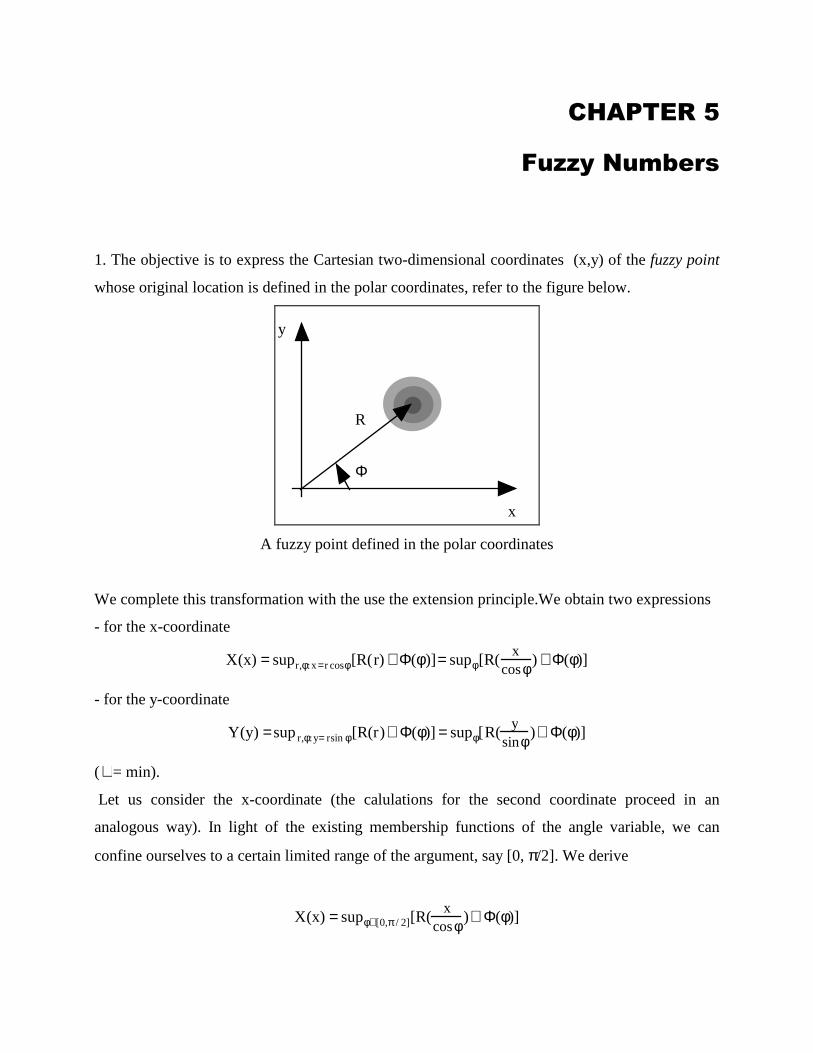
1. The objective is to express the Cartesian two-dimensional coordinates (x,y) of the fuzzy point
whose original location is defined in the polar coordinates, refer to the figure below.
x
y
R
Φ
A fuzzy point defined in the polar coordinates
We complete this transformation with the use the extension principle.We obtain two expressions
- for the x-coordinate
X(x) = supr,φ:x=r cosφ[R(r) ∧ Φ(φ)] = supφ[R(x
cosφ ) ∧ Φ(φ)]
- for the y-coordinate
Y(y) =supr,φ:y= rsinφ[R(r)∧ Φ(φ)] = supφ[R(y
sinφ )∧ Φ(φ)]
(∧= min).
Let us consider the x-coordinate (the calulations for the second coordinate proceed in an
analogous way). In light of the existing membership functions of the angle variable, we can
confine ourselves to a certain limited range of the argument, say [0, π/2]. We derive
X(x) = supφ∈[0,π / 2][R(x
cosφ )∧ Φ(φ)]

The equivalent optimization problem implies a nonlinear equation to be solved with respect to
the angle variable for the value of x being fixed
R(x
cosφ) = Φ(φ)
(1)
that is
exp[−(x
cosφ −1)2 ] = exp[−(φ − π / 3)2]
We look for the solutions to the above nonlinear equation that fall under the already defined
range of the values of the angle. Considering the arguments of exponential functions we get
xcosφ −1= ±(φ − π / 3)
The solutions can be produced numerically. In the case of multiplicity of the solutions (c), we
pick up the one for which Φ(φ1), Φ(φ2), ..., Φ(φc ) attains maximum. As the solutions depend on
the values of the second variable (x) regarded here as parameter, we construct the membership
function of X by solving (1) for selected values of x and plotting such relationship.
2. The discussed cases embrace the following situations:
- fuzzy velocity; exact time. The resulting distance is the distance represented as a fuzzy number
with the triangular membership function as illustrated below.
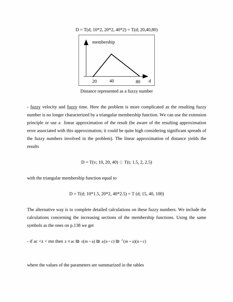
D = T(d; 10*2, 20*2, 40*2) = T(d; 20,40,80)
d20
membership
40 80
Distance represented as a fuzzy number
- fuzzy velocity and fuzzy time. Here the problem is more complicated as the resulting fuzzy
number is no longer characterized by a triangular membership function. We can use the extension
principle or use a linear approximation of the result (be aware of the resulting approximation
error associated with this approximation; it could be quite high considering significant spreads of
the fuzzy numbers involved in the problem). The linear approximation of distance yields the
results
D = T(v; 10, 20, 40) ⊗ T(t; 1.5, 2, 2.5)
with the triangular membership function equal to
D = T(d; 10*1.5, 20*2, 40*2.5) = T (d; 15, 40, 100)
The alternative way is to complete detailed calculations on these fuzzy numbers. We include the
calculations concerning the increasing sections of the membership functions. Using the same
symbols as the ones on p.138 we get
- if ac <z < mn then z = ac+ ωc(m− a)+ ωa(n− c) + ω2(m − a)(n− c)
where the values of the parameters are summarized in the tables

a m b
10 20 40
c n d
1.5 2.0 2.5
The above relationship is just a quadratic equation that needs to be solved with respect to ω
5ω 2 + 20ω + 15− z = 0
The solution (namely, the membership function over z) is given in the form
ω = −2+ 100+ 20z10
(the second root is irrelevant in the framework of this problem). The membership function is
defined over z in the range [15, 40]. Note it is a nonlinear function of z. It coincides with the
linear approximation at the boundaries that is z =15 and z =40.
3. Owing to the triangular form of the membership functions of the fuzzy numbers, the mean is
computed as follows
0.5 *[T(x; 1, 3, 5) + T(x; 2, 4, 6)] = 0.5* T(x; 3, 7, 11) = T (x; 1.5, 3.5, 5.5)
In general for “n” arguments each being equal to T(x; 1, 3, 5) we derive
1n
T(x;1, 3, 5) =i =1
n
∑1n
T(x;n, 3*n, 5* n) =i =1
n
∑ T(x;1, 3, 5)
Note that the result is just the original fuzzy set being used in the entire aggregation process. This
stands in a quite evident contrast with the phenomenon of averaging encountered in statistics.

4. The addition of two fuzzy numbers yields the following membership function of the result
B(b) = supa,x∈R: b= a+x[A(a) ∧ X(x)]
There is no unique solution to this problem. One may, however, rewrite the above expression in
an equivalent format. To do so, let us introduce a fuzzy relation R defined as
R(x, b) = A(b-x)
Then
B(b) = supx∈R[R(x, b) ∧ X(x)]
The above is nothing but a fuzzy relational equation with the sup-min composition
B = A oR
(2)
It has to be solved with respect to X for R and B provided. The maximal solution to (2) comes in
the form
X(x) = inf b∈R[R(x,b)→ X(x)] = inf b∈R
1 if R(x,b)≤ X(x)
X(x) if R(x,b) > X(x)
5. The solution to the system of two equations (and two unknown fuzzy sets X and Y) is handled
in a similar way as outlined in the previous problem, namely by solving the corresponding system
of fuzzy relational equations. One should elaborate on a way in which this type of transformation
takes place. Consider the first equation in the system of the equations. The membership function
of B1 results directly from the use of the extension principle
B1(b) = supx,y,a1 ,a2 ∈R:a1x+ a2y= b[X(x)∧ Y(y) ∧A11(a1)∧ A12(a2)]
We transform this expression through a number of steps:
- firstly, define two fuzzy relations
A ~(a1,a2 ) = A11(a1)∧ A12(a2)
X ~(x,y) = X(x) ∧Y(y)
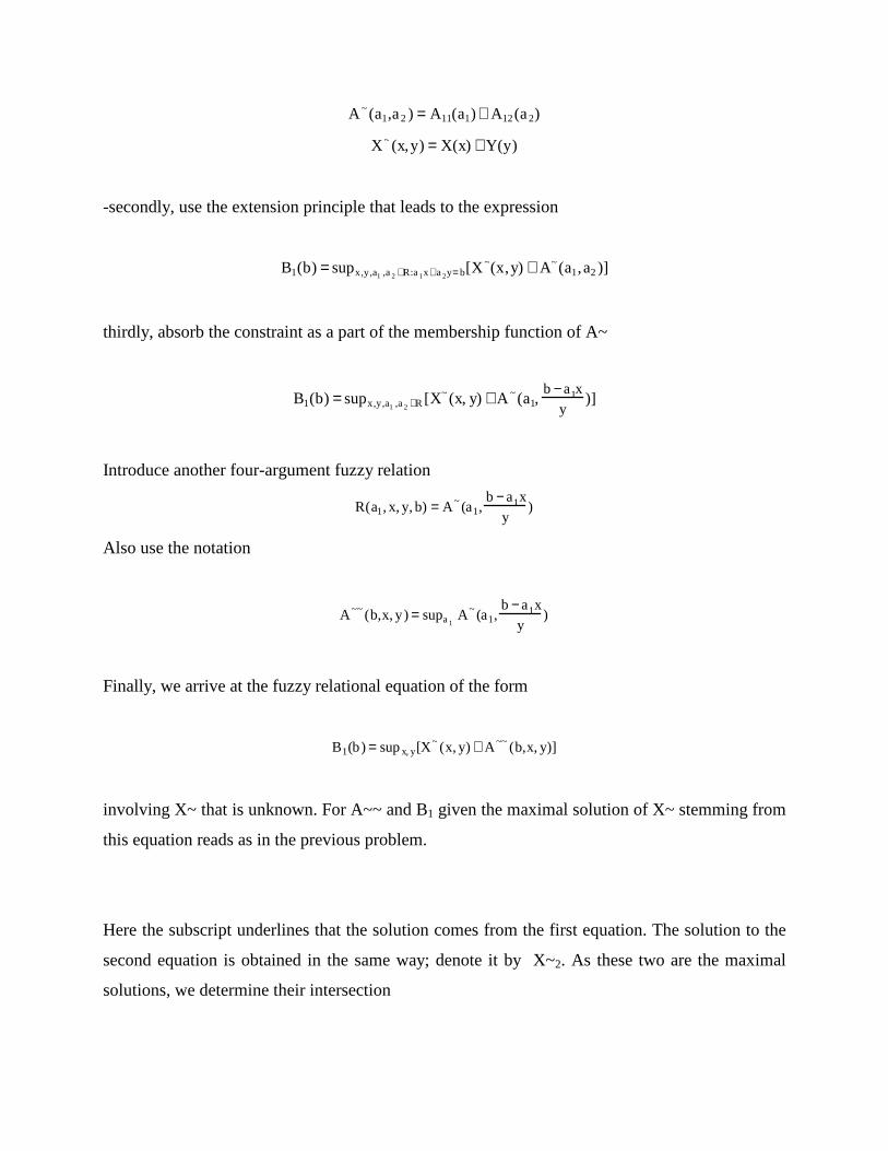
-secondly, use the extension principle that leads to the expression
B1(b) = supx,y,a1 ,a2 ∈R:a1x+ a2y= b[X~(x,y) ∧ A~(a1,a2)]
thirdly, absorb the constraint as a part of the membership function of A~
B1(b) = supx,y,a1 ,a2 ∈R [X~(x, y) ∧A ~(a1,b − a1x
y)]
Introduce another four-argument fuzzy relation
R(a1, x, y, b)= A ~(a1,b − a1x
y)
Also use the notation
A ~~(b,x, y)= supa1A ~(a1,
b − a1x
y)
Finally, we arrive at the fuzzy relational equation of the form
B1(b)= supx, y[X~(x, y) ∧ A ~~(b,x, y)]
involving X~ that is unknown. For A~~ and B1 given the maximal solution of X~ stemming from
this equation reads as in the previous problem.
Here the subscript underlines that the solution comes from the first equation. The solution to the
second equation is obtained in the same way; denote it by X~2. As these two are the maximal
solutions, we determine their intersection

X~= X~1 ∩ X~2
Note that X~ is a fuzzy relation defined in X Y. To obtain the individual fuzzy sets we project
X~ on the corresponding universes, that is
- projection on X returns the fuzzy set with the membership function equal to
supy∈R X ~ (x,y)
- projection on Y gives rise to the expression
supx∈R X ~ (x,y)
The discussed method easily generalizes to a system of equations with “n” variables (fuzzy sets).
6. The problem requires the use of the extension principle and the solutions are obtained very
much in the same way as discussed in detail in the first problem.
7 and 8 refer to problem 1.
9. The process of subtracting A from a numeric value is very much simplified because of the use
of the triangular membership function of A. We have
A=(0.8, 1.0, 1.2), B = {10}. Note also that -A = (-1.2, -1, -0.8)
First we obtain
B1 = B - A = B +(-A) = {10} + (-1.2, -1, -0.8)= (10, 10, 10) - (-1.2, -1, -0.8)= (8.8, 9.0,9.2). The
support of B1, supp(B1), is equal to 9.2-8.8 = 0.4
The second iteration yields
B2 = B1 - A = B1 +(-A) = (8.8, 9.0, 9.2) + (-1.2, -1, -0.8)= (7.6, 8.0, 8.4), supp(B2) = 0.8
Performing successive iterations we obtain
B3 = B2 - A = B2 +(-A) = (7.6, 8.0, 8.4) + (-1.2, -1, -0.8)= (6.4, 7.0, 7.6)), supp(B3) = 1.2
B4 = B3 - A = B3 +(-A) = (6.4, 7.0, 7.6) + (-1.2, -1, -0.8)= (5.2, 6.0, 6.8), supp(B4) = 1.6

B5 = B4 - A = B4 +(-A) = (5.2, 6.0, 6.8) + (-1.2, -1, -0.8)= (4.0, 5.0, 6.0), supp(B5) = 2.0
...
Evidently, the results become fuzzier, namely the supports of the successive fuzzy sets become
larger. This is an inherent phenomenon occurring in fuzzy arithmetic. It also suggests using
relatively short chains of computing (not too many iterations) in order to avoid an excessively
high (unacceptable) level of accumulation of fuzziness.
10 The use of the extension principle leads to the expression
Y(y) =supx∈R:4x(1− x)= y[A(x)]
As both the mapping as well as the membership function are symmetrical, the two roots of the
equation with respect to x
4x(1-x) =y
produce the same result in terms of the resulting membership values, A(x1)=A(x2). The
nonlinear membership function has its support between 0.99 and 1.00; see figure below.
x
y
f(x)
A
f(A)
First iteration of the triangular fuzzy number through a quadratic map

CHAPTER 6
Fuzzy Sets and Probability
1. In this example the fuzzy set is reduced to a set. The location of A and the probability density
function (pdf) p(x) is illustrated in the figure below.
0 c
p(x)
a b x
A1.0
A distribution of A and the pdf p(x)
The calculations of the probability of A, Prob(A), its expected value E(A), and the variance V(A)
are realized following the formulas
Pr ob(A)= A(x)p(x)dx = p(x)dx = c − ac
a
c
∫0
b
∫
E(A) = xA(x)p(x)dx = 1c
xdx = c2 − a2
2ca
c
∫0
b
∫
Var(A) = (x − E(A(x))2p(x)dx= 1c
(x − c2 − a2
2ca
c
∫0
b
∫ )2dx =
= c3 − a3
3c− (c2 − a2)2
2c2 + (c2 − a2)2(c − a)4c3
The computations for the second case envisioned in the problem are completed in the same way.
2. We encounter a problem of a sensor affected by a random noise. The general scenario of this
nature is commonly encountered in control, communications, etc. The main difference lies here

in the fact of two distinct forms of information granules, namely fuzziness and randomness. To
start with any computations, it becomes indispensable to transform the probabilistic facet of
uncertainty into its fuzzy set counterpart. As we encounter continuous pdf, we first discretize it
and convert into the membership function (see formula 6.10). Second, we complete addition of
the two fuzzy quantities, say C = A ⊕ B. The overall process of transformation is portrayed in
the figure below.
C
p(z)
+A
B
+A
probability-possibility transformation
Computing fuzzy output of the sensor affected by an additive noise
Alternatively, we transform the fuzzy reading of the sensor into the probability function. Owing
to the additive nature of the noise, these two random variables are afterwards added giving rise to
the probability function D. Finally, the probability of the fuzzy event C is computed in the usual
form
Pr ob(C)= C(x)pD (x)dx∫
where pD denotes the pdf of D.
3. This is a design problem that requires some numeric optimization. The choice of the form of
the four linguistic labels (fuzzy sets) is very much open. We confine ourselves to triangular or
trapezoidal membership functions. This choice simplifies a lot a way in which these fuzzy sets
can be distributed along the universe of discourse. The modifications (e.g., expansion or
contraction of the membership function) are performed by equalizing of the respective fuzzy
sets. This means that we request that each fuzzy set embraces the same fraction of the
experimental data. More specifically, we are concerned about the s-count of the fuzzy set as
different elements of the data set may belong to different degrees of membership. Let us
concentrate on the fuzzy sets shown below.

A1 A2 A3 A4
xmin a1 a2 a3 a4 max
Equalization of fuzzy sets
Put c=1/8. The equalization process can be sketched as follows
- scan the current argument (x) starting from min and determine a1 for which the cumulative
probability
A(xk )k:A(x k )<a1
∑ ≤ c
is equal “c”. Repeat the same process for the successive fuzzy sets starting respectively from a1
(for A2) and moving toward higher values of the argument.
In general, the higher the concentration of data, the more narrow the fuzzy set constructed over
this particular region. Once the fuzzy sets have been already determined, we can easily determine
their expected value and variance.
CHAPTER 7
Linguistic Variables
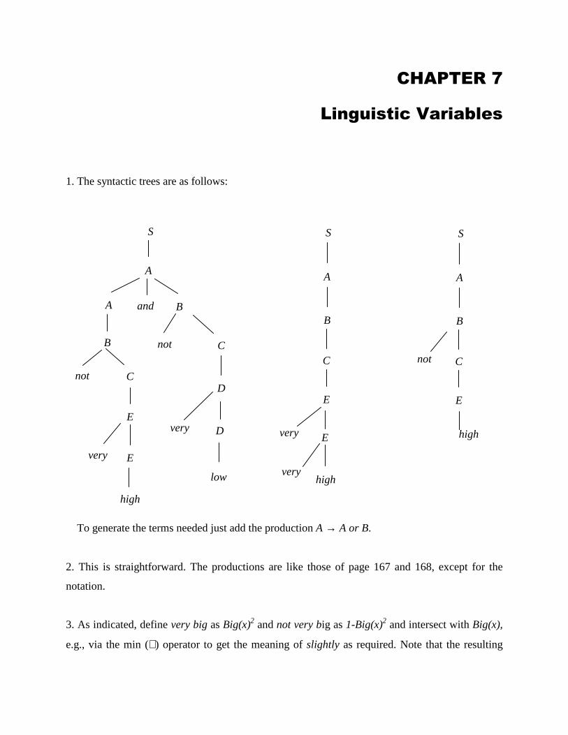
1. The syntactic trees are as follows:
To generate the terms needed just add the production A → A or B.
2. This is straightforward. The productions are like those of page 167 and 168, except for the
notation.
3. As indicated, define very big as Big(x)2 and not very big as 1-Big(x)2 and intersect with Big(x),
e.g., via the min (∧) operator to get the meaning of slightly as required. Note that the resulting
S
A
A B and
not C
C B
E
not
E very
high
D
low
very D
S
A
B
C
E
very E
very high
S
A
B
C
E
not
high
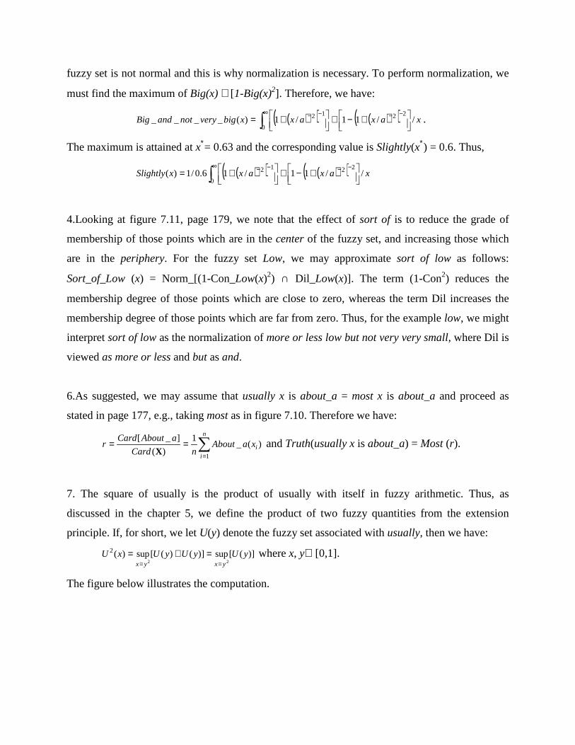
fuzzy set is not normal and this is why normalization is necessary. To perform normalization, we
must find the maximum of Big(x) ∧ [1-Big(x)2]. Therefore, we have:
( )( ) ( )( ) xaxaxxbigverynotandBig //11/1)(____22
0
12
+−∧
+=
−−∞ −−∫ .
The maximum is attained at x∗= 0.63 and the corresponding value is Slightly(x∗) = 0.6. Thus,
( )( ) ( )( ) xaxaxxSlightly //11/16.0/1)(22
0
12
+−∧
+=
−−∞ −−∫
4.Looking at figure 7.11, page 179, we note that the effect of sort of is to reduce the grade of
membership of those points which are in the center of the fuzzy set, and increasing those which
are in the periphery. For the fuzzy set Low, we may approximate sort of low as follows:
Sort_of_Low (x) = Norm_[(1-Con_Low(x)2) ∩ Dil_Low(x)]. The term (1-Con2) reduces the
membership degree of those points which are close to zero, whereas the term Dil increases the
membership degree of those points which are far from zero. Thus, for the example low, we might
interpret sort of low as the normalization of more or less low but not very very small, where Dil is
viewed as more or less and but as and.
6.As suggested, we may assume that usually x is about_a = most x is about_a and proceed as
stated in page 177, e.g., taking most as in figure 7.10. Therefore we have:
∑=
==n
iixaAbout
nCard
aAboutCardr
1
)(_1
)(
]_[
X and Truth(usually x is about_a) = Most (r).
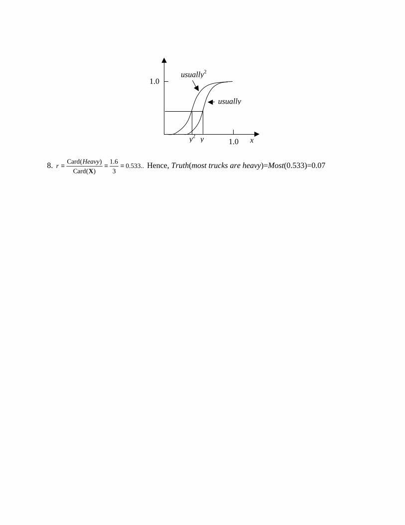
7. The square of usually is the product of usually with itself in fuzzy arithmetic. Thus, as
discussed in the chapter 5, we define the product of two fuzzy quantities from the extension
principle. If, for short, we let U(y) denote the fuzzy set associated with usually, then we have:
)]([sup)]()([sup)(22
2 yUyUyUxUyxyx ==
=∧= where x, y∈ [0,1].
The figure below illustrates the computation.
8. ..533.03
6.1
)(Card
)(Card ===X
Heavyr Hence, Truth(most trucks are heavy)=Most(0.533)=0.07
1.0
1.0 y y2
usually
usually2
x
CHAPTER 8
Fuzzy Logic
1. From the formulation of the problem, we get false(v) =τ(1-A(x))(v) Assume a model of
linguistic truth to be linear, namely τ(v) = v defined in the unit interval. Then the following
interpretation holds
(X is A) is false = B
with
B(x) =1-A(x)
for any x defined in X.
2. The discussed linguistic modifiers yield the expressions
(X is A) is very true = B; B(x) = A2(x)
(X is A) is very false = C; C(x) = (1-A(x))2
3. The linguistic truth of the expression
τ(A and B)
is given in the form
τA and B(v) = supv=wtz[min(τA (w),τ A (w))]
Because of the discrete format of the universe of discourse, the calculations are carried out for
their successive entries. Put, as an example, v=0. The calculations of τ(A and B) for this
particular value of the argument imply a series of pairs of values of w and z:
w=0, z=0; w=0, z =0.1; w=0, z=0.2; ..., w=0, z=1;
w=0.1, z=0; w=0.2, z=0; ...., w =1, z =0.
By taking the minimum of the corresponding membership values (t-norm: minimum) we obtain
the membership of the truth value equal to 1.

When proceeding with some other interactive t-norms such as product, the results are distributed
non uniformly across the universe of discourse. Say, if w=0.7 and z=0.8 then
v = w*z =0.56.
4. We follow the basic formula supporting calculations of linguistic truth
τ i = supx i :v=A i (x ) A(x)
Because A(x) ∈ {0, 1} the resulting linguistic truth assumes only two values (either 0 or 1). The
set format of A simplifies all computations. Refer to the figure below. Take x ∉ [a, b] or
equivalently consider v lying outside the region [a, b]. In this particular range, the truth value is
equal to 0. Subsequently for x ∈ [a, b] (that is an equivalent representation of v ∈ [a, b]) the truth
value is equal to 1.
membership
Ai A
a b x d e
α
β
Computations of linguistic truth for A and Ai
5. The form of the input implies the fuzzy truth of the form
τi(v) =
1 if v = 0.50, otherwise
Assuming that the rule is true, meaning that
τR i(v) = v

we obtain the fuzzy truth of the conclusion in the form of a linear function, see figure below.
τBi
v1.0
0.5
Fuzzy truth value of the conclusion
Finally, the inverse truth qualification leads to the fuzzy set B
B(z)=0.5 if Bi (z) < 0.5B i (z) otherwise
We compare this style of inference with two other commonly encountered models:
(a) associative memories using Hebbian learning. The fuzzy relation R is taken as a Cartesian
product of Ai and Bi. Then the max-min composition of fuzzy singleton A and R produces an
outcome of the reasoning mechanism
(b) fuzzy relational-equation approach computes R as an implication (being more specific,
Godelian implication) of Ai and Bi. The max-min composition is utilized afterwards.
As an example, let us use two fuzzy sets Ai and Bi
Ai = [1.0 0.7 0.5 0.2]
Bi = [0.3 0.8 1.0 0.6]
Using the first method, the fuzzy relation R is equal to

R =
0.3 0.8 1.0 0.60.3 0.7 0.7 0.60.3 0.5 0.5 0.50.2 0.2 0.2 0.2
and the conclusion arises as a fuzzy set
B = [0.3 0.5 0.5 0.5]
The second approach leads to the fuzzy relation
R =
0.3 0.8 1.0 0.60.3 1.0 1.0 0.60.3 1.0 1.0 0.51.0 1.0 1.0 1.0
and, subsequently, the result of the form [0.3 1.0 1.0 1.0]
The fuzzy logic approach leads to the expression
B = [0.5 0.8 1.0 0.6]
This simple example reveals that these results can be arranged in the form of two inclusions
[0.3 0.5 0.5 0.5] < [0.5 0.8 1.0 0.6]
and
[0.3 0.5 0.5 0.5] < [0.3 1.0 1.0 1.0]

CHAPTER 9
Fuzzy Measures and Fuzzy Integrals
1. The λ-measure is computed following formula (9.5) provided on p. 208 of the book. We
solve the associated polynomial equation with respect to λ. The roots are:
6.56478, -3.14579-2.94849 i, 3.14579+2.94849 i, -0.945946, and 0.
The corresponding value of the normalization factor used in the fuzzy measure is taken as -
0.945946. In the sequel we determine the relevance of information produced by any pair of
sensors. Overall, we have
52
= 5!
2!3!= 10
pairs of the sensors. The results of successive computations of the fuzzy measure of the pairs of
the sensors are summarized in the tabular format
sensor no. fuzzy measure
1, 2 0.767568
1, 3 0.645946
1, 4 0.443243
1, 5 0.564865
2, 3 0.885811
2, 4 0.801351
2, 5 0.852027
3, 4 0.693919
3, 5 0.765878
4, 5 0.622297
Next we repeat computations for each triple of the sensors. Here we get
53
=
5!3!2!
= 10
possible arrangements of the sensors. Again, the results are collected in the following table
(additionally, indicated is the combination of the sensors producing the highest value of the fuzzy
measure)
sensors fuzzy measure
1, 2, 3 0.918225
1, 2, 4 0.849744
1, 2,5 0.890833
2, 3, 4 0.934432
2, 3, 5 0.958743
3, 4, 1 0.762637
3, 4, 5 0.848534
4, 1, 5 0.704565
4, 2, 5 0.934432
5, 1, 3 0.820982
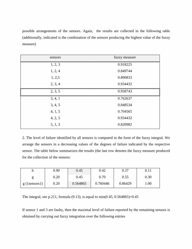
2. The level of failure identified by all sensors is computed in the form of the fuzzy integral. We
arrange the sensors in a decreasing values of the degrees of failure indicated by the respective
sensor. The table below summarizes the results (the last row denotes the fuzzy measure produced
for the collection of the sensors:
h 0.90 0.45 0.42 0.37 0.11
g 0.20 0.45 0.70 0.55 0.30
g ({sensors}) 0.20 0.564865 0.760446 0.86429 1.00
The integral, see p.211, formula (9.13), is equal to min(0.45, 0.564865)=0.45
If sensor 1 and 3 are faulty, then the maximal level of failure reported by the remaining sensors is
obtained by carrying out fuzzy integration over the following entries

h 0.45 0.42 0.11
g 0.45 0.70 0.30
g ({sensors}) 0.45 0.852027 0.910236
The result is equal to 0.45. This points out that the level of identified fault (even though some
sensors were inactive) has not been changed.
3. Here we sketch the solution by focusing on the underlying idea. The relevance of the classifier
with respect to a given class is meant to be its accuracy; the closer this number to 1, the better.
We construct a fuzzy measure over the family of the classifiers; subsequently we compute the
fuzzy integral over the corresponding columns to obtain final class membership values. See
figure below.
classi
classifier1
classifier2
classifier4
fuzzy measure
class assignment
fuzzy integral= class membership in class “i”
Computations of the fuzzy measure and fuzzy integrals for the individual classes in the
classification problem

4. The pieces of the image are tagged (subjectively) by some values of the fuzzy measure. This
assignment is subjective: the higher the relevance of the piece, the higher the relevance, figure
below. For instance, if we anticipate that a certain piece is essential for understanding (or
envisioning) the entire image then we attach to it a high value of the fuzzy measure. On the other
hand, if some other fragment of the image does not seem to be essential then the associated value
of the fuzzy measure is made low. One of the possibilities of such allocation of the fuzzy measure
is shown below. As a matter of fact, this reflects our intuitive insight as to the entire image,
especially once it becomes reconstructed from these pieces. For the assigned values of the fuzzy
measure the roots of the polynomial equation are given as: -7.07236, -3.53154-3.15859i, -
3.53154+3.15859 i, -0.959798, 0 and thus the parameter used for further computations of the
fuzzy measure is equal to -0.959798.
0.75 0.30
0.70
0.25
0.20
. Elements of an image under analysis
5. First we compute the value of the λ - parameter of the fuzzy measure for the values of gi’s
equal to 0.05, 0.40, 0.10, 0.60, 0.40, 0.55 (note that there is an error in the dimension of the
vector; let us make the number of sources equal to 5). Solving the resulting polynomial equation,
the solution of interest is -0.773061. Let us now compute the values of the fuzzy integral for the
respective fuzzy sets; the results are included in the tables below

h 0.50 0.30 0.20 0.00 0.00
g 0.05 0.10 0.40 0.60 0.40
g ({elements}) 0.05 0.146135 0.500946 0.868589 1.00
h 0.70 0.50 0.40 0.20 0.10
g 0.40 0.05 0.10 0.60 0.40
g ({elements}) 0.40 0.434539 0.500946 0.868589 1.00
h 0.70 0.40 0.30 0.20 0.00
g 0.40 0.10 0.60 0.05 0.40
g ({elements}) 0.40 0.469078 0.851502 0.868589 1.00
Finally, let us compare the results of the these computations with the experimental results
fuzzy integral (computed) fuzzy integral (target value)
0.20 0.87
0.50 0.52
0.40 0.13
The differences are significant. As a transformation, we can think of some linguistic modifiers
applied to the fuzzy set (h) under integration. Another option would be to consider a complement
of h.
CHAPTER 10
Rule-Based Computations
1. For each x∈X, let B(x) = [µ ∧ A(x)] + (1- µ). If µ ≥ A(x) then B(x) = A(x) + (1- µ). Thus B(x)
≥ A(x). If µ ≤ A(x) then B(x) = 1 ≥ A(x). Therefore B(x) ≥ A(x) for each x∈X which means that
S(A) ≥ S(B).
Next, we can say that, if A1 = A2, then S(B1) ≥ S(B2) because if B1(x) = [µ1∧A(x)] + (1- µ1) and
B2(x) = [µ2∧ A(x)] + (1- µ2) there are three possibilities:
a) A(x) ≤ µ2 ≤ µ1 . Then B1(x) = A(x) + (1- µ1) and B2(x) = A(x) + (1- µ2). Since µ2 ≤ µ1 we have
(1-µ1) ≤ (1-µ2) and hence B2 (x) ≥ B1(x).
b) µ2 ≤ A(x) ≤ µ1. Then B1(x) = A(x) + (1- µ1) and B2(x) = µ2 + (1- µ2) = 1 ≥ B1(x).
c) µ1 ≤ µ2 ≤ A(x). Then B1(x) = µ1 + (1- µ1) =1 and B2(x) = µ2 + (1- µ2) = 1 ≥ B1(x).
We can conclude that B2 (x) ≥ B1(x) ∀ x ∈ X. Therefore S(B1) ≥ S(B2).
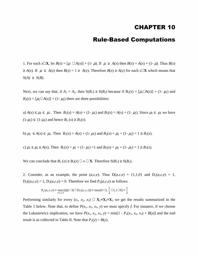
2. Consider, as an example, the point (a,c,e). Thus D(a,c,e) = {1,1,0} and D1(a,c,e) = 1,
D2((a,c,e) = 1, D3(a,c,e) = 0. Therefore we find Pa(a,c,e) as follows
2
1]01 ,1
2
1 ,10max[)],,()3/([max),,(
3,2,1=∧∧∧=∧=
=ecaDiQecaP i
ia
Performing similarly for every (x1, x2, x3) ∈ X1×X2×X3 we get the results summarized in the
Table 1 below. Note that, to define P(x1, x2, x3, y) we must specify f. For instance, if we choose
the Lukasiewicz implication, we have P(x1, x2, x3, y) = min[1 - Pa(x1, x2, x3) + B(y)] and the end
result is as collected in Table II. Note that Pc(y) = B(y).

Table I
x1 x2 x3 A(x1) A(x2) A(x3) d1 d2 d3 Pa
a c e 1 1 0 1 1 0 1/2
a c f 1 1 1 1 1 1 1
a d e 1 0 0 1 0 0 0
a d f 1 0 1 1 1 0 1/2
b c e 0 1 0 1 0 0 0
b c f 0 1 1 1 1 0 1/2
b d e 0 0 0 0 0 0 0
b d f 0 0 1 1 0 0 0
Table II
x1 a a a a a a a a b b b b b b b b
x2 c c c c d d d d c c c c d d d d
x3 e e f f e e f f e e f f e e f f
y g h g h g h g h g h g h g h g h
P 1 1/2 1 0 1 1 1 1/2 1 1 1 1/2 1 1 1 1
3. To prove (a) and (b) two rows of R are of interest, namely, the rows that satisfy
.1)](),(min[ 1)](),(min[ and == rpki zCxAzCxA Let us assume that the first is the (i,k)th row and that
second is the (p,r)th row. since )(1)( zCzC −= it is clear that (i,k) and (p,r) are not equal. We know
that for each j, )( )( thatand yBryBr pjrjijk == ( ijkr and pjrr are the (ijk) and (pjr) elements of C
R
and of CR , respectively), but what about ijkr and pjrr ? In CR we have 0)(1)( =−= kk zCzC
because zk was chosen such that .1)( =kzC Thus min[A(xi), C(zk)] =0. Since 0)( ≥jyB for any j,
due to the Godelian implication 1=ijkr . Hence we have ijkijkijkijk rrrr == ],min[ . Analogously,
pjrpjr rr = . The only interesting row in R is the one for which A(x) = 1. Therefore, the maximum
of all the minima of A(x) and C(z) [resp. )(zC ] and R is equal to )(yB [resp. B(y)].
To prove (c) suppose for some s,t,u A(xs) =1, and C(zu) = B(yt) = 0.5. Then it is easy to check that
1== stustu rr and hence .1=stur In addition, because both min[A(xs), C(zu)] and min[ )](),( us zCxA

are equal to 1, the row (s,u) is different to one of the rows (i,k) and (p,r) mentioned above. Hence,
they are not relevant for the behavior of R with respect to the input A(x) ∧ C(z) or A(x) ∧ )(zC .
But with the input )()( zxA Z∧ it follows that 1)](),(min[ =us zxA Z and hence 1]),(),(min[ =stuus rzxA Z
which means that 1]),(),(min[max)( ,,,
== utsusus
t rzxAyB Z . But this cannot be the case because we
have assumed that 5.0)( =tyB .
4. Just note that, (a) if )()( zCxA < then )()()](),(min[ yBxAzCxA ≤= but it may be the case that
)()( yBzC > and (b) if )()( zCxA > then )()()](),(min[ yBzCyBxA ≤= but it may be the case that
)()( xAyB < . See below.
5. Inferring B’(y) using the composition rule reads as )],( t )('[sup)(' yxRxAyBx
= . But 1),( =yxR if
)()( xAyB ≥ and R(x,y) = 0 otherwise. Therefore, if we let )}()(|{)( xAyBxA yR ≥∈= X we get
)('sup)(')(
uAyByRAu∈
= .
6. Since the rules are conjunctively aggregated we have:
)]()([)]()([),(),(),( 221121 yBxAyBxAyxRyxRyxR ∨∧∨=∧=
Using the compositional rule of inference with t = ∧, and assuming A normal we get
)}()]()([)]()({[sup)( 2211 xAyBxAyBxAyBx
∧∨∧∨= =
)}()])()([)]()([)]()([)]()({([sup 21212121 xAyByBxAyByBxAxAxAx
∧∧∨∧∨∧∨∧= =
)]}()()([)]()()([)]()()([)]()()({[sup 21212121 xAyByBxAxAyBxAyBxAxAxAxAx
∧∧∨∧∧∨∧∧∨∧∧=
)],()()([sup)],()()([sup)],()()([supmax{ 212121 xAxAyBxAyBxAxAxAxAxxx
∧∧∧∧∧∧=
)]}()()([sup 21 xAyByBx
∧∧ . Thus we get
A(x) C(z) B(y) (a)
A(x) B(y) C(z) (b)

)]()([)](),(Poss[)](),(Poss[),(Poss)( 21122121 yByByBAAyBAAAAAyB ∧∨∧∨∧∨∧= .
7. It is instructive to detail the derivation of the necessary conditions for the case shown in page
256 of the textbook because this problem is analogous. Thus, let us first consider the example in
which we have the fact V is D and the rules
If X is A1, then Y is B1
If Y is G2, then W is S2
If X is A3, then W is S3
These four pieces of knowledge conjunct to
)())()(())()(())()((),,( 332211 xDzSxAzSyGyBxAzyxH ∧∨∧∨∧∨= .
Projecting H(x,y,z) on Y we get U is F where
)].()([)](),A[Poss(
)](),(Poss[)],(Poss),(Poss[)]()(),(Poss[
)](),(Poss[)](),(Poss[)],(Poss[)(
3223
312123321
3313131
zSzSzSD
zSBGBGDAzSzSDA
zSDAAzSDADAAyF
∧∨∧
∨∧∨∧∨∧∧
∨∧∩∨∧∨∩=
To
obtain a degree of inconsistency of α, it must be the case that zzF ∀α−≤ ,1)( . Since S2 and S3 are
assumed to be normal fuzzy sets, we must have
α−≤
α−≤
1),(Poss
1),(Poss
2
1
DA
DA
and these conditions guarantee that α≥),(Poss 31 AA . In addition, we must have
zzSzS ∀α−≤∧ ,1)()( 32 , that is α−≤ 1)/(Poss 32 SS . It must also be the case that α−≤ 1),(Poss 12 BG
or, equivalently, α−≥− 1),(Nec1 12 BG what gives another necessary condition for the existence of
potential conflicts relating the values of the linking variable, namely α≥),(Nec 12 BG . Therefore,
there are three necessary conditions to obtain any inconsistency in this case: for some ]1,0(∈α
1- α−≤ 1),(Poss 32 SS
2- α≥),(Poss 31 AA
3- α≥),(Nec 12 BG
Note the pattern of the conditions obtained. The first condition relates the consequent of the last
two rules given, whereas the second relates the values of the same variable appearing in the
antecedent and the last relates the linking variable among rule antecedent and consequent.

Therefore, we could proceed analogously with the rules given in the problem, but it is clear that,
based on the result and the pattern above, we get
1- α−≤ 1),(Poss 22 SC
2- α≥),(Poss 32 AA
3- α≥),(Poss 54 BB
4- α≥),(Nec 12 BB
8. The minimal cover for the new rule introduced is the subset that includes the two rules linked
by variable V6. The corresponding CT-matrix T’ for the subset contains only the second (R2) and
the third (R3) columns of the matrix at the top of page 257. Thus, the test vector for the new rule
is VT = [ 0 -C6 0 0 0 0 -D2 0 0 F2] and applying the matrix composition we get
++++++++++++++++++
=
−
−−−
−−
∗),(Poss00),(Poss000000
00000000),(Poss0
0
00
0
0
00
00
00
0
0
1212
26
1
1
1
21
2
2
FFDD
CC
F
E
D
JJ
C
A
V T
For the fuzzy sets given, we have α≥= 5.0),(Poss 26 CC , α≥= 1),(Poss 12 DD and
α−≤= 12.0),(Poss 12 FF . Next we find, by inspection, that V is the linking variable and, for
example, assuming J1 = {1/1, 0.8/2, 0.7/3} and J2 = {0/1, 0.7/2, 1/3} we get α≥= 7.0),(Nec 21 JJ .
Thus we have an indicator that a potential conflict exists with the insertion of the new rule.

CHAPTER 11
Fuzzy Neurocomputation
1. This is a small simulation project. The network can be realized and experimented with using
MATLAB, MATHEMATICA as well as any other simulation package. The main task is to write
down the expressions governing the behavior of the network based on the structure of the
network and including in this description the specific forms of the triangular norms and conorms
(product and probabilistic sum)
2. The realization of the eigen fuzzy set can be accomplished in structure visualized below.
OR
aj
OR
OR
a1
an
connections of the neuron: r1j, r2j ... rnj
A neural structure used for optimizing a eigen fuzzy set
Note that in contrast to the majority of neural networks where connections are trained, here we
look for the inputs and outputs of the network that need to be equal. The optimized (minimized)
performance index is defined as
Q = {j =1
n
∑ Si =1n [a itrij ] − aj}
2
and its minimization
mina Q

can follow a standard gradient-based scheme. As an empty set (a = ∅ ) forms a trivial solution, it
is prudent to start from an initial point of the iterative computing that is far enough. Say, setting
a=1 or making connections close to 1 could be a good starting point for all iterations.
3. (i) The network supporting computing possibility and necessity measures, page 51, is
comprised of two neurons, figure below: the computations of possibility are carried out by the
OR neuron while the AND neuron computes the corresponding value of the necessity measure.
Note that the connections of the AND neuron are just complements of the fuzzy set to be
determined.
PossibilityAk
B
AND
Necessity
OR
B
Computing possibility and necessity measures
The learning scenarios consist of input - output tuples
(Ak, λk, µk)
k=1, 2, ..., K where K is the size of this training set. The connections (fuzzy set B) is to be
determined. Obviously, a certain performance index guiding the determination of the learning
should express a distance between the possibility and necessity values and those produced by the
network. A standard mean squared error is a common choice.

(ii) This estimation problem calls for the neural network of the structure given in the figure
below. Note that now A is a vector of the connections of the neurons whereas Bk are the inputs.
As the necessity measure is asymmetrical, the AND neuron has all inputs complemented
(negated).
Possibility
A
Bk
AND
OR
Necessity
A
Optimization of the connections of the network - second learning scenario
4. The reliability of some modules connected in series is described as
R = R i
i=1
c
∏
where Ri are the reliabilities of the individual components, i=1, 2, ..., c. Note that this expression
can be realized by the AND neuron implemented using the standard product (t-norm). All the
connections of this neuron are set to 0.
The reliability of the collection of “c” modules put in parallel is described in the form
R = 1− (1− Ri
i =1
c
∏ )

Note that for any t-norm we have
asb =1-(1-a)t(1-b)
This expression can be modeled using an OR neuron with the s-norm that is a probabilistic sum
asb = a+ b -ab
In other words, we obtain
asb= 1 -(1-a)(1-b)
The connections of the neuron are all set to 1. Bearing these two basic structures in mind, we can
easily model the systems of interest using AND and OR neurons with the required number of
inputs, see figures below. In all these cases, the connections of the OR neurons are set to 1. The
connections of the AND neuron are equal to 0. The inputs of the neurons are the reliabilities of
the corresponding modules.
AND
OR
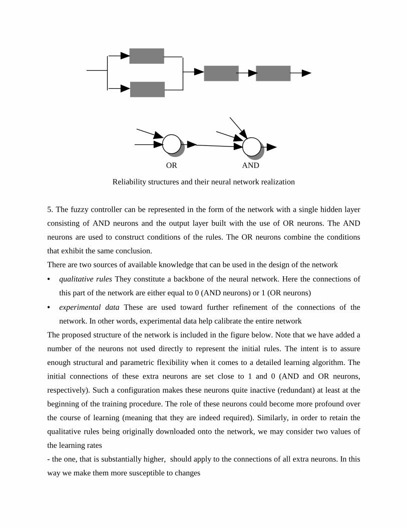
ANDOR
Reliability structures and their neural network realization
5. The fuzzy controller can be represented in the form of the network with a single hidden layer
consisting of AND neurons and the output layer built with the use of OR neurons. The AND
neurons are used to construct conditions of the rules. The OR neurons combine the conditions
that exhibit the same conclusion.
There are two sources of available knowledge that can be used in the design of the network
• qualitative rules They constitute a backbone of the neural network. Here the connections of
this part of the network are either equal to 0 (AND neurons) or 1 (OR neurons)
• experimental data These are used toward further refinement of the connections of the
network. In other words, experimental data help calibrate the entire network
The proposed structure of the network is included in the figure below. Note that we have added a
number of the neurons not used directly to represent the initial rules. The intent is to assure
enough structural and parametric flexibility when it comes to a detailed learning algorithm. The
initial connections of these extra neurons are set close to 1 and 0 (AND and OR neurons,
respectively). Such a configuration makes these neurons quite inactive (redundant) at least at the
beginning of the training procedure. The role of these neurons could become more profound over
the course of learning (meaning that they are indeed required). Similarly, in order to retain the
qualitative rules being originally downloaded onto the network, we may consider two values of
the learning rates
- the one, that is substantially higher, should apply to the connections of all extra neurons. In this
way we make them more susceptible to changes

- the second, far lower than the previously used, is applied to the neurons implementing the
original rules. This helps us retain their character by exposing them to quite reduced
modifications/updates.
E1
E2
E3
DE1
DE2
E4
AND neurons
OR neurons
U1
U3
U2
additional AND neurons to accommodate eventual conditions of the rule
A neural representation of the fuzzy controller
CHAPTER 12
Fuzzy Evolutionary Computation
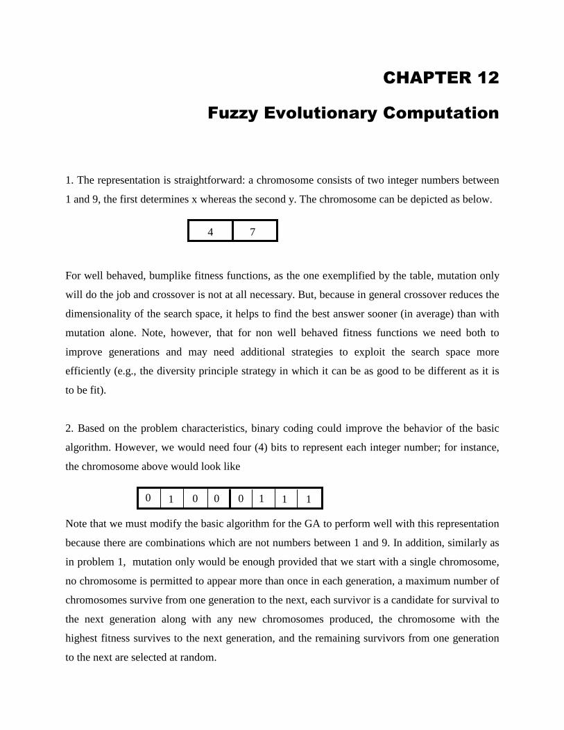
1. The representation is straightforward: a chromosome consists of two integer numbers between
1 and 9, the first determines x whereas the second y. The chromosome can be depicted as below.
For well behaved, bumplike fitness functions, as the one exemplified by the table, mutation only
will do the job and crossover is not at all necessary. But, because in general crossover reduces the
dimensionality of the search space, it helps to find the best answer sooner (in average) than with
mutation alone. Note, however, that for non well behaved fitness functions we need both to
improve generations and may need additional strategies to exploit the search space more
efficiently (e.g., the diversity principle strategy in which it can be as good to be different as it is
to be fit).
2. Based on the problem characteristics, binary coding could improve the behavior of the basic
algorithm. However, we would need four (4) bits to represent each integer number; for instance,
the chromosome above would look like
Note that we must modify the basic algorithm for the GA to perform well with this representation
because there are combinations which are not numbers between 1 and 9. In addition, similarly as
in problem 1, mutation only would be enough provided that we start with a single chromosome,
no chromosome is permitted to appear more than once in each generation, a maximum number of
chromosomes survive from one generation to the next, each survivor is a candidate for survival to
the next generation along with any new chromosomes produced, the chromosome with the
highest fitness survives to the next generation, and the remaining survivors from one generation
to the next are selected at random.
4 7
0 1 0 0 0 1 1 1
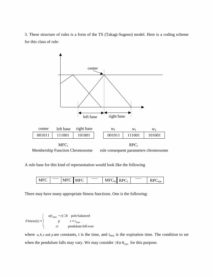
3. These structure of rules is a form of the TS (Takagi-Sugeno) model. Here is a coding scheme
for this class of rule:
Membership Function Chromosome rule consequent parameters chromosome
A rule base for this kind of representation would look like the following
There may have many appropriate fitness functions. One is the following:
=+−
=over fell pendulum
balanced pole )(
)( max
max
ct
ttp
btta
tFitness
where pcba and ,, are constants, t is the time, and tmax is the expiration time. The condition to set
when the pendulum falls may vary. We may consider max|| θ≥θ for this purpose.
center
left base right base
001011 111001 101001 001011 111001 101001
center left base right base w0 w1 w2
MFCi RPCi
MFC MFC MFC MFCm RPC1 RPCmn ...... ...... ......
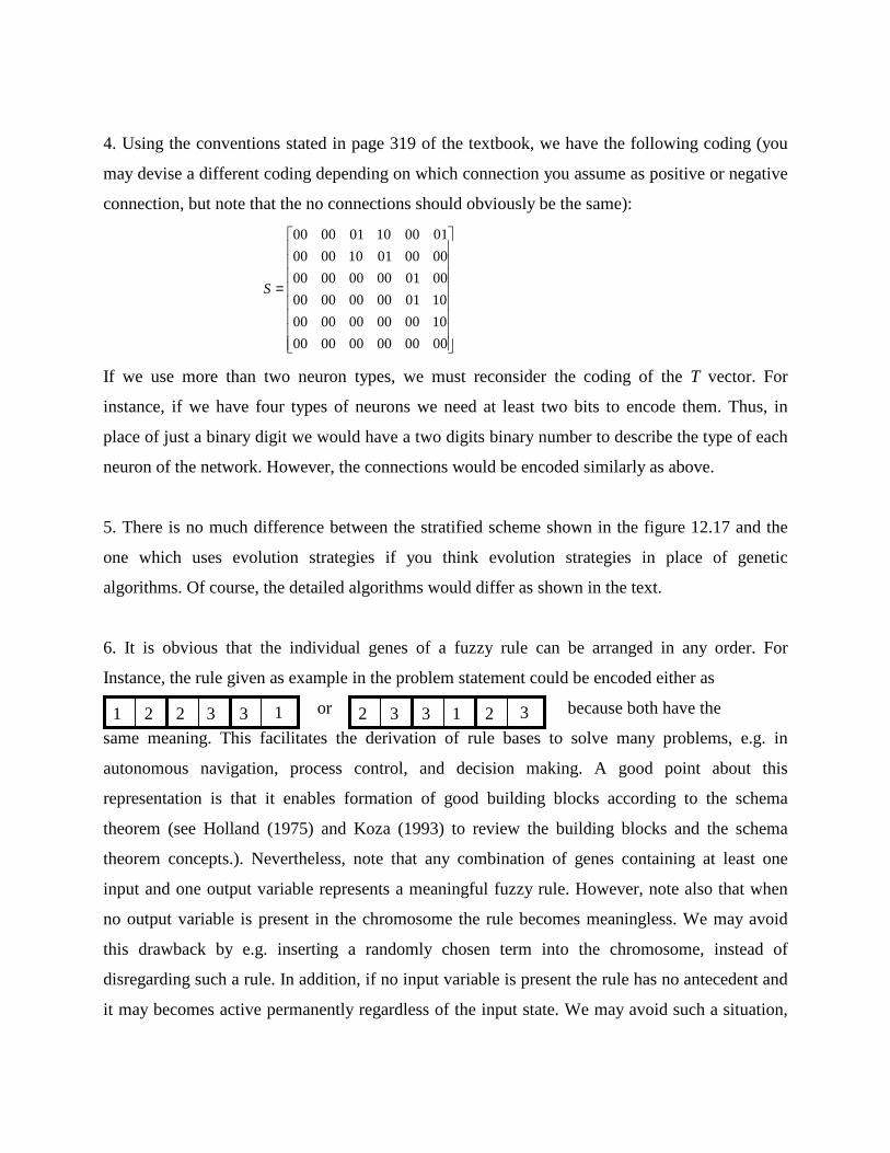
4. Using the conventions stated in page 319 of the textbook, we have the following coding (you
may devise a different coding depending on which connection you assume as positive or negative
connection, but note that the no connections should obviously be the same):
=
000000000000
100000000000
100100000000
000100000000
000001100000
010010010000
S
If we use more than two neuron types, we must reconsider the coding of the T vector. For
instance, if we have four types of neurons we need at least two bits to encode them. Thus, in
place of just a binary digit we would have a two digits binary number to describe the type of each
neuron of the network. However, the connections would be encoded similarly as above.
5. There is no much difference between the stratified scheme shown in the figure 12.17 and the
one which uses evolution strategies if you think evolution strategies in place of genetic
algorithms. Of course, the detailed algorithms would differ as shown in the text.
6. It is obvious that the individual genes of a fuzzy rule can be arranged in any order. For
Instance, the rule given as example in the problem statement could be encoded either as
or because both have the
same meaning. This facilitates the derivation of rule bases to solve many problems, e.g. in
autonomous navigation, process control, and decision making. A good point about this
representation is that it enables formation of good building blocks according to the schema
theorem (see Holland (1975) and Koza (1993) to review the building blocks and the schema
theorem concepts.). Nevertheless, note that any combination of genes containing at least one
input and one output variable represents a meaningful fuzzy rule. However, note also that when
no output variable is present in the chromosome the rule becomes meaningless. We may avoid
this drawback by e.g. inserting a randomly chosen term into the chromosome, instead of
disregarding such a rule. In addition, if no input variable is present the rule has no antecedent and
it may becomes active permanently regardless of the input state. We may avoid such a situation,
1 2 2 3 3 1 2 3 3 1 2 3

we can proceed similarly as above by adding a new randomly chosen input variable into the
chromosome.
CHAPTER 13
Fuzzy Modeling
1. In discrete case, the probabilities as well as conditional probabilities are represented in the
form of vectors and matrices. The operations used therein concern standard matrix multiplication
(in other words, Σ - product composition). When it comes to encoding we distinguish two
essential cases:
- discrete (pointwise) input. Here the probability vector assumes the form [0 0 ...0 1 0...0]
where the nonzero input refers to the current input associated with the i-th position of the
probability vector
- nonpointwise input. In this case there could be several entries of the probability vector that are
nonzero. Say, we may have [0 0 0 1/p 1/p ... 1/p 0 0 0 ]. Note that we have to adhere to the
principles of probability meaning that all entries must sum up to 1 (this is not the case in fuzzy
models).
The decoding mechanisms are these well-known in the probability calculus. Given a probability
distribution function (pdf), we convert it into a single numeric entity by considering
• mean (average)
• median
• modal, etc.
These options are well documented and discussed in depth in any comprehensive textbook on
probabilistic analysis.
2. The essence of this problem is to start from the original string of nonterminal symbols, say
aaabbb and apply production rules from the set of rules coming with the grammar G to achieve
the terminal symbol (s). First, there could be more than a single derivation for the same string.
Second, as each derivation comes with its own confidence factor determined through any t-norm,
see below, we take a maximum over all possible derivations, namely
conf(string) = maxI deri

where deri is the i-th derivation of the string; I denotes a collection of possible derivations
abccddeezzqa original string
terminal symbol
p1
pk
pc
σ
Computing a level of confidence associated with the derivation of the string; p1, p2, ... pc denote
corresponding numbers of the production rules of the grammar
3. The fuzzy sets of condition need to be distributed in such a way that they embrace the groups
of experimental data. The local models are constructed around these focal points. Note that the
type of the global model we obtain is piecewise-linear. When it comes to polynomial
approximation, we get a single (global) model. Through experimentation, we can observe that
even though the polynomial model could be highly nonlinear, we may encounter some “rippling”
effect, especially for higher-order polynomials.
4. The rule-based model of the form orients towards some selected (seed) points of the data
- if x is Ai then y =ai(x-mi) +gi
namely, the modal value of Ai equal to mi (that produces the highest activation level) and the
output is equal to gi.
Once we decide upon the form of combination of the local models, we can easily derive the
parameters of the local models using any gradient-based algorithm.
Alluding to the previous exercise, we can pick up such points around which we get a high level
of concentration of experimental data. As a matter of fact, a way of localizing such focal

elements of the model are easy in a two-dimensional case. In the multivariable case, we need to
resort ourselves to some clustering algorithms.
5. The approximation capabilities increase once we increase the number of local models by
selecting a significant number of seed points (in an extreme situation we may think of almost
any point in the data set to be used as a local model). Under such circumstances, the
generalization abilities could be almost nonexistent. If so, we have to strike a sound balance
between the number of local models and the overall generalization abilities. The optimal mixture
of approximation - generalization capabilities can be achieved through some experimentation.
6. The derivation of the gradient-based computing can be straightforward.
(a) the initial values of the parameters of the model can be established by having a closer look at
the meaning of the entries of the model’s equations. The Gaussian membership functions are
located around mi and have a spread equal to σi. These two values can be estimated from the
distribution of the data. As the linear local models are described by a free form of the linear
function (the linear models in the previous problem are more confined as passing through a given
point), there is no detailed guidelines as to the initial values of these parameters and these could
be determined through some optimization.
(b) There two distinct families of parameters. The first class concerns receptive (Gaussian) fields.
The other deal with the linear functions. As they cope with different aspects of the overall model,
they exhibit a different level of plasticity
• lower level of plasticity comes with the receptive fields. They tend to establish a more general
look at the data. Subsequently, they tend to be more “stable” and less plastic and adjustable
(low values of the learning rate)
• higher level of plasticity is encountered at the linear part of the fuzzy model. These
parameters can be adjusted more vigorously (higher values of the learning rate)
The identification of these two levels of plasticity of learning associates with the two different
values of the learning rates applied within the learning process
(c) The regularization component helps make the linguistic terms distinct; this retains their
semantics. It appears in an additive form in the overall performance index which could be viewed
as a weighted sum of these two contributing factors. To stress semantics of the linguistic terms,

we require that they do not overlap too much. In a simplest way, the level of overlap can be
quantified via the use of possibility measure, say Poss(Ai, Ai+1) where these two fuzzy sets are just
linguistic terms to be optimized. The regularization factor can embrace the possibility values
computed for all the fuzzy sets.
CHAPTER 14
Methodology
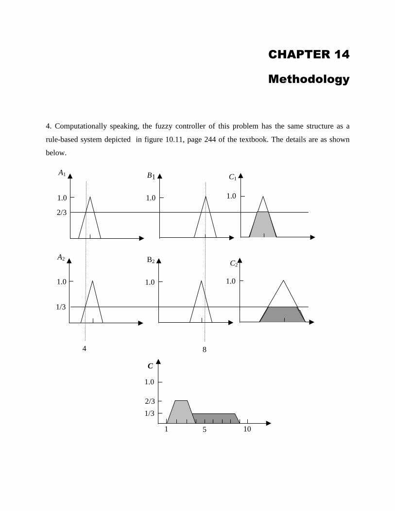
4. Computationally speaking, the fuzzy controller of this problem has the same structure as a
rule-based system depicted in figure 10.11, page 244 of the textbook. The details are as shown
below.
2/3
1.0
1.0
1.0
1.0
1.0
1.0
1/3
4 8
C1
C2 B2
B1
A2
A1
1.0
5 10 1
C
1/3
2/3

From the figure above we see that, assuming the the universe U discrete to simplify calculations,
if we use the mean-of-maxima the control is 43/)543( =++=u and if we use the center-of-
gravity we get
7.4
3
1
3
1
3
1
3
2
3
2
3
2
3
13
18
3
17
3
16
3
25
3
24
3
23
3
12
=++++++
++++++=u
Note: the numerical data was taken from Fuzzy logic controllers by H. Berenji in An Introduction
to Fuzzy Logic Applications in Intelligent Systems, R. Yager & L. Zadeh (eds), Kluwer, 1992.
6. See the figure depicted below.
7. The optimal solution can be obtained via e.g. the simplex method. See Luenberger (1973) for
the details of the simplex algorithm. It can also be trivially solved by any linear optimization
routine. The optimal solution is x1 = 1/5, x2 = 0, x3 = 8/5, the value of the objective function being
27/5. You may use MATLAB Optimization Toolbox.
8. We could proceed as follows, using the original Bellman and Zadeh approach. Thus, we may
define SIxxF −= /)( but note that while I = 0, S is unbounded. But since we know that x should
be around 1, with around being defined by the fuzzy set A(0.5,1,2) we may (subjectivelly) assume
the value of f(x) at x = 2 to define S = 4. Thus F(x) = x/4. The figure below illustrates the solution.
1.0
1.0
0.5
0.5
x1
x2
x1+ x2= 1
optimal solution
contours of the objective function

9. We must proceed as discussed in section 14.3.3.2, that is, assuming that
)4,3,2(3 =f )5.5,4,5.2(4 =f )19,18,16(18 =f )3,2,1(2 =f )2,1,5.0(1 =f )9,7,6(7 =f )5.3,3,5.2(1 =ft
and )5.1,1,5.0(2 =ft , we obtain the following auxiliary problems (see page 393 of the textbook):
maximize 5x1 + 6x2
subject to 3x1+ 4x2 ≤ 18 + 3(1 - α)
2x1+ x2 ≤ 7 + (1 - α)
x1 , x2 ≥ 0, ].1,0(∈α
maximize 5x1 + 6x2
subject to 4x1+ 5.5x2 ≤ 16 + 2.5(1 - α)
3x1+ 2 x2 ≤ 6 + 0.5 (1 - α)
x1 , x2 ≥ 0, ].1,0(∈α
Solving the two standard linear optimization problems we get:
Problem 1: x1 = 2 + 0.2(1 - α); x2 = 3 + 0.6(1 - α); objective function = 28 + 4.6(1 - α)
Problem 2: x1 = 0.11 - 0.26(1 - α); x2 = 2.82 + 0.64(1 - α); objective function = 17.53 + 2.56(1 -
α).
1.0
1.0 2.0 x
F A
x∗

The graphical solutions are easily obtained after we guess appropriate values of α. See figure
14.16. Note that we can also easily plot the optimal solutions as a function of α.
10. Clearly the answer is no! Just assume any nonlinear membership functions to model the
optimization problem data, e.g., Gaussian fuzzy coefficients, S shaped functions for tolerances in
the inequality constraints and objective functions, etc.