Embed Size (px)
Citation preview

An introduction toIsogeometric Analysis
A. Buffa1, G. Sangalli1,2, R. Vazquez1
1 Istituto di Matematica Applicata e Tecnologie Informatiche -Pavia
Consiglio Nazionale delle Ricerche
2 Dipartimento di Matematica, Universita di Pavia
Supported by the ERC Starting Grant:GeoPDEs n. 205004
R. Vazquez (IMATI-CNR Italy) Introduction to Isogeometric Analysis Santiago de Compostela, 2010 1 / 17

1 Approximation of vector fields and differential formsConstruction of the discrete spacesThe commuting De Rham diagramMaxwell eigenproblem: B-splines discretizationMaxwell eigenproblem: NURBS discretization
R. Vazquez (IMATI-CNR Italy) Introduction to Isogeometric Analysis Santiago de Compostela, 2010 2 / 17

Part I
Approximation of vector fields and differential forms
R. Vazquez (IMATI-CNR Italy) Introduction to Isogeometric Analysis Santiago de Compostela, 2010 3 / 17

Setting of the problem
Let Ω be a Lipschitz domain described by a NURBS mapping
F : Ω −→ Ω, Ω being the unit cube.
We define the functional spaces
H(d,Ω) = u ∈ L2(Ω) : du ∈ L2(Ω) , ‖u‖d,Ω = ‖u‖0 + ‖du‖0
H1(Ω)/R grad−−−−→ H(curl ,Ω)curl−−−−→ H(div,Ω)
div−−−−→ L2(Ω).
For FEM, we have the following compatible discretization
Nodal FEgrad−−−−→ Edge FE
curl−−−−→ Face FEdiv−−−−→ Disc. FE.
Approximation of vector fields: we seek for a NURBS or Splinesdiscretization compatible with this structure.
Applications: electromagnetic problems, Darcy’s flow, Stokes’ flow...
R. Vazquez (IMATI-CNR Italy) Introduction to Isogeometric Analysis Santiago de Compostela, 2010 4 / 17

Setting of the problem
Let Ω be a Lipschitz domain described by a NURBS mapping
F : Ω −→ Ω, Ω being the unit cube.
We define the functional spaces
H(d,Ω) = u ∈ L2(Ω) : du ∈ L2(Ω) , ‖u‖d,Ω = ‖u‖0 + ‖du‖0
H1(Ω)/R grad−−−−→ H(curl ,Ω)curl−−−−→ H(div,Ω)
div−−−−→ L2(Ω).
For FEM, we have the following compatible discretization
Nodal FEgrad−−−−→ Edge FE
curl−−−−→ Face FEdiv−−−−→ Disc. FE.
Approximation of vector fields: we seek for a NURBS or Splinesdiscretization compatible with this structure.
Applications: electromagnetic problems, Darcy’s flow, Stokes’ flow...R. Vazquez (IMATI-CNR Italy) Introduction to Isogeometric Analysis Santiago de Compostela, 2010 4 / 17

Vector fields - approximation in ΩBuffa, Sangalli, V., 2010
To recall some notation: univariate B-splines and NURBS
Spα/N
pα : univariate Splines/NURBS of degree p and regularity α at knots.
d
dxv : v ∈ Sp
α
≡ Sp−1
α−1
To recall some notation: multivariate B-splines and NURBS
Sp1,p2,p3α1,α2,α3
= Sp1α1⊗ Sp2
α2⊗ Sp3
α3, Np1,p2,p3
α1,α2,α3= Np1
α1⊗ Np2
α2⊗ Np3
α3.
Let us not keep track of the regularity α in what follows...
Differential operators: we look for discrete spaces in Ω such that
R −−−−→ S0grad−−−−→ S1
dcurl−−−−→ S2cdiv−−−−→ S3 −−−−→ 0
R. Vazquez (IMATI-CNR Italy) Introduction to Isogeometric Analysis Santiago de Compostela, 2010 5 / 17

Vector fields - approximation in ΩBuffa, Sangalli, V., 2010
To recall some notation: multivariate B-splines and NURBS
Sp1,p2,p3α1,α2,α3
= Sp1α1⊗ Sp2
α2⊗ Sp3
α3, Np1,p2,p3
α1,α2,α3= Np1
α1⊗ Np2
α2⊗ Np3
α3.
Let us not keep track of the regularity α in what follows...
Differential operators: we look for discrete spaces in Ω such that
R −−−−→ S0grad−−−−→ S1
dcurl−−−−→ S2cdiv−−−−→ S3 −−−−→ 0
S0 = Sp1,p2,p3
grad : S0 → Sp1−1,p2,p3 × Sp1,p2−1,p3 × Sp1,p2,p3−1 ≡ S1
R. Vazquez (IMATI-CNR Italy) Introduction to Isogeometric Analysis Santiago de Compostela, 2010 5 / 17

Vector fields - approximation in ΩBuffa, Sangalli, V., 2010
To recall some notation: multivariate B-splines and NURBS
Sp1,p2,p3α1,α2,α3
= Sp1α1⊗ Sp2
α2⊗ Sp3
α3, Np1,p2,p3
α1,α2,α3= Np1
α1⊗ Np2
α2⊗ Np3
α3.
Let us not keep track of the regularity α in what follows...
Differential operators: we look for discrete spaces in Ω such that
R −−−−→ S0grad−−−−→ S1
dcurl−−−−→ S2cdiv−−−−→ S3 −−−−→ 0
S1 = Sp1−1,p2,p3 × Sp1,p2−1,p3 × Sp1,p2,p3−1
curl : S1 → Sp1,p2−1,p3−1 × Sp1−1,p2,p3−1 × Sp1−1,p2−1,p3 ≡ S2
R. Vazquez (IMATI-CNR Italy) Introduction to Isogeometric Analysis Santiago de Compostela, 2010 5 / 17

Vector fields - approximation in ΩBuffa, Sangalli, V., 2010
To recall some notation: multivariate B-splines and NURBS
Sp1,p2,p3α1,α2,α3
= Sp1α1⊗ Sp2
α2⊗ Sp3
α3, Np1,p2,p3
α1,α2,α3= Np1
α1⊗ Np2
α2⊗ Np3
α3.
Let us not keep track of the regularity α in what follows...
Differential operators: we look for discrete spaces in Ω such that
R −−−−→ S0grad−−−−→ S1
dcurl−−−−→ S2cdiv−−−−→ S3 −−−−→ 0
S2 = Sp1,p2−1,p3−1 × Sp1−1,p2,p3−1 × Sp1−1,p2−1,p3
div : S2 → Sp1−1,p2−1,p3−1 ≡ S3
R. Vazquez (IMATI-CNR Italy) Introduction to Isogeometric Analysis Santiago de Compostela, 2010 5 / 17

Vector fields - approximation in ΩBuffa, Sangalli, V., 2010
To recall some notation: multivariate B-splines and NURBS
Sp1,p2,p3α1,α2,α3
= Sp1α1⊗ Sp2
α2⊗ Sp3
α3, Np1,p2,p3
α1,α2,α3= Np1
α1⊗ Np2
α2⊗ Np3
α3.
Let us not keep track of the regularity α in what follows...
Differential operators: we look for discrete spaces in Ω such that
R −−−−→ S0grad−−−−→ S1
dcurl−−−−→ S2cdiv−−−−→ S3 −−−−→ 0
The sequence is exact.
Generalization of nodal, edge and face elements with higher regularity.
But what about NURBS?
R. Vazquez (IMATI-CNR Italy) Introduction to Isogeometric Analysis Santiago de Compostela, 2010 5 / 17

Vector fields - approximation in ΩBuffa, Sangalli, V., 2010
To recall some notation: multivariate B-splines and NURBS
Sp1,p2,p3α1,α2,α3
= Sp1α1⊗ Sp2
α2⊗ Sp3
α3, Np1,p2,p3
α1,α2,α3= Np1
α1⊗ Np2
α2⊗ Np3
α3.
Let us not keep track of the regularity α in what follows...
Differential operators: we look for discrete spaces in Ω such that
N0grad−−−−→ N1
dcurl−−−−→ N2cdiv−−−−→ N3
The derivative of a NURBS is not a NURBS.
The diagram for NURBS does not hold true.
D. Arnold (et al.) 06-10 teach us that Ni are then not suitable for vector fields approximations
R. Vazquez (IMATI-CNR Italy) Introduction to Isogeometric Analysis Santiago de Compostela, 2010 6 / 17

Vector fields - SPLINES approximation in Ω
Spaces on Ω are defined just by push forward:
Si = ιi (Si ), Ni = ιi (Ni ).
R. Vazquez (IMATI-CNR Italy) Introduction to Isogeometric Analysis Santiago de Compostela, 2010 7 / 17

Vector fields - SPLINES approximation in Ω
Spaces on Ω are defined just by push forward:
Si = ιi (Si ), Ni = ιi (Ni ).
ι0(φ) F = φ, standard mapping
F
R. Vazquez (IMATI-CNR Italy) Introduction to Isogeometric Analysis Santiago de Compostela, 2010 7 / 17

Vector fields - SPLINES approximation in Ω
Spaces on Ω are defined just by push forward:
Si = ιi (Si ), Ni = ιi (Ni ).
ι1(u) F = DF−T u, curl conforming mapping
F
R. Vazquez (IMATI-CNR Italy) Introduction to Isogeometric Analysis Santiago de Compostela, 2010 7 / 17

Vector fields - SPLINES approximation in Ω
Spaces on Ω are defined just by push forward:
Si = ιi (Si ), Ni = ιi (Ni ).
ι2(u) F = (detDF)−1DF u, Piola mapping
F
R. Vazquez (IMATI-CNR Italy) Introduction to Isogeometric Analysis Santiago de Compostela, 2010 7 / 17

Vector fields - SPLINES approximation in Ω
Spaces on Ω are defined just by push forward:
Si = ιi (Si ), Ni = ιi (Ni ).
ι3(φ) F = (detDF)−1φ, 3-forms mapping
F
R. Vazquez (IMATI-CNR Italy) Introduction to Isogeometric Analysis Santiago de Compostela, 2010 7 / 17
Vector fields - SPLINES approximation in Ω
Spaces on Ω are defined just by push forward:
Si = ιi (Si ), Ni = ιi (Ni ).
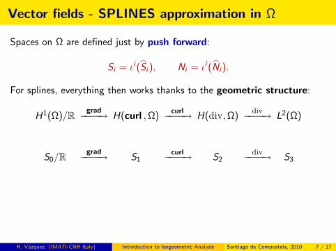
For splines, everything then works thanks to the geometric structure:
H1(Ω)/R grad−−−−→ H(curl ,Ω)curl−−−−→ H(div,Ω)
div−−−−→ L2(Ω)
Π0?y Π1?
y Π2?y Π3?
y
S0/Rgrad−−−−→ S1
curl−−−−→ S2div−−−−→ S3
How can we define the commuting interpolants Πi?
Construct (commuting) one-dimensional projectors.
Construct the projectors in Ω with tensor product structure.
Pull back from Ω to Ω.
R. Vazquez (IMATI-CNR Italy) Introduction to Isogeometric Analysis Santiago de Compostela, 2010 7 / 17

Vector fields - SPLINES approximation in Ω
Spaces on Ω are defined just by push forward:
Si = ιi (Si ), Ni = ιi (Ni ).
For splines, everything then works thanks to the geometric structure:
H1(Ω)/R grad−−−−→ H(curl ,Ω)curl−−−−→ H(div,Ω)
div−−−−→ L2(Ω)
Π0?y Π1?
y Π2?y Π3?
yS0/R
grad−−−−→ S1curl−−−−→ S2
div−−−−→ S3
How can we define the commuting interpolants Πi?
Construct (commuting) one-dimensional projectors.
Construct the projectors in Ω with tensor product structure.
Pull back from Ω to Ω.
R. Vazquez (IMATI-CNR Italy) Introduction to Isogeometric Analysis Santiago de Compostela, 2010 7 / 17

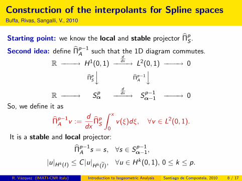
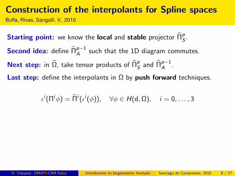
Construction of the interpolants for Spline spacesBuffa, Rivas, Sangalli, V., 2010
Starting point: we know the local and stable projector ΠpS .
ΠpSs = s, ∀s ∈ Sp
α,
|u|Hk (I ) ≤ C |u|Hk (eI )
, ∀u ∈ Hk(0, 1), 0 ≤ k ≤ p + 1,
where I = (ξj , ξj+1), and I is a local extension.L.L. Schumaker. Spline functions: basic theory, 2007.
Y. Bazilevs, L. Beirao da Veiga, J. Cottrell, T.J.R. Hughes, G. Sangalli, 2006.
Second idea: define Πp−1A such that the 1D diagram commutes.
R. Vazquez (IMATI-CNR Italy) Introduction to Isogeometric Analysis Santiago de Compostela, 2010 8 / 17

Construction of the interpolants for Spline spacesBuffa, Rivas, Sangalli, V., 2010
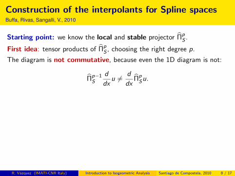
Starting point: we know the local and stable projector ΠpS .
First idea: tensor products of ΠpS , choosing the right degree p.
Second idea: define Πp−1A such that the 1D diagram commutes.
R. Vazquez (IMATI-CNR Italy) Introduction to Isogeometric Analysis Santiago de Compostela, 2010 8 / 17
Construction of the interpolants for Spline spacesBuffa, Rivas, Sangalli, V., 2010
Starting point: we know the local and stable projector ΠpS .
First idea: tensor products of ΠpS , choosing the right degree p.
The diagram is not commutative, because even the 1D diagram is not:
Πp−1S
d
dxu 6= d
dxΠp
Su.
Second idea: define Πp−1A such that the 1D diagram commutes.
R. Vazquez (IMATI-CNR Italy) Introduction to Isogeometric Analysis Santiago de Compostela, 2010 8 / 17

Construction of the interpolants for Spline spacesBuffa, Rivas, Sangalli, V., 2010
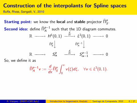
Starting point: we know the local and stable projector ΠpS .
Second idea: define Πp−1A such that the 1D diagram commutes.
R −−−−→ H1(0, 1)ddx−−−−→ L2(0, 1) −−−−→ 0
bΠpS
y bΠp−1A
yR −−−−→ Sp
α
ddx−−−−→ Sp−1
α−1 −−−−→ 0
So, we define it as
Πp−1A v :=
d
dxΠp
S
∫ x
0v(ξ)dξ, ∀v ∈ L2(0, 1).
It is a stable and local projector:
Πp−1A s = s, ∀s ∈ Sp−1
α−1,
|u|Hk (I ) ≤ C |u|Hk (eI )
, ∀u ∈ Hk(0, 1), 0 ≤ k ≤ p.
R. Vazquez (IMATI-CNR Italy) Introduction to Isogeometric Analysis Santiago de Compostela, 2010 8 / 17
Construction of the interpolants for Spline spacesBuffa, Rivas, Sangalli, V., 2010
Starting point: we know the local and stable projector ΠpS .
Second idea: define Πp−1A such that the 1D diagram commutes.
R −−−−→ H1(0, 1)ddx−−−−→ L2(0, 1) −−−−→ 0
bΠpS
y bΠp−1A
yR −−−−→ Sp
α
ddx−−−−→ Sp−1
α−1 −−−−→ 0
So, we define it as
Πp−1A v :=
d
dxΠp
S
∫ x
0v(ξ)dξ, ∀v ∈ L2(0, 1).
It is a stable and local projector:
Πp−1A s = s, ∀s ∈ Sp−1
α−1,
|u|Hk (I ) ≤ C |u|Hk (eI )
, ∀u ∈ Hk(0, 1), 0 ≤ k ≤ p.
R. Vazquez (IMATI-CNR Italy) Introduction to Isogeometric Analysis Santiago de Compostela, 2010 8 / 17

Construction of the interpolants for Spline spacesBuffa, Rivas, Sangalli, V., 2010
Starting point: we know the local and stable projector ΠpS .
Second idea: define Πp−1A such that the 1D diagram commutes.
Next step: in Ω, take tensor products of ΠpS and Πp−1
A .
For instance, for
S1 = Sp1−1,p2,p3 × Sp1,p2−1,p3 × Sp1,p2,p3−1
we define
Π1 := (Πp1−1A ⊗ Πp2
S ⊗ Πp3
S )× (Πp1
S ⊗ Πp2−1A ⊗ Πp3
S )× (Πp1
S ⊗ Πp2
S ⊗ Πp3−1A ).
R. Vazquez (IMATI-CNR Italy) Introduction to Isogeometric Analysis Santiago de Compostela, 2010 8 / 17

Construction of the interpolants for Spline spacesBuffa, Rivas, Sangalli, V., 2010
Starting point: we know the local and stable projector ΠpS .
Second idea: define Πp−1A such that the 1D diagram commutes.
Next step: in Ω, take tensor products of ΠpS and Πp−1
A .
With this choice, the diagram in Ω is commutative.
H1(Ω)/R grad−−−−→ H(curl , Ω)dcurl−−−−→ H(div, Ω)
cdiv−−−−→ L2(Ω)
bΠ0
y bΠ1
y bΠ2
y bΠ3
yS0/R
grad−−−−→ S1dcurl−−−−→ S2
cdiv−−−−→ S3
R. Vazquez (IMATI-CNR Italy) Introduction to Isogeometric Analysis Santiago de Compostela, 2010 8 / 17
Construction of the interpolants for Spline spacesBuffa, Rivas, Sangalli, V., 2010
Starting point: we know the local and stable projector ΠpS .
Second idea: define Πp−1A such that the 1D diagram commutes.
Next step: in Ω, take tensor products of ΠpS and Πp−1
A .
Last step: define the interpolants in Ω by push forward techniques.
ιi (Πiφ) = Πi (ιi (φ)), ∀φ ∈ H(d,Ω), i = 0, . . . , 3
R. Vazquez (IMATI-CNR Italy) Introduction to Isogeometric Analysis Santiago de Compostela, 2010 8 / 17

Construction of the interpolants for Spline spacesBuffa, Rivas, Sangalli, V., 2010
Starting point: we know the local and stable projector ΠpS .
Second idea: define Πp−1A such that the 1D diagram commutes.
Next step: in Ω, take tensor products of ΠpS and Πp−1
A .
Last step: define the interpolants in Ω by push forward techniques.
With the definition of these interpolants, the diagram is commutative.
H1(Ω)/R grad−−−−→ H(curl ,Ω)curl−−−−→ H(div,Ω)
div−−−−→ L2(Ω)
Π0
y Π1
y Π2
y Π3
yS0/R
grad−−−−→ S1curl−−−−→ S2
div−−−−→ S3
The projectors Πi are local and L2(Ω)-stable.
The same idea can be used in spaces with boundary conditions.R. Vazquez (IMATI-CNR Italy) Introduction to Isogeometric Analysis Santiago de Compostela, 2010 8 / 17

Approximation estimatesBuffa, Rivas, Sangalli, V., 2010.
Assume F : Ω→ Ω belongs to N0 and F−1 is piecewise regular.
Let K be an element of the mesh on the physical domain: 0 ≤ ` ≤ p
‖u − Πiu‖H(d i ,K) ≤ Ch`‖u‖H`(d i ,eK)
, i = 0, . . . , 3,
As a consequence
‖u− Π1u‖H(curl ,Ω) ≤ Ch`‖u‖H`(curl ,Ω).
Reducing the continuity we can obtain estimates in terms of p.
If α = maxαi ≤ p−12 then
‖u − Πiu‖H(d i ,K) ≤ C (h/p)`‖u‖H`(d i ,eK)
, i = 0, . . . , 3.
Beirao da Veiga, Buffa, Rivas, Sangalli (2009).
R. Vazquez (IMATI-CNR Italy) Introduction to Isogeometric Analysis Santiago de Compostela, 2010 9 / 17
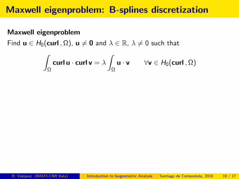
Maxwell eigenproblem: B-splines discretization
Maxwell eigenproblem
Find u ∈ H0(curl ,Ω), u 6= 0 and λ ∈ R, λ 6= 0 such that∫Ω
curl u · curl v = λ
∫Ω
u · v ∀v ∈ H0(curl ,Ω)
TheoremIf there is a commuting diagram with local and L2(Ω)-stable projectors,the Galerkin approximation is spurious-free and optimal.
D. Arnold, R. Falk, R. Winther, Bulletin A.M.S. (2010)
The B-spline discretization fulfills the theorem: it is spectrally correct.
Exact CAD description of the geometry.
Higher regularity than standard edge elements.
Singular functions are approximated correctly.
R. Vazquez (IMATI-CNR Italy) Introduction to Isogeometric Analysis Santiago de Compostela, 2010 10 / 17

Maxwell eigenproblem in the patch Ω
We solve the eigenvalue problem: Find u 6= 0 and ω 6= 0 such that
curl curl u = ω2u in Ω,
u× n = 0 on ∂Ω.
We solve with a Galerkin projection on S1,0, and different degrees p.
In terms of d.o.f., we obtain better convergence rate than edge elements.
100
10−12
10−10
10−8
10−6
10−4
10−2
100
102
p = 2
p = 3
p = 4
y = Ch4
y = Ch6
y = Ch8
Mesh size
Rel
ativ
eer
ror
101
102
103
104
10−9
10−8
10−7
10−6
10−5
10−4
10−3
10−2
10−1
IGA, p = 2
IGA, p = 3
IGA, p = 4
FEM, p = 2
FEM, p = 3
FEM, p = 4
Degrees of freedom
Rel
ativ
eer
ror
R. Vazquez (IMATI-CNR Italy) Introduction to Isogeometric Analysis Santiago de Compostela, 2010 11 / 17

Maxwell eigenproblem in the patch Ω
We solve the eigenvalue problem: Find u 6= 0 and ω 6= 0 such that
curl curl u = ω2u in Ω,
u× n = 0 on ∂Ω.
Fill-in of the matrix with respect to FEM. Sparsity pattern is similar.
0 200 400 600
0
100
200
300
400
500
600
700
nz = 334080 200 400 600
0
100
200
300
400
500
600
700
nz = 77856
R. Vazquez (IMATI-CNR Italy) Introduction to Isogeometric Analysis Santiago de Compostela, 2010 11 / 17

Maxwell eigenproblem in the patch Ω
We solve the eigenvalue problem: Find u 6= 0 and ω 6= 0 such that
curl curl u = ω2u in Ω,
u× n = 0 on ∂Ω.
We solve with continuous fields: the divergence is well defined.
It is an oscillating field, and converges to zero with order hp−1.
100
10−4
10−3
10−2
10−1
100
101
p = 2
p = 3
p = 4
y = Ch
y = Ch2
y = Ch3
Mesh size
‖div
uh‖ L
2
R. Vazquez (IMATI-CNR Italy) Introduction to Isogeometric Analysis Santiago de Compostela, 2010 11 / 17

Maxwell eigenproblem: Fichera’s corner
We solve the eigenvalue problem: Find u 6= 0 and ω 6= 0 such that
curl curl u = ω2u in Ω,u× n = 0 on ∂Ω.
Interaction between edge and corner singularities.
We get a good approximation of the singular functions.
Eigenvalues computation
CODE by S. Zaglmayr M. Durufle IGA, p = 3
d.o.f. 53982 177720 8421
Eig. 1. 3.2199939 3.2198740 3.2194306Eig. 2. 5.8804425 5.88041891 5.8804604Eig. 3. 5.8804553 5.88041891 5.8804604Eig. 4. 10.6856632 10.6854921 10.6866214Eig. 5. 10.6936955 10.6937829 10.6949643Eig. 6. 10.6937289 10.6937829 10.6949643Eig. 7. 12.3168796 12.3165205 12.3179492Eig. 8. 12.3176901 12.3165205 12.3179492
R. Vazquez (IMATI-CNR Italy) Introduction to Isogeometric Analysis Santiago de Compostela, 2010 12 / 17

Maxwell source problem: non-convex domain
We solve the source problem, with mixed boundary conditions.
curl curl u + u = f.
The geometry is described exactly with only three elements.
Domain with a reentrant edge (as the L-shaped domain).
The solution is u = grad(r2/3 sin(2θ/3)), and u ∈ H2/3−ε(curl ,Ω).
The convergence rate in energy norm is h2/3, as expected.
10−1
100
10−2
10−1
100
p = 1
p = 2
p = 3
p = 4
y = Ch2/3
Mesh size
Rel
ativ
eer
ror
R. Vazquez (IMATI-CNR Italy) Introduction to Isogeometric Analysis Santiago de Compostela, 2010 13 / 17

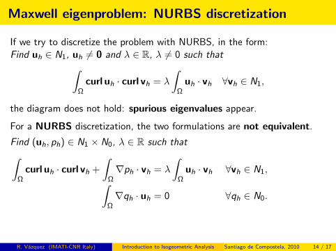
Maxwell eigenproblem: NURBS discretization
If we try to discretize the problem with NURBS, in the form:Find uh ∈ N1, uh 6= 0 and λ ∈ R, λ 6= 0 such that∫
Ωcurl uh · curl vh = λ
∫Ω
uh · vh ∀vh ∈ N1,
the diagram does not hold: spurious eigenvalues appear.
R. Vazquez (IMATI-CNR Italy) Introduction to Isogeometric Analysis Santiago de Compostela, 2010 14 / 17

Maxwell eigenproblem: NURBS discretization
If we try to discretize the problem with NURBS, in the form:Find uh ∈ N1, uh 6= 0 and λ ∈ R, λ 6= 0 such that∫
Ωcurl uh · curl vh = λ
∫Ω
uh · vh ∀vh ∈ N1,
the diagram does not hold: spurious eigenvalues appear.
−1.5 −1 −0.5 0 0.5 1 1.5
−1.5
−1
−0.5
0
0.5
1
1.5
0 50 100 150 200 2500
1
2
3
4
5
6
7
8
9
10
R. Vazquez (IMATI-CNR Italy) Introduction to Isogeometric Analysis Santiago de Compostela, 2010 14 / 17

Maxwell eigenproblem: NURBS discretization
If we try to discretize the problem with NURBS, in the form:Find uh ∈ N1, uh 6= 0 and λ ∈ R, λ 6= 0 such that∫
Ωcurl uh · curl vh = λ
∫Ω
uh · vh ∀vh ∈ N1,
the diagram does not hold: spurious eigenvalues appear.
In the continuous case, we have the equivalent mixed formulation:
Find (u, p) ∈ H0(curl ,Ω)× H10 (Ω), λ ∈ R such that∫
Ωcurl u · curl v +
∫Ω∇p · v = λ
∫Ω
u · v ∀v ∈ H0(curl ,Ω),∫Ω∇q · u = 0 ∀q ∈ H1
0 (Ω).
The two discrete formulations are equivalent for B-splines.
R. Vazquez (IMATI-CNR Italy) Introduction to Isogeometric Analysis Santiago de Compostela, 2010 14 / 17
Maxwell eigenproblem: NURBS discretization
If we try to discretize the problem with NURBS, in the form:Find uh ∈ N1, uh 6= 0 and λ ∈ R, λ 6= 0 such that∫
Ωcurl uh · curl vh = λ
∫Ω
uh · vh ∀vh ∈ N1,
the diagram does not hold: spurious eigenvalues appear.
For a NURBS discretization, the two formulations are not equivalent.
Find (uh, ph) ∈ N1 × N0, λ ∈ R such that∫Ω
curl uh · curl vh +
∫Ω∇ph · vh = λ
∫Ω
uh · vh ∀vh ∈ N1,∫Ω∇qh · uh = 0 ∀qh ∈ N0.
R. Vazquez (IMATI-CNR Italy) Introduction to Isogeometric Analysis Santiago de Compostela, 2010 14 / 17

NURBS discretization: numerical resultsBuffa, Sangalli, V. In preparation
The domain Ω is described with a NURBS mapping.
Solution of the mixed formulation with a NURBS discretization.
−1.5 −1 −0.5 0 0.5 1 1.5
−1.5
−1
−0.5
0
0.5
1
1.5
NURBS map of fine mesh10
−110
010
−10
10−8
10−6
10−4
10−2
100
3rd eigenvalue
8th eigenvalue
19th eigenvalue
y=Ch6
Mesh size
Rel
ativ
eer
ror
The results are spurious-free, with optimal convergence rate.
Also the singular functions are approximated correctly.
The spectral correctness can also be proved for (mixed) NURBS.
R. Vazquez (IMATI-CNR Italy) Introduction to Isogeometric Analysis Santiago de Compostela, 2010 15 / 17

NURBS discretization: numerical resultsBuffa, Sangalli, V. In preparation
The domain Ω is described with a NURBS mapping.
Solution of the mixed formulation with a NURBS discretization.
1 1.5 2 2.5 30
0.2
0.4
0.6
0.8
1
1.2
1.4
1.6
1.8
2
NURBS map of the coarsest mesh10
−110
−10
10−8
10−6
10−4
10−2
100
1st eigenvalue
2nd eigenvalue
3rd eigenvalue
4th eigenvalue
5th eigenvalue
y=Ch4/3
y=Ch6
Mesh size
Rel
ativ
eer
ror
The results are spurious-free, with optimal convergence rate.Also the singular functions are approximated correctly.
The spectral correctness can also be proved for (mixed) NURBS.
R. Vazquez (IMATI-CNR Italy) Introduction to Isogeometric Analysis Santiago de Compostela, 2010 15 / 17

Conclusions
Isogeometric Analysis has been extended to the approximation ofvector fields.
I Generalization of edge and face elementsI Higher continuity than standard finite elements.I Exact geometry description.
Complete theory for Maxwell, and promising numerical results.
Further comparisons with FEM will be done in the future.
COMING SOONThe GeoPDEs code: a research tool for Isogeometric Analysis of PDEs.
Open Octave (compatible with Matlab) implementation of the method.Joint work with C. de Falco and A. Reali.
http://www.imati.cnr.it/geopdes
R. Vazquez (IMATI-CNR Italy) Introduction to Isogeometric Analysis Santiago de Compostela, 2010 16 / 17

Acknowledgments
Funded by ERC Starting Grant n 205004: GeoPDEs
Team
Annalisa Buffa (IMATI-CNR)
Lourenco Beirao da Veiga (University of Milano)Alessandro Reali (University of Pavia)Giancarlo Sangalli (University of Pavia)
Andrea BressanDurkbin ChoCarlo De FalcoMukesh KumarMassimiliano MartinelliJudith RivasRafael Vazquez
Thanks for your attention!http://www.imati.cnr.it/geopdes
R. Vazquez (IMATI-CNR Italy) Introduction to Isogeometric Analysis Santiago de Compostela, 2010 17 / 17