Embed Size (px)
Citation preview
An Introduction to Linear Algebra
���������b
��������1 x1
�����
x2
HHHHj p = Ax
e = b−Ax
���������������������
��������������������
HHHHHH
HHHH
HHHH
HHHHHH
R(A)
Andreas Jakobsson
Lund University
Version 080515

i
An Introduction to Linear Algebra
These notes were written as a part of a graduate level course on transform the-ory offered at King’s College London during 2002 and 2003. The material is heavilyindebt to the excellent textbook by Gilbert Strang [1], which the reader is referredto for a more complete description of the material; for a more in-depth coverage,the reader is referred to [2–6].
Andreas [email protected]

CONTENTS
1 LINEAR ALGEBRA 11.1 Solving a set of linear equations 11.2 Vectors and matrices 21.3 Fundamental subspaces 61.4 Orthogonality 91.5 Determinants 141.6 Eigendecomposition 151.7 Singular value decomposition 191.8 Total least squares 21
A BANACH AND HILBERT SPACES 24
B THE KARHUNEN-LOEVE TRANSFORM 27
C USEFUL FORMULAE 29
BIBLIOGRAPHY 30
ii

Chapter 1
LINEAR ALGEBRA
Dimidium facti, qui coepit, habetHorace
1.1 Solving a set of linear equations
We introduce the topic of linear algebra by initially examining how to go aboutsolving a set of linear equations; say 2u + v + w = 5
4u − 6v = −2−2u + 7v + 2w = 9
(1.1.1)
By subtracting 2 times the first equation from the second equation, we obtain 2u + v + w = 5− 8v − 2w = −12
−2u + 7v + 2w = 9(1.1.2)
Term this step (i). We then add the first equation to the third equation in (1.1.2), 2u + v + w = 5− 8v − 2w = −12
8v + 3w = 14(1.1.3)
We term this step (ii). Finally, in step (iii), we add the second and third equationin (1.1.3), obtaining 2u + v + w = 5
− 8v − 2w = −12w = 2
(1.1.4)
1
2 Linear Algebra Chapter 1
This procedure is known as Gaussian1 elimination, and from (1.1.4) we can easilysolve the equations via insertion, obtaining the solution (u, v, w) = (1, 1, 2). Aneasy way to ensure that the found solution is correct is to simply insert (u, v, w)in (1.1.1). However, we will normally prefer to work with matrices instead of theabove set of equations. The matrix approach offers many benefits, as well as openingup a new way to view the equations, and we will here focus on matrices and thegeometries that can be associated with matrices.
1.2 Vectors and matrices
We proceed to write (1.1.1) on matrix form 24
−2
u +
1−6
7
v +
102
w
︸ ︷︷ ︸26642 1 14 −6 0
−2 7 2
37752664
uvw
3775
=
5−2
9
(1.2.1)
Note that we can view the columns of the matrix as vectors in a three-dimensional(real-valued) space, often written R3. This is only to say that the elements of thevectors can be viewed as the coordinates in a space, e.g., we view the third columnvector, say a3,
a3 =
102
(1.2.2)
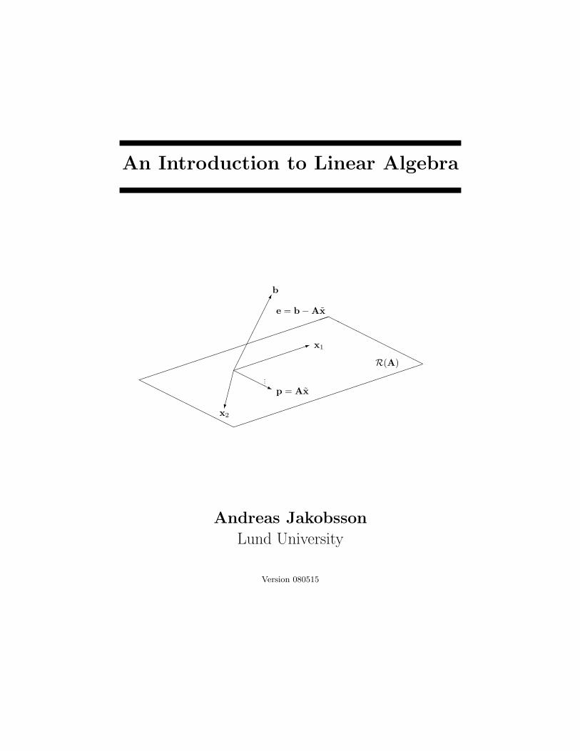
as the vector starting at origin and ending at x = 1, y = 0 and z = 2. Using asimplified geometric figure, we can depict the three column vectors as
��
��
��
��3
-������� a2
a1
a3
where the vectors are seen as lying in a three-dimensional space. The solutionto the linear set of equations in (1.1.1) is thus the scalings (u, v, w) such that if we
1Johann Carl Friedrich Gauss (1777-1855) was born in Brunswick, the Duchy of Brunswick(now Germany). In 1801, he received his doctorate in mathematics, proving the fundamentaltheorem of algebra [7]. He made remarkable contributions to all fields of mathematics, and isgenerally considered to be the greatest mathematician of all times.
Section 1.2. Vectors and matrices 3
combine the vectors asua1 + va2 + wa3 = b, (1.2.3)
we obtain the vector b, in this case b =[
5 −2 9]T , where (·)T denotes the
transpose operator. This way of viewing the linear equations also tells us when asolution exists. We say that the matrix formed from the three column vectors,
A =[
a1 a2 a3
], (1.2.4)
span the column space, i.e., the vector space containing all points reachable by anylinear combination of the column vectors of A. For example, consider
B =[
b1 b2
]=
1 00 10 0
(1.2.5)
In this case, all the points in the plane b1-b2 belongs to the column space of B;this as by combining b1 and b2 all points in the plane might be reached. However,the point b3 =
[0 0 1
]T does not lie in the column space since there is no wayto combine b1 and b2 to reach b3. Thus, it holds that
A linear set of equations is solvable if and only if the vector b liesin the column space of A.
Viewing the linear equations as vectors will be central to our treatment, and we willshortly return to this way of viewing the problem. Before doing so, we will examinehow we can view the above Gaussian elimination while working on the matrix form.
We can view the elimination in step (i) above as a multiplication by an elemen-tary matrix, E, 1 0 0
−2 1 00 0 1
︸ ︷︷ ︸
E
2 1 14 −6 0
−2 7 2
uvw
= E
5−2
9
(1.2.6)
which yields (cf. (1.1.2)) 2 1 10 −8 −2
−2 7 2
uvw
=
5−12
9
(1.2.7)
Similarly, we can view step (ii) and (iii) as multiplications with elementary matrices 1 0 00 1 00 1 1
︸ ︷︷ ︸
G
1 0 00 1 01 0 1
︸ ︷︷ ︸
F
2 1 10 −8 −2
−2 7 2
uvw
= GF
5−12
9
(1.2.8)
4 Linear Algebra Chapter 1
yielding (cf. 1.1.4)) 2 1 10 −8 −20 0 1
uvw
=
5−12
2
(1.2.9)
The resulting matrix, which we will term U, will be an upper-triangular matrix.We denote the sought solution x =
[u v w
]T , and note that we have by thematrix multiplications rewritten
Ax = b ⇒ Ux = c, (1.2.10)
where U = (GFE)A and c = (GFE)b. As U is upper-triangular, the new matrixequation is obviously trivial to solve via insertion.
We proceed by applying the inverses of the above elementary matrices (in reverseorder!), and note that
E−1F−1G−1︸ ︷︷ ︸L
GFEA︸ ︷︷ ︸U
= A. (1.2.11)
This is the so-called LU-decomposition, stating that
A square matrix that can be reduced to U (without row inter-changes2) can be written as A = LU.
As the inverse of an elementary matrix can be obtain by simply changing the signof the off-diagonal element3,
E−1 =
1 0 0−2 1 0
0 0 1
−1
=
1 0 02 1 00 0 1
(1.2.12)
we can immediately obtain the LU-decomposition after reducing A to U,
A = LU =
1 0 02 1 0
−1 −1 1
2 1 10 −8 −20 0 1
(1.2.13)
Note that L will be a lower-triangular matrix. Often, one divides out the diagonalelements of U, the so-called pivots4, denoting the diagonal matrix with the pivotson the diagonal D, i.e.,
A = LU = LDU. (1.2.14)
2Note that in some cases, row exchanges are required to reduce A to U. In such case, A cannot be written as LU. See [1] for further details on row interchanges.
3Please note that this only holds for elementary matrices!4We note that pivots are always nonzero.
Section 1.2. Vectors and matrices 5
A bit confusing, U is normally just denoted U, forcing the reader to determinewhich of the matrices are referred to from the context. For our example,
A = LDU =
1 0 02 1 0
−1 −1 1
2 0 00 −8 00 0 1
1 0.5 0.50 1 0.250 0 1
(1.2.15)
The LU-decomposition suggests an efficient approach to solve a linear set of equa-tions by first factoring the matrix as A = LU, and then solve Lc = b and Ux = c.It can be shown that the LU-decomposition of a n × n matrix requires n3/3 oper-ations, whereas the solving of the two triangular systems requires n2/2 operationseach. Thus, if we wish to solve the same set of equations (same A matrix) witha new b vector, this can be done in only n2 operations (which is significantly lessthan n3/3+n2). Often, the inherent structure of the A matrix can further simplifycalculations. For example, we will often consider symmetric matrices, i.e., matricessatisfying
A = AT , (1.2.16)
or, more generally, Hermitian5 matrices, i.e., matrices satisfying
A = AH , (1.2.17)
where (·)H denotes the Hermitian, or conjugate transpose, operator. Obviously, aHermitian matrix is also symmetric, whereas the converse is in general not true. IfA is Hermitian, and if it can be factored as A = LDU (without row exchanges todestroy the symmetry), then U = LH , i.e.,
A square Hermitian matrix that (without row interchanges) can bereduced to U, can be written as A = LDLH , where D is diagonal,and L lower-triangular.
This symmetry will simplify the computation of the LU-decomposition, reducingthe complexity to n3/6 operations. Further, in the case when the diagonal elementsof D are all positive, the LU-decomposition can be written as
A = LDLH =(LD1/2
)(LD1/2
)H
= CCH , (1.2.18)
where C is the (matrix) square root of A. However, if C is a square root of A, thenso is CB, i.e.,
A = (CB) (CB)H, (1.2.19)
5Charles Hermite (1822-1901) was born in Dieuze, France, with a defect in his right foot, makingit hard for him to move around. After studying one year at the Ecole Polytechnique, Hermite wasrefused the right to continue his studies because of this disability. However, this did not preventhis work, and in 1856 he was elected to the Academie des Sciences. After making importantcontributions to number theory and algebra, orthogonal polynomials, and elliptic functions, hewas in 1869 appointed professor of analysis both at the Ecole Polytechnique and at the Sorbonne.
6 Linear Algebra Chapter 1
for any matrix B such thatBBH = BHB = I. (1.2.20)
A matrix satisfying (1.2.20) is said to be a unitary matrix 6. Hence, there are aninfinite number of square roots of a given matrix satisfying (1.2.18). Two often usedchoices for square roots are
(i) The Hermitian square root: C = CH . The Hermitian square root is unique.
(ii) The Cholesky7 factor. If C is lower-triangular with non-negative diagonalelements, then C is called the Cholesky factor of A. This is the famousCholesky factorization of A.
We will now return to the discussion on vectors and vector spaces.
1.3 Fundamental subspaces
Recall that Ax = b is solvable if and only if the vector b lies in the column spaceof A, i.e., if it can be expressed as a combination of the column vectors of A.We will now further discuss vector spaces8, as well as different ways to representsuch a space. For instance, how can we represent this vector space using as fewvectors as possible? Can the matrix A be used to span any other vector spaces?To answer these questions, we will discuss what it means to span a space, and somematters that concern vector spaces. We begin with the central definition of lineardependence. If
c1v1 + · · ·+ ckvk = 0 only happens when c1 = c2 = · · · = ck = 0 (1.3.1)
then the vectors v1, . . . ,vk are linearly independent. Otherwise, at least one of thevectors is a linear combination of the others. The number of linearly independentcolumns of a matrix is termed the column rank of the matrix. If the matrix consistsof only linearly independent column vectors, one say that it has full column rank.For example, consider
A =
1 3 3 22 6 9 5
−1 −3 3 0
(1.3.2)
6In the case of real-valued data, (1.2.20) can be written as BBT = BT B = I. Such a matrix issaid to be an orthogonal matrix. Here, the term orthonormal matrix would be more appropriate,but this term is not commonly used.
7Andre-Louis Cholesky (1875-1918) was born in Montguyon, France. He was a French militaryofficer involved in geodesy and surveying in Crete and North Africa just before World War I. Hedeveloped the method now named after him to compute solutions to the normal equations forsome least squares data fitting problems arising in geodesy. He died in battle during the war, hiswork published posthumously.
8See appendix A for a further discussion on vector spaces.
Section 1.3. Fundamental subspaces 7
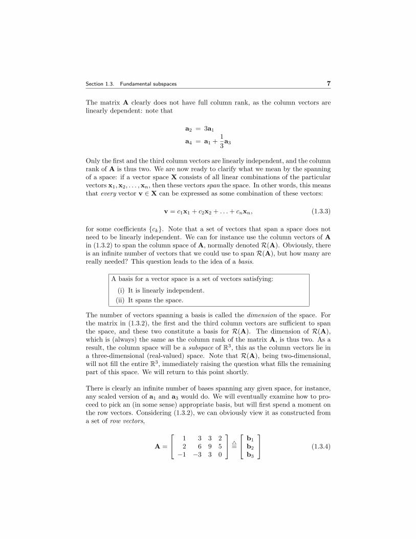
The matrix A clearly does not have full column rank, as the column vectors arelinearly dependent: note that
a2 = 3a1
a4 = a1 +13a3
Only the first and the third column vectors are linearly independent, and the columnrank of A is thus two. We are now ready to clarify what we mean by the spanningof a space: if a vector space X consists of all linear combinations of the particularvectors x1,x2, . . . ,xn, then these vectors span the space. In other words, this meansthat every vector v ∈ X can be expressed as some combination of these vectors:
v = c1x1 + c2x2 + . . . + cnxn, (1.3.3)
for some coefficients {ck}. Note that a set of vectors that span a space does notneed to be linearly independent. We can for instance use the column vectors of Ain (1.3.2) to span the column space of A, normally denoted R(A). Obviously, thereis an infinite number of vectors that we could use to span R(A), but how many arereally needed? This question leads to the idea of a basis.
A basis for a vector space is a set of vectors satisfying:
(i) It is linearly independent.(ii) It spans the space.
The number of vectors spanning a basis is called the dimension of the space. Forthe matrix in (1.3.2), the first and the third column vectors are sufficient to spanthe space, and these two constitute a basis for R(A). The dimension of R(A),which is (always) the same as the column rank of the matrix A, is thus two. As aresult, the column space will be a subspace of R3, this as the column vectors lie ina three-dimensional (real-valued) space. Note that R(A), being two-dimensional,will not fill the entire R3, immediately raising the question what fills the remainingpart of this space. We will return to this point shortly.
There is clearly an infinite number of bases spanning any given space, for instance,any scaled version of a1 and a3 would do. We will eventually examine how to pro-ceed to pick an (in some sense) appropriate basis, but will first spend a moment onthe row vectors. Considering (1.3.2), we can obviously view it as constructed froma set of row vectors,
A =
1 3 3 22 6 9 5
−1 −3 3 0
4=
b1
b2
b3
(1.3.4)
8 Linear Algebra Chapter 1
where
b1 =[
1 3 3 2]
(1.3.5)
b2 =[
2 6 9 5]
(1.3.6)
b3 =[−1 −3 3 0
](1.3.7)
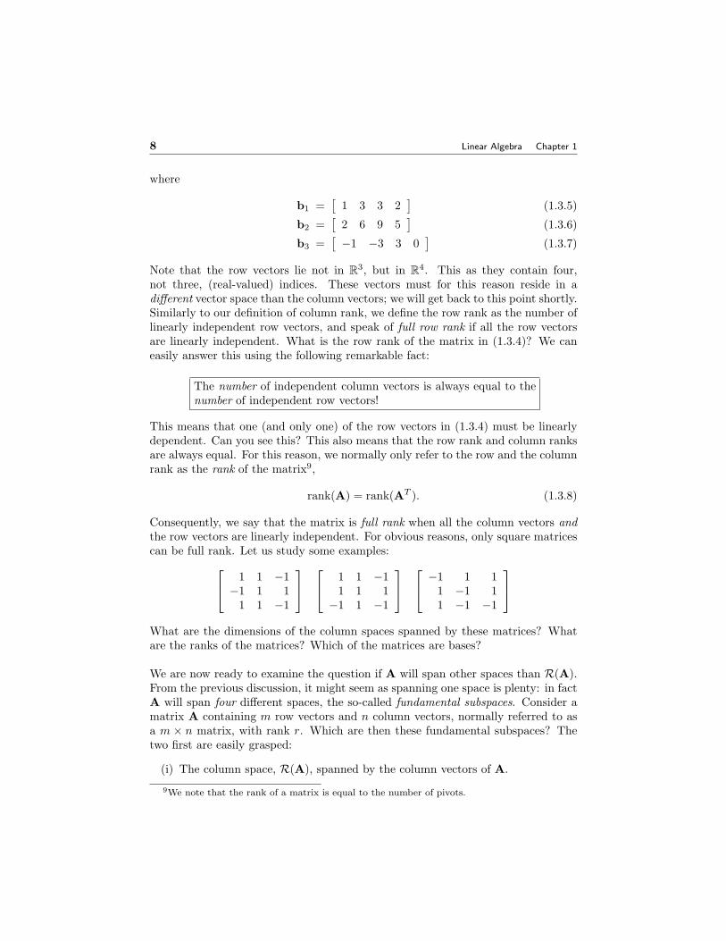
Note that the row vectors lie not in R3, but in R4. This as they contain four,not three, (real-valued) indices. These vectors must for this reason reside in adifferent vector space than the column vectors; we will get back to this point shortly.Similarly to our definition of column rank, we define the row rank as the number oflinearly independent row vectors, and speak of full row rank if all the row vectorsare linearly independent. What is the row rank of the matrix in (1.3.4)? We caneasily answer this using the following remarkable fact:
The number of independent column vectors is always equal to thenumber of independent row vectors!
This means that one (and only one) of the row vectors in (1.3.4) must be linearlydependent. Can you see this? This also means that the row rank and column ranksare always equal. For this reason, we normally only refer to the row and the columnrank as the rank of the matrix9,
rank(A) = rank(AT ). (1.3.8)
Consequently, we say that the matrix is full rank when all the column vectors andthe row vectors are linearly independent. For obvious reasons, only square matricescan be full rank. Let us study some examples: 1 1 −1
−1 1 11 1 −1
1 1 −11 1 1
−1 1 −1
−1 1 11 −1 11 −1 −1
What are the dimensions of the column spaces spanned by these matrices? Whatare the ranks of the matrices? Which of the matrices are bases?
We are now ready to examine the question if A will span other spaces than R(A).From the previous discussion, it might seem as spanning one space is plenty: in factA will span four different spaces, the so-called fundamental subspaces. Consider amatrix A containing m row vectors and n column vectors, normally referred to asa m × n matrix, with rank r. Which are then these fundamental subspaces? Thetwo first are easily grasped:
(i) The column space, R(A), spanned by the column vectors of A.
9We note that the rank of a matrix is equal to the number of pivots.
Section 1.4. Orthogonality 9
(ii) The row space, R(AT ), spanned by the row vectors of A.
Both these spaces will have dimension r, as the number of linearly independentcolumn vectors equal the number of linearly independent row vectors. The tworemaining subspaces consist of the so-called nullspaces. Consider a vector x suchthat
Ax = 0. (1.3.9)
Obviously the null vector, x = 0, will satisfy this, but other vectors may do so aswell. Any vector, other than the null vector, satisfying (1.3.9) is said to lie in thenullspace of A. Similarly, we denote the space spanned by the vectors y, such that
yT A = 0, (1.3.10)
the left nullspace of A, this to denote that the vector y multiply A from the left10.The two final fundamental subspaces are thus:
(iii) The nullspace, N (A), is spanned by the vectors x satisfying (1.3.9).
(iv) The left nullspace, N (AT ), is spanned by the vectors y satisfying (1.3.10).
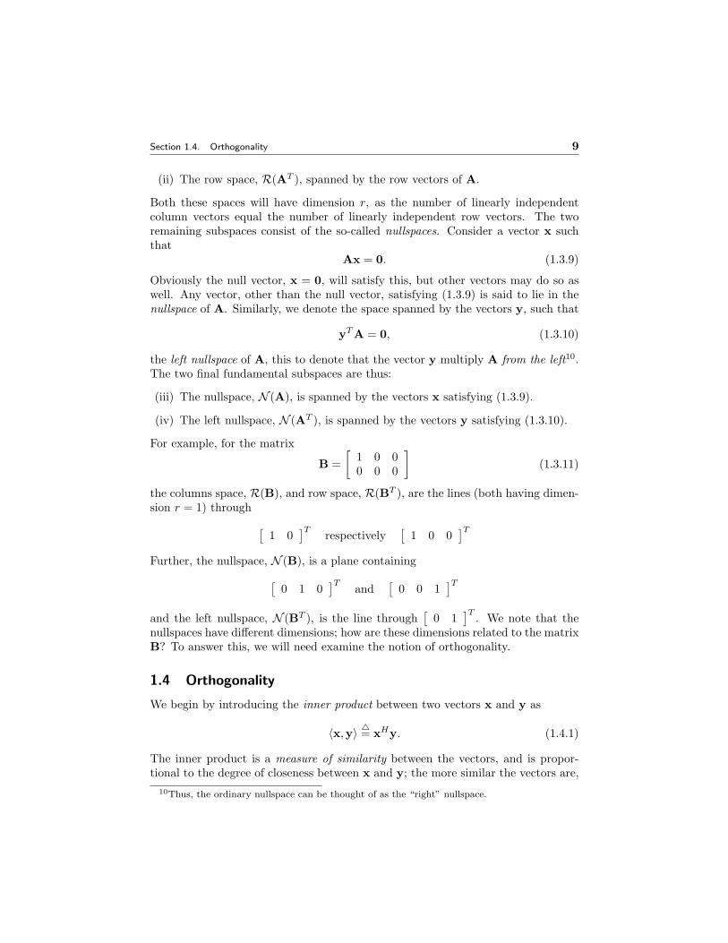
For example, for the matrix
B =[
1 0 00 0 0
](1.3.11)
the columns space, R(B), and row space, R(BT ), are the lines (both having dimen-sion r = 1) through [
1 0]T respectively
[1 0 0
]TFurther, the nullspace, N (B), is a plane containing[
0 1 0]T and
[0 0 1
]Tand the left nullspace, N (BT ), is the line through
[0 1
]T . We note that thenullspaces have different dimensions; how are these dimensions related to the matrixB? To answer this, we will need examine the notion of orthogonality.
1.4 Orthogonality
We begin by introducing the inner product between two vectors x and y as
〈x,y〉 4= xHy. (1.4.1)
The inner product is a measure of similarity between the vectors, and is propor-tional to the degree of closeness between x and y; the more similar the vectors are,
10Thus, the ordinary nullspace can be thought of as the “right” nullspace.
10 Linear Algebra Chapter 1
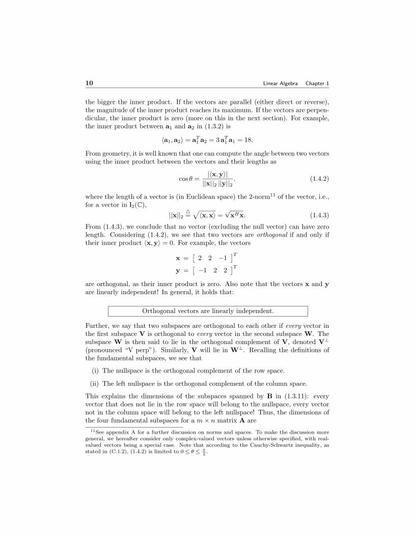
the bigger the inner product. If the vectors are parallel (either direct or reverse),the magnitude of the inner product reaches its maximum. If the vectors are perpen-dicular, the inner product is zero (more on this in the next section). For example,the inner product between a1 and a2 in (1.3.2) is
〈a1,a2〉 = aT1 a2 = 3aT
1 a1 = 18.
From geometry, it is well known that one can compute the angle between two vectorsusing the inner product between the vectors and their lengths as
cos θ =|〈x,y〉|
||x||2 ||y||2. (1.4.2)
where the length of a vector is (in Euclidean space) the 2-norm11 of the vector, i.e.,for a vector in l2(C),
||x||24=√〈x,x〉 =
√xHx. (1.4.3)
From (1.4.3), we conclude that no vector (excluding the null vector) can have zerolength. Considering (1.4.2), we see that two vectors are orthogonal if and only iftheir inner product 〈x,y〉 = 0. For example, the vectors
x =[
2 2 −1]T
y =[−1 2 2
]Tare orthogonal, as their inner product is zero. Also note that the vectors x and yare linearly independent! In general, it holds that:
Orthogonal vectors are linearly independent.
Further, we say that two subspaces are orthogonal to each other if every vector inthe first subspace V is orthogonal to every vector in the second subspace W. Thesubspace W is then said to lie in the orthogonal complement of V, denoted V⊥
(pronounced “V perp”). Similarly, V will lie in W⊥. Recalling the definitions ofthe fundamental subspaces, we see that
(i) The nullspace is the orthogonal complement of the row space.
(ii) The left nullspace is the orthogonal complement of the column space.
This explains the dimensions of the subspaces spanned by B in (1.3.11): everyvector that does not lie in the row space will belong to the nullspace, every vectornot in the column space will belong to the left nullspace! Thus, the dimensions ofthe four fundamental subspaces for a m× n matrix A are
11See appendix A for a further discussion on norms and spaces. To make the discussion moregeneral, we hereafter consider only complex-valued vectors unless otherwise specified, with real-valued vectors being a special case. Note that according to the Cauchy-Schwartz inequality, asstated in (C.1.2), (1.4.2) is limited to 0 ≤ θ ≤ π
2.
Section 1.4. Orthogonality 11
(i) dim{R(A)} = rank{A} = r
(ii) dim{R(AT )
}= r
(iii) dim{N (A)} = n− r.
(iv) dim{N (AT )
}= m− r.
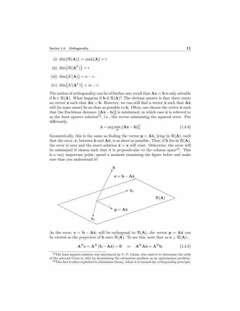
The notion of orthogonality can be of further use; recall that Ax = b is only solvableif b ∈ R(A). What happens if b /∈ R(A)? The obvious answer is that there existsno vector x such that Ax = b. However, we can still find a vector x such that Axwill (in some sense) lie as close as possible to b. Often, one choose the vector x suchthat the Euclidean distance ‖Ax− b‖22 is minimized, in which case x is referred toas the least squares solution12, i.e., the vector minimizing the squared error. Putdifferently,
x = arg minx‖Ax− b‖22 (1.4.4)
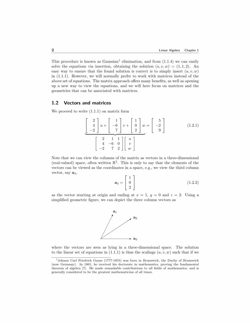
Geometrically, this is the same as finding the vector p = Ax, lying in R(A), suchthat the error, e, between b and Ax, is as short as possible. Thus, if b lies in R(A),the error is zero and the exact solution x = x will exist. Otherwise, the error willbe minimized if chosen such that it is perpendicular to the column space13. Thisis a very important point; spend a moment examining the figure below and makesure that you understand it!
���������b
��������1 x1
�����
x2
HHHHj p = Ax
e = b−Ax
���������������������
��������������������
HHHHHH
HHHH
HHHHHH
HHHH
R(A)
As the error, e = b − Ax, will be orthogonal to R(A), the vector p = Ax canbe viewed as the projection of b onto R(A). To see this, note that as e ⊥ R(A),
AHe = AH (b−Ax) = 0 ⇒ AHAx = AHb. (1.4.5)
12The least squares solution was introduced by C. F. Gauss, who used it to determine the orbitof the asteroid Ceres in 1821 by formulating the estimation problem as an optimization problem.
13This fact is often exploited in estimation theory, where it is termed the orthogonality principle.
12 Linear Algebra Chapter 1
Using the fact that
If the A has linearly independent columns, then AHA is square,Hermitian and invertible.
we obtainx =
(AHA
)−1AHb
4= A†b, (1.4.6)
where A† denotes the Moore-Penrose pseudoinverse of A. The projection of b ontoR(A) is thus
p = Ax = A(AHA
)−1AHb = AA†b
4= ΠAb, (1.4.7)
where ΠA is the projection matrix onto R(A). What would happen if you wouldproject p onto R(A)? In other words, what is Π2
Ab? How can you explain thisgeometrically? Another point worth noting is that
e = b−Ax = b−ΠAb = (I−ΠA)b4= Π⊥
Ab, (1.4.8)
where Π⊥A is the projection matrix onto the space orthogonal to R(A), i.e., Π⊥
A isthe projection matrix onto the left nullspace. Minimizing the error vector is thusthe same thing as minimizing the projection of b onto the left nullspace, i.e., wewrite b = ΠAb + Π⊥
Ab and find the vector x such that
x = arg minx‖Π⊥
Ab‖22, (1.4.9)
which is equivalent to the expression in (1.4.4). As an example, lets examine anoverdetermined (m > n) system 1 1
1 −1−1 1
︸ ︷︷ ︸
A
x =
111
︸ ︷︷ ︸
b
(1.4.10)
As b does not lie in R(A) (show this!), no solution will exist. The closest solution,in the least squares sense, can be found as
x = A†b =[
0.50.5
](1.4.11)
which corresponds to
p = Ax = ΠAb =[
1 0 0]T (1.4.12)
Verify that the error vector is orthogonal to the column space by computing theangle between b−Ax and the columns of A!
Section 1.4. Orthogonality 13
We now proceed to discuss how to find an orthogonal basis for a given space,say R(A); as commented earlier, a basis is formed by a set of linearly independentvector spanning the space. By necessity, this set must contain r = rank {A} vectors(why?), but obviously there exist an infinite number of such vector sets. We arehere interested in finding an orthogonal set of vectors using A. This can be done ina series of projection termed the Gram-Schmidt orthogonalization which will nowbe described briefly; consider the matrix
A =[
a1 . . . an
](1.4.13)
and choose the first basis vector, q1, as
q1 =a1
‖a1‖2(1.4.14)
Note that due to the normalization, q1 has unit length, we say it is a unit vector.The second basis vector should be orthogonal to q1, and for this reason we form
q′2 = a2 − 〈q1,a2〉q1 (1.4.15)
and choose the second basis vector as
q2 =q′2
‖q′2‖2(1.4.16)
The second basis vector is thus formed from a2, but with the component in thedirection of q1 subtracted out. Note that (1.4.15) can be written as
q′2 = a2 − qH1 a2q1 = a2 − q1
(qH
1 q1
)−1qH
1︸ ︷︷ ︸Πq1
a2 = Π⊥q1
a2 (1.4.17)
where we used the fact that ‖q1‖ = 1. Thus, the second vector is nothing butthe projection of a2 onto the space orthogonal to R(q1); as a result it must beorthogonal to q1. Due to the normalization in (1.4.14) and (1.4.16), the two vectorsare orthonormal, i.e., they are orthogonal unit vectors. We proceed to construct
Q =[
q1 q2
](1.4.18)
and form q3 to be orthonormal to the vectors in Q, i.e.,
q3 =Π⊥
Qa3∥∥∥Π⊥Qa3
∥∥∥2
(1.4.19)
By adding q3 to Q and repeating the projections, we can in this manner constructthe orthonormal basis. Written in matrix form, this yields
A = QR =[
q1 . . . qn
]〈q1,a1〉 〈q1,a2〉 . . . 〈q1,an〉
〈q2,a2〉 . . . 〈q2,an〉. . .
...0 〈qn,an〉
(1.4.20)
14 Linear Algebra Chapter 1
where the m× n matrix Q forms the orthonormal basis, and R is upper triangularand invertible. This is the famous Q-R factorization. Note that A does not needto be a square matrix to be written as in (1.4.20); however, if A is a square matrix,then Q is a unitary matrix. In general:
If A ∈ Cm×n, with m ≥ n, there is a matrix Q ∈ Cm×n withorthonormal columns and an upper triangular matrix R ∈ Cn×n
such that A = QR. If m = n, Q is unitary; if in addition A isnonsingular, then R may be chosen so that all its diagonal entriesare positive. In this case, the factors Q and R are unique.
The Q-R factorization concludes our discussion on orthogonality, and we proceedto dwell on the notion of determinants.
1.5 Determinants
As we have seen above, we often wish to know when a square matrix is invertible14.The simple answer is:
A matrix A is invertible, when the determinant of the matrix isnon-zero, i.e., det{A} 6= 0.
That is a good and short answer, but one that immediately raises another question.What is then the determinant? This is less clear cut to answer, being somewhatelusive. You might say that the determinant is a number that capture the soul ofa matrix, but for most this is a bit vague. Let us instead look at the definition ofthe determinant; for a 2 by 2 matrix it is simple:
det[
a11 a12
a21 a22
]=∣∣∣∣ a11 a12
a21 a22
∣∣∣∣ = a11a22 − a12a21 (1.5.1)
For a larger matrix, it is more of a mess. Then,
detA = ai1Ai1 + · · ·+ ainAin, (1.5.2)
where the cofactor Aij isAij = (−1)i+j detMij (1.5.3)
and the matrix Mij is formed by deleting row i and column j of A (see [1] for furtherexamples of the use of (1.5.2) and (1.5.3)). Often, one can use the properties of thedeterminant to significantly simplify the calculations. The main properties are
(i) The determinant depends linearly on the first row.∣∣∣∣ a + a′ b + b′
c d
∣∣∣∣ = ∣∣∣∣ a bc d
∣∣∣∣+ ∣∣∣∣ a′ b′
c d
∣∣∣∣ (1.5.4)
14We note in passing that the inverse does not exist for non-square matrices; however, suchmatrices might still have a left or a right inverse.
Section 1.6. Eigendecomposition 15
(ii) The determinant change sign when two rows are exchanged.∣∣∣∣ a bc d
∣∣∣∣ = −∣∣∣∣ c d
a b
∣∣∣∣ (1.5.5)
(iii) det I = 1.
Given these three basic properties, one can derive numerous determinant rules. Wewill here only mention a few convenient rules, leaving the proofs to the interestedreader (see, e.g., [1, 6]).
(iv) If two rows are equal, then detA = 0.
(v) If A has a zero row, then detA = 0.
(vi) Subtracting a multiple of one row from another leaves the detA unchanged.
(vii) If A is triangular, then detA is equal to the product of the main diagonal.
(viii) If A is singular, detA = 0.
(ix) detAB = (detA)(detB)
(x) detA = detAT .
(xi) |cA| = cn |A|, for c ∈ C.
(xii) det(A−1
)= (detA)−1.
(xiii) |I−AB| = |I−BA|.
where A,B ∈ Cn×n. Noteworthy is that the determinant of a singular matrix iszero. Thus, as long as the determinant of A is non-zero, the matrix A will benon-singular and invertible. We will make immediate use of this fact.
1.6 Eigendecomposition
We now move to study eigenvalues and eigenvectors. Consider a square matrix A.By definition, x is an eigenvector of A if it satisfies
Ax = λx. (1.6.1)
That is, if multiplied with A, it will only yield a scaled version of itself. Note that(1.6.1) implies that
(A− λI)x = 0, (1.6.2)
requiring x to be in N (A−λI). We require that the eigenvector x must be non-zero,and as a result, A− λI must be singular15, i.e., the scaling λ is an eigenvalue of Aif and only if
det (A− λI) = 0. (1.6.3)15Otherwise, the nullspace would not contain any vectors, leaving only x = 0 as a solution.

16 Linear Algebra Chapter 1
The above equation is termed the characteristic equation, and also points to howone should go about computing the eigenvalues of a matrix. For example, let
A =[
4 −52 −3
](1.6.4)
and thus,
det (A− λI) =∣∣∣∣ 4− λ −5
2 −3− λ
∣∣∣∣ = (4− λ)(−3− λ) + 10 = 0, (1.6.5)
or λ = −1 or 2. By inserting the eigenvalues into (1.6.1), we obtain
x1 =[
11
]and x2 =
[52
](1.6.6)
The eigendecomposition is a very powerful tool in data processing, and is frequentlyused in a variety of algorithms. One reason for this is that:
If A has n distinct eigenvalues, then A has n linearly independenteigenvectors, and is diagonalizable.
If A has n linearly independent eigenvectors, then if placed as columns of a matrixS, we can diagonalize A as
S−1AS = Λ4=
λ1
. . .λn
⇔ A = SΛS−1. (1.6.7)
That is, A is similar to a diagonal matrix. In general, we say a matrix B is similarto a matrix A is there exists a nonsingular matrix S such that
B = SAS−1. (1.6.8)
The transformation A → SAS−1 is often called a similarity transformation by thesimilarity matrix S. We note that:
If A and B are similar, then they have the same eigenvalues.
To illustrate the importance of (1.6.7), we note as an example that it immediatelyimplies that
Ak = SΛkS−1. (1.6.9)
Check this for A2 using (1.6.4). Similarly,
A−1 = SΛ−1S−1, (1.6.10)
Section 1.6. Eigendecomposition 17
with Λ−1 having{λ−1
k
}as diagonal elements. Check! We proceed with some obser-
vations; the eigenvalues of AT are the same as those of A, whereas the eigenvaluesof AH are the complex conjugate of those of A. Further,
n∏k=1
λk = detA (1.6.11)
n∑k=1
λk = trA (1.6.12)
where trA denotes the trace16 of A, i.e, the sum of the diagonal elements of A.Check this for the example in (1.6.4). Note that eigenvalues can be complex-valued,and can be zero. As mentioned, we are often encountering Hermitian matrices. Inthis case:
A Hermitian matrix has real-valued eigenvalues and eigenvectorsforming an orthonormal set.
Thus, for a Hermitian matrix, (1.6.7) can be written as
A = UΛUH =n∑
k=1
λkxkxHk (1.6.13)
where U is a unitary matrix whose columns are the eigenvectors of A. Equation(1.6.13) is often referred to as the spectral theorem. Note that xkxH
k is nothing butthe projection onto the kth eigenvector, i.e.,
Πxk= xkxH
k . (1.6.14)
Using (1.6.14), one can therefore view the spectral theorem as
A =n∑
k=1
λkΠxk(1.6.15)
The eigenvectors form a basis spanning R(A). The spectral theorem is closely re-lated to the Karhunen-Loeve transform, briefly described in Appendix B.
We proceed by briefly discussing quadratic minimization; this problem is so fre-quently reoccurring (recall for instance the least squares problem in (1.4.4)) that itdeserves a moment of our attention. As an example, consider the minimization ofthe function
f = 2x21 − 2x1x2 + 2x2
2 − 2x2x3 + 2x23 (1.6.16)
16An often used result is the fact that tr {AB} = tr {BA}.
18 Linear Algebra Chapter 1
Finding the minimum is easily done by setting the partial derivatives to zero, yield-ing x1 = x2 = x3 = 0. But which solution different from the zero solution minimizes(1.6.16)? Rewriting (1.6.16) as
f =[
x1 x2 x3
] 2 −1 0−1 2 −1
0 −1 2
x1
x2
x3
= xT Ax (1.6.17)
we conclude that it must be A that determines the minimum of f . Let
λ1 ≥ λ2 ≥ . . . ≥ λn
and define the Rayleigh’s quotient
R(x) =xHAxxHx
(1.6.18)
Then, according to the Rayleigh-Ritz theorem, it holds that
λ1 ≥xHAxxHx
≥ λn (1.6.19)
and that R(x) is minimized by the eigenvector corresponding to the minimum eigen-value, λn. Similarly, R(x) is maximized by the dominant eigenvector, correspondingto the largest eigenvalue, λ1. For our example, the eigenvalues of A are λ1 = 3.41,λ2 = 2 and λ3 = 0.58. The minimum of f , excluding the zero solution, is thus 0.58,obtained for
x1 =[
0.5 0.7071 0.5]T
Concluding this section, we introduce the notion of positive definiteness.
The Hermitian matrix A is said to be positive definite if and onlyif xHAx can be written as a sum of n independent squares, i.e.,
xHAx > 0, ∀x (except x = 0)
If we also allow for equality, A is said to positive semi-definite. Note that
Axi = λixi ⇒ xHi Axi = λixH
i xi = λ (1.6.20)
as the eigenvectors are orthonormal. We conclude that a positive definite matrixhas positive eigenvalues. The reverse is also true; if a matrix has only positiveeigenvalues, it is positive definite (the proof is left as an exercise for the reader).
The Hermitian matrix A is said to be positive definite if and onlyif A has positive (real-valued) eigenvalues.
In passing, we note that if A is positive semi-definite, it implies that there exists amatrix C (of rank n) such that A = CCH (compare with the discussion at the endof Section 1.2). For this case, we note that R(A) = R(C).
Section 1.7. Singular value decomposition 19
1.7 Singular value decomposition
As mentioned in previous section, the eigendecomposition in (1.6.7) is a very pow-erful tool, finding numerous applications in all fields of signal processing. However,the decomposition is limited by the fact that it only exists for square matrices. Wewill now proceed to study the more general case.
Every matrix A ∈ Cm×n can be factored as
A = UΣVH
where Σ ∈ Rm×n is diagonal, and U ∈ Cm×m, V ∈ Cn×n areunitary matrices.
This is the famous singular value decomposition17 (SVD), being one of the mostpowerful tools in signal processing. The diagonal elements of Σ,
Σ =
σ1
. . .σp
0. . .
0
(1.7.1)
are denoted the singular values of A. Here, p = rank(A) ≤ min(m,n), and σk ≥ 0;in general
σ1 ≥ σ2 ≥ . . . ≥ σp ≥ 0
We note thatAHA = VΣHΣVH ⇒ AHAV = VΣHΣ (1.7.2)
which implies that σ2i are the eigenvalues of AHA (similarly, it is easy to show that
σ2i are the eigenvalues of AAH). In the special case when A is a square matrix, the
17The singular value decomposition has a rich history, dating back to the independent work bythe Italian differential geometer E. Beltrami in 1873 and the French algebraist C. Jordan in 1874.Later, J. J. Sylvester in 1889, being unaware of the previous work by Beltrami and Jordan, gavea third proof for the factorization. Neither of these used the term singular values, and their workwas repeatedly rediscovered up to 1939 when C. Eckart and G. Young gave a clear and completestatement of the decomposition for a rectangular matrix. In parallel to the algebraists work, re-searchers working with the theory of integral equations rediscovered the decomposition. In 1907,E. Schmidt published a general theory for symmetric and nonsymmetric kernels, making use ofthe decomposition. In 1919, E. Picard’s generalized this theory, coining Schmidt’s “eigenvalues”as singular values (“valeurs singulieres”). It took many years of rediscovering the decomposition,under different names, until A. Horn in 1954 writing a paper on matrix theory used the term“singular values” in the context of matrices, a designation that have since become standard ter-minology (it should be noted that in the Russian literature, one also sees singular values referredto as s-numbers).

20 Linear Algebra Chapter 1
singular values coincide with the modulus of the eigenvalues18. Further, we notethat as only the first p = rank(A) singular values are non-zero, we can rewrite theSVD as
A =[
U1 U2
] [ Σ1
Σ2
] [VH
1
VH2
](1.7.3)
= U1Σ1VH1 (1.7.4)
=p∑
k=1
σkukvHk (1.7.5)
where Σ1 ∈ Rp×p, U1 ∈ Cm×p, U2 ∈ Cm×(n−p), V1 ∈ Cn×p, V2 ∈ Cn×(n−p), anduk and vk denote the kth column of U1 and V1, respectively. As the rank of amatrix is equal to the number of nonzero singular values, Σ2 = 0. Using (1.7.4),we can conclude that
R(A) ={
b ∈ Cm : b = Ax}
={
b ∈ Cm : b = U1Σ1VH1 x
}={
b ∈ Cm : b = U1y}
= span (U1)
The dominant singular vectors forms a basis spanning R(A)! Using a similar tech-nique, we find that
N (A) = span (V2)R(AH) = span (V1)N (AH) = span (U2)
which also yields that
ΠA = U1UH1 (1.7.6)
Π⊥A = I−U1UH
1 = U2UH2 (1.7.7)
For a moment returning to the least squares minimization in (1.4.4),
minx‖Ax− b‖22 = min
x‖UΣVHx− b‖22
= minx‖ΣVHx−UHb‖22
= minx‖Σy − b‖22 (1.7.8)
where we defined y = VHx and b = UHb. Minimizing (1.7.8) yields
y = Σ†b ⇒ x = VΣ†UHb (1.7.9)18Due to the numerical robustness of the SVD algorithm, it is in practice often preferable to use
the SVD instead of the eigenvalue decomposition to compute the eigenvalues.

Section 1.8. Total least squares 21
Comparing with (1.4.6), yields
A† = VΣ†UH (1.7.10)
and the conclusion that the least squares solution can immediately be obtainedusing the SVD. We also note that the singular values can be used to compute the2-norm of a matrix,
‖A‖2 = σ1. (1.7.11)
As is clear from the above brief discussion, the SVD is a very powerful tool findinguse in numerous applications. We refer the interested reader to [3] and [4] for furtherdetails on the theoretical and representational aspects of the SVD.
1.8 Total least squares
As an example of the use of the SVD, we will briefly touch on total least squares(TLS). As mentioned in our earlier discussion on the least squares minimization, itcan be viewed as finding the vector x such that
minx‖Ax− b‖22 (1.8.1)
Here, we are implicitly assuming that the errors are confined to the “observation”vector b, such that
Ax = b + ∆b (1.8.2)
It is often relevant to also assume the existence of errors in the “data” matrix, i.e.,
(A + ∆A)x = (b + ∆b) (1.8.3)
Thus, we seek the vector x, such that (b + ∆b) ∈ R(A+∆A), which minimize thenorm of the perturbations. Geometrically, this can be viewed as finding the vectorx minimizing the (squared) total distance, as compared to finding the minimum(squared) vertical distance; this is illustrated in the figure below for a line.
-
6
��
��
��
���
��
-
6
��
��
��
���
��
(a) LS: Minimize vertical (b) TLS: Minimize totaldistance to line. distance to line.

22 Linear Algebra Chapter 1
Let [A |B] denote the matrix obtained by concatenating the matrix A with thematrix B, stacking the columns of B to the right of the columns of A. Note that,
0 =[
A + ∆A |b + ∆b] [ x
−1
]=[
A |b] [ x
−1
]+[
∆A |∆b] [ x
−1
](1.8.4)
and let
C =[
A |b]
D =[
∆A |∆b]
(1.8.5)
Thus, in order for (1.8.4) to have a solution, the augmented vector [xT ,−1]T mustlie in the nullspace of C + D, and in order for the solution to be non-trivial, theperturbation D must be such that C + D is rank deficient19. The TLS solutionfinds the D with smallest norm that makes C + D rank deficient; put differently,the TLS solution is the vector minimizing
min∆A,∆b,x
‖ [∆A ∆b] ‖2F such that (A + ∆A)x = b + ∆b (1.8.6)
where
‖A‖2F = tr(AHA) =min (m,n)∑
k=1
σ2k (1.8.7)
denotes the Frobenius norm, with σk being the kth singular value of A. Let C ∈Cm×(n+1). Recalling (1.7.5), we write
C =n+1∑k=1
σkukvHk (1.8.8)
The matrix of rank n closest to C can be shown to be the matrix formed using onlythe n dominant singular values of C, i.e.,
C =n∑
k=1
σkukvHk (1.8.9)
Thus, to ensure that C + D is rank deficient, we let
D = −σn+1un+1vHn+1 (1.8.10)
19Recall that if C + D is full rank, the nullspace only contains the null vector.
Section 1.8. Total least squares 23
For this choice of D, C + D does not contain the vector20 vn+1, and the solutionto (1.8.4) must thus be a multiple α of vn+1, i.e.,[
x−1
]= αvn+1 (1.8.11)
yielding
xTLS = − vn+1(1 : n)vn+1(n + 1)
(1.8.12)
We note in passing that one can similarly write the solution to the TLS matrixequation (A + ∆A)X = (B + ∆B), where B ∈ Cm×k, as
XTLS = −V12V−122 (1.8.13)
if V−122 exists, where
V =[
V11 V12
V21 V22
](1.8.14)
with V11 ∈ Cn×n, V22 ∈ Ck×k and V12,VT21 ∈ Cn×k. The TLS estimate yields a
strongly consistent estimate of the true solution when the errors in the concatenatedmatrix [A b] are rowwise independently and identically distributed with zero meanand equal variance. If, in addition, the errors are normally distributed, the TLSsolution has maximum likelihood properties. We refer the interested reader to [4]and [5] for further details on theoretical and implementational aspects of the TLS.
20The vector vn+1 now lies in N (C + D).
Appendix A
BANACH AND HILBERTSPACES
Mister Data, there is a subspace communication for youStar Trek, the Next Generation
In this appendix, we will provide some further details on the notion of vector spaces,and in particular on the definition of Banach and Hilbert spaces, the latter beingthe vector space of primary interest in signal processing.
A vector space is by definition a set of vectors X for which any vectors in the set,say x1, x2 and x3, will satisfy that x1 + x2 ∈ X and αx1 ∈ X for some (possiblycomplex-valued) constant α, as well as the vector space axioms:
(1) x1 + x2 = x2 + x1 (commutability of addition),
(2) x1 + (x2 + x3) = (x1 + x2) + x3 (associativity of addition),
(3) ∃0 ∈ X : 0 + x1 = x1 (existence of null element),
(4) ∀x1 ∈ X ⇒ ∃− x1 ∈ X : x1 + (−x1) = 0 (existence of the inverse element),
(5) 1 · x1 = x1 (unitarism),
(6) α(βx1) = (αβ)x1 (associativity with respect to number multiplication),
(7) α(x1 + x2) = αx1 + αx2 (distributivity with respect to vector additism),
(8) (α + β)x1 = αx1 + βx1 (distributivity with respect to number additism).
Any element in a vector space is termed a vector. Often, we are primarily interestedin vector spaces that allow some form of distance measure, normally termed the
24
25
norm. Such a space is termed a Banach1 space. A Banach space is a complete2
vector space that admits a norm, ‖x‖. A norm always satisfies
‖x‖ ≥ 0 (A.1.1)
‖λx‖ = |λ| ‖x‖ (A.1.2)
‖x + y‖ ≤ ‖x‖+ ‖y‖ (A.1.3)
for any x, y in the Banach space and λ ∈ C. The so-called p-norm of a (complex-valued) discrete sequence, x(k), is defined as
‖x‖p
4=
( ∞∑k=−∞
|x(k)|p) 1
p
, (A.1.4)
for any integer p > 0. Similarly, for a (complex-valued) continuous function, f(t),the p-norm is defined as
‖f‖p
4=(∫ ∞
−∞|f(t)|p dt
) 1p
< ∞. (A.1.5)
Here, we are primarily concerned with the 2-norm, also called the Euclidean normas ‖x− y‖2 yields the Euclidean distance between any two vectors, x,y ∈ CN . Forinstance, for
x =[
1 3 2]T (A.1.6)
y =[
0 0 2]T (A.1.7)
the 2-norms are ‖x‖2 =√
12 + 32 + 22 =√
14 and ‖y‖2 = 2. Similarly, the Eu-clidean distance is ‖x− y‖2 =
√10. If not specified, we will here assume that
the used norm is the 2-norm. Note that the definitions allows for both infinite-dimensional vectors and vectors defined as continuous functions.
As is obvious from the above discussion, a Banach space is quite general, and itis often not enough to just require that a vector lies in a Banach space. For thisreason, we will further restrict our attention to work only with Banach spaces thathas an inner product (this to define angles and orthogonality). A Hilbert space is
1Stefan Banach (1892-1945) was born in Krakow, Austria-Hungary (now Poland). He receivedhis doctorate in mathematics at Lvov Technical University in 1920, and in 1924, he was promotedto full professor. He used to spend his days in the cafes of Lvov, discussing mathematics with hiscolleagues. He suffered hardship during the Nazi occupation and died of lung cancer shortly afterthe liberation. His Ph.D. thesis is often said to mark the birth of modern functional analysis.
2A complete vector space is a vector space where every Cauchy sequence converges to an elementin the space. A sequence is a Cauchy sequence if for any ε > 0, ‖x(n)− x(p)‖ < ε for large enoughn and p.
26 Banach and Hilbert spaces Appendix A
a Banach space with an inner product, 〈x,y〉. This inner product also defines thelength of a vector in the space,
‖x‖2 =√〈x,x〉. (A.1.8)
An example of a Hilbert space is l2(C), the space of “square summable sequences”,i.e., the space of (complex-valued) sequences satisfying ‖x‖2 < ∞, where the innerproduct is
〈x,y〉 = xHy =∞∑
k=−∞
x∗(k)y(k), (A.1.9)
and where (·)∗ denotes conjugate. Note that although every Hilbert space is also aBanach space, the converse need not hold. Another example is L2(C), the space ofsquare integrable functions, i.e., (complex-valued) functions satisfying ‖f‖2 < ∞,where the inner product is
〈f, g〉 =∫ ∞
−∞f∗(x)g(x) dx. (A.1.10)
In words, this means simply that the inner-product is finite, i.e., any vector in aHilbert space (even if the vector is infinite-dimensional or is a continuous function)has finite length. Obviously, this is for most practical purposes not a very strongrestriction.
Appendix B
THE KARHUNEN-LOEVETRANSFORM
E ne l’idolo suo si trasmutavaDante
In this appendix, we will briefly describe the Karhunen-Loeve transform (KLT).Among all linear transforms, the KLT is the one which best approximates a stochas-tic process in the least square sense. Furthermore, the coefficients of the KLT areuncorrelated. These properties make the KLT very interesting for many signal pro-cessing applications, such as coding and pattern recognition.
LetxN = [x1, . . . , xN ]T (B.1.1)
be a zero-mean, stationary and ergodic random process with covariance matrix (see,e.g., [8]).
Rxx = E{xNxHN} (B.1.2)
where E{·} denotes the expectation operator. The eigenvalue problem
Rxxuj = λjuj , for j = 0, . . . , N − 1, (B.1.3)
yields the j:th eigenvalue, λj , as well as the j:th eigenvector, uj . Given that Rxx isa covariance matrix1, all eigenvalues will be real and non-negative (see also Section1.6). Furthermore, N orthogonal eigenvectors can always be found, i.e.,
U = [u1, . . . ,uN ] (B.1.4)
will be a unitary matrix. The KLT of xN is found as
α = UHxN (B.1.5)
1A covariance matrix is always positive (semi) definite.
27

28 The Karhunen-Loeve transform Appendix B
where the KLT coefficients,
α = [α1, . . . , αN ]T , (B.1.6)
will be uncorrelated, i.e.,
E{αjαk} = λjδjk for j, k = 1, . . . , N. (B.1.7)
We note that this yields that
UHRxxU = Λ ⇔ Rxx = UΛUH (B.1.8)
where Λ = diag(λ1, . . . , λN ).
Appendix C
USEFUL FORMULAE
This one’s tricky. You have to use imaginary numbers, like eleventeenCalvin & Hobbes
Euler’s formula
eiωt = cos(ωt) + i sin(ωt) (C.1.1)
Cauchy-Schwartz inequality
For all x,y ∈ Cn, it hold that
〈x,y〉 ≤√〈x,x〉
√〈y,y〉 (C.1.2)
with equality if and only if x and y are dependent. Similarly, for two continuousfunctions, fx and gx, it holds that∫ ∞
−∞|fx|2 dx ·
∫ ∞
−∞|gx|2 dx ≥
∣∣∣∣∫ ∞
−∞f∗xgx dx
∣∣∣∣2 (C.1.3)
Some standard integrals
12π
∫ π
−π
eiωt dω = δt (C.1.4)∫ ∞
−∞e−ax2
dx =√
π
a(C.1.5)∫ ∞
−∞x2e−ax2
dx =12a
√π
a(C.1.6)
29

BIBLIOGRAPHY
[1] G. Strang, Linear algebra and its applications, 3rd Ed. Thomson Learning, 1988.
[2] R. A. Horn and C. A. Johnson, Matrix Analysis. Cambridge, England: CambridgeUniversity Press, 1985.
[3] R. A. Horn and C. A. Johnson, Topics in Matrix Analysis. Cambridge, England:Cambridge University Press, 1991.
[4] G. H. Golub and C. F. V. Loan, Matrix Computations (3rd edition). The JohnHopkins University Press, 1996.
[5] S. V. Huffel and J. Vandevalle, The Total Least Squares Problem: ComputationalAspects and Analysis. SIAM Publications, Philadelphia, 1991.
[6] P. Stoica and R. Moses, Introduction to Spectral Analysis. Upper Saddle River,N.J.: Prentice Hall, 1997.
[7] J. C. F. Gauss, Demonstratio Nova Theorematis Omnem Functionem Alge-braicam Rationalem Integram Unius Variabilis in Factores Reales Primi Vel SecundiGradus Resolve Posse. PhD thesis, University of Helmstedt, Germany, 1799.
[8] M. H. Hayes, Statistical Digital Signal Processing and Modeling. New York: JohnWiley and Sons, Inc., 1996.
30