An Introduction to Machine Learning - Alex Smolaalex.smola.org/teaching/pune2007/pune_5.pdf · An Introduction to Machine Learning L5: Novelty Detection and Regression Alexander J

An Introduction to Machine LearningL5: Novelty Detection and Regression

Alexander J. Smola

Statistical Machine Learning ProgramCanberra, ACT 0200 Australia

[email protected]

Tata Institute, Pune, January 2007

Alexander J. Smola: An Introduction to Machine Learning 1 / 40

Overview

L1: Machine learning and probability theoryIntroduction to pattern recognition, classification, regression,novelty detection, probability theory, Bayes rule, inference

L2: Density estimation and Parzen windowsNearest Neighbor, Kernels density estimation, Silverman’srule, Watson Nadaraya estimator, crossvalidation

L3: Perceptron and KernelsHebb’s rule, perceptron algorithm, convergence, kernels

L4: Support Vector estimationGeometrical view, dual problem, convex optimization, kernels

L5: Support Vector estimationRegression, Novelty detection

L6: Structured EstimationSequence annotation, web page ranking, path planning,implementation and optimization


L5 Novelty Detection and Regression

Novelty DetectionBasic ideaOptimization problemStochastic ApproximationExamples

RegressionAdditive noiseRegularizationExamplesSVM RegressionQuantile Regression


Novelty Detection

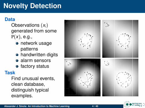
DataObservations (xi)generated from someP(x), e.g.,

network usagepatternshandwritten digitsalarm sensorsfactory status

TaskFind unusual events,clean database,distinguish typicalexamples.


Applications

Network Intrusion DetectionDetect whether someone is trying to hack the network,downloading tons of MP3s, or doing anything else unusualon the network.

Jet Engine Failure DetectionYou can’t destroy jet engines just to see how they fail.

Database CleaningWe want to find out whether someone stored bogusinformation in a database (typos, etc.), mislabelled digits,ugly digits, bad photographs in an electronic album.

Fraud DetectionCredit Cards, Telephone Bills, Medical Records

Self calibrating alarm devicesCar alarms (adjusts itself to where the car is parked), homealarm (furniture, temperature, windows, etc.)


Novelty Detection via Densities

Key IdeaNovel data is one that we don’t see frequently.It must lie in low density regions.

Step 1: Estimate densityObservations x1, . . . , xm

Density estimate via Parzen windowsStep 2: Thresholding the density

Sort data according to density and use it for rejectionPractical implementation: compute

p(xi) =1m

∑j

k(xi , xj) for all i

and sort according to magnitude.Pick smallest p(xi) as novel points.


Typical Data


Outliers


A better way . . .


A better way . . .

ProblemsWe do not care about estimating the density properly inregions of high density (waste of capacity).We only care about the relative density for thresholdingpurposes.We want to eliminate a certain fraction of observationsand tune our estimator specifically for this fraction.

SolutionAreas of low density can be approximated as the levelset of an auxiliary function. No need to estimate p(x)directly — use proxy of p(x).Specifically: find f (x) such that x is novel if f (x) ≤ cwhere c is some constant, i.e. f (x) describes the amountof novelty.


Maximum Distance Hyperplane

Idea Find hyperplane, given by f (x) = 〈w , x〉+ b = 0 that hasmaximum distance from origin yet is still closer to theorigin than the observations.

Hard Margin

minimize12‖w‖2

subject to 〈w , xi〉 ≥ 1

Soft Margin

minimize12‖w‖2 + C

m∑i=1

ξi

subject to 〈w , xi〉 ≥ 1− ξi

ξi ≥ 0Alexander J. Smola: An Introduction to Machine Learning 11 / 40

The ν-Trick

ProblemDepending on C, the number of novel points will vary.We would like to specify the fraction ν beforehand.

SolutionUse hyperplane separating data from the origin

H := {x |〈w , x〉 = ρ}

where the threshold ρ is adaptive.Intuition

Let the hyperplane shift by shifting ρAdjust it such that the ’right’ number of observations isconsidered novel.Do this automatically


The ν-Trick

Primal Problem

minimize12‖w‖2 +

m∑i=1

ξi −mνρ

where 〈w , xi〉 − ρ + ξi ≥ 0ξi ≥ 0

Dual Problem

minimize12

m∑i=1

αiαj〈xi , xj〉

where αi ∈ [0, 1] andm∑

i=1

αi = νm.

Similar to SV classification problem, use standard optimizerfor it.


USPS Digits

Better estimates since we only optimize in low densityregions.Specifically tuned for small number of outliers.Only estimates of a level-set.For ν = 1 we get the Parzen-windows estimator back.


A Simple Online Algorithm

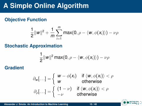
Objective Function

12‖w‖2 +

1m

m∑i=1

max(0, ρ− 〈w , φ(xi)〉)− νρ

Stochastic Approximation

12‖w‖2 max(0, ρ− 〈w , φ(xi)〉)− νρ

Gradient

∂w [. . .] =

{w − φ(xi) if 〈w , φ(xi)〉 < ρw otherwise

∂ρ[. . .] =

{(1− ν) if 〈w , φ(xi)〉 < ρ−ν otherwise


Practical Implementation

Update in coefficients

αj ←(1− η)αj for j 6= i

αi ←{

ηi if∑i−1

j=1 αik(xi , xj) < ρ

0 otherwise

ρ =

{ρ + η(ν − 1) if

∑i−1j=1 αik(xi , xj) < ρ

ρ + ην otherwise

Using learning rate η.


Online Training Run


Worst Training Examples


Worst Test Examples


Mini Summary

Novelty Detection via Density EstimationEstimate density e.g. via Parzen windowsThreshold it at level and pick low-density regions asnovel

Novelty Detection via SVMFind halfspace bounding dataQuadratic programming solutionUse existing tools

Online VersionStochastic gradient descentSimple update rule: keep data if novel, but only withfraction ν and adjust threshold.Easy to implement


A simple problem


Inference

p(weight|height) =p(height, weight)

p(height)∝ p(height, weight)


Bayesian Inference HOWTO

Joint ProbabilityWe have distribution over y and y ′, given training and testdata x , x ′.

Bayes RuleThis gives us the conditional probability via

p(y , y ′|x , x ′) = p(y ′|y , x , x ′)p(y |x) and hencep(y ′|y)∝ p(y , y ′|x , x ′) for fixed y .


Normal Distribution in Rn

Normal Distribution in R

p(x) =1√

2πσ2exp

(− 1

2σ2 (x − µ)2)

Normal Distribution in Rn

p(x) =1√

(2π)n det Σexp

(−1

2(x − µ)>Σ−1(x − µ)

)Parameters

µ ∈ Rn is the mean.Σ ∈ Rn×n is the covariance matrix.Σ has only nonnegative eigenvalues:The variance is of a random variable is never negative.


Gaussian Process Inference

Our ModelWe assume that all yi are related, as given by somecovariance matrix K . More specifically, we assume thatCov(yi , yj) is given by two terms:

A general correlation term, parameterized by k(xi , xj)An additive noise term, parameterized by δijσ

2.Practical Solution

Since y ′|y ∼ N(µ̃, K̃ ), we only need to collect all terms inp(t , t ′) depending on t ′ by matrix inversion, hence

K̃ = Ky ′y ′ − K>yy ′K−1

yy Kyy ′ and µ̃ = µ′ + K>yy ′

[K−1

yy (y − µ)]︸︷︷︸

independent of y ′

Key InsightWe can use this for regression of y ′ given y .


Some Covariance Functions

ObservationAny function k leading to a symmetric matrix withnonnegative eigenvalues is a valid covariance function.

Necessary and sufficient condition (Mercer’s Theorem)k needs to be a nonnegative integral kernel.

Examples of kernels k(x , x ′)

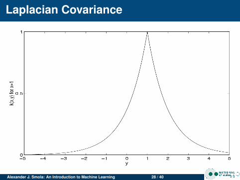
Linear 〈x , x ′〉Laplacian RBF exp (−λ‖x − x ′‖)Gaussian RBF exp

(−λ‖x − x ′‖2)

Polynomial (〈x , x ′〉+ c〉)d, c ≥ 0, d ∈ N

B-Spline B2n+1(x − x ′)Cond. Expectation Ec[p(x |c)p(x ′|c)]


Linear Covariance


Laplacian Covariance


Gaussian Covariance


Polynomial (Order 3)


B3-Spline Covariance


Gaussian Processes and Kernels

Covariance FunctionFunction of two argumentsLeads to matrix with nonnegative eigenvaluesDescribes correlation between pairs of observations

KernelFunction of two argumentsLeads to matrix with nonnegative eigenvaluesSimilarity measure between pairs of observations

Lucky GuessWe suspect that kernels and covariance functions arethe same . . .


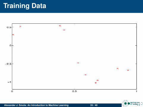
Training Data


Mean ~k>(x)(K + σ21)−1y


Variance k(x , x) + σ2− ~k>(x)(K + σ21)−1~k(x)


Putting everything together . . .


Another Example


The ugly details

Covariance MatricesAdditive noise

K = Kkernel + σ21

Predictive mean and variance

K̃ = Ky ′y ′ − K>yy ′K−1

yy Kyy ′ and µ̃ = K>yy ′K−1

yy y

Pointwise prediction

Kyy = K + σ21

Ky ′y ′ = k(x , x) + σ2

Kyy ′ = (k(x1, x), . . . , k(xm, x))

Plug this into the mean and covariance equations.


Mini Summary

Gaussian ProcessLike function, just randomMean and covariance determine the processCan use it for estimation

RegressionJointly normal modelAdditive noise to deal with error in measurementsEstimate for mean and uncertainty


Support Vector Regression

Loss FunctionGiven y , find f (x) such that the loss l(y , f (x)) is minimized.

Squared loss (y − f (x))2.Absolute loss |y − f (x)|.ε-insensitive loss max(0, |y − f (x)| − ε).Quantile regression lossmax(τ(y − f (x)), (1− τ)(f (x)− y)).

Expansionf (x) = 〈φ(x), w〉+ b

Optimization Problem

minimizew

m∑i=1

l(yi , f (xi)) +λ

2‖w‖2


Regression loss functions


Summary

Novelty DetectionBasic ideaOptimization problemStochastic ApproximationExamples

LMS RegressionAdditive noiseRegularizationExamplesSVM Regression


Documents

An Introduction to Machine Learning - Alex Smolaalex.smola.org/teaching/pune2007/pune_5.pdf · An Introduction to Machine Learning L5: Novelty Detection and Regression Alexander J