Introduction to MatLab 1

www.kbraeuer.de

20. November 2015

An Introduction to MatLab

Contents

1. Starting MatLab ................................................................................................. 3

2. Workspace and m-Files .................................................................................... 4

3. Help..................................................................................................................... 5

4. Vectors and Matrices ........................................................................................ 5

5. Objects ............................................................................................................... 8

6. Plots.................................................................................................................. 10

7. Statistics .......................................................................................................... 13

8. Import and Export of Data .............................................................................. 15

9. Appendix (Plots and Codes) ........................................................................... 17

10. Addition ........................................................................................................ 23

11. Physics: Solution of the time dependent Schrödinger-Equation ............ 25

Introduction to MatLab 3

www.kbraeuer.de

20. November 2015

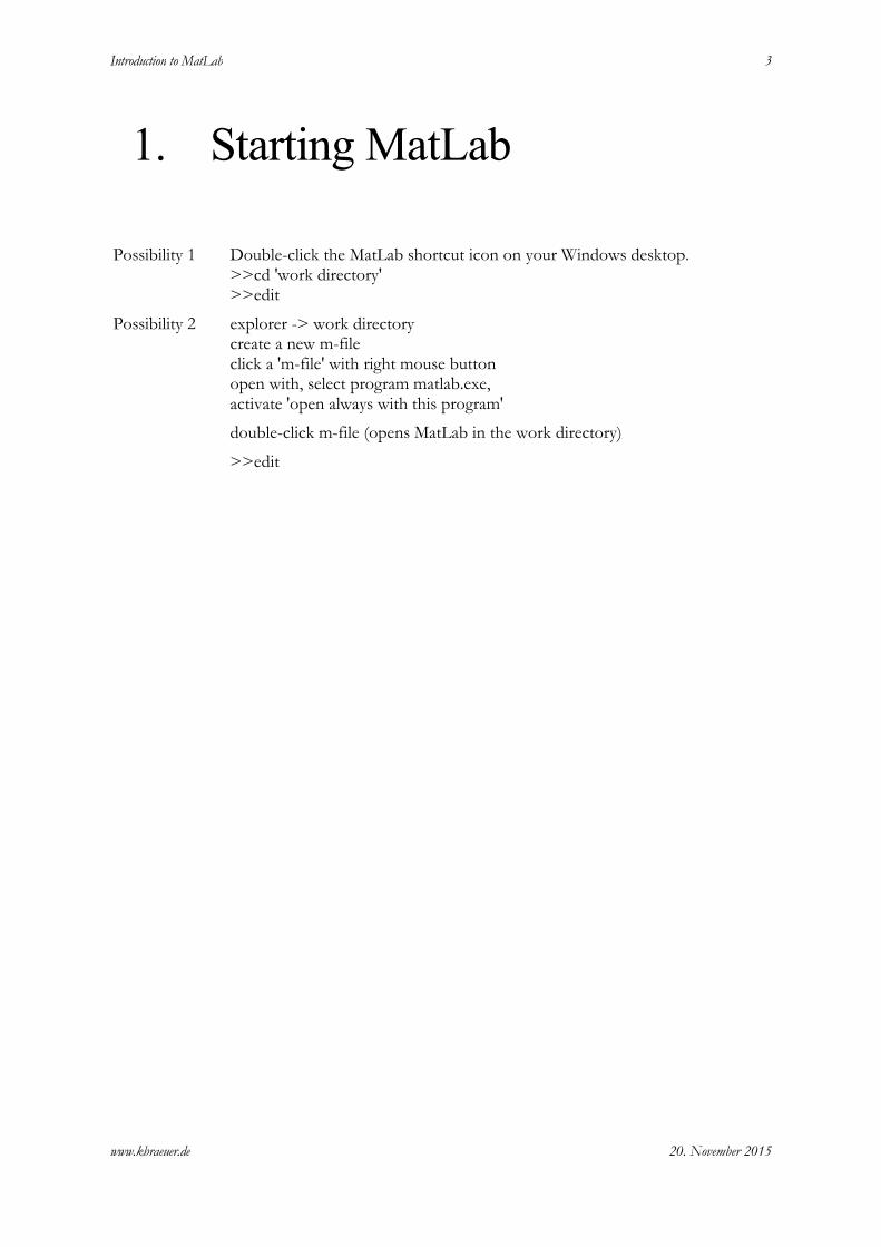
1. Starting MatLab

Possibility 1 Double-click the MatLab shortcut icon on your Windows desktop. >>cd 'work directory' >>edit

Possibility 2 explorer -> work directory create a new m-file click a 'm-file' with right mouse button open with, select program matlab.exe, activate 'open always with this program'

double-click m-file (opens MatLab in the work directory)

>>edit

4

2. Workspace and m-Files

( )

( )( )

5 stores value 5 in variable , prints result in workspace

5

5; stores value 5 in variable

prints value of variable in workspace

5

' ';

' '

a a

a a

a a

t hello world

t

hello world

whos

variable list

>> =

>> =

>>

>>

>> =

>>

>>

( )( )opens editor with m-file

calls function in m-file

edit test test

test test

>>

>>

example: our first MatLab program

' '

5

workspace editor

edit test function test

hello world

F

hello world

>>

Exercise

Open MatLab

Create a new m-file with name 'first'

Type the program lines

( )( )1: 20

,sin * / 5

x

plot x x pi

=

Introduction to MatLab 5

www.kbraeuer.de

20. November 2015

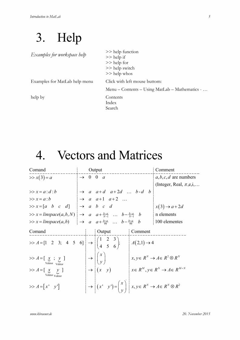
3. Help Examples for workspace help

>> help function >> help if >> help for >> help switch >> help whos

Examples for MatLab help menu

Click with left mouse buttom:

Menu – Contents – Using MatLab – Mathematics - …

help by Contents Index Search

4. Vectors and Matrices

( )

( )1 1

Comand Output Comment

0 0 , , , are numbers 3

(Integer, Real, ,e,i,

: : 2 -

: 1 2

[ ] 3 2

( , , ) n elements

( , )

b a b aN N

a a b c dx a

x a d b a a d a d b d b

x a b a a a

x a b c d a b c d x a d

x linspace a b N a a b b

x linspace a b

π

− −− −

→>> =

>> = → + +

>> = → + +

>> = → → +

>> = → + −

>> = →

…

…

…

…

99 99100 elementesb a b aa a b b− −+ −…

( )

� �

� � ( )

[ ] ( )

2

Vektor Vektor

Vektor Vektor

'

2

Comand Output Comment

1 2 3[1 2 3; 4 5 6] ; 2,1 4

4 5 6

[ ; ] ,

[ ] ,

' ' ' ' ,

N N

M N M N

N N

A A

xA x y x y R A R R

y

A x y x y x R y R A R

xA x y x y x y R A R R

y

+

>> = → →

>> = → ∈ → ∈ ⊗

>> = → ∈ ∈ → ∈

>> = → = ∈ → ∈ ⊗

6

Scalar produkt:

Comand Comment

' ,

' ,

,

N N

n n

n

M N N M

mn n

n

M N N K M K

mn nk

n

x y x y R R R

A x A x R R R R

A B A B R R R R R R

>> ⋅ = →

>> ⋅ = ⊗ →

>> ⋅ = ⊗ ⊗ → ⊗

∑

∑

∑

( )( )

Point produkt:

Comand Comment

. ,

. ,

N N N

n n

M N M N M N

mn mn

x y x y R R R

A B A B R R R R R R

>> ⋅ = →

>> ⋅ = ⊗ ⊗ → ⊗

( )( )( ) ( )( )( )

2

functions:

Comand Comment

.^ 2

sin sin

N N

n

M N M N

mn

x x R R

A A R R R R

>> = →

>> = ⊗ → ⊗

Exercise

a) Which function is evaluated by

( )1:f prod N=

(>>'help prod' shows the definition and examples for 'prod')

b) Study the results of the commands

( )( )

( )( )( )( )( )

( )

6

1: 6, ,1: 1: ;

, 2

6,: , ', ' '

' '

' '

' 1'

N ones

for n N n n n end

N

f prod N

plot N f b

xlabel N

ylabel f

title Test

whos

>> =

>> = =

>>

>> =

>>

>>

>>

>>

>>

c) Use

1 2 3 14

2 3 1 and 11

3 1 2 11

A B

= =

Introduction to MatLab 7

www.kbraeuer.de

20. November 2015

ci) Calculate the determinant of A (Menu help: MatLab - Using MatLab – Matrices and linear algebra – Inverses …)

cii) Solve the linear system Ax B= (Menu help: MatLab - Using MatLab – Matrices and linear algebra – Solving linear…)

d) Consider the commands Comand Output

x=1:5 1 2 3 4 5

y=-2:2 2 -1 0 1 2

z=y>0 z=0 0 0 1 1

x(z) 4 5

x

y

>> =

>> = −

>>

>>

Explain the result in the last line!

(z is a logical array, x(z) maps to the elements of x, for which z is 1)

e) Compare the two codes

( ) ( )

code 1 code 2

5 8 5 8

1: ; 1: ;

0; '

for n=1:N

;

end

y

N e N e

x N x N

y y x x

y y x n x n

= =

= =

= = ⋅

= + ⋅

Consider specially the run time!

8

5. Objects Example

� and

Position

0,0 , 'hello world'x y

hnd text

>> =

>> hnd=text(0,0,'hello world') hnd = 101.0002 >> get(hnd) Color = [0 0 0] EraseMode = normal Editing = off Extent = [-0.00125786 -0.0176056 0.0792453 0.0316901] FontAngle = normal FontName = Helvetica FontSize = [10] FontUnits = points FontWeight = normal HorizontalAlignment = left Position = [0 0 0] Rotation = [0] String = hello world Units = data Interpreter = tex VerticalAlignment = middle BeingDeleted = off ButtonDownFcn = Children = [] Clipping = off CreateFcn = DeleteFcn = BusyAction = queue HandleVisibility = on HitTest = on Interruptible = on Parent = [100.001] Selected = off SelectionHighlight = on Tag = Type = text UIContextMenu = [] UserData = [] Visible = on

Get possibile properties:

( ), 'HorizontalAlignment'

[ {left} | center | right ]

set hnd>>

Set possibile properties: ( ), ' ', ' ', ' ', 25set hnd HorizontalAlignment center FontSize>>

Exercise

a) Rotate the string 'hello world' by 180 degrees (Rotation is a property of the object 'text'.

b) Type in the command [ ] [ ]( )1 0 1 , 0 1 0h plot>> = −

Introduction to MatLab 9

www.kbraeuer.de

20. November 2015

bi) What different line styles are possible

bii) Change the line style and the line width

biii) change the y-data to [0 1 1.5]

10

6. Plots >>help plot

( )( )( )( )

(0,2* );

,sin

,sin , ' : '

x linspace pi

plot x x

plot x x b

>> =

>>

>>

[ ][ ]

( )( ) ( )

( ) ( )( ) ( )

0 1 1 0 ;

.5* 0 0 1 1 ;

, , ' ' or

, , ' ' Hnd is 'handle' for object

shows object properties

, ' ', ' ', ' ',10 changes object properties

x

y

fill x y y

Hnd fill x y y

get Hnd

set Hnd EdgeColor r LineWidth

>> =

>> =

>>

>> =

>>

>>

� � �, ,rows columns PlotNo

subplot n m k

>>

( )( )overdraw

delete old objects when drawing a new one

hold on

hold off

>>

>>

( ) ( ), 1 , delete grafik window 1try delete end>>

Introduction to MatLab 11

www.kbraeuer.de

20. November 2015

Curve fitting

Data:

( ) ( )1 2 1 2N Nx x x x y y y y= → = ⋯

fit:

2.Y a bX cX= + +

get a, b and c with MatLab:\

( )( )�

' 1 ' . ^ 2 '

\ '

*

M

A

a

y x x b

c

A M y

Y M A

=

=

=

=

=

�������

12

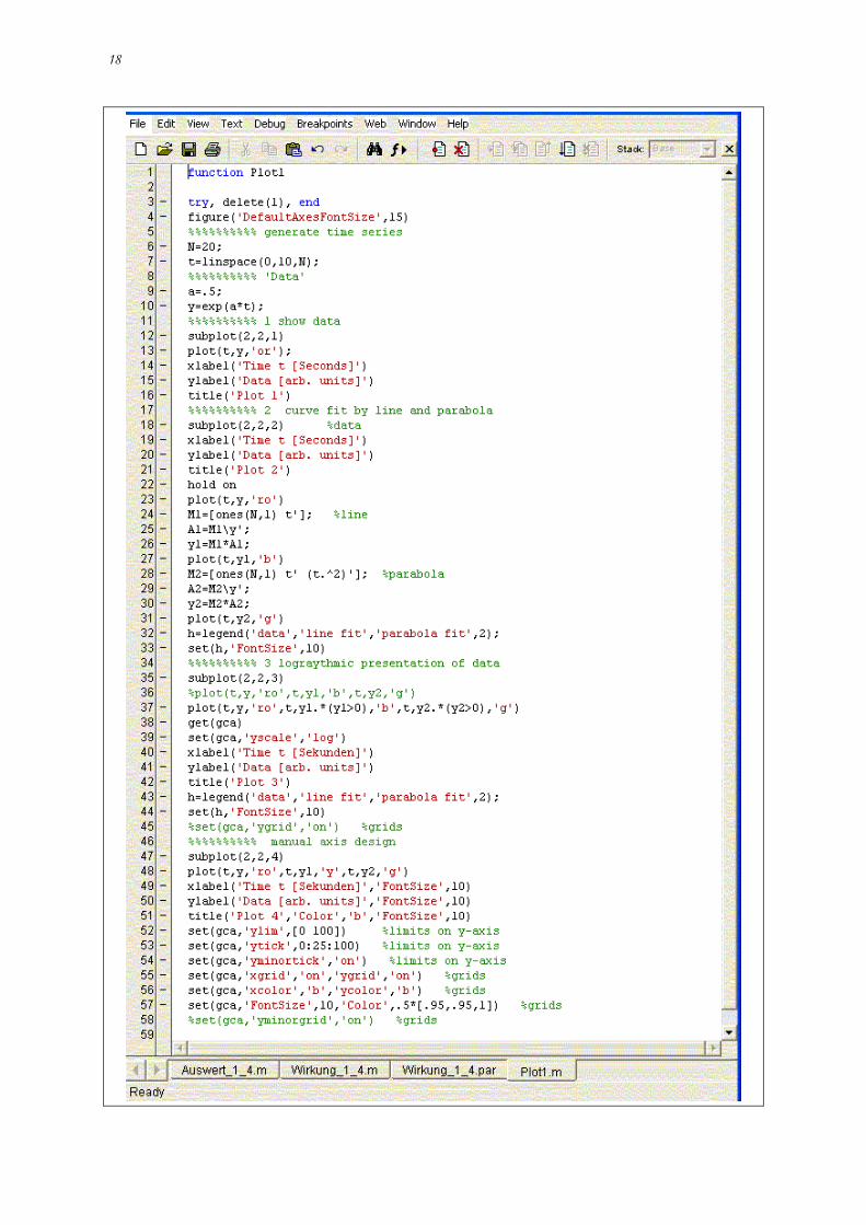
Exercise

Create a new m-file 'Plot1'

Create the time series t=0..10 ,y=exp(at) with N elements;

Reproduce the plots of Plot1 in the appendix

If you don't know how to proceed, look into the program file (after the figure)

Use the desktop help and the help menu to get an understanding of the statements

Introduction to MatLab 13

www.kbraeuer.de

20. November 2015

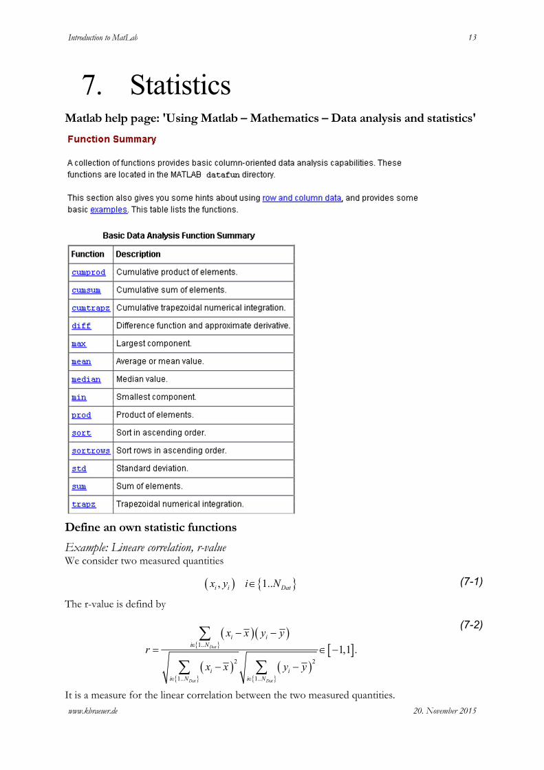
7. Statistics Matlab help page: 'Using Matlab – Mathematics – Data analysis and statistics'

Define an own statistic functions

Example: Lineare correlation, r-value We consider two measured quantities

( ) { }, 1..i i Datx y i N∈ (7-1)

The r-value is defind by

( )( ){ }

( ){ }

( ){ }

[ ]1..

2 2

1.. 1..

1,1 .Dat

Dat Dat

i i

i N

i i

i N i N

x x y y

r

x x y y

∈

∈ ∈

− −

= ∈ −

− −

∑

∑ ∑

(7-2)

It is a measure for the linear correlation between the two measured quantities.

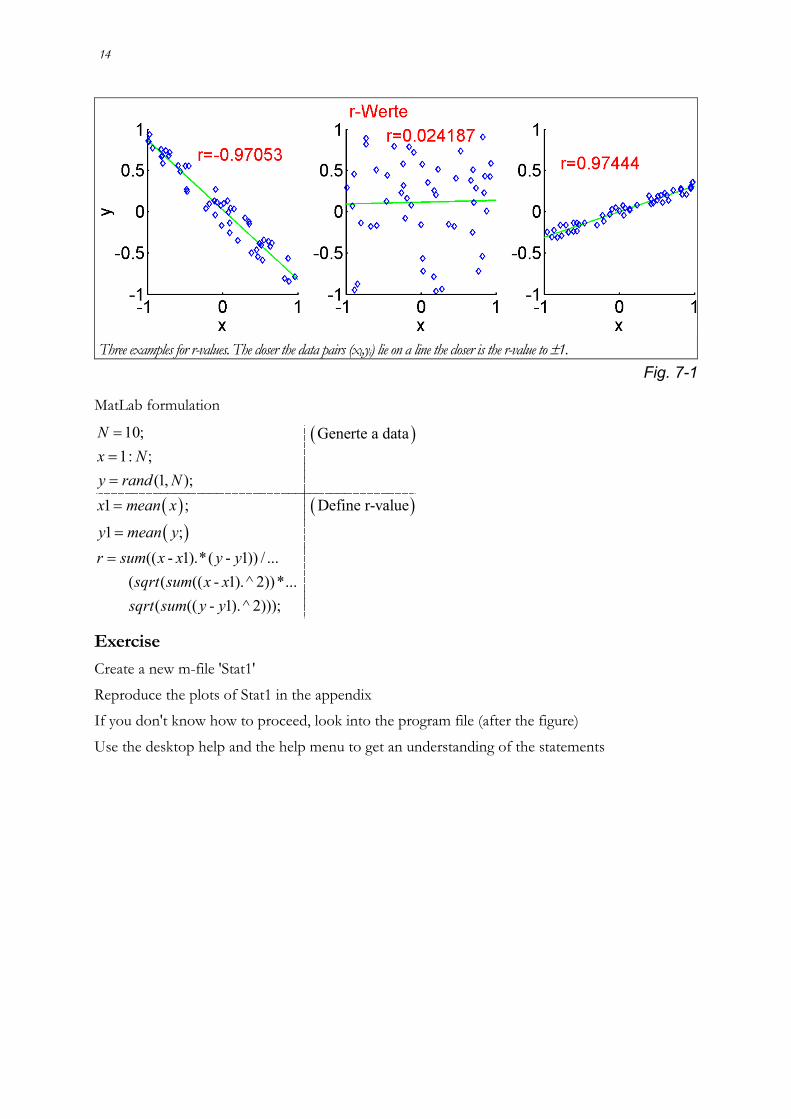
14

Three examples for r-values. The closer the data pairs (xI,yi) lie on a line the closer is the r-value to ±1.

Fig. 7-1

MatLab formulation

( )

( )( )

( )

10; Generte a data

1: ;

(1, );

1 ; Define r-value

1 ;

(( - 1).*( - 1)) / ...

( ( (( - 1).^ 2))*...

( (( - 1).^ 2)));

N

x N

y rand N

x mean x

y mean y

r sum x x y y

sqrt sum x x

sqrt sum y y

=

=

=

=

=

=

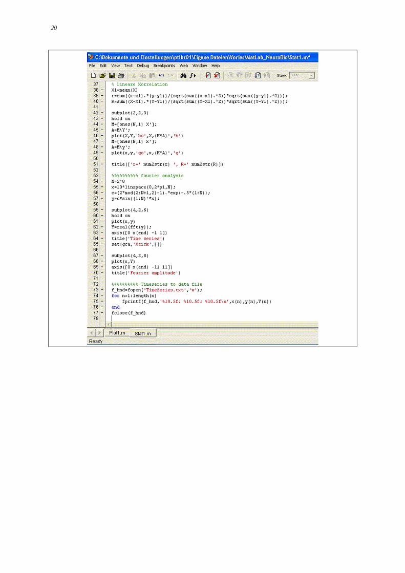
Exercise

Create a new m-file 'Stat1'

Reproduce the plots of Stat1 in the appendix

If you don't know how to proceed, look into the program file (after the figure)

Use the desktop help and the help menu to get an understanding of the statements

Introduction to MatLab 15

www.kbraeuer.de

20. November 2015

8. Import and Export of Data Matlab help: 'Using matlab – Development environment – Importing and ex-porting -

16

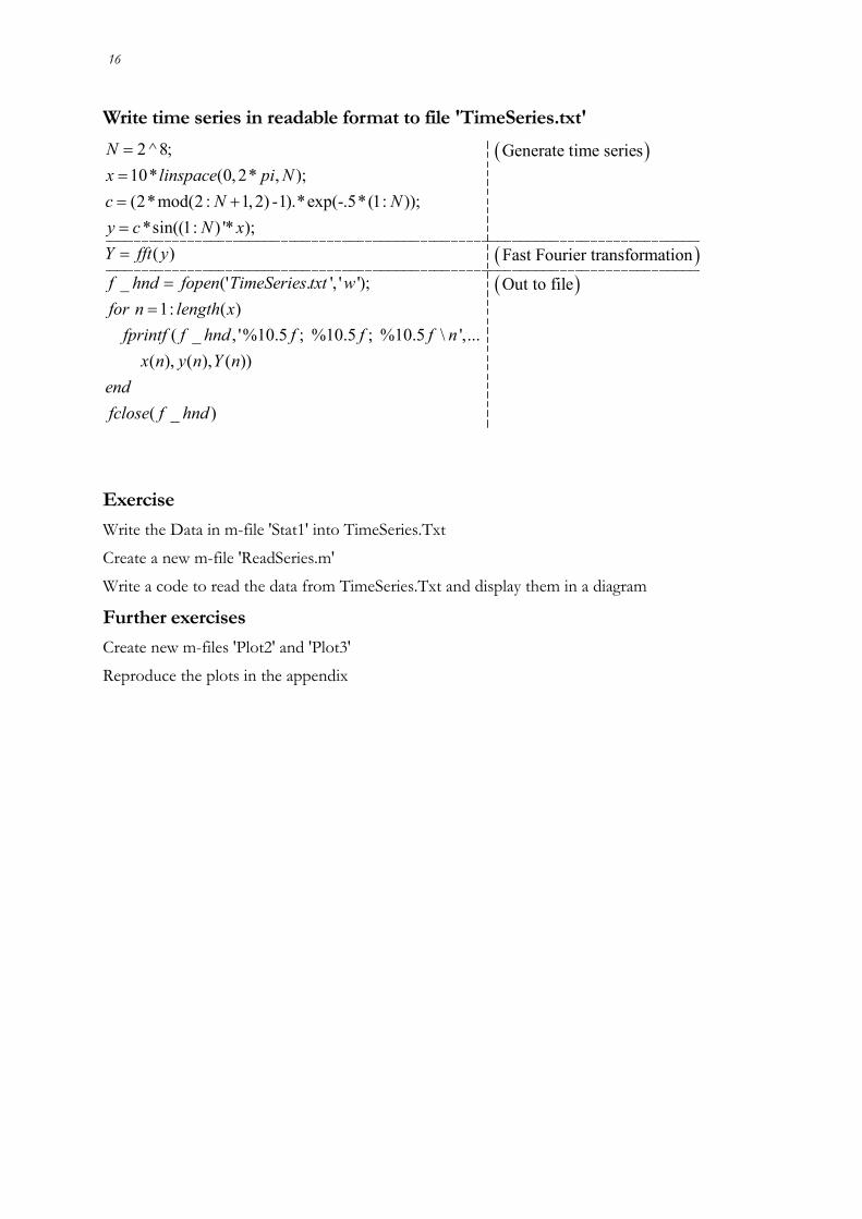
Write time series in readable format to file 'TimeSeries.txt'

( )

( )

2 ^ 8; Generate time series

10* (0, 2* , );

(2*mod(2 : 1, 2) -1).*exp(-.5*(1: ));

*sin((1: ) '* );

( ) Fast Fourier transformation

_ (' . ', ' ');

1: ( )

N

x linspace pi N

c N N

y c N x

Y fft y

f hnd fopen TimeSeries txt w

for n length x

fprin

=

=

= +

=

=

=

=( )Out to file

( _ , '%10.5 ; %10.5 ; %10.5 \ ',...

( ), ( ), ( ))

( _ )

tf f hnd f f f n

x n y n Y n

end

fclose f hnd

Exercise

Write the Data in m-file 'Stat1' into TimeSeries.Txt

Create a new m-file 'ReadSeries.m'

Write a code to read the data from TimeSeries.Txt and display them in a diagram

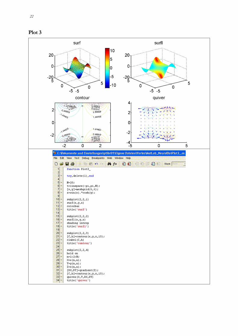
Further exercises

Create new m-files 'Plot2' and 'Plot3'

Reproduce the plots in the appendix

Introduction to MatLab 17

www.kbraeuer.de

20. November 2015

9. Appendix (Plots and Codes) Plot 1

18

Introduction to MatLab 19

www.kbraeuer.de

20. November 2015

Statistics 1

Fortsetzung des Programms

20

Introduction to MatLab 21

www.kbraeuer.de

20. November 2015

Plot 2

22

Plot 3

Introduction to MatLab 23

www.kbraeuer.de

20. November 2015

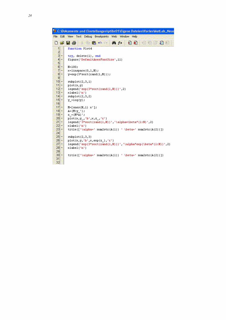
10. Addition Exercise (Fit of arbitrary functions)

Create a 'random exponential function' by

( )( )( )exp 3 sort ran 1:y N= ⋅

Approximate this function by

xz eβα=

Tipp:

Approximate ( ) ( )( ) ( )log by y x y x z x xα β= = +ɶ ɶ . Its an easy way to get α and β. The you can

display xz eβα= .

24

Introduction to MatLab 25

www.kbraeuer.de

20. November 2015

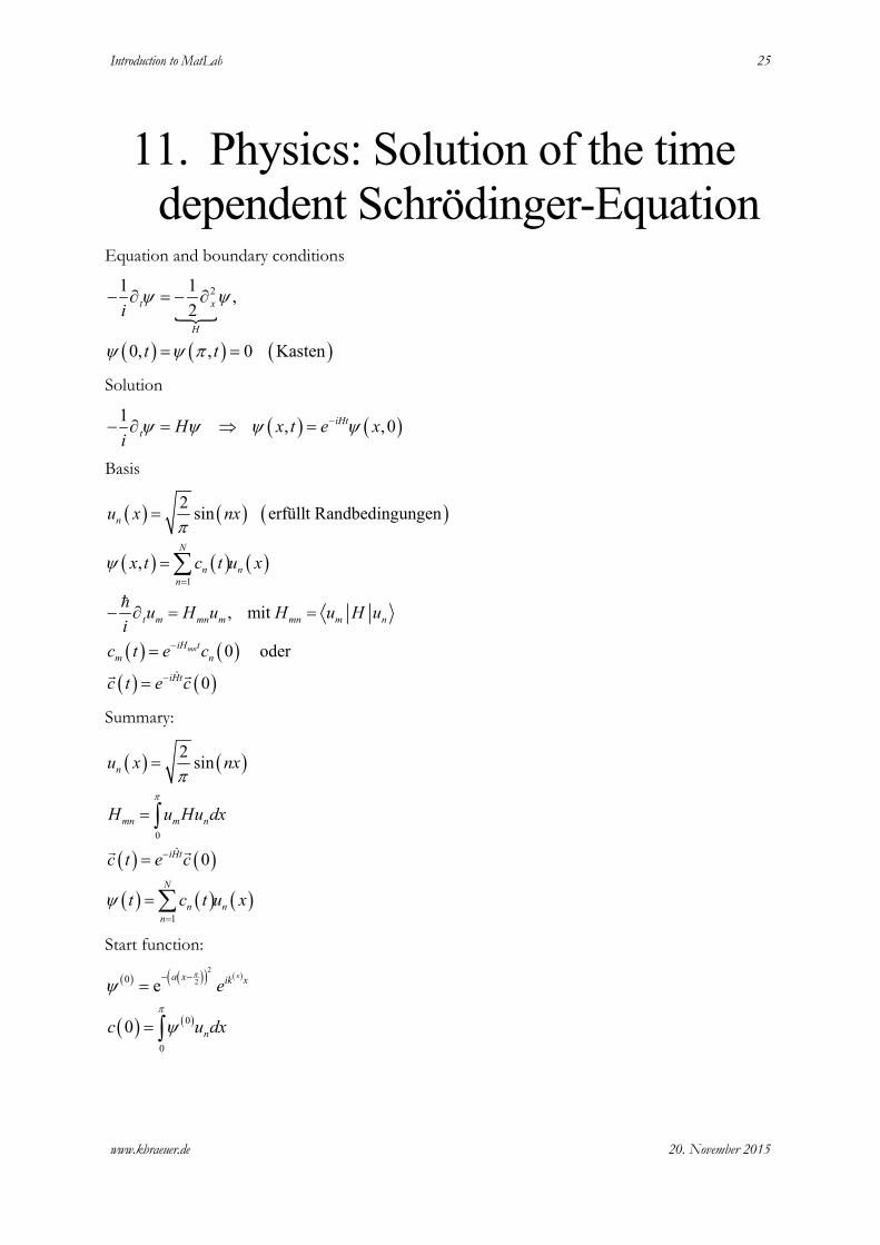
11. Physics: Solution of the time

dependent Schrödinger-Equation Equation and boundary conditions

�

( ) ( ) ( )

21 1,

2

0, , 0 Kasten

t x

H

i

t t

ψ ψ

ψ ψ π

− ∂ = − ∂

= =

Solution

( ) ( )1, ,0iHt

t H x t e xiψ ψ ψ ψ−− ∂ = ⇒ =

Basis

( ) ( ) ( )

( ) ( ) ( )

( ) ( )( ) ( )

1

ˆ

2sin erfüllt Randbedingungen

,

, mit

0 oder

0

mn

n

N

n n

n

t m mn m mn m n

iH t

m n

iHt

u x nx

x t c t u x

u H u H u H ui

c t e c

c t e c

π

ψ=

−

−

=

=

− ∂ = =

=

=

∑ℏ

Summary:

( ) ( )

( ) ( )

( ) ( ) ( )

0

ˆ

1

2sin

0

n

mn m n

iHt

N

n n

n

u x nx

H u Hu dx

c t e c

t c t u x

π

π

ψ

−

=

=

=

=

=

∫

∑

Start function:

( ) ( )( ) ( )

( ) ( )

2

20

0

0

e

0

xa x ik x

n

e

c u dx

π

π

ψ

ψ

− −=

= ∫

26

Formulation with vectors and matrices

( )( ) ( )

( )

0, ,

2 1

1:M

x linspace N

dx x x

f M

π=

= −

=

( ) ( ) ( )( )( ) ( )( )'2 2sin sinn

M M

mx mu u f x n f xπ π= = = ⋅

( ) ( )( ) ( ) ( )

( ) ( ) ( )( )

2 2 2

22 '

0

,1

.

M

nm

mn m n m n

D D m ones N f

H u n u dx u D u dx

π

= = − = − ⋅

= − = ⋅ ⋅∫

( ) ( )( ) ( )( )

( ) ( ) ( ) ( )( ) ( ) ( ) ( )

2

02/0 0

0 ' 0 ' 01

1

.

0

x B ikx

m

N

nm m n

e e

c u dx u dx R R u x x dx

π

ψ ψ

ψ ψ ψ

− −= = ⋅

= = ∈ ⊗

∫≃

Introduction to MatLab 27

www.kbraeuer.de

20. November 2015

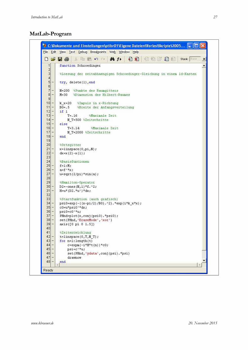
MatLab-Program