An Introduction to Meta-analysis

Douglas G. Bonett

4/10/2016

Overview

• What is a “meta-analysis”?

• Some common measures of effect size

• Three kinds of meta-analysis statistical models

• Combining results from multiple studies

• Converting from one effect-size measure to another

• Comparing results from multiple studies

• Assessing and adjusting for publication bias

What is a “Meta-analysis”

A meta-analysis uses summary information (e.g., sample correlations,

sample means, sample proportions) from m ≥ 2 studies. In each study,

a sample of participants is obtained from some study population and the

sample data are used to estimate a population “effect size” parameter

(e.g., mean difference, standardized mean difference, odds ratio,

correlation, slope coefficients, etc.).

Statistical methods are then used to compare or combine the m effect

size estimates.

Benefits of a Meta-analysis

A comparison of effect size estimates can assess interesting differences

across the m study populations. If a statistical analysis indicates that the

population effect sizes are meaningfully different across the study

populations, certain characteristics of the study populations (length of

treatment, age of participants, etc.) could be due to scientifically

interesting moderator variables. The discovery of a moderator variable

could clarify current theory and suggest new avenues of inquiry.

The m effect size estimates also can be combined to obtain a single,

more precise, estimate of an effect size that generalizes to all m study

populations.

Some Common Effect-size Measures

Pearson correlation (𝜌𝑥𝑦) – describes the strength of a linear relation

between two quantitative variables (x and y)

Point-biserial correlation (𝜌𝑝𝑏) – describes the strength of a relation

between a quantitative variable and a dichotomous variable

Standardized mean difference (𝛿) – describes the mean difference

between treatment conditions (or subpopulations) in standard deviation

units

Odds ratio (𝜔) – describes the strength of relation between two

dichotomous variables

Meta-analysis Statistical Models

Let 𝜃𝑘 present some measure of effect size (correlation, standardized

mean difference, proportion difference, odds ratio, etc.) for study k (k =

1 to m). The estimator of 𝜃𝑘 and its estimated variance will be denoted

as 𝜃𝑘 and var( 𝜃𝑘 ), respectively. 𝜃𝑘 is a random variable and a

statistical model may be used to represent its large-sample expected

value and random deviation from expectation.

Three basic types of statistical models – the constant coefficient

model, the varying coefficient model, and the random coefficient

model – can be used to represent the estimators from multi-study

designs.

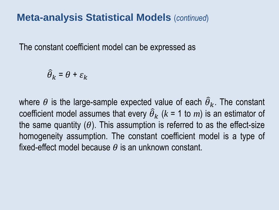
Meta-analysis Statistical Models (continued)

The constant coefficient model can be expressed as

𝜃𝑘 = 𝜃 + 휀𝑘

where 𝜃 is the large-sample expected value of each 𝜃𝑘. The constant

coefficient model assumes that every 𝜃𝑘 (k = 1 to m) is an estimator of

the same quantity (𝜃). This assumption is referred to as the effect-size

homogeneity assumption. The constant coefficient model is a type of

fixed-effect model because 𝜃 is an unknown constant.

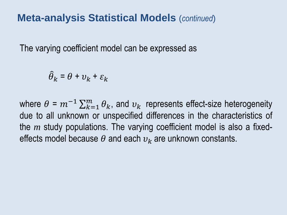
Meta-analysis Statistical Models (continued)

The varying coefficient model can be expressed as

𝜃𝑘 = 𝜃 + 𝜐𝑘 + 휀𝑘

where 𝜃 = 𝑚−1 𝑘=1𝑚 𝜃𝑘, and 𝜐𝑘 represents effect-size heterogeneity

due to all unknown or unspecified differences in the characteristics of

the m study populations. The varying coefficient model is also a fixed-

effects model because 𝜃 and each 𝜐𝑘 are unknown constants.

Meta-analysis Statistical Models (continued)

The random coefficient model can be expressed as

𝜃𝑘 = 𝜃∗+ 𝜐𝑘 + 휀𝑘

where 𝜐𝑘 is assumed to be a normally distributed random variable with

mean 0 and standard deviation 𝜏. To justify the claim that 𝜐𝑘 is a

random variable, two-stage cluster sampling can be assumed. One way

to conceptualize two-stage cluster sampling is to randomly select m

study populations from a superpopulation of M study populations and

then take a random sample of size 𝑛𝑘 from each of the m randomly

selected study populations.

Meta-analysis Statistical Models (continued)

All three models can be used to combine results from m studies to

estimate a single effect size parameter.

constant coefficient (CC) model: 𝜃

varying coefficient (VC) model: 𝑚−1 𝑘=1𝑚 𝜃𝑘

random coefficient (RC) model: 𝜃∗

Limitations of Each Model

In the CC model, the estimate of 𝜃 is biased and inconsistent unless

𝜃1 = 𝜃2 = … = 𝜃𝑚.

In the CC and VC models, the single effect size describes the m study

populations. This can be viewed as a limitation because in the RC

model, 𝜃∗ describes the average of all M > m effect sizes in the

superpopulation.

In the RC model, the estimate of 𝜃∗ is biased and inconsistent if the

variances of 𝜃𝑘 are correlated with 𝜃𝑘 (which is a common situation).

Limitations of Each Model (continued)

The RC model is difficult to justify unless the m studies are assumed tobe a random sample from some definable superpopulation.

A confidence interval for the standard deviation of the superpopulationeffect sizes (𝜏) in the RC model is hypersensitive to minor violations ofthe superpopulation normality assumption.

The confidence interval for 𝑚−1 𝑘=1𝑚 𝜃𝑘 (VC model) is wider than the

confidence interval for 𝜃 (CC model).

Recommendation: The VC model should be used in most casesunless the assumptions of the CC or RC models can be satisfied.

General Confidence Interval for 𝜃 = 𝑚−1 𝑘=1𝑚 𝜃𝑘

An estimate of 𝜃 = 𝑚−1 𝑘=1𝑚 𝜃𝑘 is

𝜃 = 𝑚−1 𝑘=1𝑚 𝜃𝑘

and the estimated variance of 𝜃 is

var( 𝜃) = 𝑚−2 𝑘=1𝑚 𝑣𝑎𝑟( 𝜃𝑘)

and an approximate 100(1 – 𝛼)% confidince interval for 𝜃 is

𝜃 ± 𝑧𝛼/2 var( 𝜃).

Example: Correlations

The Pearson correlations between Beck Depression Inventory (BDI) scoresand drug use was reported in m = 4 different studies. Hypothetical data aregiven below.

Study 𝜌𝑥𝑦 n 95% CI__________________________________

1 .40 55 [.15, .60]2 .65 90 [.51, .76]3 .60 65 [.42, .74]

4 .45 35 [.14, .68]_____________________________Average .53 [.41, .62]

Note that the CI for the average correlation is narrower than any of the single-study CIs. Furthermore, the CI for the average correlation describes all fourstudy populations.

Example: Odds Ratios

Three studies each used a two-group nonexperimental design tocompare adults diagnosed with traumatic brain injury (TBI) with amatched control group that did not have TBA. In each study, theparticipants were asked if they had experienced suicidal thoughts (ST)in the past 30 days (yes or no). Hypothetical data are given below.

TBI No TBI

Study ST No ST ST No ST 𝜔 95% CI ____________________________________________________

1 41 59 22 78 2.43 [1.32, 4.50]2 9 4 8 15 3.85 [0.96, 15.6]3 13 5 22 30 3.33 [1.07, 10.3]

____________________________________________________Average (geometric) 3.14 [1.67, 5.93]

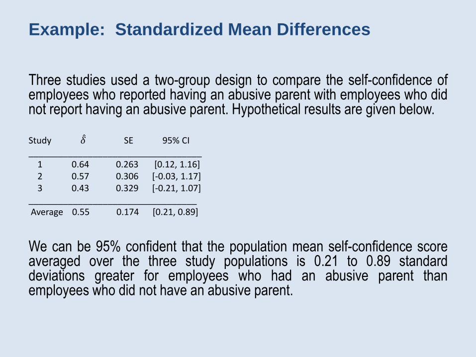
Example: Standardized Mean Differences

Three studies used a two-group design to compare the self-confidence ofemployees who reported having an abusive parent with employees who didnot report having an abusive parent. Hypothetical results are given below.

Study 𝛿 SE 95% CI___________________________________

1 0.64 0.263 [0.12, 1.16]2 0.57 0.306 [-0.03, 1.17]3 0.43 0.329 [-0.21, 1.07]

__________________________________Average 0.55 0.174 [0.21, 0.89]

We can be 95% confident that the population mean self-confidence scoreaveraged over the three study populations is 0.21 to 0.89 standarddeviations greater for employees who had an abusive parent thanemployees who did not have an abusive parent.

Effect-size Conversions

black arrow = exact conversion

blue arrow = approximate conversion

𝜌𝑥𝑦 𝜔 𝛿 𝜌𝑝𝑏

Some Effect-size Conversion Formulas

𝜌𝑝𝑏 =𝛿

𝛿2 +1𝑝𝑞

𝛿 =𝜌𝑝𝑏 1/𝑝𝑞

1 − 𝜌𝑝𝑏2

𝛿 ≈𝑙𝑛 𝜔

1.7𝜔 ≈ 𝑒𝑥𝑝[1.7 𝛿 ]

𝜌𝑥𝑦 ≈𝜔3/4 − 1

𝜔3/4 + 1𝜔 ≈ [

1 + 𝜌𝑥𝑦

1 − 𝜌𝑥𝑦]4/3

𝜌𝑝𝑏 ≈𝑙𝑛 𝜔

𝑙𝑛 𝜔 2 +2.89

𝑝𝑞

𝜔 ≈ 𝑒𝑥𝑝𝜌𝑝𝑏

2.89

𝑝𝑞

1 − 𝜌𝑝𝑏2

where p = 𝑛1/(𝑛1 + 𝑛2) and q = 1 – p

𝜌𝑥𝑦 ≈ (𝜌𝑝𝑏/ℎ) 𝑝𝑞 𝜌𝑝𝑏 ≈ 𝜌𝑥𝑦(ℎ)/ 𝑝𝑞 where h = exp(-𝑧2/2)/2.51 and z is point

on standard unit normal curve that is

exceeded with probability p.

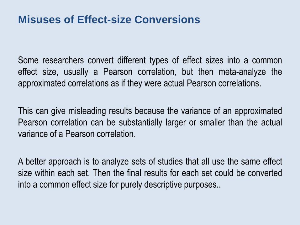
Misuses of Effect-size Conversions

Some researchers convert different types of effect sizes into a common

effect size, usually a Pearson correlation, but then meta-analyze the

approximated correlations as if they were actual Pearson correlations.

This can give misleading results because the variance of an approximated

Pearson correlation can be substantially larger or smaller than the actual

variance of a Pearson correlation.

A better approach is to analyze sets of studies that all use the same effect

size within each set. Then the final results for each set could be converted

into a common effect size for purely descriptive purposes..

Assessing Moderator Effects

A variable that influences the value of an effect-size parameter is called

a moderator variable. Moderator variables can be assessed using a

linear statistical model. The m estimators, 𝜃1, 𝜃2, …, 𝜃𝑚 can be

represented by the following VC linear model

𝜽 = 𝐗𝜷 + 𝐙𝝃 + 𝜺

where X is a design matrix that codes known quantitative or qualitative

characteristics of the m study populations, Z is a matrix of unknown or

unspecified predictor variables.

Estimate of 𝜷

An ordinary least squares estimator of 𝜷 is

𝜷 = (𝐗′𝐗)−1𝐗′ 𝜽

with an estimated covariance matrix

𝑐𝑜𝑣( 𝜷) = (𝐗′𝐗)−1𝐗′ 𝐕𝐗(𝐗′𝐗)−1

where 𝐕 is a diagonal matrix with 𝑣𝑎𝑟( 𝜃𝑘) in the kth diagonal element.

Confidence interval for 𝜷

The estimated variance of 𝛽𝑡 is the tth diagonal element of 𝑐𝑜𝑣( 𝜷)

which will be denoted as 𝑣𝑎𝑟( 𝛽𝑡).

An approximate 100 1 − 𝛼 % confidence interval for 𝛽𝑡 is

𝛽𝑡 ± 𝑧𝛼/2 𝑣𝑎𝑟( 𝛽𝑡) .

Example – Linear Model

Five studies examined the relation between job performance andamount of college education (bachelor vs masters). Average employeetenure in each study varied from 2.1 years to 15.8 years across the fivestudies. The researcher believes that the relation between jobperformance and the amount of college education is moderated bytenure. Hypothetical results are given below.

Study Ave Tenure 𝛿 SE

_________________________________ 𝛽1 = .123 95% CI = [0.011, 0.018]1 2.1 0.68 0.142

2 4.7 0.51 0.093 We are 95% confident that each

3 9.2 0.34 0.159 additional year is associated with a

4 10.7 0.20 0.078 0.011 to 0.018 reduction in 𝛿5 15.8 0.15 0.201

_________________________________

Publication Bias

Effect size estimates from studies with small sample sizes are more

likely to be the result of large anomalous sampling errors that have

exaggerated the effect size and small p-values, and a meta-analysis

that includes these studies will produce biased results. This type of bias

is often referred to as publication bias.

To implement the proposed approach, fit a linear model with an

additional predictor variable (𝑥𝑡) that is equal to 𝑛𝑘∗ − 𝑚𝑖𝑛 𝑛𝑘

∗

where 𝑛𝑘∗ = 1/𝑛𝑘 for 1-group designs and 𝑛𝑘

∗ = 1/𝑛1𝑘 + 1/𝑛2𝑘 for

2-group designs in study k.

Example: Publication Bias

Six different studies examined the correlation between alcohol use andage among 21 to 35 year old adults. The six studies sampled fromsimilar study populations and there were no obvious moderatorvariables to include in the analysis. The sample correlations and samplesizes are given below.

Study n 𝜌𝑥𝑦 1/𝑛𝑘 − 𝑚𝑖𝑛( 1/𝑛𝑘)

__________________________________________ 1 52 -.591 0.077 2 98 -.383 0.0393 76 -.399 0.053 4 159 -.347 0.017 5 258 -.308 0 6 60 -.477 0.067

__________________________________________

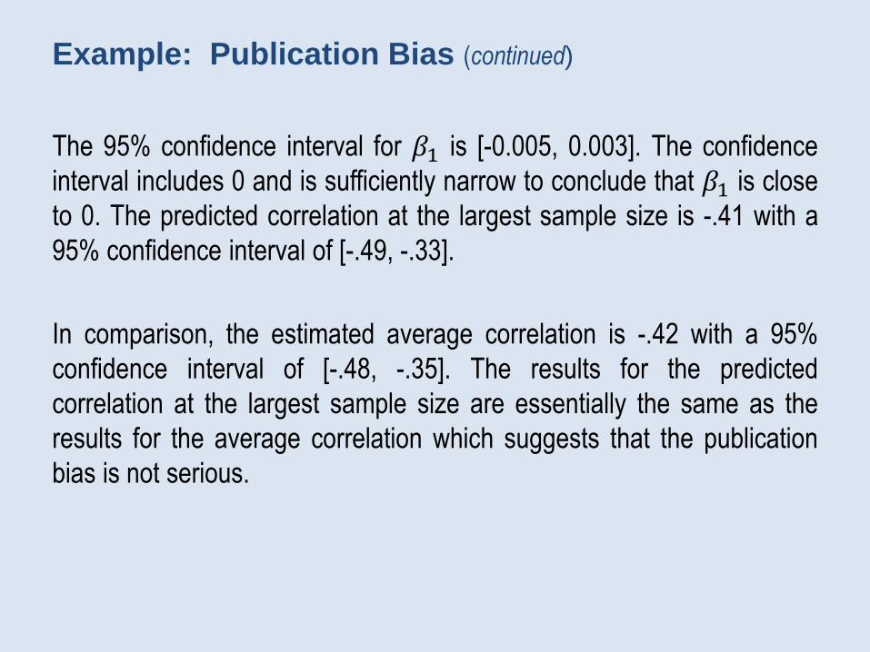
Example: Publication Bias (continued)

The 95% confidence interval for 𝛽1 is [-0.005, 0.003]. The confidence

interval includes 0 and is sufficiently narrow to conclude that 𝛽1 is close

to 0. The predicted correlation at the largest sample size is -.41 with a

95% confidence interval of [-.49, -.33].

In comparison, the estimated average correlation is -.42 with a 95%

confidence interval of [-.48, -.35]. The results for the predicted

correlation at the largest sample size are essentially the same as the

results for the average correlation which suggests that the publication

bias is not serious.

Linear Contrasts

A linear contrast can be expressed as 𝑐1𝜃1 + 𝑐2𝜃2 + ⋯ + 𝑐𝑚𝜃𝑚 where 𝑐𝑘is called a contrast coefficient. A linear contrast can be expressed moreconcisely using summation notation as 𝑘=1

𝑚 𝑐𝑘𝜃𝑘.

For instance, suppose two studies used military samples and three studiesused civilian samples. To assess the possible moderating effect of military vs.civilian, we could estimate

(𝜃1 + 𝜃2)/2 − (𝜃3 + 𝜃4 + 𝜃5)/3

Linear contrasts are especially useful when comparing group means orproportions from two or more studies.

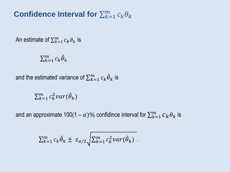
Confidence Interval for 𝑘=1𝑚 𝑐𝑘𝜃𝑘

An estimate of 𝑘=1𝑚 𝑐𝑘𝜃𝑘 is

𝑘=1𝑚 𝑐𝑘

𝜃𝑘

and the estimated variance of 𝑘=1𝑚 𝑐𝑘

𝜃𝑘 is

𝑘=1𝑚 𝑐𝑘

2𝑣𝑎𝑟( 𝜃𝑘)

and an approximate 100(1 – 𝛼)% confidince interval for 𝑘=1𝑚 𝑐𝑘𝜃𝑘 is

𝑘=1𝑚 𝑐𝑘

𝜃𝑘 ± 𝑧𝛼/2 𝑘=1𝑚 𝑐𝑘

2𝑣𝑎𝑟( 𝜃𝑘) .

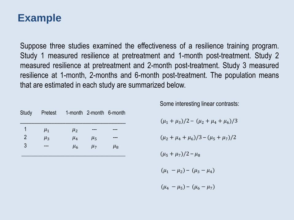
Example

Suppose three studies examined the effectiveness of a resilience training program.

Study 1 measured resilience at pretreatment and 1-month post-treatment. Study 2

measured resilience at pretreatment and 2-month post-treatment. Study 3 measured

resilience at 1-month, 2-months and 6-month post-treatment. The population means

that are estimated in each study are summarized below.

Some interesting linear contrasts:

Study Pretest 1-month 2-month 6-month

_____________________________________ (𝜇1 + 𝜇3)/2 – (𝜇2 + 𝜇4 + 𝜇6)/3

1 𝜇1 𝜇2 --- ---

2 𝜇3 𝜇4 𝜇5 --- (𝜇2 + 𝜇4 + 𝜇6)/3 – (𝜇5 + 𝜇7)/2

3 --- 𝜇6 𝜇7 𝜇8

________________________________________ (𝜇5 + 𝜇7)/2 – 𝜇8

(𝜇1 − 𝜇2) – (𝜇3 − 𝜇4)

(𝜇4 − 𝜇5) – (𝜇6 − 𝜇7)

Some References

Suggested reference texts

Borenstein, M., Hedges, L.V., Higgins, J.P.T. & Rothstein, H.R. (2009) Introduction to meta-analysis. New York: Wiley.

Cooper, H., Hedges, L.V., Valentine, J.C. (2009) The Handbook of research synthesis and meta-analysis, 2nd ed. New York: Russell

Sage Foundation.

References for varying coefficient methods

Bonett, DG (2008) Meta-analytic interval estimation for bivariate correlations. Psychological Methods, 13, 173-189.

Bonett, DG (2009) Meta-analytic interval estimation for standardized and unstandardized mean differences. Psychological

Methods, 14, 225-238.

Bonett, DG (2010) Varying coefficient meta-analytic methods for alpha reliability. Psychological Methods, 15, 368-385.

Bonett, DG & Price RM (2014) Meta-analysis methods for risk differences. British Journal of Mathematical and Statistical

Psychology, 67, 371-389.

Bonett, DG & Price, RM (2015) Varying coefficient meta-analysis methods for odds ratios and risk ratios. Psychological Methods,

20, 394-406.

Questions or comments?