Embed Size (px)
Citation preview

An Introduction to Multi-Valued Model Checking
Georgios E. Fainekos
Department of CIS
University of Pennsylvania
http://www.seas.upenn.edu/~fainekos
Written Preliminary Examination II30th of June, 2005

Model Checking:Is the system correct??
a¬b
¬ab
ab
s0
s2
s1
Extract modelExtract modelFormalizeFormalize
SpecificationSpecification
A[Ga⇒(Xb∨¬a)]
Model Checker Model Checker
YESWitness
NOCounter Example

a=Tb=F
a=Tb=M
a=Mb=T
s0
s2
s1
T
M
TM
T
Multi-Valued Model Checking:In what “degree” is the system correct??
Extract modelExtract modelFormalizeFormalize
SpecificationSpecification
A[Ga⇒(Xb∨¬a)]
MV-Model Checker MV-Model Checker
The “degree” of satisfaction

Why multi-valued model checking?Application 1: conflicting viewpoints
a=TTb=FF
a=FTb=FT
a=FFb=TF
s0
s1
s2
FT
TTTF
TT
Example modified from Chechik et al
a=Tb=F
a=Fb=F
a=Fb=T
s0
s1
s2
a=Tb=F
a=Tb=T
a=Fb=F
s0
s1
s2
FF
TF
TT
FT{ }
{ }
{s1}
{s0,s2}
kEGak
FF
TF
TT
FT{ }
{s0}
{ }
{s1,s2}
kEXbk
FF
TF
TT
FT

Why multi-valued model checking?Application 2: Abstraction
Using 3-valued logicintroduce new special value Maybe to stand for “unknown”
Advantages:No spurious counter-examples
result = T, F or M (unknown)Verification even using incomplete models
p¬qr
pq¬r
¬p¬qr
s0 s1
s2
s0,1 s2
T
M
Tp=Mq=Fr=T
p=Tq=Tr=F
Example taken from Marsha Chechik
F
M
T

{p, ¬p, true}
{¬p, true}{p, true}
{true}{}
{false, p, ¬p, true}
Why multi-valued model checking?Application 3: Query Checking [Chan, CAV’00]
Goal: speed-up design understandingdiscover properties not known a priori
Temporal logic querytemporal logic formula with placeholders (unknowns)
e.g., AG ?x, AG (p → ?x)evaluates to strongest propositional formula that makes query true.
Some applicationsprovide partial explanation when property holds
e.g. instead of AG (a ∨ b), ask AG ?x{a, b}answer a ∧ b is stronger!
provide diagnostic information when property failse.g. if AG (req → AF ack) fails - ask AG (req → AF ?x)
Slide courtesy of Marsha Chechik

Ordering objects
A partial-order is a binary relation ⊑ such that for all x,y,z∈S the following properties hold:
ReflexivityTransitivityAntisymmetry
A poset is the pair: S=(S,⊑)In a linear order all the elements are comparable.
Let X,Y be posets, then a map f : X→Y is called order-preserving if:
x v x
x v y and y v z imply x v z
x v y and y v x imply x = z
(∀x1, x2 ∈ X).(x1 vX x2 → f(x1) vY f(x2))f
top (T)
bottom (⊥)
X
sup(X)
inf(X)

LatticesDefine join ⊔ and meet ⊓ as:
Lattice ℒ is a poset (L,⊑) where for all x,y∈L, x⊓y and x⊔y exist
Complete lattice is a lattice where for all X⊆L, ⊓X and ⊔X exist
c-complete lattice is a complete lattice with complement operator ~ such that ~T=⊥ and ~⊥=T
A lattice is distributive iff it satisfies the distributive law
Let X,Y be posets, then a map f : X→Y is called continuous function if for all non-empty directed sets Z⊆X:
x t y := sup({x, y}) and x u y := inf({x, y})
(∀x, y, z ∈ L).(x u (y t z) = (x u y) t (x u z))
t f(Z) = f(t Z) and u f(Z) = f(t Z)

Some important lemmas
The join and meet are order preserving functions, i.e. for all x,y,z,w∈L
The connecting lemma, for x,y∈L
Every finite lattice is complete
Every continuous function is order preservingIf X,Y are finite posets and f:X→Y is order preserving, then f is continuous
x v y and z v w imply x t z v y t w
x v y iff x t y = y iff x u y = x
x
y w
z

Join irreducible elements
An element x of a lattice ℒ is join irreducible if (i) x≠⊥(ii) x=y⊔z implies x=y or x=z for all y,z∈L
Every element of lattice L can be written as a join of join irreducible elements, for all x∈L:
If L is distributive lattice then, the following are equivalent:
x is join-irreducibleif y,z∈L and x⊑y⊔z then x⊑y or x⊑z
x =F{y ∈ J(L) | y v x}

Quasi-Boolean and Boolean Algebras
• A quasi-Boolean algebra B is a structure B=(B,⊓,⊔, ~,⊥,T); where T and ⊥ are the greatest and least elements, (B,⊓,⊔) is a distributive lattice and ~ is an unary operation of period 2 s.t. for every x∈B there exists unique ~x∈B satisfying:
De Morgan laws:Antimonotonic: Involution: ~~x=x
• A Boolean algebra B is a quasi-Boolean algebra where for each element x∈B the following hold:
Law of non-contradictionLaw of excluded middle
ø (x u y) =ø x tø y ø (x t y) =ø x uø y
x v y iff ø y vø x
x uø x =⊥x tø x = >

Quasi-Boolean and Boolean Algebras (examples)Boolean Algebras
{a,b}
{c}{b}
{a,c}
{a}
{ }
{b,c}
{a,b,c}
B2=({0,1},≤)
BS=(2S,⊆), S={a,b,c}B3=({0,½,1},≤) B3,3=B3×B3
Quasi-Boolean Algebras
0
½
1 true
maybe
false
00
10
11
01
B2,2=B2×B2
0
1 true
false
00
½0
½½
0½
11
10
1½ ½1
01
~1=0, ~0=1, ~½=½
B4+2
0½,½0
½½
1½,½1
10,01
00
11
false
unlikely
disputed
likely
unknown
true

Tarski-Knaster Fixpoint Theorem
• Let L be a complete lattice and f : L → L be an order-preserving function, then f has fixpoints, i.e. f(x) = x. The least and greatest fixpoints are characterized as follows:
• Let y, z in L such that y⊑f(y), y⊑µx.f(x), f(z)⊑z, νx.f(x)⊑z and, let f to be continuous, then the iteration:

Multi-valued sets and relations
• A multi-valued set is a total function from the objects of a set Sto the elements of a lattice ℒ, i.e. : S → L
Intuitively, expresses the “degree” that an object s belongs to a set SActually, in the two-valued case, i.e. when ℒ=B2, it reduces to the characteristic function of the set S
• A multi-valued relation on sets S and T over a lattice L is a function : S × T → L.

An mv Kripke structure is a tuple M = (S, S0, , AP, , ℒ,D)S is a (finite) set of statesS0 is a set of initial states (S0 ⊆S) : S×S → L is an mv-transition relation
AP is a (finite) set of atomic propositions : S×AP → L is a total labelling function that maps a pair of a state s and an atomic proposition a to an element of the lattice Lℒ is a lattice or an algebraD is the set of designated values
mv-Kripke Structures

mv-Kripke Structures (Examples)
Examples courtesy of Marsha Chechik
a=TTb=FF
a=FTb=FT
a=FFb=TF
s0
s1
s2
FT
TTTF
TTpressed = Trequest = F
pressed = Trequest = F
pressed = Mrequest = T
T
T M
T
FF
TF
TT
FT
F
M
T

Predecessor mv-sets
• The existential predecessor set:
• The universal predecessor set:Bruns & Godefroid and Chechik et. al.
Konikowska & Penczek
• Compare with classical definition:
(def. 1)
(def. 2)

Example
a=TTb=FF
a=FTb=FT
a=FFb=TF
s0
s1
s2
FT
TTTF
TT• For any a∈AP, we denote by DaD : S→L the mv-set that represents the “degree”that the proposition a is satisfied in some state s
• The mv-set DaD introduces a partition of the state space
DaD {s0}
{s2}{ }
{s1}
DbD { }
{s1}
{s0}
{s2}
{s0}
{s2}
{ }
{s1}
DbD
Example from Chechik et al
FF
TF
TT
FT
{(s1,s2), (s2,s2)}{(s0,s2)}{(s0,s1)}
{(s0,s0), (s1,s0), (s1,s1),(s2,s0), (s2,s1)}

a=TTb=FF
a=FTb=FT
a=FFb=TF
s0
s1
s2
FT
TTTF
TT
DaD {s0}
{s2}{ }
{s1}
DbD { }
{s1}
{s0}
{s2}
{s0}
{s2}
{ }
{s1}
DbD
Example from Chechik et al
FF
TF
TT
FT
a=Tb=F
a=Fb=F
a=Fb=T
s0
s1
s2
a=Tb=F
a=Tb=T
a=Fb=F
s0
s1
s2
{(s1,s2), (s2,s2)}{(s0,s2)}{(s0,s1)}
{(s0,s0), (s1,s0), (s1,s1),(s2,s0), (s2,s1)}
{ }
{ }
{ }
{s0,s1,s2}
pre∀(DaD) = pre∃(DaD) pre∃(DbD){s0}
{ }
{ }
{s1,s2}

The multi-valued model checking problem
MultiMulti--valued model checking problemvalued model checking problem
(∀s ∈ S0).(kϕkM(s) ∈ D)
Given multi-valued system M = (S, S0, , AP, , ℒ,D) and a specification φ
Alternative:
Given multi-valued system M = (S, S0, , AP, , ℒ,D), state s in S and specification φ determine DφDM(s)

The multi-valued model checking problemTwo main approaches
Reduction methods to classical model checking
Direct methods[Bruns and Godefroid] Extended alternating automata[Chechik et. Al.] Multi-valued CTL symbolic model checking
[Bruns and Godefroid] Reduction for multi-valued µ-calculus[Chechik et. Al.] Reductions for multi-valued LTL, µ-calculus[Konikowska and Penczek] Reduction methods for
mv-CTL* using designated valuesmv-CTL* for FLO and specific lattices (L2,2,L4+2,etc)µ-calculus

Temporal Logics (1)
CTL* syntax
Derived operators

Temporal logics (2):Semantic Intuition of Linear time properties
G a - always a
F a – eventually a
X a – next state a
a U b – a until b
a B b – a before b
a a a a aa
* * a * **
a * * * **
a a b * *a
* a * b **

Temporal Logics (3):Semantic intuition of branching temporal properties

Mv-CTL* model checking using designated values (1)
Semantics of mv-CTL* in Negation Normal Form (NNF)
State formulas
Path formulas

Mv-CTL* model checking using designated values (2)
Theorem 1 (Reduction from NNF mv-CTL* to CTL* using Designated Values) Assume that L is a c-complete lattice.
Let the designated values D and non-designated values N be closed under arbitrary bounds. Define τ : M = (S, S0, , AP+, , ℒ,D) → K = (S, S0, R, AP+, O)
such that:
Then for any state formula φs and any path formula φp of NNF mv-CTL* over the lattice L and any state s in S and path π in PathsM(s) of M, we have:

Sketch of proof:Notice that the paths on M and K are the sameFor any subset LS of L the following properties hold:
Proof proceeds by induction on the structure of φ, some cases:φ=a, a in AP+, then holds by definitionφ=φ1∨φ2, then DφDM(s)=Dφ1DM(s)⊔Dφ2DM(s)∈D iff (property 1) (∃i). (DφiDM(s)∈D) iff (IH) (K,s)⊨φi implies (K,s)⊨φ1∨φ2=φφ=[φ1Uφ2], then DφDM(π[i])∈D iff (property 1) there exists j>i+1 s.t. ((π(j-1), π(j))⊓Dφ2DM(π[j]))∈D iff (as (π(j-1), π(j))∈D and D is closed under bounds) Dφ2DM(π[j])∈D and (property 2) for all 0<k<j ((π(k-1), π(k))⊓Dφ1DM(π[k]))∈D iff Dφ1DM(π[k])∈D iff (IH) on the same path π, (K,π[j])⊨φ2 and for all 0<k<j (K,π[k])⊨φ1 which by definition is (K,π[0])⊨[φ1Uφ2]=φ
Mv-CTL* model checking using designated values (3)

Mv-CTL* model checking using designated values (4)Theorem 2 (Reduction from mv-CTL* to CTL* using Designated Values) Assume that L is a c-complete lattice.
Let the designated values D and non-designated values N be closed under arbitrary bounds.x∈D implies ~x∈N and x∈N implies ~x∈DDefine τ : M = (S, S0, , AP, , ℒ,D) → K = (S, S0, R, AP, O)
such that:
Then for any state formula φs and any path formula φp of NNF mv-CTL* over the lattice L and any state s in S and path π in PathsM(s) of M, we have:
Proof: The only additional case is for the complementation

Examples:• Theorem 1: The condition that D and N should be closed
under arbitrary bounds is satisfied by logics over finite linear orders
i.e. 3-valued Kleene logic, many-value Lukasiewicz logics etc• Theorem 2: The conditions are satisfied by:
Logics over finite linear ordersLogic over the lattice L2,2
Mv-CTL* model checking using designated values (5)
D
N
F
T
~
F
T
D
N
Rosser-Turquette
F
T
D
N
Gödel
F
T
D
N
Lukasiewicz
00
10
11
01
D
N

RemarksThe complexity of mv-CTL* model checking is the same as the two-valued caseThe complexity of CTL* model checking is O(|K|×2|φ|)
A combination of LTL and CTL model checking algorithmsDue to the construction a counter-example in K is a counter-example in MThe approach is helpful as long as we do not care about the exact valueIf the conditions of theorem 2 are satisfied then the 2 definitions of the predecessor sets coincide for the designated values
Mv-CTL* model checking using designated values (6)

The propositional two-valued µ-calculus
Syntax
Semantics

mv-µ-Calculus Model Checking by Reduction (1)
Semantics of mv-µ-calculus in NNF wrt to mv-model MAtomic propositions and mv-transition relation take values over a quasi-Boolean algebra B
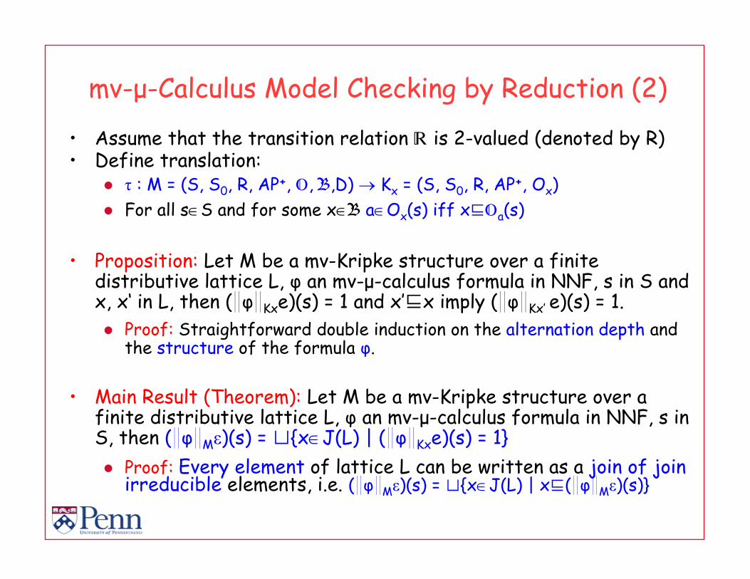
mv-µ-Calculus Model Checking by Reduction (2)
• Assume that the transition relation is 2-valued (denoted by R)• Define translation:
τ : M = (S, S0, R, AP+, , B,D) → Kx = (S, S0, R, AP+, Ox)For all s∈S and for some x∈B a∈Ox(s) iff x⊑a(s)
• Proposition: Let M be a mv-Kripke structure over a finite distributive lattice L, φ an mv-µ-calculus formula in NNF, s in S and x, x‘ in L, then (DφDKxe)(s) = 1 and x’⊑x imply (DφDKx’ e)(s) = 1.
Proof: Straightforward double induction on the alternation depth and the structure of the formula φ.
• Main Result (Theorem): Let M be a mv-Kripke structure over a finite distributive lattice L, φ an mv-µ-calculus formula in NNF, s in S, then (DφDMε)(s) = ⊔{x∈J(L) | (DφDKxe)(s) = 1}
Proof: Every element of lattice L can be written as a join of join irreducible elements, i.e. (DφDMε)(s) = ⊔{x∈J(L) | x⊑(DφDMε)(s)}

mv-µ-Calculus Model Checking by Reduction (3)
• Lemma: Let M be a mv-Kripke structure over a finite distributive lattice L, φ an mv-µ-calculus formula in NNF, s in S and x in J(L), then (DφDKxe)(s) = 1 iff x⊑(DφDMε)(s).
Proof: • By induction on the alternation depth n of the formula φ. Let n=0,
we proceed by induction on the structure of φ, caseφ=a∈AP+ by definitionφ=φ1∨φ2, then Dφ1∨φ2DKxe (s)=1 iff Dφ1DKxe(s)=1 or Dφ2DKxe (s)=1 iff (IH) x⊑Dφ1DMε(s) or x⊑Dφ2DMε (s) iff(*) x = x⊔x ⊑Dφ1DMε(s)⊔Dφ2DMε (s) iff x ⊑ Dφ1∨φ2DMε (s)
• Consider alternation depth n+1 and proceed by induction on the structure of φ, case
φ=µΧ.ψ(Χ), then DµΧ.ψ(Χ)DKxe (s)=1 iff s∈(fKx,ψ)|S|+1(∅). Also, x⊑DµΧ.ψ(Χ)DMε (s) iff x⊑(fM,ψ)|S|+1(⊥). By IH s∈(fKx,ψ)|S|+1(∅) iff x⊑(fM,ψ)|S|+1(⊥).

mv-µ-Calculus Model Checking by Reduction (4)
Reduction algorithm for mv-µ-calculus
The running time of the naive µ-caclulus model checking algorithm is: O(|φ|×|K|×|S|nest(φ))
The running time of the naive µ-caclulus model checking algorithm is: O(|φ|×|K|×|S|nest(φ))
Reduction method for the mv-µ-caclulus calls at most |J(L)|times the µ-caclulus model checker
Reduction method for the mv-µ-caclulus calls at most |J(L)|times the µ-caclulus model checker
Example: The Kripke structure K1 expresses the pessimistic viewpoint that ½ is false, while K½ expressesthe optimistic viewpoint that both the values 1 and ½are true. If K1 satisfies φ then (DφDMε)(s) = ⊔{1, ½} = 1. If K½ satisfies φ then (DφDMε)(s)= ⊔{½} = ½.
Example: The Kripke structure K1 expresses the pessimistic viewpoint that ½ is false, while K½ expressesthe optimistic viewpoint that both the values 1 and ½are true. If K1 satisfies φ then (DφDMε)(s) = ⊔{1, ½} = 1. If K½ satisfies φ then (DφDMε)(s)= ⊔{½} = ½.0
½
1

Direct mv-CTL Model Checking (1)
CTL Syntax
Semantics of mv-CTL wrt mv-model MAtomic propositions and mv-transition relation take values over a quasi-Boolean algebra B

Direct mv-CTL Model Checking (2)
mv-CTL symbolic model checking algorithm
The running time of the mv-CTL symbolic model checking algorithm is:
O(|φ|×|S|×|M|×tL)
The running time of the mv-CTL symbolic model checking algorithm is:
O(|φ|×|S|×|M|×tL)

Direct mv-CTL Model Checking (3)
Derived operators
Derived fixpointproperties

We want to model check the specification:We want to model check the specification:
Direct mv-CTL Model Checking (4)
a=TTb=FF
a=FTb=FT
a=FFb=TF
s0
s1
s2
FT
TTTF
TT
kEGakM
We use the fixpoint:We use the fixpoint:kEGak = ÷Z.kak ∩B kEXZk
Z0
{ }
{ }{ }
{s0,s1,s2} DEX Z0D
{ }
{ }{ }
{s0,s1,s2} Z1
{s1}
{s2}{ }
{s0}DaD {s0}
{s2}{ }
{s1}
DEX Z1D
{ }
{ }
{ }
{s0,s1,s2}
Z2
{s1}
{s0,s2}{ }
{ }

Remarks:• Fairness conditions
Preserve values of fair paths, set unfair paths to ⊥Let fairness conditions {ci} then
(∀s∈S).(DciDK(s)∈{T,⊥})A computation is fair if every computation comprising it is fair
i.e. when we consider composition of different viewpointsDEcG φDK := νZ.DφDK ∩B ∩B,i=1…nDEX E[φ U φ∧Z∧ck]DK
DEcX φDK :=DEX (φ ∧ (EcG T ≠ ⊥))DK
DEc[φUψ]DK :=DE[φU(ψ ∧ (EcG T ≠ ⊥))]DK
• Generation of proof like counter-examples and witnesses
Direct mv-CTL Model Checking (5)

mv-Model Checking in Practice (1)
• Reduction methods: just use existing model checkersnuSMV, SPIN, CADP, EVALUATOR etc
• Direct Methods:χ-Check: mv-CTL model checker based on symbolic methods
• An example to compare the two approaches:Case study: the SMV elevator example
Single Button Collective Control1 modified module Button per floor (outside elevator)1 module Lift (var: floor, door, direction, 1 button per floor)
Comparison using the same model checker χ-CheckPentium III, 850MHz, 256MB RAM, Linux

mv-Model Checking in Practice (2)
Figure courtesy of M. Chechik et. Al.

mv-Model Checking in Practice (3)
Figures courtesy of M. Chechik et. Al.

Conclusions
• Both reduction and direct approaches to multi-valued model checking have their own advantages
• The additional expressive power of the mv-models permits the formal verification of problems that could not be handled before
• One concern: Hard to transfer these methods to industry
one has to be well versed to many-valued logics

Future Directions
• Reduction to CTL* using designated valuesBuilt proof system
• mv-CTL symbolic model checkerIntroduce types for the atomic propositionsExtend to mv-LTL model checkingUse property patternsInvestigate more realistic applications

References
[1] G. Bruns and P. Godefroid, “Model checking with multi-valued logics.” Bell Labs, Lucent Technologies, Tech. Rep. ITD-03-44535H, May 2003.
[2] ——, “Model checking with multi-valued logics.” in Proceedings of the 31st International Colloquium on Automata, Languages and Programming (ICALP), ser. Lecture Notes in Computer Science, vol. 3142. Springer-Verlag, 2004, pp. 281–293.
[3] M. Chechik, B. Devereux, S. Easterbrook, and A. Gurfinkel, “Multi-valued symbolic model-checking,” ACM Trans. Softw. Eng. Methodol., vol. 12, no. 4, pp. 1–38, Oct. 2004.
[4] B. Konikowska and W. Penczek, “On designated values in multi-valued ctl* model checking,” Fundamenta Informaticae, vol. 57, pp. 1–14, 2004.

Thank you!
Questions???